Stabilization of the fluidic pinball with gradient-enriched machine learning control
Abstract
We stabilize the flow past a cluster of three rotating cylinders—the fluidic pinball—with automated gradient-enriched machine learning algorithms. The control laws command the rotation speed of each cylinder in an open- and closed-loop manner. These laws are optimized with respect to the average distance from the target steady solution in three successively richer search spaces. First, stabilization is pursued with steady symmetric forcing. Second, we allow for asymmetric steady forcing. And third, we determine an optimal feedback controller employing nine velocity probes downstream. As expected, the control performance increases with every generalization of the search space. Surprisingly, both open- and closed-loop optimal controllers include an asymmetric forcing, which surpasses symmetric forcing. Intriguingly, the best performance is achieved by a combination of phasor control and asymmetric steady forcing. We hypothesize that asymmetric forcing is typical for pitchfork bifurcated dynamics of nominally symmetric configurations. Key enablers are automated machine learning algorithms augmented with gradient search: explorative gradient method for the open-loop parameter optimization and a gradient-enriched machine learning control (gMLC) for the feedback optimization. gMLC learns the control law significantly faster than previously employed genetic programming control. The gMLC source code is freely available online.
1 Introduction
We stabilize the wake behind a fluidic pinball using a hierarchy of model-free self-learning control methods from a one-parametric study of open-loop control to a gradient-enriched machine learning feedback control. Flow control is at the heart of many engineering applications. Traffic alone profits from flow control via drag reduction of transport vehicles (Choi et al. 2008), lift increase of wings (Semaan et al. 2016), mixing control for more efficient combustion (Dowling & Morgans 2005), and noise reduction (Jordan & Colonius 2013).
The control logic is a critical component for performance increases after the actuators and sensors have been deployed. The hardware is typically determined from engineering wisdom (Cattafesta & Shelpak 2011). The control law may be designed with a rich arsenal of mathematical methods. Control theory offers powerful methods for control design with large success for model-based stabilization of low-Reynolds number flows or simple first and second order dynamics (Rowley & Williams 2006). Transport-related engineering applications are at high Reynolds numbers and thus associated with turbulent flows. So far, turbulence has eluded most attempts for model-based control albeit for few simple exceptions (Brunton & Noack 2015). Examples relate to first and second order dynamics, e.g., the quasi-steady response to quasi-steady actuation (Pfeiffer & King 2012), opposition control near walls (Choi et al. 1994; Fukagata & Nobuhide 2003), stabilizing phasor control of oscillations (Pastoor et al. 2008), and two-frequency crosstalk (Glezer et al. 2005; Luchtenburg et al. 2009). In general, control design is challenged by the high-dimensionality of the dynamics, the nonlinearity with many frequency crosstalk mechanisms, and the large time-delay between actuation and sensing.
Hence, most closed-loop control studies of turbulence resort to a model-free approach. A simple example is extremum seeking (Gelbert et al. 2012) for online tuning of one or few actuation parameters, like amplitude and frequency of periodic actuation. More complex examples involve high-dimensional parameter optimization with methods of machine learning, like evolutionary strategies (Koumoutsakos et al. 2001) and genetic algorithms (Benard et al. 2016). Even regression problems for nonlinear feedback laws have been learned by genetic programming (Ren et al. 2020) and reinforcement learning (Rabault et al. 2019).
Genetic programming control (GPC) has been pioneered by Dracopoulos 1997 over 20 years ago and has been proven to be particularly successful for nonlinear feedback turbulence control in experiments. Examples include the drag reduction of the Ahmed body (Li et al. 2018) and the same obstacle under yaw angle (Li et al. 2019), mixing layer control (Parezanović et al. 2016), separation control of a turbulent boundary layer (Debien et al. 2016), recirculation zone reduction behind a backward facing step (Gautier et al. 2015), and jet mixing enhancement (Zhou et al. 2020), just to name a few. GPC has consistently outperformed existing optimized control approaches, often with unexpected frequency crosstalk mechanisms (Noack 2019). GPC has a powerful capability to find new mechanisms (exploration) and populate the best minima (exploitation). Yet, the exploitation is inefficient leading to increasing redundant testing of similar control laws with poor convergence to the minimum. This challenge is well known and will be addressed in this study.
As benchmark control problem, we chose the fluidic pinball, the flow around three parallel cylinders one radius apart from each other (Noack et al. 2016; Deng et al. 2020; Chen et al. 2020). The triangle of centers points in the direction of the flow. The actuation is performed by rotating each cylinder independently. The flow is monitored by 9 velocity probes downstream. The control goal is the complete stabilization of the unstable symmetric steady Navier-Stokes solution. This choice is motivated by several reasons. First, already the unforced fluidic pinball shows a surprisingly rich dynamics. With increasing Reynolds number the steady wake becomes successively unstable in a Hopf bifurcation, a pitchfork bifurcation, another Hopf bifurcation before, eventually, a chaotic state is reached. Second, the cylinder rotations may encapsulate the most common wake stabilization approaches, like Coanda forcing (Geropp & Odenthal 2000), base bleed (Wood 1964; Bearman 1967), low-frequency forcing (Pastoor et al. 2008), high-frequency forcing (Thiria et al. 2006), phasor control (Roussopoulos 1993), and circulation control (Cortelezzi et al. 1994). Third, the rich unforced and controlled dynamics mimics nonlinear behaviour of turbulence while the computation of the two-dimensional flow is manageable on workstations. To summarize, the fluidic pinball is an attractive all-weather plant for non-trivial multiple-input multiple-output control dynamics.
This study focuses on the stabilization of the unstable symmetric steady solution of the fluidic pinball in the pitchfork regime, i.e., for asymmetric vortex shedding. This goal is pursued under symmetric steady actuation, general non-symmetric steady actuation and general nonlinear feedback control. We aim to physically explore the actuation mechanisms in a rich search space and to efficiently exploit the performance gains from gradient-based approaches. This multi-objective optimization leads to innovations of hitherto employed parameter optimizations and regression solvers as a beneficial side effect.
The manuscript is organized as follows. § 2 introduces the fluidic pinball problem and the corresponding direct numerical simulation. § 3 reviews and augments machine learning control strategies. In § 4, a hierarchy of increasingly more complex control laws is optimized for wake stabilization. § 5 discusses design aspects of the proposed methodology. § 6 summarizes the results and indicates directions for future research. Table 1 lists all the acronyms used in the manuscript.
| EGM | Explorative Gradient Method |
| gMLC | Gradient-enriched Machine Learning Control |
| GPC | Genetic Programming Control |
| LGP | Linear Genetic Programming |
| LHS | Latin Hypercube Sampling |
| MC | Monte Carlo |
| MIMO | Multiple-Input Multiple-Output |
| MLC | Machine Learning Control |
| PSD | Power Spectral Density |
2 The fluidic pinball—A benchmark flow control problem
In this section, we describe the fluid system studied for the control optimization—the fluidic pinball. First we present the fluidic pinball configuration and the unsteady 2D Navier-Stokes solver in § 2.1, then the unforced flow spatio-temporal dynamics in § 2.2 and finally the control problem for the fluidic pinball in § 2.3.
2.1 Configuration and numerical solver
The test case is a two-dimensional uniform flow past a cluster of three cylinders of same diameter . The center of the cylinders form an equilateral triangle pointing upstream. The flow is controlled by the independent rotation of the cylinders along their axis. The rotation of the cylinders enables the steering of incoming fluid particles, like a pinball machine. Thus, we refer this configuration as the fluidic pinball. In our study, we choose the side length of the equilateral triangle equal to be . The distance of one radius gives rise to an interesting flip-flopping dynamics (Chen et al. 2020).
The flow is described in a Cartesian coordinate system, where the origin is located midway between the two rearward cylinders. The -axis is parallel to the streamwise direction and the -axis is orthogonal to the cylinder axis. The velocity field is denoted by and the pressure field by . Here, and are, respectively, the streamwise and transverse components of the velocity. We consider a Newtonian fluid of constant density and kinematic viscosity . For the direct numerical simulation, the unsteady incompressible viscous Navier-Stokes equations are non-dimensionalized with cylinder diameter , the incoming velocity and the fluid density . The corresponding Reynolds number is . Throughout this study, only is considered.
The computational domain is a rectangle bounded by and excludes the interior of the cylinders:
Here, with , are the coordinates of the cylinder centers, starting from the front cylinder and numbered in mathematically positive direction,
The computational domain is discretized on an unstructured grid comprising 4225 triangles and 8633 nodes. The grid is optimized to provide a balance between computation speed and accuracy. Grid independence of the direct Navier-Stokes solutions has been established by Deng et al. 2020.
The boundary conditions for the inflow, upper and lower boundaries are while a stress-free condition is assumed for the outflow boundary. The control of the fluidic pinball is carried out by the rotation of the cylinders. A non-slip condition is adopted on the cylinders: the flow adopts the circumferential velocities of the front, bottom and top cylinder specified by , and . The actuation command comprises these velocities, . A positive (negative) value of the actuation command corresponds to counter-clockwise (clockwise) rotation of the cylinders along their axis. The numerical integration of the Navier-Stokes equations is carried by an in-house solver using a fully implicit Finite-Element Method. The time integration is performed with an iterative Newton-Raphson-like approach. The chosen time step of 0.1 corresponds to about 1% of the characteristic shedding period. The method is third order accurate in time and space and employs a pseudo-pressure formulation. The solver has been employed in recent fluidic pinball investigations for reduced-order modeling (Deng et al. 2020; Noack et al. 2016) and for control (Ishar et al. 2019). We refer to Noack et al. 2003; Noack et al. 2016 for further information on the numerical method. The code is accessible on GitLab on email request.


The initial condition for the numerical simulations is the symmetric steady solution. The symmetrical steady solution is computed with a Newton-Raphson method on the steady Navier-Stokes. An initial short and small rotation of the front cylinder is used to kick-start the transient to natural vortex shedding in the first period (Deng et al. 2020). This rotation has a circumferential velocity of at and of at . The transient regime lasts around 400 convective time units. Figure 1 shows the vorticity field for the symmetric steady solution and the natural unforced flow after 400 convective units. The snapshot at in figure 1(b) will be the initial condition for all the following simulations.
2.2 Flow characteristics


The fluidic pinball is a geometrically simple configuration that comprises key features of real-life flows such as successive bifurcations and frequency crosstalk between modes. Deng et al. 2020 shows that the unforced fluidic pinball undergoes successive bifurcations with increasing Reynolds number before reaching a chaotic regime. The first Hopf bifurcation at Reynolds number breaks the symmetry in the flow and initiates the von Kármán vortex shedding. The second bifurcation at Reynolds number is of pitchfork type and gives rise to a transverse deflection of jet-like flow between the two rearward cylinders. The bi-stability of the jet deflection has been reported by Deng et al. 2020. At a Reynolds number the jet deflection is rapid and occurs before the vortex shedding is fully established. Figure 2(a) shows an increase of the lift coefficient before oscillations set in and the lift coefficient converges against a periodic oscillation around a slightly reduced mean value. Those bifurcations are a consequence of multiple instabilities present in the flow: there are two shear instabilities, on the top and bottom cylinder, and a jet bi-stability originating from the gap between the two back cylinders. The shear-layer instabilities synchronize to a von Kármán vortex shedding.


Figure 2 illustrates the dynamics of the unforced flow from the unstable steady symmetric solution to the post-transient periodic flow. The phase portrait in figure 2(b) and the power spectral density (PSD) in figure 2(d) show a periodic regime with frequency and its harmonic. Figure 2(a) shows that the mean value of the lift coefficient is not null. This is due to the deflection of the jet behind the two rearward cylinders during the post-transient regime. During this regime, the deflection of the jet stays on one side as it is illustrated in figure 3(a)-3(h) over one period and in figure 3j in the mean field. This deflection explains the asymmetry of the lift coefficient . Indeed, the upward oriented jet increases the pressure on the lower part of the top cylinder leading to an increase of the lift coefficient. In figure 2(a), the initial downward spike on the lift coefficient is due to the initial kick. The unforced natural flow is our reference simulation for future comparisons.
Thanks to the rotation of the cylinders, the fluidic pinball is capable of reproducing six actuation mechanisms inspired from wake stabilization literature and exploiting distinct physics. Examples of those mechanisms can be found in Ishar et al. 2019. First, the wake can be stabilized by shaping the wake region more aerodynamically—also called fluidic boat tailing. Here, shear layer is vectored towards the center region with passive devices, like vanes (Flügel 1930) or active control through Coanda blowing (Geropp 1995; Geropp & Odenthal 2000; Barros et al. 2016). In the case of the fluidic pinball, we can mimic this effect by a counter-rotating rearward cylinders which accelerates the boundary layer and delays separation. This fluidic boat tailing is typically associated with significant drag reduction. Second, the two rearward cylinders can also rotate oppositely ejecting a fluid jet on the centerline. Thus, interaction between the upper and lower shear layer is suppressed, preventing the development of a von Kármán vortex in the vicinity of the cylinders. Such base-bleeding mechanism has a similar physical effect as a splitter plate behind a bluff body and has been proved to be an effective means for wake stabilization (Wood 1964; Bearman 1967). Third, phasor control can be performed by estimating the oscillation phase and feeding it back with a phase shift and gain (Protas 2004). Fourth, unified rotation of the three cylinders in the same direction gives rise to higher velocities, and thus larger vorticity, on one side at the expense of the other side, destroying the vortex shedding. This effect relates to the Magnus effect and stagnation point control (Seifert 2012). Fifth, high-frequency forcing can be effected by symmetric periodic oscillation of the rearward cylinders. With a vigorous cylinder rotation (Thiria et al. 2006), the upper and lower shear layer are re-energized, reducing the transverse wake profile gradients and thus the instability of the flow. Thus, the effective eddy viscosity in the von Kármán vortices increases, adding a damping effect. Sixth and finally, a symmetrical forcing at a lower frequency than the natural vortex shedding may stabilize the wake (Pastoor et al. 2008). This is due to the mismatch between the anti-symmetric vortex shedding and the forced symmetric dynamics whose clock-work is distinctly out of sync with the shedding period. High- and low-frequency forcing lead to frequency crosstalk between actuation and vortex shedding over the mean flows, as described by low-dimensional generalized mean-field model (Luchtenburg et al. 2009).
The fluidic pinball is an interesting Multiple-Input Multiple-Output (MIMO) control benchmark. The configuration exhibits well-known wake stabilization mechanisms in physics. From a dynamical perspective, nonlinear frequency crosstalk can easily be enforced. In addition, even long-term simulations can easily be performed on a laptop within an hour.
2.3 Control objective and optimization problem
Several control objectives related to the suppression or reduction of undesired forces can be considered for the fluidic pinball. We can reduce the net drag power, increase the recirculation bubble length, reduce lift fluctuations or even mitigate the total fluctuation energy.
In this study, we aim to stabilize the unstable steady symmetric Navier-Stokes solution at . The associated objectives are , quantifying the closeness to the symmetric steady solution and , the actuation power. The cost is defined as the temporal average of the residual fluctuation energy of the actuated flow field with respect to the symmetric steady flow :
| (1) |
with the instantaneous cost function
| (2) |
based on the -norm
| (3) |
The control is activated at convective time units after the starting kick on the steady solution. Thus, we have a fully established post-transient regime. The cost function is evaluated until convective time units. Thus, the time average is effected over 1000 convective time units to make sure that the transient regime has far less weight as compared to the actuated regime. Yet, a faster stabilizing response to actuation is clearly desirable and factors positively into the cost.
is naturally chosen as a measurement of the actuation energy investment. Evidently, a low actuation energy is desirable. The actuation power is computed as the power of the torque applied by the fluid on the cylinders. is the time-averaged actuation power over time units:
| (4) |
where is the actuation power supplied integrated over cylinder :
where is the azimuthal component of the local fluid forces applied to cylinder . The negative sign denotes that the power is supplied and not received by the cylinders. The numerical value of may be compared with the unforced drag coefficient which is also the non-dimensionalized parasitic drag power.
In this study, optimization is based on the cost function and the actuation investment is evaluated separately. We refrain from a cost function which employs the objective function and penalizes the actuation investment with suitable weight , i.e., . The procedure has three reasons. First, the distance between two flows and actuation energy belong to two different worlds, kinematics and dynamics. Any choice of the penalization parameter will be subjective and implicate a sensitivity discussion. Moreover, a strong penalization would constraint the search space and may rule out relevant actuation mechanisms. In this study, we look for stabilization mechanisms rather than the most power-efficient solutions. Second, the complete stabilization of the steady solution would lead to a vanishing actuation and thus vanishing energy . Thus, the optimization problem without actuation energy can be expected to be well-posed. Third, a Pareto front of , reveals how much actuation power is required for which closeness to the steady solution. Using Pareto optimality, there is no need to decide in advance on the subjective weight . Foreshadowing the results, the best performance turns out to be achieved with the least actuation energy . This result corroborates a posteriori the decision not to include actuation energy in the cost.
The instantaneous cost function of the unforced flow is shown in figure 2(c). We notice a slight overshoot around before converging to a post-transient fluctuating regime. The post-transient regime shows the expected periodic behaviour from von Kármán vortex shedding. The cost averaged over 1000 convective time units is and serves as reference to actuation success.
To reach the steady symmetric solution, the flow is controlled by the rotation of the three cylinders. The actuation command is determined by control law . This control law may operate open-loop or closed-loop with flow input. Considered open-loop actuations are steady or harmonic oscillation around a vanishing mean. Considered feedback includes velocity sensor signals in the wake. Thus, in the most general formulation, the control law reads
| (5) |
with and being vectors comprising respectively time dependent harmonic functions and sensor signals. The sensor signals include the instantaneous velocity signals as well as three recorded values over one period as elaborated in the result section § 4.3. In the following, represents the number of actuators, for the number of time-dependent functions and for the number of sensor signals. Then optimal control problem determines the control law which minimizes the cost:
| (6) |
with being the space of control laws. Here, is the input space, e.g., sensor signals and is the output for actuation commands. In general, (6) is a challenging non-convex optimization problem.
3 Control optimization framework
In this section, we present the control optimization for stabilizing the fluidic pinball. This constitutes a challenging nonlinear non-convex optimization problem in which the possibility of several local minima must be expected. Hence, we specifically address how to explore new minima while keeping the convergence rate and efficiency of gradient-based approaches. In § 3.1, the principles of exploration and exploitation are discussed for parameter and control law optimization. Then, the employed algorithms are described: the Explorative Gradient Method (EGM) for parametric optimization (§ 3.2) and the gradient-enriched Machine Learning Control (gMLC) for control law optimization (§ 3.3).
3.1 Optimization principles—Exploration versus exploitation
The two algorithms, EGM and gMLC, enable model-free control optimization. These algorithms combine the advantages of exploitation and exploration. Exploitation is based on a downhill simplex method with the best performing of all tested control laws, also called ‘individuals’. The goal is to ‘slide down’ the best identified minimum.
Exploration is performed with another algorithm using all previously tested individuals. The goal is to find potentially new and better minima, ideally the global minimum. The method for exploration depends on the search space. For a low-dimensional parameter space, a space-filling version of the Latin Hypercube Sampling (LHS) guarantees optimal geometric coverage of the search space. For a high-dimensional function space, genetic programming is found to be efficient.
EGM and gMLC start with an initial set of individuals to be evaluated. Then, exploitive and explorative phases iterate until a convergence criterion is reached. The iteration hedges against several worst-case scenarios. The control landscape may have only a single minimum accessible from any other point by steepest descend. In this case, exploration is often inefficient, although it might help in avoiding slow marches through long shallow valleys (Li et al. 2020b). The control landscape may also have many minima accessible by gradient-based searches. In this case, exploitation is likely to incrementally improve performance in suboptimal minima and the search strategy should have a significant investment in exploration. The minima of the control landscape may also have narrow basins of attractions for gradient-based iterations and extended plateaus. This is another scenario where iteration between exploitation and exploration is advised.
Many optimizers balance exploration and exploitation and gradually shift from the former to the latter. This strategy sounds reasoning but is not a good hedge against the described worst case scenarios where almost all exploitative or almost all explorative algorithms are doomed to fail.
Note that the chances of exploration landing close to a new better minimum are small. Yet, the explorative phases may find new basins of attractions for successful gradient-based descends. This is another argument for the alternating execution of exploration and exploitation.
Finally, we note that the proposed explorative-exploitive schemes allows that both kinds of iterations may be adjusted to the control landscape. For instance, LHS in a high-dimensional search space will initially explore only the boundary and may better be replaced by Monte-Carlo or a genetic algorithm. We refer to Li et al. 2020b for a thorough comparison of EGM and five common optimizers and to Duriez et al. 2016 for genetic programming control. The next two sections detail both optimizers, EGM and gMLC.
3.2 Parameter optimization with the explorative gradient method
The Explorative Gradient Method (EGM) optimizes parameters with respect to cost and comprises exploration and exploitation phases. In the context of parameter optimization, we do not differentiate between the control law and the associated actuation command . The search space, or actuation domain, is a compact subset of , typically defined by upper and lower bounds for each parameter. The exploration phase is based on a space-filling variant of Latin hypercube sampling (LHS) (McKay et al. 1979) whereas the exploitation phase is carried out by Nelder-Mead’s downhill simplex (Nelder & Mead 1965).
The first initial individuals , define the first ‘amoeba’ of the downhill simplex method. The first individual is typically placed at the center of . The remaining vertices are slightly displaced along the axes. In other words, for . Here, is the unit vector in the th direction and is the corresponding step size. The increment is chosen to be small compared to the range of the corresponding dimension.
The exploitation phase employs the downhill simplex method. This method is robust and widely used for data-driven optimization in low and moderate-dimensional search spaces that requires neither analytical expression of the cost function nor local gradient information. The new individual is a linear combination of the simplex individuals and follows a geometric reasoning. The vertex with the worst performance is replaced by a point reflected at the centroid of the opposite side of the simplex. This step leads to a mirror-symmetric version of the simplex where the new vertex has the best performance if the cost function depends linearly on the input. Subsequent operations, like expansion, single contraction, and global shrinking ensure that iterations exploit a favourable downhill behaviour and avoid getting stuck by nonlinearities. We refer to Li et al. 2020b for a detailed description.
The explorative phase of EGM is inspired by the LHS method. LHS aims to fill the complete domain optimally. The pre-defined number of individuals maximizes the minimum distance of its neighbours:
Here, denotes the Euclidean norm. The number of individuals has to be determined in advance and cannot be augmented. This static feature is incompatible with the iterative nature of the EGM algorithm. Thus, we resort to a recursive ‘greedy’ version. Let be the first individual. Then, maximizes the distance from ,
The th individual maximizes the minimum distance to all previous individuals,
This recursive definition allows adding explorative phases from any given set of individuals.
Exploitation and exploration are iteratively continued until the stopping criterion is reached. In our study, the stopping criterion is the total number of cost function evaluations, i.e., a given budget of simulations. This criterion is validated after the run by checking the convergence of the performance. The Explorative Gradient Method (EGM) phases are summarized in algorithm 1.
Test ;
3.3 Multiple-input multiple-output control optimization with gradient-enriched machine learning control
In this section, we cure a challenge of linear genetic programming control—the suboptimal exploitation of gradient information. Starting point is machine learning control (MLC) based on linear genetic programming (LGP). MLC optimizes a control law without assuming a polynomial or other structure of the mapping from input to output. The only assumption is that the law can be expressed by a finite number of mathematical operations with a finite memory, i.e., is computable. The optimization process relies on a stochastic recombination of the control laws, also called evolution. MLC has been amazingly efficient in outperforming existing optimal control laws—often with surprising frequency crosstalk mechanisms—in dozens of experiments (Noack 2019). MLC demonstrates a good exploration of actuation mechanisms but a slow convergence to an optimum despite an increasing testing of redundant similar control laws.
The proposed gradient-enriched MLC departs in two aspects from MLC. First, the concept of evolution from generation to generation is not adopted. The genetic operations include all tested individuals. One can argue that the neglection of previous generations might imply loss of important information. Second, the exploitation is accelerated by downhill subplex iteration (Rowan 1990). The best individuals are chosen to define a -dimensional subspace and a downhill simplex algorithm optimizes the control law in this subspace.
MLC and gMLC share a representation of the control laws used for LGP (Brameier & Banzhaf 2006). The individuals are considered as little computer programs, using a finite number of instructions, a given register of variables and a set of constants. The instructions employ basic operations (, , , , , , , etc.) using inputs ( time-dependent functions and sensor signals) and yielding the control commands as outputs. A matrix representation conveniently comprises the operations of each individual. Every row describes one instruction. The first two columns define the register indices of the arguments, the third column the index of the operation and the fourth column the output register. Before execution, all registers are zeroed. Then, the first registers are initialized with the input arguments, while the output is read from the last registers after the execution of all instructions. This leads to a matrix representing the control law . We refer to Li et al. 2018 for details.
The algorithm begins with a Monte Carlo initialization of individuals, i.e., the indices of the matrix. The cost of these randomly generated functions are evaluated in the plant. The number of individuals needs to balance exploration and cost. Too few individuals may lead to descend in a suboptimal local minimum. Too many individuals may lead to unnecessary inefficient testing, as Monte Carlo sampling is purely explorative.
Once the initial individuals are evaluated, an exploration phase is carried out. New individuals are generated thanks to crossover and mutation operations. Thus, this phase is also referred as evolution phase. These operations are performed on the matrix representation of the individuals. As for MLC, crossover combines two individuals by exchanging lines in their matrix representation, whereas mutation randomly replaces values of some lines by new ones. In this approach, we no longer consider a population but the database of all the individuals evaluated so far. Thus, we no longer need the replication and elitism operators of MLC. This choice is justified by the fact that we want to learn as much as possible from what we already know and avoid reevaluating individuals. To perform the crossover and mutation operation, individuals are selected from the database thanks to a tournament selection. A tournament selection of size 7 for a population of 100 individuals is used in Duriez et al. 2016. That means that for a population of 100 individuals, 7 individuals are selected randomly and the among the 7, the best one is chosen for the crossover or mutation operation. For gMLC, as the individuals are selected among all the evaluated individuals, the tournament size is properly scaled at each call to preserve the ratio between the tournament size and the size of the database. The crossover and mutation operation are repeated randomly following , the crossover probability, and , the mutation probability, until individuals are generated. The probabilities and are such as .
Once the evolution phase is achieved, new individuals are generated thanks to downhill subplex iterations. Being in an infinite dimension function space, Nelder-Mead’s downhill simplex is impractical as an exploitation tool. Thus, we propose a variant of downhill simplex inspired by Rowan 1990, commonly called downhill subplex. Just as downhill simplex, the strength of this approach is to exploit local gradients to explore the search space. In the original approach of Rowan 1990, downhill simplex is applied to several orthogonal subspaces. However, in order to limit the number of cost function evaluations, we apply downhill simplex to only one subspace. This subspace is initialized by selecting individuals. Two ways to build the subspace after the Monte Carlo process are listed below:
- •
Choose the best individual: select the best individuals evaluated so-far in the whole database.
- •
Individuals near a minimum: select the best individual evaluated so-far and the individuals closest to the best one.
The first approach has the benefit to comprise several minima candidates, whereas the second one is bound to lead to a minimum in the neighborhood of the best individual and relies on a given metric. Once the subspace is built, the next steps are similar to the downhill simplex method. As subplex and simplex are essentially the same algorithm applied to different spaces, we will not designate them differently.
Following the situation, downhill subplex may call (only reflection), (expansion or single contraction) or (shrink) times the cost function. Several iterations of downhill subplex are repeated until at least individuals are generated. In this study, the same number of individuals generated with the evolution phase and the downhill subplex phase is chosen to balance exploration and exploitation.
If the stopping criterion is reached, the most efficient individual in the database is given back. Otherwise, we restart a new cycle by generating new individuals with a new evolution phase, combining and modifying individuals derived by evolution and downhill subplex. However, the individuals built thanks to downhill subplex are linear combination of the original individuals. These new individuals do not have a matrix representation which is necessary to generate new individuals with genetic operators in the exploitation phase. To overcome this problem, we introduce a new phase to compute a matrix representation for the linearly-combined control laws. The matrix representation is computed by solving a regression problem of the first kind, similar to a function fitting problem, for all the linearly-combined control laws. First, each control law is evaluated on randomly sampled inputs . The resulting output is used to solve a secondary optimization problem:
| (7) |
where denotes the Euclidean norm. This optimization problem is a function fitting problem that we solve with linear genetic programming. The LGP parameters are the same used for the gMLC so the computed individuals are compatible with the ones in the database. The best fitting control law has then a matrix representation and is used as a substitute for the original linear combination of control laws. The substitutes are then employed for the evolution phase even though they may not be perfect substitutes of the original control laws. Indeed, following the stopping criterion and population size of the secondary LGP optimization, the control law substitutes may not be able to reproduce all the characteristics of the linearly-combined control laws. An accurate but costly representation may not be needed as the control laws will be recombined afterwards. Moreover, the introduction of some error may be beneficial to improve the exploration phase and enrich our database.
Once the matrix representations are computed, a new cycle may begin with a new evolution phase. In this phase, if any individual has a better performance than the individuals in the simplex, then the least performing individuals among the individuals are replaced. Thus, each evolution phase replaces elements in the simplex, allowing exploration beyond the initial subspace. Then, the optimization continues with the exploitation phase on the updated individuals.
(Downhill simplex method like in algorithm 1);


Figure 4 illustrates the initialization, exploration and exploitation of gMLC. The exploration is based on LGP. Also the exploitation requires LGP. In the downhill simplex method, the individuals are linear combinations of the subplex basis and are finally approximated as matrices. This process is repeated until the stopping criterion is reached. The Gradient-enriched Machine Learning Control (gMLC) is summarized by pseudo code in algorithm 2. The source code is freely available at https://github.com/gycm134/gMLC. Finally, figure 5 summarizes the exploration and exploitation phases for EGM and gMLC.
4 Flow stabilization
In this section, we stabilize the fluidic pinball with optimized control laws in increasingly more general search spaces. First (§ 4.1), we consider symmetric steady actuation with a parametric study reduced to one parameter . Then (§ 4.2), we optimize steady actuation allowing also for non-symmetric forcing, i.e., 3 independent inputs , , . Finally (§ 4.3), we optimize sensor-based feedback from 9 downstream sensor signals driving the 3 cylinder rotations. Evidently, the three search spaces are successive generalizations.
4.1 Symmetric steady actuation—Parametric study
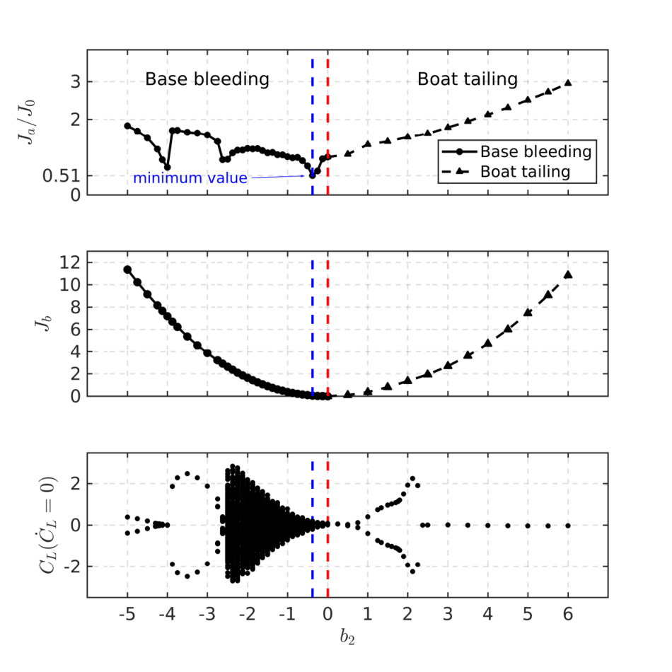
This section describes the behaviour of the fluidic pinball under a symmetric steady actuation. In this configuration, only the two rearward cylinders rotate at equal but opposite rotation speeds, . When is positive, the rearward cylinders accelerate the outer boundary layers and suck near-wake fluid upstream. This forcing delays separation, mimics Coanda forcing and leads to a fluidic boat tailing. When is negative, the cylinders eject fluid in the near wake like in base bleed and oppose the outer boundary-layer velocities. Figure 6 shows the evolution of (top), (middle) and the bifurcation diagram (bottom) as a function of .
We limited our study to . The trends are resolved with a discretization step of and a finer resolution in the ranges and . For each parameter, the cost and actuation power have been computed over 1000 convective time units. The bifurcation diagram has been built by detecting the extrema of the lift coefficient over the last 600 convective time units. The bifurcation diagram reveals five regimes:
- Regime :
-
the lift amplitude decreases to zero and the cost decreases to the first minimum.
- Regime :
-
the extremal lift values increase and decrease to zero again. The cost approaches another local minimum near .
- Regime :
-
a period doubling cascade is observed for decreasing leading to a chaotic regime. At , the cost assumes it global minimum with residual fluctuation of the lift coefficient.
- Regime :
-
the cost and the extremal lift values monotonically increase.
- Regime :
-
the Coanda forcing completely stabilizes a symmetric steady solution. The cost increases with the rotation speed.
Interestingly, the boat tailing discontinuity at does not appear in the graph of the cost function . This continuity, even in the derivative, corresponds to a continuous passage from a periodic symmetrical solution to a stationary solution which is itself symmetrical. As the value of the cost function indicates, this stationary solution is quite far from the unforced symmetric steady solution. The global minimum of is reached near , i.e., for a base bleeding configuration, corresponding to a small actuation power , roughly 0.1% of the .
The characteristics of the best base bleeding solution leading closest to the symmetric steady solution are depicted in figure 7. In figure 7(a), the lift coefficient is displayed for the unforced transient (blue curve) and the forced flow (red curve). The unforced flow terminates in an asymmetric shedding with positive lift values. After the start of forcing, the lift coefficient oscillates vigorously around its vanishing mean value. This forced statistical symmetry is corroborated by the oscillating jet in figures 8(a)-8(h). Base bleed increases the velocity of the rearward jet compared to the unforced flow. This jet instability mitigates the Coanda effect on the bottom and top cylinder, i.e., the jet neither stays long at either side.


The vortex shedding persists similar to the unforced flow. However, the dominant frequency is increase from to . The instantaneous cost function in figure 7(c) shows an unsteady non-periodic behavior, reaching intermittently low levels. The broad spectral peak in figure 7(d) is a characteristic of a chaotic regime. The phase portrait in figure 7(b) corroborates the non-periodic oscillatory behaviour. The mean field in figure 8(j), shows that actuated mean jet is symmetric unlike the mean field of the unforced flow. Moreover, the shear-layer on the upper and lower sides extend further downstream as compared to the unforced state.
This parametric study reveals that base bleeding is the best symmetric steady forcing strategy to bring the flow close to the symmetric steady solution. However, even though the cost is almost halved, the best base bleeding control fails to stabilize the flow.
4.2 General non-symmetric steady actuation—Explorative gradient method
In this section we aim to stabilize the symmetric steady solution by commanding the three cylinders with constant actuation without symmetry constraint. This three-dimensional parameter space is explored with the explorative gradient method presented in section § 3.2. The symmetry along the -axis of the fluidic pinball allows us to reduce our search space and to explore only positive values of . A coarse initial parametric study carried on , and by steps of unity indicates that the global minimum of should be near . Thus, we limit our research to the actuation domain . The limitation of to positive values exploits the mirror symmetry of the configuration. Figure 9 (bottom) depicts the cost function in the actuation domain . Three planes () are computed by interpolating parameters on a coarse grid. The individuals computed with EGM are all shown in the 3D space. The four initial control laws for EGM are the center of the box and shifted points from this center. The shift is of the box size in positive coordinate direction. Thus, the four initial control laws are: , , and . The exploration phase is then performed in . For algorithmic reasons, the explorative points are chosen from 1 million points obtained from a space filling LHS. In the following, denotes the number of evaluations. The optimization processes stops after evaluations. This corresponds to 25 iterations of the exploration/exploitation process. Convergence is already reached around . On one hand, we notice that the exploration phases (LHS in blue) focus on the boundary of the search space. This is consistent with the goal of LHS, as the furthest initial individuals are on the boundary of the box. On the other hand, the exploitation phases (simplex in yellow) stay in the same neighborhood near the initial individuals, crawling along the local gradient to find the minimum.

Figure 10 shows the progression of the best control laws throughout the evaluations after 25 iterations of the exploration/exploitation process. The progression is plotted according to the number of cost function evaluations counted with the dummy index . Figure 10(a) depicts the progression of the best control law after each downhill simplex step. We notice that a plateau is reached after 50 evaluations and there are only small variations afterwards. The final control law after 100 evaluations reads
| (8) |
From visualizations of the control landscape of in figure 9, we can safely infer that (8) describes the global minimum of our search space. Figure 10(b) shows convergence after 70 evaluations. Thereafter, the downhill simplex iterations show negligible improvements. In the whole EGM optimization, the exploration appears to be ineffective as the initial individuals are close to the minimum. An EGM run with different initial individuals ( , , and , corresponding to a of the box size shift) have been tested. After a few iterations, this new run started sliding down towards the same minimum. This can be explained by the fact that the neighborhood around the minimum is smooth enough for a downhill slide of the exploitation individuals.


The control law (8) shows that the front cylinder rotates almost five times faster than the two other cylinders and in opposite directions. The asymmetry in the control law corresponds to the asymmetry in the lift coefficient in figure 11(a), where the mean value is close to -0.7. The flow asymmetry can be visualized in the mean field (figure 12(j)). The vorticity in the vicinity of the cylinder is directly related to the actuation; thus the upward deflection near the front cylinder is explained by its fast rotation, around 1.1 times the incoming velocity. In addition, the tip of the positive vorticity lobe in the jet is slightly deflected downwards. Figure 12(a)-12(h) show that EGM control (8) enables a jet fluctuation around vanishing mean, like the best base bleeding solution. Moreover, the phase portrait and the PSD in figure 11 reveal that the flow is purely harmonic. The main frequency is close to the main frequency of the base bleeding solution. Contrary to the best base bleeding solution, the instantaneous cost function stays at low levels with a mean value around 9. The associated normalized cost is . It is worth noting that, even though the control law is close to the best one found with EGM, its cost, , is much higher. Moreover, the coarse description of the optimal plane , in figure 9 (top), does not show any minimum a priori. This reveals large gradients in the control landscape, near the EGM solution, where a small change in the control amplitude can drastically change the associated cost .


In addition to the less deflected jet, we notice in figure 12 that the vortex shedding differs from the previous solution leading to a more symmetric flow. There are now two vortex shedding of the shear layers, one on the upper side and one on the lower side of the flow. These shear layer dynamics hardly interact in the whole domain. Indeed, we notice that the distance between two consecutive vortices increases significantly only before leaving the computational domain which goes along with a slightly upward deflection of the wake. This results in extended vorticity branches in the mean field (figure 12(j)) but with a lower vorticity level compared to the symmetric steady solution.
As expected, exploring a richer search space improved the stabilization of the flow. However, surprisingly, an asymmetric forcing managed to bring partial symmetry to the flow and reduces the cost function even further compared to the best base bleeding solution. Experimentally, the optimization of the steady fluid pinball actuation also lead to asymmetric forcing Raibaudo et al. 2019. The explorative gradient method managed to converge to the global minimum in less than evaluations. The exploration phases had a lesser impact during the optimization process as we initiated the algorithm close to the global minimum. We can expect the exploration phases to play a major role for more complex search space, comprising several minima.
4.3 Feedback control optimization—Gradient-enriched machine learning control
In this section, we optimize a feedback control law again to stabilize the unforced symmetric steady solution. The feedback is provided by 9 velocity signals in the wake as discussed in § 2.3. Several function optimizers can be used to solve the regression problem of equation 6. However, a comparison between classical MLC (Duriez et al. 2016) and gMLC has been carried out, showing that gradient-enriched MLC not only converges faster than MLC but also towards a better solution. The comparison between MLC and gMLC is detailed in appendix A.
In the case of the fluidic pinball, the three cylinders are our three controllers thus . For the control input space , we choose a grid of nine sensor downstream measuring either or velocity component. The coordinates of the sensors are and . The downstream position of the sensors have been chosen so that good performance of stabilizing feedback control can be expected (Roussopoulos 1993): The position is far enough for pronounced vortex shedding but close enough to avoid phase decorrelation between actuation and sensing. Moreover, sensors at different locations allow to exploit phase differences between the sensors. The six exterior sensors are sensors while sensors are chosen for the ones on the symmetry line , so that the signals vanish when the symmetric steady solution is reached. Experimental realizations are typically based on one or few sensor positions. The large number of 9 positions has the advantage that gMLC may indicate not only the near-optimal control law but also the best sensor location. The information of sensors is summarized in table 2.
| sensor | -coordinate | -coordinate | velocity component |
| 5 | 1.25 | ||
| 6.5 | 1.25 | ||
| 8 | 1.25 | ||
| 5 | 0 | ||
| 6.5 | 0 | ||
| 8 | 0 | ||
| 5 | -1.25 | ||
| 6.5 | -1.25 | ||
| 8 | -1.25 |
We introduce time-delayed sensor signals as inputs to enrich the search space and allow ARMAX-based controllers (Hervé et al. 2012). The delays are a quarter, half and three-quarters of the natural shedding period, yielding following additional lifted sensor signals and allowing to reconstruct the phase of the flow:
For oscillatory signals, the chosen time delay corresponds to the first zero of the auto-correlation function which is a common practice for construction of phase spaces. The four time-delay coordinates is the minimum information to determine the mean value, the amplitude and the phase of each signal at every time step.
Summarizing, the dimension of the sensor vector is and . We do not include time dependent functions in the input space as we aim to stabilize the flow towards the steady solution so an open-loop strategy is not pursued. In appendix B, we detail an open-loop optimization including periodic functions. We show that a symmetric periodic forcing at 3.5 times the natural frequency, manages to stabilize the flow but at the expense of high actuation power. So periodic functions are not included as inputs in order to avoid costly solution. Thus, , and . The control laws are then built from 9 basic operations (, , , , , , , and ), 36 sensors signals and 10 constants. The control laws are restricted to the range to avoid excessive actuation. The basic operations and are protected in order to be defined on in its entirety. The cost function has been computed over 1000 convective time units, so that the post-transient regime is fully established and the transient phase has a lesser weight.
For the implementation of the gMLC algorithm on the fluidic pinball, we start with a Monte Carlo step of individuals, the crossover probability and mutation probability are both set at . Indeed, as the evolution phase is mostly an explorative phase, the mutation probability is increased, from 0.3, in previous studies, to 0.5, to improve the exploration capability. Moreover, even though crossover is an exploitative operator, it is likely to find new minima thanks to recombinations of radically different control laws. That is why, the crossover and mutation probabilities are both set to 0.5. The dimension of the subspace is set to , so it is large enough to explore a rich subspace but not too large to avoid a slowdown in the optimization process. Evidently with a subspace of higher dimension the control law can be more finely tuned. To assure that the subplex step effectively goes down the local minimum, we choose to evaluate individuals during the exploitation phase. Test runs with have been carried out and showed that the learning process was slower. We believe one reason is that each exploration phase changes systematically the subspace, which makes it difficult for the subplex to improve effectively in only a few steps, thus, subplex has almost no benefit in the early phases. Table 3 summarizes all the parameters for gMLC. The secondary optimization problem (equation 7) used to build a matrix representation for the control laws, is solved with LGP. To speed up the computation, we choose to solve the secondary optimization problem with 100 individuals evolving through 10 generations. Finally, our implementation is enhanced by a screening of the individuals to avoid reevaluating individuals that have different mathematical expressions but are numerically equivalent, just as (Cornejo Maceda et al. 2019). This screening is used only in steps where the individuals are generated stochastically, meaning in the Monte Carlo step and in the exploration phases. This improvement is also used in LGP to solve the secondary optimization problem. We choose our stopping criterion to be a total number of evaluations to mimic experimental conditions. In this study, the limit is set to 1000 following prior experience and practical considerations. The authors have observed convergence within this limit for all MLC studies with dozens of configurations. In addition, wind tunnel experiments with 1000 evaluations and 5–20 seconds testing time can easily be performed in one day.
| parameter | description | value |
|---|---|---|
| number of actuators | 3 | |
| number of sensors | 9 sensors 4 delays = 36 | |
| number of periodic functions | 0 | |
| number of Monte Carlo individuals | 100 | |
| subplex size | 10 | |
| crossover probability | 0.5 | |
| mutation probability | 0.5 | |
| number of individuals per phase | 50 | |
| number of constants | 10 | |
| constant range | [-1,1] | |
| operations | , , , , , , , , |
Figure 13 presents the learning process of gMLC for the stabilization of the fluidic pinball. We notice that the first exploration phase, individuals , already improved the best cost compared to the Monte Carlo phase. The following exploitation, individuals , present a steep descent, improving the best solution even further. During this phase, we notice a clear trend for the cost of the new individuals. This trend indicates that the simplex is going down towards a minimum. But this descent is interrupted by the next exploration phase. Individuals , greatly improve the best solution. Particularly, two individuals have a much lower cost that the ones in the simplex, suggesting that a new minima have been found. The next exploitation phase with individuals brings no improvement. The high values of cost in the exploitation steps following the exploration phases is explained by the fact that as we are exploring new minima, shrink steps must be performed to bring the simplex towards the new minima; and the shrink steps replaces all individuals in the simplex except the best one. As we are leaving one minimum for another one, the intermediate values can be arbitrarily high until the simplex reached the neighborhood of the new minimum. The next exploration phase with individuals also give good individuals that have been included in the simplex. After 350 evaluations, the only improvements are performed by exploitation phases. Even if the best cost keeps decreasing slowly, the improvements are small, indicating that we are close to the minimum. Once we reach a plateau, further improvement can only be performed if an exploration phase finds an individual close to a better minimum. That is why after 800 individuals, we performed only exploration phases. The final control law build with gMLC reads
| (9) |


Figure 14 presents the characteristics of the flow controlled by the best control law built with gMLC. This control law is detailed later specially in table 4. In figure 14(a), we can see that even if the resulting lift coefficient is still asymmetric, the mean value (around ) is closer to 0 as compared to the EGM solution. The PSD in figure 14(d) shows a dominant frequency at and one of its higher harmonics. A small peak can be seen for . The nonlinear interaction between the frequencies and gives rise to another small peak at . The phase portrait in figure 14(b) reveals drifts in pronounced oscillations due to the low frequency modulation. The presence of the dominant frequency and its harmonic in the spectrum is consistent with the periodic behavior of the flow. The peak is responsible for the width of a predominant limit-cycle dynamics in the phase portrait.
The evolution of the instantaneous cost function in figure 14(c) shows a plateau after convective time units, reaching an even lower level (around 6), compared to the EGM solution (around 9). The associated cost is better than the EGM solution at .


| cylinder | mean value | main frequency | peak-to-peak amplitude |
|---|---|---|---|
| front (, green) | 0.48 | 2 | 0.12 |
| bottom (, blue) | -0.19 | 2 | 0.03 |
| top (, red) | -0.02 |
Table 4, 5 and figure 16a give more details on the control law built with gMLC. Firstly, we can see that even though the simplex comprises individuals, subplex build the control law by linearly combining 14 control laws. Indeed after a few iterations of simplex, all the individuals are eventually a linear combination of the initial individuals forming simplex. When a new individual is introduced in the basis thanks to the exploration phase, the exploitation phase will combine the remaining individuals with the new one, making the next individual a linear combination of more than 10 individuals. It is important to note that even after the introduction of new individuals with the exploration phase, the subspace to explore changes but the dimension remains. In this case, with , the dimension of the subspace is 9. The repetition of this process builds each time more complex control laws. Thus, in table 4, individuals have been introduced thanks to exploration phases. The control laws with the strongest weights are and , whereas the weight associated with the other control laws are at least one order of magnitude lower. Control law is also the one with the lowest cost . is then mainly based on and corrected by the remaining control laws. This indicates that on the last phase of the learning, it is the minimum in the neighborhood of that has been found.
Moreover, table 4 shows that all three control components , and of the gMLC control law include sensor information. However, figure 16a shows that the actuation command associated with for the two rearward cylinders ( and ) are nearly constant. This is partially due to the low weights associated to the control laws with sensor signals. We can also assume that the sensor signals cancel each other, leading to such low peak-to-peak amplitudes. Table 5 shows the characteristics of the actuation command during the post-transient regime. A spectral analysis shows that the main frequency of the actuation command for the front and bottom cylinder are twice the main frequency of the flow , revealing that the actuation is a function of the flow. Thus, gMLC managed to build a combination between asymmetric steady forcing and feedback control. Finally, like EGM, the best solution found is asymmetric but with lower amplitudes. Consequently, the associated actuation power is lower compared to general steady actuation found with EGM: for the general steady actuation and for the feedback control law found with gMLC.
The controlled flow is depicted over one period in figure 15(a)-15(h). First, we notice that the jet fluctuates around a vanishing mean, as for the EGM actuation. Also, the vortex shedding of the upper and lower shear layers hardly interact. Compared to the EGM solution, the stability of the wake is improved as the two Kelvin-Helmholtz vortices keep their transverse distance to the symmetry line until the very end of the computational domain. This is explained by the re-energization of the shear layers thanks to the vigorous rotation of the front cylinder at twice the main frequency of the controlled flow, like Protas 2004. The mean field, in figure 15(j), is similar to the symmetric steady solution. Indeed, we notice that the vorticity regions extend to the end of the computation domain, like the symmetric steady solution. Also, like for the best general steady actuation, the region near the cylinders is non-symmetrical due to the action. However, contrary to the symmetric steady solution, the mean field of the feedback control has a narrower region between the vorticity regions upstream and a wider region downstream.
As expected, gMLC manages to find a new solution that surpasses the best general steady actuation found with EGM. Surprisingly, gMLC built a non-trivial solution, combining asymmetric steady forcing and feedback control for the front cylinder, controlling the flow with a direct feedback of the phase of the flow, i.e., phasor control (Brunton & Noack 2015). Interestingly, gMLC composed a control law that forces the flow at twice the main frequency. In addition, compared to the best general steady actuation, the actuation power is significantly reduced. Lastly, the learning process of gMLC exploited both the evolution phases and the simplex steps to rapidly build better solutions. Thanks to the evolution phases, new minima have been successfully found and thanks to the simplex steps, the solutions have been improved even more. The progress of the subplex steps show that local gradient information can be exploited in a subspace of an infinite dimension space to minimize a cost function. Building on this success, we believe that gradient-enriched MLC will greatly accelerate the optimization of control laws for MIMO control as compared to the linear genetic programming control.
5 Discussion
This section discusses design aspects of the proposed methodology which are of relevance to this and other configurations. In § 5.1, the role of feedback is assessed. § 5.2 discusses the role of the number of actuators and sensors for the the learning process. In § 5.3, the effect of the dynamics complexity and noise on learning speed is discussed. Finally, robustness for other operating conditions is elaborated in § 5.4.
5.1 The need for feedback
Feedback plays an important role in the gMLC control. Figure 16a shows the corresponding evolution of the actuation commands and instantaneous cost function . The actuation commands lead to constant cylinder rotation with small fluctuation from the sensor signal. The cost function converges to a steady value after some 200 non-dimensional time units. In figure 16b, the actuation commands are replaced by their respective post-transient averaged value of the last 500 time units. Now, the cost function fluctuates periodically between the optimal and the unforced value. The associated averaged cost is and about three times the optimal gMLC value . The important role of feedback is corroborated with another test. The actuation commands of the gMLC control are recorded and applied in an open-loop manner to the flow with a random initial condition. Again, the performance largely fluctuates. Evidently, the small feedback fluctuations play an important role in the stabilization. Intriguingly, similar observations are made by the authors for stabilizing experimental cavity fluctuations and will be described in the dissertation of the first author (Cornejo Maceda 2021).
5.2 Number of sensors and actuators
The control performance is found to increase as the search space is generalized from single parameter steady base bleeding forcing to three parameter steady actuation to feedback with 9 sensors. Generally, increasing the number of actuators and sensors can be expected to enhance the maximum control performance albeit with eventually diminishing returns. On the other hand, the learning time will also increase with the number of actuators and sensors and with the complexity of control laws, e.g., inclusion of time-delay coordinates. Evidently, there is a trade-off between performance gains from increasing the search space and the limitations of the testing time. Like in model identification (Abu-Mostafa et al. 2012, see, e.g.,), one can expect an optimal level of complexity for given testing time. From MLC with dozen’s of configurations (Noack 2019, see, e.g.,), our observation is that the learning time is weakly affected by the number of control law inputs but increases with the number of uncorrelated actuation commands.
The subplex iteration of gMLC is found to significantly accelerate the learning process. Evolutionary methods are known to underperform for convergence of identified minima, i.e., a strength of gradient-based approaches. Gradient-based methods have another advantage of staying in well-performing subspaces. In contrast, genetic operations, like mutation and crossover, tend to bread new individuals leaving these subspaces. These observations are particularly relevant when a symmetry or invariant of the control law is performance critical. The inclusion of known symmetries or invariants in gMLC might be achieved by pre-testing and excluding individuals which strongly depart from these constraints. An example of self-discovery of such symmetries and invariants is reported in Belus et al. 2019 for deep reinforcement learning.
5.3 Complexity of dynamics and noise
The applicability of gMLC to turbulent flows will be addressed in future works starting with Cornejo Maceda 2021. Already MLC has been successfully applied to learning distributed actuation for mixing optimization of a turbulent jet (Zhou et al. 2020). Recent experimental applications of gMLC include mitigation of cavity oscillations, drag reduction of a generic truck model under yaw and lift increase of airfoil under angle of attack at a Reynolds number near one million. Performance and reproducibility of gMLC control are encouraging and outperform other methods, including MLC. Hence, the very optimization principle of iterating between exploration (for discovering new minima) and exploitation (for a fast descent towards the minimum) seems sound. Yet, numerical studies of multi-frequency forcing of the fluidic pinball foreshadow challenges for asymptotic regimes. When the actuation space has many ‘idle’ direction with near constant performance, the gradient-based descent may be trapped in local minima. One cure is a subplex method on ‘active subspaces’ aligned with direction of performance gradients.
Genetic programming is a powerful regression solver which is successfully validated in dozens of experiments, Navier-Stokes simulations, and dynamical systems (Ren et al. 2020; Noack 2019). It can learn complex laws for signals and actuation commands by testing individuals over characteristic times each, i.e., characteristic times in total (Wu et al. 2018; Zhou et al. 2020). Yet, it may not be the most effective choice under several conditions: (1) the total testing time is restricted to much smaller budgets typical for three-dimensional simulations; (2) the control law is smooth or can be expected to depend linearly or affinely to the sensor signals, (3) the flow performance responds immediately to good or bad actuation. Smoothness is well exploited in cluster-based control (Nair et al. 2019). Deep reinforcement learning may learn quickly the optimal actuation in case of fast performance response (Fan et al. 2020; Rabault et al. 2019). A combination of techniques may also benefit a quick learning such as the merging of genetic algorithm and downhill simplex in Maehara & Shimoda 2013. Future work will give more indications about good choices or combinations of machine learning algorithms.
5.4 Robustness of the control
The current study optimizes control for a single Reynolds number. Its robustness will be addressed in future work. We can distill few rules of thumb for robustness from past experience with experiments. First, if the actuation mechanism relies on changing large-scale coherent structures, like synchronizing vortex formation (Parezanović et al. 2016), the control learned for one condition is likely to be robust for a range of conditions. Second, the control law should be learned in a non-dimensional form. For instance, the Strouhal number of an actuation can be expected to be more relevant for different velocities than the value in Hertz unrelated to the velocity change (Gautier et al. 2015). Third, in an ideal scenario, the intended range of operating conditions is already included in the cost function. For instance, a control law may be evaluated at different operating conditions or in a slow transient between them (Asai et al. 2019; Ren et al. 2019). This will, however, dramatically increase the testing time. The learning time saved by smarter algorithms, like gMLC, may be invested in assuring robustness for multiple operating conditions. Tang et al. 2020 provide an inspiring example for deep reinforcement learning.
6 Conclusions
| search space | dimension | method | , | |
| unforced natural | - | - | - |

|
| symmetric steady | 1 | param. study | - |

|
| general steady | 3 | EGM | 77 |

|
| feedback control | gMLC | 800 |

| |
| 250 for | ||||
| feedback control | MLC | 900 |

| |
| periodic forcing | 2 | EGM | 74 |

|
We have stabilized the wake behind a fluidic pinball with three independent cylinder rotations in successively larger search spaces for control laws. Table 17 summarizes the corresponding performances quantified by the average distance between the controlled flow and the steady symmetric solution. First, steady symmetric forcing is employed. A base bleed solution with a cylinder rotation of 28% of the oncoming velocity leads to a flow which is 49% closer to the symmetric solution than the unforced attractor. Other studies also report about a stabilizing effect of base bleed on bluff body wakes (Wood 1964; Bearman 1967). In contrast, Coanda forcing, i.e., two symmetric cylinder rotations which accelerate the outer flow, may completely stabilize the flow. Yet, this new wake has no long vortex bubble and is further away from the symmetric steady solution than the unforced vortex shedding.
Second, a general non-symmetric actuation is optimized with the explorative gradient method. Surprisingly, an asymmetric actuation reduces the average distance between the flow and the steady target solution further to 28% of the unforced value. This asymmetric actuation leads to shear layer vortices which do not interact and thus do not form von Kármán vortices. The mean flow is slightly asymmetric, but largely mimics the elongated steady symmetric solution. The price for the better performance is a larger actuation power (see table 17). Intriguingly, machine learning control also leads to distinctly asymmetric actuation in experiments (Raibaudo et al. 2019) and simulations (Cornejo Maceda et al. 2019) for other cost functions.
Third, a feedback actuation obtained from gradient-enriched machine learning control brings the flow even closer to the steady target solution. The associated actuation power is smaller than the previous optimized steady actuations (see table 17). The actuation is a combination of asymmetric steady forcing and phasor control. The resulting flow looks similar to the optimal asymmetric steady forcing. Figure 18 summarizes the results for the hierarchy of control search spaces.

The feedback control does not seem to have the authority to completely stabilize the symmetric target solution, like for the cylinder wake controlled by a volume force (Gerhard et al. 2003). The wake can be ‘almost’ stabilized for short periods of time, starting from the unforced flow. Then, new coherent structures emerge and lead to residual shear-layer shedding. This lack of complete authority for stabilization may be explained by the complexity of the dynamics. The fluidic pinball has a primary instability associated with von Kármán vortex shedding, a secondary pitchfork instability associated with the centerline jet, and two Kelvin-Helmholtz instabilities of the top and bottom shear layer.
Intriguingly, symmetric high-frequency forcing can bring the flow even closer to the steady target solution but with an actuation power which is roughly two orders of magnitude larger than the previous control laws (see table 17). Protas 2004 and Thiria et al. 2006 also find a stabilizing effect of high-frequency forcing on vortex shedding. The thickening of the shear layers by high-frequency vortices reduces the gradients and thus the instability. To summarize, machine learning control has automatically discovered well known stabilizing mechanisms, like base bleed and phasor control, but added an unexpected asymmetric forcing and combination of this open-loop actuation and phasor feedback for improved performance.
The presented stabilizations are expected to be independent of the employed optimizer as different approaches lead to very similar results. The chosen optimizers balance exploitation (downhill descend of found minima) and exploration (search for better minima). The optimization has been effected in a three-dimensional parameter space for steady forcing and a feedback space with three actuation inputs and nine sensing outputs. Starting point is Latin hypercube sampling as exhaustive exploration of the parameter space and linear genetic programming control as effective regression solver with explorative and exploitive features. The search has been significantly accelerated by intermittently adding gradient-based descends. The resulting explorative gradient method and gradient-enriched machine learning control seem efficient for both exploration and exploitation. Future research shall focus on accelerated learning.
The control performance may be further improved by allowing for more general control laws comprising the history of the sensor signals, like in ARMAX-based control (Hervé et al. 2012). Other generalizations of machine learning control include multiple pre-defined operating conditions, adaptive control for unknown operating conditions, automated learning of the response model from the control law to performance following Fernex et al. 2020 and automated learning of control-oriented modeling based on Li et al. 2020a. The fluidic pinball represents an attractive plant of sufficient dynamic complexity with manageable computational load for these developments.
Acknowledgements
The authors thank Antoine Blanchard, Nan Deng, Luc Pastur and Themis Sapsis for fruitful discussions and enlightening comments. We also thank the anonymous referees for their insightful suggestions. This work is supported by the French National Research Agency (ANR) via FLOwCON project “Contrôle d’écoulements turbulents en boucle fermée par apprentissage automatique” funded by the ANR-17-ASTR-0022, the German National Science Foundation (DFG grants SE 2504/1-1 and SE 2504/3-1), the iCODE Institute, research project of the IDEX Paris-Saclay and by the Hadamard Mathematics LabEx (LMH) through the grant number ANR-11-LABX-0056-LMH in the “Programme des Investissements d’Avenir”.
Declaration of interests
The authors report no conflict of interest.
Appendix A Comparison between MLC and gMLC
In this appendix, we compare the performances of a machine learning control (MLC), based on linear genetic programming control (Li et al. 2018; Zhou et al. 2020), and the proposed gradient-enriched MLC (gMLC) variant for the stabilization of the fluidic pinball. gMLC is described in section § 4.3. MLC differs from gMLC in two respects. First, the evolution is from generation to generation, i.e., groups of individuals. Second, unlike gMLC, no gradient information is employed. The first generation of randomly generated individuals evolves through generations thanks to three genetic operations:
- •
Crossover: a stochastic recombination of two individuals, giving two new individuals exploiting parts of the first two individuals;
- •
Mutation: a stochastic change in one individual, giving one new individual more or less different from the previous one;
- •
Replication: an identical copy of one individual, assuring memory of good individuals throughout the generations.
During the evolution process, the better-performing individuals are selected with larger probability to build new individuals thanks to the genetic operators. The best individuals are selected thanks to a tournament selection method. As in Duriez et al. 2016, we choose a tournament selection of size 7 for 100 individuals. A genetic operation is chosen randomly following given probabilities: the crossover probability , the mutation probability and the replication probability . The probabilities add up to unity . The set of parameters suggested in Duriez et al. 2016 have been chosen for MLC. A parametric study varying , and with a 0.1 step has been carried out on the stabilization of a Landau oscillator by forcing only on one of its components. As MLC is a stochastic process, we perform 100 test runs for each probability combination. This parametric study reveals that this probability combination is one of the best. Among all the probability combinations, this combination is one of those that converges towards better solutions in average, with one of the lowest dispersion of the final solutions over the 100 test runs, showing that this combination is also one of the more robust. This or a very similar probability combination has already been used in Duriez et al. 2016 and dozens of experiments (Noack 2019).
In addition to crossover, mutation and replication, we transfer the best individual of the previous generation to the next one via the elitism operation. This operation assures that the best individual is always in the latest generation so that ‘the winner does not get lost’.
The architecture of the linear programming control laws are the same for MLC and gMLC, including the mathematical operations, number of constants, number of registers, as well as inputs and outputs (see table 3).
The cost function is evaluated over 1000 convective time units, both in MLC and gMLC. The MLC and gMLC algorithms are compared over 1000 evaluations. For MLC, a population of 100 individuals is chosen to evolve over 10 generations. For a fair comparison, MLC and gMLC share the same initial Monte Carlo generation, comprising the first 100 randomly generated individuals. Figure 19 shows the distribution of the costs as a function of the evaluations. We notice that for both algorithms the first exploration phase makes great improvement. In the second generation, the best cost is 0.80 for gMLC and 0.70 for MLC. Note that MLC’s better performance is understandable as 100 individuals have been evaluated for the second generation whereas only 50 individuals have been evaluated for gMLC. After testing 200 individuals, gMLC surpasses MLC thanks to the subplex steps, reaching a cost . For the second evolution phase, both MLC and gMLC perform well reaching low levels of : 0.36 for MLC and 0.26 for gMLC. Then, MLC achieves only small progress after 900 evaluations, the cost improves from 0.36 to 0.33. The series of blue dots at from to represents several instances of the best individual of generation 3, duplicated thanks to elitism. For gMLC, figure 13 shows that evolution phases do not bring any progress after 250 evaluations and further improvement is made thanks to the subplex steps. As described in section § 4.3, the evolution phases help to enrich the simplex subspace. The subplex steps manage to reduce the cost function from 0.26 to 0.20. We notice that after 600 evaluations all new subplex individuals have the same cost. Hence, gMLC surpasses MLC with a smaller number of evaluations and enables improvement/fine-tuning of the control laws in the final phase.

Appendix B Optimal periodic forcing


In this appendix we aim to stabilize the symmetric steady solution thanks to a symmetric periodic forcing. In this case, the two back cylinders oscillate in opposite directions whereas the front cylinder stays still. The control ansatz is the following:
with , the amplitude of the oscillations, and , the frequency, being the two parameter to optimize. The search space is limited to as higher amplitudes and frequencies would be beyond our solver capabilities. This two-dimensional search space is explored with EGM. The contour plot in figure 20 depicts the search space based on and . The contour plot has been produced thanks to simulations for and . The steps are finer for low frequencies and low amplitudes. The individuals have been evaluated over 250 convective time units. We notice that there is only one minimum on the plane, close to . Also, forcing at frequencies close to the natural frequency resonates with the flow and drastically increases the distance to the steady solution for high amplitudes. For , the contour map expectedly displays high values at high frequencies and large amplitudes. The three initial control laws for EGM are the center of the box and increments of 1/5 of the box size in each direction: , , . As expected, the LHS steps (in blue) spread rather evenly in the domain whereas the simplex steps (in yellow) quickly descend into the global minimum.
Figure 21 shows the progression of the best individual throughout the evaluations. The EGM optimization process converges after few tests as , the amplitude and the frequency reach asymptotic values, without any significant improvement afterwards. The parameters of the best symmetric periodic forcing are denoted by the superscript ‘EGM’ and read


The proximity between the initial values and the aimed minimum certainly accelerates the observed convergences. Figure 22 shows the evolution of the lift coefficient, the phase portrait, the power spectral density and the instantaneous cost function for the controlled flow. The lift coefficient presents rather symmetric low amplitude oscillations, see figure 22(a). This goes along with the flow symmetry in figure 23(a)-23(h). The oscillations are explained by the remaining vortex shedding on both, the upper and lower side of the fluidic pinball. Even though the far field is close to the symmetric steady solution, this periodic solution changes radically the near field profile. The jet is completely flattened. We can identify parts of the two vorticity branches close to the cylinders in figure 23(c), 23(d) and 23(e). Moreover, the vorticity around the cylinders is more intense compared to the initial steady solution. This difference is present in the final mean value in figure 22(c) and is responsible for the high actuation power expense, . The phase portrait shows a periodic regime, though deformed by the harmonics. The mean frequency is slightly lower than the forcing frequency and much lower than the natural frequency, showing that it is not just a simple frequency locking, but a nonlinear frequency crosstalk. The non-centered phase portrait indicates that there is still an asymmetry in the flow, that may be a residual effect of the grid’s asymmetry. The mean field in figure 23(j) is similar to the symmetric steady solution, however the jet completely vanishes. In addition, the distance between the upper and lower vorticity branches is wider compared to the symmetric steady solution.


References
- Abu-Mostafa et al. (2012) Abu-Mostafa, Y. S., Magndon-Ismail, M. & Lin, H.-T. 2012 Learning from Data. A Short Course. AMLBook.
- Asai et al. (2019) Asai, S., Yamato, H., Sunada, Y. & Rinoie, K. 2019 Designing machine learning control law of dynamic bubble burst control plate for stall suppression. In 2019 AIAA SciTech Forum. San Diego, CA.
- Barros et al. (2016) Barros, D., Borée, J., Noack, B. R., Spohn, A. & Ruiz, T. 2016 Bluff body drag manipulation using pulsed jets and Coanda effect. J. Fluid Mech. 805, 442–459.
- Bearman (1967) Bearman, P. W. 1967 The effect of base bleed on the flow behind a two-dimensional model with a blunt trailing edge. Aeronautical Quarterly 18 (03), 207–224.
- Belus et al. (2019) Belus, V., Rabault, J., Viquerat, J., Che, Z., Hachem, E. & Reglade, U. 2019 Exploiting locality and translational invariance to design effective deep reinforcement learning control of the 1-dimensional unstable falling liquid film. AIP Advances 9 (12), 125014, arXiv: https://doi.org/10.1063/1.5132378.
- Benard et al. (2016) Benard, N., Pons-Prats, J., Periaux, J., Bugeda, G., Braud, P., Bonnet, J.P. & Moreau, E. 2016 Turbulent separated shear flow control by surface plasma actuator: experimental optimization by genetic algorithm approach. Exp. Fluids 57 (2), 22:1–17.
- Brameier & Banzhaf (2006) Brameier, M. & Banzhaf, W. 2006 Linear Genetic Programming. Springer Science & Business Media.
- Brunton & Noack (2015) Brunton, S. L. & Noack, B. R. 2015 Closed-loop turbulence control: Progress and challenges. Appl. Mech. Rev. 67 (5), 050801:01–48.
- Cattafesta & Shelpak (2011) Cattafesta, L. & Shelpak, M. 2011 Actuators for active flow control. Ann. Rev. Fluid Mech. 43, 247–272.
- Chen et al. (2020) Chen, W., Ji, C., Alam, Md M., Williams, J. & Xu, D. 2020 Numerical simulations of flow past three circular cylinders in equilateral-triangular arrangements. Journal of Fluid Mechanics 891, 1–44.
- Choi et al. (2008) Choi, H., Jeon, W.-P. & Kim, J. 2008 Control of flow over a bluff body. Ann. Rev. Fluid Mech. 40, 113–139.
- Choi et al. (1994) Choi, H., Moin, P. & Kim, J. 1994 Active turbulence control for drag reduction in wall-bounded flows. J. Fluid Mech. 262, 75–110.
- Cornejo Maceda (2021) Cornejo Maceda, G. Y. 2021 Gradient-enriched machine learning control exemplified for shear flows in simulations and experiments. PhD thesis, Université Paris-Saclay.
- Cornejo Maceda et al. (2019) Cornejo Maceda, G. Y., R., Noack B., Lusseyran, F., Deng, N., Pastur, L. & Morzyński, M. 2019 Artificial intelligence control applied to drag reduction of the fluidic pinball. Proc. Appl. Math. Mech. 19 (1), e201900268:1–2.
- Cortelezzi et al. (1994) Cortelezzi, L., Leonard, A. & Doyle, J.C. 1994 An example of active circulation control of the unsteady separated flow past a semi-infinite plate. J. Fluid Mech. 260, 127–154.
- Debien et al. (2016) Debien, A., von Krbek, K. A. F. F., Mazellier, N., Duriez, T., Cordier, L., Noack, B. R., Abel, M. W. & Kourta, A. 2016 Closed-loop separation control over a sharp-edge ramp using genetic programming. Exp. Fluids 57 (3), 40:1–19.
- Deng et al. (2020) Deng, N., Noack, B. R., Morzyński, M. & Pastur, L. R. 2020 Low-order model for successive bifurcations of the fluidic pinball. J. Fluid Mech. 884, A37.
- Dowling & Morgans (2005) Dowling, A. P. & Morgans, A. S. 2005 Feedback control of combustion oscillations. Annual Review of Fluid Mechanics 37 (151–182).
- Dracopoulos (1997) Dracopoulos, D. C. 1997 Evolutionary Learning Algorithms for Neural Adaptive Control. London, etc.: Springer-Verlag.
- Duriez et al. (2016) Duriez, T., Brunton, S. L. & Noack, B. R. 2016 Machine Learning Control — Taming Nonlinear Dynamics and Turbulence, Fluid Mech. its Appl., vol. 116. Springer-Verlag.
- Fan et al. (2020) Fan, S. L., Yang, L., Wang, Z. C., Triantafyllou, M. S. & Karniadakis, G. M. 2020 Reinforcement learning for bluff body active flow control in experiments and simulations. Proc. Natl. Acad. Sci. USA 117 (42), 26091–26098.
- Fernex et al. (2020) Fernex, D., Semann, R., Albers, M., Meysonnat, P. S, Schröder, W. & Noack, B. R. 2020 Self-similar drag reduction formula from sparse data—Optimization of turbulent skin-friction via spanwise travelling surface waves. Phys. Rev. Fluids 5 (7), 073901:1–18.
- Flügel (1930) Flügel, G. 1930 Ergebnisse aus dem Strömungsinstitut der Technischen Hochschule Danzig. In Jahrbuch der Schiffbautechnischen Gesellschaft, pp. 87–113. Springer.
- Fukagata & Nobuhide (2003) Fukagata, K. & Nobuhide, K. 2003 Drag reduction in turbulent pipe flow with feedback control applied partially to wall. Int. J. Heat Fluid Flow 24, 480–490.
- Gautier et al. (2015) Gautier, N., Aider, J.-L., Duriez, T., Noack, B. R., Segond, M. & Abel, M. W. 2015 Closed-loop separation control using machine learning. J. Fluid Mech. 770, 424–441.
- Gelbert et al. (2012) Gelbert, G., Moeck, J. P., Paschereit, C. O. & King, R. 2012 Advanced algorithms for gradient estimation in one-and two-parameter extremum seeking controllers. J. Process Control 22 (4), 700–709.
- Gerhard et al. (2003) Gerhard, J., Pastoor, M., King, R., Noack, B. R., Dillmann, A., Morzyński, M. & Tadmor, G. 2003 Model-based control of vortex shedding using low-dimensional Galerkin models. In 33rd AIAA Fluids Conference and Exhibit. Orlando, Florida, USA, June 23–26, 2003, paper 2003-4262.
- Geropp (1995) Geropp, D. 1995 Process and device for reducing the drag in the rear region of a vehicle, for example, a road or rail vehicle or the like. United States Patent US 5407245 A.
- Geropp & Odenthal (2000) Geropp, D. & Odenthal, H.-J. 2000 Drag reduction of motor vehicles by active flow control using the Coanda effect. Exp. Fluids 28 (1), 74–85.
- Glezer et al. (2005) Glezer, A., Amitay, M. & Honohan, A.M. 2005 Aspects of low- and high-frequency actuation for aerodynamic flow control. AIAA Journal 43 (7), 1501–1511.
- Hervé et al. (2012) Hervé, A., Sipp, D., Schmid, P. J. & Samuelides, M. 2012 A physics-based approach to flow control using system identification. J. Fluid Mech. 702, 26–58.
- Ishar et al. (2019) Ishar, R., Kaiser, E., Morzynski, M., Albers, M., Meysonnat, P., Schröder, W. & Noack, B. R. 2019 Metric for attractor overlap. J. Fluid Mech. 874, 720–752.
- Jordan & Colonius (2013) Jordan, P. & Colonius, T. 2013 Wave packets and turbulent jet noise. Ann. Rev. Fluid Mech. 45, 173–195.
- Koumoutsakos et al. (2001) Koumoutsakos, P., Freund, J. & Parekh, D. 2001 Evolution strategies for automatic optimization of jet mixing. AIAA J. 39 (5), 967–969.
- Li et al. (2020a) Li, H., Fernex, D., Tan, J., Morzyński, M. & Noack, B. R. 2020a Cluster-based network model of an incompressible mixing layer. J. Fluid Mech. submitted, http://arxiv.org/abs/2001.02911.
- Li et al. (2019) Li, R., Borée, J., Noack, B. R., Cordier, L. & Harambat, F. 2019 Drag reduction mechanisms of a car model at moderate yaw by bi-frequency forcing. Phys. Rev. Fluids 4 (3), 034604.
- Li et al. (2018) Li, R., Noack, B. R., Cordier, L., Borée, J., Kaiser, E. & Harambat, F. 2018 Linear genetic programming control for strongly nonlinear dynamics with frequency crosstalk. Archives of Mechanics 70 (6), 505–534.
- Li et al. (2020b) Li, Y., Cui, W., Jia, Q., Li, Q., Yang, Z., Morzyński, M. & Noack, B. R. 2020b Explorative gradient method for active drag reduction of the fluidic pinball and slanted ahmed body. J. Fluid Mech. (in revision, see arXiv).
- Luchtenburg et al. (2009) Luchtenburg, D. M., Günter, B., Noack, B. R., King, R. & Tadmor, G. 2009 A generalized mean-field model of the natural and actuated flows around a high-lift configuration. J. Fluid Mech. 623, 283–316.
- Maehara & Shimoda (2013) Maehara, N. & Shimoda, Y. 2013 Application of the genetic algorithm and downhill simplex methods (nelder–mead methods) in the search for the optimum chiller configuration. Applied Thermal Engineering 61 (2), 433 – 442.
- McKay et al. (1979) McKay, M. D., Beckman, R. J. & Conover, W. J. 1979 A comparison of three methods for selecting values of input variables in the analysis of output from a computer code. Technometrics 21 (2), 239–245.
- Nair et al. (2019) Nair, A., Yeh, C.-A., Kaiser, E., Noack, B. R., Brunton, S. L. & Tiara, K. 2019 Cluster-based feedback control of turbulent post-stall separated flows. J. Fluid Mech. 875, 345–375.
- Nelder & Mead (1965) Nelder, J. A. & Mead, R 1965 A simplex method for function minimization. Computer Journal 7 (4), 308–313.
- Noack (2019) Noack, B. R. 2019 Closed-loop turbulence control—From human to machine learning (and retour). In Proceedings of the 4th Symposium on Fluid Structure-Sound Interactions and Control (FSSIC), Tokyo, Japan (ed. Y. Zhou, M. Kimura, G. Peng, A. D. Lucey & L. Hung), pp. 23–32. Springer.
- Noack et al. (2003) Noack, B. R., Afanasiev, K., Morzyński, M., Tadmor, G. & Thiele, F. 2003 A hierarchy of low-dimensional models for the transient and post-transient cylinder wake. J. Fluid Mech. 497, 335–363.
- Noack et al. (2016) Noack, B. R., Stankiewicz, W., Morzyński, M. & Schmid, P. J. 2016 Recursive dynamic mode decomposition of transient and post-transient wake flows. J. Fluid Mech. 809, 843–872.
- Parezanović et al. (2016) Parezanović, V., Cordier, L., Spohn, A., Duriez, T., Noack, B. R., Bonnet, J.-P., Segond, M., Abel, M. & Brunton, S. L. 2016 Frequency selection by feedback control in a turbulent shear flow. J. Fluid Mech. 797, 247–283.
- Pastoor et al. (2008) Pastoor, M., Henning, L., Noack, B. R., King, R. & Tadmor, G. 2008 Feedback shear layer control for bluff body drag reduction. J. Fluid Mech. 608, 161–196.
- Pfeiffer & King (2012) Pfeiffer, J. & King, R. 2012 Multivariable closed-loop flow control of drag and yaw moment for a 3d bluff body. In 6th AIAA Flow Control Conference, pp. 1–14. Atlanta, Georgia, USA.
- Protas (2004) Protas, B. 2004 Linear feedback stabilization of laminar vortex shedding based on a point vortex model. Phys. Fluids 16 (12), 4473–4488.
- Rabault et al. (2019) Rabault, J., Kuchta, M., Jensen, A., Réglade, U. & Cerardi, N. 2019 Artificial neural networks trained through deep reinforcement learning discover control strategies for active flow control. J. Fluid Mech. 865, 281–302.
- Raibaudo et al. (2019) Raibaudo, C., Zhong, P., Noack, B. R. & Martinuzzi, R. J. 2019 Machine learning strategies applied to the control of a fluidic pinball. Phys. Fluids 32, 015108.
- Ren et al. (2020) Ren, F., Hu, H.-B. & Tang, H. 2020 Active flow control using machine learning: A brief review. J. Hydrodyn. 32 (2), 247–253.
- Ren et al. (2019) Ren, F., Wang, C. & Tang, H. 2019 Active control of vortex-induced vibration of a circular cylinder using machine learning. Physics of Fluids 31 (9), 093601, arXiv: https://doi.org/10.1063/1.5115258.
- Roussopoulos (1993) Roussopoulos, K. 1993 Feedback control of vortex shedding at low Reynolds numbers. J. Fluid Mech. 248, 267–296.
- Rowan (1990) Rowan, T. 1990 The subplex method for unconstrained optimization. PhD thesis, PhD thesis, Department of Computer Sciences, University of Texas.
- Rowley & Williams (2006) Rowley, C. W. & Williams, D. R. 2006 Dynamics and control of high-Reynolds number flows over open cavities. Ann. Rev. Fluid Mech. 38, 251–276.
- Seifert (2012) Seifert, J. 2012 A review of the Magnus effect in aeronautics. Prog. Aerosp. Sci. 55, 17–45.
- Semaan et al. (2016) Semaan, R., Kumar, P., Burnazzi, M., Tissot, G., Cordier, L. & Noack, B. R. 2016 Reduced-order modeling of the flow around a high-lift configuration with unsteady Coanda blowing. J. Fluid Mech. 800, 71–110.
- Tang et al. (2020) Tang, H., Rabault, J., Kuhnle, A., Wang, Y. & Wang, T. 2020 Robust active flow control over a range of reynolds numbers using an artificial neural network trained through deep reinforcement learning. Physics of Fluids 32 (5), 053605, arXiv: https://doi.org/10.1063/5.0006492.
- Thiria et al. (2006) Thiria, B., Goujon-Durand, S. & Wesfreid, J. E. 2006 The wake of a cylinder performing rotary oscillations. J. Fluid Mech. 560, 123–147.
- Wood (1964) Wood, C. J. 1964 The effect of base bleed on a periodic wake. J. R. Soc. Interface 68 (643), 477–482.
- Wu et al. (2018) Wu, Z., Fan, D., Zhou, Y., Li, R. & Noack, B. R. 2018 Jet mixing enhancement using machine learning control. Exp. Fluids 59, 131:1–17.
- Zhou et al. (2020) Zhou, Y., D., Fan, Zhang, B., , Li, R. & Noack, B. R. 2020 Artificial intelligence control of a turbulent jet. J. Fluid Mech. 897, 1–46.