Fast Convergence Algorithm for Analog Federated LearningThanks: 

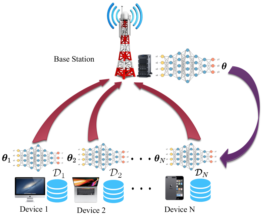
We consider a federated edge learning system consisting of $N$ single-antenna edge devices indexed by set $\mathcal{N}=\{1,2,\ldots,N\}$ and a computing enabled edge server equipped with a single antenna, as illustrated in Fig. 1. Each device $n$ is associated with its own local dataset $\mathcal{D}_{n}$, and all edge devices collaboratively learn a shared global model by communicating with the edge server.

In federated learning systems, the goal is to learn a shared global model by minimizing the sum of the devices’ local loss function. Therefore, the problem can be formulated as the following consensus federated optimization problem:

where $\bm{\theta}\in\mathbb{R}^{d}$ is the global model with dimension $d$. For each device $n$, $\bm{\theta}_{n}\in\mathbb{R}^{d}$ is the local model and $f_{n}$ is the local loss function defined by the learning task and the local dataset $\mathcal{D}_{n}$.

To solve problem (II-A), we adopt the Fedsplit algorithm proposed in [13], which is based on the operator splitting procedures. As depicted in Fig. 1, at each $t$-th communication round, the edge server broadcasts the current global model $\bm{\theta}^{t}$ to all edge devices via the downlink channel through the digital communication. Hence, the power constraint of the edge server is not as strict as the edge devices, and the downlink communication is assumed to be error-free [12, 11, 14]. Consequently, each device receives the current shared global model $\bm{\theta}^{t}$ without distortion. Based on the received current global model $\bm{\theta}^{t}$ and the local dataset $\mathcal{D}_{n}$, device $n$ updates the local model $\bm{\theta}^{t+1}_{n}$ with two steps as follows.

1. 1.

   Local prox step:

   $\displaystyle\bm{\theta}^{t+1/2}_{n}\triangleq\operatorname{prox}_{s,n}(2\bm{\theta}^{t}-\bm{\theta}^{t}_{n}),$

   (3)

2. 2.

   Local centering step:

   $\displaystyle\bm{\theta}^{t+1}_{n}\triangleq\bm{\theta}^{t}_{n}+2(\bm{\theta}^{t+1/2}_{n}-\bm{\theta}^{t}),$

   (4)

where the proximal operator $\operatorname{prox}_{s,n}$ is defined by

for some step size $s>0$.

After updating local models, the edge devices transmit a function of the local model over a wireless fading multiple access channel (MAC) to the edge server. By exploiting over-the-air computation (AirComp), the edge server aggregates all devices local models in one channel use [9], which significantly reduces communication latency. Based on the received signals, the edge server is able to obtain an estimate $\bm{\hat{\theta}}^{t+1}$ of the average global model

The whole procedure will continue until meeting a convergence condition.

Consider the case when each local loss function $f_{n}$ is both $\ell_{n}$-strongly convex and $L_{n}$-smooth. We define the condition number of the problem $\kappa=\frac{L^{*}}{\ell_{*}}$ where $\ell_{*}=\min_{n\in N}\ell_{n}$ is the smallest strong convexity constant and $L^{*}=\max_{n\in N}L_{n}$ is the largest Lipschitz constant. Then we have the following results, which has been proved in [13, Section 5].

Remark 1: To address problem (II-A), a number of different methods have been proposed, e.g., FedAvg [15] and FedProx [16]. However, these methods guarantee convergence to fixed points, but not necessarily optimal solutions, even in strongly convex settings [13, 17]. Furthermore, the iteration complexities of these algorithms will increase significantly when the problem becomes ill-conditioning. In constrast, the FedSplit algorithm enjoys global optimality and linear convergence rate when the local loss functions are strongly convex. In addition, the FedSplit algorithm is robust to the condition number of the problem. Nevertheless, the authors in [13] consider both uplink and downlink channels are error-free, which is indeed unpractical due to limited communication resources in wireless federated learning. Hence, in this paper, we study a more practical implementation of the FedSplit algorithm over a noisy fading MAC.

In this paper, all edge devices communicate with the edge server over the shared wireless MAC channel via AirComp. In this case, coding is unnecessary for an AirComp system to achieve the optimal tradeoff between computation rate and accuracy [18]. Hence, this paper adopts an uncoded nonorthogonal multiple access (NOMA) protocol. Under this setup, we assume a block flat-fading channel, where the channel coefficient remains same during one communication block. Each block is assumed to contain $d$ time slots, so that a $d$-dimensional local model is allowed to transmit within one block. Due to limited memory and computational capacity, the models on edge devices are usually tiny, and may consist of only thousands of parameters [19]. Since typical coherence blocks also have the same order of magnitude [20], it is possible to transmit a model vector in one transmission block. For large model dimensions, we can transmit the models during multiple consecutive coherence blocks, which will slightly affect the analysis. Hence, this paper mainly focuses on the former case.

In this paper, the number of blocks is assumed to be equal to the number of iterations, so that all devices upload their local models in the $t$-th iteration corresponding to the $t$-th block. Then, the received signal at the edge server is given by

where $h_{n}^{t}\in\mathbb{C}$ is the channel coefficient for device $n$ in the $t$-th block; $\bm{w}_{n}^{t}\in\mathbb{C}^{d}$ denotes the additive noise i.i.d according to $\mathcal{CN}(0,\sigma^{2}_{w}\mathbf{I})$; and transmitted signal $\bm{x}_{n}^{t}$ encodes the information about the local model $\bm{\theta}^{t}_{n}$. In addition, the transmit power constraint of each device is given by

with $P_{0}$ as the maximum transmit power.

Based on the received signal $\bm{y}^{t}$, the edge server needs to recover the average global model (6) via AirComp. However, due to the distortion and noise caused by wireless channels, the edge server can only use the perturbed information about local models received from the devices to update the global model. In addition, these factors will greatly affect the convergence of the FedSplit algorithm. Hence, this paper aims to develop a reliable transceiver strategy based on the FedSplit algorithm in wireless communication systems. The strategy includes precoding local models at edge devices and recovering the average global model at edge server. In the following, we will propose the AirComp based Fedsplit Algorithm, and then provide convergence analysis in section III.

In this paper, we assume that perfect CSI are available on all devices and the edge sever, which can be achieved by pilot based methods. For implementation of AirComp, each device is required to perform magnitude alignment to reduce the received signal to the desired average global model (6). By exploiting the knowledge of CSI, each device is able to implement channel inversion by multiplying the local model by its inverse channel coefficient. Specifically, in the $t$-th iteration, device $n$ encodes its local model $\bm{\theta}^{t}_{n}$ into the transmitted signal $\bm{x}^{t}_{n}$ via

where $\sqrt{\alpha^{t}}$ is a uniform scaling factor in the $t$-th iteration. The uniform scaling factor $\sqrt{\alpha^{t}}$ satisfies the power constraint (8), likely,

which implies $\sqrt{\alpha^{t}}\triangleq\min_{n\in\mathcal{N}}\frac{|h_{n}^{t}|\sqrt{P_{0}}}{\|\bm{\theta}_{n}^{t}\|_{2}}$. However, it is obvious to note that weak channels (i.e., $|h^{n}_{t}|\approx 0$) results in the small scaling factor $\sqrt{\alpha^{t}}$. Consequently, the received signals will be weakened and the interference caused by channel noise will significantly increase. This suggests that uniform channel inversion may not be always desirable and the optimal power-control policy for AirComp should be adapted to multiuser CSI. Therefore, we propose a binary scheme of device selection based on multiuser CSI. In particular, a threshold $\gamma$ is set for device selection, and edge devices observing fading coefficients of a smaller magnitude than $\gamma$ do not transmit in the corresponding communication round. Under this scheme, the transmitted signals (9) become

where the indicator of device selection $\beta^{t}_{n}$ is defined by

with some threshold $\gamma\geq 0$. Hence, the scaling factor becomes $\sqrt{\alpha^{t}}=\min_{n\in\mathcal{B}}\frac{|h_{n}^{t}|\sqrt{P_{0}}}{\|\bm{\theta}_{n}^{t}\|_{2}}$.

To simplify, we denote $\mathcal{B}^{t}\subseteq\mathcal{N}$ as the set of participating devices indices subject to $\beta^{t}_{n}=1$. Since the edge server is assumed to know all CSI, it also knows $\mathcal{B}^{t}$ by (II-D). Hence, the average global model (6) can be recovered by the edge server as follows,

where $\bar{\bm{\theta}}^{t}\triangleq\frac{1}{|\mathcal{B}^{t}|}\sum_{n\in\mathcal{B}^{t}}\bm{\theta}_{n}^{t}$ and $\bm{\tilde{w}}^{t}$ is the equivalent additive noise according to $\mathcal{CN}(0,\frac{\sigma^{2}_{w}}{\alpha^{t}|\mathcal{B}^{t}|^{2}}\mathbf{I})$. The resulting algorithm with $T$ communication rounds is summarized in Algorithm 1.

Assumptions 1 and 2 are commonly used in analyzing FL algorithm for many learning-based tasks, i.e., linear regression and logistic regression. Assumption 3 can be implemented by the following distributed mechanism. At each communication round $t$, we choose the top $B$ devices among the participating device set $\mathcal{B}^{t}$ in term of their CSI, i.e., $|h^{t}_{n}|$, to transmit their signals. If the event of $|\mathcal{B}_{t}|<B$ happens, the devices need wait to the next communication round. Actually, the probability of the event is very small especially when $N$ is large and $\gamma$ is small. This mechanism guarantees $|\mathcal{B}_{t}|=B$ at each iteration. Notice that Assumption 3 is only used for convergence analysis. In fact, when AirComp based Fedsplit is implemented without such a mechanism, i.e., $|\mathcal{B}_{t}|$ is random, it will achieve similar convergence characteristics. The authors in [21] have made similar assumptions.

Based on the above assumptions, we present the convergence of the sequence $\{\hat{\bm{\theta}}^{t}\}$ as follows.

Remark 2: Theorem 2 shows that it is able to achieve the convergence rate of the FedSplit algorithm, i.e., linear convergence. Note that the iteration complexity remains $T(\epsilon,\kappa)=O\left(\sqrt{\kappa}\log(1/\epsilon)\right)$ as claimed in Theorem 1, whereas the GD based algorithms for the wireless FL problem proposed in [12, 11] are linearly dependent of the condition number, i.e., $T(\epsilon,\kappa)=O\left(\kappa\log(1/\epsilon)\right)$. Hence, we can conclude that our algorithm is more robust to the ill-conditioned problems. What’s more, Theorem 2 establishes a finite bound of the estimation error for strongly convex and smooth local loss functions over fading MAC. The error bound is characterized by two terms, the initial distance due to the error in the initial estimate and the additive noise caused by the channel noise. In the case of error-free channels, our algorithm can be reduced to the FedSplit algorithm, and thus achieves the same performance. In addition, the design of the threshold $\gamma$ will greatly affect the additive noise term, which will be discussed in our future work.

In this case, we generate random matrices $X_{n}\in\mathbb{R}^{m_{n}\times d}$ with $(X_{n})_{uv}\overset{\mathrm{i.i.d}}{\sim}\mathcal{N}(0,1)$, for all $n\in\mathcal{N}$, $u\in[m_{n}]$ and $v\in[d]$. The simulation parameters are set as

thus satisfying that all $X_{n}$ are full rank due to $m_{n}\gg d$ for all device $n$, which is called as well-conditioned setting.

Except GBMA, we also compare AirComp based FedSplit Algorithm with following algorithms: (i) original FedSplit algorithm; (ii) FedSGD algorithm, $e=1$, which is the original version of GBMA without channel distortion, where $e$ is the number of local gradient steps. After defining these parameters, we run simulations according to (20) and (21) with Rayleigh channel gain and additive noise defined before. The simulation results are shown in Fig. 2.

As illustrated in Fig. 2, although both GBMA and AirComp based FedSplit achieve a linear convergence rate, GBMA has a larger error gap, i.e., $10^{-2}$ while AirComp based FedSplit can converge to a more accurate solution, i.e., $10^{-4}$. Besides, AirComp based FedSplit and original FedSplit have the same convergence rate at the beginning. However, due to fading channels and additive noise, there is still a boundary between the solution obtained by the former and the latter, which corresponds to our theoretical analysis.

To verify the effectiveness of our algorithm under ill-conditioned setting, we consider the linear regression problem with different ill-conditioned setting in term of the condition number $\kappa$. The detail of generating the design matrix $X_{n}$ under different condition numbers can be found in [13, Section 4.3]. Similarly, we use i.i.d Rayleigh channel gains and additive Gaussian noise for each device to simulate real situation. The other parameters are set as follows,

By running experiments for $\kappa\in\mathcal{K}=\{10^{2},10^{3},10^{4}\}$, we are able to plot the log gaps of different $\kappa$ from the two algorithms versus communication round $t$. Fig. 3 shows that all the algorithms can achieve linear convergence rate. Besides, when the condition number $\kappa$ increases, the convergence will slow down. In particular, the convergence rate of AirComp based Fedsplit is less sensitive than GBMA in ill-condition cases, which means AirComp based Fedsplit is more robust to the condition number than GBMA. In other words, for ill-conditioned problems and wireless environment, AirComp based Fedsplit is faster and able to achieve higher accuracy compared with GBMA.

References

- [1] T. Li, A. K. Sahu, A. Talwalkar, and V. Smith, “Federated learning: Challenges, methods, and future directions,” IEEE Signal Processing Magazine, vol. 37, no. 3, pp. 50–60, 2020.
- [2] S. Wang, T. Tuor, T. Salonidis, K. K. Leung, C. Makaya, T. He, and K. Chan, “Adaptive federated learning in resource constrained edge computing systems,” IEEE Journal on Selected Areas in Communications, vol. 37, no. 6, pp. 1205–1221, 2019.
- [3] Q. Yang, Y. Liu, T. Chen, and Y. Tong, “Federated machine learning: Concept and applications,” ACM Trans. Intell. Syst. Technol., vol. 10, no. 2, p. 19, Jan. 2019. [Online]. Available: https://doi.org/10.1145/3298981
- [4] W. Y. B. Lim, N. C. Luong, D. T. Hoang, Y. Jiao, Y. C. Liang, Q. Yang, D. Niyato, and C. Miao, “Federated learning in mobile edge networks: A comprehensive survey,” IEEE Communications Surveys Tutorials, vol. 22, no. 3, pp. 2031–2063, 2020.
- [5] M. Chen, Z. Yang, W. Saad, C. Yin, H. V. Poor, and S. Cui, “A joint learning and communications framework for federated learning over wireless networks,” IEEE Transactions on Wireless Communications, pp. 1–1, 2020.
- [6] D. Wen, M. Bennis, and K. Huang, “Joint parameter-and-bandwidth allocation for improving the efficiency of partitioned edge learning,” IEEE Transactions on Wireless Communications, pp. 1–1, 2020.
- [7] H. H. Yang, Z. Liu, T. Q. S. Quek, and H. V. Poor, “Scheduling policies for federated learning in wireless networks,” IEEE Transactions on Communications, vol. 68, no. 1, pp. 317–333, 2020.
- [8] J. Ren, Y. He, D. Wen, G. Yu, K. Huang, and D. Guo, “Scheduling for cellular federated edge learning with importance and channel awareness,” IEEE Transactions on Wireless Communications, pp. 1–1, 2020.
- [9] K. Yang, T. Jiang, Y. Shi, and Z. Ding, “Federated learning via over-the-air computation,” IEEE Transactions on Wireless Communications, vol. 19, no. 3, pp. 2022–2035, 2020.
- [10] G. Zhu, Y. Wang, and K. Huang, “Broadband analog aggregation for low-latency federated edge learning,” IEEE Transactions on Wireless Communications, vol. 19, no. 1, pp. 491–506, 2020.
- [11] M. Mohammadi Amiri and D. Gündüz, “Machine learning at the wireless edge: Distributed stochastic gradient descent over-the-air,” IEEE Transactions on Signal Processing, vol. 68, pp. 2155–2169, 2020.
- [12] T. Sery and K. Cohen, “On analog gradient descent learning over multiple access fading channels,” IEEE Transactions on Signal Processing, vol. 68, pp. 2897–2911, 2020.
- [13] R. Pathak and M. J. Wainwright, “FedSplit: An algorithmic framework for fast federated optimization,” arXiv e-prints, p. arXiv:2005.05238, May 2020.
- [14] M. M. Amiri and D. Gündüz, “Federated learning over wireless fading channels,” IEEE Transactions on Wireless Communications, vol. 19, no. 5, pp. 3546–3557, 2020.
- [15] H. Brendan McMahan, E. Moore, D. Ramage, S. Hampson, and B. Agüera y Arcas, “Communication-Efficient Learning of Deep Networks from Decentralized Data,” arXiv e-prints, p. arXiv:1602.05629, Feb. 2016.
- [16] T. Li, A. K. Sahu, M. Zaheer, M. Sanjabi, A. Talwalkar, and V. Smith, “Federated Optimization in Heterogeneous Networks,” arXiv e-prints, p. arXiv:1812.06127, Dec. 2018.
- [17] G. Malinovsky, D. Kovalev, E. Gasanov, L. Condat, and P. Richtárik, “From Local SGD to Local Fixed-Point Methods for Federated Learning,” arXiv e-prints, accepted by ICML 2020, p. arXiv:2004.01442, Apr. 2020.
- [18] B. Nazer and M. Gastpar, “Computation over multiple-access channels,” IEEE Transactions on Information Theory, vol. 53, no. 10, pp. 3498–3516, 2007.
- [19] S. Ravi, “Efficient on-device models using neural projections,” in International Conference on Machine Learning, 2019, pp. 5370–5379.
- [20] S. Wang, K. Guan, D. He, G. Li, X. Lin, B. Ai, and Z. Zhong, “Doppler shift and coherence time of 5g vehicular channels at 3.5 ghz,” in 2018 IEEE International Symposium on Antennas and Propagation USNC/URSI National Radio Science Meeting, 2018, pp. 2005–2006.
- [21] T. Sery, N. Shlezinger, K. Cohen, and Y. C. Eldar, “Over-the-Air Federated Learning from Heterogeneous Data,” arXiv e-prints, p. arXiv:2009.12787, Sep. 2020.
- [22] X. Li, K. Huang, W. Yang, S. Wang, and Z. Zhang, “On the convergence of fedavg on non-iid data,” arXiv preprint arXiv:1907.02189, 2019.