A quantum optics approach to photoinduced electron transfer in cavities

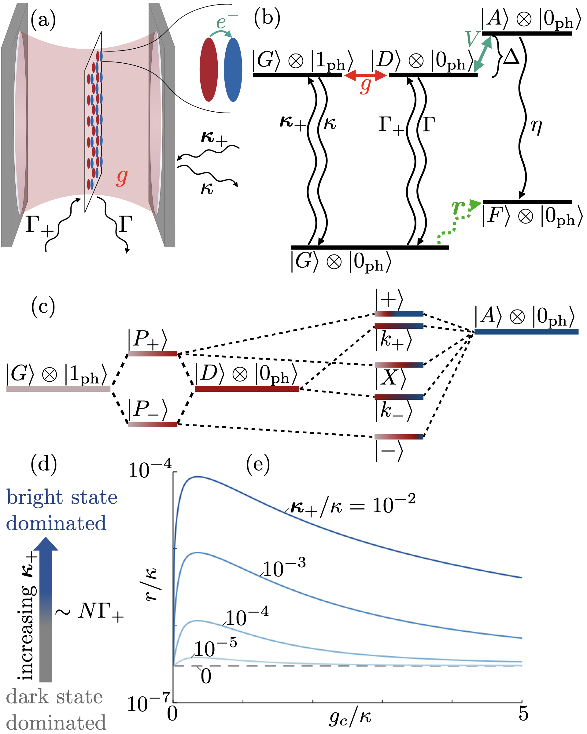
We consider a model of $N$ donor-acceptor pairs homogeneously coupled to a single-mode cavity as schematically depicted in Fig. 1(a). Each donor-acceptor pair is described by a 4-level system with a ground state $\ket{G}$, an excited donor state $\ket{D}$, an excited acceptor state $\ket{A}$, and a final state $\ket{F}$; the cavity is described by a photon mode with annihilation operator $\hat{a}$. We are interested in the transfer dynamics from $\ket{G}$ to $\ket{F}$. The cavity is resonantly coupled to the $\ket{G}\leftrightarrow\ket{D}$ transition with single molecule coupling strength $g$. We further include the following dissipative processes: incoherent cavity pumping at rate $\kappa_{+}$, leading to the creation of a cavity photon, cavity decay at rate $\kappa$, leading to loss of photons from the cavity, pumping of the individual pairs from their ground state $\ket{G}$ to donor state $\ket{D}$ at rate $\Gamma_{+}$, the inverse decay process $\Gamma$, and an artificially introduced non-radiative relaxation from the acceptor state $\ket{A}$ to the final state $\ket{F}$ at rate $\eta$. The corresponding level scheme including the cavity states $\ket{0_{\rm ph}}$ and $\ket{1_{\rm ph}}$ with zero and one photon, respectively, is shown in Fig 1(b).

We set $\hbar=1$ and work in a rotating frame ¹¹ 1 Precisely, the rotating frame transformation is achieved by applying the unitary operator $\hat{U}=\exp[{\rm i}\omega_{DG}t\hat{N}_{e}]$, where the Hamiltonian and the states transform according to $\hat{H}^{\prime}=\hat{U}\hat{H}\hat{U}^{\dagger}+{\rm i}(\partial_{t}\hat{U})\hat{U}^{\dagger}$ and $\ket{\psi'}=\hat{U}\ket{\psi}$, respectively. where we include the bare excited state energies derived from the operator $\hat{N}_{e}\omega_{DG}+\hat{N}_{F}\omega_{FG}=\hat{N}_{e}(E_{D}-E_{G})+\hat{N}_{F}(E_{F}-E_{G})$ in the definition of the states. Here, the operator $\hat{N}_{e}=\hat{N}_{D}+\hat{N}_{A}+\hat{a}^{\dagger}\hat{a}$ gives the excitation number, with the population number operators $\hat{N}_{\psi}=\sum_{n}\ket{\psi}\bra{\psi}_{n}$, $\psi\in\{G,D,A,F\}$, and the subscript $n$ labeling the $n$th pair. We also make the rotating wave approximation, and neglect all counter-rotating terms, which is valid for $g_{c}\equiv\sqrt{N}g\ll\omega_{DG}$ Mandal, Krauss, and Huo 2020. Under these considerations, all coherent dynamics is described by the Hamiltonian

The first line on the right hand side of Eq. (2) describes the contributions due to the energy difference $\Delta=E_{A}-E_{D}$ between the states $\ket{A}$ and $\ket{D}$, and the coherent coupling of the two states with strength $V$ associated with the tunneling of an electron from the donor to the acceptor. The second line describes Tavis-Cummings like coupling between the transition $\ket{G}\leftrightarrow\ket{D}$ and the cavity with strength $g$, in particular the absorption of a cavity photon by a pair in state $\ket{G}$, bringing it to the excited donor state $\ket{D}$, and the inverse process. This Hamiltonian part gives rise to two upper and lower polariton states $\ket{P_\pm}$ at energies $\pm g_{c}$. This term induces an indirect symmetric coupling between the pairs via the cavity, leading to collective effects.

The Hamiltonian in Eq. (2) commutes with $\hat{N}_{e}$ and thus cannot change the number of excitations. In the following we discuss the eigenstates of $\hat{H}$ in the single excitation limit $\langle\hat{N}_{e}\rangle\leq 1$ [see Fig. 1(c) for a level-diagram sketch]. Ignoring $\ket{F}$ for the moment, the total ground state $\ket{G_c}$ of the system ($\langle\hat{N}_{e}\rangle=0$) is the state with all individual pairs in state $\ket{G}$, and no cavity photons. In the first excited manifold ($\langle\hat{N}_{e}\rangle=1$), we find $2N-2$ dark states, labelled as $\ket{k_\pm}$, with zero photon weight and uncoupled from the cavity, as ensured by the condition $(\sum_{n}\ket{G}\bra{D}_{n})\ket{k_\pm}=\hat{a}\ket{k_\pm}=0$. The coherent coupling between the states $\ket{D}$ and $\ket{A}$ induces a separation of the dark states into two sets of $N-1$ energetically degenerate states at energies $\Delta/2\pm\sqrt{\Delta^{2}/4+V^{2}}$. The label $k\neq 0$ indicates their $N-1$ “quasi-momenta” defined by a discrete Fourier transform, which means that there is a phase $\exp(-2\pi\mi kn/N)$ for the $n$th pair in an excited state (see Appendix A for their precise definition). The three remaining eigenstates of Eq. (2) are those states that couple to light. These states are labeled $\ket{+}$, $\ket{-}$, and $\ket{X}$, they are superpositions of $\ket{P_\pm}$ and $\sum_{n}\ket{A}_{n}/\sqrt{N}$, where $\ket{A}_{n}\equiv(\ket{A}\bra{G}_{n})\ket{G_c}$ labels the state with pair $n$ in state $\ket{A}$, and can be obtained by diagonalizing the remaining $3\times 3$ block matrix in the Hamiltonian. Concerning the donor-acceptor pairs in state $\ket{F}$, we note that those pairs do not add any coherent contribution in the Hamiltonian Eq. (2). We can thus ignore them and construct the eigenstates as given above for a reduced number of pairs (see Appendix A). Note that in our model we neglect disorder or vibrational couplings which would lead to a mixing of polariton states $\ket{\pm,X}$ with dark states $\ket{k_\pm}$ and give rise to effective coherent mixing and decay processes between those states Gonzalez-Ballestero et al. 2016; Vendrell 2018; Groenhof et al. 2019; Sommer et al. 2020; Botzung et al. 2020; Chávez et al. 2020.

In order to model both coherent and dissipative dynamics, we use a Lindblad master equation Gardiner and Zoller 2004

with the dissipator $\mathcal{D}[\hat{L}]\hat{\rho}\equiv-\hat{L}^{\dagger}\hat{L}\hat{\rho}-\hat{\rho}\hat{L}^{\dagger}\hat{L}+2\hat{L}\hat{\rho}\hat{L}^{\dagger}$, see below. The density matrix $\hat{\rho}$ is a hermitian matrix capturing all state populations on the diagonal and coherences between states on the off-diagonal. The sum runs over all decay channels, describing the dissipative processes characterized by Lindblad operators $\hat{L}_{k}$, induced by the exchange of energy between the system and a much larger “bath”. Equation (3) is a valid description if the bath that the energy is transferred to is “Markovian” — that is, it thermalizes at a timescale much faster than the timescale associated with any coherent coupling back to the system. This is typically true for the background electromagnetic field in our setup. The incoherent decay processes considered here are described by $2+3N$ Lindblad operators

describing cavity pumping, cavity decay, pumping of individual pairs, decay of individual pairs back to the state $G$, and relaxation of pairs from $\ket{A}$ to $\ket{F}$, respectively.

In a system with dissipation, the spectrum is not characterized by the real eigenenergies of the Hamiltonian Eq. (2), but it is useful to characterize it by the complex eigenvalues of the non-hermitian Hamiltonian

which partly governs the density matrix evolution, as is seen by rewriting Eq. (3) as

The real parts of the eigenvalues of $\hat{H}_{\rm NH}$ correspond to the eigenenergies of the different states in the absence of dissipation, whereas the imaginary parts of the eigenvalues determine the width of the spectral peaks, corresponding to the rate at which one eigenstate decays into other eigenstates. For small dissipation, the eigenstates of the non-hermitian Hamiltonian are close to the eigenstates of Eq. (2). In contrast, for large dissipation, when the width of the peaks becomes comparable to their separation, different spectral peaks can merge. This happens e.g. at the transition from strong to weak coupling for increasing $\kappa$, when the difference between the eigenenergies of the two polaritons $\ket{+}$ and $\ket{-}$ vanishes, and instead two states with different decay rates, one more photon-like and one more exciton like, are the proper eigenstates of $\hat{H}_{\rm NH}$. Working with the full master equations and the non-hermitian Hamiltonian allows us to treat both weak and strong coupling in the same formalism.

We choose our simple toy model in order to study fundamental collective quantum effects by using well established quantum optics tools, such as the adiabatic elimination presented in Sec. III. Here, we discuss in which limits this simple model can be a realistic model for experiments. In particular, we argue that the main effect observed in this manuscript, i.e. the cavity-enhanced transfer rates in the presence of dissipation, should also be observable in realistic setups.

The Hamiltonian Eq. (2) has been proposed by Mandal et al. Mandal, Krauss, and Huo 2020 for an electron transfer setup with a single donor coupled to a cavity. There, it has been proposed that nanocrystal donors and organic molecular acceptors (e.g. CdS and anthraquinone Zhu et al. 2014) could be a specific system to observe cavity modified electron transfer. In this case we identify the following states: $\ket{G}$ is the total ground state of the system before electron transfer, $\ket{D}$ corresponds to a state with an excited electron-hole pair in the nanocrystal. $\ket{A}$ corresponds to the state with an electron in the lowest unoccupied molecular orbital of the organic molecule and a hole remaining on the semiconductor. We consider the state $\ket{A}$ to have the same nuclear positions as the state $\ket{D}$, and is thus vibrationally excited. The additional state $\ket{F}$ corresponds to the vibrational ground state of the charged organic molecule.

Our setup is a generalization of the setup of Mandal et al. to many donor-acceptor pairs, but neglecting internal motion. Instead of a single pair Mandal, Krauss, and Huo 2020, we consider $N=10^{4}$ pairs, homogeneously coupled to the cavity field, e.g. by being placed in the central plane of a single-mode $210\text{\,}\mathrm{nm}$ Fabry-Perot cavity [see Fig. 1(a)]. For such a scenario, precise values of the parameters depend on the specific choices of the type and the size of the donor nanocrystal and the type of the organic molecule acceptor. Typical orders of magnitude are Mandal, Krauss, and Huo 2020; Zhu et al. 2014; Gupta and Waks 2013: $g_{c}=$0.2\text{\,}\mathrm{e}\mathrm{V}$$, $\kappa=$1\text{\,}\mathrm{e}\mathrm{V}$$, $\Gamma=$3\text{\times}{10}^{-7}\text{\,}\mathrm{e}\mathrm{V}$$, $\Delta=$0.2\text{\,}\mathrm{e}\mathrm{V}$$, $V=$0.1\text{\,}\mathrm{e}\mathrm{V}$$, and $\omega_{DG}=$3\text{\,}\mathrm{e}\mathrm{V}$$. Note that here we consider the (untypical) case of a strong coherent donor-acceptor coupling strength $V$ outside the regime of validity of Marcus theory $V\ll k_{B}T$ Mandal, Krauss, and Huo 2020. For the internal relaxation in the acceptor, which we artificially summarize in the decay rate $\eta$, we choose a value of ${10}^{-2}\text{\,}\mathrm{e}\mathrm{V}$. We choose it not too large to avoid blocking population transfer into the state $\ket{A}$ by the continuous Zeno effect Misra and Sudarshan 1977, and not too small such that population can decay into $\ket{F}$. Note that the precise choice of $\eta$ does not influence our conclusions on the scaling behavior of transfer rates discussed below. Note further that here we focus on unidirectional electron transfer from donor to acceptor and thus ignore electron transfer back to the donor after the molecule has relaxed into the final state $\ket{F}$ Zhu et al. 2014. We also ignore the dynamics of the hole in the semiconductor, which can be important in real experiments Zhu et al. 2014, and any temperature induced effects, as the thermal energy at room temperature $k_{B}T\approx$25\text{\,}\mathrm{m}$$ is much smaller than any energy scale associated with the Hamiltonian in Eq. (2). In the following, we discuss possible implementations of the incoherent photon pumping, and the role of motional degrees of freedom.

Our effective master equation Eq. (13) with the term of Eq. (21) describes purely dissipative population transfer from $\ket{G}$ to $\ket{F}$. Only the last two lines in Eq. (21) contribute. The transfer is characterized by the instantaneous transfer rate from states $\ket{G}$ to $\ket{F}$ [see Fig. 1(b)], that is, the situation where $M$ pairs are transiently in state $\ket{G}$,

This instantaneous transfer rate $r$, which can be computed efficiently for arbitrary system parameters, is the main result of our paper.

The rate $r$ in Eq. (22) is determined by a sum over contributions from the eigenstates of $\hat{H}_{\rm NH}$, $\psi,\phi\in\{k_{\pm},\pm,X\}$. We identify two independent processes driving population transfer, given by the $\kappa_{+}$ and $\Gamma_{+}$ terms, respectively: i) Cavity photons that are incoherently excited at rate $\kappa_{+}$ are transformed into excitations of $\ket{D}$ and $\ket{A}$ via collective excitations $\{\pm,X\}$, which is reflected by the state overlaps of those eigenstates with the photon mode, $c^{\rm ph}_{\psi}$ (see Appendix B for state overlap definitions). Note that the overlap with the (localized) dark states vanishes $c^{\rm ph}_{k_{\pm}}=0$. The second line in Eq. (22) describes a transfer of the excitation to the final state $\ket{F}$ via the acceptor states $\ket{A}$, which is seen by the overlaps $\bar{c}^{A_{n}}_{\psi}$, and the decay rate $\eta$ for decaying into the final state $\ket{F}$; ii) Alternatively, each molecule in state $\ket{G}$ can be individually excited into the donor states $\ket{D}$ at rate $\Gamma_{+}$, which overlaps with all states $\{k_{\pm},\pm,X\}$ via $c_{\psi}^{D_{n}}$. With the same mechanism as in i) [second line in Eq. (22)] the excitation can then be transferred into the acceptor state $\ket{A}$, and finally to the state $\ket{F}$.

The “propagator” relevant to both processes, is [from Eq. (20)]:

with $E^{(M)}_{\psi}$ the complex excited state eigenvalues. For $\psi=\phi$, $\mathcal{G}$ reduces to the inverse decay rate, i.e. the life-time, of the excited state $\psi$. Although all excited states decay fast compared to pumping rates, in the propagator $\mathcal{G}$ transfer via relatively long-lived states is preferred over transfer via states that decay quickly back into the state $\ket{G}$.

The relative importance of the two processes i) and ii) above depends directly on the relative magnitude of $\kappa_{+}$ and $\Gamma_{+}$ [see Fig. 1(d)], on the instantaneous ground state population $M$, and indirectly on the other system parameters via state overlaps $c_{\phi}^{\psi}$, and the propagator $\mathcal{G}$. Note that Eq. (22) is independent of the total number of pairs $N$, as pairs in the state $\ket{F}$ do not participate in any dynamics. Fig. 1(e) shows the dependence of the rate $r$ on the collective cavity coupling $g_{c}=g\sqrt{N}$ for different values of $\kappa_{+}$. For $\kappa_{+}=0$, only the $\Gamma_{+}$-channels contribute and the transfer rate is essentially independent of $g_{c}$. This indicates that the transfer occurs dominantly via dark states, which are unmodified by $g_{c}$. In contrast, if we increase $\kappa_{+}$, we find a strong dependence of $r$ on $g_{c}$. In both extreme cases $g_{c}=0$ and $g_{c}\rightarrow\infty$, the $\kappa_{+}$-channels do not contribute, but the transfer rate $r$ has a maximum for a small $g_{c}$. The relative importance of the two channels and their dependence on different system parameters are discussed in detail in Subsection IV.3.

From Eq. (22), we can numerically compute the $\ket{G}\to\ket{F}$ transfer time evolution. In particular, we are interested in the evolution of the populations $\langle\hat{N}_{G}\rangle$ and $\langle\hat{N}_{F}\rangle$ in states $\ket{G}$ and $\ket{F}$, respectively. With the rates from Eq. (22) we can do this easily for very large system sizes $N\sim 10^{4}$. To do so, we describe the density matrix as a statistical mixture of pure states, each of which can be stochastically evolved in time. Such a technique is well developed and known as quantum trajectories or quantum Monte-Carlo wavefunction method Daley 2014. Here, such a quantum trajectory algorithm is trivially simplified by the fact that there is no coherence in the effective dynamics, i.e. $\hat{H}_{\rm eff}=0$ (see Appendix D).

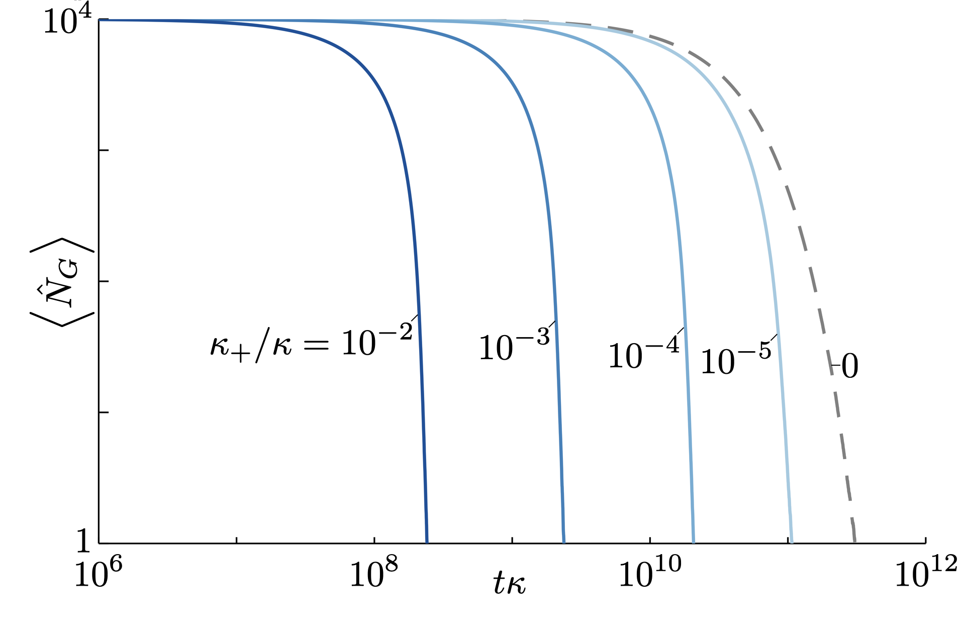
To check the validity of our adiabatic elimination, we initially compare our results to a numerical simulation of the full master equation (3) for a small system. For this simulation we also use a quantum trajectory approach Daley 2014. In Fig. 2 we compare the results for $N=8$. We find that for typical parameters, the elimination condition $\langle\hat{N}_{e}\rangle\ll 1$ is fulfilled and both descriptions match even for the largest considered cavity drive that we consider, $\kappa_{+}/\kappa=10^{-2}$. Note that when varying $N$, to make small and large system sizes comparable we approximately match the collective cavity coupling $g_{c}=\sqrt{N}g$ and pumping rate $N\Gamma_{+}$ (instead of $g$ and $\Gamma_{+}$). In this way we achieve an equivalent mixing of photons and excited states and equivalent total incoherent transfer rates.

The algorithm to compute $\langle\hat{N}_{G}\rangle$ from Eq. (22) scales only linearly with the number of pairs, which allows us to consider $N=10^{4}$ pairs in Fig. 3. In this figure we show the time evolution of the number of ground state donor-acceptor pairs for different values of $\kappa_{+}$. We observe that a weak cavity pump of only $\kappa_{+}/\kappa=10^{-5}$ already leads to a significant acceleration of the ground-state depletion at times when only few ground-state pairs remain coupled to the cavity. While the initial dynamics is barely modified, we find that the long-time depletion becomes even super-exponential. For larger values of $\kappa_{+}/\kappa$, also the earlier dynamics speeds up. For example increasing $\kappa_{+}/\kappa$ from $10^{-3}$ to $10^{-2}$, the entire dynamics shifts by a factor of $10$, indicating that the transfer is completely dominated by the cavity in this regime, as the transfer rate $r$ is proportional to the rate at which the cavity is pumped $\kappa_{+}$.

In this subsection, we analyze the dependence of the transfer rate $r$ given by Eq. (22) on the various model parameters, and identify for which parameters the presence of a cavity increases $r$. Fig. 4(a) to (c) are contour plots of the rate modification due to the cavity: $r_{\rm cav}/r_{\rm bare}$, where $r_{\rm cav}$ is given by setting $\Gamma_{+}=0$ in Eq. (22), and $r_{\rm bare}$ is given by setting $\kappa_{+}=0$ and $g=0$ in Eq. (22), describing transfer via the cavity only and without the cavity, respectively. The white lines in Fig. 4 highlight parameter points where $r_{\rm cav}=r_{\rm bare}$, i.e. where both setups perform equally well. We set $\kappa_{+}/\kappa=\Gamma_{+}/\Gamma=10^{-3}$ for both scenarios to compare situations with the same driving field: If interaction with the background photon field is the dominant loss and excitation mechanism, we have $\kappa_{+}/\kappa=\langle\hat{n}_{\rm ph}\rangle/(1+\langle\hat{n}_{\rm ph}\rangle)=\Gamma_{+}/\Gamma$, for $\langle\hat{n}_{\rm ph}\rangle$ the average photon density in the background field. This can be shown by a standard derivation of the master equation Cohen-Tannoudji, Dupont-Roc, and Grynberg 2008. Here we analyze the experimentally relevant limit (see Sec. II.2), where $\kappa\gg\Gamma$, and thus $\kappa_{+}\gg\Gamma_{+}$. Note that in an opposite limit, the bare transfer would dominate over the one via the cavity.

In all contour plots we can see that for vanishing cavity coupling $g_{c}=\sqrt{N}g\rightarrow 0$, the cavity transfer rate vanishes $r_{\rm cav}\rightarrow 0$. This happens because for $g_{c}=0$, photons cannot be transformed into donor states $\ket{D}$, and thus cannot drive any population transfer. Similarly, for diverging coupling $g_{c}\rightarrow\infty$, $r_{\rm cav}$ also vanishes, because both upper and lower polariton states [i.e. eigenstates of the second line of Eq. (2), $\ket{P_\pm}$ in Fig. 1(c)] are far detuned from the state $\ket{A}$. This suppresses coherent population transfer from the polariton states to $\ket{A}$. Between both extreme cases, we find an optimal value of $g_{c}$, for which $r_{\rm cav}$ is maximal and the cavity enhances the transfer. Notably, for a large parameter regime, the optimal $g_{c}$ lies in the weak coupling regime $g_{c}\leq\kappa/4$, a regime where the polariton splitting is not observable ²² 2 $g_{c}\leq\kappa/4$ is the condition for having two eigenstates with different eigenenergies However, the difference can be only spectrally resolved at a larger $g_{c}$. Note also that we neglected other dissipation $\Gamma,\eta\ll\kappa$, in this approximate condition..

For which parameters weak or strong coupling is optimal is e.g. seen in Fig. 4(a), which shows $r_{\rm cav}/r_{\rm bare}$ as a function of $\kappa$ and $g_{c}$ in normalized units $\kappa_{0}$. In the limit of small $\kappa$, the enhancement is maximal for a collective coupling strength matching the energy difference between states $\ket{A}$ and $\ket{D}$, $g_{c}\sim\Delta=0.2\kappa_{0}$. This can be understood from taking the limit $V\to 0$ in the Hamiltonian Eq. (2). Then, $\ket{A}$ is in resonance with an upper polariton state [$\ket{P_+}$ in Fig. 1(c)] of the Tavis-Cummings part [second line in Eq. (2)]. We thus find that in this strong coupling limit, the enhancement is efficiently mediated by a polaritonic state. In contrast, for larger values of $\kappa$, $r_{\rm cav}$ is maximal for a $g_{c}$ inside the weak coupling regime. There, although no polariton splitting is present, the mixing between cavity and donor state induced by the non-hermitian Hamiltonian (9) can still be important. Thus, there is an excited state with both cavity and $\ket{A}$ state contribution which can enable coherent transfer, although in many cases the cavity photon decays before this coherent transfer takes place. For a given $g_{c}$ there exists an optimal finite $\kappa>0$. This optimal $\kappa$ is larger than zero, since in the limit $\kappa\rightarrow 0$ the cavity cannot be excited by the incoherent pump. In the limit $\kappa\rightarrow\infty$, the cavity photons are lost before they can be absorbed by a donor-acceptor pair. We find that lines of constant enhancement correspond to $g_{c}\propto\sqrt{\kappa}$, indicating that the proper figure of merit is the collective Purcell factor $g_{c}^{2}/\kappa$, which is not tied to weak or strong coupling.

Similar effects can be observed for variable energy difference between the states $\ket{D}$ and $\ket{A}$ in Fig. 4(b), which shows $r_{\rm cav}/r_{\rm bare}$ as a function of $\Delta$ and $g_{c}$. For large $\Delta$, the transfer efficiency is maximal for $g_{c}\approx|\Delta|$. We again attribute these points of efficient populations transfer to respective resonances with the upper and lower polariton states of the Tavis-Cummings part in the Hamiltonian. For larger $g_{c}\gg|\Delta|$, the large detuning leads to a large suppression of the transfer rate, as both polaritons are out of resonance. In contrast, for small values of $|\Delta|$, $r_{\rm cav}/r_{\mathrm{bare}}$ is maximal for a small $g_{c}$ close to the weak coupling regime. Note that we still find significant cavity enhancement inside this weak coupling regime.

In Fig. 4(c) we analyze $r_{\rm cav}/r_{\rm bare}$ as function of $g$ and $N$. Here, we find that increasing $N$ decreases the cavity enhancement factor $r_{\rm cav}/r_{\rm bare}$, although it increases the collective cavity coupling $g_{c}$. Fig. 4(d) is a cut through Fig. 4(c) for fixed $g$. For increasing $N$, initially the collective effects increase the cavity transfer rate $r_{\rm cav}$. However, this effect competes with an increase of $r_{\rm bare}\propto N$ due to the increasing number of transfer channels. For small $N$, the collective effects compensate for the increasing number of transfer channels, keeping $r_{\rm cav}/r_{\rm bare}$ approximately constant. This can also be seen as vertical sections of contours in Fig. 4(c) for small $g$. Further increasing $N$, the collective enhancement becomes weaker and $r_{\rm cav}/r_{\rm bare}$ decreases. For $g_{c}\gtrsim(\kappa,\Delta)$, $r_{\rm cav}$ decreases for increasing $N$ due to a too large polariton splitting. Note that here $N$ is the number of pairs in state $\ket{G}$, such that even if initially the enhancement is only weak, at later times a larger enhancement can be observed [see also Fig. 3].

In the analysis of Fig. 4 we found that the main features of the cavity modification of initial transfer rates can be understood in terms of resonance conditions of collective bright states, which is included in the state overlaps [compare Fig. 1(c)]. It is important to point out that in general the dynamics can also involve dark states, populated through individual pumping. Therefore, lastly we also analyze the instantaneous rates with both cavity ($\kappa_{+}>0$) and individual pair ($\Gamma_{+}>0$) pumping. To distinguish a scaling in the number of pairs $N$ from simple polaritonic resonance conditions, we now compare rates as function of the collective cavity coupling, $g_{c}=g\sqrt{N}$ and $N$ in Fig. 5. In general, we now find that, depending on $g_{c}$, for large enough $N$, the overall instantaneous transfer rate $r_{\rm tot}$ exhibits a dependence on $N$ [Fig. 5(a)]. This can be explained by a dominance of dark state transfer for large $N$ [as sketched in Fig. 1(d)]. This is exemplified in Fig. 5(b), where we compare the contributions to $r_{\rm tot}=r_{\rm cav}+r_{\mathrm{ind}}$, which besides the cavity rate $r_{\rm cav}$ now also contains the bare individual pumping part $r_{\mathrm{ind}}$. We define the latter by setting $\kappa_{+}=0$ in Eq. (22), which is different from $r_{\rm bare}$ which is defined outside the cavity by setting $g=\kappa_{+}=0$. Note that in accordance with the discussion above, $r_{\mathrm{cav}}$ does not depend on $N$ for constant $g_{c}$, whereas $r_{\mathrm{ind}}$ grows with increasing $N$. We find that for large enough $N$, $r_{\rm tot}$ is dominated by $r_{\mathrm{ind}}$. Furtheremore, for large $N$, the cavity influence on the individual pumping vanishes and $r_{\mathrm{ind}}\approx r_{\mathrm{bare}}$. This can be understood from the fact that the states excited by $\Gamma_{+}$ have vanishing polariton contribution [$c^{D_{n}}_{\pm,X}\rightarrow 0$ as $N\rightarrow\infty$ in Eq. (22)], and in our model the dark states $\ket{k_\pm}$ decouple from the cavity. Note that in the regime of small $N$, where individual pumping excites a significant fraction of bright states, we find $r_{\mathrm{ind}}<r_{\mathrm{bare}}$.

It is worth to re-emphasize that the dynamics is governed by a non-linear rate equation, which implies that the instantaneous rate from Eq. (22) also depends on time. Then, the time dependence of resonance conditions, together with the dependence on rates on $N$ due to bright and dark state contributions from Fig. 5, give rise to non-trivial decay dynamics, as the super-exponential behavior observed in Fig. 3.

Finally, we want to emphasize that we conclude from Fig. 4, that for the numbers relevant for nanocrystal setups as described in Sec. II.2, the initial transfer rate can be enhanced by a factor $r_{\rm cav}/r_{\rm bare}\sim 2.5$ in the cavity-coupled scenario.

References

- Ebbesen (2016) T. W. Ebbesen, “Hybrid light–matter states in a molecular and material science perspective,” Acc. Chem. Res. 49, 2403–2412 (2016).
- Herrera and Owrutsky (2020) F. Herrera and J. Owrutsky, “Molecular polaritons for controlling chemistry with quantum optics,” J. Chem. Phys. 152, 100902 (2020).
- Thomas et al. (2016) A. Thomas, J. George, A. Shalabney, M. Dryzhakov, S. J. Varma, J. Moran, T. Chervy, X. Zhong, E. Devaux, C. Genet, J. A. Hutchison, and T. W. Ebbesen, “Ground-State Chemical Reactivity under Vibrational Coupling to the Vacuum Electromagnetic Field,” Angew. Chem. Int. Ed. 55, 11462 (2016).
- Dunkelberger et al. (2016) A. D. Dunkelberger, B. T. Spann, K. P. Fears, B. S. Simpkins, and J. C. Owrutsky, “Modified relaxation dynamics and coherent energy exchange in coupled vibration-cavity polaritons,” Nat. Commun. 7, 1–10 (2016).
- Thomas et al. (2019) A. Thomas, L. Lethuillier-Karl, K. Nagarajan, R. M. A. Vergauwe, J. George, T. Chervy, A. Shalabney, E. Devaux, C. Genet, J. Moran, and T. W. Ebbesen, “Tilting a ground-state reactivity landscape by vibrational strong coupling,” Science 363, 615–619 (2019).
- Lather et al. (2019) J. Lather, P. Bhatt, A. Thomas, T. W. Ebbesen, and J. George, “Cavity Catalysis by Cooperative Vibrational Strong Coupling of Reactant and Solvent Molecules,” Angew. Chem. Int. Ed. 58, 10635–10638 (2019).
- Hiura, Shalabney, and George (2019) H. Hiura, A. Shalabney, and J. George, “Vacuum-Field Catalysis: Accelerated Reactions by Vibrational Ultra Strong Coupling,” figshare (2019), 10.26434/chemrxiv.7234721.v4.
- Hutchison et al. (2012) J. A. Hutchison, T. Schwartz, C. Genet, E. Devaux, and T. W. Ebbesen, “Modifying Chemical Landscapes by Coupling to Vacuum Fields,” Angew. Chem. Int. Ed. 51, 1592–1596 (2012).
- Munkhbat et al. (2018) B. Munkhbat, M. Wersäll, D. G. Baranov, T. J. Antosiewicz, and T. Shegai, “Suppression of photo-oxidation of organic chromophores by strong coupling to plasmonic nanoantennas,” Sci. Adv. 4, eaas9552 (2018).
- Peters et al. (2019) V. N. Peters, M. O. Faruk, J. Asane, R. Alexander, D. A. Peters, S. Prayakarao, S. Rout, and M. A. Noginov, “Effect of strong coupling on photodegradation of the semiconducting polymer P3HT,” Optica 6, 318–325 (2019).
- Herrera and Spano (2016) F. Herrera and F. C. Spano, “Cavity-controlled chemistry in molecular ensembles,” Phys. Rev. Lett. 116, 238301 (2016).
- Kowalewski, Bennett, and Mukamel (2016) M. Kowalewski, K. Bennett, and S. Mukamel, “Cavity femtochemistry: Manipulating nonadiabatic dynamics at avoided crossings,” J. Phys. Chem. Lett. 7, 2050–2054 (2016).
- Flick et al. (2017) J. Flick, M. Ruggenthaler, H. Appel, and A. Rubio, “Atoms and molecules in cavities, from weak to strong coupling in quantum-electrodynamics (QED) chemistry,” Proc. Natl. Acad. Sci. U.S.A. 114, 3026–3034 (2017).
- Feist, Galego, and Garcia-Vidal (2018) J. Feist, J. Galego, and F. J. Garcia-Vidal, “Polaritonic chemistry with organic molecules,” ACS Photonics 5, 205–216 (2018).
- Flick and Narang (2018) J. Flick and P. Narang, “Cavity-Correlated Electron-Nuclear Dynamics from First Principles,” Phys. Rev. Lett. 121, 113002 (2018).
- Vendrell (2018) O. Vendrell, “Collective Jahn-Teller interactions through light-matter coupling in a cavity,” Phys. Rev. Lett. 121, 253001 (2018).
- Campos-Gonzalez-Angulo, Ribeiro, and Yuen-Zhou (2019) J. A. Campos-Gonzalez-Angulo, R. F. Ribeiro, and J. Yuen-Zhou, “Resonant catalysis of thermally activated chemical reactions with vibrational polaritons,” Nat. Commun. 10, 1–8 (2019).
- Fregoni et al. (2020) J. Fregoni, G. Granucci, M. Persico, and S. Corni, “Strong Coupling with Light Enhances the Photoisomerization Quantum Yield of Azobenzene,” Chem 6, 250–265 (2020).
- Herrera (2020) F. Herrera, “Photochemistry with Quantum Optics from a Non-Adiabatic Quantum Trajectory Perspective,” Chem 6, 7–9 (2020).
- Ulusoy and Vendrell (2020) I. S. Ulusoy and O. Vendrell, “Dynamics and spectroscopy of molecular ensembles in a lossy microcavity,” J. Chem. Phys. 153, 044108 (2020).
- Felicetti et al. (2020) S. Felicetti, J. Fregoni, T. Schnappinger, S. Reiter, R. de Vivie-Riedle, and J. Feist, “Photoprotecting Uracil by Coupling with Lossy Nanocavities,” J. Phys. Chem. Lett. 11, 8810–8818 (2020).
- Wang et al. (2020) D. S. Wang, T. Neuman, J. Flick, and P. Narang, “Weak-to-Strong Light-Matter Coupling and Dissipative Dynamics from First Principles,” arXiv (2020), 2002.10461 .
- Antoniou et al. (2020) P. Antoniou, F. Suchanek, J. F. Varner, and J. J. F. I. V., “Role of Cavity Losses on Nonadiabatic Couplings and Dynamics in Polaritonic Chemistry,” J. Phys. Chem. Lett. 11, 9063–6069 (2020).
- Kowalewski and Davidsson (2020) M. Kowalewski and E. Davidsson, “Simulating photodissociation reactions in bad cavities with the lindblad equation,” J. Chem. Phys. 153, 234304 (2020).
- Torres-Sánchez and Feist (2021) J. Torres-Sánchez and J. Feist, “Molecular Photodissociation enabled by Ultrafast Plasmon Decay,” J. Chem. Phys 154, 014303 (2021).
- Herrera and Spano (2017) F. Herrera and F. C. Spano, “Theory of Nanoscale Organic Cavities: The Essential Role of Vibration-Photon Dressed States,” ACS Photonics 5, 65–79 (2017).
- del Pino, Feist, and Garcia-Vidal (2015) J. del Pino, J. Feist, and F. J. Garcia-Vidal, “Quantum theory of collective strong coupling of molecular vibrations with a microcavity mode,” New J. Phys. 17, 053040 (2015).
- Martínez-Martínez et al. (2018) L. A. Martínez-Martínez, M. Du, R. F. Ribeiro, S. Kéna-Cohen, and J. Yuen-Zhou, “Polariton-assisted singlet fission in acene aggregates,” J. Phys. Chem. Lett. 9, 1951–1957 (2018).
- Reitz, Sommer, and Genes (2019) M. Reitz, C. Sommer, and C. Genes, “Langevin Approach to Quantum Optics with Molecules,” Phys. Rev. Lett. 122, 203602 (2019).
- Finkelstein-Shapiro et al. (2020) D. Finkelstein-Shapiro, D. Viennot, I. Saideh, T. Hansen, T. Pullerits, and A. Keller, “Adiabatic elimination and subspace evolution of open quantum systems,” Phys. Rev. A 101, 042102 (2020).
- Reiter and Sørensen (2012) F. Reiter and A. S. Sørensen, “Effective operator formalism for open quantum systems,” Phys. Rev. A 85, 032111 (2012).
- Wellnitz et al. (2020) D. Wellnitz, S. Schütz, S. Whitlock, J. Schachenmayer, and G. Pupillo, “Collective Dissipative Molecule Formation in a Cavity,” Phys. Rev. Lett. 125, 193201 (2020).
- Jin and Ye (2012) D. S. Jin and J. Ye, “Introduction to Ultracold Molecules: New Frontiers in Quantum and Chemical Physics,” Chem. Rev. 112, 4801–4802 (2012).
- Dulieu and Osterwalder (2017) O. Dulieu and A. Osterwalder, Cold Chemistry (The Royal Society of Chemistry, 2017).
- Mandal, Krauss, and Huo (2020) A. Mandal, T. D. Krauss, and P. Huo, “Polariton-Mediated Electron Transfer via Cavity Quantum Electrodynamics,” J. Phys. Chem. B 124, 6321–6340 (2020).
- Ulusoy, Gomez, and Vendrell (2019) I. S. Ulusoy, J. A. Gomez, and O. Vendrell, “Modifying the Nonradiative Decay Dynamics through Conical Intersections via Collective Coupling to a Cavity Mode,” J. Phys. Chem. A 123, 8832–8844 (2019).
- Szidarovszky, Halász, and Vibók (2020) T. Szidarovszky, G. J. Halász, and Á. Vibók, “Three-player polaritons: nonadiabatic fingerprints in an entangled atom–molecule–photon system,” New J. Phys. 22, 053001 (2020).
- Davidsson and Kowalewski (2020) E. Davidsson and M. Kowalewski, “Atom Assisted Photochemistry in Optical Cavities,” J. Phys. Chem. A 124, 4672–4677 (2020).
- Gonzalez-Ballestero et al. (2016) C. Gonzalez-Ballestero, J. Feist, E. Gonzalo Badía, E. Moreno, and F. J. Garcia-Vidal, “Uncoupled Dark States Can Inherit Polaritonic Properties,” Phys. Rev. Lett. 117, 156402 (2016).
- Groenhof et al. (2019) G. Groenhof, C. Climent, J. Feist, D. Morozov, and J. J. Toppari, “Tracking Polariton Relaxation with Multiscale Molecular Dynamics Simulations,” J. Phys. Chem. Lett. 10, 5476–5483 (2019).
- Sommer et al. (2020) C. Sommer, M. Reitz, F. Mineo, and C. Genes, “Molecular polaritonics in dense mesoscopic disordered ensembles,” arXiv (2020), 2010.07155 .
- Botzung et al. (2020) T. Botzung, D. Hagenmüller, S. Schütz, J. Dubail, G. Pupillo, and J. Schachenmayer, “Dark state semilocalization of quantum emitters in a cavity,” Phys. Rev. B 102, 144202 (2020).
- Chávez et al. (2020) N. C. Chávez, F. Mattiotti, J. A. Méndez-Bermúdez, F. Borgonovi, and G. L. Celardo, “Disorder-Enhanced and Disorder-Independent Transport with long-range hopping: application to molecular chains in optical cavities,” arXiv (2020), 2010.08060 .
- (44) Precisely, the rotating frame transformation is achieved by applying the unitary operator , where the Hamiltonian and the states transform according to and , respectively.
- Gardiner and Zoller (2004) C. Gardiner and P. Zoller, Quantum noise: a handbook of Markovian and non-Markovian quantum stochastic methods with applications to quantum optics (Springer Science & Business Media, 2004).
- Zhu et al. (2014) H. Zhu, Y. Yang, K. Hyeon-Deuk, M. Califano, N. Song, Y. Wang, W. Zhang, O. V. Prezhdo, and T. Lian, “Auger-Assisted Electron Transfer from Photoexcited Semiconductor Quantum Dots,” Nano Lett. 14, 1263–1269 (2014).
- Gupta and Waks (2013) S. Gupta and E. Waks, “Spontaneous emission enhancement and saturable absorption of colloidal quantum dots coupled to photonic crystal cavity,” Opt. Express 21, 29612–29619 (2013).
- Misra and Sudarshan (1977) B. Misra and E. C. G. Sudarshan, “The Zeno’s paradox in quantum theory,” J. Math. Phys. 18, 756–763 (1977).
- Zeb, Kirton, and Keeling (2018) M. A. Zeb, P. G. Kirton, and J. Keeling, “Exact states and spectra of vibrationally dressed polaritons,” ACS Photonics 5, 249–257 (2018).
- del Pino et al. (2018) J. del Pino, F. A. Y. N. Schröder, A. W. Chin, J. Feist, and F. J. Garcia-Vidal, “Tensor Network Simulation of Non-Markovian Dynamics in Organic Polaritons,” Phys. Rev. Lett. 121, 227401 (2018).
- Gardiner et al. (1985) C. W. Gardiner et al., Handbook of stochastic methods, Vol. 3 (springer Berlin, 1985).
- Sakurai and Napolitano (2021) J. J. Sakurai and J. Napolitano, Modern quantum mechanics, 3rd edition (Cambridge University Press, 2021).
- Daley (2014) A. J. Daley, “Quantum trajectories and open many-body quantum systems,” Adv. Phys. 63, 77–149 (2014).
- Cohen-Tannoudji, Dupont-Roc, and Grynberg (2008) C. Cohen-Tannoudji, J. Dupont-Roc, and G. Grynberg, “Radiation considered as a reservoir: Master equation for the particles,” in Atom—Photon Interactions (John Wiley & Sons, Ltd, 2008) Chap. 4, pp. 257–351.
- (55) is the condition for having two eigenstates with different eigenenergies However, the difference can be only spectrally resolved at a larger . Note also that we neglected other dissipation , in this approximate condition.
- Atwater and Polman (2010) H. A. Atwater and A. Polman, “Plasmonics for improved photovoltaic devices,” Nat. Mater. 9, 205–213 (2010).
- Ikeda et al. (2011) K. Ikeda, K. Takahashi, T. Masuda, and K. Uosaki, “Plasmonic Enhancement of Photoinduced Uphill Electron Transfer in a Molecular Monolayer System,” Angew. Chem. Int. Ed. 50, 1280–1284 (2011).
- Zhang et al. (2013) X. Zhang, Y. L. Chen, R.-S. Liu, and D. P. Tsai, “Plasmonic photocatalysis,” Rep. Prog. Phys. 76, 046401 (2013).
- Coles et al. (2014) D. M. Coles, N. Somaschi, P. Michetti, C. Clark, P. G. Lagoudakis, P. G. Savvidis, and D. G. Lidzey, “Polariton-mediated energy transfer between organic dyes in a strongly coupled optical microcavity,” Nat. Mater. 13, 712–719 (2014).
- Zhong et al. (2016) X. Zhong, T. Chervy, S. Wang, J. George, A. Thomas, J. A. Hutchison, E. Devaux, C. Genet, and T. W. Ebbesen, “Non-Radiative Energy Transfer Mediated by Hybrid Light-Matter States,” Angew. Chem. Int. Ed. 55, 6202–6206 (2016).
- Zhong et al. (2017) X. Zhong, T. Chervy, L. Zhang, A. Thomas, J. George, C. Genet, J. A. Hutchison, and T. W. Ebbesen, “Energy Transfer between Spatially Separated Entangled Molecules,” Angew. Chem. Int. Ed. 56, 9034 (2017).
- Stranius, Hertzog, and Börjesson (2018) K. Stranius, M. Hertzog, and K. Börjesson, “Selective manipulation of electronically excited states through strong light–matter interactions,” Nat. Commun. 9, 1–7 (2018).
- Takahashi, Watanabe, and Matsumoto (2019) S. Takahashi, K. Watanabe, and Y. Matsumoto, “Singlet fission of amorphous rubrene modulated by polariton formation,” J. Chem. Phys. 151, 074703 (2019).
- Eizner et al. (2019) E. Eizner, L. A. Martínez-Martínez, J. Yuen-Zhou, and S. Kéna-Cohen, “Inverting singlet and triplet excited states using strong light-matter coupling,” Sci. Adv. 5, eaax4482 (2019).
- Yu et al. (2020) Y. Yu, S. Mallick, M. Wang, and K. Börjesson, “Barrier-Free Reverse-Intersystem Crossing by Strong Light-Matter Coupling,” figshare (2020), 10.26434/chemrxiv.12932972.v1.
- Polak et al. (2020) D. Polak, R. Jayaprakash, T. P. Lyons, L. Á. Martínez-Martínez, A. Leventis, K. J. Fallon, H. Coulthard, D. G. Bossanyi, K. Georgiou, I. I. Anthony J. Petty, J. Anthony, H. Bronstein, J. Yuen-Zhou, A. I. Tartakovskii, J. Clark, and A. J. Musser, “Manipulating molecules with strong coupling: harvesting triplet excitons in organic exciton microcavities,” Chem. Sci. 11, 343–354 (2020).
- (67) See https://www.wolframalpha.com/input/?i=%7B%7Bd0%2C+sqrt%7BM%7D*g%2C+0%7D%2C+%7Bsqrt%7BM%7D*g%2C+d1%2C+V%7D%2C+%7B0%2C+V%2C+d2%7D%7D for the full expression.