Elisa Garcia Pereira
Ground Level Muon Flux Variation in a Cosmic Rays SimulationPublication type: Article Type
Abstract
The oscillatory movements of atmospheric air masses has been claimed to be the origin of the muon flux variation measured at the ground level. Using a cosmic ray toolkit (CORSIKA), we simulate cascade scenarios in a time scale of a year and show the dependence of the muon flux pattern with a proposed oscillatory model atmosphere.
keywords
Cosmic rays, CORSIKA, atmospheric tides1 Introduction
High energy cosmic rays, mostly protons, but also alpha particles and heavy nucleus, hit the air molecules starting an extensive air shower. A shower is a cascade of many kilometers of ionized particles and electromagnetic radiation. As the fragments of the first collision hit other nuclei, a cascade of pions is produced. The neutral pions initiate an electromagnetic shower constituted of photons, electrons and positrons. The charged pions will interact with other atoms or in turn, decay into muons and neutrinos, constituting the most prominent flux at the ground level.
The role played by the atmosphere is that of a giant calorimeter, where the ground level flux is stongly dependent on the atmospheric density. There are several mechanisms that lead to changes in atmospheric density. For example, solar heating of atmospheric layers is the dominant mechanism, that gives origin to atmospheric tides (Lindzen \BBA Chapman \APACyear1970; Lindzen \APACyear1967; Lindzen \APACyear1979; Lindgren \APACyear1962). These tides are oscillatory movements of air masses characterized by a set of accurately known frequencies that reflect the amount of daily insolation as Earth revolves around the Sun. In principle these air density tides could effect the muon flux at the ground level. In the experiment performed by Takai and collaborators they report the detection of tidal frequencies in the spectral analysis of time series muon flux measurements realized over a period of eight years (Takai \BBA et al. \APACyear2016).
An alternative approach to the direct measurement of cosmic rays has been the development of powerful simulation tools, based on Monte Carlo techniques that incorporate the complex physical content of the extensive air shower. In particular, the CORSIKA (COsmic Ray SImulations for KAscade) toolkit is a code for detailed simulation of these showers that are initiated by high energy cosmic ray particles. It allows one to study the interactions and decay of nucleus, hadrons, muons, electrons, and photons of high energy, over eV, in the atmosphere (CORSIKA \APACyear2020).
In this work, we shall examine the periodic variation of the atmospheric density as an influence on the muon flux counting at the ground level, using the CORSIKA toolkit simulations. Our main objective is to compare the simulated results with experimental data that exhibits a tidal frequency behavior.
2 Muon flux measurement
In this section we shall briefly review the muon detection experiment of reference (Takai \BBA et al. \APACyear2016), that reports the detection of tidal frequencies in the spectral analysis of time series muon flux measurements realized over a period of eight years. The muon telescope used for these measurements was part of the MARIACHI experiment, located at Smithtown High School East in the state of New York, latitude 40∘ 52’ 14.88”N, longitude 73∘ 9’ 53.103”W and 43 m above sea level. The large-scale oscillations of the atmosphere, producing tides are those, in general, generated by (a) the gravitational forces of the moon and sun, and (b) the thermal action of the sun (Lindzen \BBA Chapman \APACyear1970).
The detection system consisted of two 0.28 m2 plastic scintillators subtending a solid angle of 3.8 sr. Counts per minute were recorded by a computer and assigned a time stamp provided by a GPS clock with a nominal accuracy of 100 ns. The setup was located indoors with approximately 19 g/cm2 of roofing material above the detectors. The muons were detected with momenta above 200 MeV/c. They recorded a total number of samples of . The average measured muon rate was (1890 51) counts/min, which corresponds to a rate of 29.6 0.8 counts/s m2 sr.
Figure 1 is extracted from (Takai \BBA et al. \APACyear2016) where an hourly-averaged, pressure corrected time series of muon data is seen. A striking feature is a yearly modulation with an amplitude of 5% of the average counts, with maxima and minima during winter and summer seasons, respectively. This modulation is caused by seasonal variations in solar heating that expand or contract the atmosphere. This change in atmospheric thickness alters, increasing or decreasing, the muon flight path.
3 The Numerical Model
To simulate a similar effect, as the experiment described in the last section, we used the CORSIKA toolkit (version 7100), which is a detailed Monte Carlo program designed to study the evolution of extensive air showers in the atmosphere initiated by photons, protons, nuclei, or any other particle. It was originally developed to perform simulations for the KASCADE experiment (Doll \BBA et al. \APACyear1990; Klages \APACyear1997) at Karlsruhe and has been refined over the past years. The program recognizes 50 elementary particles: , , , , , , , ; the baryons p, n, , , , , , , the corresponding anti-baryons, the resonance states , , , , , , , , and the corresponding anti-baryonic resonances. Optionally the neutrinos and and anti-neutrinos and resulting from , , and decay may be generated explicitly. In addition nuclei up to A = 56 can also be treated.
To adapt CORSIKA’s code for our problem, first we changed its execution parameters in an automated way, by creating simple auxiliary codes in bash, Python 3, C, and R. We assume that the primary particle is always a proton with an energy of 10 TeV. In order to compare with Fig. 1, our simulation is set for New York, choosing the local magnetic field (NOAA \APACyear2020) and placing the detector m above sea level, as is described in (Takai \BBA et al. \APACyear2016). Our simulation is for a time span of one year. To improve the numerical performance, the seed of each run is random and the final data is the averaged over five runs with the same parameters but different seeds. The atmospheric data was extracted from CORSIKA’s documentation and the magnetic field parameters from the NOAA’s website (NOAA \APACyear2020).

A crucial step in our calculation is the definition of the atmospheric model. CORSIKA adopts the Earth’s atmospheric composition as N2, O2, Ar and its density variation is modeled by 5 layers. In the four lower layers, the density function has an exponential dependence with the height , while a linear dependence in the fifth layer:
| (1a) | |||||
| (1b) | |||||
All layers are parameterized by coefficients , and with , defined in table 3, where we adopt the U.S. standard atmosphere, as is presented in the CORSIKA documentation.
In order to incorporate the oscillatory movements of atmospheric air masses we must modify the density function , with the inclusion of a periodic time dependence in the four lower layers by the following substitution
| (2) |
with . We have chosen the same time dependent function for all the coefficients and assume
| (3) |
where is , is measured in days and is a free parameter. The original CORSIKA atmosphere is regained by setting the phenomenological parameter in (3). A plot of the new is seen in Fig Results with four different values and at a height of km.
| (km) | (g/cm2) | (g/cm2) | (g/cm2) | |
| 1 | 0-4 | -186.555305 | 1222.6562 | 994186.38 |
| 2 | 4-10 | -94.919 | 1144.9069 | 878153.55 |
| 3 | 10-40 | 0.61289 | 1305.5948 | 636143.04 |
| 4 | 40-100 | 0 | 540.1778 | 772170.16 |
| 5 | 100 | 0.01128292 | 1 | 10000000000 |
tableParameters of the U.S. standard atmosphere
Results
In Fig. Results is shown the simulation for the number of muons per day in a year for different values. The behavior is consistent with the results presented in Fig Results, where an increase in implies a decrease in the number of muons, in the middle of the year (when is maximum). These results are in agreement with an annual measurement seen in Fig. 1
![[Uncaptioned image]](2011.06480v1/th.png) \captionof
\captionof
figureThe model atmospheric density function
![[Uncaptioned image]](2011.06480v1/sinwt_hours.png) \captionof
\captionof
figureMuon counts over a period of a year, for different values
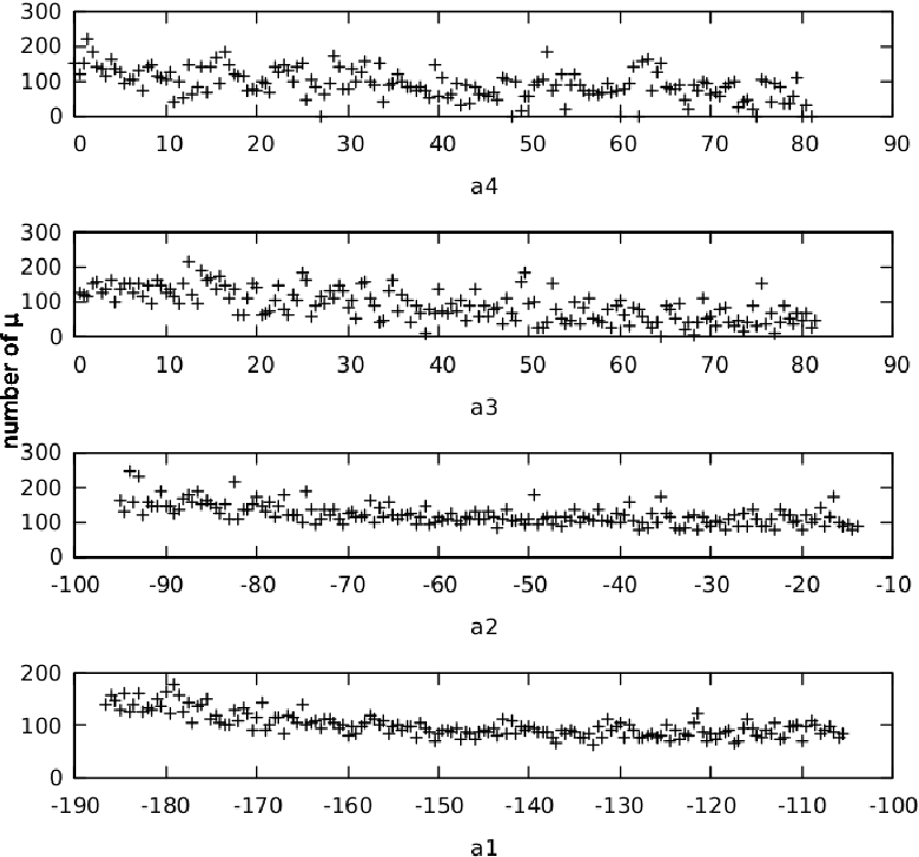
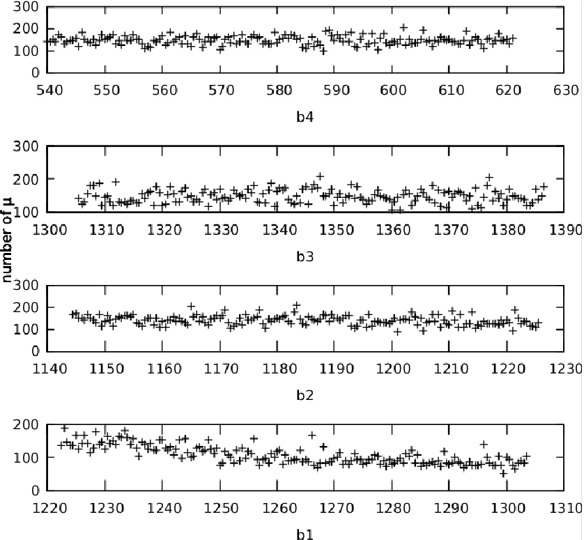
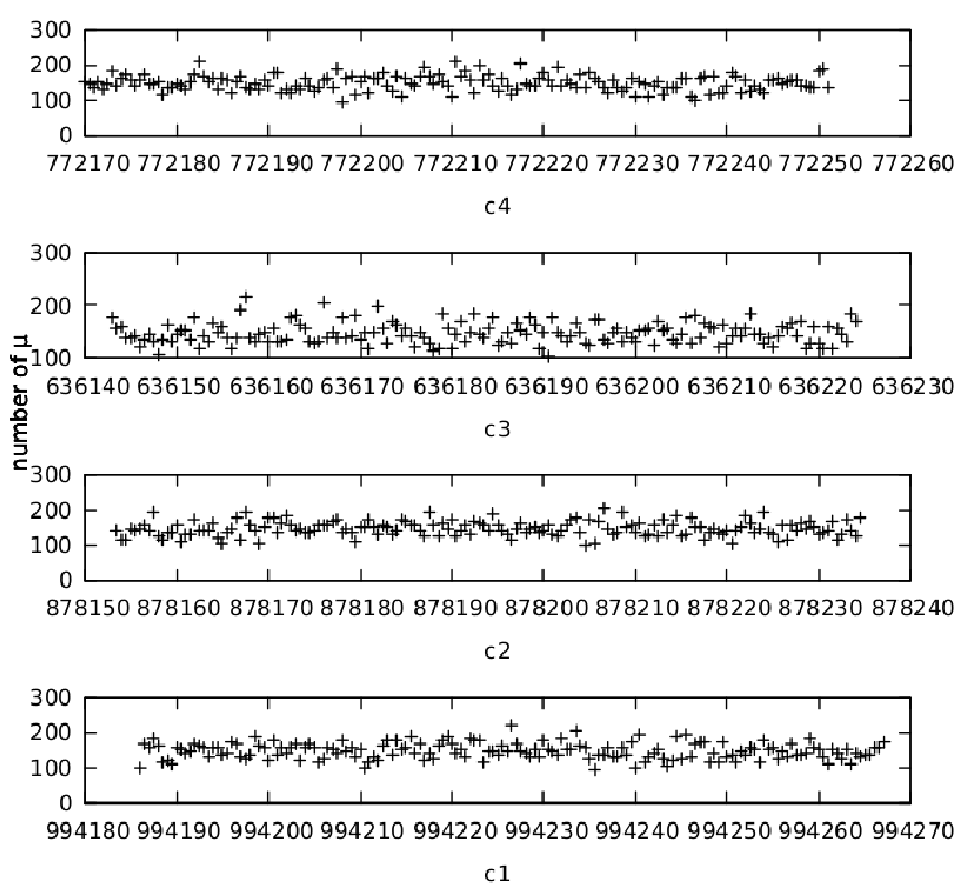
To test the sensibility of this effect in each atmospheric layer, figures 2- 4 are plots of muon counts while varing parameters , and . The strategy is to keep all the other parameters constant, according to table 3, as we change, with a simple linear variation, each parameter individually. For the sake of comparison we choose the case g/cm2 in Figures Results and Results . Therefore each parameter starts from the original tabulated value, increased with a step of 0.5 g/cm2, stopping when the sum of the increments add up to 81 g/cm2. In the lowst atmospheric layer (), from ground level up to 4 km, more muons are detected for smaller parameter values, as seen in figures 2 and 3 for and , respectively. Which means that in the layer closer to the ground level, the weight is more influential. For the other values we still have a slow and subtle decrease in the number of muons detected on the ground level. As for the other values no significant change in the number of muons is present for the upper atmospheric layers. The same conclusion is valid for all the values calculated.
4 Conclusions
Notwithstanding the simulation was restricted to the range of a year, due to computation time, it is clear that, for the chosen atmospheric density range, the lower layers are more influential on the number of muons. We have also shown that a simple phenomenological periodic time-dependent density function can reproduce qualitatively the complex atmospheric tides effects that are revealed in the muon data.
We aim in our forthcoming research to explore more realistic atmospheric models, based on the theory of atmospheric and thermal tides. This investigation can provide the sources of periodic excitation and atmospheric response to the excitation.
References
- CORSIKA (\APACyear2020) \APACinsertmetastarcorsika{APACrefauthors}CORSIKA. \APACrefYearMonthDay2020, \APACrefbtitleCOsmic Ray SImulations for KAscade. COsmic Ray SImulations for KAscade., \APAChowpublishedhttps://www.ikp.kit.edu/corsika/. \PrintBackRefs\CurrentBib
- Doll \BBA et al. (\APACyear1990) \APACinsertmetastarkascade1{APACrefauthors}Doll, P.\BCBT \BBA et al. \APACrefYearMonthDay1990, \APACjournalVolNumPagesNucl. Phys. B (Proc. Suppl.)14A336. \APACrefnoteThe Karlsruhe Cosmic Ray Project KASCADE \PrintBackRefs\CurrentBib
- Klages (\APACyear1997) \APACinsertmetastarkascade2{APACrefauthors}Klages, H\BPBIO. \APACrefYearMonthDay1997, \APACjournalVolNumPagesNucl. Phys. B (Proc. Suppl.)52B92. \APACrefnoteKASCADE Collaboration \PrintBackRefs\CurrentBib
- Lindgren (\APACyear1962) \APACinsertmetastarlindgren{APACrefauthors}Lindgren, S. \APACrefYearMonthDay1962, \APACjournalVolNumPagesTellus1444. \APACrefnoteOn the pressure dependence of the cosmic ray intensity recorded by the standard neutron monitor \PrintBackRefs\CurrentBib
- Lindzen (\APACyear1967) \APACinsertmetastarlindzen2{APACrefauthors}Lindzen, R\BPBIS. \APACrefYearMonthDay1967, \APACjournalVolNumPagesQ. J. R. Meteorol. Soc.9318. \APACrefnoteThermally driven diurnal tide in the atmosphere \PrintBackRefs\CurrentBib
- Lindzen (\APACyear1979) \APACinsertmetastarlindzen3{APACrefauthors}Lindzen, R\BPBIS. \APACrefYearMonthDay1979, \APACjournalVolNumPagesAnn. Rev. Earth Planet. Sci7199. \APACrefnoteAtmospheric Tides \PrintBackRefs\CurrentBib
- Lindzen \BBA Chapman (\APACyear1970) \APACinsertmetastarlindzen1{APACrefauthors}Lindzen, R\BPBIS.\BCBT \BBA Chapman, S. \APACrefYear1970, \APACrefbtitleAtmospheric Tides Atmospheric Tides. \APACaddressPublisherSpringer. \APACrefnote978-9401034012 \PrintBackRefs\CurrentBib
- NOAA (\APACyear2020) \APACinsertmetastarmagnet{APACrefauthors}NOAA. \APACrefYearMonthDay2020, \APACrefbtitleNational Oceanic and Atmospheric Administration. National Oceanic and Atmospheric Administration., \APAChowpublishedhttps://www.ngdc.noaa.gov. \APACrefnoteMagnetic Field Calculators \PrintBackRefs\CurrentBib
- Takai \BBA et al. (\APACyear2016) \APACinsertmetastartakai{APACrefauthors}Takai, H.\BCBT \BBA et al. \APACrefYearMonthDay2016, \APACjournalVolNumPagesarXiv:1610.05983. \APACrefnoteTidal Frequencies in the Time Series Measurements of Atmospheric Muon Flux from Cosmic Rays \PrintBackRefs\CurrentBib
Acknowledgements
The authors thank the High Energy Physics Simulations group (HEPsim, www.ufrgs.br/hepsim) for all the help and discussion in high energy physics simulations.