Quantitative homogenization of
interacting particle systems
Abstract.
For a class of interacting particle systems in continuous space, we show that finite-volume approximations of the bulk diffusion matrix converge at an algebraic rate. The models we consider are reversible with respect to the Poisson measures with constant density, and are of non-gradient type. Our approach is inspired by recent progress in the quantitative homogenization of elliptic equations. Along the way, we develop suitable modifications of the Caccioppoli and multiscale Poincaré inequalities, which are of independent interest.
MSC 2010: 82C22, 35B27, 60K35.
Keywords: interacting particle system, hydrodynamic limit, quantitative homogenization.
1. Introduction
The goal of this paper is to make progress on the quantitative analysis of interacting particle systems. We consider a class of models in which each particle follows a random evolution on which is influenced by the configuration of neighboring particles. The models we consider are reversible with respect to the Poisson measures with constant density, uniformly elliptic, and of non-gradient type. For similar models in this class, the hydrodynamic limit and the equilibrium fluctuations have been identified rigorously. In both these results, the limit object is described in terms of the bulk diffusion matrix. The main result of this paper is a proof that finite-volume approximations of this diffusion matrix converge at an algebraic rate.
Our strategy is inspired by recent developments in the quantitative analysis of elliptic equations with random coefficients, and in particular on the renormalization approach developed in [14, 13, 9, 10, 11, 7, 8]; see also [58] for a gentle introduction, and [59, 56, 38, 39, 36, 40, 37] for another approach based on concentration inequalities. This renormalization approach has shown its versatility in a number of other settings, covering now the homogenization of parabolic equations [5], finite-difference equations on percolation clusters [6, 24, 26], differential forms [25], the “” interface model [23, 12], and the Villain model [27].
Here as in the other settings mentioned above, we start from a representation of the finite-volume approximation of the bulk diffusion matrix as a family of variational problems, denoted by , where and encodes a slope parameter. This quantity is subadditive as a function of the domain . We then identify another subadditive quantity, denoted by , with and , such that is approximately convex dual to . These quantities and provide with finite-volume lower and upper approximations of the limit diffusion matrix. Roughly speaking, the algebraic rate of convergence is obtained by showing that the defect in the convex duality between and can be controlled by the variation of and between two scales; we refer to [58, Section 3] for some intuition as to why a control of this sort is plausible.
Besides the identification of the most appropriate subadditive quantities and , one of the main difficulties we encounter relates to the development of certain functional inequalities. As is to be expected, we will make use of Poincaré inequalities, which allow to control the oscillation of a function by the norm of its gradient. However, we will need to be more precise than this. Indeed, we want to be able to assert that if the gradient of a function is small in some weaker norm, then we can control the oscillation of the function more tightly. In other words, we need some analogue of the inequality . Recall that in the current paper, the functions of interest are defined over the space of all possible particle configurations. The precise statement of our “multiscale Poincaré inequality” is in Proposition 3.8.
Another crucial ingredient we need is a version of the Caccioppoli inequality. In the standard setting of elliptic equations, this inequality states that the norm of the gradient of a harmonic function can be controlled by the norm of its oscillation on a larger domain; one can think of this inequality as a “reverse Poincaré inequality” for harmonic functions. If denotes the harmonic function, then a standard proof of this inequality consists in testing the equation for with , where is a smooth cutoff function which is equal to in the inner domain, and is equal to outside of the larger domain.
In our context, we need to “turn off” the influence of any particle that would come too close to the boundary of the larger domain. In this case, a naive modification of the standard elliptic argument is inapplicable. This comes from the fact that, as the domains become large, there will essentially always be many particles that come dangerously close to the boundary of the larger domain; so the cutoff function would essentially always have to vanish, except on an event of very small probability. We therefore need to identify a different approach. In fact, we settle for a modified form of the Caccioppoli inequality, in which we control the norm of the gradient of a solution by the norm of the solution on a larger domain, plus a fraction of the norm of its gradient on the larger domain; see Proposition 3.9 for the precise statement.
At present, we think that the results presented here should allow to derive a quantitative version of the hydrodynamic limit, as well as to derive “near-equilibrium” fluctuation results. To be more precise, for a domain of side length and an initial density profile varying macroscopically, it should be possible to control the convergence to the hydrodynamic limit at a precision of , for some . Conversely, starting from a density profile that has variations of size bounded by , it should be possible to identify the asymptotic fluctuations of the density field. These would represent first steps towards bridging the gap between these two results.
By analogy with the results obtained for elliptic equations and other contexts, see in particular [58, Section 3] and [11, Chapter 2 and following], we hope that the results obtained here will provide the seed for more refined, and hopefully sharp, quantitative results. This will hopefully allow to improve the exponent appearing in the previous paragraph to some explicit exponent (ideally ), and thereby to bring us closer to a full understanding of non-equilibrium fluctuations.
We now turn to a brief overview of related works on interacting particle systems. The result in the literature that is possibly closest to ours is that of [49]. In this work, the authors consider the diffusion matrix associated with the long-time behavior of a tagged particle in the symmetric simple exclusion process, which is called the self-diffusion matrix. The main result of [49] is a proof that finite-volume approximations of the self-diffusion matrix converge to the correct limit. However, no rate of convergence could be obtained there. The qualitative result of [49] was extended to the mean-zero simple exclusion process, and to the asymmetric simple exclusion process in dimension , in [44].
An easy consequence of the results of the present paper is that the bulk diffusion matrix is Hölder continuous as a function of the density of particles. However, for related models, it was shown in [70, 48, 15, 50, 68, 60, 61, 62] that the diffusion matrix depends smoothly on the density of particles. The situation seems comparable to that encountered when considering Bernoulli perturbations of the law of the coefficient field for elliptic equations, see [57, 31]. Possibly more difficult situations for obtaining regularity results on the homogenized parameters, with less independence built into the nature of the perturbation, include the model [12], and nonlinear elliptic equations [7, 8].
Two classical approaches to the identification of the hydrodynamic limit have been developed. The first, called the entropy method, was introduced in [42], and extended to certain non-gradient models in [69, 64]. The second, called the relative entropy method, was introduced in [71], and was extended to a non-gradient model in [34].
The asymptotic description of the fluctuations of interacting particle systems at equilibrium has been obtained in [18, 66, 29, 20, 22]. The extension of this result to non-gradient models was obtained in [55, 21, 33].
We are not aware of any results concerning the non-equilibrium fluctuations of a non-gradient model. For gradient models (or small perturbations thereof), we refer in particular to [63, 28, 32, 22, 45]. We also refer to the books [67, 46, 47] for much more thorough expositions on these topics, and reviews of the literature.
In relation to the purposes of the present paper, several works considered the problem of obtaining a rate of convergence to equilibrium for a system of interacting particles [54, 30, 16, 43, 51, 19, 41]. Heat kernel bounds for the tagged particle in a simple exclusion process were obtained in [35].
In all likelihood, the results presented here can be extended to other reversible models of non-gradient type, provided that the invariant measures satisfy some mixing condition (an algebraic decay of correlations would suffice, see [13]). More challenging directions include dynamics that are not uniformly elliptic, such as hard spheres. Extensions to situations in which the noise only acts on the velocity variable are likely to also be very challenging. Even further away are purely deterministic dynamics of hard spheres, as considered for instance in [17]. For any of these models, it would of course also be desirable to make progress on the quantitative analysis of the large-scale behavior of a tagged particle.
The rest of the paper is organized as follows. In Section 2, we introduce some notation and state the main result precisely, see Theorem 2.1. We then prove several functional inequalities in Section 3, including the multiscale Poincaré inequality and the modified Caccioppoli inequality. In Section 4, we define the subadditive quantities, and establish their elementary properties. Finally, in Section 5 we prove Theorem 2.1.
2. Notation and main result
In this section, we introduce some notation and state our main result.
Let be the set of -finite measures that are sums of Dirac masses on , which we think of as the space of configurations of particles. We denote by the law on of the Poisson point process of density , with the associated expectation. We denote by the -algebra generated by the mappings , for all Borel sets , completed with all the -null sets, and we set . We give ourselves a function , where is the set of -by- symmetric matrices. We assume that this mapping satisfies the following properties:
- •
uniform ellipticity: there exists such that for every ,
(2.1) - •
finite range of dependence: denoting by the Euclidean ball of radius centered at the origin, we assume that is -measurable.
We denote by the translation of the measure by the vector ; explicitly, for every Borel set , we have . We extend by stationarity by setting, for every and ,
While it would be possible to provide with a direct definition of the asymptotic bulk diffusion matrix, see for instance [46, Chapter 7], our purposes require that we identify suitable finite-volume versions of this quantity. Accordingly, for every bounded open set , we define the matrix to be such that, for every ,
| (2.2) |
In this expression, the gradient is such that, for any sufficiently smooth function , , and ,
| (2.3) |
with being the canonical basis of . As will be explained in more details below, the space is a completion of a space of functions that are -measurable for some compact set . The expectation is taken with respect to the variable , a notation we will always use to denote the canonical random variable on (an explicit writing of would actually involve a summation over every point in the intersection of and the support of ). For every , we let denote the cube of side length . We define the bulk diffusion matrix as
| (2.4) |
Although we keep this implicit in the notation, we point out that the matrices and depend on the density of particles, which we keep fixed throughout the paper. The fact that this definition of coincides with the more classical definition, which is directly stated in infinite volume, is explained in Appendix B below. Our main result is to obtain an algebraic rate for the convergence in (2.4).
Theorem 2.1.
The limit in (2.4) is well-defined. Moreover, there exist an exponent and a constant such that for every ,
| (2.5) |
In the remainder of this section, we clarify some of the definitions appearing earlier, and introduce some more useful notation.
2.1. Continuum configuration space
For the purposes of the present paper, we will not need to construct the stochastic process of interacting particles whose large-scale behavior is captured by the bulk diffusion matrix , so we contend ourselves with brief remarks here. Intuitively, the dynamics is a cloud of particles, which we can denote by
and each coordinate performs a diffusion with local diffusivity matrix given by . General properties of diffusions on the space have been studied using Dirichlet forms in [1, 2, 3, 4]; see also the survey [65]. In our current setup, for a finite number of particles, the diffusion process can be defined in the standard way (say, using De Giorgi-Nash regularity results on the heat kernel, and Kolmogorov’s theorems) as a diffusion on . For -almost every , one can then define the dynamics of the entire cloud of particles using finite-volume approximations.
Although we have defined for every , we will in fact only need to appeal to this quantity in the case when is in the support of . One possible example of local diffusivity function is . For this example, a particle at position follows a Brownian motion with variance whenever there are no other particles in the unit ball centered at , while it follows a Brownian motion with unit variance whenever there is at least one additional particle in this ball (there are also reflection effects at the transition between these two situations).
For every Borel set , we denote by the set of Borel subsets of . For every , we denote by the support of , and by the measure such that, for every Borel set ,
We will often use the following “disintegration” lemma for functions defined on . For definiteness, we state it for functions taking values in , but this plays no particular role. Its proof is deferred to Appendix A. Whenever , we write to denote the complement of in .
Lemma 2.2 (Canonical projection).
Let be a function, and for every Borel set , measure , and , let denote the (permutation-invariant) function
The following statements are equivalent.
(1) The function is -measurable.
(2) For every , the function is -measurable.
2.2. Lebesgue and Sobolev function spaces
We define to be the space of -measurable functions such that is finite.
Recall that for sufficiently smooth , and , we define according to the formula in (2.3). We write .
For every open set , we define the sets of smooth functions and in the following way. We have that if and only if is an -measurable function, and for every bounded open set , and , the function appearing in Lemma 2.2 is infinitely differentiable on . The space is the subspace of of functions that are -measurable for some compact set .
We now define , an infinite dimensional analogue of the classical Sobolev space . For every , we set
The space is the completion, with respect to this norm, of the space of functions such that is finite (elements in this function space that coincide -almost surely are identified). As in classical Sobolev spaces, for every , we can interpret , with , in some weak sense. We stress that functions in need not be -measurable. Indeed, the function can depend on in a relatively arbitrary (measurable) way, as long as . If is another open set, then .
We also define the space as the closure in of the space of functions such that is finite. Notice in particular that, in stark contrast with functions in , a function in does not depend on . In the notation of Lemma 2.2, when , certain compatibility conditions between the functions also have to be satisfied. If is another open set, we have that (notice that the inclusion is in the opposite direction to that for spaces). We also have the following result.
Lemma 2.3.
For every bounded open set with Lipschitz boundary and , we have
| (2.6) |
Proof.
By density, we can assume that . We use the functions appearing in Lemma 2.2; moreover, since does not depend on , we simply write in place of . For every , we have
We use Green’s formula for the integral with respect to
where is the unit outer normal. Since , the quantity remains constant when moves along the boundary . Denoting this constant (which depends on ) by , we apply once again Green’s formula to get
This proves the desired result. ∎
2.3. Localization operators
We now introduce families of operators that allow to localize a function defined on . We state some properties of these operators without proof, and refer to [41, Section 4.1] for more details.
Recall that for every , we write by . We denote the closure of the cube by , and define . For any , the process is a càdlàg -martingale with respect to . We denote the jump at time by
We can have only on the event where the support of the measure intersects the boundary . The bracket process is defined by
| (2.7) |
We have that is a martingale with respect to .
Notice that the operator can be interpreted as an averaging of the variable , keeping fixed. As a consequence, for every open set , if and , there is no ambiguity in considering the quantity . Moreover,
| (2.8) |
and belongs to , by Jensen’s inequality; see Proposition A.2 for details. However, in general, this function does not belong to , or any other space. This comes from the fact that the function may be discontinuous as a particle enters or leave . To solve this problem, we regularize this conditional expectation in the following way. For any , we define
| (2.9) |
As above, for every open set containing , , and , the quantity is well-defined. Irrespectively of the position of the point , the gradient of can be calculated explicitly. Indeed, writing , and for the outer unit normal to at the point , we have
Recalling that , one can check that . Similarly, one can define another regularized localization operator
| (2.13) |
which can be obtained by applying twice: . We have the identity
| (2.14) |
The operator satisfies properties similar to those of , and we have
| (2.15) |
3. Functional inequalities
The goal of this section is to derive functional inequalities that will be fundamental to the proof of our main result. The first crucial estimate is a multiscale Poincaré inequality, see Proposition 3.8. This inequality is an improvement over the standard Poincaré inequality that substitutes the norm of the gradient of the function of interest by a weighted sum of spatial averages of this gradient. It has a structure comparable to that of , where we moreover decompose the norm into a series a scales, in analogy with the standard definition of Besov spaces, or the equivalent definition of norm in terms of spatial averages, see for instance [11, Appendix D]. The proof of this estimate is based on an estimate for solutions of “”, with “” being the relevant Laplacian adapted to our setting; see Proposition 3.4.
The second crucial functional inequality derived here is a Caccioppoli inequality, see Proposition 3.9. In the standard elliptic setting, the Caccioppoli inequality allows to control the norm of the gradient of a solution by the norm of the function itself, on a larger domain; it can thus be thought of as a reverse Poincaré inequality for solutions. In our context, we are not able to prove such a strong estimate, but prove instead a weaker version of this inequality that allows to control the norm of the gradient of a solution by the norm of the function itself, plus a fraction of the norm of the gradient on a larger domain.
For every , we define . Up to a set of null measure, the family forms a partition of . For any , we write to denote the unique cube containing that can be written in the form for some . This is well-defined except for some ’s in a set of null measure; we can decide on an arbitrary convention for these remaining cases. We also write .
The following “multiscale spatial filtration” will be useful in the rest of the paper: for every with , and , we define the -algebra by
| (3.1) |
We use the shorthand and . One can verify that, for every and ,
| (3.2) |
We also define the analogue of for a general Borel set as
| (3.3) |
The condition will appear many times in this paper, usually in the context of centering a function in . Using the functions defined defined in Lemma 2.2, we can rewrite the condition as: for every and -almost every ,
| (3.4) |
3.1. Poincaré inequality
We present two types of Poincaré inequalities: one for the space , and one for the space . We first state an elementary version for product spaces and functions in the standard Sobolev space. The proof is classical and can be found for instance in [53, Theorem 13.36 and Proposition 13.34]. For any bounded Borel set , we write to denote the diameter of , and for every , we denote the Lebesgue integral of , normalized by the Lebesgue measure of , by
Proposition 3.1 (Poincaré inequality in classical Sobolev spaces).
There exists a constant such that for every bounded convex open set , , and , we have
| (3.5) |
A direct application of Proposition 3.1 gives the following proposition.
Proposition 3.2 (Poincaré inequality in ).
There exists a constant such that for every bounded convex open set and , we have
| (3.6) |
Proof.
Without loss of generality, we may assume that ; subtracting from does not change the right side of eq. 3.6. We use the functions from Lemma 2.2, and recall that since , we have that every function is centered; see eq. 3.4. We can apply Proposition 3.1 to every : for a constant independent of , we have
We then sum over and take the expectation to obtain the result. ∎
Functions in the space enjoy certain continuity properties as particles enter and leave the domain . For this reason, it suffices to center the function by its mean value to have a Poincaré inequality.
Proposition 3.3 (Poincaré inequality in ).
There exists a constant such that for every bounded open set , and every ,
| (3.7) |
Proof.
Without loss of generality, we assume that . By density, we may restrict to . Applying [52, Theorem 18.7] to , we have that
By the Fubini-Tonelli theorem, and since is -measurable, this reduces to
To establish Proposition 3.3, it thus only remains to show that
| (3.8) |
We recall that
| (3.9) |
where we used the notation (similar but simpler than in Lemma 2.2)
| (3.10) |
Let be fixed. Since , for every we have that
That is, for every , the (smooth) function
belongs to the (standard) Sobolev space . We may thus apply the standard Poincaré inequality for functions in to infer that
Inserting this into (3.9), using that and relabelling as , yields that
To establish (3.8) from this, it only remains to observe that, by definition (3.10) each function is invariant under permutations, we have
This concludes the proof of (3.8) and establishes Proposition 3.3. ∎
3.2. estimate for the homogeneous equation
When the diffusion matrix is a constant, the solutions to the corresponding equation have a better regularity than otherwise, and in particular, the following estimate holds. One can define the function with higher derivative iteratively: for
and for the case , it makes sense as
We also denote by the matrix , and its norm is defined as
Proposition 3.4 ( estimate).
Let , and let solve “” in the sense that for any ,
| (3.11) |
We have the estimate
| (3.12) |
Remark 3.5.
By testing eq. 3.11 with , we see that has to satisfy as a condition of compatibility.
Proof of Proposition 3.4.
Although this is not really part of the statement, we start by showing that for every satisfying the compatibility condition , there exists a solution to eq. 3.11, and we will show its link with the classical elliptic equation. At first, we notice that the problem can be studied on the space of functions
Because for a general function , can be seen as a constant in eq. 3.11: its derivative is so the left-hand side of eq. 3.11 is . For the right-hand side, we have
Thus when applying the operation , we do not change eq. 3.11 and we can restrict the Laplace equation on . Moreover, with the notation in Lemma 2.2, implies every is centered; see eq. 3.4.
Secondly, we test eq. 3.11 with , which is conditioning the number of particles , and also for some bounded Borel set as an environment outside . Then for arbitrary choices of , in fact we have a classical elliptic equation using the canonical projection Lemma 2.2
| (3.13) |
Thus the solution can be described as follows: we sample the environment outside and fix the number of particle at first, then solve the classical elliptic equation in with mean zero. Finally we combine all the and this gives the solution of eq. 3.11. In other words, the statement of eq. 3.11 can be reinforced as
We now turn to study the estimate. We apply the classical estimate for eq. 3.13 (see for instance [11, Lemma B.19] and its proof)
| (3.14) |
Taking the expectation of eq. 3.14 then gives the result. ∎
3.3. Multiscale Poincaré inequality
For cubes of size , the Poincaré inequalities derived in the previous subsection (say with in Proposition 3.2) have a right-hand side that scales like . In this subsection, we derive a multiscale version of the Poincaré inequality, that aims to improve upon this scaling, provided that some local average of the gradient of the function is not too large. We recall that the multiscale spatial filtration is defined in eq. 3.1. For every , such that , open set containing , and , the following quantity is well defined
| (3.15) |
where we use the notation, for every Borel set such that and function defined on ,
| (3.16) |
and for definiteness, we also set if . We use the shorthand notation and . This operator has a convenient spatial martingale structure, as displayed in the following lemma.
Lemma 3.6 (Martingale structure for ).
For every , satisfying
every , and , we have
| (3.17) |
Proof.
The key observation is eq. 3.2, stating that is a finer -algebra than , so that
By the definition of , we obtain
This is eq. 3.17.

∎
To prepare further for the multiscale Poincaré inequality, we also give the following explicit expression for . We use the notation
Lemma 3.7.
Using the notation of Lemma 2.2 with , for any and any , we have
| (3.18) |
with and any fixed sequence such that
| (3.19) |
Moreover, for every such that , we have
| (3.20) |
Proof.
Without loss of generality, we set . Then let and we use the canonical projection
The key point is to write with respect to such that . Let be any fixed sequence so that every in appears exactly times, as displayed in eq. 3.19. We have
where is the symmetric group. Moreover, under every permutation has equal probability, and then each is uniformly distributed in the associated cube . Thus, we have
Notice that for every , means , and is permutation-invariant. So we have
Therefore, the term for each permutation has the same contribution, and we thus obtain eq. 3.18.
We now use the operators as our locally averaged gradient to obtain the following multiscale Poincaré inequality. Notice in particular the factor of inside the sum on the right side of eq. 3.23, which we aim to leverage upon later by combining this with information on the smallness of for close to .
Proposition 3.8 (Multiscale Poincaré inequality).
There exists a constant such that for every function satisfying , we have
| (3.23) |
Proof.
Let be such that and that solves “”, in the sense that
| (3.24) |
and this relation also holds conditionally on :
| (3.25) |
Thanks to the condition , these equations are well-defined; see the proof of Proposition 3.4 for a detailed discussion. This proposition asserts that
| (3.26) |
We test eq. 3.24 with and write a telescopic sum with to get
| (3.27) |
We treat each of these three terms in turn. For eq. 3.27-a, we use the Cauchy-Schwarz inequality to write
The first term on the right side above can be rewritten as
| (3.28) |
We use the canonical projection Lemma 2.2 for with , and the do the decomposition conditioned on that
It suffices to study one term . We can apply eq. 3.18: let be a fixed sequence such that eq. 3.19 holds (with there). For any we have
| (3.29) |
We apply eq. 3.29 in eq. 3.28 and just study the sum over one in
Then we use the symmetry proved in eq. 3.20, that in fact every has the same contribution for all ,
For the equation above, we can use the Poincaré inequality Proposition 3.1 because it is centered and every lives uniformly in its associated small cube . We remark that the constant here is independent of
We put this estimate back to eq. 3.28, do the sum over all
Finally, we do the expectation and the sum over all , and use the -estimate eq. 3.26 to obtain that
| (3.30) |
and this concludes that
| (3.31) |
The term eq. 3.27-b can be treated similarly. For every , we apply at first the conditional expectation with respect to
Then we use the Cauchy-Schwarz inequality to obtain that
We use the definition in eq. 3.15 and Jensen’s inequality for . For every , since is -measurable,
| (3.32) |
Then we sum over all , and we can treat it like eq. 3.27-a and eq. 3.30 with the Poincaré inequality in the scale and the -estimate eq. 3.26, yielding
We have thus shown that
| (3.33) |
For eq. 3.27-c, we use eq. 3.15 and the Cauchy-Schwarz inequality to get that
| eq. 3.27-c | |||
To treat the term , we define the random affine function
| (3.34) |
Notice that here is random, but when the particles in move within , it does mot change the value; more precisely, the slope is -measureable. We test with eq. 3.25,
Recalling the definition in eq. 3.34, we obtain that
where in the last step, we use a direct calculation of , and where the constant may depend on . Since is constant for every point in , we have shown that
We thus obtain that
and therefore
| (3.35) |
We now combine eq. 3.27, (3.31), (3.33), and (3.35), to obtain eq. 3.23. ∎
3.4. Caccioppoli inequality
For every bounded open set , we define the space of -harmonic functions on by
| (3.36) |
Recalling that, for any two bounded open sets , we have and , so we see that . For the classical Caccioppoli inequality, a standard proof is as follows: we multiply the harmonic function by a cutoff function, and then use this as a test function against the harmonic function itself. Adapting this argument to our space of particle configurations is not immediate. A naive approach would be to introduce a cutoff that brings the value of the function to zero whenever a particle approaches the boundary of the domain. But proceeding in this way is a very bad idea, since as we increase the size of the domain, there will essentially always be some particles near the boundary. We will instead rely on a suitable averaging procedure for particles that fall outside of a given region, using the localization operators defined in Subsection 2.3. Notice that our goal thus is not to bring the function to zero as a particle approaches the boundary of the box. Rather, it is only to produce a function that stops depending on the position of a particle that progressively approaches the boundary of the domain, in agreement with our definition of the space (and departing from the traditional definition of the Sobolev spaces).
Proposition 3.9 (Modified Caccioppoli inequality).
There exist , , and such that for every and , we have
| (3.37) |
Remark 3.10.
Inequality eq. 3.37 controls the norm of the gradient of a harmonic function in the small cube by a sum of terms involving the norm of the gradient in the larger cube . This does not seem to be useful at first glance. However, the key point is that the multiplicative factor is smaller than one.
The proof of Proposition 3.9 will be divided into two steps. In the first step, provided by the lemma below, we prove a weaker Caccioppoli inequality, without the normalization of the volume. In the second step we use an iterative argument to improve the result and obtain Proposition 3.9.
Recall that is the regularized localization operator defined in eq. 2.9.
Lemma 3.11 (Weak Caccioppoli inequality).
Fix . For every , and , we have
| (3.38) |
Proof.
The proof of this lemma borrows some elements from [41, Lemma 4.8]; in both settings, the main point is to construct and analyze an appropriate “cut-off” version of the function . We use the function defined in eq. 2.13 as a cut-off of the function and test it against to get
| (3.39) |
Combining this with the decomposition
| (3.40) |
we obtain that
| (3.41) |
We now study each of these three terms. For the first term eq. 3.40-a, since , the coefficient is -measurable. We can thus use eq. 2.8, eq. 2.13, (2.15) and (2.14) to get
| eq. 3.40-a | |||
We then apply eq. 2.15 for the second term eq. 3.40-b. We notice that in , is no longer -measurable. So we use Young’s inequality and the bound
For the part with conditional expectation, we use Jensen’s inequality and the uniform bound
This concludes that .
For the third term eq. 3.40-c, we use eq. 2.15 and obtain
| eq. 3.40-c1 | |||
| eq. 3.40-c2 |
The part of eq. 3.40-c1 can be treated as that of eq. 3.40-b, so that
We study the part eq. 3.40-c2 using Young’s inequality with a parameter to be fixed later:
| (3.42) |
The first term above will be responsible for producing the term on the right side of eq. 3.38. We start by writing
where on the right side, the sum is over all ’s that are jump discontinuites for . Recalling the definition of the bracket process defined in eq. 2.7, we use Fubini’s lemma and the isometry :
Putting this estimate back into eq. 3.42, we conclude the estimating of the term eq. 3.40-c2, obtaining
By choosing , recalling eq. 3.41, and that , we can combine this estimate with those of eq. 3.40-a, eq. 3.40-b, and eq. 3.40-c1 to get
We now proceed with a hole-filling argument: adding to both sides of the equation above, and using Jensen’s inequality, we obtain
Dividing both sides by , and setting , we obtain the desired inequality eq. 3.38. ∎
We remark that eq. 3.38 does not imply directly eq. 3.37. For example, let and we choose and in eq. 3.38, then with a normalization of volume we get
Then another factor will be added, and we typically do not have , since we recall that .
Proof of Proposition 3.9.
We apply Lemma 3.11 iteratively, with very small increments of the volume. Let to be fixed later, and choose . For convenience, we assume that is sufficiently large that
| (3.43) |
Equation (3.38) and Jensen’s inequality give us that, provided ,
| (3.44) |
with . We choose the constant sufficiently small that . In order to obtain eq. 3.37, we will now apply eq. 3.44 iteratively, from the cube to the larger cube .
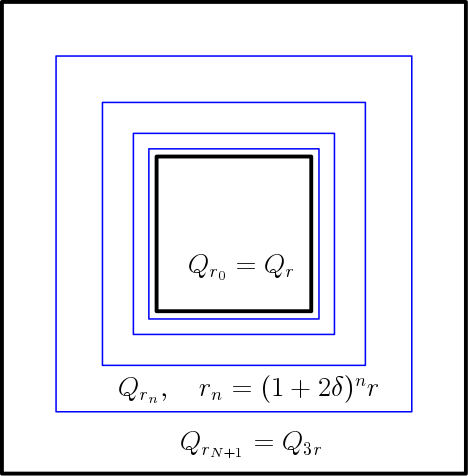
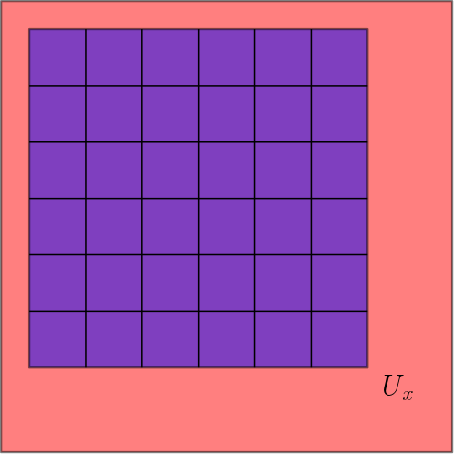
We give the details for this argument—see also Figure 2 for an illustration. We plan to use eq. 3.44 times, and and let , satisfy
| (3.45) |
Then we set the scale and the -harmonic functions in every scale
We can prove by induction that under the condition eq. 3.43. Then for every , we apply eq. 3.44 from on to on
| (3.49) |
Iterating on eq. 3.49 until on , we get
We notice that can be seen as as a weighted sum of , for scales satisfying , by eq. 3.43. So we apply once Jensen’s inequality for and obtain eq. 3.37 by setting
Although we will not use this later, we now give more explicit estimates for the choice of the parameters in the proof above, resulting from the conditions listed in eq. 3.43 and eq. 3.45. It suffices to pick an integer larger than , and then in eq. 3.45 use to fix , and in eq. 3.43 we require , which gives the condition for the minimal scale . A possible choice is the following
4. Subadditive quantities
We aim to adapt the strategy in [11, Chapter 2] for our model in continuum configuration space. In this section, we define several subadditive quantities, denoted by , and develop their elementary properties. We then we use them and a renormalization argument to obtain a quantitative rate of convergence for in Section 5.
4.1. Subadditive quantities and
For every bounded domain and , we define the affine function in with slope by
| (4.1) |
and introduce the subadditive quantities
| (4.2) |
The quantity can be thought of as the average energy per unit volume of the solution which matches with the behavior of the affine function when a particle leaves the domain . The quantity is analogous to a Neumann problem with prescribed average flux of . As will be seen below, the quantities and are approximately dual to one another; the quality of this approximation as the domain grows to will be central to the proof of Theorem 2.1. If the matrix were constant, then by eq. 2.6 the minimizer for would be , and we would have ; and similarly, were constant, we would have .
We start by recording elementary properties satisfied by and . We recall that . For every , we denote by the -enlargement of , that is, .
Proposition 4.1 (Elementary properties of and ).
The following properties hold for every bounded domain with Lipschitz boundary and .
(1) There exists a unique solution for the optimization problem in the definition of that satisfies ; we denote it by . For the optimization problem in the definition of , there exists a maximizer that is -measurable and such that . They are -harmonic functions on , i.e. .
(2) There exist two symmetric matrices and such that
| (4.3) |
and these matrices satisfy and . Moreover,
| (4.4) | ||||
| (4.5) |
(3) Slope: satisfies
| (4.6) |
For the function , there exists a symmetric matrix such that
| (4.7) |
and , so that
| (4.8) |
(4) Quadratic response: for every , we have
| (4.9) |
Similarly, for every , we have
| (4.10) |
(5) The quantities and are subadditive: for every ,
| (4.11) |
Proof.
We prove each of these points in turn.
(1)We study at first the maximizer for the problem . A first observation is that the maximizer can be found in -measurable functions. Because for any , its conditional expectation reaches a larger value for the functional in . We use Jensen’s inequality that
By a variational calculus, we know the characterization of a maximizer with elliptic equation that for any
| (4.12) |
Similarly to the discussion in the proof of Proposition 3.4, we know that a solution for this problem also satisfies the more precise equation
| (4.13) |
and we can define its solution in the space
In this space, we have
by the Poincaré inequality Proposition 3.2. Then the coercivity on left hand side in eq. 4.13 is ensured and we can apply the Lax-Milgram theorem. We call this maximizer . Testing eq. 4.12 with , eq. 2.6 implies that its right hand side is , so we have .
Then we turn to . By a first order variation calculus, we know that a minimizer for is characterized by an elliptic equation that for any
| (4.14) |
We remark that one cannot treat this equation as eq. 4.12, because is not an element in and we cannot subtract it. On the other hand, we can apply the Lax-Milgram theorem on the space
to define the unique solution . We notice that the right hand side of eq. 4.14 is clearly a bounded linear functional, and the coercivity of the left hand side of eq. 4.14 is ensured by the Poincaré inequality Proposition 3.3 on . We denote this minimizer by , and eq. 4.14 implies that .
(2) We test at first eq. 4.14 with and obtain that
| (4.15) |
and this implies is a bilinear map . This definition with eq. 4.15 proves eq. 4.4. We let and obtain that . To obtain the bound of , we use the bound of and the definition of eq. 4.2
We can check that is the minimizer for then it concludes the proof of the bound .
The same argument works for . We test eq. 4.12 with and obtain that
| (4.16) |
This proves that is also bilinear and we denote it by , and this also concludes eq. 4.5. Then we put and eq. 4.16 in the definition of eq. 4.2 that
This proves the bilinear map expression for . Concerning the bound for the matrix , we use the bound for and the equations above to obtain that
| (4.17) |
One can check for the lower bound, attains the maximum and for the upper bound it is that attains the maximum. Then we put the expression and obtain that
which implies the bound for .
(3) The slope identity eq. 4.6 for is directly the result from eq. 2.6 that
For the function , the identity eq. 4.8 comes directly from eq. 4.5, but conditioned , the averaged slope is not . In fact, we recall that is also the conditioned maximizer for eq. 4.13, so we can define the matrix , the quenched slope eq. 4.7. The estimate for this matrix is then obtained by repeating the argument in eq. 4.3 for eq. 4.13.
(4) We test eq. 4.14 with and put it in the left hand side of eq. 4.9
| (4.18) |
The term also appears on the right side of eq. 4.4 with , thus we obtain that
and we put it back to eq. 4.18 to conclude for the validity of eq. 4.9.
Similarly, we develop the left hand side of eq. 4.10 as eq. 4.18, and use eq. 4.12 with to treat the inner product term of and .
We put this term in the left hand side of eq. 4.10 and use the bilinear map expression of to obtain that
This concludes the proof of eq. 4.10.
(5) For , we test the associated variational problem with the candidate , which is an element of , so that
In the last step, we also use the stationarity of the coefficient field .
For , we also use that, for every , we have the inclusion , so its unit energy on every small cube is less than the maximum , thus
4.2. Subadditive quantity
We now study the quantity defined by
| (4.19) |
By the properties of and , the quantity is also subadditive. We briefly explain why this quantity will be convenient for our purposes. If the functions and were exactly convex dual of one another, then we would have that and that for every , the infimum of is zero. This would correspond to the situation in which and are equal, and for every , we would in fact have that . Instead, we will show below that, for any symmetric matrix , we have
The right side of the inequality above can be thought of as a measure of the defect in the convex duality relationship between and . For and using , we obtain that
Since we know that is a decreasing sequence while is a increasing sequence from eq. 4.3 and eq. 4.11, each sequence has a limit. Therefore, once we prove a rate of convergence to zero for , we get that the two limits coincide, and also a rate for the convergence of .
The rest of this section will present this strategy in details. We establish at first a variational description for the quantity and the properties mentioned above.
Lemma 4.2.
(1) For every , we have the variational representation
| (4.20) |
(2) We have that and .
(3) There exists a constant such that and for every symmetric matrix satisfying , we have
| (4.21) |
Proof.
(1) We start by rewriting the expression of using the definition of and the quadratic expression of . Noting also that the maximizer of belongs to , we can write
| (4.22) |
We claim that for any , with , we have
| (4.23) |
To prove it, we can develop the right hand side of eq. 4.23
| (4.24) |
Because , we apply and eq. 2.6, the last line of eq. 4.24 is and we prove eq. 4.23. Then we take the maximum as eq. 4.22 and obtain the definition eq. 4.20.
(2) The properties that comes from the definition of : we test the functional in the definition of with the minimizer of and obtain that
so that
Then we test with that and obtain that
and therefore .
(3) Using this property, we have
We put and obtain . The proof of the statement concerning is similar. ∎
In view of the definition of , this functional enjoys properties similar to those described in Proposition 4.1 for and .
Proposition 4.3 (Elementary properties of ).
For every bounded domain with Lipschitz boundary and , the quantity defined in eq. 4.19 satisfies the following properties:
(1) Characterization of optimizer: the optimization problem in eq. 4.20 admits a unique solution such that . This solution is such that for every ,
| (4.25) |
and a linear map. The function can be expressed in terms of the optimizers in eq. 4.2 as
| (4.26) |
We have the quadratic expression
| (4.27) |
(3) Quadratic response: for every , we have
| (4.29) |
(4) Subadditivity: for every , we have
| (4.30) |
Proof.
(1) The equation eq. 4.25 comes directly from the first order variation calculus. The proof of the existence and uniqueness of the solution is similar as the one for . Equation 4.25 also implies that the map is linear because for any , and any we have
Then is also a solution for the problem eq. 4.25 with parameter . Notice that we have
it implies and the linearity of the map.
The exact expression of comes from the equivalent definition eq. 4.20 of and its proof. We put in the first order variation eq. 4.25
(3) We use the expression in eq. 4.26 with , then we use the quadratic response for eq. 4.10 that
Then we add back the term and it gives the desired result
(4) Equation 4.30 is a consequence of eq. 4.11 and eq. 4.19. ∎
We conclude this section with the following lemma.
Lemma 4.4 (Comparison between two scales).
For every with , and , writing as shorthand for , we have
| (4.31) |
5. Quantitative rate of convergence
We are now ready to prove Theorem 2.1. We decompose the argument into a series of four steps.
5.1. Step 1: setup
We use the shorthand , so that by eq. 4.28, the average slope of the function is , in the sense that
| (5.1) |
We let denote a measure of the defect in the subadditivity of , precisely,
| (5.2) |
A direct corollary from eq. 5.2 is that for any integers ,
| (5.3) |
We recall that is decreasing and is increasing, with the comparison . From eq. 4.21, we know that
From now on, we thus fix , and focus on estimating . We also assume without further notification that is sufficiently large that , for the constant appearing in Proposition 3.9. We use to compare with eq. 4.27 and apply the quadratic response eq. 4.29. In the rest of Step 1, we write as a shorthand for , and decompose
| (5.4) |
with
and
We treat the two terms separately. For eq. 5.4-a, since (see Proposition A.2 for details), we use eq. 4.29 to get
Using Jensen’s inequality, we have
and the conditional expectation also implies that
Thus we combine these terms with the quadratic response eq. 4.29 to obtain
and we use Lemma 4.4 between and to get
| (5.5) |
where the quantity is defined in eq. 5.2.
For the term eq. 5.4-b, we can apply the modified Caccioppoli inequality eq. 3.37: there exist two finite positive constants and such that
| (5.6) |
Using eq. 4.27, we see that the averaged gradient term on the right side of eq. 5.6 is , and eq. 4.30 asserts that . Therefore, we get the bound for eq. 5.4-b
| (5.7) |
We put eq. 5.5 and eq. 5.7 back to eq. 5.4, obtaining
Since , this gives
| (5.8) |
5.2. Step 2: flatness estimate
In this step, we estimate the -flatness of optimizers of . Notice that, using the result of Lemma 5.10 with , the corresponding affine function is and we obtain from eq. 5.8 that
| (5.9) |
Lemma 5.1 (-flatness estimate).
There exist and such that for every and ,
| (5.10) |
Proof.
In the rest of the proof, we write as we will not change in the proof. Since , we can use the multiscale Poincaré inequality eq. 3.23
| (5.11) |
The first term on the right side above is of constant order, by eq. 4.27. For the second term, we use a two-scale comparison for every that
| (5.12) |
For the first term we have
For the second term in eq. 5.12, recalling eq. 3.15, we use Jensen’s inequality and eq. 4.31 to get
For the third term eq. 5.12, we use eq. 3.17, Jensen’s inequality, and stationarity. Here we remark that the operator is a conditional expectation with more information than .
The estimation of this term is postponed to the next step. We will prove in Lemma 5.2 below that
We put these estimates back to eq. 5.11 and obtain that
We square the two sides and use the Cauchy-Schwarz inequality to obtain
as announced. ∎
5.3. Step 3: variance estimate
In this part, we prove the following variance estimate, which was used in Step 2.
Lemma 5.2 (Variance estimate).
There exist and such that for every and ,
| (5.13) |
Proof.
In the rest of the proof, we write , as we will not change in the proof. From eq. 5.1, we know that the average slope of is , and notice that is -measurable. Thus the idea is to use to approximate eq. 5.13 in scale with some error, and then apply the independence for and for large. However, different from the standard elliptic setting, here we will see a renormalization with random weights.
We start by relaxing eq. 5.13 to . We observe that in fact is constant in , so
We denote by the left hand side of eq. 5.13. By triangle inequality, we have
| (5.14) |
with
| eq. 5.14-a | |||
| eq. 5.14-b | |||
| eq. 5.14-c |
For the term eq. 5.14-b, recalling eq. 3.17 and eq. 3.15, we use Jensen’s inequality and the two-scale comparison eq. 4.31 to get
| (5.16) |
The term eq. 5.14-c is the key for our result. To simplify a little more the notation, we write
| (5.17) |
Notice that are -measurable. With this notation in place, we have
and by eq. 5.1,
The term eq. 5.14-c we want to estimate can be rewritten as
| eq. 5.14-c |
If the coefficients were deterministic, then we would be able to leverage on the finite range of dependence of in this variance term. However, since the number of particles is random, we introduce the event
| (5.18) |
thus we can divide eq. 5.14-c into two terms
| eq. 5.14-c | |||
| eq. 5.14-c1 | |||
| eq. 5.14-c2 |
For the term eq. 5.14-c1, we know that is not typical in large scales, and we have the Chernoff bound
Moreover, by the Cauchy-Schwarz inequality,
We need a bound for the term : recalling the definition in eq. 3.15 and eq. 4.28,
Using the martingale structure of eq. 3.17, we have
Then we use Jensen’s inequality and the bound of
| (5.19) |
This concludes that
| (5.20) |
Finally, we treat eq. 5.14-c2. We calculate eq. 5.14-c2 at first with the conditional expectation with respect to . Clearly, is -measurable, and under this condition , so we have
| (5.21) |
We would like to develop the term and also drop out the indicator term. The argument here is deterministic
where . We now add back the indicator and develop it
| (5.22) |
From the first line to the second line above, we use that under the event . We then keep in mind that the quantity in on the second line of eq. 5.22 is always larger than , so it is nonnegative. Therefore, from the second line to the third line, we can drop the indicator function in front. Inserting this estimate into eq. 5.21, we obtain that
The sum in the second line is , because for , and are independent,
For the sum in the first line, is nothing but
We use Jensen’s inequality to shrink the operator to that
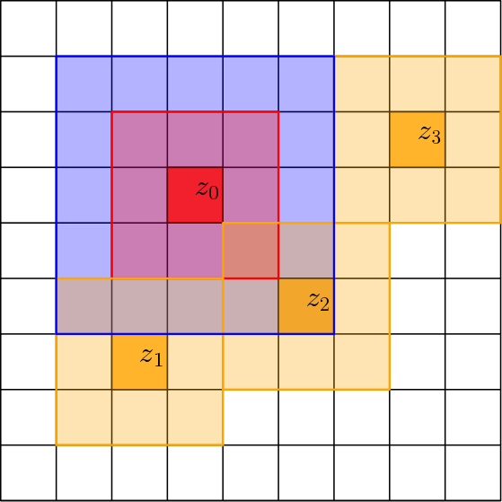
There are at most pairs such that ; see Figure 3 for an illustration. Therefore, we obtain
where we recall that is the left hand side of eq. 5.13. We put this estimate together with eq. 5.15, (5.16), (5.20) back to eq. 5.14 to obtain the recurrence relation
By choosing sufficiently small, we obtain the desired result eq. 5.13. ∎
5.4. Step 4: iterations
Once we obtain the estimate eq. 5.9, it remains to do some numerical iterations, similarly to [11, Page 59-60]. For the reader’s convenience, we recall the main steps here. Let denote the canonical basis in , and define
In order to obtain an exponential decay for , we first introduce a weighted version of this quantity:
Here the exponent is the same as in eq. 5.9. It is clear that , so it suffices to prove an exponential decay for . We will do so by proving a recurrence equation of type for some constant . Thus in the following, we calculate some bounds for and .
Starting with , we write
Noticing that is the minimizer for the mapping in eq. 4.19, we have
| (5.23) |
Using also eq. 4.19, that , and that and are positive semidefinite quadratic forms, we get
and thus
| (5.24) |
For the upper bound of , we use eq. 5.23 to see that , so
Then we apply eq. 5.9 into the result above to get
| (5.25) |
We combine eq. 5.24 and eq. 5.25, to obtain , which implies
for some . We thus conclude for the exponential decay of , and thus also of , since . By eq. 4.21, this completes the proof of Theorem 2.1.
Appendix A Some elementary properties of the function spaces
Lemma A.1 (Canonical projection).
Let be a function, and for every Borel set , measure , and , let denote the (permutation-invariant) function
The following statements are equivalent.
(1) The function is -measurable.
(2) For every , the function is -measurable.
Proof.
We start from . Because , it suffices to study the product function
for some Borel sets . In this case, we have
where is the symmetric group. This proves that is -measurable.
We turn to . Let us pick a suitable and , then the main point is to establish the -measurable property. Since is -measurable and permutation-invariant, it suffices to study the function of type
| (A.1) |
for Borel sets. This is still a complicated function, but we can add one more condition
| (A.2) |
For example, let be all the different elements in , and appears times. For the functions of type eq. A.1 satisfying the condition eq. A.2, the -measurable property is easy to treat since we have
which is an -measurable function.
Proposition A.2.
For every and , we have , and for every
| (A.3) |
Moreover, if and , then .
Proof.
At first, we should remark the well-definedness of the right side of eq. A.3. Notice that the Poisson measure can be decomposed as a sum of the independent parts , we have
Thus the right-hand side of eq. A.3 is defined as
| (A.4) |
We prove eq. A.3 and for the functions in as they are dense, and we can focus on the case fixed. We use Lemma A.1 to write
Following the property of product measure, for every , the mapping
is -measurable. Thus for every , the mapping
is also -measurable because it is the limit of -measurable functions. Then we observe that
as a supremum of a countable number of -measurable functions, is finite and -measurable. Thus we can define a cut-off version of that
and we can establish eq. A.3 at first for . For every , we have
for small enough such that . Since , we use Lemma A.1 and the mean value theorem
for some . With the indicator , this term is bounded by , so we can use the dominated convergence theorem that
which establishes the eq. A.3 in the sense eq. A.4. By Jensen’s inequality and Fubini’s lemma, we observe that
which implies that . Then we use once again Jensen’s inequality for and with
So gives a Cauchy sequence in , and the only candidate is because it is the limit in . By this and a linear combination, we establish eq. A.3 for in , and we can then extend to a general function in by the density argument.
For the part of -harmonic function, we suppose and test with eq. A.3,
Restricted on , we have are -measurable, so we have
We can enter the part in the integration, and then use Fubini’s lemma
In the last step, we use and this finishes the proof. ∎
Appendix B Equivalent definitions of the effective diffusion matrix
Recall that we defined and according to eq. 4.1-eq. 4.3. The proof of Theorem 2.1 ensures the existence of a constant and an exponent such that for every ,
| (B.1) |
Throughout this appendix, we will only rely on the qualitative statement that
| (B.2) |
The first main goal of this appendix is to demonstrate that the definition we chose for the bulk diffusion matrix indeed coincides with the “stationary” definition appearing in works such as [69, 34]. Adapted to our context, this alternative definition takes the following form. For
| (B.3) |
we let be the -by- matrix such that for every ,
| (B.4) |
where in eq. B.3, we used the notation . Notice that for and , the function is typically not well-defined unless is of finite support. However, the quantity makes sense whenever the measure is -finite, since in the sum , the function is local, and thus the integrand is non-zero only for in a bounded set. With this interpretation of , the right side of eq. B.4 is well-defined.
Theorem B.1.
We have .
The second main goal of this appendix is to demonstrate that the infimum in eq. B.4 is achieved in a suitable completion of the space . We also show that the optimizer, which we call the (stationary) corrector, can be obtained as a limit of approximations based on the finite-volume optimizers for or . Denoting
we introduce the space
and its local version
| (B.5) |
In these definitions, we say that is measurable provided that the mapping
is -measurable. The space is naturally endowed with the family of seminorms
indexed by all the compact sets . This family of seminorms turns into a complete space.
For every and , we let be such that the minimizer in the definition of is , where we recall that was defined in eq. 4.1. Similarly, we let be such that is the maximizer in the definition of . More precisely, using the notation introduced in Proposition 4.1, we have
and
Finally, we define according to the formula
| (B.6) |
Notice that, while is ill-defined when , the quantity is still well-defined, for the same reason as in the discussion following eq. B.4. Our second main result is as follows.
Theorem B.2.
The following statements hold for every .
(1) The sequence is a Cauchy sequence in . Its limit, which we denote by , satisfies
| (B.7) |
(2) We have
| (B.8) |
as well as
| (B.9) |
(3) The effective diffusion matrix satisfies
| (B.10) |
as well as
| (B.11) |
As a preparation towards the proof of these results, we state in the following proposition a number of elementary properties about the function space .
Proposition B.3.
Let be an -measurable function, and let . The following properties hold:
- (1)
is a stationary field, i.e. .
- (2)
has mean zero, that is,
(B.12) - (3)
satisfies the estimate
(B.13)
Proof.
(1) We use the definition to write
From the first line to the second line, we used the fact that is -measurable, so if the transport vector does not belong to , then the integrand vanishes (up to a boundary layer that vanishes in the limit ). We then do the change of variables to get
which means that is a stationary gradient field.
(2) We use the equations developed in the last question. Since , we can exchange the integration and derivative and get
| (B.14) |
We evaluate this gradient at
From the second line to the third line, we used the stationarity of the Poisson point process. Because , then and the integration in the third line vanishes.
(3) We pick a cube with , make use of the stationarity of and Mecke’s identity (see [52, Theorem 4.1])
We put the definition into the equation. For the gradient at , as is -measurable, thus only the term for contributes. This gives
We next apply Jensen’s inequality to obtain that
| (B.15) |
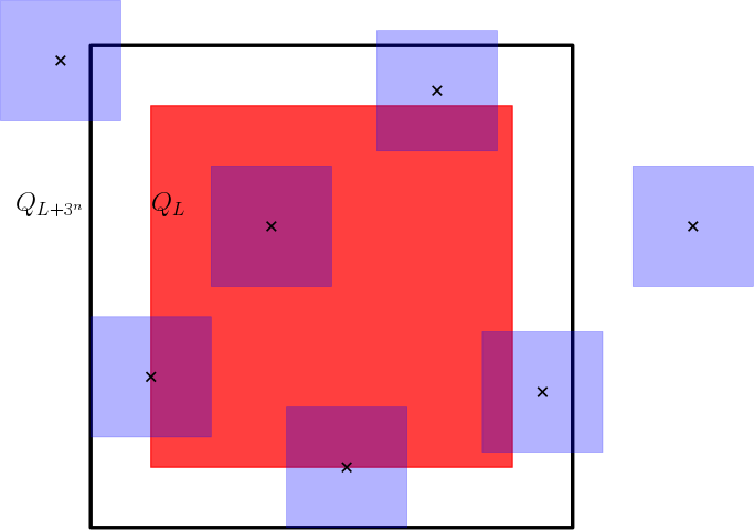
In the last line, we use Fubini’s lemma and exchange with . In this procedure, we have to enlarge the domain from to , because for the gradient at , contributes for the transport (see Figure 4 as an illustration). Using the stationarity of the Poisson point process, we have
which helps us conclude that
We take and obtain the desired result. ∎
Remark B.4.
The inequality eq. B.13 is essentially sharp when itself is close to a stationary field. Indeed, if is close to a stationary field, then
which implies that the application of Jensen’s inequality in eq. B.15 is essentially sharp. The error introduced by a boundary layer in a subsequent step of the proof disappears as we take at the end.
As a corollary of Proposition B.3, we can also propose the following equivalent definition of .
Corollary B.5.
For any open set , we have
| (B.16) |
Proof.
It is a direct result of Mecke’s identity (see [52, Theorem 4.1]) and the stationarity of . ∎
With the help of Proposition B.3, we can now prove the first main theorem of this appendix.
Proof of Theorem B.1.
We decompose the proof into two steps.
Step 1: Bound from below . We fix and a sequence of approximate minimizers for the variational problem in eq. B.4, which we write in the form
for some . Now we propose a modified version in defined by
with a large compact set so that and
Then we test in the optimization problem for to get that
We use the stationarity of , eq. B.12 and let to obtain
Taking leads to
Finally, we let and conclude that .
Step 2: Bound from above . We hope to prove by testing the variational formula eq. B.4 with a suitable candidate, namely the function introduced in eq. B.6. Since , and using eq. B.13, we can approximate in arbitrarily closely with elements of . It thus follows that we can use as a candidate in the variational problem in eq. B.4, and use the comparison inequality eq. B.13 to get that
| (B.17) | ||||
Finally, we let and conclude that . ∎
In the proof above, we used as a sequence of approximate minimizers for the variational problem in eq. B.4. This already gives us a good hint for the validity of at least some of the statements in Theorem B.2. We now turn to the proof of the first part of this result.
Proof of part (1) of Theorem B.2.
We decompose the proof into four steps.
Step 1: is a Cauchy sequence in . We fix and, recalling the notation , we observe that
where the function is defined as
| (B.18) |
For any compact set , we use Mecke’s identity (see [52, Theorem 4.1]) and the stationarity of
Then we use the comparison inequality eq. B.13 and obtain that
By eq. B.2, this shows that is a Cauchy sequence in .
Step 2: Harmonic property - setting up. Denote the limit by , we set things up to prove the harmonic property eq. B.7 by approximation. We fix and which is -measurable, and observe that
We then use Fubini’s lemma to exchange the order of integration,
For sufficiently large, we can decompose the domain of integration in in the expression above into and . We analyse the contribution of each of these quantities in each of the following two steps.
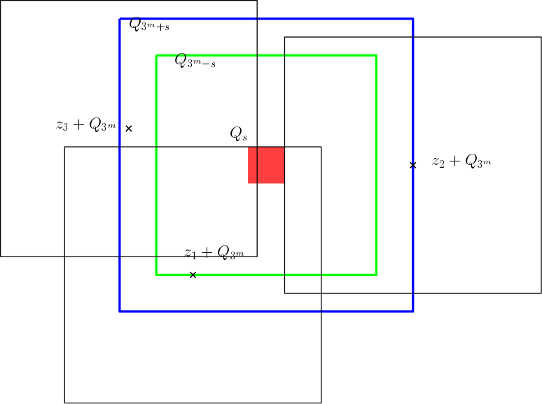
Step 3: Integration in . Notice that for , we have (see Figure 5 for an illustration), thus we can drop the indicator in the inner integral and use the -harmonic property of to get that
Step 4: Boundary layer . We use Young’s inequality to bound the term with the integral over by
For the term , we have, for a constant that may depend on ,
For the term , we use the stationarity to observe that
We apply once again Fubini’s lemma to and get that
That this term converges to zero is a consequence of the stronger estimate given by Lemma B.6 below. This concludes the proof for , and then we can use density argument to extend to general . ∎
In the proof above, we appealed to the following boundary layer estimate, which we state as a separate lemma for future reference (and which is stronger than what was needed for the purpose of the proof above, since the boundary layer size is allowed to increase with ).
Lemma B.6 (Boundary layer estimate).
For every sequence such that and , we have
| (B.19) |
Proof.
The idea is to make use of the renormalization argument. We define a mesoscopic scale associated to such that , and . Then we immediately have
We propose to compare with defined as in eq. B.18:
Then we have
| (B.20) |
For the first term eq. B.20-a, we do partition of sum into cubes of size , then we have
For the second term eq. B.20-b, we have
Therefore, when we take , both eq. B.20-a and eq. B.20-b go to , so the boundary layer in a mecroscopic scale can be neglected. ∎
Now that the gradient of the whole-space corrector is well-defined, we can proceed to complete the proof of Theorem B.2.
Proof of parts (2) and (3) of Theorem B.2.
We start by discussing the validity of the identities eq. B.10 and eq. B.11. We use the stationary approximate corrector defined in eq. B.6, and observe from eq. B.17 and Theorem B.1 that
The identity eq. B.10 then follows from the convergence of to in . For the second identity, we can use the fact that
the estimate eq. B.8, and the stationarity of . The identity eq. B.9 can also be deduced from eq. B.8 because
By eq. 4.26 and eq. 4.27, the second term can be bounded by ; and by eq. 4.19 and eq. B.2, this quantity converges to as . From now on, we thus focus on the proof of eq. B.8.
The idea of the proof of eq. B.8 is very close to that for eq. B.7 and eq. B.19. We fix a mescroscopic scale , and then use the decomposition
| (B.21) |
For the first term eq. B.21-a, we use the stationarity to transform to the integration on unit cube , and then use the fact that converges to in to get that
Thus it suffices to finish the second term eq. B.21-b. We use the definition in eq. B.6 and Jensen’s inequality to get that
| eq. B.21-b | |||
where in the last line we decompose once again the integration into three terms with respect to the domain
| eq. B.21-b1 | |||
| eq. B.21-b2 | |||
| eq. B.21-b3 |
The terms eq. B.21-b2 and eq. B.21-b3 are easy to treat as they are boundary layer terms. For eq. B.21-b2 we can use the energy bound
For eq. B.21-b3, since the function does not involve , we use Fubini’s lemma that
| eq. B.21-b3 | |||
Here from the second line to the third line, we use the fact that the gradient contributes only on . Then we do a decomposition: the integration on can be calculated directly, since is -measurable and the gradient vanishes; the integration on can be bounded by the boundary layer estimate in Lemma B.6.
Finally, we focus on eq. B.21-b1. We rewrite the integration as
For each fixed , we can propose a sub-minimizer for defined by (see Figure 6 for an illustration)
where
The gradient of and coincides on every cube , so we can write
where we used the quadratic response (4.9) from the second line to the third line. This implies that , and thus completes the proof of eq. B.8. ∎
Acknowledgements
Part of this project was developed while AG was affiliated to the University of Bonn and supported through the CRC 1060 (The Mathematics of Emergent Effects) that is funded through the German Science Foundation (DFG), and the Hausdorff Center for Mathematics (HCM). CG was supported by a PhD scholarship from Ecole Polytechnique. Part of this project was developed while CG was an academic visitor at the Courant Institute, NYU. JCM was partially supported by the NSF grant DMS-1954357. Part of this project was developed while JCM was affiliated at CNRS and ENS Paris, PSL University, and was partially supported by the ANR grants LSD (ANR-15-CE40-0020-03) and Malin (ANR-16-CE93-0003).
References
- [1] S. Albeverio, Y. G. Kondratiev, and M. Röckner. Canonical Dirichlet operator and distorted Brownian motion on Poisson spaces. C. R. Acad. Sci. Paris Sér. I Math., 323(11):1179–1184, 1996.
- [2] S. Albeverio, Y. G. Kondratiev, and M. Röckner. Differential geometry of Poisson spaces. C. R. Acad. Sci. Paris Sér. I Math., 323(10):1129–1134, 1996.
- [3] S. Albeverio, Y. G. Kondratiev, and M. Röckner. Analysis and geometry on configuration spaces. J. Funct. Anal., 154(2):444–500, 1998.
- [4] S. Albeverio, Y. G. Kondratiev, and M. Röckner. Analysis and geometry on configuration spaces: the Gibbsian case. J. Funct. Anal., 157(1):242–291, 1998.
- [5] S. Armstrong, A. Bordas, and J.-C. Mourrat. Quantitative stochastic homogenization and regularity theory of parabolic equations. Analysis & PDE, 11(8):1945–2014, 2018.
- [6] S. Armstrong and P. Dario. Elliptic regularity and quantitative homogenization on percolation clusters. Commun. Pure Appl. Math., 71(9):1717–1849, 2018.
- [7] S. Armstrong, S. Ferguson, and T. Kuusi. Homogenization, linearization and large-scale regularity for nonlinear elliptic equations. Comm. Pure Appl. Math., to appear.
- [8] S. Armstrong, S. J. Ferguson, and T. Kuusi. Higher-order linearization and regularity in nonlinear homogenization. Arch. Ration. Mech. Anal., 237(2):631–741, 2020.
- [9] S. Armstrong, T. Kuusi, and J.-C. Mourrat. Mesoscopic higher regularity and subadditivity in elliptic homogenization. Comm. Math. Phys., 347(2):315–361, 2016.
- [10] S. Armstrong, T. Kuusi, and J.-C. Mourrat. The additive structure of elliptic homogenization. Invent. Math., 208(3):999–1154, 2017.
- [11] S. Armstrong, T. Kuusi, and J.-C. Mourrat. Quantitative stochastic homogenization and large-scale regularity, volume 352 of Grundlehren der mathematischen Wissenschaften. Springer Nature, 2019.
- [12] S. Armstrong and W. Wu. regularity of the surface tension for the interface model. Preprint, arXiv:1909.13325.
- [13] S. N. Armstrong and J.-C. Mourrat. Lipschitz regularity for elliptic equations with random coefficients. Arch. Ration. Mech. Anal., 219(1):255–348, 2016.
- [14] S. N. Armstrong and C. K. Smart. Quantitative stochastic homogenization of convex integral functionals. Ann. Sci. Éc. Norm. Supér. (4), 49(2):423–481, 2016.
- [15] C. Bernardin. Regularity of the diffusion coefficient for lattice gas reversible under Bernoulli measures. Stochastic Process. Appl., 101(1):43–68, 2002.
- [16] L. Bertini and B. Zegarlinski. Coercive inequalities for Kawasaki dynamics. The product case. Markov Process. Related Fields, 5(2):125–162, 1999.
- [17] T. Bodineau, I. Gallagher, L. Saint-Raymond, and S. Simonella. Statistical dynamics of a hard sphere gas: fluctuating Boltzmann equation and large deviations. Preprint, arXiv:2008.10403.
- [18] T. Brox and H. Rost. Equilibrium fluctuations of stochastic particle systems: the role of conserved quantities. Ann. Probab., 12(3):742–759, 1984.
- [19] N. Cancrini, F. Cesi, and C. Roberto. Diffusive long-time behavior of Kawasaki dynamics. Electron. J. Probab., 10:no. 7, 216–249, 2005.
- [20] C. C. Chang. Equilibrium fluctuations of gradient reversible particle systems. Probab. Theory Related Fields, 100(3):269–283, 1994.
- [21] C.-C. Chang. Equilibrium fluctuations of nongradient reversible particle systems. In Nonlinear stochastic PDEs (Minneapolis, MN, 1994), volume 77 of IMA Vol. Math. Appl., pages 41–51. Springer, New York, 1996.
- [22] C. C. Chang and H.-T. Yau. Fluctuations of one-dimensional Ginzburg-Landau models in nonequilibrium. Comm. Math. Phys., 145(2):209–234, 1992.
- [23] P. Dario. Quantitative homogenization of the disordered model. Electron. J. Probab., 24:Paper No. 90, 99p., 2019.
- [24] P. Dario. Optimal corrector estimates on percolation cluster. Ann. Appl. Probab., 31(1):377–431, 2021.
- [25] P. Dario. Quantitative homogenization of differential forms. Ann. Inst. Henri Poincaré Probab. Stat., 57(2):1157–1202, 2021.
- [26] P. Dario and C. Gu. Quantitative homogenization of the parabolic and elliptic Green’s functions on percolation clusters. Ann. Probab., 49(2):556–636, 2021.
- [27] P. Dario and W. Wu. Massless phases for the Villain model in . Preprint, arXiv:2002.02946.
- [28] A. De Masi, P. A. Ferrari, and J. L. Lebowitz. Reaction-diffusion equations for interacting particle systems. J. Statist. Phys., 44(3-4):589–644, 1986.
- [29] A. De Masi, E. Presutti, H. Spohn, and W. D. Wick. Asymptotic equivalence of fluctuation fields for reversible exclusion processes with speed change. Ann. Probab., 14(2):409–423, 1986.
- [30] J.-D. Deuschel. Algebraic decay of attractive critical processes on the lattice. Ann. Probab., 22(1):264–283, 1994.
- [31] M. Duerinckx and A. Gloria. Analyticity of homogenized coefficients under Bernoulli perturbations and the Clausius-Mossotti formulas. Arch. Ration. Mech. Anal., 220(1):297–361, 2016.
- [32] P. A. Ferrari, E. Presutti, and M. E. Vares. Nonequilibrium fluctuations for a zero range process. Ann. Inst. H. Poincaré Probab. Statist., 24(2):237–268, 1988.
- [33] T. Funaki. Equilibrium fluctuations for lattice gas. In Itô’s stochastic calculus and probability theory, pages 63–72. Springer, Tokyo, 1996.
- [34] T. Funaki, K. Uchiyama, and H. T. Yau. Hydrodynamic limit for lattice gas reversible under Bernoulli measures. In Nonlinear stochastic PDEs (Minneapolis, MN, 1994), volume 77 of IMA Vol. Math. Appl., pages 1–40. Springer, New York, 1996.
- [35] A. Giunti, Y. Gu, and J.-C. Mourrat. Heat kernel upper bounds for interacting particle systems. Ann. Probab., 47(2):1056–1095, 2019.
- [36] A. Gloria, S. Neukamm, and F. Otto. Quantification of ergodicity in stochastic homogenization: optimal bounds via spectral gap on Glauber dynamics. Invent. Math., 199(2):455–515, 2015.
- [37] A. Gloria, S. Neukamm, and F. Otto. A regularity theory for random elliptic operators. Milan J. Math., 88(1):99–170, 2020.
- [38] A. Gloria and F. Otto. An optimal variance estimate in stochastic homogenization of discrete elliptic equations. Ann. Probab., 39(3):779–856, 2011.
- [39] A. Gloria and F. Otto. An optimal error estimate in stochastic homogenization of discrete elliptic equations. Ann. Appl. Probab., 22(1):1–28, 2012.
- [40] A. Gloria and F. Otto. Quantitative results on the corrector equation in stochastic homogenization. J. Eur. Math. Soc. (JEMS), 19(11):3489–3548, 2017.
- [41] C. Gu. Decay of semigroup for an infinite interacting particle system on continuum configuration spaces. Preprint, arXiv:2007.04058.
- [42] M. Z. Guo, G. C. Papanicolaou, and S. R. S. Varadhan. Nonlinear diffusion limit for a system with nearest neighbor interactions. Comm. Math. Phys., 118(1):31–59, 1988.
- [43] E. Janvresse, C. Landim, J. Quastel, and H. T. Yau. Relaxation to equilibrium of conservative dynamics. I. Zero-range processes. Ann. Probab., 27(1):325–360, 1999.
- [44] M. Jara. Finite-dimensional approximation for the diffusion coefficient in the simple exclusion process. Ann. Probab., 34(6):2365–2381, 2006.
- [45] M. Jara and O. Menezes. Non-equilibrium fluctuations of interacting particle systems. Preprint, arXiv:1810.09526.
- [46] C. Kipnis and C. Landim. Scaling limits of interacting particle systems, volume 320 of Grundlehren der Mathematischen Wissenschaften. Springer-Verlag, Berlin, 1999.
- [47] T. Komorowski, C. Landim, and S. Olla. Fluctuations in Markov processes, volume 345 of Grundlehren der Mathematischen Wissenschaften. Springer, Heidelberg, 2012.
- [48] C. Landim, S. Olla, and S. R. S. Varadhan. Symmetric simple exclusion process: regularity of the self-diffusion coefficient. Comm. Math. Phys., 224(1):307–321, 2001. Dedicated to Joel L. Lebowitz.
- [49] C. Landim, S. Olla, and S. R. S. Varadhan. Finite-dimensional approximation of the self-diffusion coefficient for the exclusion process. Ann. Probab., 30(2):483–508, 2002.
- [50] C. Landim, S. Olla, and S. R. S. Varadhan. On viscosity and fluctuation-dissipation in exclusion processes. J. Statist. Phys., 115(1-2):323–363, 2004.
- [51] C. Landim and H. T. Yau. Convergence to equilibrium of conservative particle systems on . Ann. Probab., 31(1):115–147, 2003.
- [52] G. Last and M. Penrose. Lectures on the Poisson process, volume 7 of Institute of Mathematical Statistics Textbooks. Cambridge University Press, Cambridge, 2018.
- [53] G. Leoni. A first course in Sobolev spaces, volume 181 of Graduate Studies in Mathematics. American Mathematical Society, Providence, RI, second edition, 2017.
- [54] T. M. Liggett. rates of convergence for attractive reversible nearest particle systems: the critical case. Ann. Probab., 19(3):935–959, 1991.
- [55] S. L. Lu. Equilibrium fluctuations of a one-dimensional nongradient Ginzburg-Landau model. Ann. Probab., 22(3):1252–1272, 1994.
- [56] J.-C. Mourrat. Variance decay for functionals of the environment viewed by the particle. Ann. Inst. Henri Poincaré Probab. Stat., 47(1):294–327, 2011.
- [57] J.-C. Mourrat. First-order expansion of homogenized coefficients under Bernoulli perturbations. J. Math. Pures Appl. (9), 103(1):68–101, 2015.
- [58] J.-C. Mourrat. An informal introduction to quantitative stochastic homogenization. J. Math. Phys., 60(3):031506, 11, 2019.
- [59] A. Naddaf and T. Spencer. Estimates on the variance of some homogenization problems, 1998, unpublished preprint.
- [60] Y. Nagahata. Regularity of the diffusion coefficient matrix for the lattice gas with energy. Ann. Inst. H. Poincaré Probab. Statist., 41(1):45–67, 2005.
- [61] Y. Nagahata. Regularity of the diffusion coefficient matrix for generalized exclusion process. Stochastic Process. Appl., 116(6):957–982, 2006.
- [62] Y. Nagahata. Regularity of the diffusion coefficient matrix for lattice gas reversible under Gibbs measures with mixing condition. Comm. Math. Phys., 273(3):637–650, 2007.
- [63] E. Presutti and H. Spohn. Hydrodynamics of the voter model. Ann. Probab., 11(4):867–875, 1983.
- [64] J. Quastel. Diffusion of color in the simple exclusion process. Comm. Pure Appl. Math., 45(6):623–679, 1992.
- [65] M. Röckner. Stochastic analysis on configuration spaces: basic ideas and recent results. In New directions in Dirichlet forms, volume 8 of AMS/IP Stud. Adv. Math., pages 157–231. Amer. Math. Soc., Providence, RI, 1998.
- [66] H. Spohn. Equilibrium fluctuations for interacting Brownian particles. Comm. Math. Phys., 103(1):1–33, 1986.
- [67] H. Spohn. Large scale dynamics of interacting particles. Texts and Monographs in Physics. Springer-Verlag, Berlin, 1991.
- [68] M. Sued. Regularity properties of the diffusion coefficient for a mean zero exclusion process. Ann. Inst. H. Poincaré Probab. Statist., 41(1):1–33, 2005.
- [69] S. R. S. Varadhan. Nonlinear diffusion limit for a system with nearest neighbor interactions. II. In Asymptotic problems in probability theory: stochastic models and diffusions on fractals (Sanda/Kyoto, 1990), volume 283 of Pitman Res. Notes Math. Ser., pages 75–128. Longman Sci. Tech., Harlow, 1993.
- [70] S. R. S. Varadhan. Regularity of self-diffusion coefficient. In The Dynkin Festschrift, volume 34 of Progr. Probab., pages 387–397. Birkhäuser Boston, Boston, MA, 1994.
- [71] H.-T. Yau. Relative entropy and hydrodynamics of Ginzburg-Landau models. Lett. Math. Phys., 22(1):63–80, 1991.