跳到论文正文
W Papers独立论文阅读器 arXiv:2011.06327 论文正文 计算阅读时间 · 0%
引用这篇论文根据当前论文元数据生成,正式投稿前建议核对。


License: arXiv.org perpetual non-exclusive license
arXiv:2011.06327v4 [math.OC] 06 Jul 2022

Near-Optimal Primal-Dual Algorithms for Quantity-Based Network Revenue Management

Rui Sun    Xinshang Wang    Zijie Zhou
Abstract

We study the canonical quantity-based network revenue management (NRM) problem where the decision-maker must irrevocably accept or reject each arriving customer request with the goal of maximizing the total revenue given limited resources. The exact solution to the problem by dynamic programming is computationally intractable due to the well-known curse of dimensionality. Existing works in the literature make use of the solution to the deterministic linear program (DLP) to design asymptotically optimal algorithms. Those algorithms rely on repeatedly solving DLPs to achieve near-optimal regret bounds. It is, however, time-consuming to repeatedly compute the DLP solutions in real time, especially in large-scale problems.

In this paper, we propose innovative algorithms for the NRM problem that are easy to implement and do not require solving any DLPs. Our algorithm achieves a regret bound of o⁡(T)o(\sqrt{T}), where TT is the system size. To the best of our knowledge, this is the first NRM algorithm that (i) has an o⁡(T)o(\sqrt{T}) asymptotic regret bound, and (ii) does not require solving any DLPs.

††runningauthor: Sun, Wang, and Zhou††runningtitle: Near-Optimal Primal-Dual Algorithms for NRM††authors: Alibaba Group US, Bellevue, WA, 98004, sunruimit@gmail.com Alibaba Group US, Bellevue, WA, 98004, xinshang.w@alibaba-inc.com Operations Research Center, Massachusetts Institute of Technology, Cambridge, MA, 02139, zhou98@mit.edu ††affiliation: ††affiliation: ††affiliation: ††affiliation: ††affiliation: ††affiliation:

1 Introduction

In this paper, we consider the canonical network revenue management (NRM) problem (Williamson 1992, Talluri and Van Ryzin 1998), which finds applications in airline, retail, advertising, and hospitality (Talluri and Van Ryzin 2004). The NRM problem is stated as follows: there is a set of resources with limited capacities that are available over a finite time horizon. Customers of different types arrive sequentially over time. The type of a customer is defined by the customer’s consumption of resources and the price she pays. Each type of customer requests a certain amount of each resource. Upon a customer’s arrival, the decision-maker needs to decide whether to accept or reject the customer. Accepting the customer generates a certain amount of revenue, which equals the price the customer pays, and also consumes certain units of each resource associated with the customer’s type. Rejecting the customer generates no revenue and uses no resources. The objective is to maximize the total expected revenue during the entire horizon under the capacity constraints of all the resources.

The model we focus on in this paper is known as the “quantity-based” NRM model. There exists another well-known NRM model called the “price-based” model. In the price-based NRM problem, the decision-maker chooses product prices rather than admission (accept/reject) decisions. These two models are different but are equivalent in certain special cases, such as the single resource multi-product model suggested in Maglaras and Meissner 2006.

A classic example of the NRM problem is airline seat allocation. In this problem, resources correspond to flight legs and the capacity of a resource corresponds to the number of seats on the flight. Each customer requests a flight itinerary that consists of a single or multiple flight legs (thus a network structure) and pays the ticket price of the itinerary. Arriving customers are sorted into different classes based on combinations of itinerary and price. This allows the airline to maximize the expected revenue by allocating seats on different flights to different customer classes.

In theory, the NRM problem can be solved by dynamic programming. The state is described jointly by time and the remaining capacities of all the resources. The optimal admission policy compares the revenue of each arriving customer with the marginal value of the requested resources and accepts the customer if the former is larger. However, the time complexity of this optimal algorithm grows exponentially with the number of resources, and is thus computationally intractable. In this paper, we study approximate algorithms that are easy to implement and have provable performance guarantees.

One of the most used mathematical tools for designing and analyzing approximate algorithms in the NRM literature is the deterministic linear program (DLP) formulation. See Section 1.2 for a detailed review of algorithms based on solutions of the DLP. Typically, the DLP is formulated by replacing random variables in the model with their distributional information (e.g., replacing random demand variables with their expectations).

The DLP formulation is essential in the following two aspects. First, an optimal solution to the DLP is a guideline for making online decisions. Specifically, the primal solution of the DLP can be used to design booking limit heuristics, nesting strategies (Talluri and Van Ryzin 2004), and probabilistic assignment policies (Reiman and Wang 2008, Jasin and Kumar 2012, Bumpensanti and Wang 2020). In addition, the dual solution of the DLP serve as bid prices in bid-price control heuristics (Talluri and Van Ryzin 1998). Second, the DLP provides an upper bound on the optimal revenue since the capacity constraints in the DLP are only satisfied in expectation. The DLP upper bound (and its variants) is considered the benchmark performance in the analysis of many algorithms.

In the literature of quantity-based NRM, Reiman and Wang 2008, Jasin and Kumar 2012, and Bumpensanti and Wang 2020 show much better regret bounds compared to preceding results by (re-)solving DLPs multiple times. More precisely, Reiman and Wang 2008 show that strategically resolving the DLP once achieves a regret bound of o⁡(T)o(\sqrt{T}), where T=1,2​…T=1,2\ldots is the system size, improving upon the classic O⁡(T)O(\sqrt{T}) bounds (Talluri and Van Ryzin 2004). Jasin and Kumar 2012 show that resolving the DLP in every time period achieves a regret bound of O⁡(1)O(1). Bumpensanti and Wang 2020 prove a uniform regret bound of O⁡(1)O(1) that does not depend on any numerical values in the solutions of the DLP.

Despite the theoretical developments for the NRM problem, there are challenges in implementing those algorithms that require solving DLPs in an online manner. First, direct linear system solvers, which are necessary for solving DLPs, are time consuming for large-scale problems. Second, consider e-commerce platforms that must deal with more than hundreds of customer visits per second 11 1 For example, 62 million monthly visits took place on Expedia in 2018 (Medium 2018), and 193 million bookings on Airbnb in 2020 (Airbnb 2020). In a typical implementation of online algorithms on such e-commerce platforms, DLPs are solved on dedicated computational servers, which sync with an online streaming database at a much lower rate. In such cases, algorithms handling the online customer traffic are not able to acquire DLP solutions to real-time models.

To overcome these difficulties, we propose primal-dual algorithms that are amenable to online platforms. Our algorithm does not require solving any linear programs or performing any matrix factorization, and still achieves an o⁡(T)o(\sqrt{T}) regret bound.

Similar motivations for such fast online algorithms that do not require solving any linear programs are also considered in Li et al. 2020. Specifically, Li et al. 2020 study the online linear programming model, which is a generalization of the quantity-based NRM model studied in this paper. We show that our algorithm achieves a regret bound of o⁡(T)o(\sqrt{T}), while the algorithm in Li et al. 2020 for the generalized problem achieves a regret bound of O⁡(T)O(\sqrt{T}). We will discuss more differences between our work and Li et al. 2020 in Section 1.2.

1.1 Overview of main results

Table 1 summarizes the related regret bounds proved in the literature, and our results in this paper. In the table, TT stands for the scaling factor, namely the size of the system.

The algorithms proposed in Reiman and Wang 2008, Jasin and Kumar 2012, Bumpensanti and Wang 2020 are re-solving algorithms for the NRM problem. The regret bound proved in Reiman and Wang 2008 grows slower than O⁡(T)O(\sqrt{T}), and the regret bounds proved in Jasin and Kumar 2012, Bumpensanti and Wang 2020 are O⁡(1)O(1). The main intuition behind their algorithms is as follows: if the algorithm makes a mistake of accepting too many customers of a certain type in an earlier stage, then after re-solving the DLP, the algorithm is able to correct the mistake by accepting fewer customers of that type in later periods. Li and Ye 2019 also prove an o⁡(T)o(\sqrt{T}) regret bound but for a more general online linear programming model. All those algorithms that obtain o⁡(T)o(\sqrt{T}) regret bounds require solving the DLP at least twice. In particular, at least one of the DLPs has to be solved online. That is, the algorithms need to wait for the DLP solution before making any further online decisions.

In this paper, we propose three two algorithms that do not require solving any DLPs for the NRM problem. Both algorithms are based on primal-dual frameworks, and they apply online convex optimization (Hazan 2019) techniques to learn the optimal dual values (or bid prices) of the resources. We introduce our first algorithm (Algorithm 2) in Section 3. We show that Algorithm 2 has a regret bound of O⁡(T)O(\sqrt{T}). This algorithm is a warm up for our subsequent main results. It can also be viewed as a direct adaptation of the existing algorithms, such as Li and Ye 2019, Li et al. 2020, Balseiro et al. 2020a, Balseiro et al. 2020b, Agrawal and Devanur 2014 and Agrawal and Devanur 2016.

In Section 4, we introduce a new algorithm (Algorithm 3). It builds on Algorithm 2 and uses a “thresholding” technique for making admission decisions. The algorithms in Bumpensanti and Wang 2020 use a similar thresholding technique. Their algorithm relies on repeatedly solving DLPs to calculate the threshold values. By contrast, in our algorithm, the threshold values are adaptively computed based on a novel statistical property of the admission decisions. We show that Algorithm 3 has a regret bound of O⁡(T3/8​(log⁡T)54)O(T^{3/8}(\log T)^{\frac{5}{4}}). To the best of our knowledge, Algorithm 3 is the first algorithm, for any dynamic multi-resource allocation problem, that (i) has an o⁡(T)o(\sqrt{T}) asymptotic regret bound and (ii) does not require solving any DLPs (or equivalently time-consuming problems).

In Section 5, we provide results from numerical experiments to demonstrate the performance of all these algorithms.

Table 1: List of regret bounds for models applicable to NRM
Previous work Arrival assumptions Regret bound Number of times solving LPs
Reiman and Wang 2008 known i.i.d. o⁡(T)o(\sqrt{T}) 22
Jasin and Kumar 2012 known i.i.d. O⁡(1)O(1) Θ⁡(T)\Theta(T)
Bumpensanti and Wang 2020 known i.i.d. O⁡(1)O(1) Θ⁡(log⁡log⁡T)\Theta(\log\log T)
Agrawal and Devanur 2014 unknown i.i.d. O⁡(T)O(\sqrt{T}) 1
Li and Ye 2019 unknown i.i.d. O⁡(T)O(\sqrt{T}) Θ⁡(log⁡T)\Theta(\log T)
Li and Ye 2019 unknown i.i.d. O⁡(log⁡T​log⁡log​T)O(\log T\log\log T) Θ⁡(T)\Theta(T)
Li et al. 2020 unknown i.i.d. & random permutation O⁡(T)O(\sqrt{T}) 00
Balseiro et al. 2020a, Balseiro et al. 2020b unknown i.i.d. O⁡(T)O(\sqrt{T}) 00
Our algorithms Regret bound Number of times solving LPs
Algorithm 2 O⁡(T)O(\sqrt{T}) 00
Algorithm 3 o⁡(T)o(\sqrt{T}) 00

1.2 Other related work

We study in this paper a canonical network revenue management problem that has a quantity-based formulation. Compared with a price-based formulation as studied in Gallego and Van Ryzin 1994, Gallego and Van Ryzin 1997, both formulations can be solved using dynamic programming (DP). However, the curse of dimensionality renders the DP computationally intractable even for moderate size problems. Therefore, this has motivated studies in the literature to find approximate algorithms for both formulations.

In the price-based formulation, the decision-maker chooses posted prices of different products. In this stream of literature, Gallego and Van Ryzin 1997 show that a static fixed-price policy is asymptotically optimal on the fluid scale (see the definitions of fluid scale optimality and diffusion scale optimality in Section 2.1). It achieves a regret bound of O⁡(T)O(\sqrt{T}) given system size TT. Maglaras and Meissner 2006 and Chen and Farias 2013 study the potential benefit of re-optimization to improve the static control policy. Jasin and Kumar 2012 and Atar and Reiman 2013 propose policies that are optimal on the diffusion scale.

For the quantity-based formulation, a review of DLP-based algorithms can be found in the book by Talluri and Van Ryzin 2004. Here, we briefly review a few commonly used control policies: booking limit control, nesting and bid-price control.

Booking limit control sets a fixed quota for each customer type and accepts customers in a first-come-first-serve (FCFS) fashion. The booking limits are given by DLP solutions, as proposed in Williamson 1992. Later, many variants of the DLP are proposed, e.g., Wollmer 1992 and Li and Yao 2004, to improve the practical performance of the booking limit control policy.

Nesting is a remedy strategy for booking limit control. The nesting policy ranks different customer types based on their revenue and resource usage, and allows high-ranking types to use the quota of the low-ranking types. The nesting policy is shown to be effective for single-resource problems. However, when there exist multiple resources, Talluri and Van Ryzin 1998 show that the advantage of nesting is less clear due to the ambiguity in ranking different customer types.

Bid-price control uses dual variables of DLPs to decide admissions. Bid prices are defined as the Lagrangian multipliers associated with the capacity constraints. A customer is accepted if the price she pays is higher than the estimated value of the requested resource. Talluri and Van Ryzin 1998 provide a comprehensive analysis on the asymptotic optimality of bid-price control, and a comparison of different methods to estimate bid prices.

The quantity-based NRM model in this paper is also related to the online knapsack/secretary problems in Arlotto and Xie 2018 and Arlotto and Gurvich 2019, the packing/matching problems in Vera and Banerjee 2020, and the online linear programming (OLP) problems in Agrawal et al. 2014, Li and Ye 2019, and Li et al. 2020.

Arlotto and Gurvich 2019 study a multi-secretary problem, where the decision-maker selects from a sequence of i.i.d. random variables with known distribution to maximize the expected value of the sum of the selected variables under a given budget constraint. Arlotto and Gurvich 2019 develop an adaptive algorithm that makes accept/reject decisions by comparing the ratio between the residual budget and the remaining number of arrivals to certain thresholds, and prove that the algorithm achieves a uniformly bounded regret compared to the optimal offline policy.

Vera and Banerjee 2020 study an online allocation problem that generalizes a wide range of online problems including multi-secretary, online packing/matching and NRM. They propose an algorithm that resolves the DLP upon each customer arrival and accepts a customer if the acceptance probability suggested by the DLP is greater than 0.50.5. Vera and Banerjee 2020 show that their algorithm achieves O⁡(1)O(1) regret under mild assumptions on the customer arrival process. The analysis is based on an innovative “compensated coupling” technique. The design of their algorithm and their proof idea are generally different from what we present in this paper.

The OLP problem studied in Li and Ye 2019 and Li et al. 2020 generalizes the NRM problem as the OLP model does not impose any parametric structure on the distribution of customer types. In addition, the OLP model assumes the revenue and resource units associated with each arriving customer are i.i.d. sampled from an unknown distribution. Li and Ye 2019 propose an algorithm that solves approximate dual problems of the DLP at geometric time intervals, and show the algorithm achieves a regret bound of O⁡(T)O(\sqrt{T}). They also propose a resolving heuristic that updates the solution of the dual problem for each customer arrival, and show the resolving algorithm achieves a regret bound of O⁡(log⁡T​log⁡log​T)O(\log{T}\log{\log{T}}). Later, Li et al. 2020 further the study aiming to relax the assumptions about the input data proposed in Li and Ye 2019. Li et al. 2020 provide an algorithm that does not require solving any LPs, and show that their algorithm achieves a regret bound of O⁡(T)O(\sqrt{T}) without assumptions that ensure a strong convexity of the dual problem.

It is also worth mentioning that Agrawal and Devanur 2014 study fast algorithms for a class of online convex programming problems. The algorithms in Agrawal and Devanur 2014 require solving a DLP once in order to estimate an upper bound on the norm of dual variables. Note that in both our model and the model in Li et al. 2020, constant upper bounds on the norm of dual variables can be derived due to a convenient assumption that the constraint capacities are non-negative and scale with the size of the time horizon.

2 Problem Formulation

Consider a finite time horizon of TT periods. There are nn types of customers, indexed by j∈[n]j\in[n]. (Throughout the paper, we use [k][k] to denote the set {1,2,…,k}\{1,2,\ldots,k\} for any positive integer kk.) In each period, one customer arrives, and the type of the customer is jj with probability λj\lambda_{j}. We must have ∑j∈[n]λj=1\sum_{j\in[n]}\lambda_{j}=1. Let Λj​(t)\Lambda_{j}(t) denote the number of arrivals of type-jj customers during periods 1,2,…,t1,2,\ldots,t, for t∈[T]t\in[T], and Λj​(t1,t2)\Lambda_{j}(t_{1},t_{2}) the number of arrivals of type-jj customers during periods t1,…,t2t_{1},\ldots,t_{2} for t1<t2t_{1}<t_{2} and t1,t2∈[T]t_{1},t_{2}\in[T]. There are mm resources, indexed by i∈[m]i\in[m]. Resource ii has initial capacity Ci>0C_{i}>0. Let C=[C1,…,Cm]⊤C=[C_{1},\ldots,C_{m}]^{\top} be the vector of initial capacities. Upon the arrival of each customer, we need to make an irrevocable decision on whether to accept or reject the customer. Accepting a customer of type jj generates revenue rjr_{j} and consumes ai​ja_{ij} units of each resource ii. Let r=[r1,…,rn]⊤r=[r_{1},\ldots,r_{n}]^{\top} denote the vector of revenues, Aj=[a1​j,…,am​j]⊤A_{j}=[a_{1j},\ldots,a_{mj}]^{\top} the column vector of resource consumption associated with customer type jj, and A=[A1,…,An]∈ℝm×nA=[A_{1},\ldots,A_{n}]\in\mathbb{R}^{m\times n} the bill-of-materials (BoM) matrix. Rejecting a customer generates no reward and consumes no resource. Remaining resources at the end of the horizon have no salvage value. The objective is to maximize the total expected revenue during the entire horizon by deciding whether or not to accept each arriving customer while satisfying all the capacity constraints of the resources.

For an online algorithm ALG, let xjALG​(s1,s2)x_{j}^{\text{{ALG}}}(s_{1},s_{2}) denote the number of type-jj customers accepted during periods s1,…,s2s_{1},\ldots,s_{2} under the algorithm, for all j∈[n]j\in[n], s1,s2∈[T]s_{1},s_{2}\in[T] and s1<s2s_{1}<s_{2}. An online algorithm is feasible if it is non-anticipating and satisfies

∑j=1nAjxjALG(1,T)≤C, and xALG(s1,s2)≤Λj(s1,s2),∀j∈[n],∀s1,s2∈[T],s1<s2.\sum_{j=1}^{n}A_{j}x^{\text{{ALG}}}_{j}(1,T)\leq C,\text{ and }x^{\text{{ALG}}}(s_{1},s_{2})\leq\Lambda_{j}(s_{1},s_{2}),\;\forall j\in[n],\;\forall s_{1},s_{2}\in[T],s_{1}<s_{2}.

The total revenue of ALG is given by

VALG:=∑j=1nrj​xjALG​(1,T).V^{\text{{ALG}}}:=\sum_{j=1}^{n}r_{j}x_{j}^{\text{{ALG}}}(1,T).

Hindsight optimum. To characterize how close ALG is to the “best” algorithm, we compare VALGV^{\text{{ALG}}} with the hindsight optimal revenue. The hindsight optimal revenue is defined as the revenue of an optimal algorithm that knows the arrival information of all customer types a priori. Let VHOV^{\text{{HO}}} denote the hindsight optimal revenue. Formally, we have

VHO:=max⁡∑j=1nz⁡rj​zjs.t. ∑j=1nAj​zj≤C0≤zj≤Λj​(1,T)∀j∈[n].\displaystyle\begin{split}V^{\text{{HO}}}:=&\max_{z}\sum_{j=1}^{n}r_{j}z_{j}\\ \text{s.t. }&\sum_{j=1}^{n}A_{j}z_{j}\leq C\\ &0\leq z_{j}\leq\Lambda_{j}(1,T)\quad\forall j\in[n].\end{split} (1)

Let z¯j\bar{z}_{j} denote an optimal solution to (1). Then VHOV^{\text{{HO}}} is given by VHO=∑j=1nrj​z¯jV^{\text{{HO}}}=\sum_{j=1}^{n}r_{j}\bar{z}_{j}. It is straightforward that VALG≤VHOV^{\text{{ALG}}}\leq V^{\text{{HO}}} because xjALG​(1,T)x_{j}^{\text{{ALG}}}(1,T) for j∈[n]j\in[n] is always a feasible solution to (1). Note that VHOV^{\text{{HO}}} and z¯j\bar{z}_{j} for j∈[n]j\in[n] are random variables that depend on Λj​(1,T)\Lambda_{j}(1,T). The hindsight optimum is defined as the expectation of the optimal hindsight revenue, i.e., 𝐄⁡[VHO]=𝐄⁡[∑j=1nrj​z¯j]\mathbf{E}[V^{\text{{HO}}}]=\mathbf{E}[\sum_{j=1}^{n}r_{j}\bar{z}_{j}].

In this paper, we define the regret of an algorithm ALG as

𝐄⁡[VHO−VALG],\mathbf{E}[V^{\text{{HO}}}-V^{\text{{ALG}}}], (2)

namely the gap between the expected total revenue of ALG and the hindsight optimum. We focus on analyzing asymptotic upper bounds on the regret of online algorithms. We will define the asymptotic regime of our model in Section 2.1.

Deterministic linear program (DLP). The DLP formulation is a useful mathematical tool for analyzing regret bounds, and it is obtained by replacing all random variables with their expectations:

VDLP:=max⁡∑j=1nw⁡rj​wjs.t. ∑j=1nAj​wj≤C0≤wj≤λjT,∀j∈[n].\displaystyle\begin{split}V^{\text{{DLP}}}:=&\max_{w}\sum_{j=1}^{n}r_{j}w_{j}\\ \text{s.t. }&\sum_{j=1}^{n}A_{j}w_{j}\leq C\\ &0\leq w_{j}\leq\lambda_{j}T,\quad\forall j\in[n].\end{split} (3)

Let wj∗w_{j}^{*} for j∈[n]j\in[n] be an optimal solution to (3). We have VDLP=∑j=1nrj​wj∗V^{\text{{DLP}}}=\sum_{j=1}^{n}r_{j}w_{j}^{*}.

The constraints in (3) are weaker than those of the hindsight problem since the capacity constraints in (3) only need to be satisfied in expectation. In addition, observe that the expectation 𝐄⁡[zj¯]\mathbf{E}[\bar{z_{j}}] of the hindsight optimal solution z¯j\bar{z}_{j} is a feasible solution to (3). It is thus easy to verify that

𝐄⁡[VALG]≤𝐄⁡[VHO]≤VDLP.\mathbf{E}[V^{\text{{ALG}}}]\leq\mathbf{E}[V^{\text{{HO}}}]\leq V^{\text{{DLP}}}. (4)

We refer the reader to Talluri and Van Ryzin 1998 for a detailed proof of this result.

Equivalently, we can reformulate (3) as

VDLP=maxu⁡T​∑j=1nrj​ujs.t. ∑j=1nAj​uj≤CT0≤uj≤λj,∀j∈[n],\displaystyle\begin{split}V^{\text{{DLP}}}=&\max_{u}\ T\sum_{j=1}^{n}r_{j}u_{j}\\ \text{s.t. }&\sum_{j=1}^{n}A_{j}u_{j}\leq\frac{C}{T}\\ &0\leq u_{j}\leq\lambda_{j},\quad\forall j\in[n],\end{split} (5)

where the decision variable uju_{j} stands for the (fractional) number of type-jj customers accepted per period.

2.1 Asymptotic regime

Define T¯\bar{T}, C¯1,C¯2,…,C¯m\bar{C}_{1},\bar{C}_{2},\ldots,\bar{C}_{m} as the unscaled horizon length and capacity levels, respectively. Let kk denote the scaling factor. In the asymptotic regime, we have T:=k⋅T¯T:=k\cdot\bar{T}, and Ci:=k⋅C¯iC_{i}:=k\cdot\bar{C}_{i} for all i∈[m]i\in[m]. By the definition in Reiman and Wang 2008, an algorithm ALG is optimal on the fluid scale if its regret grows slower than kk, namely

limk→∞𝐄⁡[VHO−VALG]k=0,\lim_{k\to\infty}\frac{\mathbf{E}[V^{\text{{HO}}}-V^{\text{{ALG}}}]}{k}=0,

and an algorithm ALG is optimal on the diffusion scale if its regret grows slower than k\sqrt{k}, namely

limk→∞𝐄⁡[VHO−VALG]k=0.\lim_{k\to\infty}\frac{\mathbf{E}[V^{\text{{HO}}}-V^{\text{{ALG}}}]}{\sqrt{k}}=0.

We are interested in analyzing the regret bounds of algorithms as kk increases. In the rest of the paper, we express the regret bounds in terms of TT, with the understanding that TT is proportional to C1,C2,…,CmC_{1},C_{2},\ldots,C_{m}.

3 Optimal Algorithm on the Fluid Scale

In this section, we propose an algorithm that is optimal on the fluid scale (Algorithm 2). The algorithm is a bid-price control heuristic that uses online gradient descent (OGD) to update the bid prices of the resources.

3.1 Preliminaries in online convex optimization

We first introduce the online gradient descent (OGD) algorithm (see Hazan 2019 for a review). In an online convex optimization (OCO) problem, we need to make a sequence of decisions x1,x2,…x_{1},x_{2},\ldots from a fixed feasible set 𝒦\mathcal{K}. After each decision xtx_{t} is chosen in period tt, it encounters a convex cost function gtg_{t}. The objective is to minimize the sum of the sequence of convex cost functions. In each period tt, OGD takes a step of size ηt\eta_{t} from the current point xtx_{t} in the negative (sub)gradient direction of the cost function gtg_{t} to obtain xt+1′x_{t+1}^{\prime}, and then project the point to the convex set 𝒦\mathcal{K} to obtain xt+1x_{t+1}. We outline the detailed procedure of OGD in Algorithm 1. The algorithm’s performance is measured by a special notion of regret that is defined as

Regret=∑s=1tgs​(xs)−min⁡∑s=1tx∈𝒦⁡gs​(x).\text{Regret}=\sum_{s=1}^{t}g_{s}(x_{s})-\min_{x\in\mathcal{K}}\sum_{s=1}^{t}g_{s}(x). (6)

Note that the definition of regret in (6) for the online convex optimization problem is different from the definition of regret in (2) for the NRM problem.

Let ∥⋅∥\|\cdot\| denote the L2L_{2} norm. Let DD denote an upper bound of the diameter of the convex set 𝒦\mathcal{K} such that maxx,x′∈𝒦⁡‖x−x′‖≤D\max_{x,x^{\prime}\in\mathcal{K}}\|x-x^{\prime}\|\leq D. Let GG be an upper bound of the maximum gradient of the convex functions gsg_{s} at each point xsx_{s} such that maxs∈[t]⁡‖∇gs​(xs)‖≤G\max_{s\in[t]}\|\nabla g_{s}(x_{s})\|\leq G. The following proposition is well-established in the literature.

Proposition 3.1

(Hazan 2019) The online gradient descent (OGD) algorithm as shown in Algorithm 1 with step sizes ηs=DG​s\eta_{s}=\frac{D}{G\sqrt{s}} satisfies

∑s=1tgs​(xs)−min⁡∑s=1tx∈𝒦⁡gs​(x)≤32​G​D​t.\sum_{s=1}^{t}g_{s}(x_{s})-\min_{x\in\mathcal{K}}\sum_{s=1}^{t}g_{s}(x)\leq\frac{3}{2}GD\sqrt{t}. (7)
Algorithm 1 (Hazan 2019) Online Gradient Descent (OGD)
1:   Input: convex set 𝒦\mathcal{K}, time horizon tt, initial point x1∈𝒦x_{1}\in\mathcal{K}, sequence of step sizes {ηs}s∈[t]\{\eta_{s}\}_{s\in[t]}
2:   for s=1,…,ts=1,\ldots,t do
3:    choose xsx_{s};
4:    observe convex cost function gs:𝒦↦ℝg_{s}:\mathcal{K}\mapsto\mathbb{R} and cost gs​(xs)g_{s}(x_{s})
5:    update and project:
xs+1′\displaystyle x_{s+1}^{\prime} =xs−ηs∇gs(xs)\displaystyle=x_{s}-\eta_{s}\nabla g_{s}(x_{s})
xs+1\displaystyle x_{s+1} =Π𝒦​(xs+1′)\displaystyle=\Pi_{\mathcal{K}}(x_{s+1}^{\prime})
6:   end for

3.2 Connection Between OCO and NRM

In this section, we discuss how to apply OGD to our revenue management model. The connection between the OCO problem and the NRM problem is a specialized bid-price heuristic. Consider the Lagrangian relaxation of DLP (5)

𝖫𝖯⁡(θ)=maxxT​∑j=1nrj​xj+T​∑i=1mθi​(CiT−∑j=1nxj​ai​j)s.t.   0≤xj≤λj,∀j∈[n].\displaystyle\begin{split}\mathsf{LP}(\theta)=\max_{x}&\;\;T\sum_{j=1}^{n}r_{j}x_{j}+T\sum_{i=1}^{m}\theta_{i}(\frac{C_{i}}{T}-\sum_{j=1}^{n}x_{j}a_{ij})\\ \text{s.t. }&\;\;0\leq x_{j}\leq\lambda_{j},\quad\forall j\in[n].\end{split} (8)

We view θi\theta_{i}, namely the Lagrangian multiplier for capacity constraint CiC_{i}, as the bid price for resource ii. Let θi(t)\theta_{i}^{(t)} denote the bid price for resource ii at the beginning of period tt. Let j⁡(t)j(t) denote the type of customer arriving in period tt. The customer in period tt is accepted if and only if rj⁡(t)r_{j(t)} is larger than the aggregated cost ∑i=1mθi(t)​ai,j⁡(t)\sum_{i=1}^{m}\theta_{i}^{(t)}a_{i,j(t)}.

In the corresponding OCO problem, the bid-price vector (θ1(t),θ2(t),…,θm(t))(\theta_{1}^{(t)},\theta_{2}^{(t)},\ldots,\theta_{m}^{(t)}) is the decision in period tt. Once the bid-price vector is chosen for period tt, the realized cost function is

gt​(θ(t))=∑i=1mθi(t)​(CiT−yt​ai,j⁡(t)),g_{t}(\theta^{(t)})=\sum_{i=1}^{m}\theta_{i}^{(t)}\big(\frac{C_{i}}{T}-y_{t}a_{i,j(t)}\big), (9)

where yty_{t} denotes the indicator that represents the accept/reject action for the customer in period tt. To be more precise, we have

yt=𝟏rj⁡(t)>∑i=1mθi(t)​ai,j⁡(t).y_{t}=\mathbf{1}_{r_{j(t)}>\sum_{i=1}^{m}\theta_{i}^{(t)}a_{i,j(t)}}.

Note that the definition of gt​(⋅)g_{t}(\cdot) is related to the second term of the objective in (8). In our analysis, we will use the OGD property to prove bounds on the sum of gt​(⋅)g_{t}(\cdot), which then helps to bound the Lagrangian relaxation (8).

3.3 Primal-dual algorithm

We provide in Algorithm 2 the detailed procedure of our first primal-dual algorithm. Algorithm 2 takes as input a start time t1∈{1,2,…,T}t_{1}\in\{1,2,\ldots,T\}, an end time t2∈{t1,t1+1,…,T}t_{2}\in\{t_{1},t_{1}+1,\ldots,T\}, and a vector of capacities BB at time t1t_{1}. These input values are used by the algorithm in the next section, which uses Algorithm 2 as a subroutine. In particular, the end-of-execution time t2t_{2} can be earlier than the end of the horizon TT.

For convenience, we denote L=T−t1+1L=T-t_{1}+1 as the length of the remaining time horizon that scales with BB. With capacity BB and time length LL, the definition of gt​(⋅)g_{t}(\cdot) (9) can be written as

gt​(θ(t))=∑i=1mθi(t)​(BiL−yt​ai,j⁡(t)).g_{t}(\theta^{(t)})=\sum_{i=1}^{m}\theta_{i}^{(t)}\big(\frac{B_{i}}{L}-y_{t}a_{i,j(t)}\big). (10)

For the OGD steps in Algorithm 2, we set [0,θ¯]m[0,\bar{\theta}]^{m} to be the convex feasible set of the bid prices (i.e., the convex set 𝒦\cal{K} used in Algorithm 1), where θ¯\bar{\theta} is defined as follows. We first define αi¯:=maxj∈[n]:ai​j≠0rjai​j\bar{\alpha_{i}}:=\max_{j\in[n]:a_{ij}\neq 0}\frac{r_{j}}{a_{ij}}, which is an upper bound on the revenue that can be achieved from one unit of resource ii. Let Bmax:=maxi∈[m]⁡BiB_{\max}:=\max_{i\in[m]}B_{i} and Bmin:=mini∈[m]⁡BiB_{\min}:=\min_{i\in[m]}B_{i} be the maximum and minimum resource capacity, respectively. Then we define θ¯\bar{\theta} as

θ¯:=BmaxBmin​∑i=1mαi¯.\bar{\theta}:=\frac{B_{\max}}{B_{\min}}\sum_{i=1}^{m}\bar{\alpha_{i}}. (11)

Throughout all of our algorithms, we will ensure that Bmin>0B_{\text{min}}>0. The definition of θ¯\bar{\theta} is constructed so that θ¯\bar{\theta} serves as an upper bound on the optimal dual variables, which we formally state in Lemma A.8 in the appendix.

In order to apply Proposition 3.1, we calculate DD and GG as follows. For any two vectors of bid prices θ,θ′∈[0,θ¯]m\theta,\theta^{\prime}\in[0,\bar{\theta}]^{m}, by the Cauchy-Schwarz inequality, we have ‖θ−θ′‖≤θ¯​m.\|\theta-\theta^{\prime}\|\leq\bar{\theta}\sqrt{m}. Thus, we use

D=θ¯​mD=\bar{\theta}\sqrt{m} (12)

as the upper bound on the diameter of region [0,θ¯]m[0,\bar{\theta}]^{m}.

Recall that GG is the upper bound of the gradient of function gt​(θ)g_{t}(\theta). Let

a¯=maxi∈[m],j∈[n]⁡ai​j\bar{a}=\max_{i\in[m],j\in[n]}a_{ij} (13)

denote the maximum consumption of any resource from any customer type. Starting from the definition of gt​(θ)g_{t}(\theta) (10), we have

‖∇gt​(θ)‖\displaystyle\|\nabla g_{t}(\theta)\| =∥∇∑i=1mθi(BiL−ytai,j⁡(t))∥\displaystyle=\|\nabla\sum_{i=1}^{m}\theta_{i}\big(\frac{B_{i}}{L}-y_{t}a_{i,j(t)}\big)\|
=‖BL−yt​Aj⁡(t)‖\displaystyle=\left\|\frac{B}{L}-y_{t}A_{j(t)}\right\|
≤‖BL‖+‖yt​Aj⁡(t)‖\displaystyle\leq\left\|\frac{B}{L}\right\|+\|y_{t}A_{j(t)}\|
≤BmaxL​m+a¯​m,\displaystyle\leq\frac{B_{\max}}{L}\sqrt{m}+\bar{a}\sqrt{m},

where the last two inequalities follow from the triangle inequality and the Cauchy-Schwarz inequality, respectively. Thus, we use

G=BmaxL​m+a¯​m.G=\frac{B_{\max}}{L}\sqrt{m}+\bar{a}\sqrt{m}. (14)

We stress that θ¯\bar{\theta}, DD and GG depend on either Bmax/BminB_{\max}/B_{\min} or Bmax/LB_{\max}/L. Both of the ratios Bmax/BminB_{\max}/B_{\min} and Bmax/LB_{\max}/L become constants when we execute Algorithm 2 alone over the entire horizon (i.e., when B=CB=C and L=TL=T), because the values of CC and TT are proportional to the system size (see Section 2.1).

Algorithm 2 maintains a vector of remaining resources. It terminates at the end of period t2t_{2}, or when any resource is not sufficient at the beginning of a period.

Algorithm 2 Primal-Dual Optimal Algorithm on the Fluid Scale (𝖠𝖫𝖦𝟤\mathsf{ALG2})
1:   Input: start time t1t_{1}, end time t2t_{2}, initial capacity at start time B∈ℝmB\in\mathbb{R}^{m};
2:   Initialize: θ(t1)←0∈ℝm\theta^{(t_{1})}\leftarrow 0\in\mathbb{R}^{m}, B⁡(t1)←BB(t_{1})\leftarrow B, L←T−t1+1L\leftarrow T-t_{1}+1;     Bmax=maxi∈[m]⁡BiB_{\max}=\max_{i\in[m]}B_{i}, Bmin=mini∈[m]⁡BiB_{\min}=\min_{i\in[m]}B_{i}, αi¯=maxj∈[n]:ai​j≠0rjai​j\bar{\alpha_{i}}=\max_{j\in[n]:a_{ij}\neq 0}\frac{r_{j}}{a_{ij}}, θ¯=BmaxBmin​∑i∈[m]αi¯\bar{\theta}=\frac{B_{\max}}{B_{\min}}\sum_{i\in[m]}\bar{\alpha_{i}};      a¯=maxi∈[m],j∈[n]⁡ai​j\bar{a}=\max_{i\in[m],j\in[n]}a_{ij}, G←BmaxL+m​a¯G\leftarrow\frac{B_{\max}}{L}+\sqrt{m}\bar{a}, D←θ¯​mD\leftarrow\bar{\theta}\sqrt{m}.
3:   for t=t1,t1+1,…,t2t=t_{1},t_{1}+1,\ldots,t_{2} do
4:    Observe customer of type j⁡(t)j(t). Set yt←𝟏​(rj⁡(t)>∑i=1mθi(t)​ai,j⁡(t))y_{t}\leftarrow\mathbf{1}\big(r_{j(t)}>\sum_{i=1}^{m}\theta_{i}^{(t)}a_{i,j(t)}\big).
5:    if Aj≤B⁡(t)A_{j}\leq B(t) for all j∈[n]j\in[n] then
6:     if yty_{t} equals to 11 then
7:      Accept the customer.
8:     else
9:      Reject the customer.
10:     end if
11:     Set B⁡(t+1)←B⁡(t)−yt​Aj⁡(t)B(t+1)\leftarrow B(t)-y_{t}A_{j(t)}.
12:    else
13:     Break
14:    end if
15:    Construct function
gt​(θ)=∑i=1mθi​(BiL−yt​ai,j⁡(t)).g_{t}(\theta)=\sum_{i=1}^{m}\theta_{i}\left(\frac{B_{i}}{L}-y_{t}a_{i,j(t)}\right).
16:    Update the dual variables using the OGD procedure (Step 5 of Algorithm 1)
ηt←DG​t−t1+1,\eta_{t}\leftarrow\frac{D}{G\sqrt{t-t_{1}+1}},
θ(t+1)←θ(t)−ηt​∇θgt​(θ(t)),\theta^{(t+1)}\leftarrow\theta^{(t)}-\eta_{t}\nabla_{\theta}g_{t}(\theta^{(t)}),
θi(t+1)←min⁡(max⁡(0,θi(t+1)),θ¯)​ for all ​i∈[m]\theta_{i}^{(t+1)}\leftarrow\min\bigg(\max\big(0,\theta_{i}^{(t+1)}\big),\;\bar{\theta}\bigg)\text{ for all }i\in[m]
17:   end for

3.4 Regret analysis

In this section, we sketch the key ideas in proving the regret bound of Algorithm 2. For ease of presentation, we use t1=1t_{1}=1, t2=Tt_{2}=T and B=CB=C in this section, and defer rigorous proofs to the appendix.

Let V𝖠𝖫𝖦𝟤V^{\mathsf{ALG2}} denote the revenue of Algorithm 2 from the TT periods. The regret of Algorithm 2 can be upper-bounded as

𝐄⁡[VHO−V𝖠𝖫𝖦𝟤]=𝐄⁡[VHO]−VDLP+VDLP−𝐄⁡[V𝖠𝖫𝖦𝟤]≤VDLP−𝐄⁡[V𝖠𝖫𝖦𝟤],\mathbf{E}[V^{\text{{HO}}}-V^{\mathsf{ALG2}}]=\mathbf{E}[V^{\text{{HO}}}]-V^{\text{{DLP}}}+V^{\text{{DLP}}}-\mathbf{E}[V^{\mathsf{ALG2}}]\leq V^{\text{{DLP}}}-\mathbf{E}[V^{\mathsf{ALG2}}],

where the inequality is due to (4). It thus suffices to prove an upper bound on VDLP−𝐄⁡[V𝖠𝖫𝖦𝟤]V^{\text{{DLP}}}-\mathbf{E}[V^{\mathsf{ALG2}}].

We present in Proposition 3.2 a high probability bound for the gap VDLP−V𝖠𝖫𝖦𝟤V^{\text{{DLP}}}-V^{\mathsf{ALG2}}.

Proposition 3.2

With probability at least 1−1T1-\frac{1}{T}, we have

VDLP−V𝖠𝖫𝖦𝟤≤D2​T​(log⁡T)12+D1​T+D0,V^{\text{{DLP}}}-V^{\mathsf{ALG2}}\leq D_{2}\sqrt{T}(\log T)^{\frac{1}{2}}+D_{1}\sqrt{T}+D_{0}, (15)

where D2D_{2}, D1D_{1} and D0D_{0} do not depend on TT.

This bound is more informative than many regret bounds in the literature that are shown in expectations, e.g., in Agrawal and Devanur 2016. We need this high probability bound to prove further properties in the next section. Similar high probability bounds are also derived in Agrawal and Devanur 2014.

Our analysis is based on an elegant construction of a martingale that incorporates the Lagrangian relaxation (8) and the cost function (9) in the OGD procedure. Specifically, we show that the stochastic process

Mt:=∑s=1t[𝖫𝖯⁡(θ(s))T−ys​rj⁡(s)−gs​(θ(s))]M_{t}:=\sum_{s=1}^{t}\left[\frac{\mathsf{LP}(\theta^{(s)})}{T}-y_{s}r_{j(s)}-g_{s}(\theta^{(s)})\right]

is a martingale, and apply Azuma’s inequality to obtain a high-probability upper bound of MtM_{t}.

The intuition behind the construction of MtM_{t} is as follows:

  • •

    The first term in the brackets 𝖫𝖯⁡(θ(s))/T\mathsf{LP}(\theta^{(s)})/T is related to the DLP by weak duality 𝖫𝖯⁡(θ(s))≥VDLP\mathsf{LP}(\theta^{(s)})\geq V^{\text{{DLP}}}.

  • •

    The second term ys​rj⁡(s)y_{s}r_{j(s)} is the revenue of Algorithm 2 in period ss.

  • •

    For the sum of gs​(θ(s))g_{s}(\theta^{(s)}), we apply Proposition 3.1, as well as the trick in Agrawal and Devanur 2014, to upper-bound the loss from OGD and any loss due to lack of resources.

The regret bound of Algorithm 2 immediately follows from Proposition 3.2.

Theorem 3.3

The regret bound of Algorithm 2 is O⁡(T​(log⁡T)12)O\left(\sqrt{T}(\log T)^{\frac{1}{2}}\right).

Proof 3.4

Proof.

𝐄⁡[VHO−V𝖠𝖫𝖦𝟤]\displaystyle\mathbf{E}[V^{\text{{HO}}}-V^{\mathsf{ALG2}}] ≤𝐄⁡[VDLP−V𝖠𝖫𝖦𝟤]\displaystyle\leq\mathbf{E}[V^{\text{{DLP}}}-V^{\mathsf{ALG2}}]
≤1T​VDLP+(1−1T)​(D2​T​(log⁡T)12+D1​T+D0)\displaystyle\leq\frac{1}{T}V^{\text{{DLP}}}+\left(1-\frac{1}{T}\right)\left(D_{2}\sqrt{T}(\log T)^{\frac{1}{2}}+D_{1}\sqrt{T}+D_{0}\right)
≤1T​(T​∑j=1nrj​λj)+(1−1T)​(D2​T​(log⁡T)12+D1​T+D0)\displaystyle\leq\frac{1}{T}\left(T\sum_{j=1}^{n}r_{j}\lambda_{j}\right)+\left(1-\frac{1}{T}\right)\left(D_{2}\sqrt{T}(\log T)^{\frac{1}{2}}+D_{1}\sqrt{T}+D_{0}\right)
=O⁡(T​(log⁡T)12).\displaystyle=O\left(\sqrt{T}(\log T)^{\frac{1}{2}}\right). (16)

Above, the first inequality is from Equation (4), and the second inequality is from Proposition 3.2. If the high probability event in Proposition 3.2 happens, we have VDLP−V𝖠𝖫𝖦𝟤≤D2​T​(log⁡T)12+D1​T+D0V^{\text{{DLP}}}-V^{\mathsf{ALG2}}\leq D_{2}\sqrt{T}(\log T)^{\frac{1}{2}}+D_{1}\sqrt{T}+D_{0}. Otherwise, we have VDLP−V𝖠𝖫𝖦𝟤≤VDLPV^{\text{{DLP}}}-V^{\mathsf{ALG2}}\leq V^{\text{{DLP}}}. \halmos

Therefore, Algorithm 2 is optimal on the fluid scale.

4 Optimal Algorithm on the Diffusion Scale

In this section, we present Algorithm 3 that is optimal on the diffusion scale. The algorithm calls Algorithm 2 as subroutines and furthermore applies a thresholding technique that divides customers into three classes. Algorithm 3 then uses a different online decision rule for each customer class.

Compared to the thresholding algorithms in Bumpensanti and Wang 2020, the design of the threshold values in Algorithm 3 addresses two additional challenges. First, since DLP solutions are not available, we device a statistical method to calculate the threshold values based on past online information. Second, while the threshold values are based on primal information (i.e., the number of customers accepted), the bid-price vector is a dual solution. In the presence of degeneracy, the primal and dual information may not be complementary. To overcome this difficulty, we make a mild assumption on the DLP’s degeneracy, and prove in the next section a proposition that guarantees that the DLP has a unique optimal primal solution (but possibly multiple optimal dual solutions).

4.1 An Additional High Probability Bound for Algorithm 2

In this section, we present another high probability bound in Proposition4.3 for Algorithm 2. This bound results from Lemma 4.2 and guarantees that the allocation made by Algorithm 2 is close to the unique optimal primal solution of the DLP.

We show Proposition 4.3 based on a mild assumption, which is the same as assumption 3 in Agrawal et al. 2014. Consider the following LP in the standard form. Given capacity vector b∈ℝm+b\in\mathbb{R}^{m+}, upper bound vector v=[v1,…,vn]⊤v=[v_{1},\ldots,v_{n}]^{\top}, decision variables z=[z1,…,zn]⊤z=[z_{1},\ldots,z_{n}]^{\top} and ε=[ε1,…,εm]⊤\varepsilon=[\varepsilon_{1},\ldots,\varepsilon_{m}]^{\top}, we define

𝖫𝖯⁡(b,v):=maxz,ε∑j=1nrj​zjs.t. ∑j=1nAj​zj+ε=b0≤zj≤uj,∀j∈[n]εi≥0,∀i∈[m].\displaystyle\begin{split}\mathsf{LP}(b,v):=\max_{z,\varepsilon}\;\;&\sum_{j=1}^{n}r_{j}z_{j}\\ \text{s.t. }&\sum_{j=1}^{n}A_{j}z_{j}+\varepsilon=b\\ &0\leq z_{j}\leq u_{j},\;\;\forall j\in[n]\\ &\varepsilon_{i}\geq 0,\;\;\forall i\in[m].\end{split} (17)

Note that the hindsight LP shown in (1) and the DLP shown in (3) are both special instances of 𝖫𝖯⁡(b,v)\mathsf{LP}(b,v). Specifically, when b=Cb=C and vj=λj​Tv_{j}=\lambda_{j}T for j∈[n]j\in[n], 𝖫𝖯⁡(b,v)\mathsf{LP}(b,v) is equivalent to (3).

Let A¯:=[A1,…,An,𝐞1,…,𝐞m]∈ℝm×(m+n)\bar{A}:=[A_{1},\ldots,A_{n},\mathbf{e}_{1},\ldots,\mathbf{e}_{m}]\in\mathbb{R}^{m\times(m+n)} denote the columns of the capacity constraints in 𝖫𝖯⁡(b,v)\mathsf{LP}(b,v), and r¯:=[r1,…,rn,0,…,0]⊤∈ℝm+n\bar{r}:=[r_{1},\ldots,r_{n},0,\ldots,0]^{\top}\in\mathbb{R}^{m+n} the coefficients in the objective.

{assumption}

The problem inputs in (17) are in general position. Namely, for any bid price vector p∈ℝmp\in\mathbb{R}^{m}, there can be at most mm columns among l∈[m+n]l\in[m+n] such that p⊤​A¯l=r¯l⊤p^{\top}\bar{A}_{l}=\bar{r}_{l}^{\top}.

Remark 4.1

Assumption 4.1 is not necessarily true for all inputs. However, as discussed in Agrawal et al. 2014 and Devanur and Hayes 2009, one can always randomly perturb the revenue vector rr by adding to rjr_{j} a random variable ξj\xi_{j} that follows a uniform distribution over a small interval [0,η][0,\eta]. In this way, with probability one, no bid-price vector pp can satisfy m+1m+1 equations simultaneously among p⊤​A¯l=r¯l⊤p^{\top}\bar{A}_{l}=\bar{r}_{l}^{\top}. The effect of this perturbation on the objective can be made arbitrarily small.

Assumption 4.1 implies the following lemma, proved in Appendix A.

Lemma 4.2

Let w~∗=[z∗,ε∗]\tilde{w}^{*}=[z^{*},\varepsilon^{*}] be an optimal primal solution to 𝖫𝖯⁡(b,v)\mathsf{LP}(b,v) as shown in (17). Under Assumption 4.1, w~∗\tilde{w}^{*} is unique. In addition, given any feasible solution w~=[z,ε]\tilde{w}=[z,\varepsilon] of (17) and direction d:=w~−w~∗‖w~−w~∗‖∈ℝm+nd:=\frac{\tilde{w}-\tilde{w}^{*}}{\|\tilde{w}-\tilde{w}^{*}\|}\in\mathbb{R}^{m+n}, r¯⊤​d\bar{r}^{\top}d is guaranteed to be upper-bounded by a constant.

Recall w∗w^{*} is an optimal solution to DLP (3). Let xj𝖠𝖫𝖦𝟤x_{j}^{\mathsf{ALG2}} be the number of type-jj customers accepted by Algorithm 2 with start time t1=1t_{1}=1, end time t2=Tt_{2}=T and initial capacity B=CB=C. By Lemma 4.2, we show the following proposition.

Proposition 4.3

Under Assumption 4.1, with probability at least 1−O⁡(1T)1-O(\frac{1}{T}), we have

|xj𝖠𝖫𝖦𝟤−wj∗|≤ρ​T​(log⁡T)12|x^{\mathsf{ALG2}}_{j}-w_{j}^{*}|\leq\rho\sqrt{T}(\log T)^{\frac{1}{2}} (18)

for all j∈[n]j\in[n], where ρ\rho does not depend on TT.

The proof of Proposition 4.3 is based on geometric analysis. The detailed proof is in Appendix A.

4.2 Algorithm

We present Algorithm 3 with three technical parameters α\alpha, β\beta and γ\gamma that satisfy 0<α<120<\alpha<\frac{1}{2}, α2≤β<12\frac{\alpha}{2}\leq\beta<\frac{1}{2} and 0<γ<α20<\gamma<\frac{\alpha}{2}. In the technical theorems, we will choose special values of α\alpha, β\beta and γ\gamma for proving regret bounds.

The algorithm defines two special time points ⌈Ta⌉\lceil T^{a}\rceil and ⌈T−Tb⌉\lceil T-T^{b}\rceil that divide the horizon into three intervals. Here, the values of aa and bb are defined by the input parameters α\alpha and β\beta.

For instance, if we run Algorithm 3 using α=1/3\alpha=1/3 and β=1/3\beta=1/3, then we have Ta=T1/3T^{a}=T^{1/3}, Tb=T5/6T^{b}=T^{5/6} (by Line 2 of Algorithm 3), and Algorithm 3 divides the horizon into three intervals: (i) from period 11 to period ⌈T1/3⌉\lceil T^{1/3}\rceil, (ii) from period ⌈T1/3⌉+1\lceil T^{1/3}\rceil+1 to period ⌈T−T5/6⌉\lceil T-T^{5/6}\rceil and (iii) from period ⌈T−T5/6⌉+1\lceil T-T^{5/6}\rceil+1 to period TT.

Algorithm 3 uses a different strategy in each of the three intervals, and thus we call each of the three intervals as a different “phase” of Algorithm 3.

  • •

    In phase I, Algorithm 3 runs Algorithm 2 as a subroutine. Let xjIx_{j}^{\text{I}} denote the number of type-jj customers accepted in phase I. At the end of phase I, customer types are divided into three classes based on xjIx_{j}^{\text{I}}. In particular, if xjIx_{j}^{\text{I}} exceeds a certain threshold, then we add type jj into an “accept” class 𝒜\mathcal{A}, or if xjIx_{j}^{\text{I}} is below another threshold, then we add type jj into a “reject” class ℛ\mathcal{R}. The thresholds are given by the technical parameters α\alpha and γ\gamma.

    The purpose of thresholding is to exclude customer types for which concentration inequalities are not effective. Intuitively, when very few customers are accepted (i.e., xjIx_{j}^{\text{I}} is small), there is very large (relative) estimation error on the chance of accepting a customer. Similarly, when very few customers are rejected (i.e., xjIx_{j}^{\text{I}} is large), there is very large (relative) estimation error on the chance of rejecting a customer. When we are estimating the DLP solution, the thresholding technique helps us focus on the customer types for which concentration inequalities lead to small relative uncertainty intervals.

  • •

    At the beginning of phase II, Algorithm 3 sets initial capacity B⁡(t1+l1)=T−l1T​CB(t_{1}+l_{1})=\frac{T-l_{1}}{T}C where l1l_{1} denotes the time length of phase I, and B⁡(t)=[B1​(t),…,Bm​(t)]⊤B(t)=[B_{1}(t),\ldots,B_{m}(t)]^{\top} denotes the vector of remaining resources at the beginning of period tt. Algorithm 3 also creates a virtual copy of vector B⁡(t)B(t), denoted as B′​(t)B^{\prime}(t), and initiates a subroutine of Algorithm 2 that updates B′​(t)B^{\prime}(t).

    In each period tt of phase II, if both B⁡(t)B(t) and B′​(t)B^{\prime}(t) are sufficient, i.e., Bi​(t)≥ai​jB_{i}(t)\geq a_{ij} and Bi′​(t)≥ai​jB_{i}^{\prime}(t)\geq a_{ij} for all i∈[m]i\in[m] and j∈[n]j\in[n], then when a customer of type j⁡(t)j(t) arrives, the subroutine calculates yty_{t} according to the definition of Algorithm 2, namely

    yt=𝟏​(rj⁡(t)>∑i=1mθi(t)​ai,j⁡(t)),y_{t}=\mathbf{1}\Big(r_{j(t)}>\sum_{i=1}^{m}\theta^{(t)}_{i}a_{i,j(t)}\Big),

    and Algorithm 3 makes admission decision

    zt\displaystyle z_{t} ={ 0, if j⁡(t)∈ℛ , 1, if j⁡(t)∈𝒜 ,yt, if j⁡(t)∉(𝒜∪ℛ).\displaystyle=\left\{\begin{matrix}\;0,&\text{ if $j(t)\in\mathcal{R}$ },&\\ \;1,&\text{ if $j(t)\in\mathcal{A}$ },&\\ \;y_{t},&\quad\text{ if $j(t)\notin(\mathcal{A}\cup\mathcal{R})$}.&\\ \end{matrix}\right.

    The algorithm then updates capacity vectors

    B⁡(t+1)=B⁡(t)−zt​Aj⁡(t),B′​(t+1)=B′​(t)−yt​Aj⁡(t),B(t+1)=B(t)-z_{t}A_{j(t)},\;\;B^{\prime}(t+1)=B^{\prime}(t)-y_{t}A_{j(t)},

    and bid prices θ(t)\theta^{(t)} according to the subroutine based on yty_{t} (see Line 23 of Algorithm 3).

    If B⁡(t)B(t) is sufficient, but B′​(t)B^{\prime}(t) is not sufficient, i.e., there exists jj such that Aj≤B′​(t)A_{j}\leq B^{\prime}(t) is violated, then the subroutine of Algorithm 2 stops, and Algorithm 3 makes admission decision:

    zt\displaystyle z_{t} ={ 0, if j⁡(t)∈ℛ , 1, if j⁡(t)∈𝒜 , 0, if j⁡(t)∉(𝒜∪ℛ),\displaystyle=\left\{\begin{matrix}\;0,&\text{ if $j(t)\in\mathcal{R}$ },&\\ \;1,&\text{ if $j(t)\in\mathcal{A}$ },&\\ \;0,&\quad\text{ if $j(t)\notin(\mathcal{A}\cup\mathcal{R})$},&\\ \end{matrix}\right.

    and then updates B⁡(t+1)=B⁡(t)−zt​Aj⁡(t)B(t+1)=B(t)-z_{t}A_{j(t)}.

    If B⁡(t)B(t) is not sufficient, phase II stops.

    The reason we construct the virtual copy of capacity vector B′​(t)B^{\prime}(t) is because we can then easily apply previous results of Algorithm 2 to the decisions {yt}t\{y_{t}\}_{t} made by the subroutine. Notice that the difference between yty_{t} and the real decision ztz_{t} is only caused by the customer types in ℛ\cal{R} and 𝒜\cal{A}. We will separately analyze those customer types in order to characterize ztz_{t}.

  • •

    In phase III, Algorithm 3 runs Algorithm 2 over the rest of the time horizon. For this phase, the main challenge is that the remaining capacity values are no longer proportional to the number of time periods left. As a result, we cannot simply use Proposition 3.2 (which assumes that both the capacity values and the length of the time horizon are proportional to the system size) to obtain the regret bound for phase III. To overcome this difficulty, we show a more general capacity-dependent regret bound for Algorithm 2. In addition, we create a new virtual copy of capacity vector B′′B^{\prime\prime} for phase III, in which the ratio between the maximum and minimum resource capacities is related to the length of phase III.
    Specifically, for each resource ii, we set the initial virtual capacity for phase III to

    max⁡{T3​b/4,min⁡{Bi​(1+l1+l2),a¯​Tb}},\max\{T^{3b/4},\min\{B_{i}(1+l_{1}+l_{2}),\bar{a}T^{b}\}\},

    where Bi​(1+l1+l2)B_{i}(1+l_{1}+l_{2}) is the real remaining capacity at the beginning of phase III and TbT^{b} is the length of phase III. Note that the upper bound a¯​Tb\bar{a}T^{b} is essentially the maximum amount of any resource that can be allocated in phase III.
    The subroutine of Algorithm 2 runs on the new virtual capacity values. Algorithm3 copies the decisions of the subroutine whenever the decision is feasible (i.e., when B⁡(⋅)B(\cdot) is enough for the decision).

Algorithm 3 Primal-Dual Optimal Algorithm on the Diffusion Scale (𝖠𝖫𝖦𝟥\mathsf{ALG3})
1:   Input: parameters α\alpha, β\beta and γ\gamma where 0<α<120<\alpha<\frac{1}{2}, α2≤β<12\frac{\alpha}{2}\leq\beta<\frac{1}{2} and 0<γ<α20<\gamma<\frac{\alpha}{2}.
2:   Initialize: set phase parameters a=αa=\alpha, b=12+βb=\frac{1}{2}+\beta, thresholding parameter c=12​α+γc=\frac{1}{2}\alpha+\gamma,     set l1←⌈Ta⌉l_{1}\leftarrow\lceil T^{a}\rceil, l2←⌈T−Ta−Tb⌉l_{2}\leftarrow\lceil T-T^{a}-T^{b}\rceil , B⁡(t1)=CB(t_{1})=C, set a¯=maxi∈[m],j∈[n]⁡ai​j\bar{a}=\max_{i\in[m],j\in[n]}a_{ij}, set 𝒜={}\mathcal{A}=\{\;\} and ℛ={}\mathcal{R}=\{\;\}.     (Remark: the algorithm runs all the three phases when t2>t1+l1+l2t_{2}>t_{1}+l_{1}+l_{2}.)
3:   Phase I. Run Algorithm 2 with start time 11, end time l1l_{1}, and initial capacity C⋅(l1/L)C\cdot(l_{1}/L).
4:   Phase II. Thresholding: let xjx_{j} be the number of type-jj customers accepted in phase I.
5:   for j∈[n]j\in[n] do
6:    if xj<λj​Tcx_{j}<\lambda_{j}T^{c} then
7:     add jj to list ℛ\mathcal{R}
8:    else if xj>λj​(Ta−Tc)x_{j}>\lambda_{j}(T^{a}-T^{c}) then
9:     add jj to list 𝒜\mathcal{A}
10:    end if
11:   end for
12:   Set B⁡(1+l1)=C⋅(T−l1)/TB(1+l_{1})=C\cdot(T-l_{1})/T, B′​(1+l1)=C⋅(T−l1)/TB^{\prime}(1+l_{1})=C\cdot(T-l_{1})/T.
13:   Run Algorithm 2 Line 2 with start time 1+l11+l_{1}, end time l1+l2l_{1}+l_{2}, and initial capacity C⋅(T−l1)/TC\cdot(T-l_{1})/T.
14:   for t=1+l1,…,l1+l2t=1+l_{1},\ldots,l_{1}+l_{2} do
15:    Observe customer of type j⁡(t)j(t). Set yt←𝟏​(rj⁡(t)>∑i=1mθi(t)​ai,j⁡(t))y_{t}\leftarrow\mathbf{1}\big(r_{j(t)}>\sum_{i=1}^{m}\theta_{i}^{(t)}a_{i,j(t)}\big)
16:    if Aj≤B⁡(t)A_{j}\leq B(t) for all j∈[n]j\in[n] then
17:     if j⁡(t)∈ℛj(t)\in\mathcal{R} then
18:      Reject the customer. Set zt←0z_{t}\leftarrow 0.
19:     else if j⁡(t)∈𝒜j(t)\in\mathcal{A} then
20:      Accept the customer. Set zt←1z_{t}\leftarrow 1.
21:     else if Aj≤B′​(t)A_{j}\leq B^{\prime}(t) for all j∈[n]j\in[n] then
22:      Set zt←ytz_{t}\leftarrow y_{t}.
23:      Set B′​(t+1)←B′​(t)−yt​Aj⁡(t)B^{\prime}(t+1)\leftarrow B^{\prime}(t)-y_{t}A_{j(t)}.
24:      Run Algorithm 2 Line 15 and Line 16.
25:     else
26:      Set yt←0y_{t}\leftarrow 0, zt←0z_{t}\leftarrow 0.
27:     end if
28:     Set B⁡(t+1)←B⁡(t)−zt​Aj⁡(t)B(t+1)\leftarrow B(t)-z_{t}A_{j(t)}.
29:     if zt=1z_{t}=1 then
30:      Accept the customer.
31:     else
32:      Reject the customer.
33:     end if
34:    else
35:     Break
36:    end if
37:   end for
38:   Phase III. Set B′′​(1+l1+l2)=max⁡{T3​b/4,min⁡{Bi​(1+l1+l2),a¯​Tb}}B^{\prime\prime}(1+l_{1}+l_{2})=\max\{T^{3b/4},\min\{B_{i}(1+l_{1}+l_{2}),\bar{a}T^{b}\}\}.
39:   Run Algorithm 2 Line 2 with start time 1+l1+l21+l_{1}+l_{2}, end time TT and initial capacity B′′​(1+l1+l2)B^{\prime\prime}(1+l_{1}+l_{2})
40:   for t=1+l1+l2,…,Tt=1+l_{1}+l_{2},\ldots,T do
41:    Observe customer type j⁡(t)j(t). Set yt←𝟏​(rj⁡(t)>∑i=1mθi(t)​ai,j⁡(t))y_{t}\leftarrow\mathbf{1}\big(r_{j(t)}>\sum_{i=1}^{m}\theta_{i}^{(t)}a_{i,j(t)}\big)
42:    if Aj≤B′′​(t)A_{j}\leq B^{\prime\prime}(t) for all j∈[n]j\in[n] then
43:     if Aj⁡(t)≤B⁡(t)A_{j(t)}\leq B(t) then
44:      Set zt←ytz_{t}\leftarrow y_{t}.
45:     else
46:      Set zt←0z_{t}\leftarrow 0.
47:     end if
48:     Set B′′​(t+1)←B′′​(t)−yt​Aj⁡(t)B^{\prime\prime}(t+1)\leftarrow B^{\prime\prime}(t)-y_{t}A_{j(t)}.
49:     Run Algorithm 2 Line 15 and Line 16.
50:    else
51:     zt←0z_{t}\leftarrow 0
52:    end if
53:    Set B⁡(t+1)←B⁡(t)−zt​Aj⁡(t)B(t+1)\leftarrow B(t)-z_{t}A_{j(t)}.
54:    if zt=1z_{t}=1 then
55:     Accept the customer.
56:    else
57:     Reject the customer.
58:    end if
59:   end for

4.3 Regret analysis

In the following theorem, we provide the regret bound of Algorithm 3 for the original NRM problem. The detailed analysis is provided in Appendix B.

Theorem 4.4

The regret bound of Algorithm 3 is

O⁡(Tα)+O⁡(T​e−Tε)+O⁡(T38+34​β+12​ε),O(T^{\alpha})+O(Te^{-T^{\varepsilon}})+O(T^{\frac{3}{8}+\frac{3}{4}\beta+\frac{1}{2}\varepsilon}),

where the parameters α\alpha, β\beta, γ\gamma satisfy the condition 0<α<120<\alpha<\frac{1}{2}, α2≤β<12\frac{\alpha}{2}\leq\beta<\frac{1}{2}, 0<γ<α20<\gamma<\frac{\alpha}{2}, and ε=log⁡(log⁡T)log⁡T\varepsilon=\frac{\log(\log T)}{\log T}

If we let the parameters be

α=3​log⁡(log⁡T)2​log⁡T,β=log⁡(log⁡T)log⁡T,γ=2​log⁡(log⁡T)3​log⁡T.\alpha=\frac{3\log(\log T)}{2\log T},\;\beta=\frac{\log(\log T)}{\log T},\;\gamma=\frac{2\log(\log T)}{3\log T}.

The algorithm is optimal on the diffusion scale. Specifically, we have

𝐄⁡[VHO−V𝖠𝖫𝖦𝟥]=O⁡(T38​(log⁡T)54).\mathbf{E}[V^{\text{{HO}}}-V^{\mathsf{ALG3}}]=O\left(T^{\frac{3}{8}}(\log T)^{\frac{5}{4}}\right).

We outline the key idea of the proof here. Let HO(t)(t) denote the hindsight LP for periods from tt to TT. Formally, HO(t)(t) is given by

VHO​(t):=maxz∑j=1nrj​zjs.t.∑j=1nAj​zj≤B⁡(t),0≤zj≤Λ(t,T),∀j∈[n].\displaystyle\begin{split}V^{\text{HO}}(t):=\max_{z}&\sum_{j=1}^{n}r_{j}z_{j}\\ \text{s.t.}\;&\sum_{j=1}^{n}A_{j}z_{j}\leq B(t),\\ &0\leq z_{j}\leq\Lambda(t,T),\;\forall j\in[n].\end{split} (19)

Let z¯j​(t)\bar{z}_{j}(t) for j∈[n]j\in[n] denote an optimal solution to HO​(t)\text{{HO}}(t). We have VHO​(t)=∑j∈[n]rj​z¯j​(t)V^{\text{{HO}}}(t)=\sum_{j\in[n]}r_{j}\bar{z}_{j}(t).

Let t1′:=l1+1t_{1}^{\prime}:=l_{1}+1 be the starting time period of phase II, t2′=l1+l2+1t_{2}^{\prime}=l_{1}+l_{2}+1 the starting time period of phase III, where l1=⌈Ta⌉l_{1}=\lceil T^{a}\rceil, l2=⌈T−Ta−Tb⌉l_{2}=\lceil T-T^{a}-T^{b}\rceil are the lengths of phase I and phase II, respectively.

To analyze the performance of Algorithm 3, we define an auxiliary algorithm 𝖧\mathsf{H}-I that follows Algorithm 3 in phase I, and then uses the hindsight optimal decisions, namely the optimal solution z¯​(t1′)\bar{z}(t_{1}^{\prime}) to HO​(t1′)\text{{HO}}(t_{1}^{\prime}), in the remaining time periods. Similarly, we define an auxiliary algorithm 𝖧\mathsf{H}-II that follows Algorithm 3 in phase I and phase II, and then uses the hindsight optimal decisions, namely, the optimal solution z¯​(t2′)\bar{z}(t_{2}^{\prime}) to HO​(t2′)\text{{HO}}(t_{2}^{\prime}), in the remaining time periods. Let V𝖧​-IV^{\mathsf{H}\text{-}\text{{I}}}, V𝖧​-IIV^{\mathsf{H}\text{-}\text{{II}}} denote the revenue of the auxiliary algorithms 𝖧\mathsf{H}-I and 𝖧\mathsf{H}-II, respectively. By definition, we decompose the regret of Algorithm 3 as

𝐄⁡[VHO−V𝖠𝖫𝖦𝟥]\displaystyle\mathbf{E}[V^{\text{{HO}}}-V^{\mathsf{ALG3}}] =𝐄⁡[VHO−V𝖧​-I]+𝐄⁡[V𝖧​-I−V𝖧​-II]+𝐄⁡[V𝖧​-II−V𝖠𝖫𝖦𝟥].\displaystyle=\mathbf{E}[V^{\text{{HO}}}-V^{\mathsf{H}\text{-I}}]+\mathbf{E}[V^{\mathsf{H}\text{-I}}-{V}^{\mathsf{H}\text{-II}}]+\mathbf{E}[{V}^{\mathsf{H}\text{-II}}-V^{\mathsf{ALG3}}]. (20)

Our proof of Theorem 4.4 depends on the following proposition, which is proved in Appendix B.

Proposition 4.5

Consider Algorithm 3 with parameters α,β,γ\alpha,\beta,\gamma that satisfy 0<α<120<\alpha<\frac{1}{2}, α2≤β<12\frac{\alpha}{2}\leq\beta<\frac{1}{2} and 0<γ<α20<\gamma<\frac{\alpha}{2}. The algorithm calculates a=αa=\alpha, b=12+βb=\frac{1}{2}+\beta, c=α2+γc=\frac{\alpha}{2}+\gamma.

Under Assumption 4.1, given ε>0\varepsilon>0 such that 0<ε<2​γ0<\varepsilon<2\gamma, ε≤β\varepsilon\leq\beta and ε≥log⁡(log⁡T)log⁡T\varepsilon\geq\frac{\log(\log T)}{\log T}, we have

(1).\displaystyle(1). 𝐄⁡[VHO−V𝖧​-I]=O⁡(Ta);\displaystyle\;\;\mathbf{E}[V^{\text{{HO}}}-V^{\mathsf{H}\text{-{I}}}]=O(T^{a});
(2).\displaystyle(2). 𝐄⁡[V𝖧​-I−V𝖧​-II]=O⁡(T​e−Tε);\displaystyle\;\;\mathbf{E}[V^{\mathsf{H}\text{-{I}}}-{V}^{\mathsf{H}\text{-{II}}}]=O(Te^{-T^{\varepsilon}});
(3).\displaystyle(3). 𝐄⁡[V𝖧​-II−V𝖠𝖫𝖦𝟥]=O⁡(T34​b+ε2).\displaystyle\;\;\mathbf{E}[V^{\mathsf{H}\text{-{II}}}-V^{\mathsf{ALG3}}]=O\big(T^{\frac{3}{4}b+\frac{\varepsilon}{2}}\big).

In fact, each item in Proposition 4.5 describes a regret bound of Algorithm 3 relative to the hindsight optimum HO, HO​(t1′)\text{{HO}}(t_{1}^{\prime}) and HO​(t2′)\text{{HO}}(t_{2}^{\prime}) in each phase. Intuitively, for phase I, VHO−V𝖧​-IV^{\text{{HO}}}-V^{\mathsf{H}\text{-{I}}} is upper bounded by VHO−VHO​(t1′)V^{\text{{HO}}}-V^{\text{{HO}}}(t_{1}^{\prime}), which is of order O⁡(l1)=O⁡(Ta)O(l_{1})=O(T^{a}).

Let DLP​(t)\text{{DLP}}(t) denote the DLP for periods from tt to TT, given by

VDLP​(t)=maxx(T−t+1)​∑j=1nrj​xjs.t.∑j=1nAj​xj≤B⁡(t)T−t+1,0≤xj≤λj,∀j∈[n].\displaystyle\begin{split}V^{\text{DLP}}(t)=\max_{x}\;&(T-t+1)\sum_{j=1}^{n}r_{j}x_{j}\\ \text{s.t.}\;&\sum_{j=1}^{n}A_{j}x_{j}\leq\frac{B(t)}{T-t+1},\\ &0\leq x_{j}\leq\lambda_{j},\;\forall j\in[n].\end{split} (21)

Let xj∗​(t)x_{j}^{*}(t) for j∈[n]j\in[n] denote an optimal solution to DLP​(t)\text{{DLP}}(t), and xj∗x_{j}^{*} for j∈[n]j\in[n] the optimal solution to the DLP in (5). By definition of Algorithm 3 (Line 12), we have B⁡(t1′)/(T−l1)=C/TB(t_{1}^{\prime})/(T-l_{1})=C/T, and hence xj∗​(t1′)x_{j}^{*}(t_{1}^{\prime}) is also an optimal solution to (5). Under Assumption 4.1, we know by Lemma 4.2 that xj∗​(t)x_{j}^{*}(t) is unique (since (5) is a special case of 𝖫𝖯⁡(b,v)\mathsf{LP}(b,v)). Thus, we have xj∗​(t1′)=xj∗x_{j}^{*}(t_{1}^{\prime})=x_{j}^{*} for all j∈[n]j\in[n].

Let xj𝖠𝖫𝖦𝟥​(s1,s2)x_{j}^{\mathsf{ALG3}}(s_{1},s_{2}) denote the number of type jj customers accepted by Algorithm 3 during periods s1,…,s2s_{1},\ldots,s_{2}. By Proposition 4.3, we know xj𝖠𝖫𝖦𝟥​(t1′,t2′−1)x_{j}^{\mathsf{ALG3}}(t_{1}^{\prime},t_{2}^{\prime}-1) for j∉(𝒜∪ℛ)j\notin(\mathcal{A}\cup\mathcal{R}) is close to l2​xj∗​(t1′)=l2​xj∗l_{2}\,x_{j}^{*}(t_{1}^{\prime})=l_{2}x_{j}^{*} with high probability, since the admission decision for customer types j∉(𝒜∪ℛ)j\notin(\mathcal{A}\cup\mathcal{R}) follows that of Algorithm 2.

In addition, we know xj𝖠𝖫𝖦𝟥​(t1′,t2′−1)=0x_{j}^{\mathsf{ALG3}}(t_{1}^{\prime},t_{2}^{\prime}-1)=0 for j∈ℛj\in\mathcal{R}, and xj𝖠𝖫𝖦𝟥​(t1′,t2′−1)=1x_{j}^{\mathsf{ALG3}}(t_{1}^{\prime},t_{2}^{\prime}-1)=1 for j∈𝒜j\in\mathcal{A}. We show in Lemma B.3 that the hindsight optimal solution z¯j​(t1′)\bar{z}_{j}(t_{1}^{\prime}) is close to (T−l1)​xj∗(T-l_{1})x_{j}^{*} with high probability. Combining these results with the thresholding conditions with respect to xj𝖠𝖫𝖦𝟥​(1,t1′−1)x_{j}^{\mathsf{ALG3}}(1,t_{1}^{\prime}-1), we show in Lemma B.6 that xj𝖠𝖫𝖦𝟥​(t1′,t2′−1)x_{j}^{\mathsf{ALG3}}(t_{1}^{\prime},t_{2}^{\prime}-1) satisfies

xj𝖠𝖫𝖦𝟥​(t1′,t2′−1)≤z¯j​(t1′)≤xj𝖠𝖫𝖦𝟥​(t1′,t2′−1)+Λ⁡(t2′,T)x_{j}^{\mathsf{ALG3}}(t_{1}^{\prime},t_{2}^{\prime}-1)\leq\bar{z}_{j}(t_{1}^{\prime})\leq x_{j}^{\mathsf{ALG3}}(t_{1}^{\prime},t_{2}^{\prime}-1)+\Lambda(t_{2}^{\prime},T) (22)

for all customer types with high probability. This implies that the decision-maker is able to achieve the hindsight optimum of HO​(t1′)\text{{HO}}(t_{1}^{\prime}) if she follows the decision of Algorithm 3 during period t1′,…,t2′−1t_{1}^{\prime},\ldots,t_{2}^{\prime}-1, and then accepts z¯j​(t1′)−xj𝖠𝖫𝖦𝟥​(t1′,t2′−1)\bar{z}_{j}(t_{1}^{\prime})-x_{j}^{\mathsf{ALG3}}(t_{1}^{\prime},t_{2}^{\prime}-1) type-jj customers during periods t2′,…,Tt_{2}^{\prime},\ldots,T. Thus, the regret for phase II is small.

The result for phase III follows from a more general version of Proposition 3.2. In particular, phase III corresponds to an NRM problem with initial capacity B⁡(t2′)B(t_{2}^{\prime}) and horizon length TbT^{b}. It differs from the original NRM model in that the capacity values are not proportional to the length of the time horizon. Thus, we must prove a capacity-dependent regret bound of Algorithm 2. The result for phase III directly follows from that capacity-dependent regret bound.

Now we complete the proof of Theorem 4.4 by setting the technical parameters in Algorithm 3 as follows:

α=3​log⁡(log⁡T)2​log⁡T,β=log⁡(log⁡T)log⁡T,γ=2​log⁡(log⁡T)3​log⁡T.\alpha=\frac{3\log(\log T)}{2\log T},\;\beta=\frac{\log(\log T)}{\log T},\;\gamma=\frac{2\log(\log T)}{3\log T}.

Note that the parameters α\alpha, β\beta, γ\gamma satisfy the condition 0<α<120<\alpha<\frac{1}{2}, α2≤β<12\frac{\alpha}{2}\leq\beta<\frac{1}{2} and 0<γ<α20<\gamma<\frac{\alpha}{2} when TT is large enough, e.g., when T≥100T\geq 100. Given ε=log⁡(log⁡T)log⁡T\varepsilon=\frac{\log(\log T)}{\log T}, we apply Proposition 4.5 and get

O⁡(Ta)=O⁡(Tα)=O⁡((log⁡T)32),O(T^{a})=O(T^{\alpha})=O((\log T)^{\frac{3}{2}}),
O⁡(T​e−Tε)=O⁡(T⋅1T)=O⁡(1),O(Te^{-T^{\varepsilon}})=O(T\cdot\frac{1}{T})=O(1),
O⁡(T34​b+ε2)=O⁡(T38​T3​β4+ε2)=O⁡(T38​(log⁡T)54).O(T^{\frac{3}{4}b+\frac{\varepsilon}{2}})=O(T^{\frac{3}{8}}T^{\frac{3\beta}{4}+\frac{\varepsilon}{2}})=O(T^{\frac{3}{8}}(\log T)^{\frac{5}{4}}).

Combining the calculations above with (20) and the results in Proposition 4.5, we know the regret bound of Algorithm 3 is O⁡(T38​(log⁡T)54)O(T^{\frac{3}{8}}(\log T)^{\frac{5}{4}}), which shows Algorithm 3 is optimal on the diffusion scale.

5 Numerical Experiments

In this section, we show the numerical performance of Algorithm 2 and Algorithm 3. In addition, we introduce several practical algorithms based on the structure of Algorithm 2 and Algorithm 3. We first introduce the new algorithms.

We propose a new algorithm (Algorithm 4) that restarts Algorithm 3 at a sequence of specific time points of the horizon. As an extension of Algorithm 4, we propose a hybrid algorithm (Algorithm 6) that is allowed to solve DLPs for a limited number of times. We analyze the performance of Algorithm 6 to demonstrate how solving DLPs helps further reduce the regret bound. The pseudocode and detailed description of Algorithm 4 and Algorithm 6 can be found in Appendix C.

We also consider variants of Algorithm 4 and Algorithm 6. Both algorithms include a total of S+1S+1 epochs. Each epoch uu, where u=0,1,…,Su=0,1,\ldots,S, starts from period T−τu+1T-\tau_{u}+1 and ends at period T−τu+1T-\tau_{u+1}, where τu\tau_{u} is the time length between the starting period of epoch uu and period TT. Next, we introduce Algorithm 7 and Algorithm 8 that warm-start each epoch uu by reusing the bid prices of epoch u−1u-1 for 1≤u≤S1\leq u\leq S. Algorithm 7 and Algorithm 8 are variants of Algorithm 4 and Algorithm 6, respectively.

For Algorithm 3, we use the input parameters as shown in Theorem 4.4. For Algorithm 6, we experiment with different values of UU, namely the number of epochs that require solving DLPs. For the remaining algorithms, we tune the input parameters to achieve a good algorithm performance.

5.1 Single Resource

We first consider an NRM problem with a single resource (i.e., m=1m=1), and two types of customers (i.e., n=2n=2). Let kk be the system size. In the experiment, we set horizon length T=kT=k. The number of arrivals for each customer type follows an independent binomial distribution with mean 0.5​k0.5k given horizon length kk (i.e., λ1=λ2=0.5\lambda_{1}=\lambda_{2}=0.5). Both types of customers consume one unit of the resource if accepted (i.e., ai​j=1a_{ij}=1 for i=1i=1 and j={1,2}j=\{1,2\}). Customers of type 11 generate revenue r1r_{1} if accepted, and customers of type 22 generate revenue r2r_{2} if accepted.

Following the setting in Bumpensanti and Wang 2020, we test two cases: 1) r1=2r_{1}=2, r2=1r_{2}=1 and 2) r1=5r_{1}=5, r2=1r_{2}=1. We experiment with capacities Ci=0.7​k,0.8​k,0.9​kC_{i}=0.7k,0.8k,0.9k for i={1,2}i=\{1,2\}, and horizon length k=103,2×10³,…,104k=10^{3},2\times 10^{3},\dots,10^{4}, for each case, respectively.

Refer to caption
Refer to caption

(a) C=0.7​kC=0.7k, r1=2r_{1}=2 and r2=1r_{2}=1 (b) C=0.7​kC=0.7k, r1=5r_{1}=5 and r2=1r_{2}=1
Refer to caption Refer to caption
(c) C=0.8​kC=0.8k, r1=2r_{1}=2 and r2=1r_{2}=1 (d) C=0.8​kC=0.8k, r1=5r_{1}=5 and r2=1r_{2}=1
Refer to caption Refer to caption
(e) C=0.9​kC=0.9k, r1=2r_{1}=2 and r2=1r_{2}=1 (f) C=0.9​kC=0.9k, r1=5r_{1}=5 and r2=1r_{2}=1

Figure 1: Regret of Algorithm 2, Algorithm 3, and Algorithm 4 for k=103,2×10³,…,104k=10^{3},2\times 10^{3},\dots,10^{4}.

Figure 1 shows the regret of Algorithm 2, Algorithm 3 and Algorithm 4, namely the average gap between the algorithm’s total revenue and the hindsight optimum, under different settings. The first row shows the case where C=0.7​kC=0.7k, r1=2r_{1}=2, r2=1r_{2}=1 and C=0.7​kC=0.7k, r1=5r_{1}=5, r2=1r_{2}=1. The second row shows the case where C=0.8​kC=0.8k, r1=2r_{1}=2, r2=1r_{2}=1 and C=0.8​kC=0.8k, r1=5r_{1}=5, r2=1r_{2}=1. The third row shows the case where C=0.9​kC=0.9k, r1=2r_{1}=2, r2=1r_{2}=1 and C=0.9​kC=0.9k, r1=5r_{1}=5, r2=1r_{2}=1. We observe that in all three cases, algorithm Algorithm 4 performs the best among all three algorithms, and Algorithm 2 performs the worst. This comparison result is aligned with our theoretical regret bounds shown in (16) and Theorem 4.4.

We next investigate the benefit of solving DLPs by examining the performance of Algorithm 6 under different LP-resolving times. Recall that Algorithm 6 runs Algorithm 5 as subroutines in the first UU epochs, and then runs Algorithm 3 as subroutines in the remaining epochs. We test the performance of Algorithm 6 for U=0,1,2,3,4U=0,1,2,3,4 under two cases: 1) r1=2r_{1}=2, r2=1r_{2}=1, 2) r1=5r_{1}=5, r2=1r_{2}=1. We set capacity C=0.8​kC=0.8k and horizon length k=103,2×10³,…,104k=10^{3},2\times 10^{3},\dots,10^{4}. In both cases, we observe that the regret decreases significantly if we resolves DLPs in the first four epochs. The benefit of resolving DLPs becomes less significant as the value of UU increases.

Refer to caption
Refer to caption

(a) C=0.8​kC=0.8k, r1=2r_{1}=2 and r2=1r_{2}=1 (b) C=0.8​kC=0.8k, r1=5r_{1}=5 and r2=1r_{2}=1

Figure 2: Regret of Algorithm 6 with parameter U=1,2,3,4U=1,2,3,4 for k=1000,2000,…,10000k=1000,2000,\dots,10000.

Next, we test the performance of Algorithm 7 and Algorithm 8, and compare their performance to that of Algorithm 4 and Algorithm 6 to show the effect of reusing bid prices. We test Algorithm 7 under two cases: 1) r1=2r_{1}=2, r2=1r_{2}=1, 2) r1=5r_{1}=5, r2=1r_{2}=1, and we set capacity C=0.8​kC=0.8k. In both cases, we observe a significant improvement in regret by warm-starting each epoch uu with the bid prices from the last epoch.

We test the performance of Algorithm 8 using the same setting as that of Algorithm 7 where 1) r1=2r_{1}=2, r2=1r_{2}=1, 2) r1=5r_{1}=5, r2=1r_{2}=1; capacity C=0.8​kC=0.8k; horizon length k=103,2×10³,…,104k=10^{3},2\times 10^{3},\dots,10^{4}. We set parameter U=0,1,2,3,4U=0,1,2,3,4 under both cases. By comparing the results in Figure 2 and Figure 4, we observe that the warm-starting technique is effective in improving the algorithm’s performance. In addition, we observe that the value of resolving DLPs in the case of Algorithm 8 is not as significant as that in the case of Algorithm 6.

Refer to caption
Refer to caption

(a) C=0.8​kC=0.8k, r1=2r_{1}=2 and r2=1r_{2}=1 (b) C=0.8​kC=0.8k, r1=5r_{1}=5 and r2=1r_{2}=1

Figure 3: Regret of Algorithm 4 and Algorithm 7 for k=103,2×10³,…,104k=10^{3},2\times 10^{3},\dots,10^{4}.
Refer to caption
Refer to caption

(a) C=0.8​kC=0.8k, r1=2r_{1}=2 and r2=1r_{2}=1 (b) C=0.8​kC=0.8k, r1=5r_{1}=5 and r2=1r_{2}=1

Figure 4: Regret of algorithm Algorithm 8 with parameter U=1,2,3,4U=1,2,3,4 for k=103,2×10³,…,104k=10^{3},2\times 10^{3},\dots,10^{4}.

5.2 Multiple Resources

Now we consider a NRM problem with multiple resources. Suppose that there are a thousand types of customers and a thousand types of resources. The total number of arrivals of each customer type follows an independent binomial distribution with mean k1000\frac{k}{1000}, i.e., the arrival rate is λj=11000\lambda_{j}=\frac{1}{1000} for j∈[1000]j\in[1000]. Each type-ii customer pays price rir_{i} if accepted. We generate rir_{i} by randomly sampling a value from the set {1,2,…,10}\{1,2,\dots,10\} under a uniform distribution. We generate the bill-of-material matrix A∈ℝ1000×1000A\in\mathbb{R}^{1000\times 1000} by setting each element

ai​j={ 0, with probability ​0.5, 1, with probability ​0.5,a_{ij}=\left\{\begin{matrix}\;0,&\text{ with probability }0.5,\\ \;1,&\text{ with probability }0.5,\\ \end{matrix}\right.

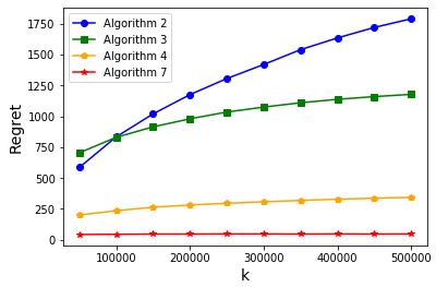
for all i∈{1,2,…,1000}i\in\{1,2,\dots,1000\}, j∈{1,2,…,1000}j\in\{1,2,\dots,1000\}. We then fix revenue vector rr and the bill-of-material matrix AA in the experiments. We set C=0.8​kC=0.8k, and test our Algorithm 2, Algorithm 3 and Algorithm 4 under horizon length k=5×104,10×104,…,5×105k=5\times 10^{4},10\times 10^{4},\dots,5\times 10^{5}.

Refer to caption
Figure 5: Regret of Algorithm 2, Algorithm 3, Algorithm 4, Algorithm 7 for k=5×104,10×104,…,5×105k=5\times 10^{4},10\times 10^{4},\dots,5\times 10^{5}.

Figure 5 shows the average regret of Algorithm 2, Algorithm 3, Algorithm 4, Algorithm 7 over 10001000 experiments with the fixed revenue vector rr and the fixed bill-of-material matrix AA. The regret results of different algorithms are aligned with those in the single-resource case: 1) all algorithms show convergence in regret as k→∞k\rightarrow\infty; 2) among Algorithm 2, Algorithm 3 and Algorithm 4, Algorithm 4 performs the best and Algorithm 2 performs the worst; 3) Algorithm 7 improves the performance of Algorithm 4 by warm-starting each epoch with the bid prices from the last epoch.

6 Conclusion

In this paper, we study the quantity-based network revenue management problem and propose near-optimal algorithms with provable performance guarantees. In particular, our algorithm is the first to achieve o⁡(T)o(\sqrt{T}) regret bound among all the algorithms that do not solve any deterministic linear programs. Moreover, our algorithms are amenable to implementations in online platforms as the algorithms do not perform matrix inversions, and their memory consumption does not scale with the online traffic.

References

  • Agrawal and Devanur (2016) Agrawal S, Devanur N (2016) Linear contextual bandits with knapsacks. Advances in Neural Information Processing Systems, 3450–3458.
  • Agrawal and Devanur (2014) Agrawal S, Devanur NR (2014) Fast algorithms for online stochastic convex programming. Proceedings of the twenty-sixth annual ACM-SIAM symposium on Discrete algorithms, 1405–1424 (SIAM).
  • Agrawal et al. (2014) Agrawal S, Wang Z, Ye Y (2014) A dynamic near-optimal algorithm for online linear programming. Operations Research 62(4):876–890.
  • Airbnb (2020) Airbnb (2020) Airbnb q4 2020 shareholder letter. https://investors.airbnb.com/financials/default.aspx#quarterly, accessed: 2020-12-31.
  • Arlotto and Gurvich (2019) Arlotto A, Gurvich I (2019) Uniformly bounded regret in the multisecretary problem. Stochastic Systems 9(3):231–260.
  • Arlotto and Xie (2018) Arlotto A, Xie X (2018) Logarithmic regret in the dynamic and stochastic knapsack problem. arXiv preprint arXiv:1809.02016 .
  • Atar and Reiman (2013) Atar R, Reiman MI (2013) Asymptotically optimal dynamic pricing for network revenue management. Stochastic Systems 2(2):232–276.
  • Balseiro et al. (2020a) Balseiro S, Lu H, Mirrokni V (2020a) The best of many worlds: Dual mirror descent for online allocation problems. arXiv preprint arXiv:2011.10124 .
  • Balseiro et al. (2020b) Balseiro S, Lu H, Mirrokni V (2020b) Dual mirror descent for online allocation problems. International Conference on Machine Learning, 613–628 (PMLR).
  • Bumpensanti and Wang (2020) Bumpensanti P, Wang H (2020) A re-solving heuristic with uniformly bounded loss for network revenue management. Management Science .
  • Chen and Farias (2013) Chen Y, Farias VF (2013) Simple policies for dynamic pricing with imperfect forecasts. Operations Research 61(3):612–624.
  • Devanur and Hayes (2009) Devanur NR, Hayes TP (2009) The adwords problem: online keyword matching with budgeted bidders under random permutations. Proceedings of the 10th ACM conference on Electronic commerce, 71–78.
  • Gallego and Van Ryzin (1994) Gallego G, Van Ryzin G (1994) Optimal dynamic pricing of inventories with stochastic demand over finite horizons. Management Science 40(8):999–1020.
  • Gallego and Van Ryzin (1997) Gallego G, Van Ryzin G (1997) A multiproduct dynamic pricing problem and its applications to network yield management. Operations research 45(1):24–41.
  • Hazan (2019) Hazan E (2019) Introduction to online convex optimization. arXiv preprint arXiv:1909.05207 .
  • Jasin and Kumar (2012) Jasin S, Kumar S (2012) A re-solving heuristic with bounded revenue loss for network revenue management with customer choice. Mathematics of Operations Research 37(2):313–345.
  • Li et al. (2020) Li X, Sun C, Ye Y (2020) Simple and fast algorithm for binary integer and online linear programming. arXiv preprint arXiv:2003.02513 .
  • Li and Yao (2004) Li X, Yao DD (2004) Control and pricing in stochastic networks with concurrent resource occupancy. ACM SIGMETRICS Performance Evaluation Review 32(2):50–52.
  • Li and Ye (2019) Li X, Ye Y (2019) Online linear programming: Dual convergence, new algorithms, and regret bounds. arXiv preprint arXiv:1909.05499 .
  • Maglaras and Meissner (2006) Maglaras C, Meissner J (2006) Dynamic pricing strategies for multiproduct revenue management problems. Manufacturing & Service Operations Management 8(2):136–148.
  • Medium (2018) Medium (2018) Online travel metrics: Traffic, marketing, channels, mobile. , accessed: 2020-12-31.
  • Reiman and Wang (2008) Reiman MI, Wang Q (2008) An asymptotically optimal policy for a quantity-based network revenue management problem. Mathematics of Operations Research 33(2):257–282.
  • Talluri and Van Ryzin (1998) Talluri K, Van Ryzin G (1998) An analysis of bid-price controls for network revenue management. Management Science 44(11-part-1):1577–1593.
  • Talluri and Van Ryzin (2004) Talluri K, Van Ryzin G (2004) Revenue management under a general discrete choice model of consumer behavior. Management Science 50(1):15–33.
  • Vera and Banerjee (2020) Vera A, Banerjee S (2020) The bayesian prophet: A low-regret framework for online decision making. Management Science .
  • Williamson (1992) Williamson EL (1992) Airline network seat inventory control: Methodologies and revenue impacts. Ph.D. thesis, Massachusetts Institute of Technology.
  • Wollmer (1992) Wollmer RD (1992) An airline seat management model for a single leg route when lower fare classes book first. Operations research 40(1):26–37.

Appendix A Proofs for Algorithm 2

Without loss of generality, we prove lemmas, propositions and theorems with respect to Algorithm 2 with

t1=1,t2=t∗t_{1}=1,\quad t_{2}=t^{*}

and initial capacity CC, for any t∗∈{1,2,…,T}t^{*}\in\{1,2,\ldots,T\}. Let Cmax=maxi∈[m]⁡CiC_{\text{max}}=\max_{i\in[m]}C_{i} and Cmin=mini∈[m]⁡CiC_{\text{min}}=\min_{i\in[m]}C_{i} be the maximum and minimum of the initial capacity values, respectively. Then other notations in Algorithm 2 become

L=T−t1+1=T,L=T-t_{1}+1=T,
θ¯=CmaxCmin​∑i=1mαi¯,\bar{\theta}=\frac{C_{\max}}{C_{\min}}\sum_{i=1}^{m}\bar{\alpha_{i}}, (23)
D=θ¯​m=CmaxCmin​∑i=1mαi¯​m,D=\bar{\theta}\sqrt{m}=\frac{C_{\max}}{C_{\min}}\sum_{i=1}^{m}\bar{\alpha_{i}}\sqrt{m}, (24)
G=CmaxT​m+a¯​m,G=\frac{C_{\max}}{T}\sqrt{m}+\bar{a}\sqrt{m}, (25)

and

gt​(θ)=∑i∈[m]θi​(CiT−yt​ai,j⁡(t)).g_{t}(\theta)=\sum_{i\in[m]}\theta_{i}\left(\frac{C_{i}}{T}-y_{t}a_{i,j(t)}\right).

Suppose Algorithm 2 stops at the beginning of period τ\tau. In particular, when the algorithm stops due to insufficient remaining resources at the beginning of period tt, namely due to some jj that violates Aj≤B⁡(t)A_{j}\leq B(t), we have τ=t\tau=t. Otherwise, we have τ=t∗+1\tau=t^{*}+1.

A.1 Lemma A.1

Lemma A.1

There exists some random variable I∈[m]I\in[m] such that

∑t=1τ−1gt​(θ(t))≤α​τ−1T​CI−α​t∗T​CI+α​a¯+(ρ1​Cmax2Cmin​T+ρ0​CmaxCmin)​t∗\sum_{t=1}^{\tau-1}g_{t}(\theta^{(t)})\leq\alpha\frac{\tau-1}{T}C_{I}-\alpha\frac{t^{*}}{T}C_{I}+\alpha\bar{a}+\left(\rho_{1}\frac{C_{\text{max}}^{2}}{C_{\text{min}}T}+\rho_{0}\frac{C_{\text{max}}}{C_{\text{min}}}\right)\sqrt{t^{*}}

almost surely, for any α∈[0,θ¯]\alpha\in[0,\bar{\theta}], where a¯\bar{a} is defined in (13), and ρ0,ρ1>0\rho_{0},\rho_{1}>0 do not depend on CmaxC_{\text{max}}, CminC_{\text{min}} or TT.

Proof A.2

Proof of Lemma A.1.

According to the OGD property in Proposition 3.1, we have

∑t=1τ−1gt​(θ(t))≤∑t=1τ−1gt​(θ)+ρ​τ−1\sum_{t=1}^{\tau-1}g_{t}(\theta^{(t)})\leq\sum_{t=1}^{\tau-1}g_{t}(\theta)+\rho\sqrt{\tau-1} (26)

for all θ∈[0,θ¯]m\theta\in[0,\bar{\theta}]^{m}, where ρ=32​G​D\rho=\frac{3}{2}GD.

Consider the following two cases.

  • •

    Case 1: τ−1<t∗\tau-1<t^{*}. Let 𝐞i\mathbf{e}_{i} denote a unit vector with the ii-th component being one. For any α∈[0,θ¯]\alpha\in[0,\bar{\theta}], since α⋅t∗T⋅𝐞i∈[0,θ¯]m\alpha\cdot\frac{t^{*}}{T}\cdot\mathbf{e}_{i}\in[0,\bar{\theta}]^{m}, we use (26) to obtain

    ∑t=1τ−1gt​(θ(t))≤∑t=1τ−1gt​(α⋅t∗T⋅𝐞i)+ρ​τ−1\sum_{t=1}^{\tau-1}g_{t}(\theta^{(t)})\leq\sum_{t=1}^{\tau-1}g_{t}(\alpha\cdot\frac{t^{*}}{T}\cdot\mathbf{e}_{i})+\rho\sqrt{\tau-1} (27)

    for all i∈[m]i\in[m].

    Conditioned on τ−1<t∗\tau-1<t^{*}, since some resource II has been depleted before the end of the horizon, we have ∑t=1τ−1yt​aI,j⁡(t)≥CI−maxj∈[n]⁡aI,j≥CI−a¯\sum_{t=1}^{\tau-1}y_{t}a_{I,j(t)}\geq C_{I}-\max_{j\in[n]}a_{I,j}\geq C_{I}-\bar{a}, and

    ∑t=1τ−1gt​(α⋅t∗T⋅𝐞I)\displaystyle\sum_{t=1}^{\tau-1}g_{t}(\alpha\cdot\frac{t^{*}}{T}\cdot\mathbf{e}_{I}) =∑t=1τ−1α​t∗T​(CIT−yt​aI,j⁡(t))\displaystyle=\sum_{t=1}^{\tau-1}\alpha\frac{t^{*}}{T}\left(\frac{C_{I}}{T}-y_{t}a_{I,j(t)}\right)
    =∑t=1τ−1α​t∗T​CIT−∑t=1τ−1yt​α​t∗T​aI,j⁡(t)\displaystyle=\sum_{t=1}^{\tau-1}\alpha\frac{t^{*}}{T}\frac{C_{I}}{T}-\sum_{t=1}^{\tau-1}y_{t}\alpha\frac{t^{*}}{T}a_{I,j(t)}
    =(τ−1)​α​t∗T​CIT−α​t∗T​∑t=1τ−1yt​aI,j⁡(t)\displaystyle=(\tau-1)\alpha\frac{t^{*}}{T}\frac{C_{I}}{T}-\alpha\frac{t^{*}}{T}\sum_{t=1}^{\tau-1}y_{t}a_{I,j(t)}
    ≤(τ−1)​α​t∗T​CIT−α​t∗T​(CI−a¯)\displaystyle\leq(\tau-1)\alpha\frac{t^{*}}{T}\frac{C_{I}}{T}-\alpha\frac{t^{*}}{T}(C_{I}-\bar{a})
    =(τ−1)​α​t∗T​CIT−α​t∗T​CI+α​t∗T​a¯\displaystyle=(\tau-1)\alpha\frac{t^{*}}{T}\frac{C_{I}}{T}-\alpha\frac{t^{*}}{T}C_{I}+\alpha\frac{t^{*}}{T}\bar{a}
    ≤(τ−1)​α​CIT−α​t∗T​CI+α​a¯,\displaystyle\leq(\tau-1)\alpha\frac{C_{I}}{T}-\alpha\frac{t^{*}}{T}C_{I}+\alpha\bar{a}, (28)

    where the first equality is by definition of gt​(⋅)g_{t}(\cdot), the first inequality is because resource II is depleted by time τ−1\tau-1, and the last inequality follows since t∗≤Tt^{*}\leq T.

    Combining (27) and (28), we obtain

    ∑t=1τ−1gt​(θ(t))≤α​τ−1T​CI−α​t∗T​CI+α​a¯+ρ​t∗.\sum_{t=1}^{\tau-1}g_{t}(\theta^{(t)})\leq\alpha\frac{\tau-1}{T}C_{I}-\alpha\frac{t^{*}}{T}C_{I}+\alpha\bar{a}+\rho\sqrt{t^{*}}.
  • •

    Case 2: τ−1=t∗\tau-1=t^{*}. Again, we use (26) to obtain

    ∑t=1τ−1gt​(θ(t))\displaystyle\sum_{t=1}^{\tau-1}g_{t}(\theta^{(t)}) ≤∑t=1τ−1gk​(0)+ρ​τ−1\displaystyle\leq\sum_{t=1}^{\tau-1}g_{k}(0)+\rho\sqrt{\tau-1}
    =0+ρ​τ−1\displaystyle=0+\rho\sqrt{\tau-1}
    =α​t∗T​CI−α​t∗T​CI+ρ​t∗\displaystyle=\alpha\frac{t^{*}}{T}C_{I}-\alpha\frac{t^{*}}{T}C_{I}+\rho\sqrt{t^{*}}
    =α​τ−1T​CI−α​t∗T​CI+ρ​t∗\displaystyle=\alpha\frac{\tau-1}{T}C_{I}-\alpha\frac{t^{*}}{T}C_{I}+\rho\sqrt{t^{*}}
    ≤α​τ−1T​CI−α​t∗T​CI+α​a¯+ρ​t∗.\displaystyle\leq\alpha\frac{\tau-1}{T}C_{I}-\alpha\frac{t^{*}}{T}C_{I}+\alpha\bar{a}+\rho\sqrt{t^{*}}.

Finally, from (24) and (25), it is easy to derive

ρ=32​G​D=ρ1​Cmax2Cmin​T+ρ0​CmaxCmin,\rho=\frac{3}{2}GD=\rho_{1}\frac{C_{\text{max}}^{2}}{C_{\text{min}}T}+\rho_{0}\frac{C_{\text{max}}}{C_{\text{min}}},

where ρ0\rho_{0} and ρ1\rho_{1} only depend on mm, the coefficients in AA, and r1,…,rnr_{1},\ldots,r_{n}.

This completes the proof. \halmos

A.2 Lemma A.3

Consider the Lagrangian relaxation of (5), namely

𝖫𝖯⁡(θ)=maxxT​∑j∈[n]rj​xj+T​∑i∈[m]θi​(CiT−∑j∈[n]xj​ai​j)s.t.   0≤xj≤λj.∀j∈[n]\displaystyle\begin{split}\mathsf{LP}(\theta)=\max_{x}&\;\;T\sum_{j\in[n]}r_{j}x_{j}+T\sum_{i\in[m]}\theta_{i}(\frac{C_{i}}{T}-\sum_{j\in[n]}x_{j}a_{ij})\\ \text{s.t. }&\;\;0\leq x_{j}\leq\lambda_{j}.\quad\forall j\in[n]\end{split} (29)

Define {Mt}t=1,…,τ−1\{M_{t}\}_{t=1,\ldots,\tau-1} as the stochastic process

Mt:=∑s=1t[𝖫𝖯⁡(θ(s))T−ys​rj⁡(s)−gs​(θ(s))].M_{t}:=\sum_{s=1}^{t}\left[\frac{\mathsf{LP}(\theta^{(s)})}{T}-y_{s}r_{j(s)}-g_{s}(\theta^{(s)})\right]. (30)
Lemma A.3

The stochastic process MtM_{t} as defined in (30) is a martingale for t=1,2,…,τ−1t=1,2,\ldots,\tau-1.

Proof A.4

Proof of Lemma A.3. Let ℋt\mathcal{H}_{t} denote all the information in periods 1,…,t1,\ldots,t where t≤τt\leq\tau.

𝐄⁡[Mt|ℋt−1]\displaystyle\mathbf{E}[M_{t}|\mathcal{H}_{t-1}] =𝐄⁡[∑s=1t[𝖫𝖯⁡(θ(s))T−ys​rj⁡(s)−gs​(θ(s))]|ℋt−1]\displaystyle=\mathbf{E}\left[\sum_{s=1}^{t}\left[\frac{\mathsf{LP}(\theta^{(s)})}{T}-y_{s}r_{j(s)}-g_{s}(\theta^{(s)})\right]|\mathcal{H}_{t-1}\right]
=𝐄⁡[∑s=1t−1[𝖫𝖯⁡(θ(s))T−ys​rj⁡(s)−gs​(θ(s))]|ℋt−1]+𝐄⁡[𝖫𝖯⁡(θ(t))T−yt​rj⁡(t)−gt​(θ(t))|ℋt−1].\displaystyle=\mathbf{E}\left[\sum_{s=1}^{t-1}\left[\frac{\mathsf{LP}(\theta^{(s)})}{T}-y_{s}r_{j(s)}-g_{s}(\theta^{(s)})\right]|\mathcal{H}_{t-1}\right]+\mathbf{E}\left[\frac{\mathsf{LP}(\theta^{(t)})}{T}-y_{t}r_{j(t)}-g_{t}(\theta^{(t)})|\mathcal{H}_{t-1}\right].

For the first term, since ∑s=1t−1[𝖫𝖯⁡(θ(s))/T−ys​rj⁡(s)−gs​(θ(s))]∈ℋt−1\sum_{s=1}^{t-1}\left[\mathsf{LP}(\theta^{(s)})/T-y_{s}r_{j(s)}-g_{s}(\theta^{(s)})\right]\in\mathcal{H}_{t-1}, we have

𝐄⁡[∑s=1t−1[𝖫𝖯⁡(θ(s))T−ys​rj⁡(s)−gs​(θ(s))]|ℋt−1]=∑s=1t−1[𝖫𝖯⁡(θ(s))T−ys​rj⁡(s)−gs​(θ(s))]=Mt−1.\mathbf{E}\left[\sum_{s=1}^{t-1}\left[\frac{\mathsf{LP}(\theta^{(s)})}{T}-y_{s}r_{j(s)}-g_{s}(\theta^{(s)})\right]|\mathcal{H}_{t-1}\right]=\sum_{s=1}^{t-1}\left[\frac{\mathsf{LP}(\theta^{(s)})}{T}-y_{s}r_{j(s)}-g_{s}(\theta^{(s)})\right]=M_{t-1}. (31)

For the second term, let xj∗​(θ){x}^{*}_{j}(\theta) for j∈[n]j\in[n] denote an optimal solution to (29). The structure of (29) is simple enough that we can calculate for all j∈[n]j\in[n]:

  • •

    given rj>∑i∈[m]θi(t)​ai​jr_{j}>\sum_{i\in[m]}\theta_{i}^{(t)}a_{ij}, we have xj∗​(θ(t))=λjx^{*}_{j}(\theta^{(t)})=\lambda_{j};

  • •

    given rj≤∑i∈[m]θi(t)​ai​jr_{j}\leq\sum_{i\in[m]}\theta_{i}^{(t)}a_{ij}, we have xj∗​(θ(t))=0x^{*}_{j}(\theta^{(t)})=0.

By definition, we know yt=𝟏​(rj⁡(t)>∑i∈[m]θi(t)​ai,j⁡(t))y_{t}=\mathbf{1}(r_{j(t)}>\sum_{i\in[m]}\theta_{i}^{(t)}a_{i,j(t)}). Therefore, we have yt=xj⁡(t)∗​(θ(t))/λj⁡(t)y_{t}=x^{*}_{j(t)}(\theta^{(t)})/\lambda_{j(t)}.

Notice that θ(t)∈ℋt−1\theta^{(t)}\in\mathcal{H}_{t-1}, since the value of θ(t)\theta^{(t)} has been determined at the end of period t−1t-1. Thus, by taking expectation over all customer types j∈[n]j\in[n] for j⁡(t)j(t), we have

𝐄⁡[yt​rj⁡(t)|ℋt−1]\displaystyle\mathbf{E}[y_{t}r_{j(t)}|\mathcal{H}_{t-1}]
=\displaystyle= 𝐄⁡[xj⁡(t)∗​(θ(t))λj⁡(t)​rj⁡(t)|ℋt−1]\displaystyle\mathbf{E}[\frac{x^{*}_{j(t)}(\theta^{(t)})}{\lambda_{j(t)}}r_{j(t)}|\mathcal{H}_{t-1}]
=\displaystyle= ∑j∈[n]𝐏⁡(j⁡(t)=j)​xj∗​(θ(t))λj​rj\displaystyle\sum_{j\in[n]}\mathbf{P}(j(t)=j)\frac{x^{*}_{j}(\theta^{(t)})}{\lambda_{j}}r_{j}
=\displaystyle= ∑j∈[n]λj​xj∗​(θ(t))λj​rj\displaystyle\sum_{j\in[n]}\lambda_{j}\frac{x^{*}_{j}(\theta^{(t)})}{\lambda_{j}}r_{j}
=\displaystyle= ∑j∈[n]rj​xj∗​(θ(t)).\displaystyle\sum_{j\in[n]}r_{j}x^{*}_{j}(\theta^{(t)}). (32)
𝐄⁡[gt​(θ(t))|ℋt−1]\displaystyle\mathbf{E}[g_{t}(\theta^{(t)})|\mathcal{H}_{t-1}]
=\displaystyle= 𝐄⁡[∑i∈[m]θi(t)​(CiT−yt​ai,j⁡(t))|ℋt−1]\displaystyle\mathbf{E}[\sum_{i\in[m]}\theta_{i}^{(t)}\left(\frac{C_{i}}{T}-y_{t}a_{i,j(t)}\right)|\mathcal{H}_{t-1}]
=\displaystyle= ∑i∈[m]θi(t)​CiT−∑i∈[m]θi(t)​𝐄​[yt​ai,j⁡(t)|ℋt−1]\displaystyle\sum_{i\in[m]}\theta_{i}^{(t)}\frac{C_{i}}{T}-\sum_{i\in[m]}\theta_{i}^{(t)}\mathbf{E}[y_{t}a_{i,j(t)}|\mathcal{H}_{t-1}]
=\displaystyle= ∑i∈[m]θi(t)​CiT−∑i∈[m]θi(t)​𝐄​[xj⁡(t)∗​(θ(t))λj⁡(t)​ai,j⁡(t)|ℋt−1]\displaystyle\sum_{i\in[m]}\theta_{i}^{(t)}\frac{C_{i}}{T}-\sum_{i\in[m]}\theta_{i}^{(t)}\mathbf{E}[\frac{x^{*}_{j(t)}(\theta^{(t)})}{\lambda_{j(t)}}a_{i,j(t)}|\mathcal{H}_{t-1}]
=\displaystyle= ∑i∈[m]θi(t)​CiT−∑i∈[m]θi(t)​∑j∈[n]𝐏⁡(j⁡(t)=j)​xj∗​(θ(t))λj​ai,j\displaystyle\sum_{i\in[m]}\theta_{i}^{(t)}\frac{C_{i}}{T}-\sum_{i\in[m]}\theta_{i}^{(t)}\sum_{j\in[n]}\mathbf{P}(j(t)=j)\frac{x^{*}_{j}(\theta^{(t)})}{\lambda_{j}}a_{i,j}
=\displaystyle= ∑i∈[m]θi(t)​CiT−∑i∈[m]θi(t)​∑j∈[n]λj​xj∗​(θ(t))λj​ai,j\displaystyle\sum_{i\in[m]}\theta_{i}^{(t)}\frac{C_{i}}{T}-\sum_{i\in[m]}\theta_{i}^{(t)}\sum_{j\in[n]}\lambda_{j}\frac{x^{*}_{j}(\theta^{(t)})}{\lambda_{j}}a_{i,j}
=\displaystyle= ∑i∈[m]θi(t)​CiT−∑i∈[m]∑j∈[n]θi(t)​xj∗​(θ(t))​ai​j.\displaystyle\sum_{i\in[m]}\theta_{i}^{(t)}\frac{C_{i}}{T}-\sum_{i\in[m]}\sum_{j\in[n]}\theta_{i}^{(t)}x^{*}_{j}(\theta^{(t)})a_{ij}. (33)

Combining (32) and (33), we have

𝐄⁡[yt​rj⁡(t)+gt​(θ(t))|ℋt−1]=∑j∈[n]rj​xj∗​(θ(t))+∑i∈[m]θi(t)​CiT−∑i∈[m]∑j∈[n]θi(t)​xj∗​(θ(t))​ai​j=𝖫𝖯⁡(θ(t))T.\mathbf{E}[y_{t}r_{j(t)}+g_{t}(\theta^{(t)})|\mathcal{H}_{t-1}]=\sum_{j\in[n]}r_{j}x^{*}_{j}(\theta^{(t)})+\sum_{i\in[m]}\theta_{i}^{(t)}\frac{C_{i}}{T}-\sum_{i\in[m]}\sum_{j\in[n]}\theta_{i}^{(t)}x^{*}_{j}(\theta^{(t)})a_{ij}=\frac{\mathsf{LP}(\theta^{(t)})}{T}. (34)

Hence, we have

𝐄⁡[[𝖫𝖯⁡(θ(t))T−yt​rj⁡(t)−gt​(θ(t))]|ℋt−1]=0\mathbf{E}\left[\left[\frac{\mathsf{LP}(\theta^{(t)})}{T}-y_{t}r_{j(t)}-g_{t}(\theta^{(t)})\right]\big|\mathcal{H}_{t-1}\right]=0 (35)

Combining (31) and (35), we have

𝐄⁡[Mt|ℋt−1]=Mt−1,\mathbf{E}[M_{t}|\mathcal{H}_{t-1}]=M_{t-1}, (36)

which shows that MtM_{t} is a martingale. \halmos

A.3 Lemma A.5

Lemma A.5 (Azuma’s Inequality)

Suppose MtM_{t} is a martingale, and

|Mt−Mt−1|≤ct|M_{t}-M_{t-1}|\leq c_{t} (37)

almost surely, then for any positive integer NN and any positive a∈ℝa\in\mathbb{R}, we have

𝐏⁡(Mt≤a)≥1−exp⁡(−a22​∑k=1tck2).\mathbf{P}(M_{t}\leq a)\geq 1-\exp\left(-\frac{a^{2}}{2\sum_{k=1}^{t}c_{k}^{2}}\right). (38)

A.4 Lemma A.6

Lemma A.6

Consider MtM_{t} as defined in (30). With probability at least 1−1K1-\frac{1}{K}, we have

Mt≤(ρ2​CmaxCmin+ρ3)​τ−1​(log⁡K)12M_{t}\leq\left(\rho_{2}\frac{C_{\text{max}}}{C_{\text{min}}}+\rho_{3}\right)\sqrt{\tau-1}(\log K)^{\frac{1}{2}}

for all t=1,2,…,τ−1t=1,2,\ldots,\tau-1, where ρ2\rho_{2} and ρ3\rho_{3} do not depend on CmaxC_{\text{max}}, CminC_{\text{min}} or KK.

Proof A.7

Proof of Lemma A.6. We apply Azuma’s inequality to obtain

𝐏⁡(Mt≤(ρ2​CmaxCmin+ρ3)​τ−1​(log⁡K)12)≥1−exp⁡(−(ρ2​CmaxCmin+ρ3)2​(τ−1)​log⁡K2​∑k=1tc2),\mathbf{P}\left(M_{t}\leq\left(\rho_{2}\frac{C_{\text{max}}}{C_{\text{min}}}+\rho_{3}\right)\sqrt{\tau-1}(\log K)^{\frac{1}{2}}\right)\geq 1-\exp\left(-\frac{\left(\rho_{2}\frac{C_{\text{max}}}{C_{\text{min}}}+\rho_{3}\right)^{2}(\tau-1)\log K}{2\sum_{k=1}^{t}c^{2}}\right), (39)

where cc satisfies |Mk−Mk−1|≤ck|M_{k}-M_{k-1}|\leq c_{k}. We next find the proper values of ρ2\rho_{2}, ρ3\rho_{3} and cc.

Let xj∗​(θ){x}^{*}_{j}(\theta) for j∈[n]j\in[n] denote an optimal solution to 𝖫𝖯⁡(θ)\mathsf{LP}(\theta) in (29). We have 0≤xj∗​(θ)≤λj0\leq{x}^{*}_{j}(\theta)\leq\lambda_{j}.

By definition of MtM_{t}, we know

Mt−\displaystyle M_{t}- Mt−1=𝖫𝖯⁡(θ(t))T−yt​rj⁡(t)−gt​(θ(t))\displaystyle M_{t-1}=\frac{\mathsf{LP}(\theta^{(t)})}{T}-y_{t}r_{j(t)}-g_{t}(\theta^{(t)})
=1T​(T​∑j∈[n]rj​xj∗​(θ(t))+T​∑i∈[m]θi(t)​(CiT−∑j∈[n]ai​j​xj∗​(θ(t))))−yt​rj⁡(t)−∑i∈[m]θi(t)​(CiT−yt​ai,j⁡(t))\displaystyle=\frac{1}{T}\left(T\sum_{j\in[n]}r_{j}x_{j}^{*}(\theta^{(t)})+T\sum_{i\in[m]}\theta_{i}^{(t)}(\frac{C_{i}}{T}-\sum_{j\in[n]}a_{ij}{x}^{*}_{j}(\theta^{(t)}))\right)-y_{t}r_{j(t)}-\sum_{i\in[m]}\theta_{i}^{(t)}\left(\frac{C_{i}}{T}-y_{t}a_{i,j(t)}\right)
=∑j∈[n]rj​xj∗​(θ(t))−∑i∈[m]θi(t)​∑j∈[n]ai​j​xj∗​(θ(t))−yt​rj⁡(t)+yt​∑i∈[m]ai,j⁡(t)​θi(t).\displaystyle=\sum_{j\in[n]}r_{j}{x}^{*}_{j}(\theta^{(t)})-\sum_{i\in[m]}\theta_{i}^{(t)}\sum_{j\in[n]}a_{ij}{x}^{*}_{j}(\theta^{(t)})-y_{t}r_{j(t)}+y_{t}\sum_{i\in[m]}a_{i,j(t)}\theta_{i}^{(t)}.

Recall a¯=maxi∈[m],j∈[n]⁡ai​j\bar{a}=\max_{i\in[m],j\in[n]}a_{ij} and θ(t)∈[0,θ¯]m\theta^{(t)}\in[0,\bar{\theta}]^{m}. We remove the non-positive terms in the above equation to obtain

Mt−Mt−1\displaystyle M_{t}-M_{t-1} ≤∑j∈[n]rj​xj∗​(θ(t))+yt​∑i∈[m]ai,j⁡(t)​θi(t)\displaystyle\leq\sum_{j\in[n]}r_{j}{x}^{*}_{j}(\theta^{(t)})+y_{t}\sum_{i\in[m]}a_{i,j(t)}\theta_{i}^{(t)}
≤‖r‖∞​∑j∈[n]xj∗​(θ(t))+m​a¯​θ¯\displaystyle\leq\|r\|_{\infty}\sum_{j\in[n]}{x}^{*}_{j}(\theta^{(t)})+m\bar{a}\bar{\theta}
≤‖r‖∞​∑j∈[n]λj+m​a¯​θ¯\displaystyle\leq\|r\|_{\infty}\sum_{j\in[n]}\lambda_{j}+m\bar{a}\bar{\theta}
=‖r‖∞+m​a¯​θ¯.\displaystyle=\|r\|_{\infty}+m\bar{a}\bar{\theta}. (40)

On the other hand, we remove the non-negative terms to obtain

Mt−Mt−1\displaystyle M_{t}-M_{t-1} ≥−∑i∈[m]θi(t)∑j∈[n]ai​jxj∗(θ(t))−ytrj⁡(t)\displaystyle\geq-\sum_{i\in[m]}\theta_{i}^{(t)}\sum_{j\in[n]}a_{ij}{x}^{*}_{j}(\theta^{(t)})-y_{t}r_{j(t)}
≥−mθ¯a¯∑j∈[n]xj∗(θ(t))−∥r∥∞\displaystyle\geq-m\bar{\theta}\bar{a}\sum_{j\in[n]}{x}^{*}_{j}(\theta^{(t)})-\|r\|_{\infty}
≥−mθ¯a¯∑j∈[n]λj−∥r∥∞\displaystyle\geq-m\bar{\theta}\bar{a}\sum_{j\in[n]}\lambda_{j}-\|r\|_{\infty}
≥−m​θ¯​a¯−‖r‖∞.\displaystyle\geq-m\bar{\theta}\bar{a}-\|r\|_{\infty}. (41)

In sum, we have

|Mt−Mt−1|≤‖r‖∞+m​a¯​θ¯.|M_{t}-M_{t-1}|\leq\|r\|_{\infty}+m\bar{a}\bar{\theta}.

We set

c=‖r‖∞+m​a¯​θ¯,c=\|r\|_{\infty}+m\bar{a}\bar{\theta},
ρ2=2​m​a¯​∑i=1mα¯i,\rho_{2}=\sqrt{2}m\bar{a}\sum_{i=1}^{m}\bar{\alpha}_{i},
ρ3=2​‖r‖∞\rho_{3}=\sqrt{2}\|r\|_{\infty}

in Equation (39). We can then simplify (39) to

𝐏⁡(Mt≤(ρ2​CmaxCmin+ρ3)​τ−1​(log⁡K)12)\displaystyle\mathbf{P}\left(M_{t}\leq\left(\rho_{2}\frac{C_{\text{max}}}{C_{\text{min}}}+\rho_{3}\right)\sqrt{\tau-1}(\log K)^{\frac{1}{2}}\right) ≥1−exp⁡(−(ρ2​CmaxCmin+ρ3)2​(τ−1)​log⁡K2​∑k=1t(‖r‖∞+m​a¯​θ¯)2)\displaystyle\geq 1-\exp\left(-\frac{\left(\rho_{2}\frac{C_{\text{max}}}{C_{\text{min}}}+\rho_{3}\right)^{2}(\tau-1)\log K}{2\sum_{k=1}^{t}(\|r\|_{\infty}+m\bar{a}\bar{\theta})^{2}}\right)
≥1−exp⁡(−(2​m​a¯​CmaxCmin​∑i=1mαi¯+2​‖r‖∞)2​(τ−1)​log⁡K2​∑k=1t(‖r‖∞+m​a¯​CmaxCmin​∑i=1mαi¯)2)\displaystyle\geq 1-\exp\left(-\frac{\left(\sqrt{2}m\bar{a}\frac{C_{\max}}{C_{\min}}\sum_{i=1}^{m}\bar{\alpha_{i}}+\sqrt{2}\|r\|_{\infty}\right)^{2}(\tau-1)\log K}{2\sum_{k=1}^{t}(\|r\|_{\infty}+m\bar{a}\frac{C_{\max}}{C_{\min}}\sum_{i=1}^{m}\bar{\alpha_{i}})^{2}}\right)
=1−exp⁡(−τ−1t​log⁡K)≥1−1K\displaystyle=1-\exp\left(-\frac{\tau-1}{t}\log K\right)\geq 1-\frac{1}{K} (42)

for all t=1,2,…,τ−1t=1,2,\ldots,\tau-1.

This completes the proof. \halmos

A.5 Lemma A.8

Lemma A.8

Given the definition of α¯\bar{\alpha} in (23), we have

VDLPCmin≤θ¯.\frac{V^{\text{{DLP}}}}{C_{\min}}\leq\bar{\theta}.
Proof A.9

Proof of Lemma A.8. Consider 𝖫𝖯⁡(θ)\mathsf{LP}(\theta) as defined in (29). By weak duality, we have 𝖫𝖯⁡(θ)≥VDLP\mathsf{LP}(\theta)\geq V^{\text{{DLP}}} for any θ≥0\theta\geq 0. Recall that αi¯=maxj:ai​j≠0rj/ai​j\bar{\alpha_{i}}=\max_{j:a_{ij}\neq 0}r_{j}/a_{ij} and θ¯=∑i∈[m]αi¯​Cmax/Cmin.\bar{\theta}=\sum_{i\in[m]}\bar{\alpha_{i}}C_{\max}/C_{\min}. By definition, we know

αi¯​ai​j≥rj,∀j​ and ​ai​j≠0.\bar{\alpha_{i}}a_{ij}\geq r_{j},\;\forall j\text{ and }a_{ij}\neq 0.

Now let θi=αi¯\theta_{i}=\bar{\alpha_{i}} for i∈[m]i\in[m] and let x∗​(θ)x^{*}(\theta) denote an optimal solution to (29). We can derive

VDLP≤𝖫𝖯⁡(θ)\displaystyle V^{\text{{DLP}}}\leq\mathsf{LP}(\theta) =T​∑j∈[n](rj−∑i∈[m]αi¯​ai​j)​xj∗​(θ)+∑i∈[m]αi¯​Ci≤∑i∈[m]αi¯​Cmax.\displaystyle=T\sum_{j\in[n]}(r_{j}-\sum_{i\in[m]}\bar{\alpha_{i}}a_{ij})x_{j}^{*}(\theta)+\sum_{i\in[m]}\bar{\alpha_{i}}C_{i}\leq\sum_{i\in[m]}\bar{\alpha_{i}}C_{\max}.

The last inequality follows since 1) the first term on the left hand side is non-positive, and 2) Ci≤CmaxC_{i}\leq C_{\max} for all i∈[m]i\in[m] by definition. Divide both sides by CminC_{\min}, and we obtain the result. \halmos

A.6 Proposition 3.2

Now we prove the following proposition, which is more general than Proposition 3.2. Let V𝖠𝖫𝖦𝟤​(t∗)V^{\mathsf{ALG2}}(t^{*}) denote the revenue of Algorithm 2 with start time t1=1t_{1}=1, end time t2=t∗t_{2}=t^{*} and initial capacity CC.

Proposition A.10

With probability at least 1−1K1-\frac{1}{K} where K=Ω⁡(T)K=\Omega(T), we have

t∗T​VDLP−V𝖠𝖫𝖦𝟤​(t∗)≤(ρ2​CmaxCmin+ρ3)​t∗​(log⁡K)12+(ρ1​Cmax2Cmin​T+ρ0​CmaxCmin)​t∗+ρ4​CmaxCmin,\frac{t^{*}}{T}V^{\text{{DLP}}}-V^{\mathsf{ALG2}}(t^{*})\leq\left(\rho_{2}\frac{C_{\text{max}}}{C_{\text{min}}}+\rho_{3}\right)\sqrt{t^{*}}(\log K)^{\frac{1}{2}}+\left(\rho_{1}\frac{C_{\text{max}}^{2}}{C_{\text{min}}T}+\rho_{0}\frac{C_{\text{max}}}{C_{\text{min}}}\right)\sqrt{t^{*}}+\rho_{4}\frac{C_{\text{max}}}{C_{\text{min}}}, (43)

where ρ0,ρ1,…,ρ4\rho_{0},\rho_{1},\ldots,\rho_{4} do not depend on CmaxC_{\text{max}}, CminC_{\text{min}}, TT or KK.

Proof A.11

Proof of Proposition A.10.

By Proposition A.6 and definition of MtM_{t}, we have with probability at least 1−1K1-\frac{1}{K} that

∑s=1t[𝖫𝖯⁡(θ(s))T−ys​rj⁡(s)−gs​(θ(s))]≤(ρ2​CmaxCmin+ρ3)​τ−1​(log⁡K)12.\sum_{s=1}^{t}\left[\frac{\mathsf{LP}(\theta^{(s)})}{T}-y_{s}r_{j(s)}-g_{s}(\theta^{(s)})\right]\leq\left(\rho_{2}\frac{C_{\text{max}}}{C_{\text{min}}}+\rho_{3}\right)\sqrt{\tau-1}(\log K)^{\frac{1}{2}}. (44)

By Lemma A.1, we know there exists some random variable I∈[m]I\in[m] such that

∑t=1τ−1gt​(θ(t))≤α​τ−1T​CI−α​t∗T​CI+α​a¯+(ρ1​Cmax2Cmin​T+ρ0​CmaxCmin)​t∗\sum_{t=1}^{\tau-1}g_{t}(\theta^{(t)})\leq\alpha\frac{\tau-1}{T}C_{I}-\alpha\frac{t^{*}}{T}C_{I}+\alpha\bar{a}+\left(\rho_{1}\frac{C_{\text{max}}^{2}}{C_{\text{min}}T}+\rho_{0}\frac{C_{\text{max}}}{C_{\text{min}}}\right)\sqrt{t^{*}} (45)

almost surely, for any α∈[0,θ¯]\alpha\in[0,\bar{\theta}].

Recall that 𝖫𝖯⁡(θ)\mathsf{LP}(\theta) is the Lagrangian relaxation defined in Equation (29). By weak duality, we have 𝖫𝖯⁡(θ)≥VDLP\mathsf{LP}(\theta)\geq V^{\text{DLP}} for all θ≥0\theta\geq 0. Combining this with (44) and (45), we can derive that with probability at least 1−1K1-\frac{1}{K} that

τ−1T​VDLP\displaystyle\frac{\tau-1}{T}V^{\text{DLP}} ≤∑t=1τ−1𝖫𝖯⁡(θ(t))T\displaystyle\leq\sum_{t=1}^{\tau-1}\frac{\mathsf{LP}(\theta^{(t)})}{T}
≤∑t=1τ−1yt​rj⁡(t)+∑t=1τ−1gt​(θ(t))+(ρ2​CmaxCmin+ρ3)​t∗​(log⁡K)12\displaystyle\leq\sum_{t=1}^{\tau-1}y_{t}r_{j(t)}+\sum_{t=1}^{\tau-1}g_{t}(\theta^{(t)})+\left(\rho_{2}\frac{C_{\text{max}}}{C_{\text{min}}}+\rho_{3}\right)\sqrt{t^{*}}(\log K)^{\frac{1}{2}}
≤∑t=1τ−1yt​rj⁡(t)+α​τ−1T​CI−α​t∗T​CI+α​a¯+(ρ1​Cmax2Cmin​T+ρ0​CmaxCmin)​t∗+(ρ2​CmaxCmin+ρ3)​t∗​(log⁡K)12\displaystyle\leq\sum_{t=1}^{\tau-1}y_{t}r_{j(t)}+\alpha\frac{\tau-1}{T}C_{I}-\alpha\frac{t^{*}}{T}C_{I}+\alpha\bar{a}+\left(\rho_{1}\frac{C_{\text{max}}^{2}}{C_{\text{min}}T}+\rho_{0}\frac{C_{\text{max}}}{C_{\text{min}}}\right)\sqrt{t^{*}}+\left(\rho_{2}\frac{C_{\text{max}}}{C_{\text{min}}}+\rho_{3}\right)\sqrt{t^{*}}(\log K)^{\frac{1}{2}}

for any α∈[0,θ¯]\alpha\in[0,\bar{\theta}]. Now we set α=θ¯\alpha=\bar{\theta}. By Lemma A.8, we know α⋅CI=θ¯⋅CI≥VDLP\alpha\cdot C_{I}=\bar{\theta}\cdot C_{I}\geq V^{\text{{DLP}}}. We continue to derive

τ−1T​VDLP\displaystyle\frac{\tau-1}{T}V^{\text{DLP}}
≤\displaystyle\leq ∑t=1τ−1yt​rj⁡(t)+θ¯​τ−1T​CI−θ¯​t∗T​CI+θ¯​a¯+(ρ1​Cmax2Cmin​T+ρ0​CmaxCmin)​t∗+(ρ2​CmaxCmin+ρ3)​t∗​(log⁡K)12\displaystyle\sum_{t=1}^{\tau-1}y_{t}r_{j(t)}+\bar{\theta}\frac{\tau-1}{T}C_{I}-\bar{\theta}\frac{t^{*}}{T}C_{I}+\bar{\theta}\bar{a}+\left(\rho_{1}\frac{C_{\text{max}}^{2}}{C_{\text{min}}T}+\rho_{0}\frac{C_{\text{max}}}{C_{\text{min}}}\right)\sqrt{t^{*}}+\left(\rho_{2}\frac{C_{\text{max}}}{C_{\text{min}}}+\rho_{3}\right)\sqrt{t^{*}}(\log K)^{\frac{1}{2}}
≤\displaystyle\leq ∑t=1τ−1yt​rj⁡(t)−θ¯​CI​(t∗T−τ−1T)+θ¯​a¯+(ρ1​Cmax2Cmin​T+ρ0​CmaxCmin)​t∗+(ρ2​CmaxCmin+ρ3)​t∗​(log⁡K)12\displaystyle\sum_{t=1}^{\tau-1}y_{t}r_{j(t)}-\bar{\theta}C_{I}\left(\frac{t^{*}}{T}-\frac{\tau-1}{T}\right)+\bar{\theta}\bar{a}+\left(\rho_{1}\frac{C_{\text{max}}^{2}}{C_{\text{min}}T}+\rho_{0}\frac{C_{\text{max}}}{C_{\text{min}}}\right)\sqrt{t^{*}}+\left(\rho_{2}\frac{C_{\text{max}}}{C_{\text{min}}}+\rho_{3}\right)\sqrt{t^{*}}(\log K)^{\frac{1}{2}}
≤\displaystyle\leq ∑t=1τ−1yt​rj⁡(t)−VDLP​(t∗T−τ−1T)+θ¯​a¯+(ρ1​Cmax2Cmin​T+ρ0​CmaxCmin)​t∗+(ρ2​CmaxCmin+ρ3)​t∗​(log⁡K)12\displaystyle\sum_{t=1}^{\tau-1}y_{t}r_{j(t)}-V^{\text{{DLP}}}\left(\frac{t^{*}}{T}-\frac{\tau-1}{T}\right)+\bar{\theta}\bar{a}+\left(\rho_{1}\frac{C_{\text{max}}^{2}}{C_{\text{min}}T}+\rho_{0}\frac{C_{\text{max}}}{C_{\text{min}}}\right)\sqrt{t^{*}}+\left(\rho_{2}\frac{C_{\text{max}}}{C_{\text{min}}}+\rho_{3}\right)\sqrt{t^{*}}(\log K)^{\frac{1}{2}}
≤\displaystyle\leq V𝖠𝖫𝖦𝟤​(t∗)−VDLP​(t∗T−τ−1T)+θ¯​a¯+(ρ1​Cmax2Cmin​T+ρ0​CmaxCmin)​t∗+(ρ2​CmaxCmin+ρ3)​t∗​(log⁡K)12.\displaystyle V^{\mathsf{ALG2}}(t^{*})-V^{\text{{DLP}}}\left(\frac{t^{*}}{T}-\frac{\tau-1}{T}\right)+\bar{\theta}\bar{a}+\left(\rho_{1}\frac{C_{\text{max}}^{2}}{C_{\text{min}}T}+\rho_{0}\frac{C_{\text{max}}}{C_{\text{min}}}\right)\sqrt{t^{*}}+\left(\rho_{2}\frac{C_{\text{max}}}{C_{\text{min}}}+\rho_{3}\right)\sqrt{t^{*}}(\log K)^{\frac{1}{2}}.
⟹t∗T​VDLP−V𝖠𝖫𝖦𝟤​(t∗)≤θ¯​a¯+(ρ1​Cmax2Cmin​T+ρ0​CmaxCmin)​t∗+(ρ2​CmaxCmin+ρ3)​t∗​(log⁡K)12.\displaystyle\Longrightarrow\frac{t^{*}}{T}V^{\text{{DLP}}}-V^{\mathsf{ALG2}}(t^{*})\leq\bar{\theta}\bar{a}+\left(\rho_{1}\frac{C_{\text{max}}^{2}}{C_{\text{min}}T}+\rho_{0}\frac{C_{\text{max}}}{C_{\text{min}}}\right)\sqrt{t^{*}}+\left(\rho_{2}\frac{C_{\text{max}}}{C_{\text{min}}}+\rho_{3}\right)\sqrt{t^{*}}(\log K)^{\frac{1}{2}}.

Finally, we set ρ4=∑i=1mαi¯​a¯\rho_{4}=\sum_{i=1}^{m}\bar{\alpha_{i}}\bar{a} to obtain

θ¯​a¯=CmaxCmin​∑i=1mαi¯​a¯=CmaxCmin​ρ4,\bar{\theta}\bar{a}=\frac{C_{\max}}{C_{\min}}\sum_{i=1}^{m}\bar{\alpha_{i}}\bar{a}=\frac{C_{\max}}{C_{\min}}\rho_{4},

which completes the proof.

\halmos

Proposition 3.2 follows from Proposition A.10, where t∗=Tt^{*}=T, K=TK=T and V𝖠𝖫𝖦𝟤​(T)=V𝖠𝖫𝖦𝟤V^{\mathsf{ALG2}}(T)=V^{\mathsf{ALG2}}.

A.7 Lemma 4.2

Recall the definition of 𝖫𝖯⁡(b,v)\mathsf{LP}(b,v) in (17):

𝖫𝖯⁡(b,v):=maxz,ε∑j=1nrj​zjs.t. ∑j=1nAj​zj+εi=b0≤zj≤vj,∀j∈[n]εi≥0,∀i∈[m],\displaystyle\begin{split}\mathsf{LP}(b,v):=\max_{z,\varepsilon}\;\;&\sum_{j=1}^{n}r_{j}z_{j}\\ \text{s.t. }&\sum_{j=1}^{n}A_{j}z_{j}+\varepsilon_{i}=b\\ &0\leq z_{j}\leq v_{j},\;\;\forall j\in[n]\\ &\varepsilon_{i}\geq 0,\;\;\forall i\in[m],\end{split}

and matrix A¯=[A1,…,An,𝐞1,…,𝐞m]\bar{A}=[A_{1},\ldots,A_{n},\mathbf{e}_{1},\ldots,\mathbf{e}_{m}], vector r¯=[r1,…,rn,0,…,0]⊤∈ℝm+n\bar{r}=[r_{1},\ldots,r_{n},0,\ldots,0]^{\top}\in\mathbb{R}^{m+n}.

Proof A.12

Proof of Lemma 4.2. Let w~∗=(z1∗,…,zn∗,ε1∗,…,εm∗)\tilde{w}^{*}=(z^{*}_{1},\ldots,z^{*}_{n},\varepsilon_{1}^{*},\ldots,\varepsilon_{m}^{*}) be an optimal solution to 𝖫𝖯⁡(b,v)\mathsf{LP}(b,v) where εi∗=b−∑j=1nAj​zj∗\varepsilon^{*}_{i}=b-\sum_{j=1}^{n}A_{j}z^{*}_{j} for i∈[m]i\in[m].

First, suppose w~∗\tilde{w}^{*} is a basic feasible solution (BFS). Let B⊂[m+n]B\subset[m+n] be the set of indices for the basic variables, and N:=[m+n]−BN:=[m+n]-B the set of indexes for the non-basic variables. By definition, we know |B|=m|B|=m given there exists mm constraints in (17). In addition, the reduced cost of the basic variables is zero, i.e., we have

r¯l−r¯B⊤​A¯B−1​A¯l=0​ for ​l∈B.\bar{r}_{l}-\bar{r}_{B}^{\top}\bar{A}_{B}^{-1}\bar{A}_{l}=0\text{ for }l\in B.

Consider moving from w~∗\tilde{w}^{*} along the kk-th basic direction dkd_{k} where k∈Nk\in N. By definition, A¯​(w~∗+d)=b\bar{A}(\tilde{w}^{*}+d)=b, which implies A¯​d=A¯B​dB+A¯N​dN=0\bar{A}d=\bar{A}_{B}d_{B}+\bar{A}_{N}d_{N}=0. In particular, we have two types of basic feasible directions.

  • •

    dN=𝐞kd_{N}=\mathbf{e}_{k} where kk corresponds to the index of non-basic variable zj∗=0z^{*}_{j}=0 or εi∗=0\varepsilon^{*}_{i}=0. In this case, dB=A¯B−1​A¯kd_{B}=\bar{A}_{B}^{-1}\bar{A}_{k}, and moving one unit along dkd_{k} results in a change of revenue r¯k−r¯B⊤​A¯B−1​A¯k\bar{r}_{k}-\bar{r}_{B}^{\top}\bar{A}_{B}^{-1}\bar{A}_{k};

  • •

    dN=−𝐞kd_{N}=-\mathbf{e}_{k} where kk corresponds to the index of non-basic variable zj∗=ujz^{*}_{j}=u_{j}. In this case, dB=A¯B−1​A¯kd_{B}=\bar{A}_{B}^{-1}\bar{A}_{k}, and moving one unit along dkd_{k} results in a change of revenue −(r¯k−r¯B⊤​A¯B−1​A¯k)-(\bar{r}_{k}-\bar{r}_{B}^{\top}\bar{A}_{B}^{-1}\bar{A}_{k}).

Define bid price vector p:=r¯B⊤​A¯B−1∈ℝmp:=\bar{r}_{B}^{\top}\bar{A}_{B}^{-1}\in\mathbb{R}^{m}. Under Assumption 4.1, we know there are at most mm columns such that r¯k−p​A¯k=0\bar{r}_{k}-p\bar{A}_{k}=0. Since we already have r¯l−p​A¯l=0\bar{r}_{l}-p\bar{A}_{l}=0 for l∈Bl\in B and |B|=m|B|=m, we know r¯k−p​A¯k≠0\bar{r}_{k}-p\bar{A}_{k}\neq 0 for all k∈Nk\in N. In addition, since w~∗\tilde{w}^{*} is the optimal solution, we know all basic directions dkd_{k} are strict gradient descent directions, namely,

r¯⊤​dk<0.\bar{r}^{\top}d_{k}<0.

In particular, we have r¯k−r¯B⊤​A¯B−1​A¯k<0\bar{r}_{k}-\bar{r}_{B}^{\top}\bar{A}_{B}^{-1}\bar{A}_{k}<0 for dN=𝐞kd_{N}=\mathbf{e}_{k}, and r¯B⊤​A¯B−1​A¯k−r¯k<0\bar{r}_{B}^{\top}\bar{A}_{B}^{-1}\bar{A}_{k}-\bar{r}_{k}<0 for dN=−𝐞kd_{N}=-\mathbf{e}_{k}. Thus, we know w~∗\tilde{w}^{*} is unique.

Second, suppose w~∗\tilde{w}^{*} is not a BFS. Then following the same argument, we know there exists a BFS optimal solution that is unique, which results in a violation.

Given any selection of basis index BB and p=r¯B⊤​A¯B−1p=\bar{r}_{B}^{\top}\bar{A}_{B}^{-1}, define δ⁡(p):=−mink∈N⁡|r¯k−p​A¯k|\delta(p):=-\min_{k\in N}|\bar{r}_{k}-p\bar{A}_{k}|, i.e., the maximum value of r¯⊤​dk\bar{r}^{\top}d_{k} for k∈Nk\in N. Since there are finitely many selections of basis, we know there exists a constant δmin<0\delta_{\min}<0 such that δ⁡(p)≤δmin\delta(p)\leq\delta_{\min} for any price vector p=r¯B⊤​A¯B−1p=\bar{r}_{B}^{\top}\bar{A}_{B}^{-1}.

Now consider any feasible solution w~\tilde{w} of (17), and direction d=w~−w~∗‖w~−w~∗‖d=\frac{\tilde{w}-\tilde{w}^{*}}{\|\tilde{w}-\tilde{w}^{*}\|}. Given the basic direction dk∈ℝm+nd_{k}\in\mathbb{R}^{m+n} for k∈Nk\in N associated with optimal solution w~∗\tilde{w}^{*}, we know dd can be written as a convex combination of dkd_{k}, namely, there exist constants ck≥0c_{k}\geq 0 for k∈Nk\in N such that

d=∑k∈Nck​dk.d=\sum_{k\in N}c_{k}d_{k}.

We have

r¯⊤​d=r¯⊤​∑k∈Nck​dk=∑k∈Nck​(r¯⊤​dk)≤∑k∈Nck​δmin,\bar{r}^{\top}d=\bar{r}^{\top}\sum_{k\in N}c_{k}d_{k}=\sum_{k\in N}c_{k}(\bar{r}^{\top}d_{k})\leq\sum_{k\in N}c_{k}\delta_{\min},

which is guaranteed to be smaller than a fixed constant.

\halmos

A.8 Proposition 4.3

Now we prove a lemma and a proposition that generalize the results of Proposition 4.3.

Let xj𝖠𝖫𝖦𝟤x^{\mathsf{ALG2}}_{j} denote the number of type-jj customers accepted by Algorithm 2 with start time t1=1t_{1}=1, end time t2=t∗t_{2}=t^{*} and initial capacity CC.

Let z∗z^{*} denote an optimal solution to

maxz{∑j=1nrjzj∣∑j=1nAjzj≤C, 0≤zj≤λjt∗,∀j∈[n]}\max_{z}\left\{\sum_{j=1}^{n}r_{j}z_{j}\mid\sum_{j=1}^{n}A_{j}z_{j}\leq C,\ 0\leq z_{j}\leq\lambda_{j}t^{*},\ \forall j\in[n]\right\}

Let S=∩j=1n{z∣0≤zj≤λjt∗}S=\cap_{j=1}^{n}\{z\mid 0\leq z_{j}\leq\lambda_{j}t^{*}\}, and Q={z∣∑j=1nAj​zj≤t∗T​C}Q=\{z\mid\sum_{j=1}^{n}A_{j}z_{j}\leq\frac{t^{*}}{T}C\}.

Lemma A.13

Under Assumption 4.1, if x∈S∩Qx\in S\cap Q and satisfies

∑j=1nrj​zj∗−∑j=1nrj​xj=O⁡(T​(log⁡K)12)\sum_{j=1}^{n}r_{j}z^{*}_{j}-\sum_{j=1}^{n}r_{j}x_{j}=O(\sqrt{T}(\log K)^{\frac{1}{2}})

where K=Ω⁡(T)K=\Omega(T), then we have ‖x−z∗‖=O⁡(T​(log⁡K)12)\|x-z^{*}\|=O(\sqrt{T}(\log K)^{\frac{1}{2}}).

Proof A.14

Proof of Lemma A.13.

Consider 𝖫𝖯⁡(b,v)\mathsf{LP}(b,v) with capacity vector b=t∗T​Cb=\frac{t^{*}}{T}C and upper bound vector vv where vj=λj​t∗v_{j}=\lambda_{j}t^{*} for j∈[n]j\in[n]. Define εi∗=b−∑j=1nAj​zj∗\varepsilon^{*}_{i}=b-\sum_{j=1}^{n}A_{j}z^{*}_{j} for i∈[m]i\in[m], and w~∗=(z1∗,…,zn∗,ε1∗,…,εm∗)\tilde{w}^{*}=(z^{*}_{1},\ldots,z^{*}_{n},\varepsilon_{1}^{*},\ldots,\varepsilon_{m}^{*}). By definition, we know w~∗\tilde{w}^{*} is an optimal solution to 𝖫𝖯⁡(t∗T​C,λ​t∗)\mathsf{LP}(\frac{t^{*}}{T}C,\lambda t^{*}). By Lemma 4.2, we know w~∗\tilde{w}^{*} is unique, and is a BFS of the LP.

If x∈S∩Qx\in S\cap Q, we define w~=(x1,…,xn,ε1,…,εm)\tilde{w}=(x_{1},\ldots,x_{n},\varepsilon_{1},\ldots,\varepsilon_{m}), where εi=t∗T​Ci−∑j=1nAj​xj\varepsilon_{i}=\frac{t^{*}}{T}C_{i}-\sum_{j=1}^{n}A_{j}x_{j} for i∈[m]i\in[m]. We know w~\tilde{w} is a feasible solution to 𝖫𝖯⁡(t∗T​C,λ​t∗)\mathsf{LP}(\frac{t^{*}}{T}C,\lambda t^{*}). Now define direction d=w~−w~∗‖w~−w~∗‖d=\frac{\tilde{w}-\tilde{w}^{*}}{\|\tilde{w}-\tilde{w}^{*}\|}. By Lemma 4.2, we know r¯⊤​d\bar{r}^{\top}d is guaranteed to be smaller than a fixed constant, denoted as Δmin\Delta_{\min}.

Since r¯⊤​w~∗−r¯⊤​w~=−r¯⊤​d​‖w~∗−w~‖\bar{r}^{\top}\tilde{w}^{*}-\bar{r}^{\top}\tilde{w}=-\bar{r}^{\top}d\ \|\tilde{w}^{*}-\tilde{w}\|, we know

‖w~∗−w~‖=−r¯⊤​w~∗−r¯⊤​w~r¯⊤​d≤Δmin​(r¯⊤​w~∗−r¯⊤​w~).\|\tilde{w}^{*}-\tilde{w}\|=-\frac{\bar{r}^{\top}\tilde{w}^{*}-\bar{r}^{\top}\tilde{w}}{\bar{r}^{\top}d}\leq\Delta_{\min}(\bar{r}^{\top}\tilde{w}^{*}-\bar{r}^{\top}\tilde{w}).

Since ∑j=1nrj​zj∗−∑j=1nrj​xj=O⁡(T​(log⁡K)12)\sum_{j=1}^{n}r_{j}z^{*}_{j}-\sum_{j=1}^{n}r_{j}x_{j}=O(\sqrt{T}(\log K)^{\frac{1}{2}}), we know there exist constants aa and T0T_{0} such that for all T≥T0T\geq T_{0}, we have ∑j=1nrj​zj∗−∑j=1nrj​xj≤a​T​(log⁡K)12\sum_{j=1}^{n}r_{j}z^{*}_{j}-\sum_{j=1}^{n}r_{j}x_{j}\leq a\sqrt{T}(\log K)^{\frac{1}{2}}. This implies r¯⊤​w~∗−r¯⊤​w~≤a​T​(log⁡K)12\bar{r}^{\top}\tilde{w}^{*}-\bar{r}^{\top}\tilde{w}\leq a\sqrt{T}(\log K)^{\frac{1}{2}}, and hence

‖w~∗−w~‖≤Δmin​a​T​(log⁡K)12.\|\tilde{w}^{*}-\tilde{w}\|\leq\Delta_{\min}a\sqrt{T}(\log K)^{\frac{1}{2}}.

By definition, we know ‖x−z∗‖≤‖w~−w~∗‖\|x-z^{*}\|\leq\|\tilde{w}-\tilde{w}^{*}\|. Therefore,

‖x−z∗‖≤Δmin​a​T​(log⁡K)12=O⁡(T​(log⁡K)12).\|x-z^{*}\|\leq\Delta_{\min}a\sqrt{T}(\log K)^{\frac{1}{2}}=O(\sqrt{T}(\log K)^{\frac{1}{2}}).
Proposition A.15

Under Assumption 4.1, with probability at least 1−O⁡(1K)1-O(\frac{1}{K}) where K=Ω⁡(T)K=\Omega(T), we have

|xj𝖠𝖫𝖦𝟤−zj∗|≤ρ​T​(log⁡K)12|x^{\mathsf{ALG2}}_{j}-z_{j}^{*}|\leq\rho\sqrt{T}(\log K)^{\frac{1}{2}} (46)

for all j∈[n]j\in[n], where ρ\rho does not depend on t∗t^{*}, TT or KK.

Proof A.16

Proof of Proposition A.15.

Given K=Ω⁡(T)K=\Omega(T), define μ⁡(t)=t2​(log⁡K)12\mu(t)=\sqrt{\frac{t}{2}}(\log K)^{\frac{1}{2}}. Let YjY_{j} denote the event {Λj(t∗)≤λjt∗+μ(t∗)}\big\{\Lambda_{j}(t^{*})\leq\lambda_{j}t^{*}+\mu(t^{*})\big\}. Since Λj​(t∗)\Lambda_{j}(t^{*}) is a binomial random variable with mean λj​t∗\lambda_{j}t^{*}. By Hoeffding’s inequality, we have

P⁡(Yj)=P⁡(Λj​(t∗)≤λj​t∗+μ⁡(t∗))≥1−exp⁡(−2​μ2​(t∗)t∗)≥1−1K.P(Y_{j})=P\big(\Lambda_{j}(t^{*})\leq\lambda_{j}t^{*}+\mu(t^{*})\big)\geq 1-\exp\bigg(-\frac{2\mu^{2}(t^{*})}{t^{*}}\bigg)\geq 1-\frac{1}{K}.

Define S′=∩j=1n{x∣0≤xj≤λjt∗+μj(t∗)}S^{{}^{\prime}}=\cap_{j=1}^{n}\big\{x\mid 0\leq x_{j}\leq\lambda_{j}t^{*}+\mu_{j}(t^{*})\big\}. Let ZZ denote the event {t∗TVDLP−V𝖠𝖫𝖦𝟤≤ρ2t∗(logK)12+ρ1t∗}\big\{\frac{t^{*}}{T}V^{\text{{DLP}}}-V^{\mathsf{ALG2}}\leq\rho_{2}\sqrt{t^{*}}(\log K)^{\frac{1}{2}}+\rho_{1}\sqrt{t^{*}}\big\}. By Proposition A.10, we know that P⁡(Z)≥1−1/KP(Z)\geq 1-1/K. Therefore, the joint event (∩j∈[n]Yj)∩Z(\cap_{j\in[n]}Y_{j})\cap Z happens with probability at least

P(∩j∈[n]Yj∩Z)=1−P(∪j∈[n]Yj∁∪Z∁)≥1−∑j∈[n]P(Yj∁)−P(Z∁)=1−O(1K),P(\cap_{j\in[n]}Y_{j}\cap Z)=1-P(\cup_{j\in[n]}Y_{j}^{\complement}\cup Z^{\complement})\geq 1-\sum_{j\in[n]}P(Y_{j}^{\complement})-P(Z^{\complement})=1-O(\frac{1}{K}),

where the inequality follows by the union bound.

Consequently, it suffices to prove Proposition A.15 conditional on (∩j∈[n]Yj)∩Z(\cap_{j\in[n]}Y_{j})\cap Z. We consider two cases:

1) ​x𝖠𝖫𝖦𝟤∈S∩Q, and 2) ​x𝖠𝖫𝖦𝟤∈(S′−S)∩Q,\text{1) }x^{\mathsf{ALG2}}\in S\cap Q,\text{ and 2) }x^{\mathsf{ALG2}}\in(S^{\prime}-S)\cap Q,

where we define S′=∩j=1n{x∣0≤xj≤λjT+T(logK)12}S^{\prime}=\cap_{j=1}^{n}\{x\mid 0\leq x_{j}\leq\lambda_{j}T+\sqrt{T}(\log K)^{\frac{1}{2}}\}.

In case 1) where x𝖠𝖫𝖦𝟤∈S∩Qx^{\mathsf{ALG2}}\in S\cap Q, we have ∑j=1nrj​zj∗−∑j=1nrj​xj𝖠𝖫𝖦𝟤=O⁡(T​(log⁡K)12)\sum_{j=1}^{n}r_{j}z^{*}_{j}-\sum_{j=1}^{n}r_{j}x^{\mathsf{ALG2}}_{j}=O(\sqrt{T}(\log K)^{\frac{1}{2}}) conditioned on event ZZ. By Lemma A.13, we know immediately ‖x𝖠𝖫𝖦𝟤−z∗‖=O⁡(T​(log⁡K)12)\|x^{\mathsf{ALG2}}-z^{*}\|=O(\sqrt{T}(\log K)^{\frac{1}{2}}).

In case 2) where x𝖠𝖫𝖦𝟤∈(S′−S)∩Qx^{\mathsf{ALG2}}\in(S^{\prime}-S)\cap Q, we first project x𝖠𝖫𝖦𝟤x^{\mathsf{ALG2}} onto S∩QS\cap Q. Let x′x^{\prime} be the projection of x𝖠𝖫𝖦𝟤x^{\mathsf{ALG2}} onto S∩QS\cap Q. Since x𝖠𝖫𝖦𝟤−T​(log⁡K)12​𝐞∈S∩Qx^{\mathsf{ALG2}}-\sqrt{T}(\log K)^{\frac{1}{2}}\mathbf{e}\in S\cap Q, where 𝐞\mathbf{e} denotes a vector of ones in ℝn\mathbb{R}^{n} , by the definition of projection, we know

‖x𝖠𝖫𝖦𝟤−x′‖≤‖x𝖠𝖫𝖦𝟤−(x𝖠𝖫𝖦𝟤−T​(log⁡K)12​𝐞)‖=n​T​(log⁡K)12,\|x^{\mathsf{ALG2}}-x^{\prime}\|\leq\|x^{\mathsf{ALG2}}-(x^{\mathsf{ALG2}}-\sqrt{T}(\log K)^{\frac{1}{2}}\mathbf{e})\|=\sqrt{n}\sqrt{T}(\log K)^{\frac{1}{2}}, (47)

which then implies

∑j=1nrj​xj𝖠𝖫𝖦𝟤−∑j=1nrj​xj′\displaystyle\sum_{j=1}^{n}r_{j}x^{\mathsf{ALG2}}_{j}-\sum_{j=1}^{n}r_{j}x^{\prime}_{j} =∑j=1nrj​(xj𝖠𝖫𝖦𝟤−xj′)\displaystyle=\sum_{j=1}^{n}r_{j}(x^{\mathsf{ALG2}}_{j}-x^{\prime}_{j})
≤‖r⊤​(x𝖠𝖫𝖦𝟤−x′)‖1\displaystyle\leq\|r^{\top}(x^{\mathsf{ALG2}}-x^{\prime})\|_{1}
≤‖r‖​‖x𝖠𝖫𝖦𝟤−x′‖=O⁡(T​(log⁡K)12),\displaystyle\leq\|r\|\|x^{\mathsf{ALG2}}-x^{\prime}\|=O(\sqrt{T}(\log K)^{\frac{1}{2}}), (48)

where the second inequality is due to the Cauchy-Schwartz inequality.

Conditioned on ZZ, we have ∑j=1nrj​zj∗−∑j=1nrj​xj𝖠𝖫𝖦𝟤=O⁡(T​(log⁡K)12)\sum_{j=1}^{n}r_{j}z^{*}_{j}-\sum_{j=1}^{n}r_{j}x^{\mathsf{ALG2}}_{j}=O(\sqrt{T}(\log K)^{\frac{1}{2}}), which in combination with (48) shows ∑j=1nrj​zj∗−∑j=1nrj​xj′=O⁡(T​(log⁡K)12)\sum_{j=1}^{n}r_{j}z^{*}_{j}-\sum_{j=1}^{n}r_{j}x^{\prime}_{j}=O(\sqrt{T}(\log K)^{\frac{1}{2}}). Since x′∈S∩Qx^{\prime}\in S\cap Q, by Lemma A.13, we have ‖x′−z∗‖=O⁡(T​(log⁡K)12)\|x^{\prime}-z^{*}\|=O(\sqrt{T}(\log K)^{\frac{1}{2}}). By the triangle inequality, we have

‖x𝖠𝖫𝖦𝟤−z∗‖≤‖x𝖠𝖫𝖦𝟤−x′‖+‖x′−z∗‖=O⁡(T​(log⁡K)12).\|x^{\mathsf{ALG2}}-z^{*}\|\leq\|x^{\mathsf{ALG2}}-x^{\prime}\|+\|x^{\prime}-z^{*}\|=O(\sqrt{T}(\log K)^{\frac{1}{2}}).

To summarize, in both cases, we have ‖x𝖠𝖫𝖦𝟤−z∗‖=O⁡(T​(log⁡K)12)\|x^{\mathsf{ALG2}}-z^{*}\|=O(\sqrt{T}(\log K)^{\frac{1}{2}}). Proposition A.15 follows since |xj𝖠𝖫𝖦𝟤−zj∗|≤‖x𝖠𝖫𝖦𝟤−z∗‖|x_{j}^{\mathsf{ALG2}}-z_{j}^{*}|\leq\|x^{\mathsf{ALG2}}-z^{*}\| for any j∈[n]j\in[n].

\halmos

Proposition 4.3 follows from Proposition A.15 where t∗=Tt^{*}=T, K=TK=T.

Appendix B Proof for Algorithm 3

B.1 Theorem 4.4

Proof B.1

Proof of Theorem 4.4.

Consider Algorithm 3 with technical parameters

α=3​log⁡(log⁡T)2​log⁡T,β=log⁡(log⁡T)log⁡T,γ=2​log⁡(log⁡T)3​log⁡T,ε=log⁡(log⁡T)log⁡T.\alpha=\frac{3\log(\log T)}{2\log T},\;\beta=\frac{\log(\log T)}{\log T},\;\gamma=\frac{2\log(\log T)}{3\log T},\;\varepsilon=\frac{\log(\log T)}{\log T}.

Let t1′:=l1+1t_{1}^{\prime}:=l_{1}+1 be the starting time period of phase II, and t2′=l1+l2+1t_{2}^{\prime}=l_{1}+l_{2}+1 the starting time period of phase III, where l1l_{1}, l2l_{2} denote the lengths of phase I and phase II, respectively.

Let V𝖧​-IV^{\mathsf{H}\text{-}\text{{I}}}, V𝖧​-IIV^{\mathsf{H}\text{-}\text{{II}}} denote the revenue of the auxiliary algorithms 𝖧\mathsf{H}-I and 𝖧\mathsf{H}-II, respectively. By definition, we have

𝐄⁡[VHO−V𝖠𝖫𝖦𝟥]\displaystyle\mathbf{E}[V^{\text{{HO}}}-V^{\mathsf{ALG3}}] =𝐄⁡[VHO−V𝖧​-I]+𝐄⁡[V𝖧​-I−V𝖧​-II]+𝐄⁡[V𝖧​-II−V𝖠𝖫𝖦𝟥]\displaystyle=\mathbf{E}[V^{\text{{HO}}}-V^{\mathsf{H}\text{-I}}]+\mathbf{E}[V^{\mathsf{H}\text{-I}}-{V}^{\mathsf{H}\text{-II}}]+\mathbf{E}[{V}^{\mathsf{H}\text{-II}}-V^{\mathsf{ALG3}}] (49)

By Proposition 4.5, we know

𝐄⁡[VHO−V𝖧​-I]=O⁡(Ta)=O⁡(Tα)=O⁡((log⁡T)32),\mathbf{E}[V^{\text{{HO}}}-V^{\mathsf{H}\text{-I}}]=O(T^{a})=O(T^{\alpha})=O((\log T)^{\frac{3}{2}}),
𝐄⁡[V𝖧​-I−V𝖧​-II]=O⁡(T​e−Tε)=O⁡(T⋅1T)=O⁡(1),\mathbf{E}[V^{\mathsf{H}\text{-I}}-{V}^{\mathsf{H}\text{-II}}]=O(Te^{-T^{\varepsilon}})=O(T\cdot\frac{1}{T})=O(1),
𝐄⁡[V𝖧​-II−V𝖠𝖫𝖦𝟥]=O⁡(T34​b+ε2)=O⁡(T38​T3​β4+ε2)=O⁡(T38​(log⁡T)54).\mathbf{E}[{V}^{\mathsf{H}\text{-II}}-V^{\mathsf{ALG3}}]=O(T^{\frac{3}{4}b+\frac{\varepsilon}{2}})=O(T^{\frac{3}{8}}T^{\frac{3\beta}{4}+\frac{\varepsilon}{2}})=O(T^{\frac{3}{8}}(\log T)^{\frac{5}{4}}).

Therefore, the regret bound of the algorithm is O⁡(T38​(log⁡T)54)O(T^{\frac{3}{8}}(\log T)^{\frac{5}{4}}). \halmos

B.2 Proposition 4.5

Recall Algorithm 3 with technical parameters α\alpha, β\beta, γ\gamma that satisfy 0<α<120<\alpha<\frac{1}{2}, α2≤β<12\frac{\alpha}{2}\leq\beta<\frac{1}{2} and 0<γ<α20<\gamma<\frac{\alpha}{2}. The algorithm calculates a=αa=\alpha, b=12+βb=\frac{1}{2}+\beta and c=α2+γc=\frac{\alpha}{2}+\gamma. Let t1′:=l1+1t_{1}^{\prime}:=l_{1}+1 be the starting time period of phase II, and t2′=l1+l2+1t_{2}^{\prime}=l_{1}+l_{2}+1 the starting time period of phase III, where l1=⌈Ta⌉l_{1}=\lceil T^{a}\rceil, l2=⌈T−Ta−Tb⌉l_{2}=\lceil T-T^{a}-T^{b}\rceil denote the lengths of phase I and phase II, respectively.

Proof B.2

Proof of Proposition 4.5.

We first show (1) 𝐄⁡[VHO−V𝖧​-I]=O⁡(Ta)\mathbf{E}[V^{\text{{HO}}}-V^{\mathsf{H}\text{-{I}}}]=O(T^{a}).

By definition of the algorithm, we have 𝐄⁡[VHO−V𝖧​-I]≤𝐄⁡[VHO−VHO​(t1′)]\mathbf{E}[V^{\text{{HO}}}-V^{\mathsf{H}\text{-{I}}}]\leq\mathbf{E}[V^{\text{{HO}}}-V^{\text{{HO}}}(t_{1}^{\prime})], where VHO​(t1′)V^{\text{{HO}}}(t_{1}^{\prime}) denotes the value of the hindsight LP over periods t1′t_{1}^{\prime} to TT as shown in (19).

Since Λj​(l1)\Lambda_{j}(l_{1}) for j∈[n]j\in[n] is a binomial random variable with mean λj​l1\lambda_{j}l_{1}, we apply Hoeffding’s inequality to obtain

𝐄⁡[(Λj​(l1)−2​λj​l1)+]\displaystyle\mathbf{E}\left[(\Lambda_{j}(l_{1})-2\lambda_{j}l_{1})^{+}\right] =∫0∞P⁡(Λj​(l1)−2​λj​l1≥x)​𝑑x\displaystyle=\int_{0}^{\infty}P\left(\Lambda_{j}(l_{1})-2\lambda_{j}l_{1}\geq x\right)dx
=∫0∞P⁡(Λj​(l1)−λj​l1≥x+λj​l1)​𝑑x\displaystyle=\int_{0}^{\infty}P\left(\Lambda_{j}(l_{1})-\lambda_{j}l_{1}\geq x+\lambda_{j}l_{1}\right)dx
≤∫0∞2​exp⁡(−2​(x+λj​l1)2l1)​𝑑x\displaystyle\leq\int_{0}^{\infty}2\exp\left(-\frac{2(x+\lambda_{j}l_{1})^{2}}{l_{1}}\right)dx
≤∫0∞2​exp⁡(−2​(x+λj​l1)​λj​l1l1)​𝑑x\displaystyle\leq\int_{0}^{\infty}2\exp\left(-\frac{2(x+\lambda_{j}l_{1})\lambda_{j}l_{1}}{l_{1}}\right)dx
=1λj​exp⁡(−2​λj​l12).\displaystyle=\frac{1}{\lambda_{j}}\exp(-2\lambda_{j}l_{1}^{2}).

We then have

𝐄⁡[VHO−V𝖧​-I]\displaystyle\mathbf{E}\left[V^{\text{{HO}}}-V^{\mathsf{H}\text{-{I}}}\right] ≤𝐄⁡[∑j∈[n]rj​Λj​(l1)]≤𝐄⁡[∑j∈[n]rj​(2​λj​l1+(Λj​(l1)−2​λj​l1)+)]\displaystyle\leq\mathbf{E}\left[\sum_{j\in[n]}r_{j}\Lambda_{j}(l_{1})\right]\leq\mathbf{E}\left[\sum_{j\in[n]}r_{j}\big(2\lambda_{j}l_{1}+(\Lambda_{j}(l_{1})-2\lambda_{j}l_{1})^{+}\big)\right]
≤∑j∈[n]rj​(2​λj​l1+1λj​exp⁡(−2​λj​l12))=O⁡(l1)=O⁡(Ta).\displaystyle\leq\sum_{j\in[n]}r_{j}\left(2\lambda_{j}l_{1}+\frac{1}{\lambda_{j}}\exp(-2\lambda_{j}l_{1}^{2})\right)=O(l_{1})=O(T^{a}).

We next show (2) 𝐄⁡[V𝖧​-I−V𝖧​-II]=O⁡(T​e−Tε)\mathbf{E}[V^{\mathsf{H}\text{-{I}}}-{V}^{\mathsf{H}\text{-{II}}}]=O(Te^{-T^{\varepsilon}}) given 0<ε<2​γ0<\varepsilon<2\gamma, ε≤β\varepsilon\leq\beta and ε≥log⁡(log⁡T)log⁡T\varepsilon\geq\frac{\log(\log T)}{\log T}.

Consider a variant of Algorithm 3 that does not include the thresholding conditions (Line 5 to Line 11). We refer to this algorithm as Algorithm 3’. In other words, Algorithm 3’ simply runs the Algorithm 2 as a subroutine in Phase II. Let xj​(t1′,t2′−1)x_{j}(t_{1}^{\prime},t_{2}^{\prime}-1) and xj′​(t1′,t2′−1)x_{j}^{\prime}(t_{1}^{\prime},t_{2}^{\prime}-1) denote the number of type-jj customers accepted by Algorithm 3 and Algorithm 3’, respectively, during t1′,…,t2′−1t_{1}^{\prime},\ldots,t_{2}^{\prime}-1.

Observe that the virtual capacity vector B′​(t)B^{\prime}(t) defined in phase II describes the capacity updating procedure of Algorithm 3’. In addition, Algorithm 3 and Algorithm 3’ have identical dual updates until the subroutine of Algorithm 2 in Algorithm 3’ stops. Since customer types j∈𝒜j\in\mathcal{A} uses an additional amount of capacities in the case of Algorithm 3, we have

xj​(t1′,t2′−1)≤xj′​(t1′,t2′−1)​ for ​j∈(𝒜∪ℛ)∁x_{j}(t_{1}^{\prime},t_{2}^{\prime}-1)\leq x_{j}^{\prime}(t_{1}^{\prime},t_{2}^{\prime}-1)\text{ for }j\in(\mathcal{A}\cup\mathcal{R})^{\complement} (50)

Let x¯j​(t1′,t2′−1)\bar{x}_{j}(t_{1}^{\prime},t_{2}^{\prime}-1) denote the number of type jj customers accepted by Algorithm 3 during t1′,…,t2′−1t_{1}^{\prime},\ldots,t_{2}^{\prime}-1 if we were allowed to go over capacity limits B⁡(t)B(t). We then have

xj​(t1′,t2′−1)≤x¯j​(t1′,t2′−1)​ for ​j∈(𝒜∪ℛ),x_{j}(t_{1}^{\prime},t_{2}^{\prime}-1)\leq\bar{x}_{j}(t_{1}^{\prime},t_{2}^{\prime}-1)\text{ for }j\in(\mathcal{A}\cup\mathcal{R}), (51)
xj′​(t1′,t2′−1)=x¯j​(t1′,t2′−1)​ for ​j∈(𝒜∪ℛ)∁.x_{j}^{\prime}(t_{1}^{\prime},t_{2}^{\prime}-1)=\bar{x}_{j}(t_{1}^{\prime},t_{2}^{\prime}-1)\text{ for }j\in(\mathcal{A}\cup\mathcal{R})^{\complement}. (52)

Recall that z¯j​(t1′)\bar{z}_{j}(t_{1}^{\prime}) is the hindsight optimal solution to HO​(t1′)\text{{HO}}(t_{1}^{\prime}), defined in (19). Define events

Ej={x¯j(t1′,t2′−1)≤z¯j(t1′)≤x¯j(t1′,t2′−1)+Λ(t2′,T)},E=⋂j∈[n]Ej.E_{j}=\big\{\bar{x}_{j}(t_{1}^{\prime},t_{2}^{\prime}-1)\leq\bar{z}_{j}(t_{1}^{\prime})\leq\bar{x}_{j}(t_{1}^{\prime},t_{2}^{\prime}-1)+\Lambda(t_{2}^{\prime},T)\big\},\;\;E=\bigcap_{j\in[n]}E_{j}. (53)

The definition of these events is similar to that in Bumpensanti and Wang 2020.

Observe that under event EE, we have x¯j​(t1′,t2′−1)≤z¯j​(t1′)\bar{x}_{j}(t_{1}^{\prime},t_{2}^{\prime}-1)\leq\bar{z}_{j}(t_{1}^{\prime}) for all j∈[n]j\in[n], and thus

∑j∈[n]x¯j​(t1′,t2′−1)≤∑j∈[n]z¯j​(t1′)≤B⁡(t1′)=T−l1T​C.\sum_{j\in[n]}\bar{x}_{j}(t_{1}^{\prime},t_{2}^{\prime}-1)\leq\sum_{j\in[n]}\bar{z}_{j}(t_{1}^{\prime})\leq B(t_{1}^{\prime})=\frac{T-l_{1}}{T}C.

Combining (50), (51) and (52), we have

∑j∈[n]xj​(t1′,t2′−1)≤∑j∈[n]x¯j​(t1′,t2′−1)≤B⁡(t1′),\sum_{j\in[n]}x_{j}(t_{1}^{\prime},t_{2}^{\prime}-1)\leq\sum_{j\in[n]}\bar{x}_{j}(t_{1}^{\prime},t_{2}^{\prime}-1)\leq B(t_{1}^{\prime}), (54)

which means Algorithm 3 will not stop before time t2t_{2} due to insufficient capacity B⁡(t)B(t). Therefore, conditioned on event EE, we have xj​(t1′,t2′−1)=x¯j​(t1′,t2′−1)x_{j}(t_{1}^{\prime},t_{2}^{\prime}-1)=\bar{x}_{j}(t_{1}^{\prime},t_{2}^{\prime}-1) for all j∈[n]j\in[n], and hence

xj​(t1′,t2′−1)≤z¯j​(t1′)≤xj​(t1′,t2′−1)+Λ⁡(t2′,T).x_{j}(t_{1}^{\prime},t_{2}^{\prime}-1)\leq\bar{z}_{j}(t_{1}^{\prime})\leq x_{j}(t_{1}^{\prime},t_{2}^{\prime}-1)+\Lambda(t_{2}^{\prime},T). (55)

This means the decision-maker would still be able to achieve the hindsight optimum of HO​(t1′)\text{{HO}}(t_{1}^{\prime}) if she follows the decision of Algorithm 3 in periods t1′,…,t2′−1t_{1}^{\prime},\ldots,t_{2}^{\prime}-1 and then accepts z¯j​(t1′)−xj​(t1′,t2′−1)\bar{z}_{j}(t_{1}^{\prime})-x_{j}(t_{1}^{\prime},t_{2}^{\prime}-1) type-jj customers during periods t2′,…,Tt_{2}^{\prime},\ldots,T.

Apply Hoeffding’s inequality to bound (Λj​(T)−Λj​(l1)−2​λj​(T−l1))+\left(\Lambda_{j}(T)-\Lambda_{j}(l_{1})-2\lambda_{j}(T-l_{1})\right)^{+}. We have

𝐄[Λj(T)−Λj(l1)\displaystyle\mathbf{E}\big[\Lambda_{j}(T)-\Lambda_{j}(l_{1}) −2λj(T−t1))+]=∫0∞P(Λj(T)−Λj(l1)−2λj(T−l1)≥x)dx\displaystyle-2\lambda_{j}(T-t_{1}))^{+}\big]=\int_{0}^{\infty}P\left(\Lambda_{j}(T)-\Lambda_{j}(l_{1})-2\lambda_{j}(T-l_{1})\geq x\right)dx
=∫0∞P⁡(Λj​(T)−Λj​(l1)−λj​(T−l1)≥x+λj​(T−l1))​𝑑x\displaystyle=\int_{0}^{\infty}P\left(\Lambda_{j}(T)-\Lambda_{j}(l_{1})-\lambda_{j}(T-l_{1})\geq x+\lambda_{j}(T-l_{1})\right)dx
≤∫0∞2​exp⁡(−2​(x+λj​(T−l1))2T−l1)​𝑑x\displaystyle\leq\int_{0}^{\infty}2\exp\left(-\frac{2(x+\lambda_{j}(T-l_{1}))^{2}}{T-l_{1}}\right)dx
≤∫0∞2​exp⁡(−2​(x+λj​(T−l1))​λj​(T−l1)T−l1)​𝑑x\displaystyle\leq\int_{0}^{\infty}2\exp\left(-\frac{2(x+\lambda_{j}(T-l_{1}))\lambda_{j}(T-l_{1})}{T-l_{1}}\right)dx
=1λj​exp⁡(−2​λj​(T−l1)2).\displaystyle=\frac{1}{\lambda_{j}}\exp(-2\lambda_{j}(T-l_{1})^{2}).

Thus, we have

𝐄[V𝖧​-I\displaystyle\mathbf{E}[V^{\mathsf{H}\text{-}\text{{I}}} −V𝖧​-II]≤𝐄[∑j=1nrj(Λj(T)−Λj(l1))∣E∁]P(E∁)\displaystyle-V^{\mathsf{H}\text{-}\text{{II}}}]\leq\mathbf{E}\left[\sum_{j=1}^{n}r_{j}(\Lambda_{j}(T)-\Lambda_{j}(l_{1}))\mid E^{\complement}\right]P(E^{\complement})
≤𝐄⁡[∑j=1nrj​(2​λj​(T−l1)+(Λj​(T)−Λj​(l1)+2​λj​(T−l1))+)∣E∁]​P​(E∁)\displaystyle\leq\mathbf{E}\left[\sum_{j=1}^{n}r_{j}\big(2\lambda_{j}(T-l_{1})+(\Lambda_{j}(T)-\Lambda_{j}(l_{1})+2\lambda_{j}(T-l_{1}))^{+}\big)\mid E^{\complement}\right]P(E^{\complement})
≤∑j=1nrj​(2​λj​(T−l1)​P​(E∁)+𝐄⁡[(Λj​(T)−Λj​(l1)+2​λj​(T−l1))+∣E∁]​P​(E∁))\displaystyle\leq\sum_{j=1}^{n}r_{j}\bigg(2\lambda_{j}(T-l_{1})P(E^{\complement})+\mathbf{E}\left[(\Lambda_{j}(T)-\Lambda_{j}(l_{1})+2\lambda_{j}(T-l_{1}))^{+}\mid E^{\complement}\right]P(E^{\complement})\bigg)
≤∑j=1nrj​(2​λj​(T−l1)​P​(E∁)+1λj​e−2​λj2​(T−l1)2)\displaystyle\leq\sum_{j=1}^{n}r_{j}\bigg(2\lambda_{j}(T-l_{1})P(E^{\complement})+\frac{1}{\lambda_{j}}e^{-2\lambda_{j}^{2}(T-l_{1})^{2}}\bigg)

By Lemma B.6, we have P⁡(E∁)=O⁡(exp⁡(−Tε))P(E^{\complement})=O(\exp(-T^{\varepsilon})), and therefore,

𝐄⁡[V𝖧​-I−V𝖧​-II]≤∑j=1nrj​(2​λj​(T−l1)​O​(e−Tε)+1λj​e−2​λj2​(T−l1)2)=O⁡(T​e−Tε).\mathbf{E}[V^{\mathsf{H}\text{-{I}}}-{V}^{\mathsf{H}\text{-{II}}}]\leq\sum_{j=1}^{n}r_{j}\bigg(2\lambda_{j}(T-l_{1})\,O\big(e^{-T^{\varepsilon}}\big)+\frac{1}{\lambda_{j}}e^{-2\lambda_{j}^{2}(T-l_{1})^{2}}\bigg)=O(Te^{-T^{\varepsilon}}). (56)

We last show (3) 𝐄⁡[V𝖧​-II−V𝖠𝖫𝖦𝟥]=O⁡(T3​b4+ε2)\mathbf{E}[V^{\mathsf{H}\text{-{II}}}-V^{\mathsf{ALG3}}]=O\big(T^{\frac{3b}{4}+\frac{\varepsilon}{2}}\big) given 0<ε<2​γ0<\varepsilon<2\gamma, ε≤β\varepsilon\leq\beta and ε≥log⁡(log⁡T)log⁡T\varepsilon\geq\frac{\log(\log T)}{\log T}.

Observe that Algorithm 3 runs Algorithm 2 as a subroutine using a virtual copy of initial capacity B′′​(t2′)=max⁡{T3​b/4,min⁡{Bi​(t2′),a¯​Tb}}B^{\prime\prime}(t_{2}^{\prime})=\max\{T^{3b/4},\min\{B_{i}(t_{2}^{\prime}),\bar{a}T^{b}\}\}. In particular, the virtual capacity inflates any resource with small capacity to T3​b/4T^{3b/4}, and truncates any resource with large capacity to a¯​Tb\bar{a}T^{b}. By definition of a¯\bar{a}, we know a¯​Tb\bar{a}T^{b} is an upper bound on the units of resource consumption over the length of phase III. Define

V~DLP​(t)=maxx(T−t+1)​∑j=1nrj​xjs.t.∑j=1nAj​xj≤B′′​(t)T−t+1,0≤xj≤λj,∀j∈[n].\displaystyle\begin{split}\tilde{V}^{\text{DLP}}(t)=\max_{x}\;&(T-t+1)\sum_{j=1}^{n}r_{j}x_{j}\\ \text{s.t.}\;&\sum_{j=1}^{n}A_{j}x_{j}\leq\frac{B^{\prime\prime}(t)}{T-t+1},\\ &0\leq x_{j}\leq\lambda_{j},\;\forall j\in[n].\end{split} (57)

Compare V~DLP​(t)\tilde{V}^{\text{DLP}}(t) with VDLP​(t2′)V^{\text{{DLP}}}(t_{2}^{\prime}) as defined in (21). We know

VDLP​(t2′)≤V~DLP​(t2′).\displaystyle V^{\text{{DLP}}}(t_{2}^{\prime})\leq\tilde{V}^{\text{DLP}}(t_{2}^{\prime}). (58)

Now consider those resources with inflated virtual capacities. Recall that α¯i\bar{\alpha}_{i} denotes the upper bound on the revenue that can be achieved from one unit of resource ii. Let v𝖠𝖫𝖦𝟥v^{\mathsf{ALG3}} denote the actual revenue of Algorithm 3 in phase III, namely v𝖠𝖫𝖦𝟥=∑t=t2′Trj⁡(t)​ztv^{\mathsf{ALG3}}=\sum_{t=t_{2}^{\prime}}^{T}r_{j(t)}z_{t} and v~𝖠𝖫𝖦𝟥\tilde{v}^{\mathsf{ALG3}} the revenue of the Algorithm 2 subroutine based on virtual capacity B′′​(t2′)B^{\prime\prime}(t_{2}^{\prime}), namely v𝖠𝖫𝖦𝟥=∑t=t2′Trj⁡(t)​ytv^{\mathsf{ALG3}}=\sum_{t=t_{2}^{\prime}}^{T}r_{j(t)}y_{t}. We have

v~𝖠𝖫𝖦𝟥≤v𝖠𝖫𝖦𝟥+T3​b/4​m​maxi∈[m]​α¯i.\displaystyle\tilde{v}^{\mathsf{ALG3}}\leq v^{\mathsf{ALG3}}+T^{3b/4}\,m\,\max_{i\in[m]}\bar{\alpha}_{i}. (59)

Combining (58) and (59), we have

VDLP​(t2′)−v𝖠𝖫𝖦𝟥≤V~DLP​(t2′)−v~𝖠𝖫𝖦𝟥+T3​b/4​m​maxi∈[m]​α¯i.\displaystyle V^{\text{{DLP}}}(t_{2}^{\prime})-v^{\mathsf{ALG3}}\leq\tilde{V}^{\text{DLP}}(t_{2}^{\prime})-\tilde{v}^{\mathsf{ALG3}}+T^{3b/4}\,m\,\max_{i\in[m]}\bar{\alpha}_{i}. (60)

Notice that V~DLP​(t2′)−v~𝖠𝖫𝖦𝟥\tilde{V}^{\text{DLP}}(t_{2}^{\prime})-\tilde{v}^{\mathsf{ALG3}} is the regret of Algorithm 2 in phase III based on the virtual capacity B′′​(t2′)B^{\prime\prime}(t_{2}^{\prime}), and we can apply Proposition A.10 to upper bound this regret. In particular, the notations in Proposition A.10 become Cmax=TbC_{\text{max}}=T^{b}, Cmin=T3​b/4C_{\text{min}}=T^{3b/4}, and thus CmaxCmin=Tb/4\frac{C_{\text{max}}}{C_{\text{min}}}=T^{b/4}. Now take K=eTεK=e^{T^{\varepsilon}}. We have log⁡K=Tε\log K=T^{\varepsilon}. Given ε≥log⁡(log⁡T)log⁡T\varepsilon\geq\frac{\log(\log T)}{\log T}, we know 1K=e−Tε≤1T\frac{1}{K}=e^{-T^{\varepsilon}}\leq\frac{1}{T}.

By Proposition A.10, we have

V~DLP​(t2′)−v𝖠𝖫𝖦𝟥\displaystyle\tilde{V}^{\text{DLP}}(t_{2}^{\prime})-v^{\mathsf{ALG3}} ≤(ρ2​CmaxCmin+ρ3)​T​(log⁡K)12+(ρ1​Cmax2Cmin​T+ρ0​CmaxCmin)​T+ρ4​CmaxCmin\displaystyle\leq\left(\rho_{2}\frac{C_{\text{max}}}{C_{\text{min}}}+\rho_{3}\right)\sqrt{T}(\log K)^{\frac{1}{2}}+\left(\rho_{1}\frac{C_{\text{max}}^{2}}{C_{\text{min}}T}+\rho_{0}\frac{C_{\text{max}}}{C_{\text{min}}}\right)\sqrt{T}+\rho_{4}\frac{C_{\text{max}}}{C_{\text{min}}}
=(ρ2​Tb4+ρ3)​Tb​(log⁡K)12+(ρ1​T2​b​T−3​b4−1+ρ0​Tb4)​Tb+ρ4​Tb4\displaystyle=\left(\rho_{2}T^{\frac{b}{4}}+\rho_{3}\right)\sqrt{T^{b}}(\log K)^{\frac{1}{2}}+\left(\rho_{1}T^{2b}T^{-\frac{3b}{4}-1}+\rho_{0}T^{\frac{b}{4}}\right)\sqrt{T^{b}}+\rho_{4}T^{\frac{b}{4}}
=(ρ2​Tb4+ρ3)​Tb2+ε2+(ρ1​T5​b4−1+ρ0​Tb4)​Tb2+ρ4​Tb4,\displaystyle=\left(\rho_{2}T^{\frac{b}{4}}+\rho_{3}\right)T^{\frac{b}{2}+\frac{\varepsilon}{2}}+\left(\rho_{1}T^{\frac{5b}{4}-1}+\rho_{0}T^{\frac{b}{4}}\right)T^{\frac{b}{2}}+\rho_{4}T^{\frac{b}{4}}, (61)

with probability at least 1−e−Tε=1−1K1-e^{-T^{\varepsilon}}=1-\frac{1}{K}.

For simplicity of exposition, let v1:=VDLP​(t2′)v_{1}:={V}^{\text{DLP}}(t_{2}^{\prime}) and v2:=V~DLP​(t2′)v_{2}:=\tilde{V}^{\text{DLP}}(t_{2}^{\prime}).

Define event F={v2−v𝖠𝖫𝖦𝟥≤(ρ2CmaxCmin+ρ3)T(logK)12+(ρ1Cmax2Cmin​T+ρ0CmaxCmin)T+ρ4CmaxCmin}F=\big\{v_{2}-v^{\mathsf{ALG3}}\leq\left(\rho_{2}\frac{C_{\text{max}}}{C_{\text{min}}}+\rho_{3}\right)\sqrt{T}(\log K)^{\frac{1}{2}}+\left(\rho_{1}\frac{C_{\text{max}}^{2}}{C_{\text{min}}T}+\rho_{0}\frac{C_{\text{max}}}{C_{\text{min}}}\right)\sqrt{T}+\rho_{4}\frac{C_{\text{max}}}{C_{\text{min}}}\big\}. By definition of auxiliary algorithm 𝖧\mathsf{H}-II, we have

𝐄⁡[V𝖧​-II−V𝖠𝖫𝖦𝟥]\displaystyle\mathbf{E}\left[V^{\mathsf{H}\text{-}\text{{II}}}-V^{\mathsf{ALG3}}\right] ≤𝐄⁡[v1−v𝖠𝖫𝖦𝟥]\displaystyle\leq\mathbf{E}\left[v_{1}-v^{\mathsf{ALG3}}\right]
=𝐄⁡[v1−v𝖠𝖫𝖦𝟥∣F∁]​P​(F∁)+𝐄⁡[v1−v𝖠𝖫𝖦𝟥∣F]​P​(F)\displaystyle=\mathbf{E}[v_{1}-v^{\mathsf{ALG3}}\mid F^{\complement}]P(F^{\complement})+\mathbf{E}[v_{1}-v^{\mathsf{ALG3}}\mid F]P(F)
≤𝐄⁡[∑j=1nrj​Λj​(t2′,T)]​P​(F∁)+𝐄⁡[v1−v𝖠𝖫𝖦𝟥∣F]​P​(F).\displaystyle\leq\mathbf{E}\left[\sum_{j=1}^{n}r_{j}\Lambda_{j}(t_{2}^{\prime},T)\right]P(F^{\complement})+\mathbf{E}[v_{1}-v^{\mathsf{ALG3}}\mid F]P(F). (62)

In particular, we have

𝐄⁡[∑j=1nrj​Λj​(t2′,T)]\displaystyle\mathbf{E}\left[\sum_{j=1}^{n}r_{j}\Lambda_{j}(t_{2}^{\prime},T)\right] ≤𝐄⁡[∑j=1nrj​(2​λj​(T−t2′+1)+(Λj​(t2′,T)+2​λj​(T−t2′+1))+)]\displaystyle\leq\mathbf{E}\left[\sum_{j=1}^{n}r_{j}\big(2\lambda_{j}(T-t_{2}^{\prime}+1)+(\Lambda_{j}(t_{2}^{\prime},T)+2\lambda_{j}(T-t_{2}^{\prime}+1))^{+}\big)\right]
≤∑j=1nrj​(2​λj​Tb+1λj​e−2​λj2​T2​b),\displaystyle\leq\sum_{j=1}^{n}r_{j}\bigg(2\lambda_{j}T^{b}+\frac{1}{\lambda_{j}}e^{-2\lambda_{j}^{2}T^{2b}}\bigg),

where the second term is due to the following

𝐄[(Λj(t2′,T)\displaystyle\mathbf{E}[(\Lambda_{j}(t_{2}^{\prime},T) −2λj(T−t2′+1))+]=∫0∞P(Λj(t2′,T)−2λj(T−t2′+1)≥x)dx\displaystyle-2\lambda_{j}(T-t_{2}^{\prime}+1))^{+}]=\int_{0}^{\infty}P\left(\Lambda_{j}(t_{2}^{\prime},T)-2\lambda_{j}(T-t_{2}^{\prime}+1)\geq x\right)dx
=∫0∞P⁡(Λj​(t2′,T)−λj​(T−t2′+1)≥x+λj​(T−t2′+1))​𝑑x\displaystyle=\int_{0}^{\infty}P\left(\Lambda_{j}(t_{2}^{\prime},T)-\lambda_{j}(T-t_{2}^{\prime}+1)\geq x+\lambda_{j}(T-t_{2}^{\prime}+1)\right)dx
≤∫0∞2​exp⁡(−2​(x+λj​(T−t2′+1))2T−t2′+1)​𝑑x\displaystyle\leq\int_{0}^{\infty}2\exp\left(-\frac{2(x+\lambda_{j}(T-t_{2}^{\prime}+1))^{2}}{T-t_{2}^{\prime}+1}\right)dx
≤∫0∞2​exp⁡(−2​(x+λj​(T−t2′+1))​λj​(T−t2′+1)T−t2′+1)​𝑑x\displaystyle\leq\int_{0}^{\infty}2\exp\left(-\frac{2(x+\lambda_{j}(T-t_{2}^{\prime}+1))\lambda_{j}(T-t_{2}^{\prime}+1)}{T-t_{2}^{\prime}+1}\right)dx
=1λj​exp⁡(−2​λj​(T−t2′+1)2)\displaystyle=\frac{1}{\lambda_{j}}\exp(-2\lambda_{j}(T-t_{2}^{\prime}+1)^{2})
=1λj​exp⁡(−2​λj​T2​b).\displaystyle=\frac{1}{\lambda_{j}}\exp(-2\lambda_{j}T^{2b}).

Additionally, conditioned on event FF, by (60) and (B.2), we have

v1−v𝖠𝖫𝖦𝟥≤(ρ2​Tb4+ρ3)​Tb2+ε2+(ρ1​T5​b4−1+ρ0​Tb4)​Tb2+ρ4​Tb4+ρ5​T34​b=O⁡(T34​b+ε2),v_{1}-v^{\mathsf{ALG3}}\leq\left(\rho_{2}T^{\frac{b}{4}}+\rho_{3}\right)T^{\frac{b}{2}+\frac{\varepsilon}{2}}+\left(\rho_{1}T^{\frac{5b}{4}-1}+\rho_{0}T^{\frac{b}{4}}\right)T^{\frac{b}{2}}+\rho_{4}T^{\frac{b}{4}}+\rho_{5}T^{\frac{3}{4}b}=O(T^{\frac{3}{4}b+\frac{\varepsilon}{2}}), (63)

where ρ5:=m​maxi∈[m]​α¯i\rho_{5}:=m\,\max_{i\in[m]}\bar{\alpha}_{i}. The equality follows given that ε>0\varepsilon>0 and b=12+β<1b=\frac{1}{2}+\beta<1 by definition.

Combining the results above, we have

𝐄⁡[V𝖧​-II−V𝖠𝖫𝖦𝟥]\displaystyle\mathbf{E}\left[V^{\mathsf{H}\text{-}\text{{II}}}-V^{\mathsf{ALG3}}\right] ≤𝐄⁡[∑j=1nrj​Λj​(t2′,T)]​P​(F∁)+𝐄⁡[v1−v𝖠𝖫𝖦𝟥∣F].\displaystyle\leq\mathbf{E}\left[\sum_{j=1}^{n}r_{j}\Lambda_{j}(t_{2}^{\prime},T)\right]P(F^{\complement})+\mathbf{E}[v_{1}-v^{\mathsf{ALG3}}\mid F].
≤∑j=1nrj​(2​λj​Tb+1λj​e−2​λj2​T2​b)​e−Tε+O⁡(T3​b4+ε2)\displaystyle\leq\sum_{j=1}^{n}r_{j}\bigg(2\lambda_{j}T^{b}+\frac{1}{\lambda_{j}}e^{-2\lambda_{j}^{2}T^{2b}}\bigg)e^{-T^{\varepsilon}}+O(T^{\frac{3b}{4}+\frac{\varepsilon}{2}})
=O⁡(T34​b+ε2).\displaystyle=O(T^{\frac{3}{4}b+\frac{\varepsilon}{2}}).

This completes the proof. \halmos

B.3 Lemma B.3

Lemma B.3

Let xj∗​(t)x_{j}^{*}(t) for j∈[n]j\in[n] be the optimal solution to DLP​(t)\text{{DLP}}(t) in (21). Define variable

Γ(t,T)=κ∑j:xj∗=λj|Λj(t,T)−λj(T−t+1)|,\Gamma(t,T)=\kappa\sum_{j:x_{j}^{*}=\lambda_{j}}\Big|\Lambda_{j}(t,T)-\lambda_{j}(T-t+1)\Big|, (64)

where κ\kappa is is a constant whose value is determined by the BOM matrix A=(ai​j)i∈[m],j∈[n]A=(a_{ij})_{i\in[m],j\in[n]}. Recall z¯j​(t)\bar{z}_{j}(t) for j∈[n]j\in[n] is the optimal solution to HO​(t)\text{{HO}}(t) as defined in (19). We have

z¯j​(t)∈[(T−t+1)​xj∗​(t)−Γ⁡(t,T),(T−t+1)​xj∗​(t)+Γ⁡(t,T)].\bar{z}_{j}(t)\in\Big[(T-t+1)x_{j}^{*}(t)-\Gamma(t,T),(T-t+1)x_{j}^{*}(t)+\Gamma(t,T)\Big]. (65)
Remark B.4

More specifically, κ\kappa is the maximum absolute value of the elements in the inverses of all invertible submatrices of the BOM matrix AA. In a special case when all entries of AA are either 00 or 11, we have κ≤max⁡{1,min⁡{m,n}−1}\kappa\leq\max\{1,\min\{m,n\}-1\}.

Proof B.5

Proof of Lemma B.3. The Lemma follows theorem 4.2 in Reiman and Wang (2008).

B.4 Lemma B.6

Recall Algorithm 3 with start time t1=1t_{1}=1, end time t2=Tt_{2}=T, initial capacity vector CC, and technical parameters α\alpha, β\beta, γ\gamma that satisfy 0<α<120<\alpha<\frac{1}{2}, α≤β<12\alpha\leq\beta<\frac{1}{2} and 0<γ<α20<\gamma<\frac{\alpha}{2}. The algorithm calculates a=αa=\alpha, b=12+βb=\frac{1}{2}+\beta and c=α2+γc=\frac{\alpha}{2}+\gamma. Let t1′:=l1+1t_{1}^{\prime}:=l_{1}+1 be the starting time period of phase II, and t2′=l1+l2+1t_{2}^{\prime}=l_{1}+l_{2}+1 the starting time period of phase III, where l1=⌈Ta⌉l_{1}=\lceil T^{a}\rceil, l2=⌈T−Ta−Tb⌉l_{2}=\lceil T-T^{a}-T^{b}\rceil denote the lengths of phase I and phase II, respectively.

Recall that x¯j​(t1′,t2′−1)\bar{x}_{j}(t_{1}^{\prime},t_{2}^{\prime}-1) is the number of type jj customers accepted by Algorithm 3 over periods t1′,…,t2′−1t_{1}^{\prime},\ldots,t_{2}^{\prime}-1 if we were allowed to go over the real capacity limits B⁡(t)B(t), z¯j​(t1′)\bar{z}_{j}(t_{1}^{\prime}) for j∈[n]j\in[n] is the hindsight optimal solution to HO​(t1′)\text{{HO}}(t_{1}^{\prime}), and xj∗x_{j}^{*} for j∈[n]j\in[n] is the optimal solution to the DLP in (5). Under Assumption 4.1, by Lemma 4.2, we know (5) has a unique optimal solution, which is equivalent to the optimal solution of DLP​(t1′)\text{{DLP}}(t_{1}^{\prime}), and thus we know xj∗=xj∗​(t1′)x_{j}^{*}=x_{j}^{*}(t_{1}^{\prime}) for j∈[n]j\in[n].

Lemma B.6

The probability of event EE defined in (53) satisfies

P⁡(E∁)=O⁡(e−Tε)P(E^{\complement})=O(e^{-T^{\varepsilon}})

for any ε\varepsilon such that 0<ε<2​γ0<\varepsilon<2\gamma and ε≥log⁡(log⁡T)log⁡T\varepsilon\geq\frac{\log(\log T)}{\log T}.

Proof B.7

Proof.

By union bound, we have P⁡(E∁)≤∑j∈[n]P⁡(Ej∁)P(E^{\complement})\leq\sum_{j\in[n]}P(E_{j}^{\complement}). Thus, it suffices to show

P⁡(Ej)=1−O⁡(e−Tε)​ or ​P​(Ej∁)=O⁡(e−Tε)​ for all ​j∈[n].P(E_{j})=1-O(e^{-T^{\varepsilon}})\text{ or }P(E_{j}^{\complement})=O(e^{-T^{\varepsilon}})\text{ for all }j\in[n]. (66)

Define events

E1,j={z¯(t1′)j−x¯j(t1′,t2′−1)≥0},∀j∈[n]E_{1,j}=\big\{\bar{z}(t_{1}^{\prime})_{j}-\bar{x}_{j}(t_{1}^{\prime},t_{2}^{\prime}-1)\geq 0\big\},\;\forall\;j\in[n] (67)
E2,j={x¯j(t1′,t2′−1)+Λj(t2′,T)−z¯j(t1′)≥0},∀j∈[n].E_{2,j}=\big\{\bar{x}_{j}(t_{1}^{\prime},t_{2}^{\prime}-1)+\Lambda_{j}(t_{2}^{\prime},T)-\bar{z}_{j}(t_{1}^{\prime})\geq 0\big\},\;\forall\;j\in[n]. (68)

Thus, we have Ej=E1,j∩E2,jE_{j}=E_{1,j}\cap E_{2,j} for all j∈[n]j\in[n].

Let xj​(1,t1′−1)x_{j}(1,t_{1}^{\prime}-1) denote the number of type-jj customers accepted by Algorithm 3 during periods 1,…,t1′−11,\ldots,t_{1}^{\prime}-1. Recall that l1=t1′−1l_{1}=t_{1}^{\prime}-1. Apply Proposition A.15 to bound |xj​(1,t1′−1)−l1​xj∗||x_{j}(1,t_{1}^{\prime}-1)-l_{1}x^{*}_{j}| given K=Ω⁡(T)K=\Omega(T), and we obtain

|xj​(1,t1′−1)−l1​xj∗|=O⁡(l1​(log⁡K)12)|x_{j}(1,t_{1}^{\prime}-1)-l_{1}x^{*}_{j}|=O(\sqrt{l_{1}}(\log K)^{\frac{1}{2}}) (69)

with probability at least 1−O⁡(1K)1-O(\frac{1}{K}).

In addition, by definition, we know x¯j​(t1′,t2′−1)\bar{x}_{j}(t_{1}^{\prime},t_{2}^{\prime}-1) for j∈(ℛ∪𝒜)∁j\in(\mathcal{R}\cup\mathcal{A})^{\complement} are decisions of the Algorithm 2 subroutine in phase II. Apply Proposition A.15 to bound |x¯j​(t1′,t2′−1)−l2​xj∗||\bar{x}_{j}(t_{1}^{\prime},t_{2}^{\prime}-1)-l_{2}x^{*}_{j}| given K=Ω⁡(T)K=\Omega(T), and we obtain

|x¯j​(t1′,t2′−1)−l2​xj∗|=O⁡(l2​(log⁡K)12)|\bar{x}_{j}(t_{1}^{\prime},t_{2}^{\prime}-1)-l_{2}x^{*}_{j}|=O(\sqrt{l_{2}}(\log K)^{\frac{1}{2}}) (70)

with probability at least 1−O⁡(1K)1-O(\frac{1}{K}).

Given 0<ε<2​γ0<\varepsilon<2\gamma and ε≥log⁡(log⁡T)log⁡T\varepsilon\geq\frac{\log(\log T)}{\log T}, set K=exp⁡(Tε)K=\exp(T^{\varepsilon}). We then have K=TK=T and 1K=1T\frac{1}{K}=\frac{1}{T}.

In the following proof, we will show (66) in three cases:

1)​xj∗=0,2)​xj∗=λj,and 3)​xj∗∈(0,λj).\text{1)}\,x_{j}^{*}=0,\;\;\text{2)}\,x_{j}^{*}=\lambda_{j},\;\;\text{and 3)}\,x_{j}^{*}\in(0,\lambda_{j}).

First, we consider case 1) xj∗=0x_{j}^{*}=0.

By Proposition A.15, we know

xj​(1,t1′−1)=O⁡(l1​log⁡K)=O⁡(Ta2+ε2)=O⁡(Tα2+γ)=O⁡(Tc)x_{j}(1,t_{1}^{\prime}-1)=O(\sqrt{l_{1}\log K})=O(T^{\frac{a}{2}+\frac{\varepsilon}{2}})=O(T^{\frac{\alpha}{2}+\gamma})=O(T^{c})

with probability at least 1−O⁡(1/K)=1−O⁡(e−Tε)1-O(1/K)=1-O(e^{-T^{\varepsilon}}), where the last inequality follows since ε<2​γ\varepsilon<2\gamma. This implies P⁡(j∈ℛ)=1−O⁡(e−Tε)P(j\in\mathcal{R})=1-O(e^{-T^{\varepsilon}}).

Conditioned on j∈Rj\in R, we have z¯j​(t1′)≥x¯j​(t1′,t2′−1)=0\bar{z}_{j}(t_{1}^{\prime})\geq\bar{x}_{j}(t_{1}^{\prime},t_{2}^{\prime}-1)=0, and thus P⁡(E1,j∣j∈R)=1P(E_{1,j}\mid j\in R)=1.

Now consider event E2,jE_{2,j}. Define variables

Δj​(t,T)=Λj​(t,T)−λj​(T−t),∀j∈[n],\Delta_{j}(t,T)=\Lambda_{j}(t,T)-\lambda_{j}(T-t),\;\forall\;j\in[n], (71)

We know by (65) in Lemma B.3 that z¯j​(t1′)≤(T−l1)​xj∗+Γ⁡(t1′,T)=Γ⁡(t1′,T)\bar{z}_{j}(t_{1}^{\prime})\leq(T-l_{1})x_{j}^{*}+\Gamma(t_{1}^{\prime},T)=\Gamma(t_{1}^{\prime},T). Thus, we have

P⁡(E2,j∁∣j∈ℛ)\displaystyle P(E_{2,j}^{\complement}\mid j\in\mathcal{R}) =P⁡(z¯j​(t1′)>Λj​(t2′,T))\displaystyle=P\big(\bar{z}_{j}(t_{1}^{\prime})>\Lambda_{j}(t_{2}^{\prime},T)\big)
≤P⁡(Γ⁡(t1′,T)>Λj​(t2′,T))\displaystyle\leq P\big(\Gamma(t_{1}^{\prime},T)>\Lambda_{j}(t_{2}^{\prime},T)\big)
≤P⁡(Γ⁡(t1′,T)+|Δj​(t2′,T)|>λj​(T−t2′+1))\displaystyle\leq P\big(\Gamma(t_{1}^{\prime},T)+|\Delta_{j}(t_{2}^{\prime},T)|>\lambda_{j}(T-t_{2}^{\prime}+1)\big)
≤P⁡(Γ⁡(t1′,T)>12​λj​(T−t2′+1))+P⁡(|Δj​(t2′,T)|>12​λj​(T−t2′+1)),\displaystyle\leq P\big(\Gamma(t_{1}^{\prime},T)>\frac{1}{2}\lambda_{j}(T-t_{2}^{\prime}+1))+P\big(|\Delta_{j}(t_{2}^{\prime},T)|>\frac{1}{2}\lambda_{j}(T-t_{2}^{\prime}+1)\big),

where the second inequality follows since Λj​(t2′,T)≥λj​(T−t2′+1)−|Δj​(t2′,T)|\Lambda_{j}(t_{2}^{\prime},T)\geq\lambda_{j}(T-t_{2}^{\prime}+1)-|\Delta_{j}(t_{2}^{\prime},T)|, and the last inequality follows by union bound and the observation that when {Γ(t1′,T)+|Δj(t2′,T)|>λj(T−t2′+1)}\{\Gamma(t_{1}^{\prime},T)+|\Delta_{j}(t_{2}^{\prime},T)|>\lambda_{j}(T-t_{2}^{\prime}+1)\} happens, at least one of the following two events

{Γ(t1′,T)>12λj(T−t2′+1)} and {|Δj(t2′,T)|>12λj(T−t2′+1)}\{\Gamma(t_{1}^{\prime},T)>\frac{1}{2}\lambda_{j}(T-t_{2}^{\prime}+1)\}\text{ and }\{|\Delta_{j}(t_{2}^{\prime},T)|>\frac{1}{2}\lambda_{j}(T-t_{2}^{\prime}+1)\}

must happen.

Let Jλ={j:xj∗=λj}J_{\lambda}=\{j:x_{j}^{*}=\lambda_{j}\}. By definition,

P⁡(Γ⁡(t1′,T)>12CLOSE\displaystyle P\big(\Gamma(t_{1}^{\prime},T)>\frac{1}{2} OPENλj​(T−t2′+1))=P⁡(κ​∑j∈Jλ|Λj​(t1′,T)−λj​(T−t1′+1)|>12​λj​(T−t2′+1))\displaystyle\lambda_{j}(T-t_{2}^{\prime}+1)\big)=P\left(\kappa\sum_{j\in J_{\lambda}}\Big|\Lambda_{j}(t_{1}^{\prime},T)-\lambda_{j}(T-t_{1}^{\prime}+1)\Big|>\frac{1}{2}\lambda_{j}(T-t_{2}^{\prime}+1)\right)
≤\displaystyle\leq\, P⁡(κ​∑j∈Jλ|Λj​(t1′,T)−λj​(T−t1′+1)|>12​λj​(T−t2′+1)​𝟏​(|Jλ|>0))\displaystyle P\left(\kappa\sum_{j\in J_{\lambda}}\Big|\Lambda_{j}(t_{1}^{\prime},T)-\lambda_{j}(T-t_{1}^{\prime}+1)\Big|>\frac{1}{2}\lambda_{j}(T-t_{2}^{\prime}+1)\mathbf{1}(|J_{\lambda}|>0)\right)
≤\displaystyle\leq\, ∑j∈JλP⁡(κ​|Λj​(t1′,T)−λj​(T−t1′+1)|>12​|Jλ|​λj​(T−t2′+1)​𝟏​(|Jλ|>0))\displaystyle\sum_{j\in J_{\lambda}}P\left(\kappa\,\Big|\Lambda_{j}(t_{1}^{\prime},T)-\lambda_{j}(T-t_{1}^{\prime}+1)\Big|>\frac{1}{2|J_{\lambda}|}\lambda_{j}(T-t_{2}^{\prime}+1)\mathbf{1}(|J_{\lambda}|>0)\right)
≤\displaystyle\leq\, ∑j∈JλP⁡(|Λj​(t1′,T)−λj​(T−t1′+1)|>λj​(T−t2′+1)2​κ​|Jλ|+1).\displaystyle\sum_{j\in J_{\lambda}}P\left(\Big|\Lambda_{j}(t_{1}^{\prime},T)-\lambda_{j}(T-t_{1}^{\prime}+1)\Big|>\frac{\lambda_{j}(T-t_{2}^{\prime}+1)}{2\kappa|J_{\lambda}|+1}\right). (72)

By Hoeffding’s inequality, we have

P(|Λj(t1′,T)\displaystyle P\Big(\Big|\Lambda_{j}(t_{1}^{\prime},T) OPEN−λj​(T−t1′+1)|>λj​(T−t2′+1)2​κ​|Jλ|+1)\displaystyle-\lambda_{j}(T-t_{1}^{\prime}+1)\Big|>\frac{\lambda_{j}(T-t_{2}^{\prime}+1)}{2\kappa|J_{\lambda}|+1}\Big)
≤\displaystyle\leq\, 2​exp⁡(−2​λj2​(T−t2′+1)2(2​κ​|Jλ|+1)2​(T−t1))=O⁡(exp⁡(−T2​b−1))\displaystyle 2\exp\left(-\frac{2\lambda_{j}^{2}(T-t_{2}^{\prime}+1)^{2}}{(2\kappa|J_{\lambda}|+1)^{2}(T-t_{1})}\right)=O(\exp(-T^{2b-1})) (73)

Thus, we obtain

P⁡(Γ⁡(t1′,T)>12​λj​(T−t2′+1))=O⁡(exp⁡(−T2​b−1))P\big(\Gamma(t_{1}^{\prime},T)>\frac{1}{2}\lambda_{j}(T-t_{2}^{\prime}+1)\big)=O(\exp(-T^{2b-1})) (74)

In addition, by Hoeffding’s inequality, we have

P⁡(|Δj​(t2′,T)|>12​λj​(T−t2′+1))≤2​exp⁡(−λj2​(T−t2′+1)22​(T−t2′+1))=O⁡(exp⁡(−Tb))\displaystyle P\left(|\Delta_{j}(t_{2}^{\prime},T)|>\frac{1}{2}\lambda_{j}(T-t_{2}^{\prime}+1)\right)\leq 2\exp\left(-\frac{\lambda_{j}^{2}(T-t_{2}^{\prime}+1)^{2}}{2(T-t_{2}^{\prime}+1)}\right)=O(\exp(-T^{b})) (75)

Combining (74) and (75), we have

P⁡(E2,j∁∣j∈R)=O⁡(exp⁡(−T2​b−1))=O⁡(−eTβ).P(E_{2,j}^{\complement}\mid j\in R)=O(\exp(-T^{2b-1}))=O(-e^{T^{\beta}}). (76)

Therefore, in case 1), we have

P⁡(Ej)\displaystyle P(E_{j}) ≥P⁡(E1,j∩E2,j∣j∈ℛ)⋅P⁡(j∈ℛ)\displaystyle\geq P(E_{1,j}\cap E_{2,j}\mid j\in\mathcal{R})\cdot P(j\in\mathcal{R})
≥(1−P⁡(E1,jc∣j∈ℛ)−P⁡(E2,jc∣j∈ℛ))⋅P⁡(j∈ℛ)\displaystyle\geq\big(1-P(E^{c}_{1,j}\mid j\in\mathcal{R})-P(E^{c}_{2,j}\mid j\in\mathcal{R})\big)\cdot P(j\in\mathcal{R})
=1−O⁡(e−Tβ)−O⁡(e−Tε)\displaystyle=1-O(e^{-T^{\beta}})-O(e^{-T^{\varepsilon}})
=1−O⁡(e−Tε),\displaystyle=1-O(e^{-T^{\varepsilon}}), (77)

where the last line follows since 0<ε≤β0<\varepsilon\leq\beta.

Next, we consider case 2) xj∗=λjx_{j}^{*}=\lambda_{j}.

By Proposition A.15, we know with probability at least 1−O⁡(1/K)=1−O⁡(e−Tε)1-O(1/K)=1-O(e^{-T^{\varepsilon}}) that

xj​(1,t1′−1)=λj​l1−O⁡(l1​(log⁡K)12)=O⁡(Ta−Ta2+ε2)=O⁡(Ta−Tc),x_{j}(1,t_{1}^{\prime}-1)=\lambda_{j}l_{1}-O(\sqrt{l_{1}}(\log K)^{\frac{1}{2}})=O(T^{a}-T^{\frac{a}{2}+\frac{\varepsilon}{2}})=O(T^{a}-T^{c}),

where the last equality follows since ε<2​γ\varepsilon<2\gamma. This implies P⁡(j∈A)=1−O⁡(e−Tε)P(j\in A)=1-O(e^{-T^{\varepsilon}}).

Conditioned on j∈𝒜j\in\mathcal{A}, we have x¯j​(t1′,t2′−1)=Λ⁡(t1′,t2′−1)\bar{x}_{j}(t_{1}^{\prime},t_{2}^{\prime}-1)=\Lambda(t_{1}^{\prime},t_{2}^{\prime}-1), and z¯j​(t1′)≤Λ⁡(t1′,T)=x¯j​(t1′,t2′−1)+Λ⁡(t2′,T)\bar{z}_{j}(t_{1}^{\prime})\leq\Lambda(t_{1}^{\prime},T)=\bar{x}_{j}(t_{1}^{\prime},t_{2}^{\prime}-1)+\Lambda(t_{2}^{\prime},T). Thus, P⁡(E2,j∣j∈A)=1P(E_{2,j}\mid j\in A)=1.

Now consider event E1,jE_{1,j}. We know by (65) in Lemma B.3 that z¯j​(t1′)≥(T−l1)​xj∗−Γ⁡(t1′,T)\bar{z}_{j}(t_{1}^{\prime})\geq(T-l_{1})x_{j}^{*}-\Gamma(t_{1}^{\prime},T). Thus, we have

P⁡(E1,j∁∣j∈𝒜)\displaystyle P(E_{1,j}^{\complement}\mid j\in\mathcal{A}) =P⁡(z¯j​(t1′)<Λj​(t1′,t2′−1))\displaystyle=P\big(\bar{z}_{j}(t_{1}^{\prime})<\Lambda_{j}(t_{1}^{\prime},t_{2}^{\prime}-1)\big)
≤P⁡(λj​(T−t1′+1)−Γ⁡(t1′,T)<Λj​(t1′,t2′−1))\displaystyle\leq P\big(\lambda_{j}(T-t_{1}^{\prime}+1)-\Gamma(t_{1}^{\prime},T)<\Lambda_{j}(t_{1}^{\prime},t_{2}^{\prime}-1)\big)
≤P⁡(λj​(T−t1′+1)−Γ⁡(t1′,T)<λj​l2+|Δj​(t1′,t2′−1)|)\displaystyle\leq P\big(\lambda_{j}(T-t_{1}^{\prime}+1)-\Gamma(t_{1}^{\prime},T)<\lambda_{j}l_{2}+|\Delta_{j}(t_{1}^{\prime},t_{2}^{\prime}-1)|\big)
=P⁡(Γ⁡(t1′,T)+|Δj​(t1′,t2′)|>λj​(T−t2′+1))\displaystyle=P\big(\Gamma(t_{1}^{\prime},T)+|\Delta_{j}(t_{1}^{\prime},t_{2}^{\prime})|>\lambda_{j}(T-t_{2}^{\prime}+1)\big)
≤P⁡(Γ⁡(t1′,T)>12​λj​(T−t2′+1))+P⁡(|Δj​(t1′,t2′−1)|>12​λj​(T−t2′+1))\displaystyle\leq P\big(\Gamma(t_{1}^{\prime},T)>\frac{1}{2}\lambda_{j}(T-t_{2}^{\prime}+1)\big)+P\big(|\Delta_{j}(t_{1}^{\prime},t_{2}^{\prime}-1)|>\frac{1}{2}\lambda_{j}(T-t_{2}^{\prime}+1)\big)
=O⁡(exp⁡(−T2​b−1))=O⁡(−eTβ),\displaystyle=O(\exp(-T^{2b-1}))=O(-e^{T^{\beta}}),

where the last line follows because

P⁡(Γ⁡(t1′,T)>12​λj​(T−t2′+1))=O⁡(exp⁡(−T2​b−1)),P\big(\Gamma(t_{1}^{\prime},T)>\frac{1}{2}\lambda_{j}(T-t_{2}^{\prime}+1)\big)=O(\exp(-T^{2b-1})), (78)
P⁡(|Δj​(t1′,t2′−1)|>12​λj​(T−t2′+1))≤2​exp⁡(−λj2​(T−t2′+1)22​l2)=O⁡(exp⁡(−T2​b−1)).P\big(|\Delta_{j}(t_{1}^{\prime},t_{2}^{\prime}-1)|>\frac{1}{2}\lambda_{j}(T-t_{2}^{\prime}+1)\big)\leq 2\exp\left(-\frac{\lambda_{j}^{2}(T-t_{2}^{\prime}+1)^{2}}{2l_{2}}\right)=O(\exp(-T^{2b-1})). (79)

Therefore, in case 2), we have,

P⁡(Ej)\displaystyle P(E_{j}) ≥P⁡(E1,j∩E2,j∣j∈𝒜)⋅P⁡(j∈𝒜)\displaystyle\geq P(E_{1,j}\cap E_{2,j}\mid j\in\mathcal{A})\cdot P(j\in\mathcal{A})
≥(1−P⁡(E1,j∁∣j∈𝒜)−P⁡(E2,j∁∣j∈𝒜))⋅P⁡(j∈𝒜)\displaystyle\geq\big(1-P(E^{\complement}_{1,j}\mid j\in\mathcal{A})-P(E^{\complement}_{2,j}\mid j\in\mathcal{A})\big)\cdot P(j\in\mathcal{A})
=1−O⁡(e−Tβ)−O⁡(e−Tε)\displaystyle=1-O(e^{-T^{\beta}})-O(e^{-T^{\varepsilon}})
=1−O⁡(e−Tε).\displaystyle=1-O(e^{-T^{\varepsilon}}). (80)

Last, we consider case 3) xj∗∈(0,λj)x_{j}^{*}\in(0,\lambda_{j}). We have

P⁡(Ej)=\displaystyle P(E_{j})= P⁡(Ej∣j∈ℛ)​P​(j∈ℛ)+P⁡(Ej∣j∈𝒜)​P​(j∈𝒜)\displaystyle P(E_{j}\mid j\in\mathcal{R})P(j\in\mathcal{R})+P(E_{j}\mid j\in\mathcal{A})P(j\in\mathcal{A})
+P⁡(Ej∣j∈(𝒜∪ℛ)∁)​P​(j∈(𝒜∪ℛ)∁).\displaystyle+P(E_{j}\mid j\in(\mathcal{A}\cup\mathcal{R})^{\complement})P(j\in(\mathcal{A}\cup\mathcal{R})^{\complement}). (81)

We first show that P⁡(j∈ℛ)=O⁡(e−Tε)P(j\in\mathcal{R})=O(e^{-T^{\varepsilon}}) and P⁡(j∈𝒜)=O⁡(e−Tε)P(j\in\mathcal{A})=O(e^{-T^{\varepsilon}}).

By Proposition A.15, we know with probability at least 1−O⁡(1/K)=1−O⁡(e−Tε)1-O(1/K)=1-O(e^{-T^{\varepsilon}}) that

xj​(1,t1′−1)=l1​xj∗−O⁡(l1​log⁡K)=O⁡(Ta)−O⁡(Ta2+ε2)>λj​Ta2+γ=λj​Tc,x_{j}(1,t_{1}^{\prime}-1)=l_{1}x_{j}^{*}-O(\sqrt{l_{1}\log K})=O(T^{a})-O(T^{\frac{a}{2}+\frac{\varepsilon}{2}})>\lambda_{j}T^{\frac{a}{2}+\gamma}=\lambda_{j}T^{c},

where the last inequality follows since 0<ε<2​γ<α0<\varepsilon<2\gamma<\alpha. This implies

P⁡(j∈R)=P⁡(xj​(1,t1′−1)<λj​Tc)=O⁡(e−Tε).P(j\in R)=P(x_{j}(1,t_{1}^{\prime}-1)<\lambda_{j}T^{c})=O(e^{-T^{\varepsilon}}). (82)

In addition, we know with probability at least 1−O⁡(1/K)=1−O⁡(e−Tε)1-O(1/K)=1-O(e^{-T^{\varepsilon}}) that

xj​(1,t1′−1)=l1​xj∗+O⁡(l1​log⁡K)=xj∗​Ta−O⁡(Ta2+ε2)<λj​(Ta−Tc),x_{j}(1,t_{1}^{\prime}-1)=l_{1}x_{j}^{*}+O(\sqrt{l_{1}\log K})=x_{j}^{*}T^{a}-O(T^{\frac{a}{2}+\frac{\varepsilon}{2}})<\lambda_{j}(T^{a}-T^{c}),

where the last inequality follows since a=α>c=α2+γ>α2+ε2a=\alpha>c=\frac{\alpha}{2}+\gamma>\frac{\alpha}{2}+\frac{\varepsilon}{2} and (λj−xj∗)​Ta>O⁡(Tc)−O⁡(Ta2+ε2)>0(\lambda_{j}-x_{j}^{*})T^{a}>O(T^{c})-O(T^{\frac{a}{2}+\frac{\varepsilon}{2}})>0. This implies

P⁡(j∈𝒜)=P⁡(xj​(1,t1′−1)>λj​(Ta−Tc))=O⁡(e−Tε).P(j\in\mathcal{A})=P(x_{j}(1,t_{1}^{\prime}-1)>\lambda_{j}(T^{a}-T^{c}))=O(e^{-T^{\varepsilon}}). (83)

Combining (82) and (83), we have P⁡(j∈(𝒜∪ℛ)∁)=1−O⁡(e−Tε)P(j\in(\mathcal{A}\cup\mathcal{R})^{\complement})=1-O(e^{-T^{\varepsilon}}).

Now consider event E1,jE_{1,j} conditioned on j∈(𝒜∪ℛ)∁j\in(\mathcal{A}\cup\mathcal{R})^{\complement}.

We know by (65) in Lemma B.3 that z¯j​(t1′)≥(T−l1)​xj∗−Γ⁡(t1′,T)\bar{z}_{j}(t_{1}^{\prime})\geq(T-l_{1})x_{j}^{*}-\Gamma(t_{1}^{\prime},T). Thus, we have

P⁡(E1,j∁)=P⁡(z¯j​(t1′)<x¯​(t1′,t2′−1))≤P⁡((T−l1)​xj∗−Γ⁡(t1′,T)<x¯​(t1′,t2′−1))P(E_{1,j}^{\complement})=P\big(\bar{z}_{j}(t_{1}^{\prime})<\bar{x}(t_{1}^{\prime},t_{2}^{\prime}-1)\big)\leq P\big((T-l_{1})x_{j}^{*}-\Gamma(t_{1}^{\prime},T)<\bar{x}(t_{1}^{\prime},t_{2}^{\prime}-1)\big) (84)

Observe that the event {(T−l1)xj∗−Γ(t1′,T)<x¯j(t1′,t2′−1)}\{(T-l_{1})x_{j}^{*}-\Gamma(t_{1}^{\prime},T)<\bar{x}_{j}(t_{1}^{\prime},t_{2}^{\prime}-1)\} is equivalent to

{x¯j(t1′,t2′−1)−l2xj∗+1l1(T−t2′+1)(xj(1,t1′−1)−l1xj∗)+Γ(t1′,T)>1l1(T−t2′+1)xj(1,t1′−1)},\left\{\bar{x}_{j}(t_{1}^{\prime},t_{2}^{\prime}-1)-l_{2}x_{j}^{*}+\frac{1}{l_{1}}(T-t_{2}^{\prime}+1)\bigg(x_{j}(1,t_{1}^{\prime}-1)-l_{1}x_{j}^{*}\bigg)+\Gamma(t_{1}^{\prime},T)>\frac{1}{l_{1}}(T-t_{2}^{\prime}+1)x_{j}(1,t_{1}^{\prime}-1)\right\}, (85)

Therefore, when E1,jcE_{1,j}^{c} happens, at least one of the following three events must happen:

E1,j(a):{x¯j(t1′,t2′−1)−l2xj∗>131l1(T−t2′+1)xj(1,t1′−1)},E_{1,j}^{(a)}:\left\{\bar{x}_{j}(t_{1}^{\prime},t_{2}^{\prime}-1)-l_{2}x_{j}^{*}>\frac{1}{3}\frac{1}{l_{1}}(T-t_{2}^{\prime}+1)x_{j}(1,t_{1}^{\prime}-1)\right\}, (86)
E1,j(b):{1l1(T−t2′+1)(xj(1,t1′−1)−l1xj∗)>131l1(T−t2′+1)xj(1,t1′−1)},E_{1,j}^{(b)}:\left\{\frac{1}{l_{1}}(T-t_{2}^{\prime}+1)\bigg(x_{j}(1,t_{1}^{\prime}-1)-l_{1}x_{j}^{*}\bigg)>\frac{1}{3}\frac{1}{l_{1}}(T-t_{2}^{\prime}+1)x_{j}(1,t_{1}^{\prime}-1)\right\}, (87)
E1,j(c):{Γ(t1′,T)>131l1(T−t2′+1)xj(1,t1′−1)}.E_{1,j}^{(c)}:\left\{\Gamma(t_{1}^{\prime},T)>\frac{1}{3}\frac{1}{l_{1}}(T-t_{2}^{\prime}+1)x_{j}(1,t_{1}^{\prime}-1)\right\}. (88)

By Proposition A.15, we know that with probability at least 1−O⁡(1/K)=1−O⁡(eTε)1-O(1/K)=1-O(e^{T^{\varepsilon}}),

x¯​(t1′,t2′−1)−l2​xj∗=O⁡(l2​(log⁡K)12)=O⁡(T12+ε2)=O⁡(T12+β−α2+γ)=O⁡(Tb−a+c),\bar{x}(t_{1}^{\prime},t_{2}^{\prime}-1)-l_{2}x_{j}^{*}=O\bigg(\sqrt{l_{2}}(\log K)^{\frac{1}{2}}\bigg)=O(T^{\frac{1}{2}+\frac{\varepsilon}{2}})=O(T^{\frac{1}{2}+\beta-\frac{\alpha}{2}+\gamma})=O(T^{b-a+c}),

where the last inequality follows since 0<ε<2​γ0<\varepsilon<2\gamma and β≥α2\beta\geq\frac{\alpha}{2}.

Since xj​(1,t1′−1)≥λj​Tcx_{j}(1,t_{1}^{\prime}-1)\geq\lambda_{j}T^{c} given j∈(𝒜∪ℛ)∁j\in(\mathcal{A}\cup\mathcal{R})^{\complement}, we know

1l1​(T−t2′+1)​xj​(1,t1′−1)≥Tb−a+c,\frac{1}{l_{1}}(T-t_{2}^{\prime}+1)x_{j}(1,t_{1}^{\prime}-1)\geq T^{b-a+c},

and therefore, we have

P⁡(E1,j(a))=O⁡(x¯​(t1′,t2′−1)−l2​xj∗>13​λj​Tb−a+c)=O⁡(e−Tε).P\big(E_{1,j}^{(a)}\big)=O\bigg(\bar{x}(t_{1}^{\prime},t_{2}^{\prime}-1)-l_{2}x_{j}^{*}>\frac{1}{3}\lambda_{j}T^{b-a+c}\bigg)=O(e^{-T^{\varepsilon}}). (89)

In addition, we know with probability at least 1−O⁡(1/K)=1−O⁡(eTε)1-O(1/K)=1-O(e^{T^{\varepsilon}}) that

x⁡(1,t1′−1)−l1​xj∗=O⁡(l1​(log⁡K)12)=O⁡(Ta2+ε2)=O⁡(Ta2+γ)=O⁡(Tc).x(1,t_{1}^{\prime}-1)-l_{1}x_{j}^{*}=O\big(\sqrt{l_{1}}(\log K)^{\frac{1}{2}}\big)=O(T^{\frac{a}{2}+\frac{\varepsilon}{2}})=O(T^{\frac{a}{2}+\gamma})=O(T^{c}).

Thus, we have

P⁡(E1,j(b))=O⁡(x⁡(1,t1′−1)−l1​xj∗>13​λj​Tc)=O⁡(e−Tε).P\big(E_{1,j}^{(b)}\big)=O\bigg(x(1,t_{1}^{\prime}-1)-l_{1}x_{j}^{*}>\frac{1}{3}\lambda_{j}T^{c}\bigg)=O(e^{-T^{\varepsilon}}). (90)

By Hoeffding’s inequality, we have

P⁡(E1,j(c))\displaystyle P\big(E_{1,j}^{(c)}\big) ≤P⁡(Γ⁡(t1′,T)>13​λj​Tb−a+c)\displaystyle\leq P\big(\Gamma(t_{1}^{\prime},T)>\frac{1}{3}\lambda_{j}T^{b-a+c}\big)
≤∑j∈JλP⁡(|Λj​(t1′,T)−λj​(T−l1)|>λj​Tb−a+c3​κ​|Jλ|+1)\displaystyle\leq\sum_{j\in J_{\lambda}}P\left(\Big|\Lambda_{j}(t_{1}^{\prime},T)-\lambda_{j}(T-l_{1})\Big|>\frac{\lambda_{j}T^{b-a+c}}{3\kappa|J_{\lambda}|+1}\right)
≤2​|Jλ|​exp⁡(−2​λj2⋅T2​(b−a+c)(3​κ​|Jλ|+1)2⋅(T−l1))\displaystyle\leq 2|J_{\lambda}|\exp\bigg(-\frac{2\lambda_{j}^{2}\cdot T^{2(b-a+c)}}{(3\kappa|J_{\lambda}|+1)^{2}\cdot(T-l_{1})}\bigg)
=O⁡(e−Tε),\displaystyle=O(e^{-T^{\varepsilon}}), (91)

where the last inequality follows since 2​(b−a+c)−1=2​β−α+2​γ≥2​γ>ε>02(b-a+c)-1=2\beta-\alpha+2\gamma\geq 2\gamma>\varepsilon>0.

Therefore, combining (89), (90) and (91), we have

P⁡(E1,j∁∣j∈(𝒜∪ℛ)∁)≤P⁡(E1,j(a)∪E1,j(b)∪E1,j(c)∣j∈(𝒜∪ℛ)∁)=O⁡(e−Tε).P(E_{1,j}^{\complement}\mid j\in(\mathcal{A}\cup\mathcal{R})^{\complement})\leq P\big(E_{1,j}^{(a)}\cup E_{1,j}^{(b)}\cup E_{1,j}^{(c)}\mid j\in(\mathcal{A}\cup\mathcal{R})^{\complement}\big)=O(e^{-T^{\varepsilon}}). (92)

Now consider event E2,jE_{2,j} conditioned on j∈(𝒜∪ℛ)∁j\in(\mathcal{A}\cup\mathcal{R})^{\complement}.

We know by (65) that z¯j​(t1′)≤(T−l1)​xj∗+Γ⁡(t1′,T)\bar{z}_{j}(t_{1}^{\prime})\leq(T-l_{1})x_{j}^{*}+\Gamma(t_{1}^{\prime},T). Thus, we have

P⁡(E2,j∁)\displaystyle P(E_{2,j}^{\complement}) =P⁡(z¯j​(t1′)>x¯​(t1′,t2′−1)+Λ⁡(t2′,T))\displaystyle=P\big(\bar{z}_{j}(t_{1}^{\prime})>\bar{x}(t_{1}^{\prime},t_{2}^{\prime}-1)+\Lambda(t_{2}^{\prime},T)\big)
≤P⁡((T−l1)​xj∗+Γ⁡(t1′,T)>x¯​(t1′,t2′−1)+Λ⁡(t2′,T))\displaystyle\leq P\big((T-l_{1})x_{j}^{*}+\Gamma(t_{1}^{\prime},T)>\bar{x}(t_{1}^{\prime},t_{2}^{\prime}-1)+\Lambda(t_{2}^{\prime},T)\big) (93)
≤P⁡((T−l1)​xj∗+Γ⁡(t1′,T)>x¯j​(t1′,t2′−1)−|Δj​(t2′,T)|+λj​(T−t2′+1)).\displaystyle\leq P\big((T-l_{1})x_{j}^{*}+\Gamma(t_{1}^{\prime},T)>\bar{x}_{j}(t_{1}^{\prime},t_{2}^{\prime}-1)-|\Delta_{j}(t_{2}^{\prime},T)|+\lambda_{j}(T-t_{2}^{\prime}+1)\big). (94)

Observe that the event is equivalent to

{l2xj∗\displaystyle\bigg\{l_{2}x^{*}_{j} −x¯j​(t1′,t2′−1)+1l1​(T−t2′+1)​(l1​xj∗−xj​(1,t1′−1))\displaystyle-\bar{x}_{j}(t_{1}^{\prime},t_{2}^{\prime}-1)+\frac{1}{l_{1}}(T-t_{2}^{\prime}+1)\bigg(l_{1}x_{j}^{*}-x_{j}(1,t_{1}^{\prime}-1)\bigg)
+Γ(t1′,T)+|Δj(t2′,T)|>1l1(T−t2′+1)(λjl1−xj(1,t1′−1))}\displaystyle+\Gamma(t_{1}^{\prime},T)+|\Delta_{j}(t_{2}^{\prime},T)|>\frac{1}{l_{1}}(T-t_{2}^{\prime}+1)\bigg(\lambda_{j}l_{1}-x_{j}(1,t_{1}^{\prime}-1)\bigg)\bigg\} (95)

Therefore, when E2,jcE_{2,j}^{c} happens, at least one of the following four events must happen:

E2,j(a):{l2xj∗−x¯j(t1′,t2′−1)>141l1(T−t2′+1)(λjl1−xj(1,t1′−1))},E_{2,j}^{(a)}:\;\left\{l_{2}x^{*}_{j}-\bar{x}_{j}(t_{1}^{\prime},t_{2}^{\prime}-1)>\frac{1}{4}\frac{1}{l_{1}}(T-t_{2}^{\prime}+1)\bigg(\lambda_{j}l_{1}-x_{j}(1,t_{1}^{\prime}-1)\bigg)\right\}, (96)
E2,j(b):{1l1(T−t2′+1)(l1xj∗−x(1,t1′−1))>141l1(T−t2′+1)(λjl1−xj(1,t1′−1))},E_{2,j}^{(b)}:\;\left\{\frac{1}{l_{1}}(T-t_{2}^{\prime}+1)\bigg(l_{1}x_{j}^{*}-x(1,t_{1}^{\prime}-1)\bigg)>\frac{1}{4}\frac{1}{l_{1}}(T-t_{2}^{\prime}+1)\bigg(\lambda_{j}l_{1}-x_{j}(1,t_{1}^{\prime}-1)\bigg)\right\}, (97)
E2,j(c):{Γ(t1′,T)>141l1(T−t2′+1)(λjl1−xj(1,t1′−1))}.E_{2,j}^{(c)}:\;\left\{\Gamma(t_{1}^{\prime},T)>\frac{1}{4}\frac{1}{l_{1}}(T-t_{2}^{\prime}+1)\bigg(\lambda_{j}l_{1}-x_{j}(1,t_{1}^{\prime}-1)\bigg)\right\}. (98)
E2,j(d):{|Δj(t2′,T)|>141l1(T−t2′+1)(λjl1−xj(1,t1′−1))}.E_{2,j}^{(d)}:\;\left\{|\Delta_{j}(t_{2}^{\prime},T)|>\frac{1}{4}\frac{1}{l_{1}}(T-t_{2}^{\prime}+1)\bigg(\lambda_{j}l_{1}-x_{j}(1,t_{1}^{\prime}-1)\bigg)\right\}. (99)

By Proposition A.15, we know with probability at least 1−O⁡(1/K)=1−O⁡(eTε)1-O(1/K)=1-O(e^{T^{\varepsilon}}) that

l2​xj∗−x¯​(t1′,t2′−1)=O⁡(l2​(log⁡K)12)=O⁡(T12+ε2).l_{2}x_{j}^{*}-\bar{x}(t_{1}^{\prime},t_{2}^{\prime}-1)=O\bigg(\sqrt{l_{2}}(\log K)^{\frac{1}{2}}\bigg)=O(T^{\frac{1}{2}+\frac{\varepsilon}{2}}).

Since xj​(1,t1′−1)≤λj​(Ta−Tc)x_{j}(1,t_{1}^{\prime}-1)\leq\lambda_{j}(T^{a}-T^{c}) given j∈(A∪R)Cj\in(A\cup R)^{C}, we know λj​l1−xj​(1,t1′−1)≥λj​Tc\lambda_{j}l_{1}-x_{j}(1,t_{1}^{\prime}-1)\geq\lambda_{j}T^{c}, and hence

1l1​(T−t2′+1)​(λj​l1−xj​(1,t1′−1))>Tb−a+c.\frac{1}{l_{1}}(T-t_{2}^{\prime}+1)\bigg(\lambda_{j}l_{1}-x_{j}(1,t_{1}^{\prime}-1)\bigg)>T^{b-a+c}.

Therefore, we have

P⁡(E2,j(a))≤P⁡(l1​xj∗−x¯​(t1′,t2′−1)>14​λj​Tb−a+c)=O⁡(e−Tε).P\big(E_{2,j}^{(a)}\big)\leq P\bigg(l_{1}x_{j}^{*}-\bar{x}(t_{1}^{\prime},t_{2}^{\prime}-1)>\frac{1}{4}\lambda_{j}T^{b-a+c}\bigg)=O(e^{-T^{\varepsilon}}). (100)

In addition, we know with probability at least 1−O⁡(1/K)=1−O⁡(eTε)1-O(1/K)=1-O(e^{T^{\varepsilon}}) that

l1​xj∗−x⁡(1,t1′−1)=O⁡(l1​(log⁡K)12)=O⁡(Ta2+ε2)=O⁡(Tc).l_{1}x_{j}^{*}-x(1,t_{1}^{\prime}-1)=O\big(\sqrt{l_{1}}(\log K)^{\frac{1}{2}}\big)=O(T^{\frac{a}{2}+\frac{\varepsilon}{2}})=O(T^{c}).

Thus, we have

P⁡(E2,j(b))≤P⁡(l1​xj∗−x⁡(1,t1′−1)>14​λj​Tc)=O⁡(e−Tε).P\big(E_{2,j}^{(b)}\big)\leq P\bigg(l_{1}x_{j}^{*}-x(1,t_{1}^{\prime}-1)>\frac{1}{4}\lambda_{j}T^{c}\bigg)=O(e^{-T^{\varepsilon}}). (101)

By Hoeffding’s inequality, we have

P⁡(E2,j(c))\displaystyle P\big(E_{2,j}^{(c)}\big) ≤P⁡(Γ⁡(t1′,T)>14​λj​Tb−a+c)\displaystyle\leq P\big(\Gamma(t_{1}^{\prime},T)>\frac{1}{4}\lambda_{j}T^{b-a+c}\big)
≤∑j∈JλP⁡(|Λj​(t1′,T)−λj​(T−l1)|>λj​Tb−a+c4​κ​|Jλ|+1)\displaystyle\leq\sum_{j\in J_{\lambda}}P\left(\Big|\Lambda_{j}(t_{1}^{\prime},T)-\lambda_{j}(T-l_{1})\Big|>\frac{\lambda_{j}T^{b-a+c}}{4\kappa|J_{\lambda}|+1}\right)
≤2​|Jλ|​exp⁡(−2​λj2⋅T2​(b−a+c)(4​κ​|Jλ|+1)2⋅(T−l1))\displaystyle\leq 2|J_{\lambda}|\exp\bigg(-\frac{2\lambda_{j}^{2}\cdot T^{2(b-a+c)}}{(4\kappa|J_{\lambda}|+1)^{2}\cdot(T-l_{1})}\bigg)
=O⁡(e−Tε).\displaystyle=O(e^{-T^{\varepsilon}}). (102)

In addition, we have

P⁡(E2,j(d))\displaystyle P\big(E_{2,j}^{(d)}\big) ≤P⁡(|Δj​(t2′,T)|>14​λj​Tb−a+c)\displaystyle\leq P\big(|\Delta_{j}(t_{2}^{\prime},T)|>\frac{1}{4}\lambda_{j}T^{b-a+c}\big)
≤2​exp⁡(−λj2⋅T2​(b−a+c)8⋅(T−l1))\displaystyle\leq 2\exp\bigg(-\frac{\lambda_{j}^{2}\cdot T^{2(b-a+c)}}{8\cdot(T-l_{1})}\bigg)
=O⁡(e−Tε).\displaystyle=O(e^{-T^{\varepsilon}}). (103)

Therefore, combining (100), (101), (102) and (103), we have

P⁡(E2,j∁∣j∈(𝒜∪ℛ)∁)≤P⁡(E2,j(a)∪E2,j(b)∪E2,j(c)∪E2,j(d)∣j∈(𝒜∪ℛ)∁)=O⁡(e−Tε).P(E_{2,j}^{\complement}\mid j\in(\mathcal{A}\cup\mathcal{R})^{\complement})\leq P\big(E_{2,j}^{(a)}\cup E_{2,j}^{(b)}\cup E_{2,j}^{(c)}\cup E_{2,j}^{(d)}\mid j\in(\mathcal{A}\cup\mathcal{R})^{\complement}\big)=O(e^{-T^{\varepsilon}}). (104)

Based on the results in (92) and (104), we then know in case 3) that

P⁡(Ej)\displaystyle P(E_{j}) ≥P⁡(Ej∣j∈(𝒜∪ℛ)∁)​P​(j∈(𝒜∪ℛ)∁)\displaystyle\geq P(E_{j}\mid j\in(\mathcal{A}\cup\mathcal{R})^{\complement})P(j\in(\mathcal{A}\cup\mathcal{R})^{\complement})
≥(1−P⁡(E1,j∁∣j∈(𝒜∪ℛ)∁)−P⁡(E2,j∁∣j∈(𝒜∪ℛ)∁))​P​(j∈(𝒜∪ℛ)∁)\displaystyle\geq\left(1-P(E_{1,j}^{\complement}\mid j\in(\mathcal{A}\cup\mathcal{R})^{\complement})-P(E_{2,j}^{\complement}\mid j\in(\mathcal{A}\cup\mathcal{R})^{\complement})\right)P(j\in(\mathcal{A}\cup\mathcal{R})^{\complement})
=1−O⁡(e−Tε).\displaystyle=1-O(e^{-T^{\varepsilon}}). (105)

Now combining the results in all three cases (77), (80) and (105), we obtain P⁡(Ej)=1−O⁡(e−Tε)P(E_{j})=1-O(e^{-T^{\varepsilon}}) for all j∈[n]j\in[n], given that 0<ε<2​γ0<\varepsilon<2\gamma, ε≤β\varepsilon\leq\beta and ε≥log⁡(log⁡T)log⁡T\varepsilon\geq\frac{\log(\log T)}{\log T}. This completes the proof. \halmos

Appendix C Variants of Algorithms

C.1 Primal-dual restart algorithm

Algorithm 4 shows the detailed procedure of our restart algorithm that does not require solving any LPs. The algorithm includes a total of S+1S+1 epochs. Each epoch uu, where u=0,1,…,Su=0,1,\ldots,S, starts from period T−τu+1T-\tau_{u}+1 and ends at period T−τu+1T-\tau_{u+1}, where τu\tau_{u} is the time length between the starting period of epoch uu and period TT. At the beginning of each epoch, Algorithm 4 restarts Algorithm 3. The restart schedule is shown in Figure 6.
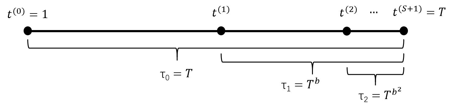
Refer to caption
Figure 6: The restart schedule of Algorithm 4
Algorithm 4 Primal-Dual Restart (𝖠𝖫𝖦𝟦\mathsf{ALG4})
1:  Input: time length τu\tau_{u}, parameters αu\alpha_{u}, βu\beta_{u}, γu\gamma_{u} for u=0,1,…,Su=0,1,\ldots,S.
2:  Initialize: set initial capacity C⁡(1)=CC(1)=C;
3:  for u=0,1,…,Su=0,1,\ldots,S do
4:    if u<Su<S then
5:    C(u)←C⁡(T−τu+1)C^{(u)}\leftarrow C(T-\tau_{u}+1), t1(u)←T−τu+1t_{1}^{(u)}\leftarrow T-\tau_{u}+1 and t2(u)←T−τu+1t_{2}^{(u)}\leftarrow T-\tau_{u+1}
6:    else
7:    C(u)←C⁡(T−τu+1)C^{(u)}\leftarrow C(T-\tau_{u}+1), t1(u)←T−τu+1t_{1}^{(u)}\leftarrow T-\tau_{u}+1 and t2(u)←Tt_{2}^{(u)}\leftarrow T
8:    end if
9:    Run Algorithm 3 subroutine which begins with t1(u)t_{1}^{(u)} and ends with t2(u)t_{2}^{(u)}. Let the initial capacity be C(u)C^{(u)}, let technical parameters be αu,βu,γu\alpha_{u},\beta_{u},\gamma_{u}.
10:  end for
Algorithm 5 LP-based Thresholding (𝖠𝖫𝖦𝟧\mathsf{ALG5})
1:  Input: start time t1t_{1}, end time t2t_{2}, initial capacity at start time BB;     parameter β\beta where β∈(0,12)\beta\in(0,\frac{1}{2}), parameter dd where d<(−β,β−12)d<(-\beta,\beta-\frac{1}{2})
2:  Initialize: set b=12+βb=\frac{1}{2}+\beta, set L=T−t1+1L=T-t_{1}+1, l1=⌈L−Lb⌉l_{1}=\lceil L-L^{b}\rceil, set B⁡(t1)=BB(t_{1})=B,
3:  calculate x∗=argmaxx{∑j∈[n]rjxj∣∑j=1nAjxj≤B⁡(t1)L,0≤xj≤λj,∀j∈[n]}x^{*}=\arg\max_{x}\left\{\sum_{j\in[n]}r_{j}x_{j}\mid\sum_{j=1}^{n}A_{j}x_{j}\leq\frac{B(t_{1})}{L},0\leq x_{j}\leq\lambda_{j},\,\forall\,j\in[n]\right\}.
4:  for j∈[n]j\in[n] do
5:    if xj∗<λj​Ldx^{*}_{j}<\lambda_{j}L^{d} then
6:    set pj←0p_{j}\leftarrow 0
7:    else if xj∗>λj​(1−Ld)x^{*}_{j}>\lambda_{j}(1-L^{d}) then
8:    set pj←1p_{j}\leftarrow 1
9:    else
10:    set pj←xj∗/λjp_{j}\leftarrow x_{j}^{*}/\lambda_{j}
11:    end if
12:  end for
13:  Phase I. Thresholding
14:  for t=t1,t1+1,…,t1+l1−1t=t_{1},t_{1}+1,\ldots,t_{1}+l_{1}-1 do
15:    Observe customer of type j⁡(t)j(t)
16:    if Aj≤B⁡(t)​∀j∈[n]A_{j}\leq B(t)\,\forall\,j\in[n] then
17:    Accept the customer with probability pj⁡(t)p_{j(t)};
18:    If accepted, update B⁡(t+1)←B⁡(t)−Aj⁡(t)B(t+1)\leftarrow B(t)-A_{j(t)}
19:    else
20:    Reject the customer
21:    end if
22:  end for
23:  Phase II. Run Algorithm 2 subroutine with start time t1+l1t_{1}+l_{1}, end time t2t_{2}, and initial capacity B⁡(t1+l1)B(t_{1}+l_{1}).
Algorithm 6 Hybrid Restart (𝖠𝖫𝖦𝟨\mathsf{ALG6})
1:  Input: time length τu\tau_{u} for u=0,1,…,Su=0,1,\ldots,S; (Algorithm 5 subroutine) parameters βu\beta_{u} and dud_{u} for u=0,1,…,Uu=0,1,\ldots,U; (Algorithm 3 subroutine) parameters αu\alpha_{u}, βu\beta_{u} and γu\gamma_{u} for u=U+1,…​Su=U+1,\ldots S.
2:  Initialize: set initial capacity C⁡(1)=CC(1)=C
3:  for u=0,1,…,Su=0,1,\ldots,S do
4:    if u<Su<S then
5:    C(u)←C⁡(T−τu+1)C^{(u)}\leftarrow C(T-\tau_{u}+1), t1(u)←T−τu+1t_{1}^{(u)}\leftarrow T-\tau_{u}+1 and t2(u)←T−τu+1t_{2}^{(u)}\leftarrow T-\tau_{u+1}
6:    else
7:    C(u)←C⁡(T−τu+1)C^{(u)}\leftarrow C(T-\tau_{u}+1), t1(u)←T−τu+1t_{1}^{(u)}\leftarrow T-\tau_{u}+1 and t2(u)←Tt_{2}^{(u)}\leftarrow T
8:    end if
9:    if u<Uu<U then
10:    Run Algorithm 5 with start time t1(u)t_{1}^{(u)}, end time t2(u)t_{2}^{(u)}, initial capacity C(u)C^{(u)} at start time, and parameters βu\beta_{u}, dud_{u}.
11:    else
12:    Run Algorithm 3 which begins with t1(u)t_{1}^{(u)} and ends with t2(u)t_{2}^{(u)}. Let the initial capacity be C(u)C^{(u)}, let technical parameters be αu,βu,γu\alpha_{u},\beta_{u},\gamma_{u}.
13:    end if
14:  end for

C.2 Hybrid restart algorithm

In the following, we first introduce the LP-based thresholding algorithm in Algorithm 5, which is called as subroutines in Algorithm 6.

Algorithm 5 takes as inputs a start time t1t_{1}, an end time t2t_{2}, initial capacity BB at the start time, and technical parameters β\beta and dd that satisfy β∈(0,12)\beta\in(0,\frac{1}{2}) and d<(−β,β−12)d<(-\beta,\beta-\frac{1}{2}).

At the beginning of the time horizon, Algorithm 5 solves a DLP, and uses its optimal solution to calculates the thresholding conditions. The entire horizon is then divided in two “phases”: in phase I, Algorithm 5 makes probabilistic allocation decisions; in phase II, Algorithm 5 runs the primal-dual algorithm in Algorithm 2.

Now we introduce Algorithm 6, which is a hybrid of Algorithm 5 and Algorithm 3 under a similar restart schedule shown in Figure 6.

Algorithm 6 includes a total of S+1S+1 epochs. Each epoch uu, where u=0,1,…,Su=0,1,\ldots,S, starts from period T−τu+1T-\tau_{u}+1 and ends at period T−τu+1T-\tau_{u+1}, where τu\tau_{u} is the time length between the starting period of epoch uu and period TT. At the beginning of the first UU epochs, Algorithm 6 runs (restarts) Algorithm 5 as a a subroutine, and at the beginning of the remaining S−U+1S-U+1 epochs, Algorithm 6 runs (restarts) Algorithm 3 as a subroutine.

More precisely, we design the restart schedule as follows: in the first UU epochs, Algorithm 6 only runs phase I of Algorithm 5; in the next S−US-U epochs, Algorithm 6 only runs phase I and phase II of Algorithm 3; and in the last epoch, Algorithm 6 runs all three phases of Algorithm 3.