Softly shifting away from dark matter direct detection
Abstract
We propose soft breaking mechanism for dark matter (DM) shift symmetry in a class of composite dark matter models, where both DM and the Higgs boson arise as pseudo Nambu-Goldstone bosons from novel strong dynamics. Our mechanism is utilized to suppress the non-derivative portal coupling between the Higgs boson and DM particle, which can evade the stringent bound of current DM direct detection experiments. Otherwise this non-derivative portal coupling would naturally be at the same order of the Higgs quartic, rendering this class of models under severe crisis. For realizing soft breaking mechanism, we introduce vector-like top partners, dubbed as “softons”, to restore the shift symmetry of DM in top Yukawa sector, which however is only broken by the softon masses. The portal coupling would automatically vanish as the shift-symmetry-breaking softon masses approach zero. Specifically we present a proof-of-concept model of soft breaking, based on the coset and the simplest fermion embedding, and study its DM phenomenology, where we show a large amount of novel parameter space is opened up by using the soft breaking mechanism.
I Introduction
One plausible resolution to the hierarchy problem is to consider the Higgs as a pseudo Nambu-Goldstone boson (PNGB) emerging from spontaneous global symmetry breaking of a new strongly-interacting sector. In this scenario, Higgs is protected by an approximate shift symmetry and thus naturally lighter than the typical scale of the strong sector. The minimal realization Agashe et al. 2005; Contino et al. 2007; Contino 2011 contains four Goldstone bosons forming the Higgs doublet. Electroweak symmetry breaking (EWSB) is triggered due to radiative corrections and the masses of the Higgs and EW gauge bosons are at the same scale. The mass scale of the strong sector resonances can be uplifted beyond current collider limits Blasi and Goertz 2019 and the scenario is still phenomenologically intriguing. Besides, extra Goldstones arise if non-minimal symmetry breaking patterns are employed Gripaios et al. 2009; Mrazek et al. 2011; Da Rold and Rossia 2019. Some of these Goldstones are natural dark matter (DM) candidates if they are stabilized by a discrete parity or dark symmetry Frigerio et al. 2012; Chala 2013; Marzocca and Urbano 2014; Fonseca et al. 2015; Balkin et al. 2017; Wu et al. 2017; Balkin et al. 2018; Davoli et al. 2019; Cacciapaglia et al. 2019; Ramos 2019; Ahmed et al. 2020, where the Higgs and DM are unified in the same framework with comparable masses and DM would exhibit typical phenomenology of weakly interacting massive particles (WIMP); see e.g. Bertone et al. 2005; Lisanti 2017; Bauer and Plehn 2019; Profumo et al. 2019 for reviews.
Within this class of models, when DM candidates are gauge singlets of the Standard Model (SM), they interact with SM particles mainly through the Higgs portal. The leading operators characterizing the portal interactions between the Higgs doublet and the real singlet scalar DM are Balkin et al. 2018
| (1) |
where denotes the symmetry breaking scale and is the coupling strength of the usual Higgs portal interaction. The operator characterizes the derivative portal coupling originating from the Goldstone nature of the Higgs and DM, while the operator only arises from the radiative scalar potential of the Goldstones. Phenomenologically, is enhanced in the high energy regime and dominates over , e.g. in DM annihilation, although has higher mass dimension. Nevertheless, would dominate in direct detection experiments, where is highly suppressed due to small momentum transfer Barducci et al. 2017. Therefore, direct detection experiments already impose stringent bound on the coupling strength . Following naive dimensional analysis (NDA), is estimated to be of the same order of the Higgs quartic as , if the top sector breaks both the shift symmetry of the Higgs and DM. However, this value of is in tension with current direct detection bounds Akerib et al. 2017; Cui et al. 2017; Aprile et al. 2018. Motivated by this fact, top sector is required to fully respect the DM shift symmetry, which usually renders the top sector non-minimal. Two different scenarios are proposed and discussed in Ref. Balkin et al. 2018 to evade direct detection bounds and can be automatically suppressed if the leading shift-symmetry breaking effects arise in the bottom sector rather than the top sector, or a novel dark photon sector with all the quarks preserving the DM shift symmetry.
In this work, we propose a mechanism for softly breaking the DM shift symmetry in the top sector, leading to suppressed portal coupling while DM still lives in the weak scale. In conventional top sectors, DM shift symmetry is broken since top quark does not fulfill complete representations of the global symmetry. In contrast, to realize soft-breaking, two model ingredients are as follows.
- 1.
Extra vector-like top partners, dubbed as “softons”, are introduced to restore exact DM shift symmetry in top Yukawa terms.
- 2.
Softon mass terms are naturally introduced, and they softly break DM shift symmetry, leading to nonzero DM mass and the portal coupling .
The numerical value of the portal coupling is proportional to the shift-symmetry-breaking softon masses. At the limit of zero softon masses, DM particle remains an exact Goldstone boson and all the non-derivative terms of DM vanish. For TeV-scale softon masses, can be small enough to evade the bounds of direct detection experiments. In parallel, we note that similar idea is implemented to eliminate quadratic divergence in neutral-naturalness models Xu et al. 2020 and stabilize the Higgs mass in composite Higgs models Blasi and Goertz 2019; Blasi et al. 2020. Also, in Ref. Ahmed et al. 2020, direct detection signal is reduced by giving vector-like masses to the symmetry partners of the top quark, in which these top partners are part of a neutral-naturalness construction. Here we will discusse the soft breaking mechanism in a more general framework, and demonstrate the idea in the top sector of a more minimal model.
II Soft Breaking Mechanism
As a proof-of-concept example, we focus on the next-to-minimal coset Gripaios et al. 2009 to illustrate the soft-breaking mechanism for PNGB DM, and similar implementation can straightforwardly be generalized to other cosets. In the following, we explain in details the implementation in the top sector.
Within the unbroken global symmetry, the custodial symmetry is identified as where is further weakly gauged. In the unitary gauge, the PNGBs are explicitly
| (2) |
transforming as a fundamental representation of global symmetry and satisfying the constraint . Within the field , is a DM candidate if it is stabilized by symmetries, and this is achieved by imposing a dark parity as , with which the global symmetry is enlarged to Frigerio et al. 2012. Under the parity , is odd while all the SM particles are even. All the terms that are odd under , including the Wess-Zumino-Witten terms Wess and Zumino 1971; Witten 1983; Chu et al. 1996, are forbidden. If is the lightest -odd particle, it is stable and serves as a good DM candidate.
DM mass and the non-derivative Higgs-DM portal coupling are induced by any explicit shift-symmetry breaking effects. Since is a SM singlet, SM gauge bosons do not break DM shift symmetry. Though, explicit breaking effects can generally arise in fermion sectors, especially the top sector, as SM fermions are embedded in incomplete representations of . For example, when the electroweak doublet and singlet are both embedded in fundamental representations of , respects the DM shift symmetry while breaks it. In order to fully restore DM shift symmetry in the top Yukawa sector, a vector-like softon field is introduced, where the right-handed component is embedded such that the Lagrangian is invariant under the rotation acting on the fifth and sixth components in accordance with the field as shown in Eq. 2:
| (3) |
and therefore is invariant, i.e.
| (4) |
where the fermionic fields are
| (5) |
This rotation defines the shift symmetry of , i.e. is an exact Goldstone boson if the rotation remains an unbroken symmetry. For any non-vanishing dependence of in the Yukawa sector, one can always perform an rotation to rotate it away. Furthermore, the left-handed component is assumed as a singlet. One can introduce the mass term of as
| (6) |
which breaks explicitly and serves as the only source that gives nonzero DM mass and portal coupling , rendering a PNGB.
In the momentum space, the effective Lagrangian below the scale of strong dynamics is
| (7) |
where are the momentum-dependent form factors which are all calculable in concrete composite models. In the decoupling limit of , one can turn off the fermionic field , this corresponds to the breaking of DM shift symmetry in conventional top sectors. Notice the terms and are forbidden as they are odd under the dark parity.
III Effective Potential
In the following, we present a concrete composite model from which one can match to the effective Lagrangian in Eq. 7 and calculate the scalar potential, where the leading terms are given by
| (8) |
In particular, we demonstrate that the portal coupling in the soft-breaking scenario is suppressed compared to its NDA value, which however can be recovered at the decoupling limit as .
We introduce composite resonances and arising from strong dynamics, which are respectively in the fundamental representation and singlet of , and construct the composite model following CCWZ Coleman et al. 1969; Callan et al. 1969 with the Goldstone matrix , where are the Goldstone bosons and are the broken generators of . Notice the Goldstone matrix realizes the symmetry nonlinearly. Under the paradigm of partial compositeness Kaplan 1991,
| (9) |
where , indicate the layers of composite resonances, and various ’s are the mixing parameters between the elementary fields and the composites . We consider the minimal scenario with only one layer of composites, i.e. in this work, which however is not viable in the models of hard shift symmetry breaking Marzocca and Urbano 2014. The top mass is obtained after integrating out heavy composites and turning on the Higgs vacuum expectation value, e.g. in Marzocca et al. 2012; Panico and Wulzer 2016.
As shown in Fig. 1, one consequence of imposing soft breaking is that the scalar does not suffer from the usual quadratic divergence. Because the dependence on vanishes in the quadratically divergent diagrams and , which do not have insertions. Once is inserted, e.g. as in , the diagrams with non-vanishing dependence of arise, and they are at most logarithmically divergent or finite. Notice we only consider the contribution coming from the composite in Fig. 1, likewise one can also include the contribution of the composite . Insertions of can further reduce the degree of divergence of the diagrams as shown in Fig. 1, however the terms of non-vanishing in the potential cannot arise without insertions.
In order to get rid of all the divergences and make the scalar potential fully calculable, one can impose Weinberg sum rules (WSRs) Marzocca et al. 2012; Pomarol and Riva 2012; Li et al. 2019. When , one optimal choice can be
| (10) |
with which we calculate the form factors in Eq. 7 and the scalar potential in Eq. 8. Other choices of WSRs only modify the quantitative range of viable parameter space of various masses and mixings in Eq. 9, if all the low energy parameters in the scalar potential and the top mass are fixed. But the overall qualitative relations of various parameters will not change. The portal coupling is now calculable. When the mixing is smaller than the symmetry breaking scale ,
| (11) |
where is the QCD color factor from the top sector. At the decoupling limit of , the conventional portal coupling at the NDA size Marzocca and Urbano 2014 is recovered, i.e.
| (12) |
In contrast, when , an suppression factor for , defined as the ratio of the portal coupling in the shift-symmetry-soft-breaking scenario and that in the hard-breaking scenario, is obtained as
| (13) |
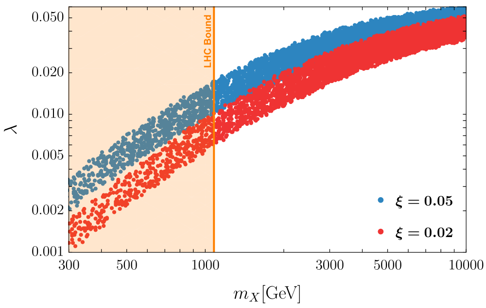
where denotes the overall mass scale of the strong dynamics, i.e. . The smaller the value of , the smaller the portal coupling . Without using the above approximation in the small limit, we scan the parameters in the composite model and plot the relation between and , as shown in Fig. 2. In the scan, we require the top mass, the Higgs mass, and the EW scale are reproduced. The parameter denotes the usual vacuum misalignment angle, where we choose and which are consistent with the bounds from precision measurements of various Higgs couplings Li et al. 2019. When the softon is heavy enough, the value of approaches to the NDA value as . When is moderately heavier than the Large Hadron Collider (LHC) bound Belyaev et al. 2018, can be much suppressed with respect to the NDA value. For example, can be as small as when . And the portal coupling will be more suppressed if the scale of strong dynamics (and the scale of ) is larger, as shown in Eq. 13. Since the softon does not break the shift symmetry of the Higgs boson, the usual Higgs mass and quartic are reproduced.
IV Dark Matter Phenomenology
Since the mass of is at the EW scale, it is expected to exhibit traditional WIMP phenomenology, whereas it cannot be detected in current direct detection experiments. The numerical results are given in Fig. 3, where the details are summarized as follows.
In the early Universe, the relic abundance of is obtained by the freeze-out of the dark matter self-annihilation process, i.e. pair annihilating to SM particles. As given by the Planck collaboration Aghanim et al. 2018, the relic abundance of is bounded as . In the calculation of DM abundance, we assume the usual radiation dominance during DM freeze out. The derivative couplings, e.g. the operator in Eq. 1, are dominant in the annihilation processes when is heavy. As a result, even with much suppressed portal coupling , the correct relic abundance can be reproduced Frigerio et al. 2012. The softon field has only minor impact on determining the abundance. After the composite resonances are integrated out, the effective Lagrangian as in Eq. 7 is obtained, which in particular contains the vertex , where the softon is required to be heavier than such that is stable, and the searches for colored top partners also implies is above TeV scale Belyaev et al. 2018. Due to the heaviness of , the annihilation channel induced by is suppressed, and the DM co-annihilation Griest and Seckel 1991 with can also be neglected. All the other processes changing the number density of are irrelevant. Consequently, the freeze-out of in the early universe is dominated by the self-annihilaiton process in the Higgs portal. The relic abundance of reads,
| (14) |
where and denotes the freeze-out temperature. is the quantity of the thermally averaged cross section of DM annihilation at the freeze-out temperature. In this model, we have Balkin et al. 2017,
| (15) |
where is the center-of-mass energy. The first term in the right-handed side of the equation is from operator while the second from operator . The minus sign in the brackets indicates the cancellation of these two operators. Thus, for dark matter with certain mass, there could be two different values of that correspond to correct relic abundance. This feature is shown explicitly in Fig. 3, where the observed DM abundance is denoted with the black bands.
As motivated in previous sections, is much suppressed and therefore the bounds from current direct detection experiments are evaded. The spin-independent (SI) DM-nucleon cross section induced by operator is given in Ref. Cline et al. 2013; Arcadi et al. 2019, which is the same as the usual Higgs portal singlet DM. To be specific, it is given by,
| (16) |
Here, we have and for Xenon, and is the average nucleon mass. describe the coupling between DM and the necleons. Substituting the values of these quantities, it reads,
| (17) |
Such a value of DM-nucleon cross section lies well below the bounds of current direct detection experiments. In addition, the softon only contributes to DM-nucleon scatterings at loop levels. When the tree-level DM-nucleon scatterings are suppressed due to the smallness of as in our model, one-loop DM-nucleon scatterings can possibly dominate over tree-level ones. The yellow-shaded region is excluded by the current Xenon-1T experiment Aprile et al. 2018, and the reach of future LZ experiment Akerib et al. 2020 is also shown by the yellow dashed line. For completeness, we also show the constraints from indirect detection experiments, where the results from Fermi-LAT collaboration Ackermann et al. 2015; Albert et al. 2017 are used and we require the total thermal-averaged DM annihilation cross section to be smaller then the value reported by Fermi-LAT, assuming all the DM particles annihilate to the final state. In Fig. 3, the blue-shaded region is excluded by the current bounds Ackermann et al. 2015; Albert et al. 2017 and the future projection Charles et al. 2016 is given by blue-dashed curve. Numerically, we note that the relic abundance of and direct/indirect detection bounds are computed with the help of the public code micrOMEGAs Bélanger et al. 2018 and the model files are obatined with FeynRules Alloul et al. 2014. The constraints on DM mass and portal coupling from invisible Higgs decay is not included here since we concentrate on the heacy DM region with .
In addition, we present the result from parameter scan, as shown by the dots in Fig. 3. We scanned randomly within the parameter range of . is a parameter from the gauge sector Marzocca and Urbano 2014. Meanwhile, we require all the heavy resonances lie above the current LHC bounds, e.g. Aaboud et al. 2018; Sirunyan et al. 2019; Belyaev et al. 2018; Liu et al. 2019, and the correct Higgs and top masses, as well as the electroweak scale are reproduced. The dots that do not meet these requisites are abandoned and not shown. As is seen in Fig. 3, only the unshaded red dots are fully viable under the current bounds from direct detection (yellow region), indirect detection (blue region), and relic abundance (black). All the other dots in the shaded region are excluded for various reasons, and the green dots indicate the region where DM are over produced. In particular, compared to the NDA-size portal coupling in Marzocca and Urbano 2014 as shown by the pink band, the portal coupling in our model is much suppressed, and a large amount of viable parameter space, as represented by the unshaded red dots, is opened up, which can be tested in the near future.
V Concluding Remarks
We propose soft-breaking mechanism for the shift symmetry of PNGB DM, which is still at the EW scale whereas the stringent bounds from current direct detection are evaded. We present a proof-of-concept model to demonstrate the usefulness of our mechanism. Generalizations to other models are straightforward. In addition, we notice that the similar soft-breaking mechanism can also be implemented to break the Higgs shift symmetry Blasi and Goertz 2019, where the top partner masses can be uplifted. Implementing the soft breaking for both the Higgs and DM shift symmetries would lead to “double” suppression for the non-derivative portal coupling, i.e.
| (18) |
where is the typical scale of strong dynamics, and are the softon masses for the breaking of the DM and Higgs shift symmetries, respectively. When the portal coupling is very suppressed, one-loop DM-nucleon scatterings will dominate over the tree-level ones in this class of models. We leave this for future investigation.
Acknowledgments
L.X.X. would like to thank Roberto Contino, Rashmish K. Mishra, Alessandro Podo for valuable discussions on related topics, and Scuola Normale for warm hospitality when working on this project. This work is supported in part by the National Science Foundation of China under Grants No. 11635001, 11875072.
Appendix A From CCWZ Construction to Effective Potential
Generators for group are chosen as follows,
where counts broken generators, while count generators of the subgroup and counts others. There are five Goldstones corresponding to five broken generators. Four of them living in fundamental representation of are identified as Higgs doublet and the other one which is singlet is considered as dark matter candidate. These Goldstone bosons can be parameterized by . We use to represent the Goldstone bosons here. It is convenient to perform a field redefinition Gripaios et al. 2009 in the calculation: , where . To build Lagrangian, it is necessary to define CCWZ symbols and ,
is covariant derivative if a subgroup of is gauged. In our case, the gauged subgroup is the electroweak gauge group . We used to count all unbroken generators of . With the exception of the Wess-Zumino-Witten term Wess and Zumino 1971; Witten 1983; Chu et al. 1996, all terms can be constructed with and symbols. In leading order, we have,
Expanding this term, we can deduce the Lagrangian of Goldstones and .
For spin-1 resonances, we denote the resonances as (adjoint representation) and (fundamental representation). The Lagrangian is
denote the decay constants for and respectively, and and are constants. The field strengths and covariant derivatives are defined as
Note that mass terms in contain mixing terms between spin-1 resonances and electroweak gauge fields. Integrating these heavy resonances out, we will get effective Lagrangian for electroweak gauge bosons. In momentum space,
| (19) |
where,
are electroweak gauge coupling constants. In Euclidean space, the form factors are
Consequently, contribution to effective potential from the gauge sector reads
| (20) |
is -independent since is singlet of electroweak gauge group. To render the integral finite, we need WSRs to eliminate divergence.
| (21) |
In parameter scan, we will use and as free parameters and deduce and accordingly with these two WSRs.
For fermion contribution, we add the expressions of the form factors in Eq. 7 here,
| (22) |
The scalar potential can be deduced from Eq. 7 and the coefficients in Eq. 8 are integrals of the form factors.
| (23) | ||||
We defined . To eliminate quadratic divergence in , we need to impose the following WSRs,
The cancellation of logarithmic divergence in requires,
Once these conditions are satisfied, all the UV divergences in the integrals Eq. A disappear. In the case of that is adopted in this work, one appropriate choice of WSRs that accomodates experimental constraints better is
where is a constant. Note that is also IR divergent. It’s because effective potential is singular at . This issue can be cured by introducing another term Marzocca et al. 2014. It absorbs the singularity of Higgs quartic coupling constant. Nevertheless, we will simply cutoff this divergence with .
References
- Agashe et al. (2005) K. Agashe, R. Contino, and A. Pomarol, Nucl. Phys. B719, 165 (2005), arXiv:hep-ph/0412089 [hep-ph] .
- Contino et al. (2007) R. Contino, L. Da Rold, and A. Pomarol, Phys. Rev. D75, 055014 (2007), arXiv:hep-ph/0612048 [hep-ph] .
- Contino (2011) R. Contino, in Physics of the large and the small, TASI 09, proceedings of the Theoretical Advanced Study Institute in Elementary Particle Physics, Boulder, Colorado, USA, 1-26 June 2009 (2011) pp. 235–306, arXiv:1005.4269 [hep-ph] .
- Blasi and Goertz (2019) S. Blasi and F. Goertz, Phys. Rev. Lett. 123, 221801 (2019), arXiv:1903.06146 [hep-ph] .
- Gripaios et al. (2009) B. Gripaios, A. Pomarol, F. Riva, and J. Serra, JHEP 04, 070 (2009), arXiv:0902.1483 [hep-ph] .
- Mrazek et al. (2011) J. Mrazek, A. Pomarol, R. Rattazzi, M. Redi, J. Serra, and A. Wulzer, Nucl. Phys. B 853, 1 (2011), arXiv:1105.5403 [hep-ph] .
- Da Rold and Rossia (2019) L. Da Rold and A. N. Rossia, JHEP 12, 023 (2019), arXiv:1904.02560 [hep-ph] .
- Frigerio et al. (2012) M. Frigerio, A. Pomarol, F. Riva, and A. Urbano, JHEP 07, 015 (2012), arXiv:1204.2808 [hep-ph] .
- Chala (2013) M. Chala, JHEP 01, 122 (2013), arXiv:1210.6208 [hep-ph] .
- Marzocca and Urbano (2014) D. Marzocca and A. Urbano, JHEP 07, 107 (2014), arXiv:1404.7419 [hep-ph] .
- Fonseca et al. (2015) N. Fonseca, R. Zukanovich Funchal, A. Lessa, and L. Lopez-Honorez, JHEP 06, 154 (2015), arXiv:1501.05957 [hep-ph] .
- Balkin et al. (2017) R. Balkin, M. Ruhdorfer, E. Salvioni, and A. Weiler, JHEP 11, 094 (2017), arXiv:1707.07685 [hep-ph] .
- Wu et al. (2017) Y. Wu, T. Ma, B. Zhang, and G. Cacciapaglia, JHEP 11, 058 (2017), arXiv:1703.06903 [hep-ph] .
- Balkin et al. (2018) R. Balkin, M. Ruhdorfer, E. Salvioni, and A. Weiler, JCAP 1811, 050 (2018), arXiv:1809.09106 [hep-ph] .
- Davoli et al. (2019) A. Davoli, A. De Simone, D. Marzocca, and A. Morandini, JHEP 10, 196 (2019), arXiv:1905.13244 [hep-ph] .
- Cacciapaglia et al. (2019) G. Cacciapaglia, H. Cai, A. Deandrea, and A. Kushwaha, JHEP 10, 035 (2019), arXiv:1904.09301 [hep-ph] .
- Ramos (2019) M. Ramos, (2019), arXiv:1912.11061 [hep-ph] .
- Ahmed et al. (2020) A. Ahmed, S. Najjari, and C. B. Verhaaren, (2020), arXiv:2003.08947 [hep-ph] .
- Bertone et al. (2005) G. Bertone, D. Hooper, and J. Silk, Phys. Rept. 405, 279 (2005), arXiv:hep-ph/0404175 .
- Lisanti (2017) M. Lisanti, in Proceedings, Theoretical Advanced Study Institute in Elementary Particle Physics: New Frontiers in Fields and Strings (TASI 2015): Boulder, CO, USA, June 1-26, 2015 (2017) pp. 399–446, arXiv:1603.03797 [hep-ph] .
- Bauer and Plehn (2019) M. Bauer and T. Plehn, Lect. Notes Phys. 959, pp. (2019), arXiv:1705.01987 [hep-ph] .
- Profumo et al. (2019) S. Profumo, L. Giani, and O. F. Piattella, Universe 5, 213 (2019), arXiv:1910.05610 [hep-ph] .
- Barducci et al. (2017) D. Barducci, A. Bharucha, N. Desai, M. Frigerio, B. Fuks, A. Goudelis, S. Kulkarni, G. Polesello, and D. Sengupta, JHEP 01, 078 (2017), arXiv:1609.07490 [hep-ph] .
- Akerib et al. (2017) D. S. Akerib et al. (LUX), Phys. Rev. Lett. 118, 021303 (2017), arXiv:1608.07648 [astro-ph.CO] .
- Cui et al. (2017) X. Cui et al. (PandaX-II), Phys. Rev. Lett. 119, 181302 (2017), arXiv:1708.06917 [astro-ph.CO] .
- Aprile et al. (2018) E. Aprile et al. (XENON), Phys. Rev. Lett. 121, 111302 (2018), arXiv:1805.12562 [astro-ph.CO] .
- Xu et al. (2020) L.-X. Xu, J.-H. Yu, and S.-H. Zhu, Phys. Rev. D 101, 095014 (2020), arXiv:1810.01882 [hep-ph] .
- Blasi et al. (2020) S. Blasi, C. Csaki, and F. Goertz, (2020), arXiv:2004.06120 [hep-ph] .
- Wess and Zumino (1971) J. Wess and B. Zumino, Phys. Lett. 37B, 95 (1971).
- Witten (1983) E. Witten, Nucl. Phys. B223, 422 (1983).
- Chu et al. (1996) C.-S. Chu, P.-M. Ho, and B. Zumino, Nucl. Phys. B475, 484 (1996), arXiv:hep-th/9602093 [hep-th] .
- Coleman et al. (1969) S. R. Coleman, J. Wess, and B. Zumino, Phys. Rev. 177, 2239 (1969).
- Callan et al. (1969) C. G. Callan, Jr., S. R. Coleman, J. Wess, and B. Zumino, Phys. Rev. 177, 2247 (1969).
- Kaplan (1991) D. B. Kaplan, Nucl. Phys. B365, 259 (1991).
- Marzocca et al. (2012) D. Marzocca, M. Serone, and J. Shu, JHEP 08, 013 (2012), arXiv:1205.0770 [hep-ph] .
- Panico and Wulzer (2016) G. Panico and A. Wulzer, Lect. Notes Phys. 913, pp.1 (2016), arXiv:1506.01961 [hep-ph] .
- Pomarol and Riva (2012) A. Pomarol and F. Riva, JHEP 08, 135 (2012), arXiv:1205.6434 [hep-ph] .
- Li et al. (2019) H.-L. Li, L.-X. Xu, J.-H. Yu, and S.-H. Zhu, JHEP 09, 010 (2019), arXiv:1904.05359 [hep-ph] .
- Belyaev et al. (2018) A. S. Belyaev, T. Flacke, B. Jain, and P. B. Schaefers, Phys. Rev. D98, 035019 (2018), arXiv:1707.07000 [hep-ph] .
- Aghanim et al. (2018) N. Aghanim et al. (Planck), (2018), arXiv:1807.06209 [astro-ph.CO] .
- Griest and Seckel (1991) K. Griest and D. Seckel, Phys. Rev. D 43, 3191 (1991).
- Cline et al. (2013) J. M. Cline, K. Kainulainen, P. Scott, and C. Weniger, Phys. Rev. D88, 055025 (2013), [Erratum: Phys. Rev.D92,no.3,039906(2015)], arXiv:1306.4710 [hep-ph] .
- Arcadi et al. (2019) G. Arcadi, A. Djouadi, and M. Raidal, (2019), arXiv:1903.03616 [hep-ph] .
- Akerib et al. (2020) D. Akerib et al. (LUX-ZEPLIN), Phys. Rev. D 101, 052002 (2020), arXiv:1802.06039 [astro-ph.IM] .
- Ackermann et al. (2015) M. Ackermann et al. (Fermi-LAT), Phys. Rev. Lett. 115, 231301 (2015), arXiv:1503.02641 [astro-ph.HE] .
- Albert et al. (2017) A. Albert et al. (Fermi-LAT, DES), Astrophys. J. 834, 110 (2017), arXiv:1611.03184 [astro-ph.HE] .
- Charles et al. (2016) E. Charles et al. (Fermi-LAT), Phys. Rept. 636, 1 (2016), arXiv:1605.02016 [astro-ph.HE] .
- Bélanger et al. (2018) G. Bélanger, F. Boudjema, A. Goudelis, A. Pukhov, and B. Zaldivar, Comput. Phys. Commun. 231, 173 (2018), arXiv:1801.03509 [hep-ph] .
- Alloul et al. (2014) A. Alloul, N. D. Christensen, C. Degrande, C. Duhr, and B. Fuks, Comput. Phys. Commun. 185, 2250 (2014), arXiv:1310.1921 [hep-ph] .
- Aaboud et al. (2018) M. Aaboud et al. (ATLAS), Phys. Rev. Lett. 121, 211801 (2018), arXiv:1808.02343 [hep-ex] .
- Sirunyan et al. (2019) A. M. Sirunyan et al. (CMS), JHEP 03, 082 (2019), arXiv:1810.03188 [hep-ex] .
- Liu et al. (2019) D. Liu, L.-T. Wang, and K.-P. Xie, JHEP 01, 157 (2019), arXiv:1810.08954 [hep-ph] .
- Marzocca et al. (2014) D. Marzocca, A. Parolini, and M. Serone, JHEP 03, 099 (2014), arXiv:1312.5664 [hep-ph] .