Longitudinal data is usually collected by repeatedly observing the results for each subject at several points in time. It has been widely used in medical and economic research over the past decade. High-dimensional longitudinal data consisting of repeated measurements with a large number of covariates has become increasingly common in practical application. The number of covariates can be quite large, especially when the interactions of various factors are considered. Nevertheless, there is only a subset of covariates related to the response variables, and the redundant variables can affect the accuracy and efficiency of estimation. Therefore, it is important to develop a new methodology to select the important variables in high-dimensional longitudinal data.

To select the important variables in longitudinal data analysis, Pan, 2001 proposed a quasi-likelihood information criterion (QIC) based on an independence assumption, which can be used to select variables and working correlation matrices. Wang and Qu, 2009 combined the Bayesian information criterion with quadratic inference function, which does not require the full likelihood or quasi-likelihood. However, these two methods can be computationally intensive when the dimension of covariates $p$ is large. Tian et al., 2014 extended the SCAD-penalized quadratic inference function to analyze semiparametric varying coefficient partially linear models. Their proposed procedure simultaneously selects significant variables in the parametric components and the nonparametric components. Li et al., 2013 proposed an automatic variable selection procedure using smooth-threshold generalized estimating equations, which are based on the generalized estimating equations (GEE). Most of the above-mentioned methods only focused on the fixed dimension $p$. Thus, Wang et al., 2012 proposed a penalized GEE using a SCAD penalty and proved the asymptotic properties under the framework of large sample size $n$ and diverging $p$. The important feature of their method is that the consistency of model selection holds even if the working correlation structure is misspecified. However, the methods mentioned above are all based on the GEE. When the longitudinal data are contaminated or follow a heavy-tailed distribution, these methods are sensitive to response and/or covariates outliers. For example, in a large-scale yeast cell gene expression study reported by Spellman et al., 1998, genome-wide mRNA levels for $6178$ yeast open reading frames that can determine which amino acids will be encoded by a gene were recorded. The yeast cell cycle gene expression data cover approximately two cell-cycle periods and were collected at 7-minute intervals for 119 minutes, for a total of 18-time points measured at M/G1-G1-S-G2-M stages. Figure 1 reveals that there exist strong correlations and the correlation matrix is never a commonly used exchangeable or autoregressive matrix. Furthermore, apart from the strong correlations, we find that there are some outliers in the gene expression data (see Figure 2). Figure 3 indicates that abundant influence points occur in the observations of some important transcription factors, such as ASH1, MBP1, SWI4, and SWI6, which may lead to biased estimation and prediction. Some researchers have proposed various methods to identify important transcription factors (TFs) from a large set of transcription factors that are associated with gene expression levels and capture a complex relationship among those factors (Luan et al., 2003; Wang et al., 2007; Wang et al., 2012). Nevertheless, few researches focus on the robustness against outliers on observations and most of them fail to capture the underlying correlation structure within gene expression level on multiple observations.

Robust methods are desirable for contaminated data. Therefore, Fan et al., 2012 proposed robust penalized estimating equations based on Huber’s function for linear regression with longitudinal data, which is robust against outliers in response, but is sensitive to outliers in covariates. The regulated parameter in Huber’s function is directly specified. Lv et al., 2015 explored a weighted variable selection method based on an exponential squared loss (Wang et al., 2013) and a commonly used working correlation matrix for high dimensional longitudinal data, and they also provided a data-driven method to select the parameter in the exponential squared loss. These two methods are robust, but their work only looked at a specific case in which the variable dimension was no larger than the sample size, that is $p<n$.

In this article, we construct robust weighted estimating functions based on Tukey’s biweight score equations, which are robust for outliers in response and/ or covariates. Different from Li et al., 2013 using robust residuals to estimate the correlation parameter, we propose a novel robust working correlation matrix to capture the correlations, which is more close to the true correlation matrix than the exchangeable and AR(1) correlation matrices, and performs competitively with the true correlation structure in variable selection. Following Li et al., 2013 and Chang et al., 2018, we establish robust smooth-threshold estimating equations for parameter estimation and variable selection. Furthermore, we prove the asymptotic properties of the proposed method under “large $n$ and diverging $p$” setting. Robust estimating equations using bounded scores and leverage-based weights are robust against outliers and can reduce the bias when errors follow a heavy-tailed distribution. The proposed method can be applied to sparse marginal models under the large $n$ small $p$, large $n$ diverging $p$, and small $n$ large $p$.

The rest of the article is organized as follows: In Section 2.1, we construct a robust estimating equation (RTGEE) for parameter estimation and variable selection. In Section 2.2, we apply an iterative algorithm to solve the smooth-threshold generalized estimating equations. In Section 2.3, we establish an effective criterion for tuning parameter selection. In Section 3, we establish the oracle properties of the proposed method. In Section 4, we carry out extensive simulation studies to evaluate the performance of the proposed method. In Section 5, we analyze a yeast cell cycle dataset to illustrate the proposed method. Finally, in Section 6, we draw some conclusions.

Suppose that $Y_{i}=(y_{i1},\ldots,y_{im_{i}})^{\rm T}$ are measurements collected at times $(t_{i1},\ldots,t_{im_{i}})$ for the $i$th subject, where $i=1,\ldots,n$. Let $X_{i}=(x_{i1},\ldots,x_{im_{i}})$ be the corresponding covariate vector, in which $x_{ij}=(x_{ij1},\ldots,x_{ijp})^{\rm T}$ is a $p\times 1$ vector. Assume that observations from the same subject are correlated, and observations from different subjects are independent. Denote the marginal mean of $y_{ij}$ by $\mu_{ij}=E\left(y_{ij}|{x}_{ij}\right)=g\left(x_{ij}^{\top}\boldsymbol{\beta}\right)$, where $g(\cdot)$ is the inverse of the known link function, $\boldsymbol{\beta}=(\beta_{1},\ldots,\beta_{p})^{\rm T}$ is an unknown parameter vector, and variance of $y_{ij}$ is $\operatorname{Var}\left(y_{ij}|x_{ij}\right)=\phi v\left(\mu_{ij}\right)$ with a variance function $v(\cdot)$ and a scale parameter $\phi$. Let $\mu_{i}=(\mu_{i1},\ldots,\mu_{im_{i}})^{\rm T}$ and ${A}_{i}=\phi\operatorname{diag}\left(v\left(\mu_{i1}\right),\ldots,v\left(\mu_{im_{i}}\right)\right)$ be a diagonal matrix. The covariance matrix of $Y_{i}$ is ${Cov(Y_{i})}={A_{i}}^{1/2}{R_{T}}{A_{i}}^{1/2}$, where $R_{T}$ is the true correlation matrix of $Y_{i}$.

In this section, we will establish large sample properties of the proposed estimator under a “large $n$, diverging $p$” framework, which allows $p_{n}$ to diverge to $\infty$ as $n$ increases. The detailed proof of following Propositions are presented in the Appendix 1 in the Supplementary Information.

Let $\boldsymbol{\beta}_{0}=(\beta_{01},\ldots,\beta_{0p_{n}})^{\rm T}$ be the true value of $\boldsymbol{\beta}$, where $\boldsymbol{\beta}\in\mathbf{\Theta},\mathbf{\Theta}\subseteq\mathbb{R}^{p_{n}}$ is a bounded $p_{n}$-dimensional vector. Without loss of generality, we denote $\boldsymbol{\beta}_{0}=\left(\boldsymbol{\beta}_{01}^{T},\boldsymbol{\beta}_{02}^{T}\right)^{T}$, where $\boldsymbol{\beta}_{02}=\mathbf{0}$, and the elements of $\boldsymbol{\beta}_{01}$ are assumed to be nonzero in the dimension of $s_{n}$, which can also diverge with $n$. We partition $\boldsymbol{\beta}_{0}$ into active (nonzero) coefficient sets $\mathscr{A}_{0}=\left\{j:\beta_{0j}\neq 0\right\}$ with $|\mathscr{A}_{0}|=s_{n}$ and inactive (zero) coefficient sets $\mathscr{A}_{0}^{c}=\left\{j:\beta_{0j}=0\right\}$. We define the active set $\mathscr{A}=\left\{j:\hat{\delta}_{j}\neq 1\right\}$ as the set of indices of nonzero estimated coefficients. Under the following conditions, we present the consistency of the proposed estimator.

C1. Assume $x_{ij}$ for $1\leqslant i\leqslant n$ and $1\leqslant j\leqslant m_{i}$ satisfy $\sup_{i,j}\left\|x_{ij}\right\|=O\left(\sqrt{p_{n}}\right)$.

C2. The unknown parameter $\boldsymbol{\beta}$ belongs to a compact subset $\mathbf{\Theta}\subseteq\mathbb{R}^{p_{n}}$, and the true parameter value $\boldsymbol{\beta}_{0}$ lies in the interior of $\mathbf{\Theta}$. Furthermore, we assume that the estimator of the correlation parameter vector $\hat{\alpha}$ is $\sqrt{p_{n}/n}$-consistent given $\boldsymbol{\beta}$ and $\phi$ for some $\alpha$, that is, $\left\|\hat{\alpha}-\alpha\right\|=O_{p}\left(\sqrt{p_{n}/n}\right)$, and $|\partial\hat{\alpha}(\boldsymbol{\beta},\phi)/\partial\phi|\leq H({Y},\boldsymbol{\beta})$, where $H(\cdot,\cdot)$ is a bounded function for samples $Y$ and $\boldsymbol{\beta}$.

C3. Denote $\mathbf{X}_{i}^{h,b}=\mathbf{X}_{i}^{T}h_{0,i}^{b}\left({e}_{i}\right)$. There exists finite positive constants $c_{1}\leq c_{2}$ such that $\forall 1\leq j\leq m_{i}$:

where $h_{0,i}^{b}\left({e}_{i}\right)$ centers ${Y}_{i}$ by its true mean ${\mu}_{0,i}$ with ${\mu}_{0,i}={\mu}_{i}(\boldsymbol{\beta}_{0})$.

C4. $\sup_{i\geq 1}E\left\|h_{0,i}^{b}\left({e}_{i}\right)\right\|^{2+\delta}<\infty$ for some $\delta>0$, and $0<\sup_{i}\|Eh_{0,i}^{b}\left({e}_{i}\right)\left({h}_{0,i}^{b}\left({e}_{i}\right)\right)^{T}\|<\infty$, where ${h}_{i}^{b}\left({e}_{i}\right)$ centers by ${\mu}_{i}={\mu}_{i}(\boldsymbol{\beta})$.

C5. There exists a positive constant $c$ such that $0<c\leq\inf_{i,j}v\left(\mu_{ij}\right)\leq\sup_{i,j}v\left(\mu_{ij}\right)<\infty$. The functions $C_{ij}\left(\mu_{ij}\right)=E\left[\psi_{b}\left(A_{ij}^{-1/2}\left(y_{ij}-\mu_{ij}\right)\right)\right]$, $v(\cdot)$ and $g(\cdot)$ have bounded second derivatives. The function $\psi_{b}(\cdot)$ is piecewise twice differentiable, and the second derivatives are bounded.

C6. Assume that $E\left\|U_{n}\left(\boldsymbol{\beta}_{0}\right)\right\|^{2}<\infty$ and there exists $\delta>0$ such that

C7. Matrix

is positive definite. Matrix

is also positive definite.

C8. For any positive $\lambda$, $\tau$, $p_{n}$, and $s_{n}$, ${(p_{n}/n)}^{(1+\tau)/2}{\lambda}^{-1}\rightarrow 0$, $n^{-1/2}{\lambda}^{2}=o(1)$, and $s_{n}n^{-1/2}=o(1)$, such as $s_{n}=O(n^{1/3})$.

Remark Condition C1 is a common assumption in the M-estimator with diverging dimension (Portnoy, 1985), and it holds almost surely under some weak moment conditions for $x_{ij}$ from spherically symmetric distributions. Condition C2 is established to ensure the $\sqrt{p_{n}/n}$-consistency of $\hat{R}_{i}(\alpha)$ in Section 2.1, which can be verified using similar analysis in He et al., 2005. Taking the spirit of Lemma 3.7 in Wang, 2011, we set condition C3, which is especially useful when establishing the asymptotic normality in Proposition 2. Similar to Lv et al., 2015, conditions C4–C5 can be easily checked under bounded score function $\psi_{b}(\cdot)$, and they are usually combined with assumptions C6–C7, which are also necessary for the central limit theory and hold in most cases. Condition C8 is established for exploring convergence rate and asymptotic properties, which controls the order of diverging number $p_{n}$ and $s_{n}$ precisely, and we point out a series theoretical values for regularization parameter $\lambda$. Note that a preliminary $\sqrt{p_{n}/n}$-consistent estimator $\boldsymbol{\beta}_{0}$ is needed in both Proposition 1 and Proposition 2, which can be obtained by solving the generalized estimating equations under independent working correlation structure as in Example 1 in Wang, 2011 when $p_{n}\rightarrow\infty$.

Proposition 1 Suppose the regularity conditions C1–C8 hold, then we have

Proposition 2 Under conditions C1–C8, and if $n^{-1}p_{n}^{3}=o(1)$, as $n\rightarrow\infty$, we have
(1) variable selection consistency, $P\left(\mathscr{A}=\mathscr{A}_{0}\right)\rightarrow 1$;
(2) asymptotic normality: $\forall\boldsymbol{\alpha}_{n}\in R^{s_{n}}$ such that $\left\|\boldsymbol{\alpha}_{n}\right\|=1$,

where $\boldsymbol{\Sigma}_{\mathscr{A}_{0}}$ and $\mathbf{B}_{\mathscr{A}_{0}}$ are the first $s_{n}\times s_{n}$ submatrices of $\boldsymbol{\Sigma}$ and $\boldsymbol{B}$.

Proposition 1 implies that our proposed estimator can achieve $\sqrt{p_{n}/n}$-consistency. Proposition 2 shows that such consistent estimators possess the sparsity property and oracle property (Fan and Li, 2001) when we choose proper $\lambda$ and $\tau$. With a probability approaching 1, our proposed method can correctly select the nonzero coefficients and estimate them as efficiently as if we know the correct submodel in advance.

We conduct simulation studies to assess the performance of the proposed RTGEE method, the smooth-threshold generalized estimating equation (SGEE) proposed by Li et al., 2013, the robust smooth-threshold generalized estimating equation (RSGEE) corresponding to Huber’s score function, and the efficient and robust generalized estimating equation (ERSGEE) proposed by Lv et al., 2015 for continuous normal data and heavy-tailed data under setups $p<n$, large $n$ and diverging $p$, and $p>n$.

For each procedure, the true correlation structure of the response is exchangeable (EXC) with the correlation coefficient $\alpha=0.7$. For each setup in the simulations, we generate $100$ datasets and apply the iterative algorithm mentioned in Section 2.2 to estimate $\boldsymbol{\beta}$ and select important variables at the same time. Furthermore, we also consider the situation in which the true correlation structure is AR(1) with correlation parameter $\alpha=0.7$ for the continuous data. The simulation results show similar patterns and are presented in Tables 1–6 in the supplementary materials. Finally, we also consider the count data, and the results are listed in Tables 7–8 in the supplementary materials.

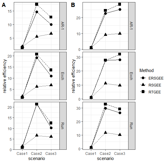
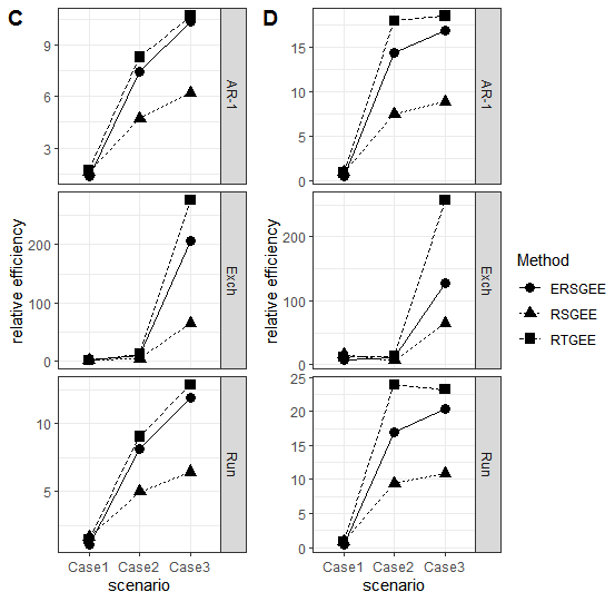
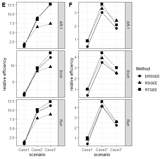
We compare these four methods under three working correlation matrices (EXC, AR(1), $R_{un}$) according to the following terms: the average number of correctly identified insignificant variables (C), the average number of incorrectly identified significant variables (IC), the correctly fitted odds (CF, the odd of identifying both significant variables and insignificant variables correctly over 100 simulations), the biases of estimators, the standard deviance (SD) of estimators, the proportion of estimators fall into the 95% confidence interval (CI), the average of mean squared prediction error (AMSPE), the median of mean squared prediction error (MMSPE), where $\text{MSPE}=n^{-1}\sum_{i=1}^{n}\left(\hat{y}_{i}-y_{i}\right)^{2}$, and the average mean square error (AMSE), which is the average of $\left\|\hat{\beta}-\beta_{0}\right\|^{2}$ over 100 simulations. To demonstrate the efficiency of estimators, we compare the relative efficiency among three robust methods in Figures 4–6, which is defined as the ratio of the AMSE for SGEE to the AMSE for each robust method, from which a higher value represents higher efficiency. We present partial results in Tables 1–6 and more details can be found in Tables 9–14 in Appendix 2 in the supplementary information.

The cell cycle is one of the most important processes for cell growth, DNA replication, chromosome segregation, and daughter cells’ division. Investigating the functions of gene expression during the cell cycle process can give an insight into how the cell cycle affects biological processes and cell cycle regulation. Transcription factors (TFs) are a critical part of the cell cycle process, where they have been shown to influence gene expression by regulating the flow of genetic information from DNA to mRNA during the cell cycle process. We are interested in selecting important TFs from a large set of candidates that are associated with yeast gene expression levels.

We apply the proposed RTGEE method to analyze the yeast cell cycle gene expression dataset, which was mentioned in Section 1. Our investigation indicates that log-transformed gene expression levels and observations of TFs contain many underlying outliers, thus it is worthwhile to reanalyze the yeast cell cycle via robust procedures. In this section, we apply SGEE, RSGEE, ERSGEE, and RTGEE to the dataset of the G1 stage in a yeast cell cycle with $1132$ observations ($283$ cell-cycled-regularized genes observed over 4-time points). The dataset is available in R package PGEE.

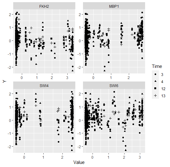
The scatter plot in Figure 7 depicts the complicated functional relationship among gene expression level and TFs, which is highly dependent on varying time, hence we consider following model, which is the same as Wang et al., 2012,

where the response variable $y_{ij}$ is the log-transformed gene expression level of gene $i$ measured at time point $j$, the covariates $x_{ik}$ are the matching score of the binding probability of the $k$th transcription factor on the promoter region of the $i$th gene for $k=1,\ldots,96$, and $t_{ij}$ represents the time points. We consider three correlation structures: EXC, AR(1), and $R_{un}$ for $\epsilon_{ij}$. Table 7 summarizes the selected numbers of TFs and the mean squared error for cross validation procedures ($\mathrm{MSE}_{\mathrm{CV}}$) to assess the goodness of fit:

where $\hat{\beta}_{(-i)}$ is the estimator obtained based on the data excluding the $i$th subject. The parameter estimates of the selected TFs are also given in Table 7.

The results indicate that the robust methods (RSGEE, ERSGEE, and RTGEE) select 25 TFs, while non-robust method (SGEE) select more TFs, from which, we find that significant TFs such as MBP1, SWI4, and SWI6 are selected by both robust and non-robust methods, which have been reported to function during the G1 stage in Simon et al., 2001. In addition, TFs such as FKH2, GAT3, GCR2, NDD1, SRD1, STB1 are commonly selected by all of the methods, and they are also confirmed in Wang et al., 2012. ABF1 is selected by SGEE in Wang et al., 2012, but not by the robust methods. Nevertheless, the transcription factor YAP5 noted as an important factor in Banerjee and Zhang, 2003 is consistently selected by all of the methods considered in our research, but not selected by Wang et al., 2012. Similarly, TFs such as MET31 and GCR1 selected by our robust methods have been verified in Tsai et al., 2005 and Song et al., 2014 respectively, while not been found in Wang et al., 2012.

In particular, Table 7 presents the mean squared error ($\text{MSE}_{\text{C V}}$) and also gives the running time of procedures. For this dataset analysis, our proposed method, RTGEE, performs better than other robust methods with the lower mean squared error under EXC and AR(1), and ERSGEE performs better than RSGEE. All of the methods using $R_{un}$ can be more competitive than other working correlation structures, though it can be more time-consuming. The longer running time of ERSGEE and our procedure RTGEE than other methods is associated with the fact that a wide range of tuning parameters is considered as in Section 2.3. To the best of our experience over abundant simulations, we recommend $b=7.0414$ for RTGEE in this yeast data analysis, which can also lead to a sufficient variable selection while saving a lot of time.

This article develops a robust automatic variable selection procedure, RTGEE, in the longitudinal marginal models by utilizing the robustness of Tukey’s Biweight criterion. A new robust working correlation structure is proposed for taking account of the correlations, which is competitive with other misspecified working correlation structures. According to our simulation results, achieving high effectiveness and consistency in robust variable selection, the proposed working correlation can be a substitute for the true correlation structure. The correlation parameters in the proposed correlation matrix depend on the number of the repeated measurements $m_{i}$. When $m_{i}$ is large compare with the sample size, the accuracy of the correlation matrix estimation will decrease, and the computation will increase. Hence, the number of the repeated measurements cannot be too large. If $m=\max_{i}\{m_{i}\}$ is diverging or large than the sample size, the computation and the theorems need to be restructured, which will be studied in future work. We apply smooth-threshold estimating equations to select the important variables. This approach is conceptually simple, easy to implement, and does not need penalty functions. Furthermore, this approach eliminates the irrelevant parameters by shrinking them to zero and simultaneously estimates the nonzero coefficients. Previous researchers have proposed similar robust smooth-threshold estimating equations (Fan et al., 2012; Lv et al., 2015). Nevertheless, the robustness of our method is still competitive regardless of whether the conditions are regular or there are more severe setting conditions. From our numerical studies, we can conclude that our proposed method is robust for both response variables and covariates in longitudinal marginal models. It is especially competitive under a heavy tail distribution, and it has broad prospects when the dimension of covariates is larger than the sample size.

Robust variable selection for ultrahigh-dimensional data is gaining more traction in the biomedical area, and in future research, our proposed method can be extended to cases where the dimension of covariates is in the exponential order of the sample size. However, some guiding theoretical research for parameter selection criterion needs to be conducted when applying our procedure to ultrahigh-dimensional data.

The authors thank the Associate Editor and referees for their constructive comments. This research was supported by the Science Foundation of China (No.11871390), and the Natural Science Basic Research Plan in Shaanxi Province of China (No.2018JQ1006), the Australian Research Council Discovery Project (DP160104292).

References

- Pan, (2001) Pan W. (2001). Akaike’s information criterion in generalized estimating equations. Biometrics. 57:120–125.
- Wang and Qu, (2009) Wang L, Qu A. (2009). Consistent model selection and datadriven smooth tests for longitudinal data in the estimating equations approach. Journal of the Royal Statistical Society, Series B. 71:177–190.
- Tian et al., (2014) Tian R, Xue L, Liu C. (2014). Penalized quadratic inference functions for semiparametric varying coefficient partially linear models with longitudinal data. Journal of Multivariate Analysis. 2014; 132:94–110.
- Li et al., (2013) Li GR, Lian H, Feng SY, Zhu LX. (2013). Automatic variable selection for longitudinal generalized linear models. Computational Statistics and Data Analysis. 61: 174–186.
- Wang et al., (2012) Wang L, Zhou JH, Qu A. (2012). Penalized generalized estimating equations for high-dimensional longitudinal data analysis. Biometrics. 68: 353–360.
- Spellman et al., (1998) Spellman PT, Sherlock G, Zhang MQ, Iyer VR, Anders K, Eisen MB, Brown PO, Botstein D, Futcher B. (1998). Comprehensive identification of cell cycle-regulated genes of the yeast saccharomyces cerevisiae by microarray hybridization. Molecular Biology of Cell. 9:3273–3297.
- Luan et al., (2003) Luan YH, Li HZ. (2003). Clustering of time-course gene expression data using a mixed-effects model with B-splines. Bioinformatics. 17:474–482.
- Wang et al., (2007) Wang L, Chen G, Li H. (2007). Group SCAD regression analysis for microarray time course gene expression data. Bioinformatics. 23:1486–1494.
- Fan et al., (2012) Fan YL, Qin GY, Zhu ZY. (2012). Variable selection in robust regression models for longitudinal data. Journal of Multivariate Analysis. 109: 156–167.
- Lv et al., (2015) Lv J, Yang H, Guo CH. (2015). An efficient and robust variable selection method for longitudinal generalized linear models. Computational Statistics and Data Analysis. 82: 74–88.
- Wang et al., (2013) Wang X, Jiang Y, Huang M. (2013). Robust variable selection with exponential squared loss. Journal of American Statistical Association. 108: 632–643.
- Chang et al., (2018) Chang L, Roberts S, Welsh A. (2018). Robust lasso regression using tukey’s biweight criterion. Technometrics. 60: 36–47.
- Ueki, (2009) Ueki M. (2009). A note on automatic variable selection using smooth-threshold estimating equations. Biometrics. 96: 1005–1011.
- Zou, (2006) Zou H. (2006). The adaptive lasso and its oracle properties. Journal of the American Statistical Association. 101: 1418–1429.
- Wang et al., (2005) Wang YG, Lin X, Zhu M. (2005). Robust estimation functions and bias correction for longitudinal data analysis. Biometrics. 61: 684–691.
- Riani et al., (2014) Riani M, Cerioli A, Torti F. (2014). On consistency factors and efficiency of robust S-estimators. Test. 23:356–387.
- Portnoy, (1985) Portnoy S. (1985). Asymptotic behavior of M estimators of p regression parameters when is large. II. Normal approximation. The Annals of Statististics. 13: 1403–1417.
- He et al., (2005) He XM, Fung WK, Zhu ZY. (2005). Robust Estimation in Generalized Partial Linear Models for Clustered Data Journal of the American Statistical Association. 100:472 1176–1184.
- Wang, (2011) Wang L. (2011). GEE analysis of clustered binary data with diverging number of covariates. Annals of Statistics. 39:389–417.
- Fan and Li, (2001) Fan JQ, Li RZ. (2001). Variable selection via nonconcave penalized likelihood and its oracle properties. Journal of the American Statistical Association. 96: 1348–1360.
- Simon et al., (2001) Simon I, Barnett J, Hannett N, Harbison CT, Rinaldi NJ, Volkert TL, Wyrick JJ, Zeitlinger J, Gifford DK, Jaakola TS, Young RA. (2001). Serial regulation of transcriptional regulators in the yeast cell cycle. Cell. 106: 697–708.
- Banerjee and Zhang, (2003) Banerjee N, Zhang MQ. (2003). Identifying cooperativity among transcription factors controlling the cell cycle in yeast. Nucleic Acids Research. 31: 7024–7031.
- Tsai et al., (2005) Tsai HK, Lu HHS, Li WH. (2005). Statistical methods for identifying yeast cell cycle transcription factors. Proceedings of the National Academy of Sciences. 102: 13532–13537.
- Song et al., (2014) Song R, Yi F, Zou H. (2014). On varying-coefficient independence screening for high-dimensional varying-coefficient models. Statistica Sinica. 24: 1735–1752.