Dynamic Power Balancing Algorithm for Single-Phase Energy Storage Systems in LV Distribution Network with Unbalanced PV Systems Distribution

Neutral current is produced by unbalanced loads and PV units in a three-phase four-wire multi-grounded LV distribution system. A typical LV feeder including several households is shown in Fig. 1. There are a local load, an ES system and a PV unit in each household. The total neutral current $I_{N}$, produced by the imbalanced power at any given bus, is defined as,

where $*$ represents the complex conjugate; $P_{l}^{i\phi}$ and $P_{pv}^{i\phi}$ are the active powers of the local load and PV output power at the $\phi$-th phase; $Q_{l}^{i\phi}$ and $Q_{pv}^{i\phi}$ are the reactive powers of the local load and PV unit at the $\phi$-th phase; $V_{re}^{\phi}$ and $V_{im}^{\phi}$ are the real and imaginary parts of the phase voltage; $V_{re}^{n}$ and $V_{im}^{n}$ are the real and imaginary parts of the neutral voltage.

To investigate the neutral current and its effects, the current unbalance factor (CUF) is widely employed [19], calculated as,

where $I_{ps}$, $I_{ns}$ amd $I_{zs}$ denote the positive, negative and zero sequences of current respectively.

In a balanced three-phase system, for Y-connection and positive phase sequence, phase voltages are expressed as,

where $v_{an}$, $v_{bn}$ and $v_{cn}$ are the line-to-neutral voltages of phases $a$, $b$ and $c$ at any bus respectively, with a $120^{\circ}$ phase shift from the reference, and $V_{m}$ is the voltage magnitude. Note that phase $a$ is chosen to be the reference ($0^{\circ}$).

It is assumed that the power to be exchanged with the grid ($P_{g}^{i\phi}$) at each phase and the $i$-th bus is equal to the reference power ($P_{g}^{\text{ref-}i}$). The amount of phase power to be charged or discharged by the ES systems for the dynamic power balancing control can be calculated as,

where $P_{b}$ is the charged or discharged power by the distributed ES devices ($+$ve indicates the discharging mode while $-$ve indicates the charging mode), $P_{l}$ is the active load power, and $P_{pv}$ is the PV output power.

After the power mode $P_{b}^{i\phi}$ of the ES system is obtained from (4), the charging/discharging current of the ES device at the $\phi$-phases and the $i$-th bus can be defined as,

where $I_{b}^{i\phi}$ is the charging/discharging current of the ES system, which will be used as a reference signal for the power balancing control, $V_{b}^{i\phi}$ is the output voltage of battery, depending on the battery state of charge (SoC), $C_{b}^{i\phi}$ is the battery capacity, and $\Theta_{b}^{i\phi}$ is a set of battery modelling parameters adopted from [20].

A sparse graph $\mathcal{G}$($\mathcal{V}$,$\mathcal{E}$) represents distributed communication links among neighbours, where $\mathcal{V}=\{1,...,N\}$ and $\mathcal{E}$ denote the nodes (agents) and edges respectively [22]. The node, $\mathcal{E}$, has elements $(i,j)$, in which $(i,j)\in\mathcal{E}$ if node $i$ can communicate with node $j$ via a communication link. The neighbours of the node $i$ are denoted as $\mathcal{N}_{i}$. Node $j$ is said to be a neighbour of node $i$ if $(i,j)\in\mathcal{E}$. The adjacent matrix of the communication graph is expressed by,

where $\alpha$ denotes the coupling gain.

The graph Laplacian matrix is defined as,

where $\mathcal{D}=$ $diag$$\{d_{i}\}$, and the in-degree of the graph is represented as $d_{i}$ $=$ $\sum_{j=1}^{N}$$a_{ij}$.

In the following subsections, the distributed clustering algorithm, employing the distributed communication graph, is presented.

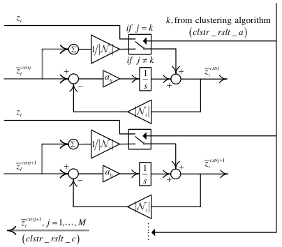
In this subsection, the distributed clustering algorithm is introduced. The feature states of the $i$-th agent are denoted by $x_{i}$ $\in\mathfrak{R}^{n}$. These feature states are used to cluster $N$ agents into $M$ clusters in real-time. The average estimations of the states $x_{i}$ in cluster $j$ are defined as $\bar{x}_{i}^{cstrj}$, in which $i=1,...,N$ and $j=1,...,M$. In all clusters, the latest average states $\bar{x}_{i}^{cstrj}$ are dynamically accessed by each $i$-th agent via the distributed communication network.

Next, the algorithm is described. The initial average estimations of $\bar{x}_{i}^{cstrj}$ are selected arbitrarily. Then, the current state $x_{i}$ is compared to all current estimations of the $\bar{x}_{i}^{cstrj}$, where $j=1,...,M$ to decide to which cluster the $i$-th agent belongs to. The $i$-th agent belongs to the $k$-th cluster if its estimated state, $\bar{x}_{i}^{cstrk}$, has the smallest distance from its current state $x_{i}$, as determined by (10). After all clusters are obtained, for each $i$-th agent, average state estimation of the $k$-th cluster is compared with its current state $x_{i}$ to decide to which cluster it belongs to and the estimations of the $k$-th cluster agents are sent to the communication network, as defined by (8). On the other hand, the state estimates of the neighbours, which are not members of the $k$-th cluster, $j\in\{1,...,N\}$, $j\neq k$, are passed through, as depicted in (9) [21].

where $|\mathcal{N}_{i}|$ is the number of neighbours of the $i$-th agent.

As depicted in Fig. 2, the following two results can always be accessed by the $i$-th agent:

1. 1.

   $clstr\_rslt\_a$: information that belongs to the $k$-th cluster;

2. 2.

   $clstr\_rslt\_b$: the average estimations of the feature states $\bar{x}_{i}^{cstrj}$ in the $j$-th cluster, $j=1,...,M$.

The dynamic clustering algorithm is summarized as Algorithm 1 and Fig. 2 illustrates the implementation of the proposed algorithm.

Within the clusters, the auxiliary states $z_{i}\in\mathfrak{R}^{m}$can be used for analysis. Therefore, the estimations of the auxiliary state, $z_{i}$ are defined as $\bar{z}_{i}^{cstrj}$, where $i=1,...,N$ and $j=1,...,M$. Similar to the estimations of the average state, $\bar{x}_{i}^{cstrj}$ from Algorithm 1, the $\bar{z}_{i}^{cstrk}$ can be obtained using the result of $clstr\_rslt\_a$. Then, the same procedure as for the estimations of the feature state is followed [21],

The result of $clstr\_rslt\_c$ is accessed by the $i$-th agent node via the distribution network as illustrated in Fig. 3.

Algorithm 2 is obtained by including the average estimations of auxiliary states into Algorithm 1.

Methodology for the distributed clustering algorithm with dynamic power balancing control can be described as follows:

1. 1.

   In a given bus, the active powers among the three phases should be equally balanced, a sum of the phase currents is equal to zero ($I_{a}+I_{b}+I_{c}=0$). It is assumed that there are nine households connected to a bus, and three households to a phase, as shown in Fig. 1.

2. 2.

   Algorithm 1 is required to group the households at the same bus into three clusters (phases $a$, $b$ and $c$) by using the phase shifts in (II-B) as the feature states. Virtual communication links are formed as shown in Fig. 4. A cluster of Agents $1$-$3$ represents the households belonging to phase $a$, while the other two household clusters belong to phases $b$ and $c$.

3. 3.

   Algorithm 2 is adopted for utilization of the feature states within the cluster. In this step, the grid power exchanges ($P_{g}^{i\phi}$) are calculated using (4) and are subsequently sent to the other two clusters. (Note that each cluster has to be able to communicate with the neighbouring clusters.)

4. 4.

   Next, two possible decisions can be made by the power balancing control method. If the the grid power exchanges ($P_{g}^{i\phi}$) have the same sign (either injected power or consumed power from the grid), ESs’ powers ($P_{b}^{i\phi}$) for balancing operation are calculated using (13). However, if the grid power exchanges ($P_{g}^{i\phi}$) have opposite signs (both delivered and consumed powers), (14) along with (15) and (16) are used to calculate the ESs’ powers ($P_{b}^{i\phi}$).

5. 5.

   After ESs’ powers ($P_{b}^{i\phi}$) are obtained, charge/discharge currents of the ES devices are calculated using (5) to obtain the reference signals for the power control loop. In this step, $SoC_{max}$ and $SoC_{min}$ of the ES devices are taken into consideration to ensure that all ES devices operate within the limits.

6. 6.

   In a realistic situation, not all households may be willing to participate in the power balancing control even though they have sufficient power. In this case, the average state estimations in the clustering algorithm will not include the unwilling households in the power control operation.

7. 7.

   Furthermore, SoC condition may be taken into consideration. Batteries having a certain SoC, eg close to $50\%$, are more suitable to participate in the power balancing control. The households having too high or too low SoCs may not be allowed to participate into power control even though they are willing to.

There are three possible scenarios of the grid power exchanges in the four-wire multi-grounded LV distribution system illustrated in Fig. 5 :

Fig. 6 depicts the complete control system of the proposed control strategy for the $i$-th ES system.

1. 1.

   Green block shows the distributed clustering algorithm and the auxiliary states estimations. In the clustering algorithm block, the phase shift in (II-B) is the pre-selected feature state $x_{i}$. In this block, a virtual ES system is formed at each phase at a given bus. Within the cluster, the obtained auxiliary average states $\bar{z}_{i}^{cstrk}=$ $P_{g}^{i\phi}$ ($=P_{l}^{i\phi}-P_{pv}^{i\phi}$) are sent to the neighbours and to the power balancing control.

2. 2.

   Red block represents the dynamic power balancing control. In this block, the grid power exchanges from the other two phases are received from the neighbours. Hence, the battery current in (5) for the power balancing can be obtained.

3. 3.

   Purple block indicates that the current from the dynamic power balancing control is the reference signal for the power control block at the primary level control. The converter controller generates the PWM signal for the converter to achieve the power balancing control.

References

- [1] M. J. Hossain, F. H. M. Rafi, G. Town, and J. Lu, “Multifunctional three-phase four-leg pv-svsi with dynamic capacity distribution method,” IEEE Transactions on Industrial Informatics, vol. 14, no. 6, pp. 2507–2520, 2018.
- [2] J. Balda, A. Oliva, D. McNabb, and R. Richardson, “Measurements of neutral currents and voltages on a distribution feeder,” IEEE Transactions on Power Delivery, vol. 12, no. 4, pp. 1799–1804, 1997.
- [3] T. M. Gruzs, “A survey of neutral currents in three-phase computer power systems,” IEEE Transactions on Industry Applications, vol. 26, no. 4, pp. 719–725, 1990.
- [4] D. W. Zipse, “The hazardous multigrounded neutral distribution system and dangerous stray currents,” in IEEE Industry Applications Society 50th Annual Petroleum and Chemical Industry Conference, 2003. Record of Conference Papers. IEEE, 2003, pp. 23–45.
- [5] A. M. Lefcourt, Effects of electrical voltage/current on farm animals: How to detect and remedy problems. United States Dept. of Agriculture, Agriculture Research Service, 1991.
- [6] T. C. Surbrook, N. D. Reese, and A. M. Kehrle, “Stray voltage: Sources and solutions,” IEEE transactions on industry applications, no. 2, pp. 210–215, 1986.
- [7] J. Zhu, M.-Y. Chow, and F. Zhang, “Phase balancing using mixed-integer programming [distribution feeders],” IEEE transactions on power systems, vol. 13, no. 4, pp. 1487–1492, 1998.
- [8] Y.-Y. Hsu, J.-H. Yi, S. Liu, Y. Chen, H. Feng, and Y. Lee, “Transformer and feeder load balancing using a heuristic search approach,” IEEE transactions on power systems, vol. 8, no. 1, pp. 184–190, 1993.
- [9] M. J. E. Alam, K. M. Muttaqi, and D. Sutanto, “Community energy storage for neutral voltage rise mitigation in four-wire multigrounded lv feeders with unbalanced solar pv allocation,” IEEE Transactions on Smart Grid, vol. 6, no. 6, pp. 2845–2855, 2015.
- [10] K. D. Hoang and H.-H. Lee, “Accurate power sharing with balanced battery state of charge in distributed dc microgrid,” IEEE Transactions on Industrial Electronics, vol. 66, no. 3, pp. 1883–1893, 2018.
- [11] M. J. E. Alam, K. M. Muttaqi, and D. Sutanto, “Alleviation of neutral-to-ground potential rise under unbalanced allocation of rooftop pv using distributed energy storage,” IEEE Transactions on Sustainable Energy, vol. 6, no. 3, pp. 889–898, 2015.
- [12] J. Han, J. Pei, and M. Kamber, Data mining: concepts and techniques. Elsevier, 2011.
- [13] S.-S. Yu, S.-W. Chu, C.-M. Wang, Y.-K. Chan, and T.-C. Chang, “Two improved k-means algorithms,” Applied Soft Computing, vol. 68, pp. 747–755, 2018.
- [14] A. B. Geva, “Hierarchical unsupervised fuzzy clustering,” IEEE transactions on fuzzy systems, vol. 7, no. 6, pp. 723–733, 1999.
- [15] J. A. Flanagan, “Self-organisation in kohonen’s som,” Neural networks, vol. 9, no. 7, pp. 1185–1197, 1996.
- [16] M. Aci and M. Avci, “K nearest neighbor reinforced expectation maximization method,” Expert Systems with Applications, vol. 38, no. 10, pp. 12 585–12 591, 2011.
- [17] N. K. Visalakshi and K. Thangavel, “Distributed data clustering: a comparative analysis,” in Foundations of Computational, IntelligenceVolume 6. Springer, 2009, pp. 371–397.
- [18] M. Hai, S. Zhang, L. Zhu, and Y. Wang, “A survey of distributed clustering algorithms,” in 2012 International Conference on Industrial Control and Electronics Engineering. IEEE, 2012, pp. 1142–1145.
- [19] A. D. Kolagar, P. Hamedani, and A. Shoulaie, “The effects of transformer connection type on voltage and current unbalance propagation,” in 2012 3rd Power Electronics and Drive Systems Technology (PEDSTC). IEEE, 2012, pp. 308–314.
- [20] T. Kim and W. Qiao, “A hybrid battery model capable of capturing dynamic circuit characteristics and nonlinear capacity effects,” IEEE Transactions on Energy Conversion, vol. 26, no. 4, pp. 1172–1180, 2011.
- [21] R. Zhang and B. Hredzak, “A novel dynamic peer-to-peer clustering algorithm and its application to aggregate energy storage systems,” arXiv preprint arXiv:1901.10029, 2019.
- [22] F. L. Lewis, H. Zhang, K. Hengster-Movric, and A. Das, Cooperative control of multi-agent systems: optimal and adaptive design approaches. Springer Science & Business Media, 2013.