A high-order / low-order (HOLO) algorithm for preserving conservation in time-dependent low-rank transport calculationsJournal: Elsevier

Zhuogang Peng Email: zpeng5@nd.edu Address: Department of Aerospace and Mechanical Engineering, University of Notre Dame, Notre Dame, IN, 46545, USA Ryan McClarren Email: rmcclarren@nd.edu Corresponding author: Corresponding author Address: Department of Aerospace and Mechanical Engineering, University of Notre Dame, Notre Dame, IN, 46545, USA

Abstract

Dynamical low-rank (DLR) approximation methods have previously been developed for time-dependent radiation transport problems. One crucial drawback of DLR is that it does not conserve important quantities of the calculation, which limits the applicability of the method. Here we address this conservation issue by solving a low-order equation with closure terms computed via a high-order solution calculated with DLR. We observe that the high-order solution well approximates the closure term, and the low-order solution can be used to correct the conservation bias in the DLR evolution. We also apply the linear discontinuous Galerkin method for the spatial discretization to obtain the asymptotic limit. We then demonstrate with the numerical results that this so-called high-order / low-order (HOLO) algorithm is conservative without sacrificing computational efficiency and accuracy.

Keywords:

Dynamical low-rank approximation, Radiation transport, Discontinuous Galerkin, Spherical Harmonics

1 Introduction

The radiation transport equation (RTE) describes the movement of particles (e.g., photons or neutrons) through a background medium. Solving the RTE is of great interest across many research areas, namely, nuclear engineering [1], astrophysics [2], and optics [3]. It is a challenging problem because the RTE has seven independent variables, including one in time, three in position, two in direction, and one in energy, which requires an extravagant computational burden in terms of both memory and operations. Thus, developing a computationally inexpensive, yet accurate, algorithm is a continuing concern.

There is a long history of methods designed to reduce the complexity and size of radiation transport calculations. Many of these efforts have focused on the direction, or angular, variables. The diffusion method, and its flux-limited variants [4, 5, 6, 7], represent the direction variables with a two-moment representation based on Fick’s law. Nevertheless, a two-moment description of the directional variables is inadequate to describe the behaviour in many problems [8]. The expansion order can be increased by using spherical harmonics methods [9, 10], though these methods have limitations, including negative densities [11], that need to be addressed with either filters [12, 13, 14, 15], or nonlinear closures that increase in the computational complexity [16, 17, 18, 19, 20]. The simplified spherical harmonics method [21], is an intermediate approximation between the diffusion method and spherical harmonics [22], that also has issues with accurately solving many problems [23]. Recent work on wavelets [24, 25, 26] and adaptive discrete ordinates methods [27, 28, 29] have shown that it is possible to reduce complexity by focusing the effort on angular degrees where most necessary.

Alongside the investigations into angular discretizations, there is a record of work addressing the other complexities in transport problems. This includes the so-called second-order forms such as the even-parity, odd-parity [30], self-adjoint [31], and least-squares [32, 33] forms. The second-order forms in many cases require the solution of half the number of equations with the additional benefits that spatial discretizations of second-operators possess [34, 35]. The second-order forms do have issues in voids [36, 37, 38] that cause either inaccuracy or loss of the self-adjoint character of the equations. Adaptivity in space [39, 40, 41, 42] and space-angle [43], as well as selective reduction of degrees of freedom [44] have all been explored as well.

In this paper, we continue a more recent trend of applying dynamical low-rank (DLR) approximation methods to radiation transport problems. These methods project the RTE onto a reduced basis in space and angle that evolves dynamically during a calculation. DLR methods were considered for the RTE in work by the authors [45]. The idea of this method comes from a conventional paradigm in solving the time-dependent Schrödinger equation for multidimensional dynamical systems, known as Multi-Configuration Time-Dependent Hartree (MCTDH), which gives a rank-1 approximation for a multivariate wave function [46]. The DLR approximates the time derivative of the objective matrices or tensors by applying tangent space projection [47, 48, 49]. It was shown to be robust even with small singular values [50] when the time integration is performed using splitting [51, 52]. The application in other kinetic equations can be found in [53, 54, 55]. The implementation in radiation transport calculations produces high-fidelity results obtained from the low-rank scheme with a fraction of memory usage and computational time. However, this approach does not preserve the total number of particles (i.e., the methods are not guaranteed to be conservative), which may result in a significant error at long times or in steady-state. There is an attempt to recover the conservation by enforcing the conservation law to the low-rank scheme, which results in an optimization problem that needs to be solved [56] that increases the computational cost of the method.

In this paper, we propose a high-order/low-order (HOLO) algorithm [57, 58] to solve this conservation issue. In our algorithm, we take the high-order, low-rank solution to calculate a closure term in the low-order two-moment approximation of the transport equation, in an approach very similar to the quasi-diffusion method [59, 60]. The low-order system conserves particles independent of the closure. This allows us to demonstrate that our HOLO algorithm overcomes the conservation difficulty while preserving the computational efficiency and accuracy. Additionally, we demonstrate that this approach can also preserve the asymptotic diffusion limit [61, 62] of the radiation transport equation.

We begin with a brief review of the low-rank method in Section 2. Then we present the low-order system with the closure term to preserve the number of particles. We further introduce the HOLO scheme which couples the low-order system with the low-rank solutions. To guarantee the consistency between the two systems, we develop a moment-based correction method to fix the conservation in the low-rank evolution. After that, we design a numerical scheme for the 2-D RTE with a discontinuous Galerkin discretization in space and a spherical harmonic (P_N) expansion in angle. In our results section, we demonstrate the efficacy of our algorithm with numerical results to validate the memory-reduction, conservation and asymptotic preserving properties.

2 Dynamical low-rank approximation

We consider a time-dependent radiative transfer equation with one energy group:

\begin{split}\frac{1}{c}\frac{\partial\psi(\bm{r},\hat{\Omega},t)}{\partial t}+\hat{\Omega}\bm{\cdot}\bm{\nabla}\psi(\bm{r},\hat{\Omega},t)+\sigma_{\mathrm{t}}(\bm{r})\psi(\bm{r},\hat{\Omega},t)=\frac{1}{4\pi}\sigma_{\mathrm{s}}(\bm{r})\phi(\bm{r},t)+Q(\bm{r},t).\end{split}

(1)

The radiation intensity $\psi(\bm{r},\hat{\Omega},t)$ [energy/area/steradian/time] is a function of position $\bm{r}$ , time $t$ , and the unit angle vector $\hat{\Omega}(\mu,\varphi)$ , where $\mu$ is the cosine of the polar angle and $\varphi$ is the azimuthal angle. The total and isotropic scattering macroscopic cross-sections with units of inverse length are denoted as $\sigma_{t}(\bm{r})$ and $\sigma_{s}(\bm{r})$ , respectively, $c$ is the particle speed, and $Q(\bm{r},t)$ is a prescribed source. We set c = 1 in the following derivations for simplicity. The scalar intensity, $\phi(\bm{r},t)$ , is the integral of $\psi(\bm{r},\hat{\Omega},t)$ over all angles:

\phi(\bm{r},t)=\int_{4\pi}\psi(\bm{r},\hat{\Omega},t)\,d\hat{\Omega}.

(2)

The low-rank method aims to approximate the solution to Eq. (1) with rank $r$ using the form

\psi(\bm{r},\hat{\Omega},t)\approx\sum_{i,j=1}^{r}X_{i}(\bm{r},t)S_{ij}(t)W_{j}(\hat{\Omega},t);

(3)

where $X_{i}$ is an orthonormal basis for $\bm{r}$ and $W_{j}$ is an orthonormal basis for $\hat{\Omega}$ using the inner products

\langle f,g\rangle_{\bm{r}}=\int_{D}fg\,d\bm{r},\quad\langle f,g\rangle_{\hat{\Omega}}=\int_{4\pi}fg\,d\hat{\Omega}.

The expansion is unique with orthonormality $\langle X_{i},{X}_{j}\rangle_{\bm{r}}=\langle W_{i},{W}_{j}\rangle_{\hat{\Omega}}=\delta_{ij}$ and gauge conditions $\langle X_{i},\dot{X}_{j}\rangle_{\bm{r}}=0$ and $\langle W_{i},\dot{W}_{j}\rangle_{\hat{\Omega}}=0$ . The rank $r$ should be less than the number the degrees of freedom in the either of the bases $X_{i}$ and $W_{j}$ . We then define the orthogonal projectors to the low-rank ansatz spaces $\bar{X}=\{X_{1},X_{2},...,X_{r}\}$ and $\bar{W}=\{W_{1},W_{2},...,W_{r}\}$ as

P_{\bar{X}}g=\sum_{i=1}^{r}X_{i}\langle X_{i}g\rangle_{\bm{r}},

(4)

P_{\bar{W}}g=\sum_{j=1}^{r}W_{j}\langle W_{j}g\rangle_{\hat{\Omega}}.

(5)

The full solution $\psi(\bm{r},\hat{\Omega},t)$ can be projected into the low-rank manifold $\mathcal{M}_{r}$ by the projector $Pg=P_{\bar{W}}g-P_{\bar{X}}P_{\bar{W}}g+P_{\bar{X}}g$ . To make the computation more robust, we split the process into three steps [51], where we solve each of the following three equations over a time step:

\partial_{t}\psi(\bm{r},\hat{\Omega},t)=P_{\bar{W}}\bigg(-\hat{\Omega}\cdot\bm{\nabla}\psi(\bm{r},\hat{\Omega},t)-\sigma_{t}(\bm{r},t)\psi(\bm{r},\hat{\Omega},t)\\ +\frac{1}{4\pi}\sigma_{\mathrm{s}}(\bm{r},t)\phi(\bm{r},t)+Q(\bm{r},t)\bigg),

(6)

\partial_{t}\psi(\bm{r},\hat{\Omega},t)=-P_{\bar{X}}P_{\bar{W}}\bigg(-\hat{\Omega}\cdot\bm{\nabla}\psi(\bm{r},\hat{\Omega},t)-\sigma_{t}(\bm{r},t)\psi(\bm{r},\hat{\Omega},t)\\ +\frac{1}{4\pi}\sigma_{\mathrm{s}}(\bm{r},t)\phi(\bm{r},t)+Q(\bm{r},t)\bigg),

(7)

\partial_{t}\psi(\bm{r},\hat{\Omega},t)=P_{\bar{X}}\bigg(-\hat{\Omega}\cdot\bm{\nabla}\psi(\bm{r},\hat{\Omega},t)-\sigma_{t}(\bm{r},t)\psi(\bm{r},\hat{\Omega},t)\\ +\frac{1}{4\pi}\sigma_{\mathrm{s}}(\bm{r},t)\phi(\bm{r},t)+Q(\bm{r},t)\bigg).

(8)

We then formulate the projections (6) - (8) explicitly from time $t_{0}$ to $t_{0}+h$ where $h$ is the step size. To simplify the notation we define $K_{j}(\bm{r},t)=\sum^{r}_{i}X_{i}(\bm{r},t)S_{ij}(t)$ and $L_{i}=\sum_{j}^{r}S_{ij}(t)W_{j}(\hat{\Omega},t)$ . The corresponding projected equations are

\partial_{t}K_{j}=-\sum_{l=1}^{r}\bm{\nabla}K_{l}\,\langle\hat{\Omega}W_{l}W_{j}\rangle_{\hat{\Omega}}-\sigma_{\mathrm{t}}K_{j}+\frac{1}{4\pi}\sigma_{\mathrm{s}}\sum_{l=1}^{r}K_{l}\langle W_{l}\rangle_{\hat{\Omega}}\langle W_{j}\rangle_{\hat{\Omega}}\\ +Q\langle W_{j}\rangle_{\hat{\Omega}},

(9)

\frac{d}{dt}S_{ij}=\sum_{kl}^{r}\langle\bm{\nabla}X_{k}\,X_{i}\rangle_{\bm{r}}S_{kl}\langle\hat{\Omega}W_{l}W_{j}\rangle_{\hat{\Omega}}+\sum_{k}^{r}\langle\sigma_{t}X_{k}X_{i}\rangle_{\bm{r}}S_{kj}\\ -\frac{1}{4\pi}\sum_{kl}^{r}\langle\sigma_{s}X_{k}X_{i}\rangle_{\bm{r}}S_{kl}\langle W_{l}\rangle_{\hat{\Omega}}\langle W_{j}\rangle_{\hat{\Omega}}-\langle X_{i}Q\rangle_{\bm{r}}\langle W_{j}\rangle_{\hat{\Omega}},

(10)

\frac{d}{dt}L_{i}=-\hat{\Omega}\sum_{k}^{r}\langle\bm{\nabla}X_{k}\,X_{i}\rangle_{\bm{r}}L_{k}-\sum_{k}^{r}\langle\sigma_{t}X_{k}X_{i}\rangle_{\bm{r}}L_{k}\\ +\frac{1}{4\pi}\sum_{k}^{r}\langle\sigma_{s}X_{k}X_{i}\rangle_{\bm{r}}\langle L_{k}\rangle_{\hat{\Omega}}+\langle QX_{i}\rangle_{\bm{r}}.

(11)

We summarize the procedures to solve equations (9) - (11) in Algorithm 1. Importantly, in the algorithm only the low-rank components $X$ , $S$ and $W$ are stored during the time evolution rather than the full solution $\psi$ . This allows the low-rank method to save computer memory.

Given
-initial time

t_{0}

-time step

h

-desired rank

r

-initial condition

\psi^{(0)}(\bm{r},\hat{\Omega},t_{0})

-initial approximations

X^{(0)}_{i}(\bm{r},t_{0})

S^{(0)}_{ij}(t_{0}),W^{(0)}_{j}(\hat{\Omega},t_{0})

Repeat:
-

t_{1}=t_{0}+h

-Solve equation (9) for

K_{j}^{(1)}(\bm{r},t_{1})

with initial condition

K_{j}^{(0)}(\bm{r},t_{0})=\sum^{r}_{i}X_{i}^{(0)}S_{ij}^{(0)}

and then factor into

X_{i}^{(1)}(\bm{r},t_{1})

and

S_{ij}^{(1)}(t_{1})

using a QR decomposition;

W_{j}^{(1)}=W_{j}^{(0)}

is preserved in this step.
-Solve equation (10) for

S_{ij}^{(2)}(t_{1})

with initial condition

S_{ij}^{(2)}(t_{0})=S_{ij}^{(1)}

X_{i}^{(2)}=X_{i}^{(1)}

and

W_{j}^{(2)}=W_{j}^{(1)}

are preserved in this step.
-Solve equation (11) for

L_{i}^{(3)}(\hat{\Omega},t_{1})

with initial condition

L_{i}^{(3)}(\hat{\Omega},t_{0})=\sum^{r}_{j}S_{ij}^{(2)}W_{j}^{(2)}

and then factor into

S_{ij}^{(3)}(t_{1})

and

W_{j}^{(3)}(\hat{\Omega},t_{1})

using a QR decomposition;

X_{i}^{(3)}=X_{i}^{(2)}

is preserved in this step.
-

t_{0}=t_{1}

X_{i}^{(0)}=X_{i}^{(3)}

S_{ij}^{(0)}=S_{ij}^{(3)}

W_{j}^{(0)}=W_{j}^{(3)}

Algorithm 1 Dynamical low-rank approximation

3 HOLO algorithm

In this section we will construct the low-order system that requires closure terms. We apply the quasi-diffusion method [59] which is also known as the variable Eddington factor method [63], to Eq. (1) to yield a two-angular-moments formulation [8]:

\frac{1}{c}\frac{\partial\phi(\bm{r},t)}{\partial t}+\bm{\nabla}\bm{\cdot}J(\bm{r},t)+\sigma_{\mathrm{t}}(\bm{r})\phi(\bm{r},t)=\sigma_{\mathrm{s}}(\bm{r})\phi(\bm{r},t)+Q(\bm{r},t).

(12)

and

\frac{1}{c}\frac{\partial J(\bm{r},t)}{\partial t}+\bm{\nabla}\bm{\cdot}\chi\phi(\bm{r},t)+\sigma_{\mathrm{t}}(\bm{r})J(\bm{r},t)=0.

(13)

where

J(\bm{r},t)=\int_{4\pi}\hat{\Omega}\psi(\bm{r},\hat{\Omega},t)\,d\hat{\Omega}

(14)

is the radiative flux (or current density), and

\chi=\frac{\int_{4\pi}\hat{\Omega}\otimes\hat{\Omega}\psi(\bm{r},\hat{\Omega},t)\,d\hat{\Omega}}{\phi(\bm{r},t)}

(15)

is the Eddington tensor and $\otimes$ denotes the outer product. Note that $\phi$ is the zeroth moment, $J$ is the first moment and $\chi$ is the normalized second moment related to radiation pressure. To close Eqs. (12) and (13) we need to evaluate the Eddington tensor $\chi$ . An approximation $\chi\approx\frac{1}{3}I$ , used in the diffusion method, is based on the assumption that $\psi$ is a linear function of angle, where $I$ is an identity tensor. Such approximations ignore the relation of Eddington factor to higher order moments, which limits their accuracy.

We propose a closure term $\gamma=\bm{\nabla}\bm{\cdot}\frac{1}{3}\phi(\bm{r},t)-\bm{\nabla}\bm{\cdot}\chi\phi(\bm{r},t)$ added to the right hand side of Eq. (13) that corrects the $\chi\approx\frac{1}{3}I$ approximation based on the solution to the full RTE. The corrected equation that we solve is

\frac{1}{c}\frac{\partial J(\bm{r},t)}{\partial t}+\frac{1}{3}\bm{\nabla}\bm{\cdot}\phi(\bm{r},t)+\sigma_{\mathrm{t}}(\bm{r})J(\bm{r},t)=\gamma(\bm{r},t).

(16)

As we will show later, $\gamma$ is calculated as the difference between the low-rank equations (9) - (11) and the quasi-diffusion equation (12) - (13). The main idea of our HOLO algorithm is that the solution to the low-order system (12) and (16) can be accurate if $\gamma$ is evaluated through the solution to the high-order system (9 - 11). Additionally, the solution is conservative in $\phi$ regardless of the value of the closure term because $J$ appears in conservative form in Eq. (12).

3.1 Angular discretization for low-rank equations in 2D

We choose the angular bases $W_{j}(\mu,\varphi,t)$ to be the spherical harmonics expansion truncated at $N$ :

W_{j}(\mu,\varphi,t)\approx\sum_{l=0}^{N}\,\sum_{k=0}^{l}v_{jlk}(t)Y_{l}^{k}(\mu,\varphi)

(17)

where

Y_{l}^{k}(\mu,\varphi)=\sqrt{\frac{2l+1}{4\pi}\,\frac{(l-k)!}{(l+k)!}}\,P_{l}^{k}(\mu)\,e^{i\,k\varphi},

where $P_{l}^{k}(\mu)$ is the associate Legendre polynomial and $N$ is the expansion order. Here $0\leq k\leq l\leq N$ and the negative $k$ are omitted because of the symmetry properties of the spherical harmonics [64]. The total number of moments is $n=\frac{(N+1)(N+2)}{2}$ .

We use vectors ${V_{j}}$ to collect all the angular elements $v_{jlk}$ in $W_{j}$ and $\bm{Y}$ for all the spherical harmonics $Y_{l}^{k}$ sorted by the index $l$ , e.g., $\bm{Y}=[Y_{0}^{0},\ Y_{1}^{0},\ Y_{1}^{1},\ Y_{2}^{0},\ ...\ Y_{N}^{N}]^{T}$ . The integration of $\bm{Y}$ in angular domain is computed as

\int_{0}^{2\pi}\int_{-1}^{1}\bm{Y}\,d\mu d\varphi=\langle\bm{Y}\rangle=[2\sqrt{\pi},0,0,...0]

for later use. We then substitute the angular basis $W_{j}=Y^{T}V_{j}$ into the projection Eqs. (9) and (10):

\partial_{t}K_{j}=-\sum_{l=1}^{r}\partial_{z}K_{l}{V_{l}}^{T}\bm{A_{z}}{V_{j}}-\sum_{l=1}^{r}\partial_{x}K_{l}{V_{l}}^{T}\bm{A_{x}}{V_{j}}-\sigma_{\mathrm{t}}K_{j}\\ +\frac{1}{4\pi}\sigma_{\mathrm{s}}\sum_{l=1}^{r}K_{l}{V_{l}}^{T}\langle\bm{Y}\rangle\langle\bm{Y}\rangle^{T}\,{V_{j}}+Q\int_{0}^{2\pi}\int_{-1}^{1}\langle\bm{Y}\rangle^{T}\,V_{j},

(18)

\frac{d}{dt}S_{ij}=\sum_{kl}^{r}\langle\partial_{z}X_{k}\,X_{i}\rangle_{\bm{r}}S_{kl}{V_{l}}^{T}\bm{A_{z}}{V_{j}}+\sum_{kl}^{r}\langle\partial_{x}X_{k}\,X_{i}\rangle_{\bm{r}}S_{kl}{V_{l}}^{T}\bm{A_{x}}{V_{j}}\\ +\sum_{k}^{r}\langle\sigma_{t}X_{k}X_{i}\rangle_{\bm{r}}S_{kj}-\frac{1}{4\pi}\sum_{kl}^{r}\langle\sigma_{s}X_{k}X_{i}\rangle_{\bm{r}}S_{kl}{V_{l}}^{T}\langle\bm{Y}\rangle\langle\bm{Y}\rangle^{T}{V_{j}}\\ -\langle X_{i}Q\rangle_{\bm{r}}\langle\bm{Y}\rangle^{T}\,V_{j},

(19)

Note that $A_{x}=\int_{0}^{2\pi}\int_{-1}^{1}\sqrt{1-\mu^{2}}\cos\varphi\bm{Y}\bm{Y}^{T}\ d\mu d\varphi$ , and $A_{z}=\int_{0}^{2\pi}\int_{-1}^{1}\mu\bm{Y}\bm{Y}^{T}\ d\mu d\varphi$ can be calculated using the recursion property and no quadrature rule is required.

We multiply $\bm{Y}$ on both sides of Eq. (11) and integrate over all angles to remove the angular dependence:

\frac{d}{dt}R_{i}=-\sum_{k}^{r}\langle\partial_{z}X_{k}\,X_{i}\rangle_{\bm{r}}R_{k}\bm{A_{z}}-\sum_{k}^{r}\langle\partial_{x}X_{k}\,X_{i}\rangle_{\bm{r}}R_{k}\bm{A_{x}}+\sum_{k}^{r}\langle\sigma_{t}X_{k}X_{i}\rangle_{\bm{r}}R_{k}\\ -\frac{1}{4\pi}\sum_{k}^{r}\langle\sigma_{s}X_{k}X_{i}\rangle_{\bm{r}}R_{k}\langle\bm{Y}\rangle\langle\bm{Y}\rangle^{T}-\langle X_{i}Q\rangle_{\bm{r}}\langle\bm{Y}\rangle^{T}

(20)

where $R_{i}=\int_{0}^{2\pi}\int_{-1}^{1}L_{i}(t,\mu,\varphi)\bm{Y}^{T}\,d\mu d\varphi$ . The low-rank P_N moments can be obtained from

\psi_{l}^{k}(x,z,t)=\int_{0}^{2\pi}\int_{-1}^{1}\psi(x,z,\mu,\varphi,t)Y_{l}^{k}(\mu,\varphi)\,d\mu d\varphi=\sum_{ij}^{r}X_{i}(x,z,t)S_{ij}(t)v_{jlk}(t).

3.2 Time evolution and consistency

The quantities in our low-order system are related to the spherical harmonics moments by

\begin{split}&\phi(x,z,t)=2\sqrt{\pi}\psi_{0}^{0}(x,z,t),\\ &J(x,z,t)=\begin{bmatrix}J_{z}(x,z,t)\\ J_{x}(x,z,t)\end{bmatrix}=\begin{bmatrix}2\sqrt{\frac{\pi}{3}}\psi_{1}^{0}(x,z,t)\\ -2\sqrt{\frac{2\pi}{3}}\psi_{1}^{1}(x,z,t)\end{bmatrix},\\ &\gamma(x,z,t)=\begin{bmatrix}2\sqrt{\frac{\pi}{3}}\gamma_{z}(x,z,t)\\ -2\sqrt{\frac{2\pi}{3}}\gamma_{x}(x,z,t)\end{bmatrix}.\end{split}

(21)

We substitute (21) into the quasi-diffusion approximation (12) and (16) to get an equivalent P₁ system

\begin{split}&\frac{\partial\phi_{0}^{0}}{\partial t}+\sqrt{\frac{1}{3}}\frac{\partial\phi_{1}^{0}}{\partial z}-\sqrt{\frac{2}{3}}\frac{\partial\phi_{1}^{1}}{\partial x}=\left(\sigma_{\mathrm{s}}-\sigma_{\mathrm{t}}\right)\phi_{0}^{0}+\frac{1}{2\sqrt{\pi}}Q.\\ &\frac{\partial\phi_{1}^{0}}{\partial t}+\sqrt{\frac{1}{3}}\frac{\partial\phi_{0}^{0}}{\partial z}=-\sigma_{\mathrm{t}}\phi_{0}^{0}+\gamma_{z}\\ &\frac{\partial\phi_{1}^{1}}{\partial t}-\sqrt{\frac{1}{6}}\frac{\partial\phi_{0}^{0}}{\partial x}=-\sigma_{\mathrm{t}}\phi_{0}^{0}+\gamma_{x}\\ \end{split}.

(22)

In this work, we adopt the forward Euler method for the time integration. At a time step from $t_{n}$ to $t_{n+1}=t_{n}+\Delta t$ , we calculate the closure terms in (22) through equations

\begin{split}&\gamma_{z}\big|_{n}=\frac{\phi_{1}^{0}\big|^{HO}_{n+1}-\phi_{1}^{0}\big|^{HO}_{n}}{\Delta t}+\sqrt{\frac{1}{3}}\frac{\partial\phi_{0}^{0}\big|^{HO}_{n}}{\partial z}+\sigma_{\mathrm{t}}\phi_{0}^{0}\big|^{HO}_{n},\\ &\gamma_{x}\big|_{n}=\frac{\phi_{1}^{1}\big|^{HO}_{n+1}-\phi_{1}^{1}\big|^{HO}_{n}}{\Delta t}-\sqrt{\frac{1}{6}}\frac{\partial\phi_{0}^{0}\big|^{HO}_{n}}{\partial x}+\sigma_{\mathrm{t}}\phi_{0}^{0}\big|^{HO}_{n}.\end{split}

(23)

where the three angular moments are solved from the high-order system (18 - 20). Then we use the definitions for $\gamma_{x}\big|_{n}$ and $\gamma_{z}\big|_{n}$ and solve the following low-order system

\begin{split}&\frac{\phi_{0}^{0}\big|^{LO}_{n+1}-\phi_{0}^{0}\big|^{LO}_{n}}{\Delta t}+\sqrt{\frac{1}{3}}\frac{\partial\phi_{1}^{0}\big|^{LO}_{n}}{\partial z}-\sqrt{\frac{2}{3}}\frac{\partial\phi_{1}^{1}\big|^{LO}_{n}}{\partial x}=\left(\sigma_{\mathrm{s}}-\sigma_{\mathrm{t}}\right)\phi_{0}^{0}\big|^{LO}_{n}+\frac{1}{2\sqrt{\pi}}Q\big|^{LO}_{n},\\ &\frac{\phi_{1}^{0}\big|^{LO}_{n+1}-\phi_{1}^{0}\big|^{LO}_{n}}{\Delta t}+\sqrt{\frac{1}{3}}\frac{\partial\phi_{0}^{0}\big|^{LO}_{n}}{\partial z}=-\sigma_{\mathrm{t}}\phi_{0}^{0}\big|^{LO}_{n}+\gamma_{z}\big|_{n},\\ &\frac{\phi_{1}^{1}\big|^{LO}_{n+1}-\phi_{1}^{1}\big|^{LO}_{n}}{\Delta t}-\sqrt{\frac{1}{6}}\frac{\partial\phi_{0}^{0}\big|^{LO}_{n}}{\partial x}=-\sigma_{\mathrm{t}}\phi_{0}^{0}\big|^{LO}_{n}+\gamma_{x}\big|_{n}.\end{split}

(24)

This formulation is globally conservative.

3.3 Conservation fix

Because the DLR algorithm is not conservative (as has been previously discussed), the accuracy of the closure term is limited. To overcome this drawback, we use the low-order results to update the corresponding term within the low-rank solution in every time step. We update the angular bases $W_{j}$ , as written in Eq. (17) to make the high-order and low-order solution have the same first two moments ( $\phi_{0}^{0}$ , $\phi_{1}^{0}$ and $\phi_{1}^{1}$ ). This correction can be computed without forming the full solution, preserving the low-rank representation. The formulation of the correction is given by

\sum_{j=1}^{r}(K_{j}^{\mathrm{new}}-K_{j})\begin{bmatrix}v_{j00}\\ v_{j10}\\ v_{j11}\end{bmatrix}=\begin{bmatrix}\phi_{0}^{0}\big|^{LO}\\ \phi_{1}^{0}\big|^{LO}\\ \phi_{1}^{0}\big|^{LO}\end{bmatrix}-\begin{bmatrix}\phi_{0}^{0}\big|^{HO}\\ \phi_{1}^{0}\big|^{HO}\\ \phi_{1}^{1}\big|^{HO}\end{bmatrix},

(25)

where we keep $W_{j}$ unchanged and update $X_{i}$ and $S_{ij}$ with the low-order results. This is a linear matrix equation for the $K_{j}^{\mathrm{new}}$ with a solution that can be found by least-squares. We can then factorize $K_{j}^{\mathrm{new}}$ into $X_{i}^{\mathrm{new}}$ and $S_{ij}^{\mathrm{new}}$ by QR decomposition, which are initial conditions for the next time step. The full-time evolution algorithm is given in Algorithm 2.

3.4 Reduction of Memory Requirements

The feature of memory saving in the DLR method is maintained in the HOLO algorithm. We use $m$ to denote the degrees of freedom in the spatial discretization. The memory footprint required to store the solution in each time step is

\mathrm{Memory}[\mathrm{bytes}]=8\times 2\times(mr+r^{2}+nr+3m).

(26)

The factor of 8 assumes 8 bytes per floating-point number, the factor of two comes from the fact that the previous and current time step needs to be stored, and the $3m$ accounts for the storage of $\phi$ and $J$ at the $m$ spatial degrees of freedom. The memory requirement for the full-rank update requires at least

\mathrm{Memory}[\mathrm{bytes}]=8\times 2mn.

(27)

bytes. When $r\ll m,n$ the HOLO method can require much less memory because there no quadratic terms combining $m$ and $n$ .

Given
-initial time

t_{0}

-time step

h

-desired rank

r

-initial condition

\phi_{0}(x,z,t_{0})

\phi_{1}(x,z,t_{0})

-initial approximations

X_{i}(x,z,t_{0})

S_{ij}(t_{0}),W_{j}(\mu,\varphi,t_{0})

Repeat:
-

t_{1}=t_{0}+h

-Using low-rank approximation to calculate

\psi_{l}^{k}(x,z,t_{1})=\sum_{ij}^{r}X_{i}(x,z,t_{1})S_{ij}(t_{1})v_{jlk}(t_{1})

-Calculate the closure

\gamma

with

\psi_{l}^{k}(x,z,t_{1})

using Eq. (21)
-Solve the LO system Eq. (24) for

\phi^{LO}(x,z,t_{1})

and

J^{LO}(x,z,t_{1})

-Update the low-rank bases

X_{i}(x,z,t_{1})

and

S_{ij}(t_{1})

with the LO

\phi^{LO}(x,z,t_{1})

and

J^{LO}(x,z,t_{1})

using Eq. (25)
-

t_{0}=t_{1}

Algorithm 2 HOLO algorithm

4 Spatial discretization

4.1 Low-order system

The linear conservation form of Eq. (24) is

\frac{\partial\bm{u}}{\partial_{t}}+\bm{A_{z}}^{LO}\frac{\partial\bm{u}}{\partial z}+\bm{A_{x}}^{LO}\frac{\partial\bm{u}}{\partial x}=C\bm{u}+S

(28)

where

\bm{u}=\begin{bmatrix}\phi\\ J_{z}\\ J_{x}\end{bmatrix},\,\,\,\bm{A_{x}}^{LO}=\begin{bmatrix}0&0&-\sqrt{\frac{2}{3}}\\ 0&0&0\\ -\sqrt{\frac{1}{3}}&0&0\end{bmatrix},\,\,\,\bm{A_{z}}^{LO}=\begin{bmatrix}0&\sqrt{\frac{1}{3}}&0\\ \sqrt{\frac{1}{3}}&0&0\\ 0&0&0\end{bmatrix},

C=\begin{bmatrix}\sigma_{\mathrm{s}}-\sigma_{\mathrm{t}}&0&0\\ 0&-\sigma_{\mathrm{t}}&0\\ 0&0&-\sigma_{\mathrm{t}}\end{bmatrix},\,\,\,S=\begin{bmatrix}\frac{1}{2\sqrt{\pi}}Q\\ \gamma_{z}\\ \gamma_{x}\end{bmatrix}.

We apply the bilinear discontinuous (BLD) Galerkin finite element method to discretize Eq. (28) on rectangular cells in $XZ$ geometry. The solution vector $\bm{u}$ on cell $k$ is expanded with basis functions $B_{k,i}(x,z)$

\bm{u_{k}}(x,z,t)=\sum_{i}^{4}B_{k,i}(x,z)\bm{u}_{k,i}(t),

(29)

where the basis functions are

\begin{split}B_{k,1}(x,z)=\frac{x_{R}-x}{\Delta x_{k}}\frac{z_{T}-z}{\Delta z_{k}},\\ B_{k,2}(x,z)=\frac{x-x_{L}}{\Delta x_{k}}\frac{z_{T}-z}{\Delta z_{k}},\\ B_{k,3}(x,z)=\frac{x-x_{L}}{\Delta x_{k}}\frac{z-z_{B}}{\Delta z_{k}},\\ B_{k,4}(x,z)=\frac{x_{R}-x}{\Delta x_{k}}\frac{z-z_{B}}{\Delta z_{k}}.\end{split}

(30)

The weak form of (28) is obtained by multiplying with the basis function and integrating over cell

\begin{split}\frac{d}{dt}\int_{z_{B}}^{z^{T}}dz\int_{x_{L}}^{x^{R}}dx\,B_{k,i}\bm{u_{k}}+\bm{A_{x}}\int_{z_{B}}^{z^{T}}dz\int_{x_{L}}^{x^{R}}dx\,B_{k,i}\frac{d}{d_{x}}\bm{u_{k}}\\ +\bm{A_{z}}\int_{z_{B}}^{z^{T}}dz\int_{x_{L}}^{x^{R}}dx\,B_{k,i}\frac{d}{d_{z}}\bm{u_{k}}=\\ C\int_{z_{B}}^{z^{T}}dz\int_{x_{L}}^{x^{R}}dx\,B_{k,i}\bm{u_{k}}+\int_{z_{B}}^{z^{T}}dz\int_{x_{L}}^{x^{R}}&dx\,B_{k,i}\bm{S_{k}}.\end{split}

(31)

By integrating by parts, the stream terms can be written as

\bm{A_{x}}\int_{z_{B}}^{z^{T}}dz\int_{x_{L}}^{x^{R}}dx\,B_{k,i}\frac{d}{d_{x}}\bm{u_{k}}=\bm{A_{x}}\left(\int_{z_{B}}^{z^{T}}dz\,B_{k,i}\bm{u_{k}}-\int_{z_{B}}^{z^{T}}dz\int_{x_{L}}^{x^{R}}dx\,\frac{d}{d_{x}}B_{k,i}\bm{u_{k}}\right),

and

\bm{A_{z}}\int_{z_{B}}^{z^{T}}dz\int_{x_{L}}^{x^{R}}dx\,B_{k,i}\frac{d}{d_{z}}\bm{u_{k}}=\bm{A_{z}}\left(\int_{x_{L}}^{x^{R}}dx\,B_{k,i}\bm{u_{k}}-\int_{z_{B}}^{z^{T}}dz\int_{x_{L}}^{x^{R}}dx\,\frac{d}{d_{z}}B_{k,i}\bm{u_{k}}\right).

Then we collect the vector $\bm{u}_{k}=[u_{k,1},u_{k,2},u_{k,3},u_{k,4}]^{T}$ , $\bm{B}_{k}=[B_{k,1},B_{k,2},B_{k,3},B_{k,4}]^{T}$ and $\bm{S}_{k}=[S_{k,1},S_{k,2},S_{k,3},S_{k,4}]^{T}$ to get a $4$ equation system for cell $k$

M\frac{d\bm{u}_{k}}{dt}+\bm{A_{x}}\left((L\bm{u}_{k})^{x,surf}-L_{x}\bm{u}_{k}\right)+\bm{A_{z}}\left((L\bm{u}_{k})^{z,surf}-L_{z}\bm{u}_{k}\right)=CM\bm{u}_{k}+M\bm{S}_{k},

where

M=\int_{z_{B}}^{z^{T}}dz\int_{x_{L}}^{x^{R}}dx\,\bm{B}_{k}\bm{B}_{k}^{T}=\frac{\Delta x_{k}\Delta z_{k}}{36}\begin{bmatrix}4&2&1&2\\ 2&4&2&1\\ 1&2&4&2\\ 2&1&2&4\end{bmatrix},

L_{x}=-\int_{z_{B}}^{z^{T}}dz\int_{x_{L}}^{x^{R}}dx\,\frac{\partial\bm{B}_{k}}{\partial_{x}}\bm{B}_{k}^{T}=-\frac{\Delta z_{k}}{12}\begin{bmatrix}-2&-2&-1&-1\\ 2&2&1&1\\ 1&1&2&2\\ -1&-1&-2&-2\end{bmatrix},

L_{z}=-\int_{z_{B}}^{z^{T}}dz\int_{x_{L}}^{x^{R}}dx\,\frac{\partial\bm{B}_{k}}{\partial_{z}}\bm{B}_{k}^{T}=-\frac{\Delta x_{k}}{12}\begin{bmatrix}-2&-1&-1&-2\\ -1&-2&-2&-1\\ 1&2&2&1\\ 2&1&1&2\end{bmatrix},

(L\bm{u}_{k})^{x,\mathrm{surf}}=\int_{z_{B}}^{z^{T}}dz\,\bm{B}_{k}(\bm{B}_{k}\bm{u})^{T}=\frac{\Delta z_{k}}{6}\begin{bmatrix}-2u_{k,1}^{x-}-2u_{k,4}^{x-}\\ 2u_{k,2}^{x+}+u_{k,3}^{x+}\\ u_{k,2}^{x+}+2u_{k,3}^{x+}\\ -u_{k,1}^{x-}-2u_{k,4}^{x-}\end{bmatrix},

and

(L\bm{u}_{k})^{z,\mathrm{surf}}=\int_{x_{L}}^{x^{R}}dx\,\bm{B}_{k}(\bm{B}_{k}\bm{u})^{T}=\frac{\Delta x_{k}}{6}\begin{bmatrix}-2u_{k,1}^{z-}-u_{k,2}^{z-}\\ -u_{k,1}^{z-}-2u_{k,2}^{z-}\\ 2u_{k,3}^{z+}+u_{k,4}^{z+}\\ u_{k,3}^{z+}+2u_{k,4}^{z+}\end{bmatrix}.

The superscripts indicate that the value is evaluated in the boundary, e.g., $u^{x-}_{k,1}$ is the value in the left edge of support node $1$ in cell ${k}$ . We apply the mass-matrix lumping, surface lumping and within-cell gradient term lumping techniques via the formulas:

M^{lump}_{ij}=\delta_{ij}\sum_{j^{\prime}=1}^{4}M_{ij^{\prime}},

(L\bm{u}_{k})^{\xi,\mathrm{surf,lump}}_{i,j}=\delta_{ij}\sum_{i=1}^{4}(L\bm{u}_{k})^{\xi,\mathrm{surf}},

and

L_{\xi}^{\mathrm{lump}}=\delta_{ij}\sum_{i=1}^{4}L_{ij}.

The fully lumped BLD equation is

\frac{d\bm{u}_{k}}{dt}+2\frac{\bm{A_{x}}}{\Delta_{x}}\begin{bmatrix}-u_{k,1}^{x-}\\ u_{k,2}^{x+}\\ u_{k,3}^{x+}\\ -u_{k,4}^{x-}\end{bmatrix}+\frac{\bm{A_{x}}}{\Delta_{x}}\begin{bmatrix}1&1&0&0\\ -1&-1&0&0\\ 0&0&-1&-1\\ 0&0&1&1\end{bmatrix}\bm{u}\\ +2\frac{\bm{A_{z}}}{\Delta_{z}}\begin{bmatrix}-u_{k,1}^{z-}\\ -u_{k,2}^{z-}\\ u_{k,3}^{z+}\\ u_{k,4}^{z+}\end{bmatrix}+\frac{\bm{A_{z}}}{\Delta_{z}}\begin{bmatrix}1&0&0&1\\ 0&1&1&0\\ 0&-1&-1&0\\ -1&0&0&-1\end{bmatrix}\bm{u}=C\bm{u}_{k}+S.

(32)

4.2 High-order system

We apply a similar BLD method to construct the spatial basis $X_{i}(x,z,t)$ , that is,

X_{i}(x,z,t)=\sum_{k}\sum_{q=1}^{4}Z_{k,q}(x,z)U_{k,q,i}(t)

where $Z_{k,q}(x,z)$ is the basis function with the support nodes $q$ in cell $k$ . Note that $X_{i}$ is orthogonal and $U_{k,q,i}U_{k^{\prime},q^{\prime},i^{\prime}}=\delta_{kk^{\prime}}\delta_{qq^{\prime}}\delta_{ii^{\prime}}$ is achieved by SVD or QR decomposition during our low-rank calculations. To impose the constraints to basis functions $Z_{k,q}$

\int_{z_{B}}^{z^{T}}dz\int_{x_{L}}^{x^{R}}dxZ_{k,q}Z_{k^{\prime},q^{\prime}}=\delta_{kk^{\prime}}\delta_{qq^{\prime}},

(33)

we can use the normalized basis functions $\frac{2}{\sqrt{\Delta x_{k}\Delta z_{k}}}B_{k,i}$ in each cell:

\begin{split}Z_{k,1}(x,z)=\frac{2}{\sqrt{\Delta x_{k}\Delta z_{k}}}\frac{x_{R}-x}{\Delta x_{k}}\frac{z_{T}-z}{\Delta z_{k}},\\ Z_{k,2}(x,z)=\frac{2}{\sqrt{\Delta x_{k}\Delta z_{k}}}\frac{x-x_{L}}{\Delta x_{k}}\frac{z_{T}-z}{\Delta z_{k}},\\ Z_{k,3}(x,z)=\frac{2}{\sqrt{\Delta x_{k}\Delta z_{k}}}\frac{x-x_{L}}{\Delta x_{k}}\frac{z-z_{B}}{\Delta z_{k}},\\ Z_{k,4}(x,z)=\frac{2}{\sqrt{\Delta x_{k}\Delta z_{k}}}\frac{x_{R}-x}{\Delta x_{k}}\frac{z-z_{B}}{\Delta z_{k}},\end{split}

(34)

because $\int_{z_{B}}^{z^{T}}dz\int_{x_{L}}^{x^{R}}dx\,{B}_{k,i}{B}_{k,j}=4\Delta x\Delta z\,\delta_{ij}$ .

Equation (18) can be written in a conservation form

\frac{\partial\bm{u}}{\partial t}+\bm{A_{z}}^{HO}\frac{\partial\bm{u}}{\partial z}+\bm{A_{x}}^{HO}\frac{\partial\bm{u}}{\partial x}=S(\bm{u})

(35)

where $\bm{u}=[K_{1},K_{2},...K_{r}]^{T}$ , $V=[V_{1},V_{2},...V_{r}]$ , $\bm{A_{x}}^{HO}=V^{T}\bm{A_{x}}V$ , $\bm{A_{z}}^{HO}=V^{T}\bm{A_{z}}V$ , $S(\bm{u})=-\sigma_{\mathrm{t}}K+\frac{1}{4\pi}V^{T}\langle Y\rangle\langle Y\rangle^{T}V\sigma_{\mathrm{s}}K+\frac{1}{2\sqrt{\pi}}Q$ .

There is no need to develop the weak form for Eqs. (19) and (20) but we still need to calculate spatial integration terms like $\langle\partial_{\xi}X_{p}X_{q}\rangle_{\bm{r}}$ where $\xi=x$ or $z$ :

\begin{split}\langle\partial_{\xi}X_{p}X_{q}\rangle_{\bm{r}}&=\int_{z_{B}}^{z^{T}}dz\int_{x_{L}}^{x^{R}}dx\,\partial_{\xi}\left(\sum_{k}\sum_{i}^{4}Z_{k,i}u_{k,i,p}\right)\sum_{k^{\prime}}\sum_{i^{\prime}}^{4}Z_{k^{\prime},i^{\prime}}u_{k^{\prime},i^{\prime},q}\\ &=\sum_{k,k^{\prime}}\sum_{i,i^{\prime}}u_{k,i,p}u_{k^{\prime},i^{\prime},q}\int_{z_{B}}^{z^{T}}dz\int_{x_{L}}^{x^{R}}dx\,\partial_{\xi}Z_{k,i}Z_{k^{\prime},i^{\prime}}\\ &=L_{\xi}\begin{bmatrix}\sum_{k,k^{\prime}}u_{k,p,1}u_{k,q,1}\\ \sum_{k,k^{\prime}}u_{k,p,2}u_{k,q,2}\\ \sum_{k,k^{\prime}}u_{k,p,3}u_{k,q,3}\\ \sum_{k,k^{\prime}}u_{k,p,4}u_{k,q,4}\end{bmatrix},\end{split}

(36)

where $L_{\xi}$ is the lumped matrix from Eq. (32).

4.3 Slope limiter

Here we briefly describe the slope limiter in our scheme to address artificial oscillations. First, we define $s_{k}^{x}$ as the slope in $x$ direction and $s_{k}^{z}$ in $z$ direction within each cell. Then we calculate the cell average

\bar{u}_{k}=\frac{1}{4}(u_{k,1},u_{k,2},u_{k,3},u_{k,4})

The neighbors of the cell $k$ in the left, right, top and bottom are defined as $\bar{u}_{k}^{R}$ , $\bar{u}_{k}^{L}$ , $\bar{u}_{k}^{T}$ , $\bar{u}_{k}^{B}$ , respectively. The double minmod limiter which preserves the diffusion limit [65, 66] is

s_{k}^{x}=\rm{minmod}\left(\frac{1}{2}(u_{k,2}+u_{k,3}-u_{k,1}-u_{k,4}),\rm{minmod}(\bar{u}_{k}^{R}-\bar{u}_{k},\bar{u}_{k}-\bar{u}_{k}^{L})\right)

(37)

s_{k}^{z}=\rm{minmod}\left(\frac{1}{2}(u_{k,3}+u_{k,4}-u_{k,1}-u_{k,2}),\rm{minmod}(\bar{u}_{k}^{T}-\bar{u}_{k},\bar{u}_{k}-\bar{u}_{k}^{B})\right)

(38)

where the minmod operation is given by

\rm{minmod}(a,b)=\begin{cases}\begin{aligned} a\,\,\,\,\,&\,|a|<|b|\,\,\&\,\,ab>0,\\ b\,\,\,\,\,&\,|a|>|b|\,\,\&\,\,ab>0,\\ 0\,\,\,\,\,&\,ab<0\end{aligned}\end{cases}.

(39)

From the limiter, we change the value of the four support nodes to be

\begin{split}\tilde{u}_{k,1}=\bar{u}_{k}-\frac{1}{2}s_{k}^{x}-\frac{1}{2}s_{k}^{z},\\ \tilde{u}_{k,2}=\bar{u}_{k}+\frac{1}{2}s_{k}^{x}-\frac{1}{2}s_{k}^{z},\\ \tilde{u}_{k,3}=\bar{u}_{k}+\frac{1}{2}s_{k}^{x}+\frac{1}{2}s_{k}^{z},\\ \tilde{u}_{k,4}=\bar{u}_{k}-\frac{1}{2}s_{k}^{x}+\frac{1}{2}s_{k}^{z}.\end{split}

(40)

5 Numerical Results

We demonstrate the accuracy and the computational efficiency of our HOLO algorithm with six benchmark problems. The plane source problem emphasizes the conservation fix and the modified Reed’s problem highlights the diffusion limit in a heterogeneous problem [67]. Another four 2D problems show the memory-saving feature and the benefits of high angular resolution. In all simulations the unit of length is $\mathrm{cm}$ and the particle speed is set to be $1\ \mathrm{cm/s}$ . We implement the double minmod limiter in the modified Reed’s problem and the line source problem and the minmod limiter for other problems.

5.1 Plane source problem

The plane source problem [68, 69, 70] has been used to test a variety of radiation transport methods. It describes an initial pulse of particles emitted in an infinite medium with no source and absorption, which means the total number of particles is fixed during the evolution. The main purpose of this test is to show that our HOLO algorithm is conservative without loss of computational efficiency. In the problem the initial condition is given by a Dirac-delta function placed in the center of a purely scattering media, where $\phi(x,0)=\delta(x)$ , $\sigma_{\mathrm{t}}=\sigma_{\mathrm{s}}=1$ . In all simulations, we fix the spatial resolution to $\Delta x=0.02$ , and the Courant–Friedrichs–Lewy (CFL) condition $\textrm{CFL}=\frac{c\Delta t}{\Delta x}$ to $0.2$ , where $\Delta t$ is the time step and the particle speed $c$ is set to 1. We compare the numerical solutions with the analytical benchmark given by Ganapol. Note that in 1D problems a full rank solution has $r_{\mathrm{F}}=N+1$ where $N$ is the order of the spherical harmonics.

The first set of simulations is designed to reveal what order of P_N is sufficient by comparing with results calculated by the classical full rank method. The plane source problem is considered as a difficult test because of the unavoidable oscillations. As shown in Figure 1, the magnitude of spikes in the $P_{9}$ solution is much higher than $P_{29}$ . These spikes contain uncollided particles moving at the characteristic speeds of the P_N equations. This figure also demonstrates the requirement of the high P_N order in this case because even P₂₉ has extant oscillations at the early time. From Figure 1, we can see that the order requirement is lower at a later time, and even $P_{9}$ is sufficient to capture the analytical solution. That is because there are few uncollided particles remaining at this late time.

Figure 2 presents the $P_{29}$ solutions with the low-rank method. Here the $P_{29}$ solution with rank 20, which is two-thirds of the full rank, is comparable in accuracy, as shown in Figure 2 and Figure 2. We point out that this indicates a memory reduction of roughly one-third of full rank memory. However, the conservation loss of the low-rank method is exhibited in Figure 2. Even though the solution with rank 10 approximates the shape of the true solution well, the area below the solution curve is lower than either the analytical or the numerical solutions with higher ranks due to the loss of conservation.

This issue is solved with the HOLO algorithm. As we can see from Figure 3, the $P_{29}$ solution with rank 16 is no longer lower than the analytical solution, and it is also a good approximation compared to the full rank $P_{29}$ solution. Figure 3 shows that a solution with rank 20 matches the analytical solution well. In this case the memory usage calculated by (26) is $0.185$ MB while the full rank memory is $0.230$ MB by (27), corresponding to a 20% memory savings. Though this is a modest reduction in memory, as we will see, as the number of spatial dimensions increases, the memory reduction will increase.

Refer to caption — (a) $t=1$ , $N_{x}=120$

5.2 Modified Reed’s problem

The second test is a multi-material problem that aims to verify that our numerical scheme preserves the diffusion limit. The material layout is detailed in Figure 4. Note that there are highly scattering regions, where the mean-free-path in these regions is 0.1 ( $\sigma_{\mathrm{t}}=10$ , $\sigma_{\mathrm{s}}=9.9$ ). A high-resolution and high-order full rank solution with $\Delta x=0.01$ , $P_{99}$ , CFL $=0.05$ is used as a benchmark. We then compare our HOLO solutions with different spatial resolutions and rank to the benchmark at $t=100$ , which is very near steady-state. One important finding from Figure 5 is that the solutions are not sensitive to the grid size. In strong scattering regions, all solutions match the benchmark well even with the gird size larger than the mean-free-path. We also notice that the full rank and low-rank solution with the same spatial resolution are identical on the scale of the figure.

5.3 Line source problem

The line source problem is a two-dimensional pulsed source problem. Similar to its 1D version, the initial condition is given by $\psi(x,z,0)=\delta(x)\delta(z)$ , and the total and scattering cross-section are set to 1. We compute the HOLO solution to $t=1$ in the computational domain $2.4\times 2.4$ with spatial resolution $\Delta x=\Delta z=0.02$ and CFL condition $0.2$ . Note that the total number of spatial degrees of freedom is fixed to be $m=4\ N_{x}N_{z}=57600$ , which is far larger than the number of angular bases. Thus the total memory usage is nearly independent of the order of the P_N expansion and is a stronger function of the rank, e.g, Memory (bytes) $=8\times 2\times(mr+nr+r^{2}+3m)\approx 16(r+3)m$ .

We compare the solutions with rank 300 (corresponding to the full rank $P_{23}$ ) and varying P_N orders in the following simulations. We expect the solution can be refined by keeping the rank fixed and increasing the P_N order. That is, we could have better results with a small amount of extra memory cost. Figure 6 shows the remarkable ring structure in the full rank $P_{23}$ solution. As we increase the P_N order with the HOLO algorithm, the first noticeable change is that the solution range begins to match that of the analytical solution. Furthermore, the ring structure is no longer significant in Figures 6, 6, and 6. Figure 6 presents a more straightforward comparison, where the oscillations are reduced by using more angular basis functions.

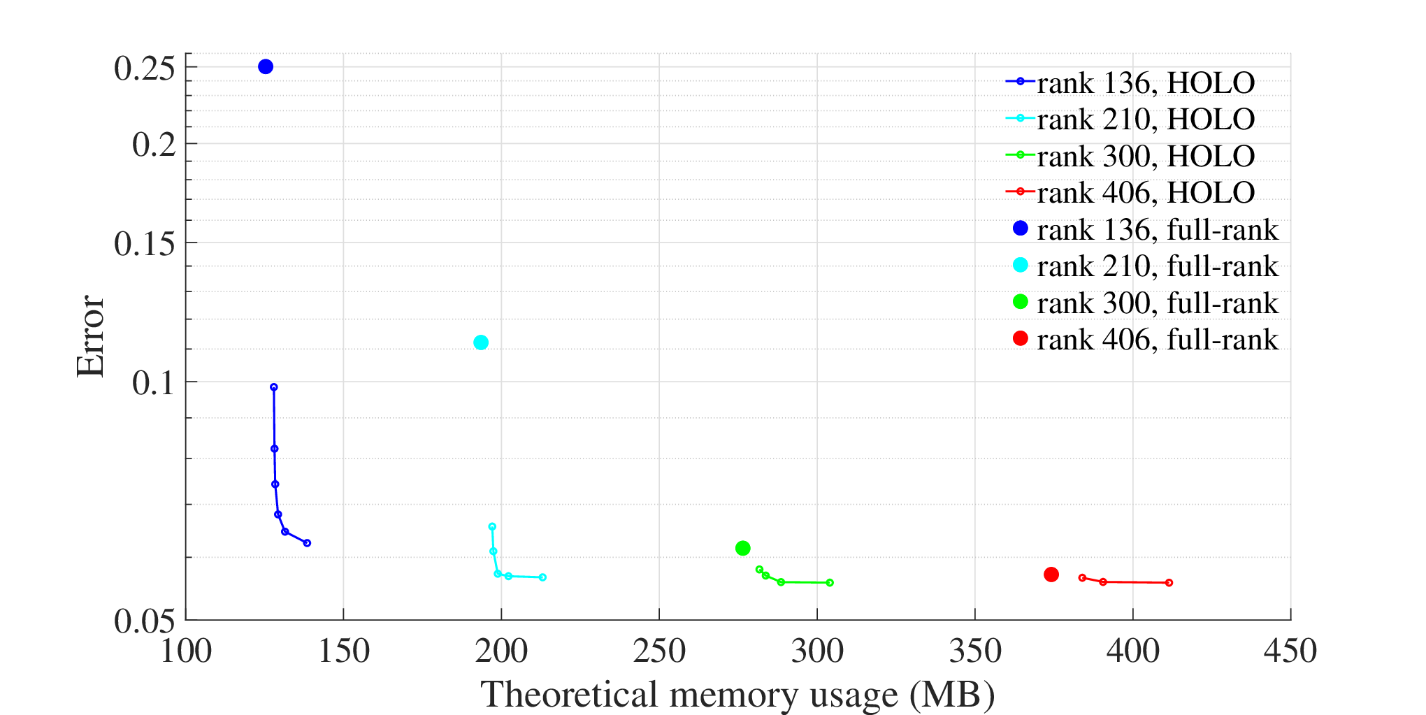
Figure 7 gives quantitative comparison, where we compare the root mean squares between the numerical solutions for the scalar flux and the analytic solution. It is apparent from the figure that the low-rank solution is more accurate than the full-rank solution with the same rank, which enables the choice to save memory or increase the accuracy. For example, the memory usage in full rank $P_{23}$ and $P_{39}$ with rank 300 are almost the same, as shown in the green line, but the accuracy is very different, as shown in Figure 6. Additionally, the rightmost dot of the dark blue line indicates that we can achieve an error of $0.06$ with memory $140$ MB; this accuracy cannot be obtained with less than $280$ MB in a full rank calculation, as shown in the large green dot. To demonstrate that the formulation in Eqs. (27) and (26) are correct representations of the required memory in practice, we measure the running memory in MATLAB with the “memory" function, as shown in Figure 8. From this figure, we observe that our estimates are valid.

The computational cost of the HOLO algorithm is presented in Figure 9. We notice that the running time and the memory of the HOLO solutions are much lower than the full rank P₅₉ and P₉₉ solutions. For example, the HOLO solution with P₉₉ and rank 300 requires 200 MB memory and 7s running time each time step, while the full rank P₉₉ solution needs 5000 MB and 65s, respectively. Note that our results have the error decrease stagnate because we have reduced the angular error in the solution to be smaller than the spatial discretization error, as shown in Figure 7. We also observe that the HOLO solution requires a longer running time than the classical full rank solution with the same rank due to the fact that the low-rank method has more arithmetic operations [45]. This indicates that to get the most benefit from a low-rank, HOLO approach, one should run the highest order in angle solution possible.

5.4 Hohlraum problem

We consider a modified Hohlraum problem [71] detailed in Figure 10. There is an isotopic source of $Q=1$ in the leftmost zone that is turned on at t = 0. The blank areas are dense materials with $\sigma_{t}=100\ \mathrm{cm^{-1}}$ and $\sigma_{s}=1\ \mathrm{cm^{-1}}$ , the blank area are purely scattering materials with $\sigma_{s}=\sigma_{t}=0.1\ \mathrm{cm^{-1}}$ . The high-fidelity $P_{141}$ solution is given in Figure 10. The spatial grid is set to be $130\times 130$ for the computational domain $[0,1.3]\times[0,1.3]$ . The simulation time is 2.6s and the CFL number is chosen to be 0.2.

In this test, we compare the P₃₉ HOLO solutions to the full rank solutions with the same rank. From Figure 10, we can see that the shape of particle distribution behind the first dense wall should be a triangle. But none of the full rank solutions can capture it, as shown in Figure 11, 11, 11 and 11. In contrast, the HOLO solution with only rank 3 can preserve this feature, while the rank 36 is nearly identical to the benchmark except for the area behind the second obstacle. Note that rank 36 is considered a small rank for this problem: for the full rank P₃₉ corresponds to $n=r=820$ and P₁₄₁ has $n=r=10153$ . In such a low-rank solution we cannot guarantee that the symmetries we expect in this problem (e.g., top/bottom symmetry) will be preserved by the projections. This is especially obvious on the logarithmic scale of Figure 11.

Figure 12 shows the deviation of the HOLO solutions of P₃₉ and the full rank solutions ranging from P₁ to P₁₅ to the full rank P₃₉. We observe that the HOLO solution is more accurate than the full rank solution with the same memory usage and converges to the high-order full rank solution faster.

5.5 Lattice problem

Next, we solve a $7\ cm\times 7\ cm$ checkerboard problem as shown in Figure 13. The spatial grid is $210\times 210$ . We run the simulations to $t=3.2$ s with $\mathrm{CFL}=0.2$ . Figure 14 shows the $P_{39}$ solutions with different rank. From Figure 14, we can see that the rank 210 solution is nearly identical to the full-rank solutions (a reduction of nearly a factor of 4). There are noticeable negative scalar flux regions in solutions with small rank, which is plotted in grey, as can be seen from Figure 14, 14 and 14. Specifically, the correct propagation speed is lost in the solution with rank 36, which is also shown in Figure 15. Therefore, we conclude that rank 36 is not sufficient for this problem.

5.6 Double Chevron problem

We use an asymmetric double chevron problem detailed in Figure 16 as our final benchmark. Numerical solutions at t = 0.9 s are computed using a $90\times 90$ spatial grid with a CFL number of 0.2. This problem was originally designed so that $m\approx n$ to get the largest possible benefit of the dynamic low-rank method. In this test, we compare the HOLO solutions of P₉₉ to the rank 5050, full rank P₉₉ solution. From Figure 17, we can see that the solution with rank 300 is close to the full rank solution over a range of 6 orders of magnitude in this problem, while the rank 36 and 78 solutions cannot capture the particle distribution behind the second chevron. By calculating the memory using (26) and (27), we find that $93\%$ of the memory can be saved by applying the HOLO algorithm with rank 300.

6 Conclusions

We have presented a HOLO algorithm to overcome the conservation issues in the dynamical low-rank method for radiative transfer. The key idea is to use the low-rank results to calculate the closure term of a two-moment system. When combined with a discontinuous Galerkin scheme we obtain a method that preserves the diffusion limit. These two improvements go a long way to making the method robust enough for a variety of physics applications.

Our methods use explicit time integration techniques to advance the solution in time. Future work should incorporate implicit time discretization techniques, perhaps similar to those recently developed to remove the backwards-in-time substep of the DLR method [72]. Additionally, other transport models (e.g., discrete ordinates) and energy-dependent problems should be fruitful areas of future research.

References

[1] Y. Azmy, E. Sartori, Nuclear computational science: A century in review, Springer Netherlands, 2010.
[2] G. Rybicki, A. Lightman, Radiative processes in astrophysics, Wiley-Interscience, 1985.
[3] A. D. Kim, M. Moscoso, Radiative transfer computations for optical beams, Journal of Computational Physics 185 (1) (2003) 50 – 60.
[4] G. L. Olson, L. H. Auer, M. L. Hall, Diffusion, P1 , and other approximate forms of radiation transport, Journal of Quantitative Spectroscopy and Radiative Transfer 64 (6) (1999) 619–634.
[5] J. E. Morel, Diffusion-limit asymptotics of the transport equation, the P_1/3 equations, and two flux-limited diffusion theories, Journal of Quantitative Spectroscopy and Radiative Transfer 65 (5) (2000) 769–778.
[6] C. D. Levermore, G. C. Pomraning, A flux-limited diffusion theory, The Astrophysical Journal 248 (1981) 321–334.
[7] D. S. Kershaw, Flux Limiting Nature’s Own Way - A New Method for Numerical Solution of the Transport Equation, Tech. Rep. UCRL-78378, Lawrence Livermore National Laboratory (LLNL), Livermore, CA (1976).
[8] T. A. Brunner, J. Paul Holloway, One-dimensional Riemann solvers and the maximum entropy closure, Journal of Quantitative Spectroscopy and Radiative Transfer 69 (5) (2001) 543–566.
[9] G. C. Pomraning, The equations of radiation hydrodynamics, Courier Corporation, 2005.
[10] S. I. Heizler, Asymptotic telegrapher’s equation (P₁) approximation for the transport equation, Nuclear science and engineering 166 (1) (2010) 17–35.
[11] R. G. McClarren, J. P. Holloway, T. A. Brunner, On solutions to the P_n equations for thermal radiative transfer, Journal of Computational Physics 227 (5) (2008) 2864–2885.
[12] R. G. McClarren, C. D. Hauck, Simulating radiative transfer with filtered spherical harmonics, Physics Letters A 374 (22) (2010) 2290–2296.
[13] R. G. McClarren, C. D. Hauck, Robust and accurate filtered spherical harmonics expansions for radiative transfer, Journal of Computational Physics 229 (16) (2010) 5597–5614.
[14] D. Radice, E. Abdikamalov, L. Rezzolla, C. D. Ott, A new spherical harmonics scheme for multi-dimensional radiation transport I. Static matter configurations, Journal of Computational Physics 242 (2013) 648–669.
[15] V. M. Laboure, R. G. McClarren, C. D. Hauck, Implicit filtered P_N for high-energy density thermal radiation transport using discontinuous Galerkin finite elements, Journal of Computational Physics 321 (2016) 624–643.
[16] G. N. Minerbo, Maximum entropy Eddington factors, Journal of Quantitative Spectroscopy and Radiative Transfer 20 (6) (1978) 541–545.
[17] E. Olbrant, C. D. Hauck, M. Frank, A realizability-preserving discontinuous Galerkin method for the M₁ model of radiative transfer, Journal of Computational Physics 231 (17) (2012) 5612–5639.
[18] W. Zheng, R. G. McClarren, Moment closures based on minimizing the residual of the P_N angular expansion in radiation transport, Journal of Computational Physics 314 (2016) 682–699.
[19] C. D. Levermore, Relating Eddington Factors to Flux Limiters, Journal of Quantitative Spectroscopy and Radiative Transfer 31 (2) (1984) 149–160.
[20] M. P. Laiu, C. D. Hauck, R. G. McClarren, D. P. O’Leary, A. L. Tits, Positive filtered P_n moment closures for linear kinetic equations, SIAM Journal on Numerical Analysis 54 (6) (2016) 3214–3238.
[21] R. G. McClarren, Theoretical aspects of the simplified Pn equations, Transport Theory and Statistical Physics 39 (2-4) (2010) 73–109.
[22] G. C. Pomraning, Asymptotic and variational derivations of the simplified P_N equations, Annals of nuclear energy 20 (9) (1993) 623–637.
[23] Y. Zhang, J. E. Morel, J. C. Ragusa, Convergence behavior of second-order transport equations in near-void problems, Journal of Quantitative Spectroscopy and Radiative Transfer 244 (2020) 106843.
[24] A. Buchan, C. Pain, M. Eaton, R. Smedley-Stevenson, A. Goddard, Linear and quadratic octahedral wavelets on the sphere for angular discretisations of the Boltzmann transport equation, Annals of Nuclear Energy 32 (11) (2005) 1224–1273.
[25] S. Dargaville, A. G. Buchan, R. P. Smedley-Stevenson, P. N. Smith, C. C. Pain, Scalable angular adaptivity for Boltzmann transport, Journal of Computational Physics 406 (2020) 109124.
[26] L. Soucasse, S. Dargaville, A. G. Buchan, C. C. Pain, A goal-based angular adaptivity method for thermal radiation modelling in non grey media, Journal of Quantitative Spectroscopy and Radiative Transfer 200 (2017) 215–224.
[27] J. C. Stone, Adaptive discrete-ordinates algorithms and strategies, Ph.D. thesis, Texas A&M University (2008).
[28] J. J. Jarrell, M. L. Adams, Discrete-ordinates quadrature sets based on linear discontinuous finite elements.
[29] C. Y. Lau, M. L. Adams, Discrete ordinates quadratures based on linear and quadratic discontinuous finite elements over spherical quadrilaterals, Nuclear Science and Engineering 185 (1) (2017) 36–52.
[30] E. Lewis, W. Miller, Computational Methods of Neutron Transport, John Wiley and Sons, 1984.
[31] J. Morel, J. McGhee, A self-adjoint angular flux equation, Nuclear Science and Engineering 132 (3) (1999) 312–325.
[32] C. Drumm, W. Fan, A. Bielen, J. Chenhall, Least-squares finite-element algorithms in the SCEPTRE radiation transport code, in: International Conference on Mathematics and Computational Methods Applied to Nuclear Science and Engineering (M&C 2011), 2011.
[33] J. Hansen, J. Peterson, J. Morel, J. Ragusa, Y. Wang, A Least-Squares Transport Equation Compatible with Voids, Journal of Computational and Theoretical Transport 43 (1-7) (2015) 374–401.
[34] C. Latimer, J. Kópházi, M. Eaton, R. McClarren, Spatial adaptivity of the saaf and weighted least squares (WLS) forms of the neutron transport equation using constraint based, locally refined, isogeometric analysis (IGA) with dual weighted residual (DWR) error measures, Journal of Computational Physics (2020) 109941.
[35] C. Latimer, J. Kópházi, M. Eaton, R. McClarren, A geometry conforming isogeometric method for the self-adjoint angular flux (SAAF) form of the neutron transport equation with a discrete ordinate (SN) angular discretisation, Annals of Nuclear Energy 136 (2020) 107049.
[36] Y. Wang, H. Zhang, R. C. Martineau, Diffusion acceleration schemes for self-adjoint angular flux formulation with a void treatment, Nuclear Science and Engineering 176 (2) (2014) 201–225.
[37] V. M. Laboure, R. G. McClarren, Y. Wang, Globally conservative, hybrid self-adjoint angular flux and least-squares method compatible with voids, Nuclear Science and Engineering 185 (2) (2017) 294–306.
[38] W. Zheng, R. G. McClarren, J. E. Morel, An accurate globally conservative subdomain discontinuous least-squares scheme for solving neutron transport problems, Nuclear Science and Engineering 189 (3) (2018) 259–271.
[39] J. C. Ragusa, Y. Wang, A two-mesh adaptive mesh refinement technique for sn neutral-particle transport using a higher-order DGFEM, Journal of computational and applied mathematics 233 (12) (2010) 3178–3188.
[40] B. Turcksin, J. C. Ragusa, W. Bangerth, Goal-oriented h-adaptivity for the multigroup SP_N equations, Nuclear Science and Engineering 165 (3) (2010) 305–319.
[41] Y. Wang, J. C. Ragusa, Standard and goal-oriented adaptive mesh refinement applied to radiation transport on 2D unstructured triangular meshes, Journal of Computational Physics 230 (3) (2011) 763–788.
[42] M. Hanuš, R. McClarren, On the use of symmetrized transport equation in goal-oriented adaptivity, Journal of Computational and Theoretical Transport 45 (4) (2016) 314–333.
[43] J. Kópházi, D. Lathouwers, A space–angle DGFEM approach for the Boltzmann radiation transport equation with local angular refinement, Journal of Computational Physics 297 (2015) 637–668.
[44] Z. Sun, C. D. Hauck, Low-memory, discrete ordinates, discontinuous Galerkin methods for radiative transport (2019). arXiv:1907.01027.
[45] Z. Peng, R. G. McClarren, M. Frank, A low-rank method for two-dimensional time-dependent radiation transport calculations, Journal of Computational Physics 421 (2020) 109735. doi:https://doi.org/10.1016/j.jcp.2020.109735.
[46] C. Lubich, From Quantum to Classical Molecular Dynamics: Reduced Models and Numerical Analysis (Zurich Lectures in Advanced Mathematics), European Mathematical Society, 2008.
[47] O. Koch, C. Lubich, Dynamical Low-Rank Approximation, SIAM Journal on Matrix Analysis and Applications 29 (2) (2007) 434–454.
[48] A. Nonnenmacher, C. Lubich, Dynamical low-rank approximation: applications and numerical experiments, Mathematics and Computers in Simulation 79 (4) (2008) 1346–1357. doi:10.1016/j.matcom.2008.03.007.
[49] O. Koch, C. Lubich, Dynamical Tensor Approximation, SIAM Journal on Matrix Analysis and Applications 31 (5) (2010) 2360–2375.
[50] E. Kieri, C. Lubich, H. Walach, Discretized dynamical low-rank approximation in the presence of small singular values, SIAM Journal on Numerical Analysis 54 (2) (2016) 1020–1038.
[51] C. Lubich, I. V. Oseledets, A projector-splitting integrator for dynamical low-rank approximation, BIT Numerical Mathematics 54 (1) (2014) 171–188. doi:10.1007/s10543-013-0454-0.
[52] C. Lubich, B. Vandereycken, H. Walach, Time integration of rank-constrained tucker tensors, SIAM Journal on Numerical Analysis 56 (3) (2018) 1273–1290. doi:10.1137/17M1146889.
[53] L. Einkemmer, C. Lubich, A Low-Rank Projector-Splitting Integrator for the Vlasov–Poisson Equation, SIAM Journal on Scientific Computing 40 (5) (2018) B1330–B1360.
[54] L. Einkemmer, A low-rank algorithm for weakly compressible flow, SIAM Journal on Scientific Computing 41 (5) (2019) A2795–A2814.
[55] L. Einkemmer, A. Ostermann, C. Piazzola, A low-rank projector-splitting integrator for the vlasov–maxwell equations with divergence correction, Journal of Computational Physics 403 (2020) 109063.
[56] L. Einkemmer, C. Lubich, A low-rank projector-splitting integrator for the vlasov–poisson equation, SIAM Journal on Scientific Computing 40 (5) (2018) B1330–B1360.
[57] L. Chacon, G. Chen, D. A. Knoll, C. Newman, H. Park, W. Taitano, J. A. Willert, G. Womeldorff, Multiscale high-order/low-order (HOLO) algorithms and applications, Journal of Computational Physics 330 (2017) 21–45.
[58] S. R. Bolding, A High-Order Low-Order Algorithm With Exponentially-Convergent Monte Carlo For Thermal Radiative Transfer Problems, Ph.D. thesis, Texas A&M University (2017).
[59] V. Y. Gol’din, A quasi-diffusion method of solving the kinetic equation, USSR Computational Mathematics and Mathematical Physics 4 (6) (1964) 136–149. doi:10.1016/0041-5553(64)90085-0.
[60] D. Y. Anistratov, Consistent spatial approximation of the low-order quasi-diffusion equations on coarse grids, Nuclear science and engineering 149 (2) (2005) 138–161.
[61] E. W. Larsen, J. E. Morel, W. F. Miller Jr, Asymptotic solutions of numerical transport problems in optically thick, diffusive regimes, Journal of Computational Physics 69 (2) (1987) 283–324.
[62] E. Larsen, J. Morel, Asymptotic solutions of numerical transport problems in optically thick, diffusive regimes ii, Journal of Computational Physics 83 (1) (1989) 212–236.
[63] D. Mihalas, Stellar Atmospheres, W.H. Freeman & Co, 1978.
[64] P. N. Brown, D. E. Shumaker, C. S. Woodward, Fully implicit solution of large-scale non-equilibrium radiation diffusion with high order time integration, Journal of Computational Physics 204 (2) (2005) 760–783.
[65] R. G. McClarren, R. B. Lowrie, The effects of slope limiting on asymptotic-preserving numerical methods for hyperbolic conservation laws, Journal of Computational Physics 227 (23) (2008) 9711–9726.
[66] R. P. Smedley-Stevenson, R. G. McClarren, Asymptotic diffusion limit of cell temperature discretisation schemes for thermal radiation transport, Journal of Computational Physics 286 (2015) 214–235.
[67] R. McClarren, J. P. Holloway, T. A. Brunner, Establishing an Asymptotic Diffusion Limit for Riemann Solvers on the Time-Dependent Equations, in: International Topical Meeting on Mathematics and Computation, Supercomputing, Reactor Physics and Nuclear and Biological Applications, American Nuclear Society, Avignon, France, 2005.
[68] B. D. Ganapol, P. McKenty, K. Peddicord, The generation of time-dependent neutron transport solutions in infinite media, Nuclear Science and Engineering 64 (2) (1977) 317–331.
[69] B. Ganapol, R. S. Baker, J. A. Dahl, R. E. Alcouffe, Homogeneous infinite media time-dependent analytical benchmarks, Tech. rep., Los Alamos National Laboratory (2001).
[70] B. D. Ganapol, Analytical Benchmarks for Nuclear Engineering Applications, Organisation for Economic Co-Operation and Development, 2008.
[71] C. D. Hauck, R. G. McClarren, A Collision-Based Hybrid Method for Time-Dependent, Linear, Kinetic Transport Equations, Multiscale Modeling and Simulation 11 (4) (2013) 1197–1227.
[72] G. Ceruti, C. Lubich, An unconventional robust integrator for dynamical low-rank approximation (2020). arXiv:2010.02022.