Rank-Based Testing
for Semiparametric VAR Models:
a measure transportation approach

M. Hallin,^(a) D. La Vecchia,^(b) and H. Liu^(c)
^(a)ECARES, Université libre de Bruxelles CP 114/4
Avenue F.D. Roosevelt 50 - B-1050 Bruxelles, Belgium
Email: mhallin@ulb.ac.be
^(b)Research Center for Statistics, University of Geneva
Boulevard du Pont d’Arve 40 - CH-1211 Geneva, Switzerland
Email: davide.lavecchia@unige.ch
^(c)Department of Mathematics and Statistics, Lancaster University
LA1 4YF Lancaster, UK
Email: h.liu11@lancaster.ac.uk

Abstract

We develop a class of tests for semiparametric vector autoregressive (VAR) models with unspecified innovation densities, based on the recent measure-transportation-based concepts of multivariate center-outward ranks and signs. We show that these concepts, combined with Le Cam’s asymptotic theory of statistical experiments, yield novel testing procedures, which (a) are valid under a broad class of innovation densities (possibly non-elliptical, skewed, and/or with infinite moments), (b) are optimal (locally asymptotically maximin or most stringent) at selected ones, and (c) are robust against additive outliers. In order to do so, we establish a Hájek asymptotic representation result, of independent interest, for a general class of center-outward rank-based serial statistics. As an illustration, we consider the problems of testing the absence of serial correlation in multiple-output and possibly non-linear regression (an extension of the classical Durbin-Watson problem) and the sequential identification of the order $p$ of a vector autoregressive (VAR( $p$ )) model. A Monte Carlo comparative study of our tests and their routinely-applied Gaussian competitors demonstrates the benefits (in terms of size, power, and robustness) of our methodology; these benefits are particularly significant in the presence of asymmetric and leptokurtic innovation densities. A real data application concludes the paper.

Keywords: Multivariate ranks, Distribution-freeness, Hájek representation, Local asymptotic normality, Durbin-Watson, VAR order identification.

1 Introduction

Despite the overwhelming empirical evidence, in most real-life datasets, of non-Gaussian and non-symmetric (non-elliptical) distributions, multivariate time series analysis remains very deeply marked by explicit or implicit Gaussian assumptions: correlogram-based and spectral methods, pseudo-Gaussian tests, Gaussian quasi-likelihoods, and their possible robustifications, are ubiquitous in methodological developments as well as in daily practice.

The theoretical justification for this prevalence of Gaussian methods looks quite solid at first sight and is seldom questioned: Gaussian quasi-likelihood methods are asymptotically valid (viz., pseudo-Gaussian tests have correct asymptotic nominal size and Gaussian quasi-maximum-likelihood estimators (QMLEs) are root- $n$ consistent) under a broad range $\mathcal{F}$ of non-Gaussian innovation densities $f$ (typically, under finite fourth-order moments).

A closer look at this asymptotic validity argument, however, reveals a fundamental weakness: while it holds, pointwise, for any given $f\in{\mathcal{F}}$ , it fails to hold uniformly over $\mathcal{F}$ . Consider, for instance, the sequence $\phi^{(n)}$ of Gaussian level- $\alpha$ tests rejecting a null hypothesis of the form $\mbox{\boldmath$\theta$}=\mbox{\boldmath$\theta$}_{0}$ whenever some test statistic $S^{(n)}$ exceeds the standard normal quantile $z_{\alpha}$ of order $(1-\alpha)$ . Denoting by ${\rm P}^{(n)}_{\mbox{\boldmath$\theta$},f}$ the distribution of the observation under parameter value $\theta$ and innovation density $f\in{\mathcal{F}}$ , assume that $\phi^{(n)}$ is a valid pseudo-Gaussian test at asymptotic level $\alpha$ , that is, satisfies

\lim_{n\to\infty}{\rm P}^{(n)}_{\mbox{\boldmath$\theta$}_{0},f}\left[S^{(n)}>z_{\alpha}\right]\leq\alpha

(1.1)

for any $f\in\mathcal{F}$ . This, however, is not sufficient if $f$ remains unspecified. The null, then, is the semiparametric hypothesis $\big\{{\rm P}^{(n)}_{\mbox{\boldmath$\theta$},f}|\,\mbox{\boldmath$\theta$}=\mbox{\boldmath$\theta$}_{0},\,f\in\mathcal{F}\big\}$ and, in order for $\phi^{(n)}$ to qualify as an asymptotically valid level- $\alpha$ test, the stronger condition

\lim_{n\to\infty}\sup_{f\in\mathcal{F}}{\rm P}^{(n)}_{\mbox{\boldmath$\theta$}_{0},f}\left[S^{(n)}>z_{\alpha}\right]\leq\alpha

(1.2)

which, in general, does not follow from (1.1), is required.

This lack of uniformity in the asymptotics of pseudo-Gaussian procedures is not just a mathematical detail: in the context of VAR estimation, Hallin et al., 2019 have shown that, depending on the actual innovation density $f$ , the finite-sample performance of a valid QMLE, for given sample size $n$ , can be extremely far from its asymptotic performance. That discrepancy between finite-sample and asymptotic performance is particularly significant (see the motivating example in the introduction of the same reference) in the presence of non-elliptical innovation densities such as mixture or skewed densities—a type of innovation distribution which is likely to occur in the case of omitted variables or covariates—and only gets worse as the dimension of the observation space increases. The same phenomenon is bound to take place in testing problems.

A remedy to this lack of uniformity of pseudo-Gaussian asymptotics is distribution-freeness. If indeed the test statistic $S^{(n)}$ is distribution-free under $\big\{{\rm P}^{(n)}_{\mbox{\boldmath$\theta$},f}|\,\mbox{\boldmath$\theta$}\in{\mbox{\boldmath$\Theta$}}_{0},\,f\in\mathcal{F}\big\}$ , then (1.1) and (1.2) are equivalent. Rank-based inference then naturally enters the picture: it follows indeed from Basu’s classical theorems on the relation between minimal sufficiency and distribution-freeness (see Appendix E in Hallin et al., 2020a or Chapters 5 and 10 in Lehmann and Romano, 2005) that, in the univariate case, the $\sigma$ -field generated by residual ranks is essentially¹¹ 1 That is, maximal up to $\mathcal{F}$ -null sets. maximal ancillary—intuitively, “maximal distribution-free".

Moreover, it follows from Hallin and Werker, 2003 that the semiparametric efficiency bounds at given density $f\in{\mathcal{F}}$ —which, for ARMA models, coincide with the parametric ones—can be reached by rank-based tests: normal-score (van der Waerden) rank tests in ARMA models, in particular, are achieving, under Gaussian $f$ , the same asymptotic performance as the (pseudo-)Gaussian ones while doing strictly and uniformly better under non-Gaussian $f$ (Hallin, 1994). Pseudo-Gaussian tests, thus, are not admissible and uniformly dominated by their normal-score rank-based counterparts.

All this, which strongly suggests abandoning pseudo-Gaussian methods in favor of rank-based ones, unfortunately, until recently was limited to univariate ARMA models due to the lack of an adequate multivariate extension of the univariate concept of ranks. Many proposals have been made in the literature—see Hallin et al., 2020a for a commented bibliography. None of them, however, is enjoying distribution-freeness—let alone maximal ancillarity—except for the so-called Mahalanobis ranks and signs (Hallin and Paindaveine, 2002; Hallin and Paindaveine, 2004a) under the quite restrictive assumption, however, of elliptical symmetry. This lack of a satisfactory concept of multivariate ranks has been dealt with recently with the introduction of the measure-transportation-based Monge-Kantorovich (Chernozhukov et al., 2017) and center-outward (Hallin, 2017) ranks and signs, the maximal ancillarity of which is established in Hallin et al., 2020a. Building on that concept, Hallin et al., 2020b are proposing distribution-free center-outward rank-based tests for multiple-output regression and MANOVA models, Ghosal and Sen, 2019 for goodness-of-fit, Deb and Sen, 2019 and Shi et al., 2020 for independence between vectors, while Hallin et al., 2019 are constructing center-outward R-estimators for VARMA models. The finite-sample performance of the new rank-based methods in all cases appears to be quite remarkable. In this paper, we similarly study a class of center-outward rank-based testing procedures for VAR models and illustrate their role in the problem of sequential VAR order selection (see Pötscher 1983) in the presence of unspecified innovation density.

The paper is organized as follows. Section 2 introduces notation and recalls some methodological facts about local asymptotic normality for VARs (Section 2.2) and the measure-transportation approach to center-outward ranks and signs (Section 2.3). Section 3 contains the main theoretical result of this paper: a Hájek representation theorem for serial statistics based on center-outward ranks and signs. This key result, of independent interest, extends to general scores the spherical-score result of Hallin et al., 2019, as well as the univariate results of Hallin et al., 1985 and Hallin and Vermandele, 1996. Based on LAN and the Hájek representation of Section 3, Section 4 introduces the notion of rank-based central sequence from which the rank-based test statistics are constructed in Section 5. Focusing on two particular problems, we develop, in Section 5.1, a rank-based extension of the classical Durbin-Watson procedure to multiple-output and possibly non-linear regression and, in Section 5.2 a sequential rank-based procedure for VAR order identification. Section 6 derives the Gaussian counterparts of the tests developed in Section 5 while Section 7 presents a Monte Carlo investigation of the finite-sample performance of the rank-based methods we are proposing (Sections 7.1 and 7.2) and concludes with a real-data application (Section 7.3).

2 Methodological background

Our approach is combining two basic methodological ingredients:

(a)

the local asymptotic normality of VAR models, as established in Garel and Hallin, 1995 and Hallin and Paindaveine, 2004a; the explicit statement (Section 2.2 and Proposition 2.1) of this property (with closed-form expressions²² 2 The difficulty in the derivation of these closed forms mainly stems from the fact that the VAR order $p_{0}$ under the null hypothesis can be strictly less than the order $p$ under the alternative. for central sequences and information matrices) requires some algebraic preparation, which is provided Appendix A and can be skipped at first reading;
(b)

the recently proposed (Chernozhukov et al., 2017; Hallin, 2017; Hallin et al., 2020a) measure-transportation-based concepts of multivariate center-outward ranks and signs: see Section 2.3 for precise definitions .

In this section, we first settle the notation (Section 2.1) before turning (Sections 2.2 and 2.3) to (a) and (b).

2.1 Notation and general setting

Consider the $d$ -dimensional VAR model of order $p\leq p_{1}$

{\mbox{\boldmath$A$}}_{\mbox{\boldmath$\theta$}}(L){\mbox{\boldmath$X$}}_{t}:=({\mbox{\boldmath$I$}}_{d}-\sum_{i=1}^{p_{1}}{\mbox{\boldmath$A$}}_{i}L^{i}){\mbox{\boldmath$X$}}_{t}=\mbox{\boldmath$\epsilon$}_{t},\quad t\in\mathbb{Z},

(2.1)

where ${\mbox{\boldmath$I$}}_{d}$ is the $d\times d$ identity matrix, ${\mbox{\boldmath$A$}}_{1},\ldots,{\mbox{\boldmath$A$}}_{p_{1}}$ are $d\times d$ matrix coefficients, $L$ is the lag operator, $\{\mbox{\boldmath$\epsilon$}_{t};t\in{\mathbb{Z}}\}$ is an i.i.d. innovation process with mean $0$ and probability density $f$ , and $\mbox{\boldmath$\theta$}:=((\text{vec}{{\mbox{\boldmath$A$}}_{1}})^{\prime},\ldots,(\text{vec}{{\mbox{\boldmath$A$}}_{p_{1}}})^{\prime})^{\prime}$ denotes the $({p_{1}}d^{2})$ -dimensional vector of autoregressive parameters. For $\theta$ of the form

\mbox{\boldmath$\theta$}_{0}:=((\text{vec}{{\mbox{\boldmath$A$}}_{1}})^{\prime},\ldots,(\text{vec}{{\mbox{\boldmath$A$}}_{p_{0}}})^{\prime},{\mbox{\boldmath$0$}}_{d^{2}(p_{1}-p_{0})\times 1}^{\prime})^{\prime}

(2.2)

(with $0<p_{0}<p_{1}$ ), ${\mbox{\boldmath$A$}}_{\mbox{\boldmath$\theta$}}(L)$ is the VAR operator

{\mbox{\boldmath$A$}}_{\mbox{\boldmath$\theta$}_{0}}(L)={\mbox{\boldmath$I$}}_{d}-\sum_{i=1}^{p_{0}}{\mbox{\boldmath$A$}}_{i}L^{i}

(2.3)

of order $p_{0}<p_{1}$ . For $p_{0}=0$ , (2.2), with $\mbox{\boldmath$\theta$}_{0}=(0,\ldots,0)$ yields the white noise model ${\mbox{\boldmath$X$}}_{t}=\mbox{\boldmath$\epsilon$}_{t}$ .

Denote by $\Theta$ the set of parameter values $\mbox{\boldmath$\theta$}\in\mathbb{R}^{{p_{1}}d^{2}}$ such that all solutions of the determinantal equation $\text{\rm det}\left({\mbox{\boldmath$A$}}_{\mbox{\boldmath$\theta$}}(z)\right)=0$ , $z\in\mathbb{C}$ lie outside the unit ball (the standard VAR stationarity condition) and by ${\mbox{\boldmath$\Theta$}}_{0}$ the set of parameter values $\mbox{\boldmath$\theta$}_{0}\in{\mbox{\boldmath$\Theta$}}$ of the form (2.2) with $|{\mbox{\boldmath$A$}}_{p_{0}}|\neq 0$ . The notation ${\mbox{\boldmath$A$}}_{0}(L)$ will be used for a null VAR $(p_{0})$ operator of the form (2.3) with unspecified $\mbox{\boldmath$\theta$}_{0}\in{\mbox{\boldmath$\Theta$}}_{0}$ , the notation ${\mbox{\boldmath$A$}}_{1}(L)$ for an alternative VAR $(p)$ operator ${\mbox{\boldmath$A$}}_{\mbox{\boldmath$\theta$}_{1}}(L)$ of order $p$ , that is, with unspecified $\mbox{\boldmath$\theta$}_{1}\in{\mbox{\boldmath$\Theta$}}$ and ${\mbox{\boldmath$A$}}_{p}\neq{\bf 0}$ for some $p_{0}\penalty\ \!<\penalty\ \!p\leq\penalty\ \!p_{1}$ . Denoting by ${\mbox{\boldmath$X$}}^{(n)}:=\{{\mbox{\boldmath$X$}}^{(n)}_{1},\ldots,{\mbox{\boldmath$X$}}^{(n)}_{n}\}$ (superscript ⁽ⁿ⁾ omitted whenever possible) an observed triangular array of solutions of (2.1), our objective is to construct rank-based tests of (a) the null hypothesis ${\mathcal{H}}^{(n)}_{\mbox{\boldmath$\theta$}_{0}}$ under which ${\mbox{\boldmath$X$}}^{(n)}$ was generated by a VAR operator of the form ${\mbox{\boldmath$A$}}_{\mbox{\boldmath$\theta$}_{0}}(L)$ (specified ${\mbox{\boldmath$\theta$}_{0}}\in{\mbox{\boldmath$\Theta$}}_{0}$ , unspecified innovation density) and (b) the null hypothesis ${\mathcal{H}}^{(n)}_{0}$ under which ${\mbox{\boldmath$X$}}^{(n)}$ was generated by a VAR operator of the form ${\mbox{\boldmath$A$}}_{0}(L)$ (unspecified ${\mbox{\boldmath$\theta$}_{0}}\in{\mbox{\boldmath$\Theta$}}_{0}$ , unspecified innovation density) against the alternative of a VAR operator of the form ${\mbox{\boldmath$A$}}_{1}(L)$ (unspecified $\mbox{\boldmath$\theta$}_{1}\in{\mbox{\boldmath$\Theta$}}_{1}$ , unspecified innovation density). The sequential order identification procedure then consists of performing such tests for $p_{0}=0,1,...$ and $p_{1}=p_{0}+1$ until the null hypothesis ${\mathcal{H}}^{(n)}_{0}$ no longer gets rejected.

2.2 Local asymptotic normality

In this section, we state the local asymptotic normality (LAN) result on which the construction of our tests heavily relies. LAN, of course, requires some regularity assumptions on $f$ ; we throughout assume the following (essentially borrowed from Garel and Hallin, 1995).

Assumption 1.

(i)

The innovation density $f$ belongs to the class $\mathcal{F}_{d}$ of non-vanishing (with respect to the Lebesgue measure $\mu_{d}$ on ${\mathbb{R}}^{d}$ ) densities³³ 3 The requirement that $f$ has support $\mathbb{R}^{d}$ can be relaxed to a requirement of a convex support (see del Barrio et al., 2020) at the expense, however, of a less direct definition of center-outward distribution and quantile functions. For the sake of simplicity, we are sticking to the assumption made here. i.e., for all $c\in{\mathbb{R}}^{+}\!$ , there exist $b_{c;f}$ and $a_{c;f}$ in $\mathbb{R}$ such that $0<b_{c;f}\leq a_{c;f}<\infty$ and $b_{c;f}\leq f({\mbox{\boldmath$x$}})\leq a_{c;f}$ for any $\|{\mbox{\boldmath$x$}}\|\leq c$ ;
(ii)

$\displaystyle{\int{\mbox{\boldmath$x$}}f({\mbox{\boldmath$x$}})\mathrm{d}\mu={\mbox{\boldmath$0$}}}$ and $\displaystyle{\int{\mbox{\boldmath$x$}}{\mbox{\boldmath$x$}}^{\prime}f({\mbox{\boldmath$x$}})\mathrm{d}\mu=\mbox{\boldmath$\Xi$}}$ where $\Xi$ is positive definite;
(iii)

$f^{1/2}$ is mean-square differentiable with mean-square gradient ${\mbox{\boldmath$D$}}f^{1/2}$ , that is, there exists a square-integrable vector ${\mbox{\boldmath$D$}}f^{1/2}$ such that, for all sequence ${\mbox{\boldmath$h$}}\in\mathbb{R}^{d}$ suchthat ${\mbox{\boldmath$0$}}\neq{\mbox{\boldmath$h$}}\rightarrow{\mbox{\boldmath$0$}}$ , $\displaystyle{({\mbox{\boldmath$h$}}^{\prime}{\mbox{\boldmath$h$}})^{-1}\int\left[f^{1/2}({\mbox{\boldmath$x$}}+{\mbox{\boldmath$h$}})-f^{1/2}({\mbox{\boldmath$x$}})-{\mbox{\boldmath$h$}}^{\prime}{\mbox{\boldmath$D$}}f^{1/2}({\mbox{\boldmath$x$}})\right]^{2}\mathrm{d}\mu\rightarrow 0;}$
(iv)

letting (the location score function) $\mbox{\boldmath$\varphi$}_{f}({\mbox{\boldmath$x$}}):=(\varphi_{1}({\mbox{\boldmath$x$}}),\ldots,\varphi_{d}({\mbox{\boldmath$x$}}))^{\prime}:=-2({\mbox{\boldmath$D$}}f^{1/2})/f^{1/2}$ ,

$\int[\varphi_{i}({\mbox{\boldmath$x$}})]^{4}f({\mbox{\boldmath$x$}})\mathrm{d}\mu<\infty,\ i=1,\ldots,d;$
(v)

the function ${\mbox{\boldmath$x$}}\mapsto\mbox{\boldmath$\varphi$}_{f}({\mbox{\boldmath$x$}})$ is piecewise Lipschitz, i.e., there exists a finite measurable partition of ${\mathbb{R}}^{d}$ into $J$ non-overlapping subsets $I_{1},\ldots,I_{J}$ such that, for all ${\mbox{\boldmath$x$}},{\mbox{\boldmath$y$}}$ in $I_{j}$ , $j=1,\ldots,J$ , $\|\mbox{\boldmath$\varphi$}_{f}({\mbox{\boldmath$x$}})-\mbox{\boldmath$\varphi$}_{f}({\mbox{\boldmath$y$}})\|\leq K\|{\mbox{\boldmath$x$}}-{\mbox{\boldmath$y$}}\|$ .

Denote by ${\mathcal{F}}_{d}^{*}$ the family of innovation densities satisfying Assumption 1.

Let ${\mbox{\boldmath$Z$}}_{1}^{(n)}(\mbox{\boldmath$\theta$}_{0}),\ldots,{\mbox{\boldmath$Z$}}_{n}^{(n)}(\mbox{\boldmath$\theta$}_{0})$ with ${\mbox{\boldmath$Z$}}_{t}^{(n)}(\mbox{\boldmath$\theta$}_{0}):={\mbox{\boldmath$A$}}_{\mbox{\boldmath$\theta$}_{0}}(L){\mbox{\boldmath$X$}}^{(n)}_{t}$ denote the residuals computed from the initial values ${\mbox{\boldmath$X$}}_{-p+1},\ldots,{\mbox{\boldmath$X$}}_{0}$ , the parameter value $\mbox{\boldmath$\theta$}_{0}$ , and the observations ${\mbox{\boldmath$X$}}^{(n)}$ . Clearly, ${\mbox{\boldmath$X$}}^{(n)}$ is the finite realization of a solution of (2.3) with parameter value $\mbox{\boldmath$\theta$}_{0}$ iff the residuals ${\mbox{\boldmath$Z$}}^{(n)}_{1}(\mbox{\boldmath$\theta$}_{0}),\ldots,{\mbox{\boldmath$Z$}}^{(n)}_{n}(\mbox{\boldmath$\theta$}_{0})$ and $\mbox{\boldmath$\epsilon$}_{1},\ldots,\mbox{\boldmath$\epsilon$}_{n}$ coincide. Denoting by ${\rm P}^{(n)}_{\mbox{\boldmath$\theta$}_{0};f}$ the distribution of ${\mbox{\boldmath$X$}}^{(n)}$ under parameter value $\mbox{\boldmath$\theta$}_{0}$ and innovation density $f$ , the residuals ${\mbox{\boldmath$Z$}}_{1}^{(n)}(\mbox{\boldmath$\theta$}_{0}),\ldots,{\mbox{\boldmath$Z$}}_{n}^{(n)}(\mbox{\boldmath$\theta$}_{0})$ under ${\rm P}^{(n)}_{\mbox{\boldmath$\theta$}_{0};f}$ thus are i.i.d. with density $f$ .

Write $L^{(n)}_{\mbox{\boldmath$\theta$}_{0}+n^{-1/2}{\mbox{\boldmath$\tau$}}^{(n)}/\mbox{\boldmath$\theta$}_{0};f}$ for the log-likelihood ratio $\log{\rm d}{\rm P}^{(n)}_{\mbox{\boldmath$\theta$}_{0}+n^{-1/2}{\mbox{\boldmath$\tau$}}^{(n)};f}/{\rm d}{\rm P}^{(n)}_{\mbox{\boldmath$\theta$}_{0};f}$ , where ${\mbox{\boldmath$\tau$}}^{(n)}$ is a bounded sequence of $\mathbb{R}^{p_{1}d^{2}}$ . Define

\mbox{\boldmath$\Delta$}^{(n)}_{f}(\mbox{\boldmath$\theta$}_{0}):=n^{1/2}{\mbox{\boldmath$M$}}_{\mbox{\boldmath$\theta$}_{0}}^{\prime}{\mbox{\boldmath$P$}}_{\mbox{\boldmath$\theta$}_{0}}^{\prime}{\mbox{\boldmath$Q$}}_{\mbox{\boldmath$\theta$}_{0}}^{(n)\prime}\mbox{\boldmath$\Gamma$}_{f}^{(n)}(\mbox{\boldmath$\theta$}_{0}),

(2.4)

where ${\mbox{\boldmath$M$}}_{\mbox{\boldmath$\theta$}_{0}}$ , ${\mbox{\boldmath$P$}}_{\mbox{\boldmath$\theta$}_{0}}$ , and ${\mbox{\boldmath$Q$}}^{(n)}_{\mbox{\boldmath$\theta$}_{0}}$ are given in Appendix A ((A.1) and (A.2)) and

\mbox{\boldmath$\Gamma$}_{f}^{(n)}(\mbox{\boldmath$\theta$}_{0}):=n^{-1/2}\left((n-1)^{1/2}(\text{vec}{\mbox{\boldmath$\Gamma$}_{1,f}^{(n)}(\mbox{\boldmath$\theta$}_{0})})^{\prime},\ldots,(n-i)^{1/2}(\text{vec}{\mbox{\boldmath$\Gamma$}_{i,f}^{(n)}(\mbox{\boldmath$\theta$}_{0})})^{\prime},\ldots,(\text{vec}{\mbox{\boldmath$\Gamma$}_{n-1,f}^{(n)}(\mbox{\boldmath$\theta$}_{0})})^{\prime}\right)^{\prime},

(2.5)

with the so-called $f$ -cross-covariance matrices

\mbox{\boldmath$\Gamma$}_{i,f}^{(n)}(\mbox{\boldmath$\theta$}_{0}):=(n-i)^{-1}\sum_{t=i+1}^{n}\mbox{\boldmath$\varphi$}_{f}({\mbox{\boldmath$Z$}}_{t}^{(n)}(\mbox{\boldmath$\theta$}_{0})){\mbox{\boldmath$Z$}}_{t-i}^{(n)\prime}(\mbox{\boldmath$\theta$}_{0}).

(2.6)

Finally, let

\mbox{\boldmath$\Lambda$}_{f}(\mbox{\boldmath$\theta$}_{0}):={\mbox{\boldmath$M$}}_{\mbox{\boldmath$\theta$}_{0}}^{\prime}{\mbox{\boldmath$P$}}_{\mbox{\boldmath$\theta$}_{0}}^{\prime}\underset{n\rightarrow\infty}{\lim}\left\{{\mbox{\boldmath$Q$}}_{\mbox{\boldmath$\theta$}_{0}}^{(n)\prime}[{\mbox{\boldmath$I$}}_{n-1}\otimes(\mbox{\boldmath$\Xi$}\otimes\mathbfcal{I}(f))]{\mbox{\boldmath$Q$}}_{\mbox{\boldmath$\theta$}_{0}}^{(n)}\right\}{\mbox{\boldmath$P$}}_{\mbox{\boldmath$\theta$}_{0}}{\mbox{\boldmath$M$}}_{\mbox{\boldmath$\theta$}_{0}}.

We then have the following LAN result (Hallin et al., 2019).

Proposition 2.1.

Let Assumption 1 hold. Then, for any $\mbox{\boldmath$\theta$}_{0}\in{\mbox{\boldmath$\Theta$}}_{0}$ and any bounded sequence ${\mbox{\boldmath$\tau$}}^{(n)}$ in ${\mathbb{R}}^{p_{1}d^{2}}\!$ , under ${\rm P}^{(n)}_{\mbox{\boldmath$\theta$}_{0};f}$ , as $n\rightarrow\infty$ ,

L^{(n)}_{\mbox{\boldmath$\theta$}_{0}+n^{-1/2}{\mbox{\boldmath$\tau$}}^{(n)}/\mbox{\boldmath$\theta$}_{0};f}={\mbox{\boldmath$\tau$}}^{{(n)}\prime}\mbox{\boldmath$\Delta$}^{(n)}_{f}(\mbox{\boldmath$\theta$}_{0})-\frac{1}{2}{\mbox{\boldmath$\tau$}}^{(n)\prime}\mbox{\boldmath$\Lambda$}_{f}(\mbox{\boldmath$\theta$}_{0}){\mbox{\boldmath$\tau$}}^{(n)}+o_{\rm P}(1),

(2.7)

and $\mbox{\boldmath$\Delta$}^{(n)}_{f}(\mbox{\boldmath$\theta$}_{0})\rightarrow{\mathcal{N}}({\mbox{\boldmath$0$}},\mbox{\boldmath$\Lambda$}_{f}(\mbox{\boldmath$\theta$}_{0})).$

Parametrically efficient (in the Hájek-Le Cam asymptotic sense) rank- and sign-based (hence, distribution-free) inference procedures in LAN families (with given $f$ ) are possible when the LAN central sequence (2.4) can be expressed in terms of signs and ranks. More precisely (a central sequence $\mbox{\boldmath$\Delta$}^{(n)}_{f}(\mbox{\boldmath$\theta$}_{0})$ is only defined up to $o_{{\rm P}}(1)$ -under- ${\rm P}^{(n)}_{\mbox{\boldmath$\theta$}_{0};f}$ terms), when there exists some $\utilde{\mbox{\boldmath$\Delta$}}^{(n)}_{f}(\mbox{\boldmath$\theta$}_{0})$ measurable with respects to the ranks and signs of the residuals ${\mbox{\boldmath$Z$}}^{(n)}_{t}(\mbox{\boldmath$\theta$}_{0})$ such that $\utilde{\mbox{\boldmath$\Delta$}}^{(n)}_{f}(\mbox{\boldmath$\theta$}_{0})-\mbox{\boldmath$\Delta$}^{(n)}_{f}(\mbox{\boldmath$\theta$}_{0})$ is $o_{{\rm P}}(1)$ under ${\rm P}^{(n)}_{\mbox{\boldmath$\theta$}_{0};f}$ as $n\to\infty$ .

In the univariate setting, this idea was exploited in Hallin and Puri, 1988; Hallin and Puri, 1991; Hallin and Puri, 1994, Hallin and Mélard, 1988, and Garel and Hallin, 1999, leading to a fairly complete toolbox of distribution-free procedures based on traditional ranks or signed ranks for ARMA models, in Benghabrit and Hallin, 1992; Benghabrit and Hallin, 1996 and Hallin and La Vecchia, 2017; Hallin and La Vecchia, 2020 for nonlinear time series models. In the multivariate context, under the assumption of ellipticity, Hallin and Paindaveine, 2002; Hallin and Paindaveine, 2005; Hallin and Paindaveine, 2006; Hallin and Paindaveine, 2008 for location, regression, and shape, Hallin et al., 2010; Hallin et al., 2013; Hallin et al., 2014 for principal and common principal components, andHallin and Paindaveine, 2004a; Hallin and Paindaveine, 2004b; Hallin and Paindaveine, 2005 for VAR and VARMA models, proposed test procedures based on the so-called Mahalanobis ranks and signs. However, the assumption of elliptic innovation density (which reduces to symmetry in the univariate case) severely restricts the applicability of these tests, specially in the analysis of economic data, where actual innovations, typically, are skewed and/or leptokurtic. Thus, with the aim of accommodating a more general and realistic setting of non-elliptical distribution, we develop here novel test procedures based on the notions of multivariate ranks and signs proposed by Chernozhukov et al., 2017 (under the name of Monge-Kantorovich ranks and signs) and developed in Hallin, 2017 and Hallin et al., 2020a under the name of center-outward ranks and signs. These new notions hinge on measure transportation theory; in their empirical version, they are based on the idea of an optimal coupling of the residuals $\{{\mbox{\boldmath$Z$}}^{(n)}_{t};1\leq t\leq n\}$ with a regular grid $\mathfrak{G}^{(n)}$ over the open unit ball ${\mathbb{S}}_{d}$ in $\mathbb{R}^{d}$ , which we now describe.

2.3 Center-outward ranks and signs

Let $\mathcal{P}_{d}$ denote the family of all distributions $\rm P$ with densities in ${\mathcal{F}}_{d}$ . For $\rm P$ in this family, the center-outward distribution functions defined below are continuous: see Hallin et al., 2020a. More general cases are studied in del Barrio et al., 2020, but require more cautious and less intuitive definitions which, for the sake of simplicity, we do not consider here. Denote by ${\rm U}_{d}$ the spherical uniform distribution over ${\mathbb{S}}_{d}$ , that is, the product of a uniform measure over the hypersphere ${\mathcal{S}}_{d-1}$ and a uniform over the unit interval of distances to the origin. The center-outward distribution function ${\mbox{\boldmath$F$}}_{{\mspace{-1mu}{\scriptscriptstyle\pm}}}$ of $\rm P$ is defined as the a.e. unique gradient of convex function mapping ${\mathbb{R}}^{d}$ to $\mathbb{S}_{d}$ and pushing $\rm P$ forward to ${\rm U}_{d}$ .⁴⁴ 4 That is, such that ${\mbox{\boldmath$F$}}_{{\mspace{-1mu}{\scriptscriptstyle\pm}}}({\bf X})\sim{\rm U}_{d}$ if ${\bf X}\sim{\rm P}.$ For ${\rm P}\in{\mathcal{P}}_{d}$ , such mapping is a homeomorphism between ${\mathbb{S}}_{d}\setminus\{{\bf 0}\}$ and $\mathbb{R}^{d}\setminus{\mbox{\boldmath$F$}}_{{\mspace{-1mu}{\scriptscriptstyle\pm}}}^{-1}(\{{\bf 0}\})$ (Figalli, 2018) and the corresponding center-outward quantile function is defined (letting, with a small abuse of notation, ${\mbox{\boldmath$Q$}}_{\mspace{-1mu}{\scriptscriptstyle\pm}}({\bf 0}):={\mbox{\boldmath$F$}}_{\mspace{-1mu}{\scriptscriptstyle\pm}}^{-1}(\{{\bf 0}\})$ ) as ${\mbox{\boldmath$Q$}}_{\mspace{-1mu}{\scriptscriptstyle\pm}}:={\mbox{\boldmath$F$}}_{\mspace{-1mu}{\scriptscriptstyle\pm}}^{-1}$ . For any given distribution $\rm P$ , ${\mbox{\boldmath$Q$}}_{{\mspace{-1mu}{\scriptscriptstyle\pm}}}$ induces a collection of continuous, connected, and nested quantile contours and regions; the center-outward median ${\mbox{\boldmath$Q$}}_{\mspace{-1mu}{\scriptscriptstyle\pm}}({\mbox{\boldmath$0$}})$ is a uniquely defined compact set of Lebesgue measure zero. We refer to Hallin et al., 2020a for details.

Turning to the sample, the residuals ${\mbox{\boldmath$Z$}}_{1}^{(n)}(\mbox{\boldmath$\theta$}_{0}),\ldots,{\mbox{\boldmath$Z$}}_{n}^{(n)}(\mbox{\boldmath$\theta$}_{0})$ under ${\rm P}^{(n)}_{\mbox{\boldmath$\theta$}_{0};f}$ are i.i.d. with density $f\in{\cal F}_{d}$ and center-outward distribution function ${\mbox{\boldmath$F$}}_{\pm}$ . For the empirical counterpart ${\mbox{\boldmath$F$}}^{(n)}_{\pm}$ of ${\mbox{\boldmath$F$}}_{\pm}$ , let $n$ factorize into $n=n_{R}n_{S}+n_{0},$ for $n_{R},n_{S},n_{0}\in\mathbb{N}$ and $0\leq n_{0}<\min\{n_{R},n_{S}\}$ , where $n_{R}\rightarrow\infty$ and $n_{S}\rightarrow\infty$ as $n\rightarrow\infty$ , and consider a sequence $\mathfrak{G}^{(n)}$ of grids, where each grid consists of the intersection between an $n_{S}$ -tuple $(\boldsymbol{u}_{1},\ldots\boldsymbol{u}_{n_{S}})$ of unit vectors, and the $n_{R}$ hyperspheres with radii $1/(n_{R}+1),\ldots,n_{R}/(n_{R}+1)$ centered at the origin, along with $n_{0}$ copies of the origin. The only requirement⁵⁵ 5 One exception will be made in the sequel when the so-called sign test scores are considered (see Section 5.3). Those scores being entirely based on directions, the grid can be constructed over the unit hypersphere rather than the unit ball, with an empirical distribution converging weakly to the uniform over the unit hypersphere. This is obtained by letting $n_{S}=n$ , $n_{R}=1$ , and $n_{0}=0$ . is that the sequence $\mathfrak{G}^{(n)}$ of grids is such that the discrete distribution with probability masses $1/n$ at each gridpoint and probability mass $n_{0}/n$ at the origin converges weakly to the uniform ${\rm U}_{d}$ over the ball $\mathbb{S}_{d}$ . Then, we define ${\mbox{\boldmath$F$}}_{\pm}^{(n)}({\mbox{\boldmath$Z$}}^{(n)}_{t})$ , for $t=1,\ldots,n$ as the solution (optimal mapping) of a coupling problem between the residuals and the grid. Specifically, the empirical center-outward distribution function is the (random) discrete mapping

{\mbox{\boldmath$F$}}^{(n)}_{\pm}:{\mbox{\boldmath$Z$}}^{(n)}:=({\mbox{\boldmath$Z$}}^{(n)}_{1},\ldots,{\mbox{\boldmath$Z$}}^{(n)}_{n})\mapsto({\mbox{\boldmath$F$}}^{(n)}_{\pm}({\mbox{\boldmath$Z$}}^{(n)}_{1}),\ldots,{\mbox{\boldmath$F$}}^{(n)}_{\pm}({\mbox{\boldmath$Z$}}^{(n)}_{n}))

satisfying

\sum_{t=1}^{n}\|{\mbox{\boldmath$Z$}}^{(n)}_{t}-{\mbox{\boldmath$F$}}^{(n)}_{\pm}({\mbox{\boldmath$Z$}}^{(n)}_{t})\|^{2}=\underset{T\in\mathcal{T}}{\min}\sum_{t=1}^{n}\|{\mbox{\boldmath$Z$}}^{(n)}_{t}-T({\mbox{\boldmath$Z$}}^{(n)}_{t})\|^{2},

(2.8)

where ${\mbox{\boldmath$Z$}}^{(n)}_{t}={\mbox{\boldmath$Z$}}^{(n)}_{t}(\mbox{\boldmath$\theta$})$ , the set $\{{\mbox{\boldmath$F$}}^{(n)}_{\pm}({\mbox{\boldmath$Z$}}^{(n)}_{t})|t=1,\ldots,n\}$ coincides with the $n$ points of the grid, $\|\cdot\|$ stands for the Euclidean norm, and $\mathcal{T}$ denotes the set of all possible bijective mappings between ${\mbox{\boldmath$Z$}}^{(n)}_{1},\ldots,{\mbox{\boldmath$Z$}}^{(n)}_{n}$ and the $n$ gridpoints.

Based on this empirical center-outward distribution function, the center-outward ranks are defined as

{R^{(n)}_{\pm,t}}:={R^{(n)}_{\pm,t}}(\mbox{\boldmath$\theta$}):=({n_{R}+1})\|{\mbox{\boldmath$F$}}^{(n)}_{\pm}({\mbox{\boldmath$Z$}}^{(n)}_{t})\|,

(2.9)

the center-outward signs as

{\mbox{\boldmath$S$}}^{(n)}_{\pm,t}:={{\mbox{\boldmath$S$}}^{(n)}_{\pm,t}}(\mbox{\boldmath$\theta$}):={\mbox{\boldmath$F$}}^{(n)}_{\pm}({\mbox{\boldmath$Z$}}^{(n)}_{t})I[{\mbox{\boldmath$F$}}^{(n)}_{\pm}({\mbox{\boldmath$Z$}}^{(n)}_{t})\neq\boldsymbol{0}]/\|{\mbox{\boldmath$F$}}^{(n)}_{\pm}({\mbox{\boldmath$Z$}}^{(n)}_{t})\|.

(2.10)

It follows that ${\mbox{\boldmath$F$}}^{(n)}_{\pm}({\mbox{\boldmath$Z$}}_{t}^{(n)})$ factorizes into

{\mbox{\boldmath$F$}}^{(n)}_{\pm}({\mbox{\boldmath$Z$}}_{t}^{(n)})=\frac{R^{(n)}_{\pm,t}}{n_{R}+1}{\mbox{\boldmath$S$}}^{(n)}_{\pm,t},\quad\text{ whence }\quad{\mbox{\boldmath$Z$}}_{t}^{(n)}={\mbox{\boldmath$Q$}}^{(n)}_{\pm}\Big(\frac{R^{(n)}_{\pm,t}}{n_{R}+1}{\mbox{\boldmath$S$}}^{(n)}_{\pm,t}\Big).

(2.11)

Those ranks and signs are jointly distribution-free (for $f\in{\cal F}_{d}$ ): more precisely, under ${\rm P}^{(n)}_{\mbox{\boldmath$\theta$}_{0};f}$ , the $n$ -tuple ${\mbox{\boldmath$F$}}^{(n)}_{\pm}({\mbox{\boldmath$Z$}}_{1}^{(n)}),\ldots,{\mbox{\boldmath$F$}}^{(n)}_{\pm}({\mbox{\boldmath$Z$}}_{n}^{(n)})$ is uniformly distributed over the $n!/n_{0}!$ permutations with repetition of the $n$ underlying gridpoints (the origin having multiplicity $n_{0}$ ). Moreover, the center-outward distribution functions, ranks, and signs inherit, from the invariance properties of Euclidean distances, elementary but remarkable invariance and equivariance properties: Hallin et al., 2020b show that center-outward quantities enjoy invariance/equivariance with respect to shift, global scale, and orthogonal transformations.

3 A Hájek asymptotic representation result for serial center-outward rank statistics

3.1 Hájek asymptotic representation

Throughout this section, denote by ${\mbox{\boldmath$F$}}_{\pm,t}:={\mbox{\boldmath$F$}}_{\pm}({\mbox{\boldmath$Z$}}_{t}^{(n)}(\mbox{\boldmath$\theta$}_{0}))$ the value of the center-outward distribution function ${\mbox{\boldmath$F$}}_{\pm}$ associated with innovation density $f$ computed at ${\mbox{\boldmath$Z$}}_{t}={\mbox{\boldmath$Z$}}_{t}^{(n)}(\mbox{\boldmath$\theta$}_{0})$ and by ${\mbox{\boldmath$F$}}_{\pm,t}^{(n)}:={\mbox{\boldmath$F$}}_{\pm}^{(n)}({\mbox{\boldmath$Z$}}_{t}^{(n)}(\mbox{\boldmath$\theta$}_{0}))$ its empirical counterpart computed from the $n$ -tuple of residuals ${\mbox{\boldmath$Z$}}_{1}^{(n)}(\mbox{\boldmath$\theta$}_{0}),\ldots,{\mbox{\boldmath$Z$}}_{n}^{(n)}(\mbox{\boldmath$\theta$}_{0})$ . Considering two score functions ${\mbox{\boldmath$J$}}_{1}$ and ${\mbox{\boldmath$J$}}_{2}$ from ${\mathbb{S}}_{d}$ to $\mathbb{R}^{d}$ , define, for $1\leq i\leq n-1,$

\hbox{\hskip 3.45831pt\hskip-3.45831pt\hbox{$\mbox{\boldmath$\Gamma$}$}\hskip-3.45831pt\hskip-4.09721pt\raisebox{-2.98203pt}{\hbox{$\scriptscriptstyle\thicksim$}}\hskip-4.09721pt\hskip 3.45831pt}_{i,{\mbox{\boldmath$J$}}_{1},{\mbox{\boldmath$J$}}_{2}}^{(n)}(\mbox{\boldmath$\theta$}_{0}):=(n-i)^{-1}\sum_{t=i+1}^{n}{\mbox{\boldmath$a$}}({\mbox{\boldmath$F$}}^{(n)}_{\pm,t},{\mbox{\boldmath$F$}}^{(n)}_{\pm,t-i})\vskip-5.69054pt

(3.1)

and

\underline{\mbox{\boldmath$\Gamma$}}_{i,{\mbox{\boldmath$J$}}_{1},{\mbox{\boldmath$J$}}_{2}}^{(n)}(\mbox{\boldmath$\theta$}_{0}):=(n-i)^{-1}\sum_{t=i+1}^{n}{\mbox{\boldmath$J$}}_{1}({\mbox{\boldmath$F$}}_{\pm,t}){\mbox{\boldmath$J$}}_{2}^{\prime}({\mbox{\boldmath$F$}}_{\pm,t-i}),\vskip-2.84526pt

(3.2)

where the function ${\mbox{\boldmath$a$}}:\mathbb{S}_{d}\times\mathbb{S}_{d}\rightarrow\mathbb{R}^{d^{2}}$ satisfies, under ${\rm P}^{(n)}_{\mbox{\boldmath$\theta$}_{0};f}$ ,

\lim_{n\rightarrow\infty}{\rm E}\left\|\text{vec}\left({\mbox{\boldmath$a$}}({\mbox{\boldmath$F$}}^{(n)}_{\pm,2},{\mbox{\boldmath$F$}}^{(n)}_{\pm,1})-{\mbox{\boldmath$J$}}_{1}({\mbox{\boldmath$F$}}_{\pm,2}){\mbox{\boldmath$J$}}_{2}^{\prime}({\mbox{\boldmath$F$}}_{\pm,1})\right)\right\|^{2}\rightarrow 0.\vskip-8.53581pt

(3.3)

Let

	$\displaystyle{\mbox{\boldmath$m$}}^{(n)}:=$	$\displaystyle{\rm E}_{{\mbox{\boldmath$\theta$}_{0}};f}[{\mbox{\boldmath$a$}}({\mbox{\boldmath$F$}}^{(n)}_{\pm,2},{\mbox{\boldmath$F$}}^{(n)}_{\pm,1})]$
	$\displaystyle=$	$\displaystyle\,[n(n-1)]^{-1}\Bigg[\sum_{\mathfrak{g}_{1}\neq\mathfrak{g}_{2}\in\mathfrak{G}^{(n)}\setminus{\bf 0}}\!\!\!\!{\mbox{\boldmath$a$}}(\mathfrak{g}_{2},\mathfrak{g}_{1})+n_{0}\!\!\!\!\sum_{\mathfrak{g}\in\mathfrak{G}^{(n)}\setminus{\bf 0}}\!\!\!\!{\mbox{\boldmath$a$}}(\mathfrak{g},{\bf 0})+n_{0}\!\!\!\!\sum_{\mathfrak{g}\in\mathfrak{G}^{(n)}\setminus{\bf 0}}\!\!\!\!{\mbox{\boldmath$a$}}({\bf 0},\mathfrak{g})+n_{0}(n_{0}-1){\mbox{\boldmath$a$}}({\bf 0},{\bf 0})\Bigg]$

and

\displaystyle{\mbox{\boldmath$m$}}:=

\displaystyle{\rm E}_{{\mbox{\boldmath$\theta$}_{0}};f}[{\mbox{\boldmath$J$}}_{1}({\mbox{\boldmath$F$}}_{\pm,2}){\mbox{\boldmath$J$}}_{2}^{\prime}({\mbox{\boldmath$F$}}_{\pm,1})]={\rm E}_{{\mbox{\boldmath$\theta$}_{0}};f}[{\mbox{\boldmath$J$}}_{1}({\mbox{\boldmath$F$}}_{\pm,1})]{\rm E}_{{\mbox{\boldmath$\theta$}_{0}};f}[{\mbox{\boldmath$J$}}_{2}^{\prime}({\mbox{\boldmath$F$}}_{\pm,1})],

where ${\rm E}_{{\mbox{\boldmath$\theta$}_{0}};f}$ denotes expectation under ${\rm P}^{(n)}_{\mbox{\boldmath$\theta$}_{0};f}$ . Clearly, ${\mbox{\boldmath$m$}}^{(n)}\!$ , which does not depend on $f$ , is centering $\hbox{\hskip 3.45831pt\hskip-3.45831pt\hbox{$\mbox{\boldmath$\Gamma$}$}\hskip-3.45831pt\hskip-4.09721pt\raisebox{-2.98203pt}{\hbox{$\scriptscriptstyle\thicksim$}}\hskip-4.09721pt\hskip 3.45831pt}_{i,{\mbox{\boldmath$J$}}_{1},{\mbox{\boldmath$J$}}_{2}}^{(n)}$ under the (null) hypothesis that $({\mbox{\boldmath$F$}}^{(n)}_{\pm,1},\ldots,{\mbox{\boldmath$F$}}^{(n)}_{\pm,n})$ is uniform over the permutations of the grid it was constructed from (that is, under any innovation density in $\mathcal{F}_{d}$ ), while ${\mbox{\boldmath$m$}}={\mbox{\boldmath$m$}}_{f}$ , which depends on $f$ through ${\mbox{\boldmath$F$}}_{\pm}$ , is centering $\underline{\mbox{\boldmath$\Gamma$}}_{i,{\mbox{\boldmath$J$}}_{1},{\mbox{\boldmath$J$}}_{2}}^{(n)}$ under ${\rm P}^{(n)}_{\mbox{\boldmath$\theta$}_{0};f}$ only; none of them depends on $i$ .

An essential step in Hájek’s approach to the asymptotics of univariate ranks is the so-called Hájek asymptotic representation of linear rank statistics which, contrary to earlier approaches based on empirical processes, allows for unbounded square-integrable score functions. Such results first were obtained (Hájek 1961; Hájek and Šidák 1967) for the nonserial rank statistics used in the context of linear models (single-output regression, ANOVA, etc.); Hallin et al. (1985) extend them to serial rank statistics—with scores involving several ranks at a time—appearing in the analysis of time-series models. The matrices $\hbox{\hskip 3.45831pt\hskip-3.45831pt\hbox{$\mbox{\boldmath$\Gamma$}$}\hskip-3.45831pt\hskip-4.09721pt\raisebox{-2.98203pt}{\hbox{$\scriptscriptstyle\thicksim$}}\hskip-4.09721pt\hskip 3.45831pt}_{i,{\mbox{\boldmath$J$}}_{1},{\mbox{\boldmath$J$}}_{2}}^{(n)}$ are of that serial type, hence require an extension of Hallin et al. (1985) and Hallin and Vermandele, 1996 (which only deal with classical “univariate ranks") to the present case of multivariate center-outward ranks and signs. Proposition 3.1 establishes such asymptotic representation for $\text{\rm vec}(\hbox{\hskip 3.45831pt\hskip-3.45831pt\hbox{$\mbox{\boldmath$\Gamma$}$}\hskip-3.45831pt\hskip-4.09721pt\raisebox{-2.98203pt}{\hbox{$\scriptscriptstyle\thicksim$}}\hskip-4.09721pt\hskip 3.45831pt}_{i,{\mbox{\boldmath$J$}}_{1},{\mbox{\boldmath$J$}}_{2}}^{(n)}(\mbox{\boldmath$\theta$}_{0})-{\mbox{\boldmath$m$}}^{(n)})$ under the following assumption on the score functions ${\mbox{\boldmath$J$}}_{1}$ and ${\mbox{\boldmath$J$}}_{2}$ .

Assumption 2.

(i) ${\mbox{\boldmath$J$}}_{1}$ and ${\mbox{\boldmath$J$}}_{2}$ are continuous over $\mathbb{S}_{d}$ ;
(ii) ${\mbox{\boldmath$J$}}_{1}$ and ${\mbox{\boldmath$J$}}_{2}$ are square-integrable, that is, $\int_{\mathbb{S}_{d}}\|{\mbox{\boldmath$J$}}_{\ell}({\mbox{\boldmath$u$}})\|^{2}{\rm dU}_{d}<\infty$ for $\ell=1,2$ , and, for any sequence $\mathfrak{s}^{(n)}:=\{{\bf s}_{1}^{(n)},\ldots,{\bf s}_{n}^{(n)}\}$ of $n$ -tuples in $\mathbb{S}_{d}$ such that the uniform discrete distribution over $\mathfrak{s}^{(n)}$ converges weakly to ${\rm U}_{d}$ as $n\rightarrow\infty$ ,

\underset{n\rightarrow\infty}{\lim}n^{-1}\sum_{t=1}^{n}\|{\mbox{\boldmath$J$}}_{\ell}({\bf s}_{t}^{(n)})\|^{2}=\int_{\mathbb{S}_{d}}\|{\mbox{\boldmath$J$}}_{\ell}({\mbox{\boldmath$u$}})\|^{2}{\rm dU}_{d},\quad\ell=1,2.

(3.4)

When ${\mbox{\boldmath$J$}}_{\ell}({{\mbox{\boldmath$u$}}})$ is of the form (spherical score) $J_{\ell}(\|{\mbox{\boldmath$u$}}\|)\frac{{\mbox{\boldmath$u$}}}{\|{\mbox{\boldmath$u$}}\|}$ with $J_{\ell}:[0,1)\to\mathbb{R}$ continuous, a sufficient condition for (3.4) is the traditional assumption of bounded variation (that is, $J_{\ell}$ is the continuous difference of two nondecreasing functions).

Proposition 3.1.

Let Assumption 2 hold. Then, for any positive integer $i$ ,

{\rm E}\left\|\text{\rm vec}\left(\hbox{\hskip 3.45831pt\hskip-3.45831pt\hbox{$\mbox{\boldmath$\Gamma$}$}\hskip-3.45831pt\hskip-4.09721pt\raisebox{-2.98203pt}{\hbox{$\scriptscriptstyle\thicksim$}}\hskip-4.09721pt\hskip 3.45831pt}_{i,{\mbox{\boldmath$J$}}_{1},{\mbox{\boldmath$J$}}_{2}}^{(n)}(\mbox{\boldmath$\theta$}_{0})-{\mbox{\boldmath$m$}}^{(n)}-\underline{\mbox{\boldmath$\Gamma$}}_{i,{\mbox{\boldmath$J$}}_{1},{\mbox{\boldmath$J$}}_{2}}^{(n)}(\mbox{\boldmath$\theta$}_{0})+{\mbox{\boldmath$m$}}\right)\right\|^{2}=o((n-i)^{-1/2})

under ${\rm P}^{(n)}_{\mbox{\boldmath$\theta$}_{0};f}$ (any $f\in{\cal F}_{d}$ ) and ${\rm P}^{(n)}_{{\mbox{\boldmath$\theta$}_{0}}+n^{-1/2}{\mbox{\boldmath$\tau$}};f}$ (any $f\in{\cal F}^{*}_{d}$ ), as $n\rightarrow\infty$ .

See Section Appendix B: Proofs of Proposition and Lemma for the proof.

Adopting Hájek’s terminology, examples of functions $a$ satisfying (3.3) for given ${\mbox{\boldmath$J$}}_{1}$ and ${\mbox{\boldmath$J$}}_{2}$ are the approximate scores

{\mbox{\boldmath$a$}}_{\rm a}({\mbox{\boldmath$F$}}^{(n)}_{\pm,t},{\mbox{\boldmath$F$}}^{(n)}_{\pm,s}):={\mbox{\boldmath$J$}}_{1}({\mbox{\boldmath$F$}}^{(n)}_{\pm,t}){\mbox{\boldmath$J$}}_{2}^{\prime}({\mbox{\boldmath$F$}}^{(n)}_{\pm,s})\vskip-2.84526pt

and (still with ${\rm E}_{{\mbox{\boldmath$\theta$}_{0}};f}$ denoting expectation under ${\rm P}^{(n)}_{\mbox{\boldmath$\theta$}_{0};f}$ ) the exact scores

{\mbox{\boldmath$a$}}_{\rm e}({\mbox{\boldmath$F$}}^{(n)}_{\pm,t},{\mbox{\boldmath$F$}}^{(n)}_{\pm,s}):={\rm E}_{{\mbox{\boldmath$\theta$}_{0}};f}\left[{\mbox{\boldmath$J$}}_{1}({\mbox{\boldmath$F$}}_{\pm,t}){\mbox{\boldmath$J$}}_{2}^{\prime}({\mbox{\boldmath$F$}}_{\pm,s})\big|{\mbox{\boldmath$F$}}^{(n)}_{\pm,t},{\mbox{\boldmath$F$}}^{(n)}_{\pm,s}\right].\vskip-2.84526pt

We then have, for ${\mbox{\boldmath$a$}}_{\rm a}$ and ${\mbox{\boldmath$a$}}_{\rm e}$ , the following lemma.

Lemma 3.1.

Let Assumption 2 hold. Put

\mbox{\boldmath$\xi$}_{t,s;{\rm a}}^{(n)}\!:=\text{\rm vec}({\mbox{\boldmath$a$}}_{\rm a}({\mbox{\boldmath$F$}}^{(n)}_{\pm,t},{\mbox{\boldmath$F$}}^{(n)}_{\pm,s})),\ \ \mbox{\boldmath$\xi$}_{t,s;{\rm e}}^{(n)}\!:=\text{\rm vec}({\mbox{\boldmath$a$}}_{\rm e}({\mbox{\boldmath$F$}}^{(n)}_{\pm,t},{\mbox{\boldmath$F$}}^{(n)}_{\pm,s})),\vskip-5.69054pt

and

\mbox{\boldmath$\xi$}_{t,s}\!:=\text{\rm vec}({\mbox{\boldmath$J$}}_{1}({\mbox{\boldmath$F$}}_{\pm,t}){\mbox{\boldmath$J$}}_{2}^{\prime}({\mbox{\boldmath$F$}}_{\pm,s})).

Then, under ${\rm P}^{(n)}_{\mbox{\boldmath$\theta$}_{0};f}$ (any $f\in{\cal F}_{d}$ ) and ${\rm P}^{(n)}_{\mbox{\boldmath$\theta$}_{0}+n^{-1/2}{\mbox{\boldmath$\tau$}};f}$ (any $f\in{\cal F}_{d}^{*}$ ),

{\rm E}\|\mbox{\boldmath$\xi$}_{2,1;{\rm a}}^{(n)}-\mbox{\boldmath$\xi$}_{2,1}\|^{2}\rightarrow 0\quad\text{and}\quad{\rm E}\|\mbox{\boldmath$\xi$}_{2,1;{\rm e}}^{(n)}-\mbox{\boldmath$\xi$}_{2,1}\|^{2}\rightarrow 0\quad\text{as $n\rightarrow\infty$. }

(3.5)

Letting

{\mbox{\boldmath$m$}}_{\rm a}^{(n)}:={\rm E}_{{\mbox{\boldmath$\theta$}_{0}};f}[{\mbox{\boldmath$a$}}_{\rm a}({\mbox{\boldmath$F$}}^{(n)}_{\pm,t},{\mbox{\boldmath$F$}}^{(n)}_{\pm,s})],\quad{\mbox{\boldmath$m$}}_{\rm e}^{(n)}:={\rm E}_{{\mbox{\boldmath$\theta$}_{0}};f}[{\mbox{\boldmath$a$}}_{\rm e}({\mbox{\boldmath$F$}}^{(n)}_{\pm,t},{\mbox{\boldmath$F$}}^{(n)}_{\pm,s})]\vskip-2.84526pt

and, for $1\leq i\leq n-1$ ,

\hbox{\hskip 3.45831pt\hskip-3.45831pt\hbox{$\mbox{\boldmath$\Gamma$}$}\hskip-3.45831pt\hskip-4.09721pt\raisebox{-2.98203pt}{\hbox{$\scriptscriptstyle\thicksim$}}\hskip-4.09721pt\hskip 3.45831pt}_{i;{\rm a}}^{(n)}(\mbox{\boldmath$\theta$}_{0}):=(n-i)^{-1}\sum_{t=i+1}^{n}{\mbox{\boldmath$a$}}_{\rm a}({\mbox{\boldmath$F$}}^{(n)}_{\pm,t},{\mbox{\boldmath$F$}}^{(n)}_{\pm,t-i})\vskip-5.69054pt

and

\hbox{\hskip 3.45831pt\hskip-3.45831pt\hbox{$\mbox{\boldmath$\Gamma$}$}\hskip-3.45831pt\hskip-4.09721pt\raisebox{-2.98203pt}{\hbox{$\scriptscriptstyle\thicksim$}}\hskip-4.09721pt\hskip 3.45831pt}_{i;{\rm e}}^{(n)}(\mbox{\boldmath$\theta$}_{0}):=(n-i)^{-1}\sum_{t=i+1}^{n}{\mbox{\boldmath$a$}}_{\rm e}({\mbox{\boldmath$F$}}^{(n)}_{\pm,t},{\mbox{\boldmath$F$}}^{(n)}_{\pm,t-i}),

the following proposition follows as a corollary to Proposition 3.1 and Lemma 3.1.

Proposition 3.2.

Let Assumption 2 hold. Then, for any positive integer $i$ ,

{(i)}\ {\rm E}\left\|(n-i)^{1/2}\text{\rm vec}(\hbox{\hskip 3.45831pt\hskip-3.45831pt\hbox{$\mbox{\boldmath$\Gamma$}$}\hskip-3.45831pt\hskip-4.09721pt\raisebox{-2.98203pt}{\hbox{$\scriptscriptstyle\thicksim$}}\hskip-4.09721pt\hskip 3.45831pt}_{i;{\rm a}}^{(n)}(\mbox{\boldmath$\theta$}_{0})-{\mbox{\boldmath$m$}}_{\rm a}^{(n)}-\underline{\mbox{\boldmath$\Gamma$}}_{i,{\mbox{\boldmath$J$}}_{1},{\mbox{\boldmath$J$}}_{2}}^{(n)}(\mbox{\boldmath$\theta$}_{0})+{\mbox{\boldmath$m$}})\right\|^{2}=o(1),

{(ii)}\ {\rm E}\left\|(n-i)^{1/2}\text{\rm vec}(\hbox{\hskip 3.45831pt\hskip-3.45831pt\hbox{$\mbox{\boldmath$\Gamma$}$}\hskip-3.45831pt\hskip-4.09721pt\raisebox{-2.98203pt}{\hbox{$\scriptscriptstyle\thicksim$}}\hskip-4.09721pt\hskip 3.45831pt}_{i;{\rm e}}^{(n)}(\mbox{\boldmath$\theta$}_{0})-{\mbox{\boldmath$m$}}_{\rm e}^{(n)}-\underline{\mbox{\boldmath$\Gamma$}}_{i,{\mbox{\boldmath$J$}}_{1},{\mbox{\boldmath$J$}}_{2}}^{(n)}(\mbox{\boldmath$\theta$}_{0})+{\mbox{\boldmath$m$}})\right\|^{2}=o(1),\vskip-2.84526pt

and, consequently,

{(iii)}\ {\rm E}\left\|(n-i)^{1/2}\text{\rm vec}(\hbox{\hskip 3.45831pt\hskip-3.45831pt\hbox{$\mbox{\boldmath$\Gamma$}$}\hskip-3.45831pt\hskip-4.09721pt\raisebox{-2.98203pt}{\hbox{$\scriptscriptstyle\thicksim$}}\hskip-4.09721pt\hskip 3.45831pt}_{i;{\rm a}}^{(n)}(\mbox{\boldmath$\theta$}_{0})-{\mbox{\boldmath$m$}}_{\rm a}^{(n)}-\hbox{\hskip 3.45831pt\hskip-3.45831pt\hbox{$\mbox{\boldmath$\Gamma$}$}\hskip-3.45831pt\hskip-4.09721pt\raisebox{-2.98203pt}{\hbox{$\scriptscriptstyle\thicksim$}}\hskip-4.09721pt\hskip 3.45831pt}_{i;{\rm e}}^{(n)}(\mbox{\boldmath$\theta$}_{0})+{\mbox{\boldmath$m$}}_{\rm e}^{(n)})\right\|^{2}=o(1)\vskip-2.84526pt

under ${\rm P}^{(n)}_{\mbox{\boldmath$\theta$}_{0};f}$ (any $f\in{\cal F}_{d}$ ) and ${\rm P}^{(n)}_{\mbox{\boldmath$\theta$}_{0}+n^{-1/2}{\mbox{\boldmath$\tau$}};f}$ (any $f\in{\cal F}_{d}^{*}$ ), as $n\rightarrow\infty$ .

Assume, without loss of generality, that ${\mbox{\boldmath$J$}}_{1}$ and ${\mbox{\boldmath$J$}}_{2}$ are such that ${\mbox{\boldmath$m$}}={\bf 0}$ (a sufficient condition is either $\int_{\mathbb{S}_{d}}{\mbox{\boldmath$J$}}_{1}({\mbox{\boldmath$u$}}){\rm dU}_{d}={\bf 0}$ or $\int_{\mathbb{S}_{d}}{\mbox{\boldmath$J$}}_{2}({\mbox{\boldmath$u$}}){\rm dU}_{d}={\bf 0}$ ). Then, for $d=\penalty\ \!1$ , ${\mbox{\boldmath$m$}}_{\rm a}^{(n)}$ and ${\mbox{\boldmath$m$}}_{\rm e}^{(n)}$ both are $o(n^{-1/2})$ (see Lemma 1 in Hallin and La Vecchia, 2017) and $m$ , ${\mbox{\boldmath$m$}}_{\rm a}^{(n)}$ , and ${\mbox{\boldmath$m$}}_{\rm e}^{(n)}$ can be omitted in Proposition 3.2. That simplification, however, is no longer valid when $d>1$ .

The proofs of Proposition 3.1 and Lemma 3.1 are given in Appendix B.

4 Center-outward rank-based central sequences

The basic idea underlying the construction of our rank-based tests is the definition of rank-based versions $\utilde{\mbox{\boldmath$\Delta$}}^{(n)}_{f}(\mbox{\boldmath$\theta$}_{0})$ of the central sequences $\mbox{\boldmath$\Delta$}^{(n)}_{f}(\mbox{\boldmath$\theta$}_{0})$ . Recall that $\utilde{\mbox{\boldmath$\Delta$}}^{(n)}_{f}(\mbox{\boldmath$\theta$}_{0})$ qualifies as a central sequence as soon as $\utilde{\mbox{\boldmath$\Delta$}}^{(n)}_{f}(\mbox{\boldmath$\theta$}_{0})-\mbox{\boldmath$\Delta$}^{(n)}_{f}(\mbox{\boldmath$\theta$}_{0})=o_{\rm P}(1)$ under ${\rm P}^{(n)}_{\mbox{\boldmath$\theta$}_{0};f}$ .

4.1 Construction and asymptotic representation

Writing ${\mbox{\boldmath$F$}}^{(n)}_{\pm,t}$ , $R^{(n)}_{\pm,t}$ and ${\mbox{\boldmath$S$}}^{(n)}_{\pm,t}$ for ${\mbox{\boldmath$F$}}^{(n)}_{\pm}({\mbox{\boldmath$Z$}}_{t}^{(n)}(\mbox{\boldmath$\theta$}_{0}))$ , ${R^{(n)}_{\pm,t}}(\mbox{\boldmath$\theta$}_{0})$ and ${{\mbox{\boldmath$S$}}^{(n)}_{\pm,t}}(\mbox{\boldmath$\theta$}_{0})$ , respectively, consider the center-outward rank-based counterpart of ${\mbox{\boldmath$\Gamma$}}^{(n)}_{f}(\mbox{\boldmath$\theta$}_{0})$ . Specifically, define

	$\displaystyle\hbox{\hskip 3.45831pt\hskip-3.45831pt\hbox{$\mbox{\boldmath$\Gamma$}$}\hskip-3.45831pt\hskip-4.09721pt\raisebox{-2.98203pt}{\hbox{$\scriptscriptstyle\thicksim$}}\hskip-4.09721pt\hskip 3.45831pt}_{{\mbox{\boldmath$J$}}_{1}{\mbox{\boldmath$J$}}_{2}}^{(n)}(\mbox{\boldmath$\theta$}_{0}):=$	$\displaystyle n^{-1/2}\left((n-1)^{1/2}(\text{vec}\,\hbox{\hskip 3.45831pt\hskip-3.45831pt\hbox{$\mbox{\boldmath$\Gamma$}$}\hskip-3.45831pt\hskip-4.09721pt\raisebox{-2.98203pt}{\hbox{$\scriptscriptstyle\thicksim$}}\hskip-4.09721pt\hskip 3.45831pt}_{1,{\mbox{\boldmath$J$}}_{1},{\mbox{\boldmath$J$}}_{2}}^{(n)}(\mbox{\boldmath$\theta$}_{0}))^{\prime},\ldots,\right.$
		$\displaystyle\qquad\left.(n-i)^{1/2}(\text{vec}\,\hbox{\hskip 3.45831pt\hskip-3.45831pt\hbox{$\mbox{\boldmath$\Gamma$}$}\hskip-3.45831pt\hskip-4.09721pt\raisebox{-2.98203pt}{\hbox{$\scriptscriptstyle\thicksim$}}\hskip-4.09721pt\hskip 3.45831pt}_{i,{\mbox{\boldmath$J$}}_{1},{\mbox{\boldmath$J$}}_{2}}^{(n)}(\mbox{\boldmath$\theta$}_{0}))^{\prime},\ldots,(\text{vec}\,\hbox{\hskip 3.45831pt\hskip-3.45831pt\hbox{$\mbox{\boldmath$\Gamma$}$}\hskip-3.45831pt\hskip-4.09721pt\raisebox{-2.98203pt}{\hbox{$\scriptscriptstyle\thicksim$}}\hskip-4.09721pt\hskip 3.45831pt}_{n-1,{\mbox{\boldmath$J$}}_{1},{\mbox{\boldmath$J$}}_{2}}^{(n)}(\mbox{\boldmath$\theta$}_{0}))^{\prime}\right)^{\prime},$		(4.1)

with

\hbox{\hskip 3.45831pt\hskip-3.45831pt\hbox{$\mbox{\boldmath$\Gamma$}$}\hskip-3.45831pt\hskip-4.09721pt\raisebox{-2.98203pt}{\hbox{$\scriptscriptstyle\thicksim$}}\hskip-4.09721pt\hskip 3.45831pt}_{i,{\mbox{\boldmath$J$}}_{1},{\mbox{\boldmath$J$}}_{2}}^{(n)}(\mbox{\boldmath$\theta$}_{0}):=(n-i)^{-1}\sum_{t=i+1}^{n}{\mbox{\boldmath$J$}}_{1}\left(\frac{R^{(n)}_{\pm,t}}{n_{R}+1}{\mbox{\boldmath$S$}}^{(n)}_{\pm,t}\right){\mbox{\boldmath$J$}}_{2}^{\prime}\left(\frac{R^{(n)}_{\pm,t-i}}{n_{R}+1}{\mbox{\boldmath$S$}}^{(n)}_{\pm,t-i}\right),\quad i=1,\ldots,n-1,

(4.2)

where ${\mbox{\boldmath$J$}}_{1}$ and ${\mbox{\boldmath$J$}}_{2}:{\mathcal{S}}_{d}\rightarrow{\mathbb{R}}$ are score functions satisfying Assumption 2. Call $\hbox{\hskip 3.45831pt\hskip-3.45831pt\hbox{$\mbox{\boldmath$\Gamma$}$}\hskip-3.45831pt\hskip-4.09721pt\raisebox{-2.98203pt}{\hbox{$\scriptscriptstyle\thicksim$}}\hskip-4.09721pt\hskip 3.45831pt}_{i,{\mbox{\boldmath$J$}}_{1},{\mbox{\boldmath$J$}}_{2}}^{(n)}(\mbox{\boldmath$\theta$}_{0})$ a (residual) lag- $i$ rank-based cross-covariance matrix. As an approximate-score rank-based statistic, $\hbox{\hskip 3.45831pt\hskip-3.45831pt\hbox{$\mbox{\boldmath$\Gamma$}$}\hskip-3.45831pt\hskip-4.09721pt\raisebox{-2.98203pt}{\hbox{$\scriptscriptstyle\thicksim$}}\hskip-4.09721pt\hskip 3.45831pt}_{i,{\mbox{\boldmath$J$}}_{1},{\mbox{\boldmath$J$}}_{2}}^{(n)}(\mbox{\boldmath$\theta$}_{0})$ under ${\rm P}^{(n)}_{\mbox{\boldmath$\theta$}_{0};f}$ has expectation

{\mbox{\boldmath$m$}}_{\rm a}^{(n)}={\rm E}_{{\mbox{\boldmath$\theta$}_{0}};f}\left[\hbox{\hskip 3.45831pt\hskip-3.45831pt\hbox{$\mbox{\boldmath$\Gamma$}$}\hskip-3.45831pt\hskip-4.09721pt\raisebox{-2.98203pt}{\hbox{$\scriptscriptstyle\thicksim$}}\hskip-4.09721pt\hskip 3.45831pt}_{i,{\mbox{\boldmath$J$}}_{1},{\mbox{\boldmath$J$}}_{2}}^{(n)}(\mbox{\boldmath$\theta$}_{0})\right]={\rm E}_{{\mbox{\boldmath$\theta$}_{0}};f}\left[{\mbox{\boldmath$J$}}_{1}({\mbox{\boldmath$F$}}^{(n)}_{\pm,2}){\mbox{\boldmath$J$}}_{2}^{\prime}({\mbox{\boldmath$F$}}^{(n)}_{\pm,1})\right]

under ${\rm P}^{(n)}_{\mbox{\boldmath$\theta$}_{0};f}$ , hence under any ${\rm P}^{(n)}_{\mbox{\boldmath$\theta$}_{0};g}$ , $g\in{\cal F}_{d}$ . We thus have

{\rm E}_{{\mbox{\boldmath$\theta$}_{0}};f}\left[\hbox{\hskip 3.45831pt\hskip-3.45831pt\hbox{$\mbox{\boldmath$\Gamma$}$}\hskip-3.45831pt\hskip-4.09721pt\raisebox{-2.98203pt}{\hbox{$\scriptscriptstyle\thicksim$}}\hskip-4.09721pt\hskip 3.45831pt}_{{\mbox{\boldmath$J$}}_{1}{\mbox{\boldmath$J$}}_{2}}^{(n)}(\mbox{\boldmath$\theta$}_{0})\right]=n^{-1/2}\left({\rm diag}((n-1)^{1/2},\ldots,(n-i)^{1/2},\ldots,1)\otimes{\mbox{\boldmath$I$}}_{d^{2}}\right)\,\text{vec}\,({\mbox{\boldmath$m$}}_{\rm a}^{(n)}).

(4.3)

Similarly define

	$\displaystyle\underline{\mbox{\boldmath$\Gamma$}}_{{\mbox{\boldmath$J$}}_{1}{\mbox{\boldmath$J$}}_{2}}^{(n)}(\mbox{\boldmath$\theta$}_{0}):=$	$\displaystyle n^{-1/2}\left((n-1)^{1/2}(\text{vec}\,\underline{\mbox{\boldmath$\Gamma$}}_{1,{\mbox{\boldmath$J$}}_{1},{\mbox{\boldmath$J$}}_{2}}^{(n)}(\mbox{\boldmath$\theta$}_{0}))^{\prime},\ldots,\right.$
		$\displaystyle\qquad\left.(n-i)^{1/2}(\text{vec}\,\underline{\mbox{\boldmath$\Gamma$}}_{i,{\mbox{\boldmath$J$}}_{1},{\mbox{\boldmath$J$}}_{2}}^{(n)}(\mbox{\boldmath$\theta$}_{0}))^{\prime},\ldots,(\text{vec}\,\underline{\mbox{\boldmath$\Gamma$}}_{n-1,{\mbox{\boldmath$J$}}_{1},{\mbox{\boldmath$J$}}_{2}}^{(n)}(\mbox{\boldmath$\theta$}_{0}))^{\prime}\right)^{\prime},$		(4.4)

with $\underline{\mbox{\boldmath$\Gamma$}}_{i,{\mbox{\boldmath$J$}}_{1},{\mbox{\boldmath$J$}}_{2}}^{(n)}(\mbox{\boldmath$\theta$}_{0})$ defined in (3.2). Clearly, $\underline{\mbox{\boldmath$\Gamma$}}_{{\mbox{\boldmath$J$}}_{1}{\mbox{\boldmath$J$}}_{2}}^{(n)}(\mbox{\boldmath$\theta$}_{0})$ is a counterpart of $\hbox{\hskip 3.45831pt\hskip-3.45831pt\hbox{$\mbox{\boldmath$\Gamma$}$}\hskip-3.45831pt\hskip-4.09721pt\raisebox{-2.98203pt}{\hbox{$\scriptscriptstyle\thicksim$}}\hskip-4.09721pt\hskip 3.45831pt}_{{\mbox{\boldmath$J$}}_{1}{\mbox{\boldmath$J$}}_{2}}^{(n)}(\mbox{\boldmath$\theta$}_{0})$ constructed from the center-outward distribution function and under ${\rm P}^{(n)}_{\mbox{\boldmath$\theta$}_{0};f}$ has mean

{\rm E}_{{\mbox{\boldmath$\theta$}_{0}};f}\left[\underline{\mbox{\boldmath$\Gamma$}}_{{\mbox{\boldmath$J$}}_{1}{\mbox{\boldmath$J$}}_{2}}^{(n)}(\mbox{\boldmath$\theta$}_{0})\right]=n^{-1/2}\left({\rm diag}((n-1)^{1/2},\ldots,(n-i)^{1/2},\ldots,1)\otimes{\mbox{\boldmath$I$}}_{d^{2}}\right)\,\text{vec}\,({\mbox{\boldmath$m$}})

Denote by $\utilde{\mbox{\boldmath$\Delta$}}^{(n)}_{{\mbox{\boldmath$J$}}_{1}{\mbox{\boldmath$J$}}_{2}}(\mbox{\boldmath$\theta$}_{0})$ and $\underline{\mbox{\boldmath$\Delta$}}^{(n)}_{{\mbox{\boldmath$J$}}_{1}{\mbox{\boldmath$J$}}_{2}}(\mbox{\boldmath$\theta$}_{0})$ the statistics resulting from substituting

\hbox{\hskip 3.45831pt\hskip-3.45831pt\hbox{$\mbox{\boldmath$\Gamma$}$}\hskip-3.45831pt\hskip-4.09721pt\raisebox{-2.98203pt}{\hbox{$\scriptscriptstyle\thicksim$}}\hskip-4.09721pt\hskip 3.45831pt}_{{\mbox{\boldmath$J$}}_{1}{\mbox{\boldmath$J$}}_{2}}^{(n)}(\mbox{\boldmath$\theta$}_{0})-{\rm E}_{{\mbox{\boldmath$\theta$}_{0}};f}\left[\hbox{\hskip 3.45831pt\hskip-3.45831pt\hbox{$\mbox{\boldmath$\Gamma$}$}\hskip-3.45831pt\hskip-4.09721pt\raisebox{-2.98203pt}{\hbox{$\scriptscriptstyle\thicksim$}}\hskip-4.09721pt\hskip 3.45831pt}_{{\mbox{\boldmath$J$}}_{1}{\mbox{\boldmath$J$}}_{2}}^{(n)}(\mbox{\boldmath$\theta$}_{0})\right]\quad\text{ and }\quad\underline{\mbox{\boldmath$\Gamma$}}_{{\mbox{\boldmath$J$}}_{1}{\mbox{\boldmath$J$}}_{2}}^{(n)}(\mbox{\boldmath$\theta$}_{0})-{\rm E}_{{\mbox{\boldmath$\theta$}_{0}};f}\left[\underline{\mbox{\boldmath$\Gamma$}}_{{\mbox{\boldmath$J$}}_{1}{\mbox{\boldmath$J$}}_{2}}^{(n)}(\mbox{\boldmath$\theta$}_{0})\right],\vskip-5.69054pt

respectively, for ${\mbox{\boldmath$\Gamma$}}_{f}^{(n)}(\mbox{\boldmath$\theta$}_{0})$ in the definition (2.4) of the central sequence $\mbox{\boldmath$\Delta$}^{(n)}_{f}(\mbox{\boldmath$\theta$}_{0})$ . For the scores ${\mbox{\boldmath$J$}}_{1}=\mbox{\boldmath$\varphi$}\circ{{\mbox{\boldmath$F$}}}_{\pm}^{-1}$ and ${\mbox{\boldmath$J$}}_{2}={{\mbox{\boldmath$F$}}}_{\pm}^{-1}$ , the following corollary to Proposition 3.2 (i) implies that $\utilde{\mbox{\boldmath$\Delta$}}^{(n)}_{{\mbox{\boldmath$J$}}_{1}{\mbox{\boldmath$J$}}_{2}}(\mbox{\boldmath$\theta$}_{0})$ is asymptotically equivalent, under ${\rm P}^{(n)}_{\mbox{\boldmath$\theta$}_{0};f}$ , to $\mbox{\boldmath$\Delta$}^{(n)}_{f}(\mbox{\boldmath$\theta$}_{0})$ , hence constitutes a rank-based version of the same central sequence. These scores depend on $f$ : if $f$ stands for the actual innovation density, thus, they are oracle scores. They can be computed, however, at any chosen reference density such as the spherical or skew Gaussian; see Section 5.3. With a slight abuse of terminology, irrespective of ${\mbox{\boldmath$J$}}_{1}$ and ${\mbox{\boldmath$J$}}_{2}$ , we therefore call $\utilde{\mbox{\boldmath$\Delta$}}^{(n)}_{{\mbox{\boldmath$J$}}_{1}{\mbox{\boldmath$J$}}_{2}}(\mbox{\boldmath$\theta$}_{0})$ a rank-based central sequence. Proposition 3.2 (iii) moreover implies that, asymptotically, $\utilde{\mbox{\boldmath$\Delta$}}^{(n)}_{{\mbox{\boldmath$J$}}_{1}{\mbox{\boldmath$J$}}_{2}}(\mbox{\boldmath$\theta$}_{0})$ is equivalent to the expectation of $\mbox{\boldmath$\Delta$}^{(n)}_{f}(\mbox{\boldmath$\theta$}_{0})$ conditional on the $\sigma$ -field generated by the center-outward ranks and signs—that is, the projection of $\mbox{\boldmath$\Delta$}^{(n)}_{f}(\mbox{\boldmath$\theta$}_{0})$ onto the space of center-outward ranks and signs. We thus can state the following corollary.

Corollary 4.1.

Let Assumption 2 hold. Then,

{\rm E}\left\|\utilde{\mbox{\boldmath$\Delta$}}^{(n)}_{{\mbox{\boldmath$J$}}_{1}{\mbox{\boldmath$J$}}_{2}}(\mbox{\boldmath$\theta$}_{0})-\underline{\mbox{\boldmath$\Delta$}}^{(n)}_{{\mbox{\boldmath$J$}}_{1}{\mbox{\boldmath$J$}}_{2}}(\mbox{\boldmath$\theta$}_{0})\right\|^{2}=o(1)

(4.5)

4.2 Asymptotic normality

The joint asymptotic normality of the statistics $(n-i)^{1/2}\text{\rm vec}(\hbox{\hskip 3.45831pt\hskip-3.45831pt\hbox{$\mbox{\boldmath$\Gamma$}$}\hskip-3.45831pt\hskip-4.09721pt\raisebox{-2.98203pt}{\hbox{$\scriptscriptstyle\thicksim$}}\hskip-4.09721pt\hskip 3.45831pt}_{i,{\mbox{\boldmath$J$}}_{1},{\mbox{\boldmath$J$}}_{2}}^{(n)}(\mbox{\boldmath$\theta$}_{0})-{\mbox{\boldmath$m$}}_{\rm a}^{(n)})$ and their asymptotic linearity, which entail the asymptotic normality and asymptotic linearity of $\utilde{\mbox{\boldmath$\Delta$}}^{(n)}_{{\mbox{\boldmath$J$}}_{1}{\mbox{\boldmath$J$}}_{2}}(\mbox{\boldmath$\theta$}_{0})$ , are essential in the construction of our rank-based tests. In view of the Hájek asymptotic representation result of Section 3, it is sufficient to derive these asymptotic results for $(n-i)^{1/2}\text{\rm vec}(\underline{\mbox{\boldmath$\Gamma$}}_{i,{\mbox{\boldmath$J$}}_{1},{\mbox{\boldmath$J$}}_{2}}^{(n)}(\mbox{\boldmath$\theta$}_{0})-{\mbox{\boldmath$m$}})$ .

Let

	$\displaystyle{{\mbox{\boldmath$C$}}}_{{\mbox{\boldmath$J$}}_{1}{\mbox{\boldmath$J$}}_{2}}:=$	$\displaystyle\int_{\mathbb{S}_{d}}({\mbox{\boldmath$I$}}_{d}\otimes{\mbox{\boldmath$J$}}_{1}({\mbox{\boldmath$u$}}_{1}))\left[\int_{\mathbb{S}_{d}}{\mbox{\boldmath$J$}}_{2}({\mbox{\boldmath$u$}}_{2}){\mbox{\boldmath$J$}}_{2}^{\prime}({\mbox{\boldmath$u$}}_{2}){\rm dU}_{d}({\mbox{\boldmath$u$}}_{2})\right]({\mbox{\boldmath$I$}}_{d}\otimes{\mbox{\boldmath$J$}}_{1}^{\prime}({\mbox{\boldmath$u$}}_{1})){\rm dU}_{d}({\mbox{\boldmath$u$}}_{1})$
		$\displaystyle-\Big({\mbox{\boldmath$I$}}_{d}\otimes\int_{\mathbb{S}_{d}}{\mbox{\boldmath$J$}}_{1}({\mbox{\boldmath$u$}}){\rm dU}_{d}\Big)\int_{\mathbb{S}_{d}}{\mbox{\boldmath$J$}}_{2}({\mbox{\boldmath$u$}}){\rm dU}_{d}\int_{\mathbb{S}_{d}}{\mbox{\boldmath$J$}}_{2}^{\prime}({\mbox{\boldmath$u$}}){\rm dU}_{d}\Big({\mbox{\boldmath$I$}}_{d}\otimes\int_{\mathbb{S}_{d}}{\mbox{\boldmath$J$}}_{1}^{\prime}({\mbox{\boldmath$u$}}){\rm dU}_{d}\Big)$

and

\displaystyle{\mbox{\boldmath$K$}}_{{\mbox{\boldmath$J$}}_{1},{\mbox{\boldmath$J$}}_{2},f}

\displaystyle:=\int_{\mathbb{S}_{d}}({\mbox{\boldmath$I$}}_{d}\otimes{\mbox{\boldmath$J$}}_{1}({\mbox{\boldmath$u$}}_{1}))\left[\int_{\mathbb{S}_{d}}{\mbox{\boldmath$J$}}_{2}({\mbox{\boldmath$u$}}_{2}){\mbox{\boldmath$F$}}_{\mspace{-1mu}{\scriptscriptstyle\pm}}^{-1\prime}({\mbox{\boldmath$u$}}_{2}){\rm dU}_{d}({\mbox{\boldmath$u$}}_{2})\right]({\mbox{\boldmath$I$}}_{d}\otimes\mbox{\boldmath$\varphi$}^{\prime}_{f}({\mbox{\boldmath$F$}}_{\mspace{-1mu}{\scriptscriptstyle\pm}}^{-1}({\mbox{\boldmath$u$}}_{1})){\rm dU}_{d}({\mbox{\boldmath$u$}}_{1}):

under Assumptions 1 and 2, ${\mbox{\boldmath$K$}}_{{\mbox{\boldmath$J$}}_{1},{\mbox{\boldmath$J$}}_{2},f}$ exists and is finite by the Cauchy–Schwarz inequality. Decompose the matrix ${\mbox{\boldmath$Q$}}^{(n)}_{\mbox{\boldmath$\theta$}}$ defined in (A.2) into $d^{2}\times d^{2}p_{1}$ blocks

{\mbox{\boldmath$Q$}}^{(n)}_{\mbox{\boldmath$\theta$}_{0}}=\big({\mbox{\boldmath$Q$}}_{1,\mbox{\boldmath$\theta$}_{0}}^{\prime},\ldots,{\mbox{\boldmath$Q$}}_{i,\mbox{\boldmath$\theta$}_{0}}^{\prime},\ldots,{\mbox{\boldmath$Q$}}_{n-1,\mbox{\boldmath$\theta$}_{0}}^{\prime}\big)^{\prime}\vskip-5.69054pt

(note that these blocks depend on $i$ , not on $n$ ). Lemma 4.1 states the asymptotic normality of $(n-i)^{1/2}\text{\rm vec}(\underline{\mbox{\boldmath$\Gamma$}}_{i,{{\mbox{\boldmath$J$}}}_{1},{{\mbox{\boldmath$J$}}}_{2}}^{(n)}(\mbox{\boldmath$\theta$}_{0})-{\mbox{\boldmath$m$}})$ ; see Appendix C for the proof.

Lemma 4.1.

Let Assumption 2 hold. Then, for any positive integers $i\neq j$ , the vectors

(n-i)^{1/2}\text{\rm vec}(\underline{\mbox{\boldmath$\Gamma$}}_{i,{{\mbox{\boldmath$J$}}}_{1},{{\mbox{\boldmath$J$}}}_{2}}^{(n)}(\mbox{\boldmath$\theta$}_{0})-{\mbox{\boldmath$m$}})\quad\text{and}\quad(n-j)^{1/2}\text{\rm vec}(\underline{\mbox{\boldmath$\Gamma$}}_{j,{{\mbox{\boldmath$J$}}}_{1},{{\mbox{\boldmath$J$}}}_{2}}^{(n)}(\mbox{\boldmath$\theta$}_{0})-{\mbox{\boldmath$m$}})

are jointly asymptotically normal, with mean $({\mbox{\boldmath$0$}}^{\prime},{\mbox{\boldmath$0$}}^{\prime})^{\prime}$ under ${\rm P}^{(n)}_{\mbox{\boldmath$\theta$}_{0};f}$ (any $f\in{\cal F}_{d}$ ), mean

\left(({\mbox{\boldmath$K$}}_{{\mbox{\boldmath$J$}}_{1},{\mbox{\boldmath$J$}}_{2},f}{\mbox{\boldmath$Q$}}_{i,\mbox{\boldmath$\theta$}_{0}}{\mbox{\boldmath$P$}}_{\mbox{\boldmath$\theta$}_{0}}{\mbox{\boldmath$M$}}_{\mbox{\boldmath$\theta$}_{0}}{\mbox{\boldmath$\tau$}})^{\prime},(({\mbox{\boldmath$K$}}_{{\mbox{\boldmath$J$}}_{1},{\mbox{\boldmath$J$}}_{2},f}{\mbox{\boldmath$Q$}}_{j,\mbox{\boldmath$\theta$}_{0}}{\mbox{\boldmath$P$}}_{\mbox{\boldmath$\theta$}_{0}}{\mbox{\boldmath$M$}}_{\mbox{\boldmath$\theta$}_{0}}{\mbox{\boldmath$\tau$}})^{\prime}\right)^{\prime}

under ${\rm P}^{(n)}_{\mbox{\boldmath$\theta$}_{0}+n^{-1/2}{\mbox{\boldmath$\tau$}};f}$ (any $f\in{\cal F}^{*}_{d}$ ), and covariance $\left(\begin{array}[]{cc}{{\mbox{\boldmath$C$}}}_{{\mbox{\boldmath$J$}}_{1}{\mbox{\boldmath$J$}}_{2}}&{\mbox{\boldmath$0$}}\\ {\mbox{\boldmath$0$}}&{{\mbox{\boldmath$C$}}}_{{\mbox{\boldmath$J$}}_{1}{\mbox{\boldmath$J$}}_{2}}\end{array}\right)$ under both.

Piecing together Lemma 4.1, the definition of ${\mbox{\boldmath$\Delta$}}^{(n)}_{{\mbox{\boldmath$J$}}_{1}{\mbox{\boldmath$J$}}_{2}}(\mbox{\boldmath$\theta$}_{0})$ , and Corollary 4.1, we then readily obtain the asymptotic normality of $\utilde{\mbox{\boldmath$\Delta$}}^{(n)}_{{\mbox{\boldmath$J$}}_{1}{\mbox{\boldmath$J$}}_{2}}(\mbox{\boldmath$\theta$}_{0})$ under ${\rm P}^{(n)}_{\mbox{\boldmath$\theta$}_{0};f}$ (any $f\in{\cal F}_{d}$ ) and contiguous alternatives (any $f\in{\cal F}^{*}_{d}$ ). Let ${\mbox{\boldmath$T$}}^{(n)}_{\mbox{\boldmath$\theta$}_{0}}:={\mbox{\boldmath$M$}}_{\mbox{\boldmath$\theta$}_{0}}^{\prime}{\mbox{\boldmath$P$}}_{\mbox{\boldmath$\theta$}_{0}}^{\prime}{\mbox{\boldmath$Q$}}_{\mbox{\boldmath$\theta$}_{0}}^{(n)\prime},$

\mbox{\boldmath$\Upsilon$}^{(n)}_{{\mbox{\boldmath$J$}}_{1},{\mbox{\boldmath$J$}}_{2},f}(\mbox{\boldmath$\theta$}_{0}):={\mbox{\boldmath$T$}}^{(n)}_{\mbox{\boldmath$\theta$}_{0}}({\mbox{\boldmath$I$}}_{n-1}\otimes{\mbox{\boldmath$K$}}_{{\mbox{\boldmath$J$}}_{1},{\mbox{\boldmath$J$}}_{2},f}){\mbox{\boldmath$T$}}^{(n)\prime}_{\mbox{\boldmath$\theta$}_{0}},\quad\mbox{\boldmath$\Lambda$}^{(n)}_{\mbox{\boldmath$\theta$}_{0}}:={\mbox{\boldmath$T$}}^{(n)}_{\mbox{\boldmath$\theta$}_{0}}({\mbox{\boldmath$I$}}_{n-1}\otimes{\mbox{\boldmath$C$}}_{{\mbox{\boldmath$J$}}_{1},{\mbox{\boldmath$J$}}_{2}}){\mbox{\boldmath$T$}}^{(n)\prime}_{\mbox{\boldmath$\theta$}_{0}},

(4.6)

\mbox{\boldmath$\Upsilon$}_{{\mbox{\boldmath$J$}}_{1},{\mbox{\boldmath$J$}}_{2},f}(\mbox{\boldmath$\theta$}_{0}):=\underset{n\rightarrow\infty}{\lim}\mbox{\boldmath$\Upsilon$}^{(n)}_{{\mbox{\boldmath$J$}}_{1},{\mbox{\boldmath$J$}}_{2},f}(\mbox{\boldmath$\theta$}_{0}),\quad\text{and}\quad\mbox{\boldmath$\Lambda$}_{\mbox{\boldmath$\theta$}_{0}}:=\underset{n\rightarrow\infty}{\lim}\mbox{\boldmath$\Lambda$}^{(n)}_{\mbox{\boldmath$\theta$}_{0}}.

where the limits exist due to the exponential decrease of the Green matrices; see Appendix A for details. Note that when ${\mbox{\boldmath$J$}}_{1}=\mbox{\boldmath$\varphi$}\circ{{\mbox{\boldmath$F$}}}_{\pm}^{-1}$ and ${\mbox{\boldmath$J$}}_{2}={{\mbox{\boldmath$F$}}}_{\pm}^{-1}$ , ${{\mbox{\boldmath$C$}}}_{{\mbox{\boldmath$J$}}_{1}{\mbox{\boldmath$J$}}_{2}}$ and ${\mbox{\boldmath$K$}}_{{\mbox{\boldmath$J$}}_{1}{\mbox{\boldmath$J$}}_{2},f}$ coincide, so that $\mbox{\boldmath$\Upsilon$}_{{\mbox{\boldmath$J$}}_{1},{\mbox{\boldmath$J$}}_{2},f}(\mbox{\boldmath$\theta$}_{0})=\mbox{\boldmath$\Lambda$}_{\mbox{\boldmath$\theta$}_{0}}$ is the information matrix $\mbox{\boldmath$\Lambda$}_{f}(\mbox{\boldmath$\theta$}_{0})$ in Proposition 2.1.

Proposition 4.1.

Let Assumption 2 hold. Then $\utilde{\mbox{\boldmath$\Delta$}}^{(n)}_{{\mbox{\boldmath$J$}}_{1}{\mbox{\boldmath$J$}}_{2}}(\mbox{\boldmath$\theta$}_{0})$ is asymptotically normal with mean $0$ under ${\rm P}^{(n)}_{\mbox{\boldmath$\theta$}_{0};f}$ (any $f\in{\cal F}_{d}$ ), mean $\mbox{\boldmath$\Upsilon$}_{{\mbox{\boldmath$J$}}_{1},{\mbox{\boldmath$J$}}_{2},f}(\mbox{\boldmath$\theta$}_{0}){\mbox{\boldmath$\tau$}}$ under ${\rm P}^{(n)}_{\mbox{\boldmath$\theta$}_{0}+n^{-1/2}{\mbox{\boldmath$\tau$}};f}$ (any $f\in{\cal F}^{*}_{d}$ ), and covariance $\mbox{\boldmath$\Lambda$}_{\mbox{\boldmath$\theta$}_{0}}$ under both.

Finally, in order to construct our test statistics, we still need the asymptotic linearity of $\utilde{\mbox{\boldmath$\Delta$}}^{(n)}_{{\mbox{\boldmath$J$}}_{1}{\mbox{\boldmath$J$}}_{2}}(\mbox{\boldmath$\theta$}_{0})$ ; the latter is an immediate consequence of the asymptotic linearity for all $i$ of $(n-i)^{1/2}\text{\rm vec}(\hbox{\hskip 3.45831pt\hskip-3.45831pt\hbox{$\mbox{\boldmath$\Gamma$}$}\hskip-3.45831pt\hskip-4.09721pt\raisebox{-2.98203pt}{\hbox{$\scriptscriptstyle\thicksim$}}\hskip-4.09721pt\hskip 3.45831pt}_{i,{\mbox{\boldmath$J$}}_{1},{\mbox{\boldmath$J$}}_{2}}^{(n)}(\mbox{\boldmath$\theta$}_{0}))$ , which we now assume; the form of the linear term in the right-hand side of (4.7) follows from the form of the asymptotic shift in Lemma 4.1.

Assumption 3.

For any positive integer $i$ , as $n\to\infty$ ,

(n-i)^{1/2}\left[\text{\rm vec}(\hbox{\hskip 3.45831pt\hskip-3.45831pt\hbox{$\mbox{\boldmath$\Gamma$}$}\hskip-3.45831pt\hskip-4.09721pt\raisebox{-2.98203pt}{\hbox{$\scriptscriptstyle\thicksim$}}\hskip-4.09721pt\hskip 3.45831pt}^{(n)}_{i,{\mbox{\boldmath$J$}}_{1},{\mbox{\boldmath$J$}}_{2}}(\mbox{\boldmath$\theta$}_{0}+n^{-1/2}{\mbox{\boldmath$\tau$}}))-\text{\rm vec}(\hbox{\hskip 3.45831pt\hskip-3.45831pt\hbox{$\mbox{\boldmath$\Gamma$}$}\hskip-3.45831pt\hskip-4.09721pt\raisebox{-2.98203pt}{\hbox{$\scriptscriptstyle\thicksim$}}\hskip-4.09721pt\hskip 3.45831pt}^{(n)}_{i,{\mbox{\boldmath$J$}}_{1},{\mbox{\boldmath$J$}}_{2}}(\mbox{\boldmath$\theta$}_{0}))\right]=-{\mbox{\boldmath$K$}}_{{\mbox{\boldmath$J$}}_{1},{\mbox{\boldmath$J$}}_{2},f}{\mbox{\boldmath$Q$}}_{i,\mbox{\boldmath$\theta$}_{0}}{\mbox{\boldmath$P$}}_{\mbox{\boldmath$\theta$}_{0}}{\mbox{\boldmath$M$}}_{\mbox{\boldmath$\theta$}_{0}}{\mbox{\boldmath$\tau$}}+o_{\rm P}(1)

(4.7)

under ${\rm P}^{(n)}_{\mbox{\boldmath$\theta$}_{0};f}$ (any $f\in{\cal F}^{*}_{d}$ ) (hence also under ${\rm P}^{(n)}_{\mbox{\boldmath$\theta$}_{0}+n^{-1/2}{\mbox{\boldmath$\tau$}};f}$ ).

The asymptotic linearity of $\utilde{\mbox{\boldmath$\Delta$}}^{(n)}_{{\mbox{\boldmath$J$}}_{1}{\mbox{\boldmath$J$}}_{2}}(\mbox{\boldmath$\theta$}_{0}))$ readily follows.

Proposition 4.2.

Let Assumptions 1, 2, and 3 hold. Then, as $n\to\infty$ ,

\utilde{\mbox{\boldmath$\Delta$}}^{(n)}_{{\mbox{\boldmath$J$}}_{1}{\mbox{\boldmath$J$}}_{2}}(\mbox{\boldmath$\theta$}_{0}+n^{-1/2}{\mbox{\boldmath$\tau$}})-\utilde{\mbox{\boldmath$\Delta$}}^{(n)}_{{\mbox{\boldmath$J$}}_{1}{\mbox{\boldmath$J$}}_{2}}(\mbox{\boldmath$\theta$}_{0})=-\mbox{\boldmath$\Upsilon$}^{(n)}_{{\mbox{\boldmath$J$}}_{1},{\mbox{\boldmath$J$}}_{2},f}(\mbox{\boldmath$\theta$}_{0}){\mbox{\boldmath$\tau$}}+o_{\rm P}(1)

(4.8)

under ${\rm P}^{(n)}_{\mbox{\boldmath$\theta$}_{0};f}$ (any $f\in{\cal F}^{*}_{d}$ ), hence also under ${\rm P}^{(n)}_{\mbox{\boldmath$\theta$}_{0}+n^{-1/2}{\mbox{\boldmath$\tau$}};f}$ .

5 Center-outward rank-based tests

In this section, based on central sequences of the form $\utilde{\mbox{\boldmath$\Delta$}}^{(n)}_{{\mbox{\boldmath$J$}}_{1}{\mbox{\boldmath$J$}}_{2}}(\mbox{\boldmath$\theta$}_{0})$ , we propose center-outward rank-based tests for VAR models and, depending on the scores ${\mbox{\boldmath$J$}}_{1}$ and ${\mbox{\boldmath$J$}}_{2}$ , derive their asymptotic properties. We separately consider two cases:

(a)

testing the null hypothesis $\mbox{\boldmath$\theta$}=\mbox{\boldmath$\theta$}_{0}$ , with specified $\mbox{\boldmath$\theta$}_{0}$ (VAR order $p_{0}$ ), against the alternative of the form $\mbox{\boldmath$\theta$}\neq\mbox{\boldmath$\theta$}_{0}$ with VAR order $p$ ( $p$ potentially larger than $p_{0}$ ); since $\mbox{\boldmath$\theta$}_{0}$ is specified, rank-based statistics are fully distribution-free under the null (any $f\in{\cal F}_{d}$ );
(b)

testing the null hypothesis of a VAR of order $p_{0}$ (with unspecified parameter $\mbox{\boldmath$\theta$}_{0}$ ) against the alternative of a VAR of order $p>p_{0}$ (with $p\leq p_{1}$ and unspecified parameter $\theta$ ). For $p_{0}>0$ , the null value of $\mbox{\boldmath$\theta$}_{0}$ will be estimated; rank-based statistics then are only strongly asymptotically distribution-free, that is, asymptotically equivalent, under the null (any $f\in{\cal F}_{d}^{*}$ ), to a strictly distribution-free statistic.

Case (a) is essentially of theoretical interest, and a preparation for case (b). The latter has an obvious application in the sequential identification of the order of VAR models via a sequence of tests of the null hypotheses of VAR( $p_{0}$ ) against VAR( $p_{0}+1$ ) dependence, $p_{0}=0,1,\ldots$

5.1 Testing $\mbox{\boldmath$\theta$}=\mbox{\boldmath$\theta$}_{0}$ ( $\mbox{\boldmath$\theta$}_{0}$ specified)

We first consider the case of the null hypothesis of $\mbox{\boldmath$\theta$}=\mbox{\boldmath$\theta$}_{0}$ , with $\mbox{\boldmath$\theta$}_{0}$ being specified, against the alternative of VAR( $p$ ), $p_{0}\leq p\leq p_{1}$ with parameter $\mbox{\boldmath$\theta$}\neq\mbox{\boldmath$\theta$}_{0}$ . More precisely, the null hypothesis is $\mathcal{H}^{(n)}_{\mbox{\boldmath$\theta$}_{0}}:=\{{\rm P}^{(n)}_{{\mbox{\boldmath$\theta$}_{0}};f}|f\in{\mathcal{F}}_{d}\}$ . The center-outward rank-based test statistics we are proposing are of form

⁶⁶ 6 See Hallin and Paindaveine, 2004a for a similar test statistic based on Mahalanobis ranks and signs.

\utilde{S}_{{\mbox{\boldmath$J$}}_{1}{\mbox{\boldmath$J$}}_{2}}^{(n)}(\mbox{\boldmath$\theta$}_{0}):=\utilde{{\mbox{\boldmath$H$}}}_{{\mbox{\boldmath$J$}}_{1}{\mbox{\boldmath$J$}}_{2}}^{(n)\prime}(\mbox{\boldmath$\theta$}_{0})\left({\mbox{\boldmath$Q$}}^{(n)\prime}_{\mbox{\boldmath$\theta$}_{0}}({\mbox{\boldmath$I$}}_{n-1}\otimes{\mbox{\boldmath$C$}}_{{\mbox{\boldmath$J$}}_{1},{\mbox{\boldmath$J$}}_{2}}){\mbox{\boldmath$Q$}}^{(n)}_{\mbox{\boldmath$\theta$}_{0}}\right)^{-1}\utilde{{\mbox{\boldmath$H$}}}_{{\mbox{\boldmath$J$}}_{1}{\mbox{\boldmath$J$}}_{2}}^{(n)}(\mbox{\boldmath$\theta$}_{0}),

(5.1)

where

\utilde{{\mbox{\boldmath$H$}}}_{{\mbox{\boldmath$J$}}_{1}{\mbox{\boldmath$J$}}_{2}}^{(n)}(\mbox{\boldmath$\theta$}_{0}):=n^{1/2}{\mbox{\boldmath$Q$}}^{(n)\prime}_{\mbox{\boldmath$\theta$}_{0}}\left(\utilde{\mbox{\boldmath$\Gamma$}}_{{\mbox{\boldmath$J$}}_{1}{\mbox{\boldmath$J$}}_{2}}^{(n)}(\mbox{\boldmath$\theta$}_{0})-{\rm E}_{{\mbox{\boldmath$\theta$}_{0}};f}[\hbox{\hskip 3.45831pt\hskip-3.45831pt\hbox{$\mbox{\boldmath$\Gamma$}$}\hskip-3.45831pt\hskip-4.09721pt\raisebox{-2.98203pt}{\hbox{$\scriptscriptstyle\thicksim$}}\hskip-4.09721pt\hskip 3.45831pt}_{{\mbox{\boldmath$J$}}_{1}{\mbox{\boldmath$J$}}_{2}}^{(n)}(\mbox{\boldmath$\theta$}_{0})]\right)

(5.2)

with ${\rm E}_{{\mbox{\boldmath$\theta$}_{0}};f}[\hbox{\hskip 3.45831pt\hskip-3.45831pt\hbox{$\mbox{\boldmath$\Gamma$}$}\hskip-3.45831pt\hskip-4.09721pt\raisebox{-2.98203pt}{\hbox{$\scriptscriptstyle\thicksim$}}\hskip-4.09721pt\hskip 3.45831pt}_{{\mbox{\boldmath$J$}}_{1}{\mbox{\boldmath$J$}}_{2}}^{(n)}(\mbox{\boldmath$\theta$}_{0})]$ (which does not depend on $f$ ) given in (4.3) and ${\mbox{\boldmath$Q$}}^{(n)}_{\mbox{\boldmath$\theta$}_{0}}$ in (A.2).

The following proposition establishes the asymptotic distribution of $\utilde{S}^{(n)}_{{\mbox{\boldmath$J$}}_{1}{\mbox{\boldmath$J$}}_{2}}(\mbox{\boldmath$\theta$}_{0})$ under $\mathcal{H}^{(n)}_{\mbox{\boldmath$\theta$}_{0}}$ and contiguous alternatives of the form ${\rm P}^{(n)}_{\mbox{\boldmath$\theta$}_{0}+n^{-1/2}{\mbox{\boldmath$\tau$}};f}$ (any $f\in{\cal F}_{d}^{*}$ ). Also, in order to discuss local optimality properties, we consider scores ${\mbox{\boldmath$J$}}_{1}={\mbox{\boldmath$J$}}_{1;f}:=\mbox{\boldmath$\varphi$}_{f}\circ{\mbox{\boldmath$Q$}}_{\pm}$ and ${\mbox{\boldmath$J$}}_{2}={\mbox{\boldmath$J$}}_{2;f}:={\mbox{\boldmath$Q$}}_{\pm}$ and denote by $\utilde{S}^{(n)}_{f}(\mbox{\boldmath$\theta$}_{0})$ ( $f\in{\cal F}_{d}^{*}$ ) the corresponding test statistic. See Appendix C for a proof.

Proposition 5.1.

Let Assumption 2 hold. Then,

(i)

under $\mathcal{H}^{(n)}_{\mbox{\boldmath$\theta$}_{0}}$ , $\utilde{S}_{{\mbox{\boldmath$J$}}_{1}{\mbox{\boldmath$J$}}_{2}}^{(n)}(\mbox{\boldmath$\theta$}_{0})$ is fully distribution-free and asymptotically chi-square with $d^{2}p_{1}$ degrees of freedom;

(ii)

under ${\rm P}^{(n)}_{\mbox{\boldmath$\theta$}_{0}+n^{-1/2}{\mbox{\boldmath$\tau$}};f}$ (any $f\in{\cal F}_{d}^{*}$ ), $\utilde{S}_{{\mbox{\boldmath$J$}}_{1}{\mbox{\boldmath$J$}}_{2}}^{(n)}(\mbox{\boldmath$\theta$}_{0})$ is asymptotically non-central chi-square with $d^{2}p_{1}$ degrees of freedom and non-centrality parameter

		$\displaystyle{\mbox{\boldmath$\tau$}}^{\prime}\underset{n\rightarrow\infty}{\lim}\left[{\mbox{\boldmath$T$}}^{(n)}_{\mbox{\boldmath$\theta$}_{0}}({\mbox{\boldmath$I$}}_{n-1}\otimes{\mbox{\boldmath$K$}}_{{\mbox{\boldmath$J$}}_{1},{\mbox{\boldmath$J$}}_{2},f}){\mbox{\boldmath$Q$}}^{(n)}_{\mbox{\boldmath$\theta$}_{0}}\left({\mbox{\boldmath$Q$}}^{(n)\prime}_{\mbox{\boldmath$\theta$}_{0}}({\mbox{\boldmath$I$}}_{n-1}\otimes{\mbox{\boldmath$C$}}_{{\mbox{\boldmath$J$}}_{1},{\mbox{\boldmath$J$}}_{2}}){\mbox{\boldmath$Q$}}^{(n)}_{\mbox{\boldmath$\theta$}_{0}}\right)^{-1}\!\!\right.$
		$\displaystyle\qquad\qquad\qquad\qquad\qquad\qquad\qquad\times\left.{\mbox{\boldmath$Q$}}^{(n)\prime}_{\mbox{\boldmath$\theta$}_{0}}({\mbox{\boldmath$I$}}_{n-1}\otimes{\mbox{\boldmath$K$}}_{{\mbox{\boldmath$J$}}_{1},{\mbox{\boldmath$J$}}_{2},f}^{\prime}){\mbox{\boldmath$T$}}^{(n)\prime}_{\mbox{\boldmath$\theta$}_{0}}\right]{\mbox{\boldmath$\tau$}};$

(iii)

the sequence of tests rejecting $\mathcal{H}^{(n)}_{\mbox{\boldmath$\theta$}_{0}}$ whenever $\utilde{S}^{(n)}_{f}(\mbox{\boldmath$\theta$}_{0})$ (any $f\in{\cal F}_{d}^{*}$ ) exceeds the $(1-\alpha)$ chi-square quantile with $d^{2}p_{1}$ degrees of freedom is locally asymptotically maximin for $\mathcal{H}^{(n)}_{\mbox{\boldmath$\theta$}_{0}}$ versus $\bigcup_{\mbox{\boldmath$\theta$}\neq\mbox{\boldmath$\theta$}_{0}}{\rm P}^{(n)}_{{\mbox{\boldmath$\theta$}};f}$ at asymptotic level $\alpha$ .

5.2 Testing the order of a VAR (unspecified $\mbox{\boldmath$\theta$}_{0}$ )

Most null hypotheses of practical interest involve incompletely specified values of the parameter, though. In the problem of testing a VAR of order $p_{0}$ against a VAR of order $p$ with $0<p_{0}<p\leq p_{1}$ , for instance, the value $\mbox{\boldmath$\theta$}_{0}$ of the parameter under the null remains unspecified. A natural idea then consists in replacing the unspecified $\mbox{\boldmath$\theta$}_{0}$ with a root- $n$ consistent (constrained) estimator $\hat{\mbox{\boldmath$\theta$}}^{(n)}$ in (5.1), yielding the aligned rank test statistic $\utilde{S}_{{\mbox{\boldmath$J$}}_{1}{\mbox{\boldmath$J$}}_{2}}^{(n)}(\hat{\mbox{\boldmath$\theta$}}^{(n)})$ . Such plug-in, however, has an impact on the asymptotic distribution of $\utilde{S}_{{\mbox{\boldmath$J$}}_{1}{\mbox{\boldmath$J$}}_{2}}^{(n)}$ ; that impact is neutralized via the following classical construction inspired from the traditional theory of Neyman $C(\alpha)$ tests; see Section 11.9 of Le Cam, 1986 for details.

Considering the null hypothesis $\mathcal{H}^{(n)}_{0}:=\bigcup_{f\in{\cal F}_{d}^{*}}\left\{{\rm P}^{(n)}_{{\mbox{\boldmath$\theta$}_{0}};f}\big|\mbox{\boldmath$\theta$}_{0}\text{ of the form }\eqref{bth0}\right\}$ of a VAR of order $p_{0}$ , split the $d^{2}p_{1}$ -dimensional⁷⁷ 7 The rank-based central sequence associated with the reduced-rank VAR( $p_{1}$ ) process characterized by $\mbox{\boldmath$\theta$}_{0}$ of the form (2.2) $\utilde{\mbox{\boldmath$\Delta$}}^{(n)}_{{\mbox{\boldmath$J$}}_{1}{\mbox{\boldmath$J$}}_{2}}(\mbox{\boldmath$\theta$}_{0})$ into $\left(\utilde{\mbox{\boldmath$\Delta$}}^{(n)\prime}_{I;{\mbox{\boldmath$J$}}_{1},{\mbox{\boldmath$J$}}_{2}}(\mbox{\boldmath$\theta$}_{0}),\ \utilde{\mbox{\boldmath$\Delta$}}^{(n)\prime}_{II;{\mbox{\boldmath$J$}}_{1},{\mbox{\boldmath$J$}}_{2}}(\mbox{\boldmath$\theta$}_{0})\right)^{\prime}$ where $\mbox{\boldmath$\theta$}_{0}$ is an arbitrary parameter value of the form (2.2), and $\utilde{\mbox{\boldmath$\Delta$}}^{(n)}_{I;{\mbox{\boldmath$J$}}_{1},{\mbox{\boldmath$J$}}_{2}}(\mbox{\boldmath$\theta$}_{0})$ and $\utilde{\mbox{\boldmath$\Delta$}}^{(n)}_{II;{\mbox{\boldmath$J$}}_{1},{\mbox{\boldmath$J$}}_{2}}(\mbox{\boldmath$\theta$}_{0})$ are $d^{2}p_{0}$ - and $d^{2}(p_{1}-p_{0})$ -dimensional, respectively. Conformably partition the $d^{2}p_{1}\times d^{2}p_{1}$ matrix $\mbox{\boldmath$\Upsilon$}^{(n)}_{{\mbox{\boldmath$J$}}_{1},{\mbox{\boldmath$J$}}_{2},f}(\mbox{\boldmath$\theta$}_{0})$ defined in (4.6) into

\mbox{\boldmath$\Upsilon$}^{(n)}_{{\mbox{\boldmath$J$}}_{1},{\mbox{\boldmath$J$}}_{2},f}(\mbox{\boldmath$\theta$}_{0})=\begin{bmatrix}\mbox{\boldmath$\Upsilon$}^{(n)}_{11;{\mbox{\boldmath$J$}}_{1},{\mbox{\boldmath$J$}}_{2},f}(\mbox{\boldmath$\theta$}_{0})&\mbox{\boldmath$\Upsilon$}^{(n)}_{12;{\mbox{\boldmath$J$}}_{1},{\mbox{\boldmath$J$}}_{2},f}(\mbox{\boldmath$\theta$}_{0})\\ \mbox{\boldmath$\Upsilon$}^{(n)}_{21;{\mbox{\boldmath$J$}}_{1},{\mbox{\boldmath$J$}}_{2},f}(\mbox{\boldmath$\theta$}_{0})&\mbox{\boldmath$\Upsilon$}^{(n)}_{22;{\mbox{\boldmath$J$}}_{1},{\mbox{\boldmath$J$}}_{2},f}(\mbox{\boldmath$\theta$}_{0})\end{bmatrix},

(5.3)

with square diagonal blocks $\mbox{\boldmath$\Upsilon$}^{(n)}_{11;{\mbox{\boldmath$J$}}_{1},{\mbox{\boldmath$J$}}_{2},f}(\mbox{\boldmath$\theta$}_{0})$ and $\mbox{\boldmath$\Upsilon$}^{(n)}_{22;{\mbox{\boldmath$J$}}_{1},{\mbox{\boldmath$J$}}_{2},f}(\mbox{\boldmath$\theta$}_{0})$ of size $d^{2}p_{0}$ and $d^{2}(p_{1}\penalty\ \!-\penalty\ \!p_{0})$ , respectively. Similarly partition $\mbox{\boldmath$\Upsilon$}_{{\mbox{\boldmath$J$}}_{1},{\mbox{\boldmath$J$}}_{2},f}(\mbox{\boldmath$\theta$}_{0})$ and, for the sake of simplicity, use the notation $\mbox{\boldmath$\Upsilon$}^{(n)}$ , $\mbox{\boldmath$\Upsilon$}^{(n)}_{ij}$ , $\Upsilon$ , and $\mbox{\boldmath$\Upsilon$}_{ij},\,i,j=1,2$ in an obvious way.

Next, consider the residual $\utilde{\mbox{\boldmath$\Delta$}}^{(n)*}_{II;{\mbox{\boldmath$J$}}_{1},{\mbox{\boldmath$J$}}_{2}}(\mbox{\boldmath$\theta$}_{0})$ of the regression of $\utilde{\mbox{\boldmath$\Delta$}}^{(n)}_{II;{\mbox{\boldmath$J$}}_{1},{\mbox{\boldmath$J$}}_{2}}(\mbox{\boldmath$\theta$}_{0})$ on $\utilde{\mbox{\boldmath$\Delta$}}^{(n)}_{I;{\mbox{\boldmath$J$}}_{1},{\mbox{\boldmath$J$}}_{2}}(\mbox{\boldmath$\theta$}_{0})$ in the shift matrix $\mbox{\boldmath$\Upsilon$}^{(n)}$ , namely,

\utilde{\mbox{\boldmath$\Delta$}}^{(n)*}_{II;{\mbox{\boldmath$J$}}_{1},{\mbox{\boldmath$J$}}_{2}}(\mbox{\boldmath$\theta$}_{0}):=\utilde{\mbox{\boldmath$\Delta$}}^{(n)}_{II;{\mbox{\boldmath$J$}}_{1},{\mbox{\boldmath$J$}}_{2}}(\mbox{\boldmath$\theta$}_{0})-{\mbox{\boldmath$\Upsilon$}}^{(n)}_{21}({\mbox{\boldmath$\Upsilon$}}^{(n)}_{11})^{-1}\utilde{\mbox{\boldmath$\Delta$}}^{(n)}_{I;{\mbox{\boldmath$J$}}_{1},{\mbox{\boldmath$J$}}_{2}}(\mbox{\boldmath$\theta$}_{0}).

(5.4)

Partitioning $\mbox{\boldmath$\Lambda$}^{(n)}_{\mbox{\boldmath$\theta$}_{0}}$ in (4.6) into the same block form

\mbox{\boldmath$\Lambda$}^{(n)}_{\mbox{\boldmath$\theta$}_{0}}=\begin{bmatrix}\mbox{\boldmath$\Lambda$}^{(n)}_{11;\mbox{\boldmath$\theta$}_{0}}&\mbox{\boldmath$\Lambda$}^{(n)}_{12;\mbox{\boldmath$\theta$}_{0}}\\ \mbox{\boldmath$\Lambda$}^{(n)}_{21;\mbox{\boldmath$\theta$}_{0}}&\mbox{\boldmath$\Lambda$}^{(n)}_{22;\mbox{\boldmath$\theta$}_{0}}\end{bmatrix}=:\begin{bmatrix}\mbox{\boldmath$\Lambda$}^{(n)}_{11}&\mbox{\boldmath$\Lambda$}^{(n)}_{12}\\ \mbox{\boldmath$\Lambda$}^{(n)}_{21}&\mbox{\boldmath$\Lambda$}^{(n)}_{22}\end{bmatrix}

as $\mbox{\boldmath$\Upsilon$}^{(n)}$ , let

	$\displaystyle\mbox{\boldmath$\Lambda$}^{(n)*}_{II;\mbox{\boldmath$\theta$}_{0}}$	$\displaystyle:=\mbox{\boldmath$\Lambda$}^{(n)}_{22}+{\mbox{\boldmath$\Upsilon$}}^{(n)}_{21}({\mbox{\boldmath$\Upsilon$}}^{(n)}_{11})^{-1}\mbox{\boldmath$\Lambda$}_{11}({\mbox{\boldmath$\Upsilon$}}^{(n)\prime}_{11})^{-1}{\mbox{\boldmath$\Upsilon$}}^{(n)\prime}_{21}$
		$\displaystyle\qquad-\mbox{\boldmath$\Lambda$}^{(n)}_{21}({\mbox{\boldmath$\Upsilon$}}^{(n)\prime}_{11})^{-1}{\mbox{\boldmath$\Upsilon$}}^{(n)\prime}_{21}-{\mbox{\boldmath$\Upsilon$}}^{(n)}_{21}({\mbox{\boldmath$\Upsilon$}}^{(n)}_{11})^{-1}\mbox{\boldmath$\Lambda$}^{(n)}_{12}$		(5.5)

and define

\utilde{W}^{(n)}_{{\mbox{\boldmath$J$}}_{1}{\mbox{\boldmath$J$}}_{2}}(\mbox{\boldmath$\theta$}_{0}):=\utilde{\mbox{\boldmath$\Delta$}}^{(n)*^{\prime}}_{II;{\mbox{\boldmath$J$}}_{1},{\mbox{\boldmath$J$}}_{2}}(\mbox{\boldmath$\theta$}_{0})(\mbox{\boldmath$\Lambda$}^{(n)*}_{II;\mbox{\boldmath$\theta$}_{0}})^{-1}\utilde{\mbox{\boldmath$\Delta$}}^{(n)*}_{II;{\mbox{\boldmath$J$}}_{1},{\mbox{\boldmath$J$}}_{2}}(\mbox{\boldmath$\theta$}_{0}).

(5.6)

It is easy to see that $\utilde{\mbox{\boldmath$\Delta$}}^{(n)*}_{II;{\mbox{\boldmath$J$}}_{1},{\mbox{\boldmath$J$}}_{2}}(\mbox{\boldmath$\theta$}_{0})$ is the projection of $\utilde{\mbox{\boldmath$\Delta$}}^{(n)}_{II;{\mbox{\boldmath$J$}}_{1},{\mbox{\boldmath$J$}}_{2}}(\mbox{\boldmath$\theta$}_{0})$ onto the space which, in the metric characterized by (5.3), is orthogonal to $\utilde{\mbox{\boldmath$\Delta$}}^{(n)}_{I;{\mbox{\boldmath$J$}}_{1},{\mbox{\boldmath$J$}}_{2}}(\mbox{\boldmath$\theta$}_{0})$ hence, by Le Cam’s third lemma, is insensitive to local perturbations of $\mbox{\boldmath$\theta$}_{0}$ ; the matrix $\mbox{\boldmath$\Lambda$}^{(n)*}_{II;\mbox{\boldmath$\theta$}_{0}}$ then is $\utilde{\mbox{\boldmath$\Delta$}}^{(n)*}_{II;{\mbox{\boldmath$J$}}_{1},{\mbox{\boldmath$J$}}_{2}}(\mbox{\boldmath$\theta$}_{0})$ ’s (residual) covariance. Unfortunately, $\utilde{W}^{(n)}_{{\mbox{\boldmath$J$}}_{1}{\mbox{\boldmath$J$}}_{2}}(\mbox{\boldmath$\theta$}_{0})$ , because it depends on the unspecified $\mbox{\boldmath$\theta$}_{0}$ and involves $\mbox{\boldmath$\Upsilon$}_{{\mbox{\boldmath$J$}}_{1},{\mbox{\boldmath$J$}}_{2},f}(\mbox{\boldmath$\theta$}_{0})\vskip 2.84526pt$ , cannot be used as a test statistic.

Therefore, let $\hat{\mbox{\boldmath$\theta$}}^{(n)}:=((\text{vec}{\hat{{\mbox{\boldmath$A$}}}^{(n)}_{1}})^{\prime},\ldots,(\text{vec}{\hat{{\mbox{\boldmath$A$}}}^{(n)}_{p_{0}}})^{\prime},{\mbox{\boldmath$0$}}_{d^{2}(p_{1}-p_{0})\times 1}^{\prime})^{\prime}$ denote a constrained—that is, of the form (2.2)—root- $n$ consistent (under ${\rm P}^{(n)}_{\mbox{\boldmath$\theta$}_{0};f}$ )⁸⁸ 8 In view of contiguity, this also holds under ${\rm P}^{(n)}_{\mbox{\boldmath$\theta$}_{0}+n^{-1/2}{\mbox{\boldmath$\tau$}};f}$ with $\tau$ of the form (2.2). estimator of $\mbox{\boldmath$\theta$}_{0}$ . For technical reasons, assume that $\hat{\mbox{\boldmath$\theta$}}^{(n)}$ moreover is asymptotically discrete.⁹⁹ 9 An estimator $\hat{\mbox{\boldmath$\theta$}}^{(n)}$ of $\mbox{\boldmath$\theta$}_{0}$ is called asymptotically discrete if, for $n$ large enough, it takes at most $K(c)$ distinct values in balls of the form $\{\mbox{\boldmath$\theta$}\in\mathbb{R}^{p_{1}d^{2}}:n^{-1/2}\left\|\mbox{\boldmath$\theta$}-\mbox{\boldmath$\theta$}_{0}\right\|\leq c\}$ , $c>0$ fixed, $K(c)$ independent of $n$ . Any root- $n$ consistent estimator is easily discretized into an asymptotically discrete one. Asymptotic discreteness, however, is only a theoretical requirement since, in practice, $\hat{\mbox{\boldmath$\theta$}}^{(n)}$ anyway only has a finite number of digits. While discretization is necessary in asymptotic statements, it is not needed in finite- $n$ implementation of tests; see Le Cam and Yang, 2000 and van der Vaart, 1998 for details. Also, denote by $\hat{\mbox{\boldmath$\Upsilon$}}^{(n)}$ a consistent (under ${\rm P}^{(n)}_{\mbox{\boldmath$\theta$}_{0};f}$ ) estimator of $\mbox{\boldmath$\Upsilon$}_{{\mbox{\boldmath$J$}}_{1},{\mbox{\boldmath$J$}}_{2},f}(\mbox{\boldmath$\theta$}_{0})$ . Such an estimator can be obtained, e.g., from the asymptotic linearity in (4.8): see Section Appendix E: Computational aspects for details. Our test statistic is obtained by plugging these estimators into (5.6), yielding

\widehat{\utilde{W}}^{(n)}_{{\mbox{\boldmath$J$}}_{1}{\mbox{\boldmath$J$}}_{2}}(\hat{\mbox{\boldmath$\theta$}}^{(n)}):=\utilde{\mbox{\boldmath$\Delta$}}^{(n)*^{\prime}}_{II;{\mbox{\boldmath$J$}}_{1},{\mbox{\boldmath$J$}}_{2}}(\mbox{\boldmath$\theta$}_{0})(\mbox{\boldmath$\Lambda$}^{(n)*}_{II;\mbox{\boldmath$\theta$}_{0}})^{-1}\utilde{\mbox{\boldmath$\Delta$}}^{(n)*}_{II;{\mbox{\boldmath$J$}}_{1},{\mbox{\boldmath$J$}}_{2}}(\mbox{\boldmath$\theta$}_{0}).\vskip-8.53581pt

(5.7)

For scores ${\mbox{\boldmath$J$}}_{1}={\mbox{\boldmath$J$}}_{1;f}:=\mbox{\boldmath$\varphi$}_{f}\circ{\mbox{\boldmath$Q$}}_{\pm}$ and ${\mbox{\boldmath$J$}}_{2}={\mbox{\boldmath$J$}}_{2;f}:={\mbox{\boldmath$Q$}}_{\pm}$ write $\widehat{\utilde{W}}^{(n)}_{f}$ instead of $\widehat{\utilde{W}}^{(n)}_{{\mbox{\boldmath$J$}}_{1}{\mbox{\boldmath$J$}}_{2}}(\hat{\mbox{\boldmath$\theta$}}^{(n)})$ . We then have the following asymptotic results.

Proposition 5.2.

Let Assumptions 2 and 3 hold. Then,

(i)

under any ${\rm P}^{(n)}_{\mbox{\boldmath$\theta$}_{0}}$ in $\mathcal{H}^{(n)}_{0}$ and contiguous alternatives of the form $\mathcal{H}^{(n)}_{\mbox{\boldmath$\theta$}_{0}+n^{-1/2}{\mbox{\boldmath$\tau$}};f}$ ( $f\in{\cal F}_{d}^{*}$ ),

\widehat{\utilde{W}}^{(n)}_{{\mbox{\boldmath$J$}}_{1}{\mbox{\boldmath$J$}}_{2}}(\hat{\mbox{\boldmath$\theta$}}^{(n)})-\utilde{W}^{(n)}_{{\mbox{\boldmath$J$}}_{1}{\mbox{\boldmath$J$}}_{2}}(\mbox{\boldmath$\theta$}_{0})=o_{\rm P}(1)\quad\text{ as }n\to\infty;

(ii)

under any ${\rm P}^{(n)}_{{\mbox{\boldmath$\theta$}_{0}};f}$ (with $f\in{\cal F}_{d}^{*}$ ) in $\mathcal{H}^{(n)}_{0}$ , $\widehat{\utilde{W}}^{(n)}_{{\mbox{\boldmath$J$}}_{1}{\mbox{\boldmath$J$}}_{2}}(\hat{\mbox{\boldmath$\theta$}}^{(n)})$ is asymptotically chi-square with $d^{2}(p_{1}-p_{0})$ degrees of freedom;

(iii)

under ${\rm P}^{(n)}_{\mbox{\boldmath$\theta$}_{0}+n^{-1/2}{\mbox{\boldmath$\tau$}};f}$ with $f\in{\cal F}_{d}^{*}$ , ${\mbox{\boldmath$\tau$}}^{\prime}=({\mbox{\boldmath$\tau$}}_{I}^{\prime},{\mbox{\boldmath$\tau$}}_{II}^{\prime})$ , ${\mbox{\boldmath$\tau$}}_{I}\in\mathbb{R}^{d^{2}p_{0}}$ and ${\mbox{\boldmath$\tau$}}_{II}\in\mathbb{R}^{d^{2}(p_{1}-p_{0})}$ , $\widehat{\utilde{W}}^{(n)}_{{\mbox{\boldmath$J$}}_{1}{\mbox{\boldmath$J$}}_{2}}(\hat{\mbox{\boldmath$\theta$}}^{(n)})$ is asymptotically non-central chi-square with $d^{2}(p_{1}-p_{0})$ degrees of freedom and non-centrality parameter

		$\displaystyle{\mbox{\boldmath$\tau$}}_{II}^{\prime}\left(\mbox{\boldmath$\Upsilon$}^{\prime}_{22,{\mbox{\boldmath$J$}}_{1},{\mbox{\boldmath$J$}}_{2},f}(\mbox{\boldmath$\theta$}_{0})-\mbox{\boldmath$\Upsilon$}^{\prime}_{12,{\mbox{\boldmath$J$}}_{1},{\mbox{\boldmath$J$}}_{2},f}(\mbox{\boldmath$\theta$}_{0})(\mbox{\boldmath$\Upsilon$}^{\prime}_{11,{\mbox{\boldmath$J$}}_{1},{\mbox{\boldmath$J$}}_{2},f}(\mbox{\boldmath$\theta$}_{0}))^{-1}\mbox{\boldmath$\Upsilon$}^{\prime}_{21,{\mbox{\boldmath$J$}}_{1},{\mbox{\boldmath$J$}}_{2},f}(\mbox{\boldmath$\theta$}_{0})\right)$
		$\displaystyle\quad\times\!(\mbox{\boldmath$\Lambda$}^{*}_{II;\mbox{\boldmath$\theta$}_{0}})^{-1}\!\left(\mbox{\boldmath$\Upsilon$}_{22,{\mbox{\boldmath$J$}}_{1},{\mbox{\boldmath$J$}}_{2},f}(\mbox{\boldmath$\theta$}_{0})-\mbox{\boldmath$\Upsilon$}_{21,{\mbox{\boldmath$J$}}_{1},{\mbox{\boldmath$J$}}_{2},f}(\mbox{\boldmath$\theta$}_{0})\left(\mbox{\boldmath$\Upsilon$}_{11,{\mbox{\boldmath$J$}}_{1},{\mbox{\boldmath$J$}}_{2},f}(\mbox{\boldmath$\theta$}_{0})\right)^{-1}\!\mbox{\boldmath$\Upsilon$}_{12,{\mbox{\boldmath$J$}}_{1},{\mbox{\boldmath$J$}}_{2},f}(\mbox{\boldmath$\theta$}_{0})\right){\mbox{\boldmath$\tau$}}_{II},$

where $\mbox{\boldmath$\Lambda$}^{*}_{II;\mbox{\boldmath$\theta$}_{0}}:=\underset{n\rightarrow\infty}{\lim}\mbox{\boldmath$\Lambda$}^{(n)*}_{II;\mbox{\boldmath$\theta$}_{0}}$ ;

(iv)

the sequence of tests rejecting $\mathcal{H}^{(n)}_{0}$ whenever $\widehat{\utilde{W}}^{(n)}_{f}$ exceeds the chi-square $(1-\alpha)$ quantile with $d^{2}(p_{1}-p_{0})$ degrees of freedom is locally asymptotically most stringent for $\mathcal{H}^{(n)}_{0}$ versus $\bigcup_{\mbox{\boldmath$\theta$}\neq\mbox{\boldmath$\theta$}_{0}}{\rm P}^{(n)}_{\mbox{\boldmath$\theta$};f}$ ( $f\in{\cal F}_{d}^{*}$ ) at asymptotic level $\alpha$ .

Propositions 5.1 (i) and 5.2 (ii) provide the asymptotic null distributions of the test statistics $\utilde{S}^{(n)}_{{\mbox{\boldmath$J$}}_{1}{\mbox{\boldmath$J$}}_{2}}$ and $\widehat{\utilde{W}}^{(n)}_{{\mbox{\boldmath$J$}}_{1}{\mbox{\boldmath$J$}}_{2}}$ that can be used to construct uniformly valid (in the sense of (1.2)) asymptotic critical values. Propositions 5.1 (ii) and 5.2 (iii) provides asymptotic distributions under contiguous alternatives, allowing for local power evaluations. Propositions 5.1 (iii) and 5.2 (iv) establish the optimality properties of the same tests.

For $p_{0}=0$ , that is, when testing white noise against VAR( $p_{1}$ ) dependence, $\utilde{\mbox{\boldmath$\Delta$}}^{(n)}_{{\mbox{\boldmath$J$}}_{1}{\mbox{\boldmath$J$}}_{2}}(\mbox{\boldmath$\theta$}_{0})$ reduces to $n^{1/2}\{\hbox{\hskip 3.45831pt\hskip-3.45831pt\hbox{$\mbox{\boldmath$\Gamma$}$}\hskip-3.45831pt\hskip-4.09721pt\raisebox{-2.98203pt}{\hbox{$\scriptscriptstyle\thicksim$}}\hskip-4.09721pt\hskip 3.45831pt}_{{\mbox{\boldmath$J$}}_{1},{\mbox{\boldmath$J$}}_{2}}^{(p_{1},n)}(\mbox{\boldmath$\theta$}_{0})-{\rm E}_{{\mbox{\boldmath$\theta$}_{0}};f}(\hbox{\hskip 3.45831pt\hskip-3.45831pt\hbox{$\mbox{\boldmath$\Gamma$}$}\hskip-3.45831pt\hskip-4.09721pt\raisebox{-2.98203pt}{\hbox{$\scriptscriptstyle\thicksim$}}\hskip-4.09721pt\hskip 3.45831pt}_{{\mbox{\boldmath$J$}}_{1},{\mbox{\boldmath$J$}}_{2}}^{(p_{1},n)}(\mbox{\boldmath$\theta$}_{0}))\}$ with $\mbox{\boldmath$\theta$}_{0}={\mbox{\boldmath$0$}}$ and

\hbox{\hskip 3.45831pt\hskip-3.45831pt\hbox{$\mbox{\boldmath$\Gamma$}$}\hskip-3.45831pt\hskip-4.09721pt\raisebox{-2.98203pt}{\hbox{$\scriptscriptstyle\thicksim$}}\hskip-4.09721pt\hskip 3.45831pt}_{{\mbox{\boldmath$J$}}_{1},{\mbox{\boldmath$J$}}_{2}}^{(p_{1},n)}(\mbox{\boldmath$\theta$}_{0}):=n^{-1/2}\left((n-1)^{1/2}(\text{vec}\,\hbox{\hskip 3.45831pt\hskip-3.45831pt\hbox{$\mbox{\boldmath$\Gamma$}$}\hskip-3.45831pt\hskip-4.09721pt\raisebox{-2.98203pt}{\hbox{$\scriptscriptstyle\thicksim$}}\hskip-4.09721pt\hskip 3.45831pt}_{1,{\mbox{\boldmath$J$}}_{1},{\mbox{\boldmath$J$}}_{2}}^{(n)}(\mbox{\boldmath$\theta$}_{0}))^{\prime},\ldots,(n-p_{1})^{1/2}(\text{vec}\,\hbox{\hskip 3.45831pt\hskip-3.45831pt\hbox{$\mbox{\boldmath$\Gamma$}$}\hskip-3.45831pt\hskip-4.09721pt\raisebox{-2.98203pt}{\hbox{$\scriptscriptstyle\thicksim$}}\hskip-4.09721pt\hskip 3.45831pt}_{p_{1},{\mbox{\boldmath$J$}}_{1},{\mbox{\boldmath$J$}}_{2}}^{(n)}(\mbox{\boldmath$\theta$}_{0}))^{\prime}\right)^{\prime}\vskip-5.69054pt

being the $p_{1}$ -block truncated version of $\hbox{\hskip 3.45831pt\hskip-3.45831pt\hbox{$\mbox{\boldmath$\Gamma$}$}\hskip-3.45831pt\hskip-4.09721pt\raisebox{-2.98203pt}{\hbox{$\scriptscriptstyle\thicksim$}}\hskip-4.09721pt\hskip 3.45831pt}_{{\mbox{\boldmath$J$}}_{1},{\mbox{\boldmath$J$}}_{2}}^{(n)}(\mbox{\boldmath$\theta$}_{0})$ . In this case, the test statistics $\utilde{S}^{(n)}_{{\mbox{\boldmath$J$}}_{1}{\mbox{\boldmath$J$}}_{2}}({\mbox{\boldmath$0$}})$ and $\widehat{\utilde{W}}^{(n)}_{{\mbox{\boldmath$J$}}_{1}{\mbox{\boldmath$J$}}_{2}}({\mbox{\boldmath$0$}})$ coincide and both take the form

\displaystyle n\left\{\hbox{\hskip 3.45831pt\hskip-3.45831pt\hbox{$\mbox{\boldmath$\Gamma$}$}\hskip-3.45831pt\hskip-4.09721pt\raisebox{-2.98203pt}{\hbox{$\scriptscriptstyle\thicksim$}}\hskip-4.09721pt\hskip 3.45831pt}_{{\mbox{\boldmath$J$}}_{1},{\mbox{\boldmath$J$}}_{2}}^{(p_{1},n)}({\mbox{\boldmath$0$}})-{\rm E}_{{\mbox{\boldmath$\theta$}_{0}};f}(\hbox{\hskip 3.45831pt\hskip-3.45831pt\hbox{$\mbox{\boldmath$\Gamma$}$}\hskip-3.45831pt\hskip-4.09721pt\raisebox{-2.98203pt}{\hbox{$\scriptscriptstyle\thicksim$}}\hskip-4.09721pt\hskip 3.45831pt}_{{\mbox{\boldmath$J$}}_{1},{\mbox{\boldmath$J$}}_{2}}^{(p_{1},n)}({\mbox{\boldmath$0$}}))\right\}^{\prime}({\mbox{\boldmath$I$}}_{p_{1}}\otimes{\mbox{\boldmath$C$}}_{{\mbox{\boldmath$J$}}_{1},{\mbox{\boldmath$J$}}_{2}})^{-1}\left\{\hbox{\hskip 3.45831pt\hskip-3.45831pt\hbox{$\mbox{\boldmath$\Gamma$}$}\hskip-3.45831pt\hskip-4.09721pt\raisebox{-2.98203pt}{\hbox{$\scriptscriptstyle\thicksim$}}\hskip-4.09721pt\hskip 3.45831pt}_{{\mbox{\boldmath$J$}}_{1},{\mbox{\boldmath$J$}}_{2}}^{(p_{1},n)}({\mbox{\boldmath$0$}})-{\rm E}_{{\mbox{\boldmath$\theta$}_{0}};f}(\hbox{\hskip 3.45831pt\hskip-3.45831pt\hbox{$\mbox{\boldmath$\Gamma$}$}\hskip-3.45831pt\hskip-4.09721pt\raisebox{-2.98203pt}{\hbox{$\scriptscriptstyle\thicksim$}}\hskip-4.09721pt\hskip 3.45831pt}_{{\mbox{\boldmath$J$}}_{1},{\mbox{\boldmath$J$}}_{2}}^{(p_{1},n)}({\mbox{\boldmath$0$}}))\right\}.

(5.8)

If $p_{1}=1$ , Proposition 5.2 implies that the null hypothesis of white noise is rejected in favor of VAR( $1$ ) dependence whenever $\utilde{S}^{(n)}_{{\mbox{\boldmath$J$}}_{1}{\mbox{\boldmath$J$}}_{2}}\!\!=\widehat{\utilde{W}}^{(n)}_{{\mbox{\boldmath$J$}}_{1}{\mbox{\boldmath$J$}}_{2}}$ exceeds the $(1-\alpha)$ quantile $\chi^{2}_{d^{2};1-\alpha}$ of the chi-square distribution with $d^{2}$ degrees of freedom.

5.3 Some standard score functions

The rank-based cross-covariance matrices

$\hbox{\hskip 3.45831pt\hskip-3.45831pt\hbox{$\mbox{\boldmath$\Gamma$}$}\hskip-3.45831pt\hskip-4.09721pt\raisebox{-2.98203pt}{\hbox{$\scriptscriptstyle\thicksim$}}\hskip-4.09721pt\hskip 3.45831pt}^{(n)}_{{\mbox{\boldmath$J$}}_{1}{\mbox{\boldmath$J$}}_{2}}$ , hence also the test statistics $\utilde{S}_{{\mbox{\boldmath$J$}}_{1}{\mbox{\boldmath$J$}}_{2}}^{(n)}(\mbox{\boldmath$\theta$}_{0})$ and $\widehat{\utilde{W}}^{(n)}_{{\mbox{\boldmath$J$}}_{1}{\mbox{\boldmath$J$}}_{2}}(\hat{\mbox{\boldmath$\theta$}}^{(n)})$ , depend on the choice of score functions ${\mbox{\boldmath$J$}}_{1}$ and ${\mbox{\boldmath$J$}}_{2}$ , to be selected by the practitioner. In principle, in view of the maximin and stringency properties in Propositions 5.1 (iii) and 5.2 (iv), an optimal choice is ${\mbox{\boldmath$J$}}_{1}=\mbox{\boldmath$\varphi$}_{f}\circ{\mbox{\boldmath$Q$}}_{\pm}$ and ${\mbox{\boldmath$J$}}_{2}={\mbox{\boldmath$Q$}}_{\pm}$ , where $f$ is the actual innovation density and ${\mbox{\boldmath$Q$}}_{\pm}$ the corresponding center-outward quantile function. Such a choice, unfortunately, is unfeasible since $f$ is unspecified. Alternatives can privilege either simplicity, robustness, or efficiency at some chosen reference density. Here are three examples of sensible choices extending scores that are widely applied in the univariate (see e.g. Hallin and La Vecchia, 2017) and the elliptical multivariate setting (see Hallin and Paindaveine, 2004a). Note that for these scores, the centering term ${\mbox{\boldmath$m$}}_{\rm a}^{(n)}$ for $\hbox{\hskip 3.45831pt\hskip-3.45831pt\hbox{$\mbox{\boldmath$\Gamma$}$}\hskip-3.45831pt\hskip-4.09721pt\raisebox{-2.98203pt}{\hbox{$\scriptscriptstyle\thicksim$}}\hskip-4.09721pt\hskip 3.45831pt}_{i,{\mbox{\boldmath$J$}}_{1},{\mbox{\boldmath$J$}}_{2}}^{(n)}(\mbox{\boldmath$\theta$}_{0})$ disappears as soon as the grid ${\mathfrak{G}}^{(n)}$ is symmetric with respect to the origin while ${\mbox{\boldmath$m$}}={\mbox{\boldmath$0$}}$ since ${\mbox{\boldmath$J$}}_{\ell}(-{\bf u})=-{\mbox{\boldmath$J$}}_{\ell}({\bf u})$ , $\ell=1,2$ .

Example 1 (Sign test scores). Setting ${\mbox{\boldmath$J$}}_{\ell}\left(\frac{R^{(n)}_{\pm,t}}{n_{R}+1}{\mbox{\boldmath$S$}}^{(n)}_{\pm,t}\right)={\mbox{\boldmath$S$}}^{(n)}_{\pm,t},\quad\ell=1,2$ yields the center-outward sign-based cross-covariance matrices

\displaystyle\hbox{\hskip 3.45831pt\hskip-3.45831pt\hbox{$\mbox{\boldmath$\Gamma$}$}\hskip-3.45831pt\hskip-4.09721pt\raisebox{-2.98203pt}{\hbox{$\scriptscriptstyle\thicksim$}}\hskip-4.09721pt\hskip 3.45831pt}_{i,\text{sign}}^{(n)}(\mbox{\boldmath$\theta$})=(n-i)^{-1}\sum_{t=i+1}^{n}{\mbox{\boldmath$S$}}^{(n)}_{{\mspace{-1mu}{\scriptscriptstyle\pm}},t}(\mbox{\boldmath$\theta$}){\mbox{\boldmath$S$}}^{(n)\prime}_{{\mspace{-1mu}{\scriptscriptstyle\pm}},t-i}(\mbox{\boldmath$\theta$}),\quad i=1,\ldots,n-1.

(5.9)

The resulting $\utilde{\mbox{\boldmath$\Delta$}}^{(n)}_{\text{sign}}(\mbox{\boldmath$\theta$})$ entirely relies on the center-outward signs ${\mbox{\boldmath$S$}}^{(n)}_{{\mspace{-1mu}{\scriptscriptstyle\pm}},t}(\mbox{\boldmath$\theta$})$ , which thus explains the terminology sign test scores. Since the ranks do not enter the score function, there is no need for the grid ${\mathfrak{G}}^{(n)}$ to fill the unit ball as $n\to\infty$ , and we can set $n_{S}=n$ , producing a grid over the unit hypersphere rather than the unit ball.

Example 2 (Spearman scores). Another simple choice is ${\mbox{\boldmath$J$}}_{1}({\mbox{\boldmath$u$}})={\mbox{\boldmath$u$}}={\mbox{\boldmath$J$}}_{2}({\mbox{\boldmath$u$}})$ . The corresponding rank-based cross-covariance matrices are

\displaystyle\hbox{\hskip 3.45831pt\hskip-3.45831pt\hbox{$\mbox{\boldmath$\Gamma$}$}\hskip-3.45831pt\hskip-4.09721pt\raisebox{-2.98203pt}{\hbox{$\scriptscriptstyle\thicksim$}}\hskip-4.09721pt\hskip 3.45831pt}_{i,\text{Sp}}^{(n)}(\mbox{\boldmath$\theta$})=(n-i)^{-1}\sum_{t=i+1}^{n}{\mbox{\boldmath$F$}}^{(n)}_{{\mspace{-1mu}{\scriptscriptstyle\pm}},t}{\mbox{\boldmath$F$}}^{(n)\prime}_{{\mspace{-1mu}{\scriptscriptstyle\pm}},t-i},\quad i=1,\ldots,n-1

(5.10)

reducing, for $d=1$ , to Spearman autocorrelations, whence the terminology Spearman scores.

Example 3 (Spherical van der Waerden or normal scores). Let

{\mbox{\boldmath$J$}}_{\ell}\left(\frac{R^{(n)}_{\pm,t}}{n_{R}+1}{\mbox{\boldmath$S$}}^{(n)}_{\pm,t}\right)=J_{\ell}\left(\frac{R^{(n)}_{\pm,t}}{n_{R}+1}\right){\mbox{\boldmath$S$}}^{(n)}_{\pm,t},\quad\ell=1,2,\vskip-5.69054pt

with $J_{\ell}(u)=\big((F^{\chi^{2}}_{d})^{-1}(u)\big)^{1/2}\!$ , where $F^{\chi^{2}}_{d}$ denotes the chi-square distribution function with $d$ degrees of freedom. This yields the spherical van der Waerden (vdW) rank scores, with cross-covariance matrices

	$\displaystyle\hbox{\hskip 3.45831pt\hskip-3.45831pt\hbox{$\mbox{\boldmath$\Gamma$}$}\hskip-3.45831pt\hskip-4.09721pt\raisebox{-2.98203pt}{\hbox{$\scriptscriptstyle\thicksim$}}\hskip-4.09721pt\hskip 3.45831pt}_{i,\text{vdW}}^{(n)}(\mbox{\boldmath$\theta$})$	$\displaystyle=(n-i)^{-1}\!\!\sum_{t=i+1}^{n}\left[\big(F^{\chi^{2}}_{d}\big)^{-1}\!\left(\frac{R^{(n)}_{{\mspace{-1mu}{\scriptscriptstyle\pm}},t}(\mbox{\boldmath$\theta$})}{n_{R}+1}\right)\right]^{1/2}\!\left[\big(F^{\chi^{2}}_{d}\big)^{-1}\!\left(\frac{R^{(n)}_{{\mspace{-1mu}{\scriptscriptstyle\pm}},t-i}(\mbox{\boldmath$\theta$})}{n_{R}+1}\right)\right]^{1/2}\!\!{\mbox{\boldmath$S$}}^{(n)}_{{\mspace{-1mu}{\scriptscriptstyle\pm}},t}(\mbox{\boldmath$\theta$}){\mbox{\boldmath$S$}}^{(n)\prime}_{{\mspace{-1mu}{\scriptscriptstyle\pm}},t-i}(\mbox{\boldmath$\theta$}),$
		$\displaystyle\qquad\qquad\qquad\quad\qquad\qquad\qquad\quad\qquad\qquad\qquad\qquad\qquad\quad i=1,\ldots,n-1.$		(5.11)

In view of Propositions 5.1 and 5.2, the resulting tests are asymptotically optimal under spherical Gaussian innovations.

One also may wish to consider more sophisticated reference densities, such as skew-normal or skew- $t$ ones. The problem then is the absence, for non-spherical densities, of a closed-form expression for ${\mbox{\boldmath$Q$}}_{\pm}$ .¹⁰¹⁰ 10 Even for nonspherical elliptical densities, no closed forms of ${\bf F}_{\pm}$ and ${\bf Q}_{\pm}$ are available in the measure transportation literature. That problem, in principle, can be overcome by means of a numerical evaluation of ${{\mbox{\boldmath$Q$}}}_{\pm}$ : increasingly powerful algorithms indeed exist for the numerical computation of optimal transports. Assume that the (unspecified) innovation covariance matrix $\Sigma$ exists and is finite and consider, for instance, the scores associated with a Gaussian ${\cal N}({\mbox{\boldmath$0$}},\mbox{\boldmath$\Sigma$})$ reference density (for which $\mbox{\boldmath$\varphi$}_{\mbox{\boldmath$\Sigma$}}({{\mbox{\boldmath$x$}}})=\mbox{\boldmath$\Sigma$}^{-1}{\mbox{\boldmath$x$}}$ ):

{\mbox{\boldmath$J$}}_{1}:=\mbox{\boldmath$\Sigma$}^{-1}\circ{\mbox{\boldmath$Q$}}_{{\cal N}(\scriptstyle{{\bf 0},{\boldsymbol{\Sigma}}});\pm},\qquad{\mbox{\boldmath$J$}}_{2}:={\mbox{\boldmath$Q$}}_{{\cal N}(\scriptstyle{{\bf 0},{\boldsymbol{\Sigma}}});\pm}\vskip-5.69054pt

where ${\mbox{\boldmath$Q$}}_{{\cal N}(\scriptstyle{{\bf 0},{\boldsymbol{\Sigma}}});\pm}$ denotes the center-outward quantile function associated with the ${\cal N}({\mbox{\boldmath$0$}},\mbox{\boldmath$\Sigma$})$ density. That quantile function is analytically unknown, but can be evaluated (at the $\mathfrak{G}^{(n)}$ gridpoints) with arbitrary precision by (a) estimating $\Sigma$ with some consistent estimator $\widehat{\mbox{\boldmath$\Sigma$}}^{(n)}$ measurable with respect to the order statistic ${\mbox{\boldmath$Z$}}^{(n)}_{(.)}(\mbox{\boldmath$\theta$}_{0})$ , then (b) simulating, independently of the data under study, a large sample of $N>>n$ i.i.d. ${\cal N}({\mbox{\boldmath$0$}},\widehat{\mbox{\boldmath$\Sigma$}}^{(n)})$ artificial observations, and (c) transporting these $N$ observations to a regular grid $\mathfrak{G}^{(N)}$ refining $\mathfrak{G}^{(n)}$ ; that simulation, for $N$ large enough, provides an arbitrarily precise evaluation $\widehat{{\mbox{\boldmath$Q$}}}_{\pm}^{(N)}$ of the values, over the $\mathfrak{G}^{(n)}$ grid, of the center-outward quantile function ${\mbox{\boldmath$Q$}}_{{\cal N}(\scriptstyle{{\bf 0},\widehat{\boldsymbol{\Sigma}}^{(n)}});\pm}$ . Based on the resulting scores, the tests of Propositions 5.1 (iii) and 5.2 (iv) can be performed at conditional (on the order statistic) level $\alpha$ since $\widehat{\mbox{\boldmath$\Sigma$}}^{(n)}$ , as a function of the order statistic, is conditionally a constant, the value of which, in view of the independence between ${{\mbox{\boldmath$F$}}}^{(n)}_{\pm}$ and the order statistic, does not affect the distribution of the ranks and the signs. As $n$ and $N$ tend to infinity, these tests are locally asymptotically optimal under ${\cal N}({\mbox{\boldmath$0$}},\mbox{\boldmath$\Sigma$})$ innovation density.

The same idea can be implemented to construct tests based on skew-normal or skew- $t$ scores. Exploring¹¹¹¹ 11 A very preliminary investigation of the Gaussian case described above shows that the efficiency gains over spherical-Gaussian-score-based methods is quite small. the feasibility and the benefits (relative efficiencies only can be obtained numerically) of such an approach, however, is beyond the scope of this paper, and is left for further research.

6 Gaussian tests

In this section, we briefly introduce the routinely-applied Gaussian test procedure (the hypothesis-testing counterpart of quasi-maximum-likelihood estimation (QMLE)), the performance of which will serve as a benchmark for our center-outward rank-based test procedure in the numerical analysis of Section 7. These tests are developed in Hallin and Paindaveine (2004a). We are focusing on the two cases described in Sections 5.1 and 5.2.

6.1 Gaussian test for $\mbox{\boldmath$\theta$}=\mbox{\boldmath$\theta$}_{0}$ ( $\mbox{\boldmath$\theta$}_{0}$ specified)

We first consider the Gaussian solution to the problem considered in Section 5.1, i.e., the test of the null hypothesis $\mathcal{H}^{(n)}_{\mbox{\boldmath$\theta$}_{0};{\mathcal{N}}}:=\{{\rm P}^{(n)}_{{\mbox{\boldmath$\theta$}_{0}};f}|f\penalty\ \text{Gaussian}\}$ ( $\mbox{\boldmath$\theta$}_{0}$ specified), against the alternative of VAR( $p$ ) ( $p_{0}\leq p\leq p_{1}$ ) with parameter $\mbox{\boldmath$\theta$}\neq\mbox{\boldmath$\theta$}_{0}$ . Write ${\mbox{\boldmath$Z$}}_{t}$ for ${\mbox{\boldmath$Z$}}_{t}^{(n)}(\mbox{\boldmath$\theta$}_{0})$ and consider the residual cross-covariance matrix

{\mbox{\boldmath$\Gamma$}}_{i;\mathcal{N}}^{(n)}(\mbox{\boldmath$\theta$}_{0}):=(n-i)^{-1}\sum_{t=i+1}^{n}{\mbox{\boldmath$Z$}}_{t}{\mbox{\boldmath$Z$}}^{\prime}_{t-i},\quad i=1,\ldots,n-1,

(6.1)

the Gaussian counterpart to the rank-based $\hbox{\hskip 3.45831pt\hskip-3.45831pt\hbox{$\mbox{\boldmath$\Gamma$}$}\hskip-3.45831pt\hskip-4.09721pt\raisebox{-2.98203pt}{\hbox{$\scriptscriptstyle\thicksim$}}\hskip-4.09721pt\hskip 3.45831pt}_{i;{\mbox{\boldmath$J$}}_{1},{\mbox{\boldmath$J$}}_{2}}^{(n)}(\mbox{\boldmath$\theta$}_{0})$ in (4.2). Similarly denote by ${\mbox{\boldmath$\Gamma$}}_{\mathcal{N}}^{(n)}(\mbox{\boldmath$\theta$}_{0})$ the Gaussian counterpart to $\hbox{\hskip 3.45831pt\hskip-3.45831pt\hbox{$\mbox{\boldmath$\Gamma$}$}\hskip-3.45831pt\hskip-4.09721pt\raisebox{-2.98203pt}{\hbox{$\scriptscriptstyle\thicksim$}}\hskip-4.09721pt\hskip 3.45831pt}_{{\mbox{\boldmath$J$}}_{1},{\mbox{\boldmath$J$}}_{2}}^{(n)}(\mbox{\boldmath$\theta$}_{0})$ (which results from substituting $\hbox{\hskip 3.45831pt\hskip-3.45831pt\hbox{$\mbox{\boldmath$\Gamma$}$}\hskip-3.45831pt\hskip-4.09721pt\raisebox{-2.98203pt}{\hbox{$\scriptscriptstyle\thicksim$}}\hskip-4.09721pt\hskip 3.45831pt}_{i;{\mbox{\boldmath$J$}}_{1},{\mbox{\boldmath$J$}}_{2}}^{(n)}(\mbox{\boldmath$\theta$}_{0})$ with ${\mbox{\boldmath$\Gamma$}}_{i;\mathcal{N}}^{(n)}(\mbox{\boldmath$\theta$}_{0})$ ). Then, the Gaussian test statistic for $\mathcal{H}^{(n)}_{\mbox{\boldmath$\theta$}_{0};{\mathcal{N}}}$ is

S_{\mathcal{N}}^{(n)}(\mbox{\boldmath$\theta$}_{0}):={\mbox{\boldmath$H$}}_{\mathcal{N}}^{(n)\prime}(\mbox{\boldmath$\theta$}_{0})\left({\mbox{\boldmath$Q$}}^{(n)\prime}_{\mbox{\boldmath$\theta$}_{0}}{\mbox{\boldmath$Q$}}^{(n)}_{\mbox{\boldmath$\theta$}_{0}}\right)^{-1}{\mbox{\boldmath$H$}}_{\mathcal{N}}^{(n)}(\mbox{\boldmath$\theta$}_{0}),

(6.2)

where ${\mbox{\boldmath$H$}}_{\mathcal{N}}^{(n)}(\mbox{\boldmath$\theta$}_{0})$ is the Gaussian counterpart of $\utilde{{\mbox{\boldmath$H$}}}_{{\mbox{\boldmath$J$}}_{1}{\mbox{\boldmath$J$}}_{2}}^{(n)}(\mbox{\boldmath$\theta$}_{0})$ , obtained by substituting ${\mbox{\boldmath$\Gamma$}}_{\mathcal{N}}^{(n)}(\mbox{\boldmath$\theta$}_{0})$ for $\hbox{\hskip 3.45831pt\hskip-3.45831pt\hbox{$\mbox{\boldmath$\Gamma$}$}\hskip-3.45831pt\hskip-4.09721pt\raisebox{-2.98203pt}{\hbox{$\scriptscriptstyle\thicksim$}}\hskip-4.09721pt\hskip 3.45831pt}_{{\mbox{\boldmath$J$}}_{1},{\mbox{\boldmath$J$}}_{2}}^{(n)}(\mbox{\boldmath$\theta$}_{0})-{\rm E}_{{\mbox{\boldmath$\theta$}_{0}};f}[\hbox{\hskip 3.45831pt\hskip-3.45831pt\hbox{$\mbox{\boldmath$\Gamma$}$}\hskip-3.45831pt\hskip-4.09721pt\raisebox{-2.98203pt}{\hbox{$\scriptscriptstyle\thicksim$}}\hskip-4.09721pt\hskip 3.45831pt}_{{\mbox{\boldmath$J$}}_{1}{\mbox{\boldmath$J$}}_{2}}^{(n)}(\mbox{\boldmath$\theta$}_{0})]$ in (5.1). The Gaussian test rejects $\mathcal{H}^{(n)}_{\mbox{\boldmath$\theta$}_{0};{\mathcal{N}}}$ whenever $S_{\mathcal{N}}^{(n)}(\mbox{\boldmath$\theta$}_{0})$ exceeds the $(1-\alpha)$ quantile of the chi-square distribution with $d^{2}p_{1}$ degree of freedom. That test is locally asymptotically maximin at asymptotic level $\alpha$ against Gaussian alternatives; see Section 6.3 of Hallin and Paindaveine, 2004a for details and a proof.

6.2 Gaussian test for VAR order selection (unspecified $\mbox{\boldmath$\theta$}_{0}$ )

Next let us consider the Gaussian tests required for the sequential VAR order identification problem. The null hypothesis of interest is thus $\mathcal{H}^{(n)}_{0;{\cal N}}:=\bigcup\big\{\mathcal{H}^{(n)}_{\mbox{\boldmath$\theta$}_{0};{\cal N}}\big|\,\mbox{\boldmath$\theta$}_{0}\text{ of the form }\eqref{bth0}\big\}$ ; the general ideas leading to the test statistic are very similar to those developed in Section 5.2.

Some further notation is needed. Denote by $\mbox{\boldmath$\Delta$}_{\mathcal{N}}^{(n)}(\mbox{\boldmath$\theta$}_{0})$ the Gaussian central sequence, which is similar to $\utilde{\mbox{\boldmath$\Delta$}}_{{\mbox{\boldmath$J$}}_{1}{\mbox{\boldmath$J$}}_{2}}^{(n)}(\mbox{\boldmath$\theta$}_{0})$ , with ${\mbox{\boldmath$\Gamma$}}_{\mathcal{N}}^{(n)}(\mbox{\boldmath$\theta$}_{0})$ instead of $\hbox{\hskip 3.45831pt\hskip-3.45831pt\hbox{$\mbox{\boldmath$\Gamma$}$}\hskip-3.45831pt\hskip-4.09721pt\raisebox{-2.98203pt}{\hbox{$\scriptscriptstyle\thicksim$}}\hskip-4.09721pt\hskip 3.45831pt}_{{\mbox{\boldmath$J$}}_{1},{\mbox{\boldmath$J$}}_{2}}^{(n)}(\mbox{\boldmath$\theta$}_{0})-{\rm E}_{{\mbox{\boldmath$\theta$}_{0}};f}[\hbox{\hskip 3.45831pt\hskip-3.45831pt\hbox{$\mbox{\boldmath$\Gamma$}$}\hskip-3.45831pt\hskip-4.09721pt\raisebox{-2.98203pt}{\hbox{$\scriptscriptstyle\thicksim$}}\hskip-4.09721pt\hskip 3.45831pt}_{{\mbox{\boldmath$J$}}_{1}{\mbox{\boldmath$J$}}_{2}}^{(n)}(\mbox{\boldmath$\theta$}_{0})]$ . Split $\mbox{\boldmath$\Delta$}_{\mathcal{N}}^{(n)}(\mbox{\boldmath$\theta$}_{0})$ into $(\mbox{\boldmath$\Delta$}_{I;\mathcal{N}}^{(n)\prime}(\mbox{\boldmath$\theta$}_{0}),\mbox{\boldmath$\Delta$}_{II;\mathcal{N}}^{(n)\prime}(\mbox{\boldmath$\theta$}_{0}))^{\prime}$ with $d^{2}p_{0}$ - and $d^{2}(p_{1}-p_{0})$ -dimensional subvectors, respectively. Letting $\mbox{\boldmath$\Lambda$}^{(n)}_{\mathcal{N};\mbox{\boldmath$\theta$}_{0}}:={\mbox{\boldmath$T$}}^{(n)}_{\mbox{\boldmath$\theta$}_{0}}\left({\mbox{\boldmath$I$}}_{n-1}\otimes{\mbox{\boldmath$L$}}_{\mbox{\boldmath$\theta$}_{0}}^{(n)}\right){\mbox{\boldmath$T$}}^{(n)\prime}_{\mbox{\boldmath$\theta$}_{0}},$ where

{\mbox{\boldmath$L$}}_{\mbox{\boldmath$\theta$}_{0}}^{(n)}:=(n-1)^{-1}\sum_{t=2}^{n}\text{vec}\left({\mbox{\boldmath$Z$}}_{t}^{(n)}{\mbox{\boldmath$Z$}}_{t-1}^{(n)\prime}\right)\left(\text{vec}\left({\mbox{\boldmath$Z$}}_{t}^{(n)}{\mbox{\boldmath$Z$}}_{t-1}^{(n)\prime}\right)\right)^{\prime},

partition it into a block matrix

\mbox{\boldmath$\Lambda$}^{(n)}_{\mathcal{N};\mbox{\boldmath$\theta$}_{0}}=\begin{bmatrix}\mbox{\boldmath$\Lambda$}^{(n)}_{11;\mathcal{N};\mbox{\boldmath$\theta$}_{0}}&\mbox{\boldmath$\Lambda$}^{(n)}_{12;\mathcal{N};\mbox{\boldmath$\theta$}_{0}}\\ \mbox{\boldmath$\Lambda$}^{(n)}_{21;\mathcal{N};\mbox{\boldmath$\theta$}_{0}}&\mbox{\boldmath$\Lambda$}^{(n)}_{22;\mathcal{N};\mbox{\boldmath$\theta$}_{0}}\end{bmatrix}

with square diagonal blocks $\mbox{\boldmath$\Lambda$}^{(n)}_{11;\mathcal{N};\mbox{\boldmath$\theta$}_{0}}$ and $\mbox{\boldmath$\Lambda$}^{(n)}_{22;\mathcal{N};\mbox{\boldmath$\theta$}_{0}}$ of size $d^{2}p_{0}$ and $d^{2}(p_{1}-p_{0})$ , respectively. With these notations, define

{\mbox{\boldmath$\Delta$}}^{(n)*}_{II;\mathcal{N}}(\mbox{\boldmath$\theta$}_{0}):={\mbox{\boldmath$\Delta$}}^{(n)}_{II;\mathcal{N}}(\mbox{\boldmath$\theta$}_{0})-\mbox{\boldmath$\Lambda$}^{(n)}_{21;\mathcal{N};\mbox{\boldmath$\theta$}_{0}}(\mbox{\boldmath$\Lambda$}^{(n)}_{11;\mathcal{N};\mbox{\boldmath$\theta$}_{0}})^{-1}\utilde{\mbox{\boldmath$\Delta$}}^{(n)}_{I;\mathcal{N}}(\mbox{\boldmath$\theta$}_{0}),

(6.3)

\mbox{\boldmath$\Lambda$}^{(n)*}_{II;\mathcal{N};\mbox{\boldmath$\theta$}_{0}}:=\mbox{\boldmath$\Lambda$}^{(n)}_{22;\mathcal{N};\mbox{\boldmath$\theta$}_{0}}-\mbox{\boldmath$\Lambda$}^{(n)}_{21;\mathcal{N};\mbox{\boldmath$\theta$}_{0}}(\mbox{\boldmath$\Lambda$}^{(n)}_{11;\mathcal{N};\mbox{\boldmath$\theta$}_{0}})^{-1}\mbox{\boldmath$\Lambda$}^{(n)}_{12;\mathcal{N};\mbox{\boldmath$\theta$}_{0}},\vskip-5.69054pt

and

W^{(n)}_{\mathcal{N}}(\mbox{\boldmath$\theta$}_{0}):={\mbox{\boldmath$\Delta$}}^{(n)*^{\prime}}_{II;\mathcal{N}}(\mbox{\boldmath$\theta$}_{0})\left(\mbox{\boldmath$\Lambda$}^{(n)*}_{II;\mathcal{N};\mbox{\boldmath$\theta$}_{0}}\right)^{-1}{\mbox{\boldmath$\Delta$}}^{(n)*}_{II;\mathcal{N}}(\mbox{\boldmath$\theta$}_{0}).

(6.4)

Finally, let $\hat{\mbox{\boldmath$\theta$}}^{(n)}$ be a constrained estimator of $\mbox{\boldmath$\theta$}_{0}$ satisfying the same assumptions as in Section 5.2. The Gaussian test rejects the null hypothesis $\mathcal{H}^{(n)}_{0;{\cal N}}$ whenever $W^{(n)}_{\mathcal{N}}(\hat{\mbox{\boldmath$\theta$}}^{(n)})$ exceeds the $(1-\alpha)$ quantile of the chi-square distribution with $d^{2}(p_{1}-p_{0})$ degree of freedom and is locally asymptotically most stringent against Gaussian alternatives; see Hallin and Paindaveine, 2005.

When testing the null hypothesis of white noise (VAR( $0$ )) against VAR( $p_{1}$ ) dependence, we have $p_{0}=0$ and $\mbox{\boldmath$\theta$}_{0}={\mbox{\boldmath$0$}}$ (no need for an estimator $\hat{\mbox{\boldmath$\theta$}}^{(n)}$ of $\mbox{\boldmath$\theta$}_{0}$ ). Then the Gaussian test statistics $S^{(n)}_{\mathcal{N}}({\mbox{\boldmath$0$}})$ and $W^{(n)}_{\mathcal{N}}({\mbox{\boldmath$0$}})$ coincide, taking the form

n{\mbox{\boldmath$\Gamma$}}_{\mathcal{N}}^{(p_{1},n)\prime}({\mbox{\boldmath$0$}})({\mbox{\boldmath$I$}}_{p_{1}}\otimes{\mbox{\boldmath$L$}}_{{\mbox{\boldmath$0$}}}^{(n)})^{-1}{\mbox{\boldmath$\Gamma$}}_{\mathcal{N}}^{(p_{1},n)}({\mbox{\boldmath$0$}}),

(6.5)

where

{\mbox{\boldmath$\Gamma$}}_{\mathcal{N}}^{(p_{1},n)}(\mbox{\boldmath$\theta$}_{0}):=n^{-1/2}\left((n-1)^{1/2}(\text{vec}\,{\mbox{\boldmath$\Gamma$}}_{1,\mathcal{N}}^{(n)}(\mbox{\boldmath$\theta$}_{0}))^{\prime},\ldots,(n-p_{1})^{1/2}(\text{vec}\,{\mbox{\boldmath$\Gamma$}}_{p_{1},\mathcal{N}}^{(n)}(\mbox{\boldmath$\theta$}_{0}))^{\prime}\right)^{\prime}\vskip-5.69054pt

is the truncated version of ${\mbox{\boldmath$\Gamma$}}_{\mathcal{N}}^{(n)}(\mbox{\boldmath$\theta$}_{0})$ ; if $p_{1}=1$ , the critical value is the $(1-\alpha)$ quantile $\chi^{2}_{d^{2};1-\alpha}$ of the chi-square distribution with $d^{2}$ degrees of freedom.

7 Examples and numerical results

We illustrate numerically the performance of our test statistics in two benchmark inferential problems: testing for serial dependency in a multivariate time series and selecting the order of autoregression in a VAR model. As discussed in Hallin and Paindaveine, 2004a, these testing problems are common to many econometric applications.

To elaborate further, consider the $d$ -variate general regression model with VAR error terms. Under this model, the observation is an $n\times d$ array

{\mbox{\boldmath$Y$}}:=\left(\begin{array}[]{cccc}Y_{1,1}&Y_{1,2}&\ldots&Y_{1,d}\\ \vdots&\vdots&&\vdots\\ Y_{n,1}&Y_{n,2}&\ldots&Y_{n,d}\\ \end{array}\right):=\left(\begin{array}[]{c}{{\mbox{\boldmath$Y$}}}_{1}^{\prime}\\ \vdots\\ {{\mbox{\boldmath$Y$}}}_{n}^{\prime}\end{array}\right)

of $d$ -variate random vectors ${\mbox{\boldmath$Y$}}_{t}$ satisfying

{\mbox{\boldmath$Y$}}_{t}=g({\mbox{\boldmath$v$}}_{t},{\boldsymbol{\beta}})+{\mbox{\boldmath$X$}}_{t}.\vskip-5.69054pt

(7.1)

where the regression function $g:\mathbb{R}^{q}\times\mathbb{R}^{k}\to\mathbb{R}^{d}$ has known functional form and depends on an unknown parameter ${\boldsymbol{\beta}}\in\mathbb{R}^{k}$ and on observed covariates ${\mbox{\boldmath$v$}}_{t}\in\mathbb{R}^{q}$ . Instead of the traditional assumption that the error term is white noise, we rather assume $\{{{\mbox{\boldmath$X$}}}_{t};t=1,\ldots,n\}$ to be the finite realization (of length $n$ ) of some VAR $(p)$ process generated by

{\mbox{\boldmath$X$}}_{t}=\sum_{i=1}^{p}{\mbox{\boldmath$A$}}_{i}{\mbox{\boldmath$X$}}_{t-i}+\mbox{\boldmath$\epsilon$}_{t},\quad\quad t\in{\mathbb{Z}},\vskip-5.69054pt

where $\{\mbox{\boldmath$\epsilon$}_{t};t\in{\mathbb{Z}}\}$ is $d$ -dimensional white noise with density $f$ , satisfying Assumption 1.

A similar framework is considered in Hallin and Paindaveine, 2004b; Hallin and Paindaveine, 2005, where the function $g$ is linear in ${\boldsymbol{\beta}}$ (hence, without any loss of generality, in the covariates). Hallin and Paindaveine moreover assume that the innovation density $f$ is elliptical and consider test procedures based on Mahalanobis ranks and signs. This very restrictive assumption of elliptical symmetry is precisely what we are dropping here as we only assume that $f\in{\cal F}_{d}^{*}$ .

7.1 A multiple-output rank-based Durbin-Watson test

7.1.1 Testing for serial correlation in (nonlinear) multiple-output regression

A classical problem in single-output linear regression is the so-called Durbin-Watson problem of testing the null hypothesis under which ${\mbox{\boldmath$X$}}_{t}$ , in the single-output linear version of (7.1) with unspecified ${\boldsymbol{\beta}}$ , is second-order white noise against the alternative of VAR(1) dependence: see Durbin and Watson, 1950; Durbin and Watson, 1951. Here, we extend that problem to nonlinear multiple-output regression and propose a rank-based solution. For the sake of simplicity, we limit ourselves to VAR(1) alternatives (writing $A$ instead of ${\mbox{\boldmath$A$}}_{1}$ ), but extensions to higher-order VAR( $p$ ) are straightforward.

It is easy to see that, under Assumption 1 and appropriate conditions on $g$ and the asymptotic behavior of the covariates, model (7.1) is LAN with block-diagonal information matrix (a nonserial ${\boldsymbol{\beta}}$ -block and a serial one related with $\mbox{\boldmath$\theta$}=\text{vec}{\mbox{\boldmath$A$}}$ ). LAN then implies that the unknown ${\boldsymbol{\beta}}$ safely can be replaced by any root- $n$ consistent (and, in principle, locally discrete) estimator $\hat{\boldsymbol{\beta}}^{(n)}$ without having any local impact on the $\theta$ -part of the central sequence (see Hallin and Paindaveine, 2004b for the case of a linear $g$ ; the only difference is that the ${\boldsymbol{\beta}}$ part of the central sequence here has an additional $g^{\prime}$ factor which does not affect that fact that its covariance with the $\theta$ part vanishes). As a consequence, one can construct a test as of ${\boldsymbol{\beta}}$ were known, then safely replace ${\boldsymbol{\beta}}$ with $\hat{\boldsymbol{\beta}}^{(n)}$ in the resulting test statistic.

The traditional implementation of Durbin-Watson tests involves least-squares estimators of ${\boldsymbol{\beta}}$ . We rather suggest robust root- $n$ consistent M-estimators $\hat{\boldsymbol{\beta}}^{(n)}$ such as the bounded-influence M-estimator for dynamic location models proposed in Mancini et al., 2005.

7.1.2 Numerical results: size, power, and bias correction

The Durbin-Watson problem thus is about testing $\mbox{\boldmath$\theta$}={\bf 0}$ against $\mbox{\boldmath$\theta$}\neq{\bf 0}$ , on the basis of estimated residuals $Y_{t}-g({\mbox{\boldmath$v$}}_{t},\hat{\boldsymbol{\beta}}^{(n)})$ as if they were the exact residuals ${\mbox{\boldmath$X$}}_{t}={\mbox{\boldmath$Y$}}_{t}-g({\mbox{\boldmath$v$}}_{t},{\boldsymbol{\beta}})$ . Under the null hypothesis, the ${\mbox{\boldmath$X$}}_{t}$ ’s are white noise; under the alternative, they are VAR(1). The Gaussian solution (which is routinely applied) is based on the Gaussian test statistic (6.5), its rank-based competitors on test statistics of the form (5.8), for which we consider the spherical van der Waerden, Spearman, and sign scores as described in Section 5.3.

To simplify the numerical implementation and avoid specifying any particular $g$ , our simulations directly proceed with the residuals ${\mbox{\boldmath$X$}}_{t}$ in (7.1). We thus generated $N=1000$ replications of size $n=800$ ( $n_{R}=20$ , $n_{S}=40$ , and $n_{0}=0$ ) from the bivariate models

{\mbox{\boldmath$X$}}_{t}-\ell{\mbox{\boldmath$A$}}{\mbox{\boldmath$X$}}_{t-1}=\mbox{\boldmath$\epsilon$}_{t},\quad\ell=0,1,2\vskip-5.69054pt

(7.2)

with $\text{vec}({\mbox{\boldmath$A$}})=(0.05,-0.01,0.02,0.05)^{\prime}$ ; Innovation densities are spherical normal and Student with $3$ degrees of freedom (denoted as $t_{3}$ ), mixtures of normal, and skew- $t_{3}$ densities. The mixtures are of the form

\frac{3}{8}{\cal N}(\mbox{\boldmath$\mu$}_{1},\mbox{\boldmath$\Sigma$}_{1})+\frac{3}{8}{\cal N}(\mbox{\boldmath$\mu$}_{2},\mbox{\boldmath$\Sigma$}_{2})+\frac{1}{4}{\cal N}(\mbox{\boldmath$\mu$}_{3},\mbox{\boldmath$\Sigma$}_{3}),

with $\mbox{\boldmath$\mu$}_{1}=(-5,0)^{\prime},\ \mbox{\boldmath$\mu$}_{2}=(5,0)^{\prime},\ \mbox{\boldmath$\mu$}_{3}=(0,0)^{\prime}$ and

\mbox{\boldmath$\Sigma$}_{1}=\begin{bmatrix}7&5\vskip-2.84526pt\\ 5&5\vskip-2.84526pt\end{bmatrix},\ \mbox{\boldmath$\Sigma$}_{2}=\begin{bmatrix}7&-6\vskip-2.84526pt\\ 6&6\vskip-2.84526pt\end{bmatrix},\ \mbox{\boldmath$\Sigma$}_{3}=\begin{bmatrix}4&0\vskip-2.84526pt\\ 0&3\vskip-2.84526pt\end{bmatrix}\vskip-5.69054pt

The $d$ -dimensional skew- $t_{\nu}$ distribution has density

	$\displaystyle f({\mbox{\boldmath$z$}};\mbox{\boldmath$\xi$},\mbox{\boldmath$\Sigma$},{\mbox{\boldmath$\alpha$}},\nu)$			(7.3)
	$\displaystyle:=$	$\displaystyle 2{\rm det}({\mbox{\boldmath$w$})}^{-1}t_{d}({\mbox{\boldmath$x$}};\mbox{\boldmath$\Sigma$},\nu)T\left({\mbox{\boldmath$\alpha$}}^{\prime}{\mbox{\boldmath$x$}}\big({{(\nu+d)}/{(\nu+{\mbox{\boldmath$x$}}^{\prime}\mbox{\boldmath$\Sigma$}^{-1}{\mbox{\boldmath$x$}})}}\big)^{1/2};\nu+d\right),\quad\!\!\!{\mbox{\boldmath$z$}}\in{\mathbb{R}}^{d},$

(see Azzalini and Capitanio, 2003) where ${\mbox{\boldmath$x$}}={\mbox{\boldmath$w$}}^{-1}({\mbox{\boldmath$z$}}-\mbox{\boldmath$\xi$})$ ; ${\mbox{\boldmath$w$}}=\left({\rm diag}(\mbox{\boldmath$\Sigma$})\right)^{1/2}$ , $\mbox{\boldmath$\xi$}\in{\mathbb{R}}^{d}$ , and ${\mbox{\boldmath$\alpha$}}\in{\mathbb{R}}^{d}$ are scale, location, and shape parameters respectively, $T(y;\nu)$ denotes the univariate $t_{\nu}$ distribution function, and

t_{d}({\mbox{\boldmath$x$}};\mbox{\boldmath$\Sigma$},\nu):=\frac{\Gamma((\nu+d)/2)}{(\nu\pi)^{d/2}\Gamma(\nu/2){\rm det}(\mbox{\boldmath$\Sigma$})^{1/2}}\left(1+\frac{{\mbox{\boldmath$x$}}^{\prime}{\mbox{\boldmath$w$}}\mbox{\boldmath$\Sigma$}^{-1}{\mbox{\boldmath$w$}}{\mbox{\boldmath$x$}}}{\nu}\right)^{-(\nu+d)/2},\quad{\mbox{\boldmath$x$}}\in{\mathbb{R}}^{d}.\vskip-5.69054pt

Here ( $d=2$ ), the values $\mbox{\boldmath$\xi$}={\mbox{\boldmath$0$}}$ , ${\mbox{\boldmath$\alpha$}}=(5,2)^{\prime}$ , and $\mbox{\boldmath$\Sigma$}=\begin{bmatrix}7&4\vskip-2.84526pt\\ 4&5\vskip-2.84526pt\end{bmatrix}$ were selected.

Table 1: Rejection frequencies (out of

N=1000

replications), under values

\ell{\mbox{\boldmath$A$}}

\ell=0,1,2

of the VAR(1) autoregression matrix, for the bivariate model (7.2), and various innovation densities, of the Gaussian, vdW, bias-corrected vdW, Spearman, bias-corrected Spearman, and sign tests of white noise against VAR(

1

); the sample size is

n=800

(

n_{R}=20

n_{S}=40

, and

n_{0}=0

); the nominal level is

\alpha=5\%

; rejection frequencies of the sign tests with

n_{R}=1

are also included. Permutational critical values are based on

M=5000

random permutations.

$\hskip 8.50012pt\ f$	Test	$0$	$A$	$2{\mbox{\boldmath$A$}}$	$\hskip 8.50012pt\ f$	Test	$0$	$A$	$2{\mbox{\boldmath$A$}}$
Normal					Mixture
	Gaussian	0.056	0.353	0.933		Gaussian	0.047	0.391	0.946
	vdW	0.029	0.231	0.880		vdW	0.024	0.562	0.998
	bias-corrected vdW	0.055	0.331	0.920		bias-corrected vdW	0.056	0.668	0.998
	Spearman	0.052	0.281	0.898		Spearman	0.048	0.654	0.998
	bias-corrected Spearman	0.060	0.319	0.909		bias-corrected Spearman	0.060	0.687	0.999
	Sign ( $n_{S}=40$ )	0.052	0.222	0.726		Sign ( $n_{S}=40$ )	0.053	0.284	0.863
	Sign ( $n_{S}=800$ )	0.053	0.218	0.734		Sign ( $n_{S}=800$ )	0.048	0.247	0.788
$\underline{\,t_{3}\,}$					Skew- $t_{3}\,$
	Gaussian	0.043	0.326	0.918		Gaussian	0.051	0.306	0.898
	vdW	0.026	0.331	0.968		vdW	0.025	0.476	0.997
	bias-corrected vdW	0.055	0.417	0.985		bias-corrected vdW	0.043	0.590	0.999
	Spearman	0.041	0.383	0.975		Spearman	0.030	0.543	0.999
	bias-corrected Spearman	0.053	0.398	0.979		bias-corrected Spearman	0.036	0.573	0.999
	Sign ( $n_{S}=40$ )	0.055	0.325	0.929		Sign ( $n_{S}=40$ )	0.050	0.367	0.945
	Sign ( $n_{S}=800$ )	0.056	0.335	0.929		Sign ( $n_{S}=800$ )	0.050	0.374	0.945
AOs ( ${\mbox{\boldmath$s$}}=(6,6)^{\prime}$ )					AOs ( ${\mbox{\boldmath$s$}}=(9,9)^{\prime}$ )
	Gaussian	0.179	0.221	0.573		Gaussian	0.417	0.400	0.658
	vdW	0.035	0.131	0.711		vdW	0.023	0.154	0.678
	bias-corrected vdW	0.059	0.188	0.790		bias-corrected vdW	0.060	0.217	0.769
	Spearman	0.049	0.166	0.756		Spearman	0.041	0.197	0.727
	bias-corrected Spearman	0.060	0.187	0.777		bias-corrected Spearman	0.059	0.218	0.761
	Sign ( $n_{S}=40$ )	0.069	0.160	0.626		Sign ( $n_{S}=40$ )	0.051	0.191	0.605
	Sign ( $n_{S}=800$ )	0.060	0.145	0.601		Sign ( $n_{S}=800$ )	0.055	0.184	0.593

To investigate the robustness of the center-outward rank-based tests, we also considered the case of spherical Gaussian ${\mbox{\boldmath$X$}}_{t}$ ’s contaminated by additive outliers (AOs). More precisely, we generated observations of the form $\{{\mbox{\boldmath$X$}}^{*}_{t}={\mbox{\boldmath$X$}}_{t}+{\mbox{\boldmath$1$}}_{\{t=h\}}{\mbox{\boldmath$s$}}\}$ , where $h$ and $s$ denote the location and size of the AOs, respectively. We set $h$ in order to obtain $5\%$ of equally spaced AOs and put ${\mbox{\boldmath$s$}}=(6,6)^{\prime}$ and $(9,9)^{\prime}$ . All contaminated observations were demeaned prior to the implementation of the testing procedures.

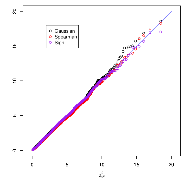
Rejection frequencies at $5\%$ nominal level are reported in Table 1 for the Gaussian, vdW, Spearman and sign tests based on the asymptotic critical values provided in Sections 5.1 and 6.1 but also for the vdW and Spearman tests based on bias-corrected critical values as described below. Inspection of Table 1 reveals that, under normal innovations, the rejection frequencies under the null hypothesis of the Gaussian test are very close to the nominal $5\%$ size. But the vdW and Spearman tests are quite below that nominal size, indicating a severe bias. This bias is confirmed by Figure 1, which shows the QQ plots of the values of the vdW test statistic across the $N=1000$ replications with Gaussian $f$ (but $f$ has no impact here, as the ranks are distribution-free under the null). The tails of the vdW statistic, for instance, very clearly do not match those of the chi-square they are converging to. The reason for this is the relatively slow convergence of the distribution of center-outward rank statistics: $n_{R}=20$ for $n=800$ is still a rather small $n_{R}$ value, which explains the phenomenon. Note that the same QQ plot for the sign test score statistic, which does not depend on the ranks, are more satisfactory.

Now, that bias of rank-based tests is easily corrected by considering permutational critical values instead of the asymptotic ones. The latter are obtained by generating $M$ permutations of the gridpoints ${\mathfrak{G}}^{(n)}$ , and taking the 0.95 quantile of the resulting $M$ values of the test statistic as a critical value instead of the chi-square quantile of order 0.95. The resulting tests have asymptotic size 5 % under the null. Their rejection frequencies are reported in Table 1 under the label “bias-corrected,” for the vdW and Spearman tests.

Refer to caption — Figure 1: QQ plots of the empirical distributions (across $N=1000$ replications) of the test statistics in Table 1 against their asymptotically chi-square null distributions: vdW (left), Gaussian, Spearman, and sign test scores (right).

Table 2: Numbers of under-, correct, and over-identification for the VAR(

1

) model under various innovation densities and additive outlier schemes, of the Gaussian, vdW, bias-corrected vdW, Spearman, bias-corrected Spearman, and sign tests out of

N=1000

replications; the sample size is

n=800

(

n_{R}=20

n_{S}=40

, and

n_{0}=0

); results of the sign tests with

n_{S}=n

are also included; permutational crirical values are based on

M=1000

random permutations.

		Order identification					Order identification
$\hskip 8.50012pt\ f$	Test	0	1	$\geq 2$	$\hskip 8.50012pt\ f$	Test	0	1	$\geq 2$
Normal					Mixture
	Gaussian	0	953	47		Gaussian	0	950	50
	vdW	0	990	10		vdW	0	991	9
	bias-corrected vdW	0	979	21		bias-corrected vdW	0	974	26
	Spearman	0	984	16		Spearman	0	980	20
	bias-corrected Spearman	0	982	18		bias-corrected Spearman	0	971	29
	Sign ( $n_{S}=40$ )	0	977	23		Sign ( $n_{S}=40$ )	0	972	28
	Sign ( $n_{S}=800$ )	0	979	21		Sign ( $n_{S}=800$ )	0	979	21
$t_{3}$					Skew- $t_{3}$
	Gaussian	0	908	92		Gaussian	0	855	145
	vdW	0	985	15		vdW	0	987	13
	bias-corrected vdW	0	961	39		bias-corrected vdW	0	970	30
	Spearman	0	973	27		Spearman	0	970	30
	bias-corrected Spearman	0	961	39		bias-corrected Spearman	0	968	32
	Sign ( ${}_{S}=40$ )	0	969	31		Sign ( $n_{S}=40$ )	0	981	19
	Sign ( $n_{S}=800$ )	0	968	32		Sign ( $n_{S}=800$ )	0	978	22
AOs ( ${\mbox{\boldmath$s$}}=(6,6)^{\prime}$ )					AOs ( ${\mbox{\boldmath$s$}}=(9,9)^{\prime}$ )
	Gaussian	0	933	67		Gaussian	0	878	122
	vdW	0	1000	0		vdW	0	1000	0
	bias-corrected vdW	0	1000	0		bias-corrected vdW	0	1000	0
	Spearman	0	1000	0		Spearman	0	1000	0
	bias-corrected Spearman	0	1000	0		bias-corrected Spearman	0	1000	0
	Sign ( $n_{S}=40$ )	0	998	2		Sign ( $n_{S}=40$ )	0	987	13
	Sign ( $n_{S}=800$ )	0	998	2		Sign ( $n_{S}=800$ )	0	990	10

The vdW and Spearman tests have greater power than the sign test and slightly less power than the Gaussian one under Gaussian innovations. Under $t_{3}$ innovations, however, the vdW and Spearman tests, despite their bias, both outperform the Gaussian test. The bias-corrected vdW and Spearman tests have correct size under the null and even higher powers; under the mixture and skew- $t_{3}$ innovations, they outperform the Gaussian test by a landslide. The tests based on signs have been implemented with the same factorization (viz., $n_{R}=20$ , $n_{S}=40$ , and $n_{0}=0$ ) as vdW and Spearman; the factorization ( $n_{R}=1$ , $n_{S}=800$ , and $n_{0}=\penalty\ \!0$ ) also has been considered, but provides little improvement. Turning to robustness issues, the resistance to additive outliers of the rank-based tests over the Gaussian one is extremely good, while the Gaussian test literally crashes, with exploding size under the null—the corresponding rejection frequencies under the alternative thus are meaningless. Despite their simplicity, the sign tests do extremely well (confirming univariate robustness results by Boldin, 2012; Boldin, 2013) but remain less powerful than the bias-corrected vdW tests. Bias-corrected tests uniformly outperform their uncorrected asymptotic counterparts.

7.2 VAR order identification

Turning to VAR order identification, let us consider the bivariate VAR(1) model with autoregression matrix coefficient $\text{vec}({\mbox{\boldmath$A$}})=(0.30,-0.06,0.12,0.24)^{\prime}$ , the same innovation densities and the same contamination schemes as in Section 7.1, and sample size $n=800$ . The sequential method of Sections 5.2 and 6.2 was applied to $N=1000$ replications thereof.

Each step consists in testing (at 5% nominal level) a VAR( $p$ ) against a VAR( $p+1$ ), which requires the estimation of the null VAR( $p$ ) model; throughout, this estimation is performed via the center-outward R-estimator based on vdW scores as proposed by Hallin et al., 2019, where it is shown to be root- $n$ consistent. The numbers of under-, correct, and over-identification for the Gaussian, (corrected) vdW, (corrected) Spearman, and (corrected) sign tests are reported in Table 2.

All tests are rejecting the hypothesis of white noise, irrespective of the underlying innovation density or the presence of outliers: no under-identifications, thus. Also, the rank-based procedures yield uniformly lower over-identification rates than the Gaussian one. Under the $t_{3}$ distribution, the Gaussian procedure yields an almost 10% over-identification rate, indicating that its performance is badly affected by heavy tails. The rank-based procedures, on the other hand, do much better under heavy tails, skewness, and additive outliers.

7.3 A real data example

To illustrate the applicability of our VAR order selection procedure, we consider the joint behaviour of two macroeconomic time series in the U.S. economy. Specifically, we downloaded the M1SL Money Stock and the Current Price Index All Urban Customers for All Items (labeled as M1SL and CPIAUCSL, respectively) time series from the Federal Reserve Bank of Saint Louis economic data server (see https://fred.stlouisfed.org). The M1SL includes funds that are readily accessible for spending and represent the most liquid portions of the money supply quickly convertible into cash. The CPIAUCSL is a measure of the average monthly change in the price for goods and services paid by urban consumers between any two time periods; we refer to U.S. Bureau of Labor Statistics for further technical details. In our statistical analysis, we consider monthly records for the period 01-Jan-1960 to 01-Sept-2020. For additional info, we refer to the Board of Governors of the Federal Reserve System. The joint semiparametric modeling of these series can be of help for monetary policy decisions.

Table 3: Values of test statistics and

p

-values (in parenthesis) of the Gaussian, vdW, Spearman, sign (

n_{S}=22

), and sign (

n_{S}=726

) tests, along with their

p

-values (in brackets) and (for vdW and Spearman) bias-corrected

p

-values (in square brackets) under the null hypotheses of a VAR(

p_{0}

) model (

p_{0}=0,...,7

$p_{0}$	Gaussian	vdW	Spearman	Sign ( $n_{S}=22$ )	Sign ( $n_{S}=726$ )
$0$	25.05 (4.91 $\times 10^{-5}$ )	224.67 (0) [0]	238.71 (0) [0]	356.90 (0)	342.58 (0)
$1$	25.83 (3.42 $\times 10^{-5}$ )	16.77 (0.002) [0.001]	15.42 (0.004) [0.001]	26.16 (2.94 $\times 10^{-5}$ )	59.14 (4.40 $\times 10^{-12}$ )
$2$	2.30 (0.681)	62.35 (9.30 $\times 10^{-13}$ ) [0]	71.57 (1.07 $\times 10^{-14}$ ) [0]	16.56 (0.002)	56.74 (1.40 $\times 10^{-11}$ )
$3$		48.59 (7.18 $\times 10^{-10}$ ) [0]	56.90 (1.30 $\times 10^{-11}$ ) [0]	47.99 (9.49 $\times 10^{-10}$ )	55.64 (2.38 $\times 10^{-11}$ )
$4$		10.74 (0.030) [0.016]	13.14 (0.011) [0.010]	26.58 (2.41 $\times 10^{-5}$ )	12.94 (0.012)
$5$		19.02 (7.81 $\times 10^{-5}$ ) [0]	21.37 (2.67 $\times 10^{-5}$ ) [0]	16.57 (0.002)	40.57 (3.29 $\times 10^{-8}$ )
$6$		7.58 (0.108) [0.068]	24.14 (7.49 $\times 10^{-5}$ ) [0.005]	32.58 (1.45 $\times 10^{-6}$ )	26.22 (2.85 $\times 10^{-5}$ )
$7$			4.27 (0.371) [0.322]	8.60 (0.072)	8.24 (0.083)

To start with, in the top panels of Figure 2, we display the seasonally adjusted time series. Even a visual inspection reveals some interesting characteristics. A first clearly visible aspect is that both time series display a trend in time. To deal with this, we differentiate the series and plot the resulting outputs in the bottom panels of Figure 2. We notice that the differentiated series seem to be correlated and display common movements (mainly in opposite directions). A second noticeable aspect is that, starting from 2005, the trajectories of the differentiated series look increasingly asymmetric and spiky. The period March-September-2020 reveals a cluster of outlying values, most likely due to COVID-19-related policy decisions.

A VAR model of appropriate order is likely to provide an adequately describe the joint behavior of the M1SL and CPIAUCSL series. However, the plots in Figure 2 suggest possible heavy tails and the presence, during the COVID-19 pandemic period, of large outliers. Gaussian procedures, therefore, might be inappropriate in view of the Monte Carlo analyses of Sections 7.1 and 7.2. To investigate that point, besides the traditional Gaussian one, we also ran, on the same series, the rank-based order-identification procedures described in Section 7.2. The results are shown in Table 3.

Inspection of Table 3 reveals a sharp contrast between the conclusions of the Gaussian and rank-nased methods. The Gaussian procedure indeed very clearly selects (at nominal level $5\%$ ) a VAR(2) model while all rank-based procedures, whether bias-corrected (with $M=1000$ permutations) or not, agree on a larger number of 6-7 lags.

Our educated guess is that the combination of skewness, kurtosis, and outliers are blurring the conclusions of Gaussian tests; the graphical diagnostics in Figure 3 bring some evidence in favor of that guess. Figure 3 displays the residuals of a VAR(7) fit of the M1SL and CPIAUCSL series. The panels show that the fitted residuals of each time series are centered about zero but asymmetrically scattered, apparently with heavy tails. The scatterplots (bottom panels) confirms the presence of skewness and kurtosis; some isolated, large outlying values are clearly visible, which supports our conjecture. These features of the underlying distribution obviously have a significant impact on the Gaussian procedure whereas our rank-based approach is much less affected.

8 Conclusion

This paper introduces rank-based tests for VAR models with unspecified innovation density. Based on the residual center-outward ranks and signs recently proposed by Chernozhukov et al., 2017 and (Hallin et al., 2020a, where they are shown to be essentially maximal ancillary), they constitute the testing counterpart of the R-estimators proposed in Hallin et al., 2019. When testing a VAR with specified parameter $\mbox{\boldmath$\theta$}_{0}$ , they are fully distribution-free; when $\mbox{\boldmath$\theta$}_{0}$ remains unspecified under the null, they are strongly asymptotically distribution-free in the sense of being asymptotically equal to a fully-distribution-free test. When based on appropriate score functions, they achieve parametric efficiency at selected reference densities. Monte Carlo experiments and an empirical example demonstrate the excellent performance of the proposed tests, which significantly outperform the traditional pseudo-Gaussian methods under skew, heavy-tailed, and contaminated innovations.

References

Azzalini and Capitanio, (2003) Azzalini, A. and Capitanio, A. (2003). Distributions generated by perturbation of symmetry with emphasis on a multivariate skew t-distribution. J. R. Statist. Soc. B, 65, 367–389.
del Barrio et al., (2020) del Barrio, E., González-Sanz, A., and Hallin, M. (2020). A note on the regularity of optimal-transport-based center-outward distribution and quantile functions. J. Multivariate Anal., in press.
Benghabrit and Hallin, (1992) Benghabrit, Y. and Hallin, M. (1992). Optimal rank-based tests against first-order superdiagonal bilinear dependence. J. Statist. Plann. Inference, 32, 45–61.
Benghabrit and Hallin, (1996) Benghabrit, Y. and Hallin, M. (1996). Rank-based tests for autoregressive against bilinear dependence. J. Nonparametric Stat., 6, 253–272.
Bertsekas, (1991) Bertsekas, D., (1991). Linear Network Optimization. Algorithms and Codes. MIT Press, Cambridge, MA.
Boldin, (2012) Boldin M.V. (2012). Robustness of sign tests in autoregression. Moscow Math. Bull., 67, 112–115.
Boldin, (2013) Boldin M.V. (2013). Robustness of sign tests for testing hypotheses about the order of autoregression. Theory Probab. Appl., 57, 663–670.
Brockwell and Davis, (1987) Brockwell, P. J. and Davis, R. A. (1987). Time Series: Theory and Methods. Springer, N.Y.
Burkhard et al., (2009) Burkhard, R., Dell’Amico, M., and Martello, S. (2009). Assignment Problems, SIAM.
Cassart et al, (2010) Cassart, D., Hallin, M., and Paindaveine, D. (2010). On the estimation of cross-information quantities in R-estimation. In J. Antoch, M. Hušková, and P.K. Sen, Eds: Nonparametrics and Robustness in Modern Statistical Inference and Time Series Analysis: A Festschrift in Honor of Professor Jana Jurečková, I.M.S., 35–45.
Chernozhukov et al., (2017) Chernozhukov, V., Galichon, A., Hallin, M., and Henry, M. (2017). Monge-Kantorovich depth, quantiles, ranks, and signs, Ann. Statist., 45, 223–256.
Croux, (2008) Croux, C. and Joossens, K. (2008). Robust estimation of the vector autoregressive model by a least trimmed squares procedure. COMPSTAT 2008, 489-501.
Deb and Sen, (2019) Deb, N. and Sen, B. (2019). Multivariate rank-based distribution-free nonparametric testing using measure transportation, arXiv:1909.08733.
Dick and Pillichshammer, (2014) Dick, J. and Pillichshammer, F. (2014). Discrepancy theory and quasi-Monte Carlo integration, in W. Chen, A. Sirvastava and G. Travaglini, Eds, A Panorama of Discrepancy Theory, 539-620, Springer, N.Y.
Durbin and Watson, (1950) Durbin, J. and Watson, G.S. (1950). Testing for serial correlation in least squares regression I. Biometrika, 37, 409–428.
Durbin and Watson, (1951) Durbin, J. and Watson, G.S. (1951). Testing for serial correlation in least squares regression II. Biometrika, 38, 159–179.
Figalli, (2018) Figalli, A. (2018). On the continuity of center-outward distribution and quantile functions, Nonlinear Anal., 177, part B, 413-421.
Garel and Hallin, (1995) Garel, B. and Hallin, M. (1995). Local asymptotic normality of multivariate ARMA processes with a linear trend. Ann. Inst. Statist. Math., 3, 551-579.
Garel and Hallin, (1999) Garel, B. and Hallin, M. (1999). Rank-based autoregressive order identification. J. Amer. Statist. Assoc., 94, 1357-1371.
Ghosal and Sen, (2019) Ghosal, P. and Sen, B. (2019). Multivariate ranks and quantiles using optimal transportation and applications to goodness-of-fit testing, arXiv:1905.05340.
Hájek, (1961) Hájek, J.. (1961). Some extensions of the Wald-Wolfowitz-Noether theorem, Ann. Math. Statist., 32, 506–523.
Hájek and Šidák, (1967) Hájek, J., and Šidák, Z. (1967). Theory of Rank Tests. Academic Press, N.Y.
Hallin, (1986) Hallin, M. (1986). Non-stationary $q$ -dependent processes and time-varying moving-average models: invertibility properties and the forecasting problem. Adv. in Appl. Probab., 18, 170-210.
Hallin, (1994) Hallin, M. (1994). On the Pitman nonadmissibility of correlogram-based time series methods, J. Time Series Anal. 16, 607–612.
Hallin, (2017) Hallin, M. (2017). On distribution and quantile functions, ranks and signs in $\mathbb{R}^{d}$ . ECARES WP. Available at https://ideas.repec.org/p/eca/wpaper/2013-258262.html.
(26) Hallin, M., del Barrio, E., Cuesta-Albertos, J., and Matrán, C. (2020a). Center-outward distribution and quantile functions, ranks, and signs in dimension $d$ : a measure transportation approach, Ann. Statist., in press.
(27) Hallin, M., Hlubinka, D., and Hudecová, Š. (2020b). Fully distribution-free center-outward rank tests for multiple-output regression and MANOVA, arXiv:2007.15496.
Hallin et al., (1985) Hallin, M., Ingenbleek, J.-Fr., and Puri, M.L. (1985). Linear serial rank tests for randomness against ARMA alternatives, Ann. Statist., 13, 1156–1181.
Hallin and La Vecchia, (2017) Hallin, M. and La Vecchia, D. (2017). R-estimation in semiparametric dynamic location-scale models. J. Econometrics, 196, 233–247.
Hallin and La Vecchia, (2020) Hallin, M. and La Vecchia, D. (2020). A simple R-estimation method for semiparametric duration models. J. Econometrics, 218, 736–749.
Hallin et al., (2019) Hallin, M., La Vecchia, D. and Liu, H. (2019). Center-outward R-estimation for semiparametric VARMA models. J. Amer. Statist. Assoc., in press; arXiv:1910.08442.
Hallin and Mélard, (1988) Hallin, M. and Mélard, G. (2002a). Rank-based tests for randomness against first-order serial dependence. J. Amer. Statist. Assoc., 83, 1117–1129.
Hallin et al, (2006) Hallin, M., Oja, H., and Paindaveine, D. (2006). Semiparametrically efficient rank-based inference for shape: II Optimal R-estimation of shape, Ann. Statist., 34, 2757–2789.
Hallin and Paindaveine, (2002) Hallin, M. and Paindaveine, D. (2002a). Optimal tests for multivariate location based on interdirections and pseudo-Mahalanobis ranks. Ann. Statist., 30, 1103–1133.
(35) Hallin, M. and Paindaveine, D. (2004a). Rank-based optimal tests of the adequacy of an elliptic VARMA model. Ann. Statist., 6, 2642–2678.
(36) Hallin, M. and Paindaveine, D. (2004b). Multivariate signed-rank tests in vector autoregressive order identification. Statist. Sci., 4, 697–711.
Hallin and Paindaveine, (2005) Hallin, M. and Paindaveine, D. (2005). Affine-invariant aligned rank tests for the multivariate general linear model with VARMA errors. J. Multivariate Anal., 1, 122-163.
Hallin and Paindaveine, (2006) Hallin, M. and Paindaveine, D. (2006a). Semiparametrically efficient rank-based inference for shape: I Optimal rank-based tests for sphericity, Ann. Statist. 34, 2707–2756.
Hallin and Paindaveine, (2008) Hallin, M. and Paindaveine, D. (2008b). Optimal rank-based tests for homogeneity of scatter, Ann. Statist., 36, 1261-1298.
Hallin et al., (2010) Hallin, M., Paindaveine, D., and Verdebout, T. (2010). Optimal rank-based testing for principal components. Ann. Statist., 38, 3245–3299.
Hallin et al., (2013) Hallin, M., Paindaveine, D., and Verdebout, T. (2013). Optimal rank-based tests for common principal components. Bernoulli, 19, 2524–2556.
Hallin et al., (2014) Hallin, M., Paindaveine, D., and Verdebout, T. (2014). Efficient R-estimation of principal and common principal components, J. Amer. Statist. Assoc., 109, 1071–1083.
Hallin and Puri, (1988) Hallin, M. and Puri, M.L. (1988). Optimal rank-based procedures for time-series analysis: testing an ARMA model against other ARMA models. Ann. Statist., 16, 402–432.
Hallin and Puri, (1991) Hallin, M. and Puri, M.L. (1981). Time-series analysis via rank-order theory: signed-rank tests for ARMA models, J. Multivar. Anal. 39, 1–29.
Hallin and Puri, (1994) Hallin, M. and Puri, M.L. (1994). Aligned rank tests for linear models with autocorrelated error terms, J. Multivar. Anal., 50, 175–237.
Hallin and Vermandele, (1996) Hallin, M. and Vermandele, C. (1996). A simple proof of asymptotic normality for simple serial rank statistics. In E. Brunner and M. Denker, Eds., Research Developments in Probability and Statistics, Festschrift in Honor of Madan L. Puri, VSP, Utrecht, the Netherlands, 163–191.
Hallin and Werker, (2003) Hallin, M. and Werker, B.J.M. (2003). Semiparametric efficiency, distribution-freeness, and invariance, Bernoulli 9, 137–165.
Judd, (1998) Judd, K.L. (1998). Num. Meth. Econ., MIT Press, Cambridge, MA.
Kreiss, (1987) Kreiss, J.-P. (1987). On adaptative estimation in stationary ARMA processes, Ann. Statist., 15, 112–133.
Le Cam, (1986) Le Cam, L. (1986). Asymptotic Methods in Statistical Decision Theory, Springer, N.Y.
Le Cam and Yang, (2000) Le Cam, L. and Yang, G. L. (2000). Asymptotics in Statistics : Some basic concepts (2nd edition). Springer, N.Y.
Lehmann and Romano, (2005) Lehmann, E.L. and Romano, J.P. (2005). Testing Statistical Hypotheses, Springer, N.Y.
Mancini et al., (2005) Macini, L., Ronchetti, E., Trojani, F. (2005), Optimal conditionally unbiased bounded-influence inference in dynamics location and scale models, J. Amer. Statist. Assoc., 100, 628-641.
Mérigot, (2005) Mérigot, Q. (2011). A multiscale approach to optimal transport, Comp. Graph. Forum, 30, 1583-1592.
Niederreiter, (1992) Niederreiter, H. (1992). Random Number Generation and Quasi-Monte Carlo Methods. CBMS-NSF Regional Conference Series in Applied Mathematics, 63, SIAM, Philadelphia, PA.
Peyré and Cuturi, (2019) Peyré, G. and Cuturi, M. (2019). Computational optimal transport with applications to Data Science. Found. Trends Machine Learn., 11, 355–607.
Pötscher, (1983) Pötscher, B.M. (1983). Order estimation in ARMA models by Lagrangian multiplier tests, Ann. Statist., 11, 872-885.
Shi et al., (2019) Shi, H., Drton, M., and Han, F. (2019). Distribution-free consistent independence tests via Hallin’s multivariate ranks, arXiv:1909.10024.
Shi et al., (2020) Shi, H., Hallin, M., Drton, M., and Han, F. (2020). Rate-optimality of consistent distribution-free tests of independence based on center-outward ranks and signs, arXiv:2007.02186.
Shorack, (2000) Shorack, G.R. (2000). Probability for Statisticians. Springer, N.Y.
van der Vaart, (1998) van der Vaart, A. (1998). Asymptotic Statistics. Cambridge University Press, Cambridge.

Appendix A: Algebraic preparation for LAN

Some linear difference equation algebra is required in order to obtain the explicit form of the central sequences and information matrices in the LAN result of Section 2.2—to be used in the construction of our center-outward rank-based test statistics.

Denote by ${\mbox{\boldmath$G$}}_{u}$ , $u\in{\mathbb{Z}}$ the Green’s matrices associated with the difference operator ${\mbox{\boldmath$A$}}_{\mbox{\boldmath$\theta$}_{0}}(L)$ , with $\mbox{\boldmath$\theta$}_{0}\in{\mbox{\boldmath$\Theta$}}_{0}\subset{\mbox{\boldmath$\Theta$}}_{1}\subset\mathbb{R}^{p_{1}d^{2}}$ for some $p_{0}<p_{1}$ ; those matrices are defined as the solutions of the homogeneous linear recursions

{\mbox{\boldmath$A$}}_{\mbox{\boldmath$\theta$}_{0}}(L){\mbox{\boldmath$G$}}_{u}={\mbox{\boldmath$G$}}_{u}-\sum_{i=1}^{p_{0}}{\mbox{\boldmath$A$}}_{i}{\mbox{\boldmath$G$}}_{u-i}={\bf 0},\quad u\in\mathbb{Z}

with initial values ${\mbox{\boldmath$I$}}_{d},{\bf 0},\ldots,{\bf 0}$ at $u=0,-1,\ldots,-p_{0}+1$ .

For $\mbox{\boldmath$\theta$}_{0}\in{\mbox{\boldmath$\Theta$}}$ , the decrease of $\{\|{\mbox{\boldmath$G$}}_{u}\|,u\in{\mathbb{N}}\}$ as $u\to\infty$ is exponential. Specifically, there exists some $\varepsilon>0$ (depending on the smallest root of the equation $\text{\rm det}\left({\mbox{\boldmath$A$}}_{\mbox{\boldmath$\theta$}}(z)\right)\penalty\ \!=\penalty\ \!0$ ) such that $\|{\mbox{\boldmath$G$}}_{u}\|(1+\varepsilon)^{u}$ converges to $0$ as $u\rightarrow\infty$ . Denoting by ${\mbox{\boldmath$X$}}_{-p_{0}+1},\ldots,{\mbox{\boldmath$X$}}_{0}$ the initial values (which are typically unobservable) of a solution of the homogenous difference equation ${\mbox{\boldmath$A$}}_{\mbox{\boldmath$\theta$}_{0}}(L){\mbox{\boldmath$X$}}_{t}={\bf 0}$ , this exponential decrease ensures that these initial values have no asymptotic influence on asymptotic results and, therefore, safely can be set to zero in the sequel. This allows us to invert the autoregressive polynomial; the Green matrices ${\mbox{\boldmath$G$}}_{u}$ then are the matrix coefficients¹²¹² 12 In the econometric terminology, the impulse response matrix coefficients. of the inverted operator ${\mbox{\boldmath$A$}}_{\mbox{\boldmath$\theta$}_{0}}(L)^{-1}$ :

{\mbox{\boldmath$A$}}_{\mbox{\boldmath$\theta$}_{0}}(z)^{-1}=\sum_{u=0}^{\infty}{\mbox{\boldmath$G$}}_{u}z^{u}:=\left({\mbox{\boldmath$I$}}_{d}-\sum_{i=1}^{p_{0}}{\mbox{\boldmath$A$}}_{i}z^{i}\right)^{-1},\quad z\in{\mbox{\boldmath$C$}},|z|<1.

More generally, associated with an arbitrary $d$ -dimensional linear difference ope-rator ${\mbox{\boldmath$C$}}(L):=\sum_{i=0}^{\infty}{\mbox{\boldmath$C$}}_{i}L^{i}$ (this of course includes operators of finite order $s$ ), define, for any integers $v\leq u$ , the $d^{2}u\times d^{2}v$ matrices (the form of which is motivated by the vec ${\mbox{\boldmath$A$}}_{u}$ form under which the VAR matrix coefficients ${\mbox{\boldmath$A$}}_{u}$ enter $\mbox{\boldmath$\theta$}_{0}$ and the $d^{2}v$ -dimension nature of the perturbations $\tau$ on the LAN property )

{\mbox{\boldmath$C$}}_{u,v}:=\begin{bmatrix}{\mbox{\boldmath$C$}}_{0}\otimes{\mbox{\boldmath$I$}}_{d}&{\mbox{\boldmath$0$}}&\ldots&{\mbox{\boldmath$0$}}\\ {\mbox{\boldmath$C$}}_{1}\otimes{\mbox{\boldmath$I$}}_{d}&{\mbox{\boldmath$C$}}_{0}\otimes{\mbox{\boldmath$I$}}_{d}&\ldots&{\mbox{\boldmath$0$}}\\ \vdots&&\ddots&\vdots\\ {\mbox{\boldmath$C$}}_{v-1}\otimes{\mbox{\boldmath$I$}}_{d}&{\mbox{\boldmath$C$}}_{v-2}\otimes{\mbox{\boldmath$I$}}_{d}&\ldots&{\mbox{\boldmath$C$}}_{0}\otimes{\mbox{\boldmath$I$}}_{d}\\ \vdots&&&\vdots\\ {\mbox{\boldmath$C$}}_{u-1}\otimes{\mbox{\boldmath$I$}}_{d}&{\mbox{\boldmath$C$}}_{u-2}\otimes{\mbox{\boldmath$I$}}_{d}&\ldots&{\mbox{\boldmath$C$}}_{u-v}\otimes{\mbox{\boldmath$I$}}_{d}\end{bmatrix}.

With this notation, ${\mbox{\boldmath$G$}}_{u,u}$ (associated with ${\mbox{\boldmath$C$}}(L)={\mbox{\boldmath$A$}}_{\mbox{\boldmath$\theta$}_{0}}(L)^{-1}$ ) is the inverse of ${\mbox{\boldmath$A$}}_{u,u}$ (associated with ${\mbox{\boldmath$C$}}(L)={\mbox{\boldmath$A$}}_{\mbox{\boldmath$\theta$}_{0}}(L)$ ). Denoting by ${\mbox{\boldmath$C$}}_{u,v}^{\prime}$ the matrices associated with the transposed operator ${\mbox{\boldmath$C$}}^{\prime}(L):=\sum_{i=0}^{\infty}{\mbox{\boldmath$C$}}^{\prime}_{i}L^{i}$ , we also have that ${\mbox{\boldmath$G$}}_{u,u}^{\prime}=({\mbox{\boldmath$A$}}_{u,u}^{\prime})^{-1}$ . Then, for any $\mbox{\boldmath$\theta$}_{0}\in{\mbox{\boldmath$\Theta$}}_{0}$ and any $p_{1}>p_{0}$ , the $d^{2}p_{1}\times d^{2}p_{1}$ matrix

{\mbox{\boldmath$M$}}_{\mbox{\boldmath$\theta$}_{0}}:={\mbox{\boldmath$G$}}^{\prime}_{p_{1},p_{1}};

(A.1)

is of full rank.

Still associated with ${\mbox{\boldmath$A$}}_{\mbox{\boldmath$\theta$}_{0}}(L)$ , consider the operator ${\mbox{\boldmath$D$}}_{\mbox{\boldmath$\theta$}_{0}}(L):={\mbox{\boldmath$I$}}_{d}+\sum_{i=1}^{p_{0}}{\mbox{\boldmath$D$}}_{i}L^{i}$ where

\begin{bmatrix}{\mbox{\boldmath$D$}}_{1}^{\prime}\\ \vdots\\ {\mbox{\boldmath$D$}}_{p_{0}}^{\prime}\end{bmatrix}:=-\begin{bmatrix}{\mbox{\boldmath$G$}}_{0}&{\mbox{\boldmath$G$}}_{-1}&\ldots&{\mbox{\boldmath$G$}}_{-p_{0}+1}\\ {\mbox{\boldmath$G$}}_{1}&{\mbox{\boldmath$G$}}_{0}&\ldots&{\mbox{\boldmath$G$}}_{-p_{0}+2}\\ \vdots&&\ddots&\vdots\\ {\mbox{\boldmath$G$}}_{p_{0}-1}&{\mbox{\boldmath$G$}}_{p_{0}-2}&\ldots&{\mbox{\boldmath$G$}}_{0}\\ \end{bmatrix}^{-1}\begin{bmatrix}{\mbox{\boldmath$G$}}_{1}\\ \vdots\\ {\mbox{\boldmath$G$}}_{p_{0}}\end{bmatrix}

(recall that ${\mbox{\boldmath$G$}}_{-1}={\mbox{\boldmath$G$}}_{-2}=\cdots={\mbox{\boldmath$G$}}_{-p_{0}+1}={\mbox{\boldmath$0$}}$ ).

Let $\{\mbox{\boldmath$\psi$}_{t}^{(1)},\ldots,\mbox{\boldmath$\psi$}_{t}^{(p_{0})}\}$ be any set of $d\times d$ matrices forming a fundamental system of solutions of the homogeneous linear difference equation associated with ${\mbox{\boldmath$D$}}_{\mbox{\boldmath$\theta$}_{0}}(L)$ . Such a system can be obtained, for instance, from the Green matrices of ${\mbox{\boldmath$D$}}_{\mbox{\boldmath$\theta$}_{0}}(L)$ (see, e.g., Hallin, 1986). Defining

{\boldsymbol{\Psi}}_{m}(\mbox{\boldmath$\theta$}_{0}):=\begin{bmatrix}\mbox{\boldmath$\psi$}_{p_{1}-p_{0}+1}^{(1)}&\ldots&\mbox{\boldmath$\psi$}_{p_{1}-p_{0}+1}^{(p_{0})}\\ \mbox{\boldmath$\psi$}_{p_{1}-p_{0}+2}^{(1)}&\ldots&\mbox{\boldmath$\psi$}_{p_{1}-p_{0}+2}^{(p_{0})}\\ \vdots&&\vdots\\ \mbox{\boldmath$\psi$}_{m}^{(1)}&\ldots&\mbox{\boldmath$\psi$}_{m}^{(p_{0})}\end{bmatrix}\otimes{\mbox{\boldmath$I$}}_{d}\qquad(m>p_{1}-p_{0}),

the Casorati matrix associated with ${\mbox{\boldmath$D$}}_{\mbox{\boldmath$\theta$}_{0}}(L)$ is ${\boldsymbol{\Psi}}_{p_{1}}$ , which has full rank. Finally, let

{\mbox{\boldmath$P$}}_{\mbox{\boldmath$\theta$}_{0}}:=\begin{bmatrix}{\mbox{\boldmath$I$}}_{d^{2}(p_{1}-p_{0})}&{\mbox{\boldmath$0$}}\\ {\mbox{\boldmath$0$}}&{\boldsymbol{\Psi}}_{p_{1}}^{-1}(\mbox{\boldmath$\theta$}_{0})\end{bmatrix}\quad\text{and}\quad{\mbox{\boldmath$Q$}}^{(n)}_{\mbox{\boldmath$\theta$}_{0}}:=\begin{bmatrix}{\mbox{\boldmath$I$}}_{d^{2}(p_{1}-p_{0})}&{\mbox{\boldmath$0$}}\\ {\mbox{\boldmath$0$}}&{\boldsymbol{\Psi}}_{n-1}(\mbox{\boldmath$\theta$}_{0})\end{bmatrix}.

(A.2)

Note that while ${\mbox{\boldmath$M$}}_{\mbox{\boldmath$\theta$}_{0}}$ , ${\mbox{\boldmath$P$}}_{\mbox{\boldmath$\theta$}_{0}}$ , and ${\mbox{\boldmath$Q$}}_{\mbox{\boldmath$\theta$}_{0}}^{(n)}$ depend on the choice of the fundamental system $\{\mbox{\boldmath$\psi$}_{t}^{(1)},\ldots,\mbox{\boldmath$\psi$}_{t}^{(p_{0})}\}$ , the product ${\mbox{\boldmath$M$}}_{\mbox{\boldmath$\theta$}_{0}}^{\prime}{\mbox{\boldmath$P$}}_{\mbox{\boldmath$\theta$}_{0}}^{\prime}{\mbox{\boldmath$Q$}}_{\mbox{\boldmath$\theta$}_{0}}^{(n)\prime}$ appearing in the definition of the central sequence (2.4) does not. We refer to Hallin and Paindaveine, 2004a for details.

Appendix B: Proofs of Proposition 3.1 and Lemma 3.1

Let ${\mbox{\boldmath$a$}}_{t,s}^{(n)}:={\mbox{\boldmath$a$}}({\mbox{\boldmath$F$}}^{(n)}_{\pm,t},{\mbox{\boldmath$F$}}^{(n)}_{\pm,s})$ . The following Lemmas will be used to prove Proposition 3.1; throughout this section, ${\rm E}$ stands for ${\rm E}_{\mbox{\boldmath$\theta$}_{0};f}$ ( $f\in{\cal F}_{d}$ ).

Lemma B1.

${\rm E}({\mbox{\boldmath$a$}}_{2,1}^{(n)})=\frac{(n-2)(n-3)}{n(n-1)}{\rm E}({\mbox{\boldmath$a$}}_{2,1}^{(n)}|{\mbox{\boldmath$F$}}^{(n)}_{\pm,4},{\mbox{\boldmath$F$}}^{(n)}_{\pm,3})+\frac{1}{n(n-1)}{\mbox{\boldmath$b$}}^{(n)}_{4,3}$ , where

	$\displaystyle{\mbox{\boldmath$b$}}^{(n)}_{4,3}:=$	$\displaystyle(n-2)\Big[{\rm E}({\mbox{\boldmath$a$}}_{4,1}^{(n)}\|{\mbox{\boldmath$F$}}^{(n)}_{\pm,4},{\mbox{\boldmath$F$}}^{(n)}_{\pm,3})+{\rm E}({\mbox{\boldmath$a$}}_{3,1}^{(n)}\|{\mbox{\boldmath$F$}}^{(n)}_{\pm,4},{\mbox{\boldmath$F$}}^{(n)}_{\pm,3})+{\rm E}({\mbox{\boldmath$a$}}_{2,4}^{(n)}\|{\mbox{\boldmath$F$}}^{(n)}_{\pm,4},{\mbox{\boldmath$F$}}^{(n)}_{\pm,3})$
		$\displaystyle+{\rm E}({\mbox{\boldmath$a$}}_{2,3}^{(n)}\|{\mbox{\boldmath$F$}}^{(n)}_{\pm,4},{\mbox{\boldmath$F$}}^{(n)}_{\pm,3})\Big]+{\rm E}({\mbox{\boldmath$a$}}_{3,4}^{(n)}\|{\mbox{\boldmath$F$}}^{(n)}_{\pm,4},{\mbox{\boldmath$F$}}^{(n)}_{\pm,3})+{\rm E}({\mbox{\boldmath$a$}}_{4,3}^{(n)}\|{\mbox{\boldmath$F$}}^{(n)}_{\pm,4},{\mbox{\boldmath$F$}}^{(n)}_{\pm,3}).$

Proof.

The proof follows from an enumeration of the $n(n-1)$ terms in $\underset{1\leq i_{1}\neq i_{2}\leq n}{\sum\sum}{\mbox{\boldmath$a$}}_{i_{1},i_{2}}^{(n)}\vskip 2.84526pt$ , which contains $(n-2)(n-3)$ terms with indices $i_{1}\neq i_{2}$ such that $\#[\{i_{1}\neq i_{2}\}\cap\{3,4\}]=0$ , $4(n-2)$ terms with indices $i_{1}\neq i_{2}$ such that $\#[\{i_{1}\neq i_{2}\}\cap\{3,4\}]=1$ and $2$ terms with indices $i_{1}\neq i_{2}$ such that $\#[\{i_{1}\neq i_{2}\}\cap\{3,4\}]=2$ . ∎

Lemma B2.

$\left|{\rm E}({\mbox{\boldmath$a$}}_{2,1}^{(n)\prime}{\mbox{\boldmath$a$}}_{4,3}^{(n)})\right|\leq\frac{n(n-1)}{(n-2)(n-3)}{\rm E}({\mbox{\boldmath$a$}}_{2,1}^{(n)\prime}){\rm E}({\mbox{\boldmath$a$}}_{2,1}^{(n)})+\frac{4(n-2)+2}{(n-2)(n-3)}{\rm E}\left\|{\mbox{\boldmath$a$}}_{2,1}^{(n)}\right\|^{2}.$

Proof.

Lemma B1 implies

	$\displaystyle\left\|{\rm E}({\mbox{\boldmath$a$}}_{2,1}^{(n)\prime}{\mbox{\boldmath$a$}}_{4,3}^{(n)})\right\|$	$\displaystyle=\left\|{\rm E}\left[{\rm E}\left({\mbox{\boldmath$a$}}_{2,1}^{(n)\prime}\big\|{\mbox{\boldmath$F$}}^{(n)}_{\pm,4},{\mbox{\boldmath$F$}}^{(n)}_{\pm,3}\right){\mbox{\boldmath$a$}}_{4,3}^{(n)}\right]\right\|$
		$\displaystyle\leq\frac{n(n-1)}{(n-2)(n-3)}{\rm E}({\mbox{\boldmath$a$}}_{2,1}^{(n)\prime}){\rm E}({\mbox{\boldmath$a$}}_{4,3}^{(n)})+\frac{1}{(n-2)(n-3)}\left\|{\rm E}({\mbox{\boldmath$b$}}^{(n)\prime}_{4,3}{\mbox{\boldmath$a$}}_{4,3}^{(n)})\right\|$
		$\displaystyle=:\frac{n(n-1)}{(n-2)(n-3)}C^{(n)}_{1}+\frac{1}{(n-2)(n-3)}C^{(n)}_{2},\quad\text{say.}$

The desired result then follows from the fact that $C^{(n)}_{1}={\rm E}({\mbox{\boldmath$a$}}_{2,1}^{(n)})={\rm E}({\mbox{\boldmath$a$}}_{4,3}^{(n)})$ and the inequality $C^{(n)}_{2}\leq(4(n-2)+2){\rm E}\left\|{\mbox{\boldmath$a$}}_{2,1}^{(n)}\right\|^{2}$ . More specifically, note that

	$\displaystyle\left\|{\rm E}({\mbox{\boldmath$b$}}^{(n)\prime}_{4,3}{\mbox{\boldmath$a$}}_{4,3}^{(n)})\right\|$	$\displaystyle\leq(n-2)\Big(\left\|{\rm E}({\mbox{\boldmath$a$}}_{4,1}^{(n)\prime}{\mbox{\boldmath$a$}}_{4,3}^{(n)})\right\|+\left\|{\rm E}({\mbox{\boldmath$a$}}_{3,1}^{(n)\prime}{\mbox{\boldmath$a$}}_{4,3}^{(n)})\right\|+\left\|{\rm E}({\mbox{\boldmath$a$}}_{2,4}^{(n)\prime}{\mbox{\boldmath$a$}}_{4,3}^{(n)})\right\|+\left\|{\rm E}({\mbox{\boldmath$a$}}_{2,3}^{(n)\prime}{\mbox{\boldmath$a$}}_{4,3}^{(n)})\right\|\Big)$
		$\displaystyle\quad+\left\|{\rm E}({\mbox{\boldmath$a$}}_{3,4}^{(n)\prime}{\mbox{\boldmath$a$}}_{4,3}^{(n)})\right\|+\left\|{\rm E}({\mbox{\boldmath$a$}}_{4,3}^{(n)\prime}{\mbox{\boldmath$a$}}_{4,3}^{(n)})\right\|$
		$\displaystyle=:(n-2)\Big(C^{(n)}_{21}+C^{(n)}_{22}+C^{(n)}_{23}+C^{(n)}_{24}\Big)+C^{(n)}_{25}+C^{(n)}_{26},\quad\text{say.\vskip-5.69054pt}$

It follows from

\left|{\rm E}({\mbox{\boldmath$a$}}_{4,1}^{(n)\prime}{\mbox{\boldmath$a$}}_{4,3}^{(n)})\right|\leq({\rm E}\|({\mbox{\boldmath$a$}}_{4,1}^{(n)}\|^{2})^{1/2}({\rm E}\|({\mbox{\boldmath$a$}}_{4,3}^{(n)}\|^{2})^{1/2}={\rm E}\left\|{\mbox{\boldmath$a$}}_{2,1}^{(n)}\right\|^{2}

that $C^{(n)}_{21}\leq{\rm E}\left\|{\mbox{\boldmath$a$}}_{2,1}^{(n)}\right\|^{2}$ . For the same reason, we have $C^{(n)}_{2j}\leq{\rm E}\left\|{\mbox{\boldmath$a$}}_{2,1}^{(n)}\right\|^{2},\ j=2,...,6$ . The result then follows. ∎

Proof of Proposition 3.1. Due to LAN, it is sufficient to prove the desired result under ${\rm P}^{(n)}_{\mbox{\boldmath$\theta$}_{0};f}$ ( $f\in{\cal F}_{d}$ ). Let ${\mbox{\boldmath$\alpha$}}_{t,s}^{(n)}\!:=\!(\mbox{\boldmath$\xi$}_{t,s}^{(n)}-{\mbox{\boldmath$\gamma$}}^{(n)})-(\mbox{\boldmath$\xi$}_{t,s}-{\mbox{\boldmath$\gamma$}}),$ where

\mbox{\boldmath$\xi$}_{t,s}^{(n)}\!:=\!\text{vec}({\mbox{\boldmath$a$}}({\mbox{\boldmath$F$}}^{(n)}_{\pm,t},{\mbox{\boldmath$F$}}^{(n)}_{\pm,s})),\ \ \mbox{\boldmath$\xi$}_{t,s}\!:=\!\text{vec}({\mbox{\boldmath$J$}}_{1}({\mbox{\boldmath$F$}}_{\pm,t}){\mbox{\boldmath$J$}}_{2}^{\prime}({\mbox{\boldmath$F$}}_{\pm,s})),\ \ {\mbox{\boldmath$\gamma$}}^{(n)}\!\!:=\!\text{vec}({\mbox{\boldmath$m$}}^{(n)}),\text{ and }{\mbox{\boldmath$\gamma$}}\!:=\!\text{vec}({\mbox{\boldmath$m$}}).

We have

		$\displaystyle{\rm E}\left\\|(n-i)^{1/2}\text{\rm vec}(\hbox{\hskip 3.45831pt\hskip-3.45831pt\hbox{$\mbox{\boldmath$\Gamma$}$}\hskip-3.45831pt\hskip-4.09721pt\raisebox{-2.98203pt}{\hbox{$\scriptscriptstyle\thicksim$}}\hskip-4.09721pt\hskip 3.45831pt}_{i,{\mbox{\boldmath$J$}}_{1},{\mbox{\boldmath$J$}}_{2}}^{(n)}(\mbox{\boldmath$\theta$}_{0})-{\mbox{\boldmath$m$}}^{(n)}-\underline{\mbox{\boldmath$\Gamma$}}_{i,{\mbox{\boldmath$J$}}_{1},{\mbox{\boldmath$J$}}_{2}}^{(n)}(\mbox{\boldmath$\theta$}_{0})+{\mbox{\boldmath$m$}})\right\\|^{2}={\rm E}\Big\\|(n-i)^{-1/2}\sum_{t=i+1}^{n}{\mbox{\boldmath$\alpha$}}_{t,t-i}^{(n)}\Big\\|^{2}$
		$\displaystyle=(n-i)^{-1}\!\!\sum_{t=i+1}^{n}\!{\rm E}\\|{\mbox{\boldmath$\alpha$}}_{t,t-i}^{(n)}\\|^{2}\!+2(n-i)^{-1}\!\!\underset{\begin{subarray}{c}i+1\leq t,s\leq n\\ t=s-i\end{subarray}}{\sum\sum}\!{\rm E}({\mbox{\boldmath$\alpha$}}_{t,t-i}^{(n)\prime}{\mbox{\boldmath$\alpha$}}_{s,s-i}^{(n)})+(n-i)^{-1}\!\!\underset{\begin{subarray}{c}i+1\leq t,s\leq n\\ t\neq s,s-i\\ s\neq t-i\end{subarray}}{\sum\sum}\!{\rm E}({\mbox{\boldmath$\alpha$}}_{t,t-i}^{(n)\prime}{\mbox{\boldmath$\alpha$}}_{s,s-i}^{(n)})$
		$\displaystyle={\rm E}\\|{\mbox{\boldmath$\alpha$}}_{2,1}^{(n)}\\|^{2}+\frac{2(n-2i)}{n-i}{\rm E}({\mbox{\boldmath$\alpha$}}_{2,1}^{(n)\prime}{\mbox{\boldmath$\alpha$}}_{3,2}^{(n)})+\frac{(n-i)^{2}-(n-i)-2(n-2i)}{n-i}{\rm E}({\mbox{\boldmath$\alpha$}}_{2,1}^{(n)\prime}{\mbox{\boldmath$\alpha$}}_{4,3}^{(n)})$
		$\displaystyle=:D_{1}^{(n)}+\frac{2(n-2i)}{n-i}D_{2}^{(n)}+\frac{(n-i)^{2}-(n-i)-2(n-2i)}{n-i}D_{3}^{(n)},\quad\text{say.}$

Noting that $D_{2}^{(n)}\leq({\rm E}\|{\mbox{\boldmath$\alpha$}}_{2,1}^{(n)}\|^{2})^{1/2}({\rm E}\|{\mbox{\boldmath$\alpha$}}_{3,2}^{(n)}\|^{2})^{1/2}={\rm E}\|{\mbox{\boldmath$\alpha$}}_{2,1}^{(n)}\|^{2}=D_{1}^{(n)},$ it suffices to prove that $D_{1}^{(n)}=o(1)$ and $D_{3}^{(n)}=o(n^{-1})$ .

We first deal with $D_{1}^{(n)}$ . It follows from (3.3) that ${\rm E}\left\|\mbox{\boldmath$\xi$}_{2,1}^{(n)}-\mbox{\boldmath$\xi$}_{2,1}\right\|^{2}=o(1)$ . Also, by Jensen’s inequality, $\|{\mbox{\boldmath$\gamma$}}^{(n)}-{\mbox{\boldmath$\gamma$}}\|^{2}\leq{\rm E}\left\|\mbox{\boldmath$\xi$}_{2,1}^{(n)}-\mbox{\boldmath$\xi$}_{2,1}\right\|^{2}$ . Therefore,

\displaystyle{\rm E}\left\|{\mbox{\boldmath$\alpha$}}_{2,1}^{(n)}\right\|^{2}={\rm E}\left\|\mbox{\boldmath$\xi$}_{2,1}^{(n)}-{\mbox{\boldmath$\gamma$}}^{(n)}-\mbox{\boldmath$\xi$}_{2,1}+{\mbox{\boldmath$\gamma$}}\right\|^{2}\leq 2{\rm E}\left\|\mbox{\boldmath$\xi$}_{2,1}^{(n)}-\mbox{\boldmath$\xi$}_{2,1}\right\|^{2}+2\|{\mbox{\boldmath$\gamma$}}^{(n)}-{\mbox{\boldmath$\gamma$}}\|^{2}=o(1).

In order to show that $D_{3}^{(n)}\!\!=o(n^{-1})$ , consider an order statistic ${\mbox{\boldmath$Z$}}_{(.)}^{(n)}\!\!:=\!({\mbox{\boldmath$Z$}}_{(1)}^{(n)},\ldots,{\mbox{\boldmath$Z$}}_{(n)}^{(n)})$ , where ${\mbox{\boldmath$Z$}}_{(i)}^{(n)}$ is such that its first component is the $i$ th order statistic of the $n$ -tuple of first components. According to Hallin et al., 2020a, ${\mbox{\boldmath$Z$}}_{(.)}^{(n)}$ and $({\mbox{\boldmath$F$}}^{(n)}_{\pm,1},\ldots,{\mbox{\boldmath$F$}}^{(n)}_{\pm,n})$ are mutually independent. Conditional on ${\mbox{\boldmath$Z$}}_{(.)}^{(n)}={\bf z}^{(n)}\in\mathbb{R}^{nd}$ , the distribution of ${\mbox{\boldmath$\alpha$}}_{2,1}^{(n)}$ thus is that of a score function (the form of which depends on ${\bf z}^{(n)}$ ) computed at the empirical center-outward ranks and signs. Hence, in view of Lemma B2,

	$\displaystyle\left\|D_{3}^{(n)}\right\|$	$\displaystyle=\left\|{\rm E}\left[{\rm E}({\mbox{\boldmath$\alpha$}}_{2,1}^{(n)\prime}{\mbox{\boldmath$\alpha$}}_{4,3}^{(n)}\|{\mbox{\boldmath$Z$}}^{(n)}_{(.)})\right]\right\|$
		$\displaystyle\leq\frac{n(n-1)}{(n-2)(n-3)}{\rm E}\left[{\rm E}({\mbox{\boldmath$\alpha$}}_{2,1}^{(n)\prime}\|{\mbox{\boldmath$Z$}}^{(n)}_{(.)}){\rm E}({\mbox{\boldmath$\alpha$}}_{2,1}^{(n)}\|{\mbox{\boldmath$Z$}}^{(n)}_{(.)})\right]+\frac{4(n-2)+2}{(n-2)(n-3)}{\rm E}\left[{\rm E}(\\|{\mbox{\boldmath$\alpha$}}_{2,1}^{(n)}\\|^{2}\|{\mbox{\boldmath$Z$}}^{(n)}_{(.)})\right]$
		$\displaystyle=\frac{n(n-1)}{(n-2)(n-3)}{\rm E}\left[{\rm E}({\mbox{\boldmath$\alpha$}}_{2,1}^{(n)\prime}\|{\mbox{\boldmath$Z$}}^{(n)}_{(.)}){\rm E}({\mbox{\boldmath$\alpha$}}_{2,1}^{(n)}\|{\mbox{\boldmath$Z$}}^{(n)}_{(.)})\right]+\frac{4(n-2)+2}{(n-2)(n-3)}{\rm E}\left\\|{\mbox{\boldmath$\alpha$}}_{2,1}^{(n)}\right\\|^{2}$
		$\displaystyle=:\frac{n(n-1)}{(n-2)(n-3)}D_{31}^{(n)}+\frac{4(n-2)+2}{(n-2)(n-3)}D_{32}^{(n)}$

where the second term above is $o(n^{-1})$ since $D_{32}^{(n)}={\rm E}\left\|{\mbox{\boldmath$\alpha$}}_{2,1}^{(n)}\right\|^{2}$ is $o(1)$ .

It remains to show that $D_{31}^{(n)}=o(n^{-1})$ . Since ${\mbox{\boldmath$\gamma$}}^{(n)}={\rm E}\,\mbox{\boldmath$\xi$}_{2,1}^{(n)}$ and ${\mbox{\boldmath$\gamma$}}={\rm E}\,\mbox{\boldmath$\xi$}_{2,1}$ ,

	$\displaystyle D_{31}^{(n)}$	$\displaystyle={\rm E}\left[({\rm E}\mbox{\boldmath$\xi$}_{2,1}^{(n)\prime}-{\mbox{\boldmath$\gamma$}}^{(n)\prime}-{\rm E}(\mbox{\boldmath$\xi$}_{2,1}^{\prime}\|{\mbox{\boldmath$Z$}}^{(n)}_{(.)})+{\mbox{\boldmath$\gamma$}}^{\prime})({\rm E}\mbox{\boldmath$\xi$}_{2,1}^{(n)}-{\mbox{\boldmath$\gamma$}}^{(n)}-{\rm E}(\mbox{\boldmath$\xi$}_{2,1}\|{\mbox{\boldmath$Z$}}^{(n)}_{(.)})+{\mbox{\boldmath$\gamma$}})\right]$
		$\displaystyle={\rm E}\left[({\rm E}(\mbox{\boldmath$\xi$}_{2,1}^{\prime}\|{\mbox{\boldmath$Z$}}^{(n)}_{(.)})-{\mbox{\boldmath$\gamma$}}^{\prime})({\rm E}(\mbox{\boldmath$\xi$}_{2,1}\|{\mbox{\boldmath$Z$}}^{(n)}_{(.)})-{\mbox{\boldmath$\gamma$}})\right]$
		$\displaystyle={\rm E}\left[{\rm E}(\mbox{\boldmath$\xi$}_{2,1}^{\prime}\|{\mbox{\boldmath$Z$}}^{(n)}_{(.)}){\rm E}(\mbox{\boldmath$\xi$}_{2,1}\|{\mbox{\boldmath$Z$}}^{(n)}_{(.)})\right]-{\rm E}(\mbox{\boldmath$\xi$}_{2,1}^{\prime}){\rm E}(\mbox{\boldmath$\xi$}_{2,1}).$

Noting that

{\rm E}(\mbox{\boldmath$\xi$}_{2,1}|{\mbox{\boldmath$Z$}}^{(n)}_{(.)})={\rm E}(\mbox{\boldmath$\xi$}_{R^{(n)}_{2}\!,R^{(n)}_{1}})=\frac{1}{n(n-1)}\underset{1\leq j_{1}\neq j_{2}\leq n}{\sum\sum}\mbox{\boldmath$\xi$}_{j_{1},j_{2}}

where $R^{(n)}_{2}$ and $R^{(n)}_{1}$ denote the ranks of the first components of ${\mbox{\boldmath$Z$}}^{(n)}_{2}$ and ${\mbox{\boldmath$Z$}}^{(n)}_{1}$ , respectively, we have

	$\displaystyle D_{31}^{(n)}$	$\displaystyle=\frac{1}{n^{2}(n-1)^{2}}\underset{1\leq j_{1}\neq j_{2}\leq n,1\leq j_{3}\neq j_{4}\leq n}{\sum\sum\sum\sum}\left[{\rm E}(\mbox{\boldmath$\xi$}_{j_{1},j_{2}}^{\prime}\mbox{\boldmath$\xi$}_{j_{3},j_{4}})-{\rm E}(\mbox{\boldmath$\xi$}_{2,1}^{\prime}){\rm E}(\mbox{\boldmath$\xi$}_{2,1})\right]$
		$\displaystyle=\frac{1}{n^{2}(n-1)^{2}}\underset{1\leq j_{1}\neq j_{2}\leq n,1\leq j_{3}\neq j_{4}\leq n}{\sum\sum\sum\sum}\big({\rm E}\left[({\mbox{\boldmath$J$}}_{1}^{\prime}({\mbox{\boldmath$F$}}_{\pm,j_{1}}){\mbox{\boldmath$J$}}_{1}({\mbox{\boldmath$F$}}_{\pm,j_{3}}))({\mbox{\boldmath$J$}}_{2}^{\prime}({\mbox{\boldmath$F$}}_{\pm,j_{2}}){\mbox{\boldmath$J$}}_{2}({\mbox{\boldmath$F$}}_{\pm,j_{4}}))\right]$
		$\displaystyle\qquad\qquad\qquad\qquad\qquad\qquad\qquad\quad\quad-\left\\|{\rm E}({\mbox{\boldmath$J$}}_{1}({\mbox{\boldmath$F$}}_{\pm,2}))\right\\|^{2}\left\\|{\rm E}({\mbox{\boldmath$J$}}_{2}({\mbox{\boldmath$F$}}_{\pm,1}))\right\\|^{2}\big).$

Since ${\mbox{\boldmath$Z$}}_{1}^{(n)},\ldots,{\mbox{\boldmath$Z$}}_{n}^{(n)}$ are i.i.d., only $2n(n-1)$ terms with $j_{1}\neq j_{2}$ and $j_{3}\neq j_{4}$ contribute to this latter summation. Therefore, in view of the square-integrability of ${\mbox{\boldmath$J$}}_{1}$ and ${\mbox{\boldmath$J$}}_{2}$ , we have $D_{31}^{(n)}=O(n^{-2})$ . The result follows. ∎

Proof of Lemma 3.1. In view of LAN, it is sufficient to prove the result under ${\rm P}^{(n)}_{\mbox{\boldmath$\theta$}_{0};f}$ (with $f\in{\cal F}_{d}$ ). It follows from the continuity of ${\mbox{\boldmath$J$}}_{1}$ and ${\mbox{\boldmath$J$}}_{2}$ and the Glivenko-Cantelli theorem in Hallin et al., 2020a that $\mbox{\boldmath$\xi$}_{2,1;{\rm a}}^{(n)}$ converges to $\mbox{\boldmath$\xi$}_{2,1}$ a.s.. Moreover, square-integrability of ${\mbox{\boldmath$J$}}_{1}$ and ${\mbox{\boldmath$J$}}_{2}$ and independence of ${\mbox{\boldmath$Z$}}_{1}$ and ${\mbox{\boldmath$Z$}}_{2}$ entail

{\rm E}\left\|\mbox{\boldmath$\xi$}_{2,1;{\rm a}}\right\|^{2}={\rm E}\left(\left\|{\mbox{\boldmath$J$}}_{1}({\mbox{\boldmath$F$}}_{\pm,2})\right\|^{2}\right){\rm E}\left(\left\|{\mbox{\boldmath$J$}}_{2}({\mbox{\boldmath$F$}}_{\pm,1})\right\|^{2}\right)<\infty.

Hence, ${\rm E}\left\|\mbox{\boldmath$\xi$}_{2,1;{\rm a}}^{(n)}\right\|^{2}-{\rm E}\left\|\mbox{\boldmath$\xi$}_{2,1;{\rm a}}\right\|^{2}=o(1)$ . It follows (see, e.g., part (iv) of Theorem 5.7 in Chapter 3 of Shorack, 2000) that ${\rm E}\left\|\mbox{\boldmath$\xi$}_{2,1;{\rm a}}^{(n)}-\mbox{\boldmath$\xi$}_{2,1}\right\|^{2}=o(1).$

Turning to the second part of (3.5), put

\mbox{\boldmath$\xi$}_{2,1}(\omega)=\text{vec}({\mbox{\boldmath$J$}}_{1}({\mbox{\boldmath$F$}}_{\pm,2}(\omega)){\mbox{\boldmath$J$}}_{2}^{\prime}({\mbox{\boldmath$F$}}_{\pm,1}(\omega))),\ \mbox{\boldmath$\xi$}_{2,1;{\rm a}}^{(n)}(\omega)=\text{vec}({\mbox{\boldmath$a$}}_{\rm a}({\mbox{\boldmath$F$}}^{(n)}_{\pm,2}(\omega),{\mbox{\boldmath$F$}}^{(n)}_{\pm,1}(\omega)))

for any point $\omega$ in the sample space $\Omega$ . Since $\|\mbox{\boldmath$\xi$}_{2,1;{\rm a}}^{(n)}-\mbox{\boldmath$\xi$}_{2,1}\|$ converges to zero a.s., it follows from the Egorov theorem (see, e.g., part (ii) of Exercise 5.8 in Shorack, 2000) that, for any $\varepsilon>0$ , there exists a subset ${\mathcal{A}}\subset\Omega$ such that

{\rm P}({\mathcal{A}})>1-\varepsilon\quad\text{and}\quad\underset{\omega\in\mathcal{A}}{\sup}\left\|\mbox{\boldmath$\xi$}_{2,1;{\rm a}}^{(n)}(\omega)-\mbox{\boldmath$\xi$}_{2,1}(\omega)\right\|=o(1).

(B1)

Denoting by ${\mathcal{A}}^{c}$ the complement of ${\mathcal{A}}$ in $\Omega$ , we have

	$\displaystyle{\rm E}\left\\|\mbox{\boldmath$\xi$}_{2,1}-\mbox{\boldmath$\xi$}_{2,1;{\rm e}}^{(n)}\right\\|^{2}$	$\displaystyle={\rm E}\left\\|\mbox{\boldmath$\xi$}_{2,1}({\mbox{\boldmath$1$}}_{{\mathcal{A}}}+{\mbox{\boldmath$1$}}_{{\mathcal{A}}^{c}})-{\rm E}[\mbox{\boldmath$\xi$}_{2,1}({\mbox{\boldmath$1$}}_{{\mathcal{A}}}+{\mbox{\boldmath$1$}}_{{\mathcal{A}}^{c}})\|{\mbox{\boldmath$F$}}^{(n)}_{\pm,2},{\mbox{\boldmath$F$}}^{(n)}_{\pm,1}]\right\\|^{2}$
		$\displaystyle\leq 3{\rm E}\left\\|\mbox{\boldmath$\xi$}_{2,1}{\mbox{\boldmath$1$}}_{{\mathcal{A}}}-{\rm E}[\mbox{\boldmath$\xi$}_{2,1}{\mbox{\boldmath$1$}}_{{\mathcal{A}}}\|{\mbox{\boldmath$F$}}^{(n)}_{\pm,2},{\mbox{\boldmath$F$}}^{(n)}_{\pm,1}]\right\\|^{2}+3{\rm E}\left\\|\mbox{\boldmath$\xi$}_{2,1}{\mbox{\boldmath$1$}}_{{\mathcal{A}}^{c}}\right\\|^{2}$
		$\displaystyle\qquad\qquad+3{\rm E}\\|{\rm E}[\mbox{\boldmath$\xi$}_{2,1}{\mbox{\boldmath$1$}}_{{\mathcal{A}}^{c}}\|{\mbox{\boldmath$F$}}^{(n)}_{\pm,2},{\mbox{\boldmath$F$}}^{(n)}_{\pm,1}]\\|^{2}$
		$\displaystyle=:3(I_{1}^{(n)}+I_{2}^{(n)}+I_{3}^{(n)}).$

By Jensen’s inequality,

I_{3}^{(n)}\leq{\rm E}\left({\rm E}[\|\mbox{\boldmath$\xi$}_{2,1}{\mbox{\boldmath$1$}}_{{\mathcal{A}}^{c}}\|^{2}|{\mbox{\boldmath$F$}}^{(n)}_{\pm,2},{\mbox{\boldmath$F$}}^{(n)}_{\pm,1}]\right)={\rm E}\|\mbox{\boldmath$\xi$}_{2,1}{\mbox{\boldmath$1$}}_{{\mathcal{A}}^{c}}\|^{2}=I_{2}^{(n)}

where, due to the square-integrability of ${\mbox{\boldmath$J$}}_{1}$ and ${\mbox{\boldmath$J$}}_{2}$ and the independence between ${\mbox{\boldmath$Z$}}_{1}$ and ${\mbox{\boldmath$Z$}}_{2}$ , $I_{2}^{(n)}$ is arbitrarily small as $\varepsilon\rightarrow 0$ .

It remains to prove that $I_{1}^{(n)}=o(1)$ . Denoting by $\mathfrak{G}^{(n)}$ the regular grid the empirical center-outward distribution function is mapping to, define, for any $\mathfrak{g}_{1},\mathfrak{g}_{2}\in\mathfrak{G}^{(n)}$ ,

{\mathcal{B}}_{\mathfrak{g}_{1}\mathfrak{g}_{2}}^{(n)}:=\{\omega:{\mbox{\boldmath$F$}}^{(n)}_{\pm,1}(\omega)=\mathfrak{g}_{1},{\mbox{\boldmath$F$}}^{(n)}_{\pm,2}(\omega)=\mathfrak{g}_{2}\}.

We have

	$\displaystyle I_{1}^{(n)}$	$\displaystyle={\rm E}\,\Big\\|\sum_{\mathfrak{g}_{1}\in\mathfrak{G}^{(n)}}\sum_{\mathfrak{g}_{2}\in\mathfrak{G}^{(n)}}{\mbox{\boldmath$1$}}_{{\mathcal{B}}_{\mathfrak{g}_{1}\mathfrak{g}_{2}}^{(n)}}\left(\mbox{\boldmath$\xi$}_{2,1}{\mbox{\boldmath$1$}}_{{\mathcal{A}}}-{\rm E}[\mbox{\boldmath$\xi$}_{2,1}{\mbox{\boldmath$1$}}_{{\mathcal{A}}}\|{\mbox{\boldmath$F$}}^{(n)}_{\pm,2},{\mbox{\boldmath$F$}}^{(n)}_{\pm,1}]\right)\Big\\|^{2}$
		$\displaystyle={\rm E}\sum_{\mathfrak{g}_{1}\in\mathfrak{G}^{(n)}}\sum_{\mathfrak{g}_{2}\in\mathfrak{G}^{(n)}}\left\\|{\mbox{\boldmath$1$}}_{{\mathcal{B}}_{\mathfrak{g}_{1}\mathfrak{g}_{2}}^{(n)}}\left(\mbox{\boldmath$\xi$}_{2,1}{\mbox{\boldmath$1$}}_{{\mathcal{A}}}-{\rm E}[\mbox{\boldmath$\xi$}_{2,1}{\mbox{\boldmath$1$}}_{{\mathcal{A}}}\|{\mbox{\boldmath$F$}}^{(n)}_{\pm,2},{\mbox{\boldmath$F$}}^{(n)}_{\pm,1}]\right)\right\\|^{2},$

where the second equality follows from the fact that ${\mbox{\boldmath$1$}}_{{\mathcal{B}}_{\mathfrak{g}_{1}\mathfrak{g}_{2}}^{(n)}}{\mbox{\boldmath$1$}}_{{\mathcal{B}}_{\mathfrak{h}_{1}\mathfrak{h}_{2}}^{(n)}}={\mbox{\boldmath$1$}}_{(\mathfrak{g}_{1}=\mathfrak{h}_{1},\mathfrak{g}_{2}=\mathfrak{h}_{2})}.$ Note that

{\mbox{\boldmath$1$}}_{{\mathcal{B}}_{\mathfrak{g}_{1}\mathfrak{g}_{2}}^{(n)}}{\rm E}\left[\mbox{\boldmath$\xi$}_{2,1}{\mbox{\boldmath$1$}}_{{\mathcal{A}}}|{\mbox{\boldmath$F$}}^{(n)}_{\pm,2},{\mbox{\boldmath$F$}}^{(n)}_{\pm,1}\right]=\frac{{\mbox{\boldmath$1$}}_{{\mathcal{B}}_{\mathfrak{g}_{1}\mathfrak{g}_{2}}^{(n)}}}{{\rm P}({\mathcal{B}}_{\mathfrak{g}_{1}\mathfrak{g}_{2}}^{(n)})}\int_{\eta\in{\mathcal{B}}_{\mathfrak{g}_{1}\mathfrak{g}_{2}}^{(n)}}\mbox{\boldmath$\xi$}_{2,1}(\eta){\mbox{\boldmath$1$}}_{{\mathcal{A}}}(\eta){\rm d}{\rm P}(\eta).

Therefore,

	$\displaystyle I_{1}^{(n)}$	$\displaystyle=\sum_{\mathfrak{g}_{1}\in\mathfrak{G}^{(n)}}\sum_{\mathfrak{g}_{2}\in\mathfrak{G}^{(n)}}\int_{\Omega}\Big\\|{\mbox{\boldmath$1$}}_{{\mathcal{B}}_{\mathfrak{g}_{1}\mathfrak{g}_{2}}^{(n)}}(\omega)\int_{\eta\in{\mathcal{B}}_{\mathfrak{g}_{1}\mathfrak{g}_{2}}^{(n)}}\left[\mbox{\boldmath$\xi$}_{2,1}(\omega){\mbox{\boldmath$1$}}_{{\mathcal{A}}}(\omega)\right.$
		$\displaystyle\qquad\qquad\qquad\qquad\qquad\qquad\qquad\qquad\left.-\mbox{\boldmath$\xi$}_{2,1}(\eta){\mbox{\boldmath$1$}}_{{\mathcal{A}}}(\eta)\right]\frac{{\rm d}{\rm P}(\eta)}{{\rm P}({\mathcal{B}}_{\mathfrak{g}_{1}\mathfrak{g}_{2}}^{(n)})}\Big\\|^{2}{\rm d}{\rm P}(\omega)$
		$\displaystyle=\sum_{\mathfrak{g}_{1}\in\mathfrak{G}^{(n)}}\sum_{\mathfrak{g}_{2}\in\mathfrak{G}^{(n)}}\int_{\Omega}\Big\\|{\mbox{\boldmath$1$}}_{{\mathcal{B}}_{\mathfrak{g}_{1}\mathfrak{g}_{2}}^{(n)}}(\omega)\int_{\eta\in{\mathcal{B}}_{\mathfrak{g}_{1}\mathfrak{g}_{2}}^{(n)}}\left[\left(\mbox{\boldmath$\xi$}_{2,1}(\omega)-\mbox{\boldmath$\xi$}_{2,1;{\rm a}}^{(n)}(\omega)\right){\mbox{\boldmath$1$}}_{{\mathcal{A}}}(\omega)\right.$
		$\displaystyle\qquad\qquad\qquad\qquad\qquad\left.+\left(\mbox{\boldmath$\xi$}_{2,1;{\rm a}}^{(n)}(\eta)-\mbox{\boldmath$\xi$}_{2,1}(\eta)\right){\mbox{\boldmath$1$}}_{{\mathcal{A}}}(\eta)\right]\frac{{\rm d}{\rm P}(\eta)}{{\rm P}({\mathcal{B}}_{\mathfrak{g}_{1}\mathfrak{g}_{2}}^{(n)})}\Big\\|^{2}{\rm d}{\rm P}(\omega)$

since, on ${\mathcal{A}}\cap{\mathcal{B}}_{\mathfrak{g}_{1}\mathfrak{g}_{2}}^{(n)}$ ,

\displaystyle\mbox{\boldmath$\xi$}_{2,1;{\rm a}}^{(n)}(\omega){\mbox{\boldmath$1$}}_{{\mathcal{A}}}(\omega){\mbox{\boldmath$1$}}_{{\mathcal{B}}_{\mathfrak{g}_{1}\mathfrak{g}_{2}}^{(n)}}(\omega)=\text{vec}({\mbox{\boldmath$J$}}_{1}(\mathfrak{g}_{2}){\mbox{\boldmath$J$}}_{2}^{\prime}(\mathfrak{g}_{1}))=\mbox{\boldmath$\xi$}_{2,1;{\rm a}}^{(n)}(\eta){\mbox{\boldmath$1$}}_{{\mathcal{A}}}(\eta){\mbox{\boldmath$1$}}_{{\mathcal{B}}_{\mathfrak{g}_{1}\mathfrak{g}_{2}}^{(n)}}(\eta).

In view of (B1), for any $\tilde{\varepsilon}>0$ , there exists $n({\tilde{\varepsilon}})$ such that $\|\mbox{\boldmath$\xi$}_{2,1;{\rm a}}(\omega)-\mbox{\boldmath$\xi$}_{2,1}^{(n)}(\omega)\|^{2}<\tilde{\varepsilon}$ for all $n>n({\tilde{\varepsilon}})$ and all $\omega\in\mathcal{A}$ . Then, using Jensen’s inequality again,

	$\displaystyle I_{1}^{(n)}$	$\displaystyle\leq\sum_{\mathfrak{g}_{1}\in\mathfrak{G}^{(n)}}\sum_{\mathfrak{g}_{2}\in\mathfrak{G}^{(n)}}\int_{\Omega}{\mbox{\boldmath$1$}}_{{\mathcal{B}}_{\mathfrak{g}_{1}\mathfrak{g}_{2}}^{(n)}}(\omega)\int_{\eta\in{\mathcal{B}}_{\mathfrak{g}_{1}\mathfrak{g}_{2}}^{(n)}}\left[2\\|\mbox{\boldmath$\xi$}_{2,1}(\omega)-\mbox{\boldmath$\xi$}_{2,1;{\rm a}}^{(n)}(\omega)\\|^{2}{\mbox{\boldmath$1$}}_{{\mathcal{A}}}(\omega)\right.$
		$\displaystyle\qquad\qquad\qquad\qquad\qquad\qquad\left.+2\\|\mbox{\boldmath$\xi$}_{2,1;{\rm a}}^{(n)}(\eta)-\mbox{\boldmath$\xi$}_{2,1}(\eta)\\|^{2}{\mbox{\boldmath$1$}}_{{\mathcal{A}}}(\eta)\right]\frac{{\rm d}{\rm P}(\eta)}{{\rm P}({\mathcal{B}}_{\mathfrak{g}_{1}\mathfrak{g}_{2}}^{(n)})}{\rm d}{\rm P}(\omega)$
		$\displaystyle\leq\sum_{\mathfrak{g}_{1}\in\mathfrak{G}^{(n)}}\sum_{\mathfrak{g}_{2}\in\mathfrak{G}^{(n)}}\int_{\Omega}{\mbox{\boldmath$1$}}_{{\mathcal{B}}_{\mathfrak{g}_{1}\mathfrak{g}_{2}}^{(n)}}(\omega)4\tilde{\varepsilon}^{2}\frac{{\rm P}({\mathcal{B}}_{\mathfrak{g}_{1}\mathfrak{g}_{2}}^{(n)})}{{\rm P}({\mathcal{B}}_{\mathfrak{g}_{1}\mathfrak{g}_{2}}^{(n)})}{\rm d}{\rm P}(\omega)=4\tilde{\varepsilon}^{2}{\rm E}\sum_{\mathfrak{g}_{1}\in\mathfrak{G}^{(n)}}\sum_{\mathfrak{g}_{2}\in\mathfrak{G}^{(n)}}{\mbox{\boldmath$1$}}_{{\mathcal{B}}_{\mathfrak{g}_{1}\mathfrak{g}_{2}}^{(n)}}=4\tilde{\varepsilon}^{2}.$

The result follows. ∎

Appendix C: Proofs of Lemma 4.1, Proposition 5.1, and Proposition 5.2

Proof of Lemma 4.1. The result follows from deriving the asymptotic joint distribution, under ${\rm P}^{(n)}_{\mbox{\boldmath$\theta$}_{0};f}$ , of

(n-i)^{1/2}\text{\rm vec}(\underline{\mbox{\boldmath$\Gamma$}}_{i,{{\mbox{\boldmath$J$}}}_{1},{{\mbox{\boldmath$J$}}}_{2}}^{(n)}(\mbox{\boldmath$\theta$}_{0})-{\mbox{\boldmath$m$}}),\quad(n-j)^{1/2}\text{\rm vec}(\underline{\mbox{\boldmath$\Gamma$}}_{j,{{\mbox{\boldmath$J$}}}_{1},{{\mbox{\boldmath$J$}}}_{2}}^{(n)}(\mbox{\boldmath$\theta$}_{0})-{\mbox{\boldmath$m$}}),\quad\text{and}\quad\mbox{\boldmath$\Delta$}^{(n)}_{f}(\mbox{\boldmath$\theta$}_{0})

along the same lines as in the proof of Lemma B.1 in Hallin et al., 2019. An application of Le Cam’s third Lemma concludes. Details are left to the reader.∎

Proof of Proposition 5.1 Parts (i) and (ii) directly follow from Lemma 4.1 and Proposition 3.2. Turning to part (iii), notice that $\underline{\mbox{\boldmath$\Gamma$}}_{i,{\mbox{\boldmath$J$}}_{1},{\mbox{\boldmath$J$}}_{2}}^{(n)}(\mbox{\boldmath$\theta$}_{0})$ coincides with $\mbox{\boldmath$\Gamma$}_{i,f}^{(n)}(\mbox{\boldmath$\theta$}_{0})$ for score functions ${\mbox{\boldmath$J$}}_{\ell}={\mbox{\boldmath$J$}}_{\ell;f}$ , $\ell=1,2$ . Moreover, we then have ${\mbox{\boldmath$m$}}={\rm E}_{{\mbox{\boldmath$\theta$}_{0}};f}(\mbox{\boldmath$\Gamma$}_{i,f}^{(n)}(\mbox{\boldmath$\theta$}_{0}))={\mbox{\boldmath$0$}}$ since ${\rm E}_{{\mbox{\boldmath$\theta$}_{0}};f}({\mbox{\boldmath$Z$}}_{t}(\mbox{\boldmath$\theta$}_{0}))={\mbox{\boldmath$0$}}$ . The result then follows from using Proposition 3.2 and moving along the same lines as the proof of Proposition 4 (v) in Hallin and Paindaveine, 2004a.∎

Proof of Proposition 5.2. Proposition 4.2 implies that, for ${\mbox{\boldmath$\tau$}}=({\mbox{\boldmath$\tau$}}_{I}^{\prime}\ {\mbox{\boldmath$0$}}^{\prime})^{\prime}$ , under any ${\rm P}^{(n)}_{\mbox{\boldmath$\theta$}_{0}}$ in $\mathcal{H}^{(n)}_{0}$ and contiguous alternatives,

\utilde{\mbox{\boldmath$\Delta$}}^{(n)}_{I;{\mbox{\boldmath$J$}}_{1},{\mbox{\boldmath$J$}}_{2}}(\mbox{\boldmath$\theta$}_{0}+n^{-1/2}{\mbox{\boldmath$\tau$}})-\utilde{\mbox{\boldmath$\Delta$}}^{(n)}_{I;{\mbox{\boldmath$J$}}_{1},{\mbox{\boldmath$J$}}_{2}}(\mbox{\boldmath$\theta$}_{0})=-\mbox{\boldmath$\Upsilon$}^{(n)}_{11;{\mbox{\boldmath$J$}}_{1},{\mbox{\boldmath$J$}}_{2},f}(\mbox{\boldmath$\theta$}_{0}){\mbox{\boldmath$\tau$}}_{I}+o_{\rm P}(1)

(C1)

and

\utilde{\mbox{\boldmath$\Delta$}}^{(n)}_{II;{\mbox{\boldmath$J$}}_{1},{\mbox{\boldmath$J$}}_{2}}(\mbox{\boldmath$\theta$}_{0}+n^{-1/2}{\mbox{\boldmath$\tau$}})-\utilde{\mbox{\boldmath$\Delta$}}^{(n)}_{II;{\mbox{\boldmath$J$}}_{1},{\mbox{\boldmath$J$}}_{2}}(\mbox{\boldmath$\theta$}_{0})=-\mbox{\boldmath$\Upsilon$}^{(n)}_{21;{\mbox{\boldmath$J$}}_{1},{\mbox{\boldmath$J$}}_{2},f}(\mbox{\boldmath$\theta$}_{0}){\mbox{\boldmath$\tau$}}_{I}+o_{\rm P}(1).

(C2)

Therefore, by the definition (5.4) of $\utilde{\mbox{\boldmath$\Delta$}}^{(n)*}_{II;{\mbox{\boldmath$J$}}_{1},{\mbox{\boldmath$J$}}_{2}}(\mbox{\boldmath$\theta$}_{0})$ , we have

\utilde{\mbox{\boldmath$\Delta$}}^{(n)*}_{II;{\mbox{\boldmath$J$}}_{1},{\mbox{\boldmath$J$}}_{2}}(\mbox{\boldmath$\theta$}_{0}+n^{-1/2}{\mbox{\boldmath$\tau$}})-\utilde{\mbox{\boldmath$\Delta$}}^{(n)*}_{II;{\mbox{\boldmath$J$}}_{1},{\mbox{\boldmath$J$}}_{2}}(\mbox{\boldmath$\theta$}_{0})=o_{\rm P}(1).

(C3)

Part (i) then follows from consistency of $\hat{\mbox{\boldmath$\Upsilon$}}^{(n)}$ and root- $n$ consistency and asymptotically discreteness of $\hat{\mbox{\boldmath$\theta$}}^{(n)}$ (which allows us to replace $\mbox{\boldmath$\theta$}_{0}+n^{-1/2}{\mbox{\boldmath$\tau$}}$ with $\hat{\mbox{\boldmath$\theta$}}^{(n)}$ in (C3); see Lemma 4.4 in Kreiss, 1987).

Now, part (i) of the proposition implies that $\widehat{\utilde{W}}^{(n)}_{{\mbox{\boldmath$J$}}_{1}{\mbox{\boldmath$J$}}_{2}}(\hat{\mbox{\boldmath$\theta$}}^{(n)})$ has the same limit distribution as $\utilde{W}^{(n)}_{{\mbox{\boldmath$J$}}_{1}{\mbox{\boldmath$J$}}_{2}}(\mbox{\boldmath$\theta$}_{0})$ under $\mathcal{H}^{(n)}_{\mbox{\boldmath$\theta$}_{0}}$ and under contiguous alternatives. It follows from Proposition 4.1 that $\utilde{\mbox{\boldmath$\Delta$}}^{(n)*}_{II;{\mbox{\boldmath$J$}}_{1},{\mbox{\boldmath$J$}}_{2}}(\mbox{\boldmath$\theta$}_{0})$ is asymptotically $d^{2}(p_{1}-p_{0})$ -variate normal, with mean $0$ under $\mathcal{H}^{(n)}_{\mbox{\boldmath$\theta$}_{0}}$ , mean $\left(\mbox{\boldmath$\Upsilon$}_{22}-\mbox{\boldmath$\Upsilon$}_{21}(\mbox{\boldmath$\Upsilon$}_{11})^{-1}\mbox{\boldmath$\Upsilon$}_{12}\right){\mbox{\boldmath$\tau$}}_{II}$ under ${\rm P}^{(n)}_{\mbox{\boldmath$\theta$}_{0}+n^{-1/2}{\mbox{\boldmath$\tau$}}}$ with ${\mbox{\boldmath$\tau$}}^{\prime}=({\mbox{\boldmath$\tau$}}_{I}^{\prime},{\mbox{\boldmath$\tau$}}_{II}^{\prime})$ , and covariance $\mbox{\boldmath$\Lambda$}^{*}_{II;\mbox{\boldmath$\theta$}_{0}}$ under both. Parts (ii) and (iii) follow.

Finally, part (iv) follows from Lemma 4.1 by noticing that, for the scores ${\mbox{\boldmath$J$}}_{1;f}:=\mbox{\boldmath$\varphi$}_{f}\circ\penalty\ \!{\mbox{\boldmath$Q$}}_{\pm}$ and ${\mbox{\boldmath$J$}}_{2;f}:={\mbox{\boldmath$Q$}}_{\pm}$ , ${\mbox{\boldmath$m$}}={\mbox{\boldmath$0$}}$ and $\underline{\mbox{\boldmath$\Gamma$}}_{i,{\mbox{\boldmath$J$}}_{1},{\mbox{\boldmath$J$}}_{2}}^{(n)}(\mbox{\boldmath$\theta$}_{0})=\mbox{\boldmath$\Gamma$}_{i,f}^{(n)}(\mbox{\boldmath$\theta$}_{0})$ . Local asymptotic stringency then follows from general results on asymptotically optimal tests in LAN families: see Section 11.9 of Le Cam (1986). ∎

Appendix D: Further numerical results

The same Monte Carlo experiment as in Section 7.1.2 is conducted here in dimension $d=3$ . We generated $N=1000$ replications of size $n=1400$ ( $n_{R}=21$ , $n_{S}=66$ , and $n_{0}=14$ ) from the trivariate VAR model

{\mbox{\boldmath$X$}}_{t}-\ell{\mbox{\boldmath$A$}}{\mbox{\boldmath$X$}}_{t-1}=\mbox{\boldmath$\epsilon$}_{t},\quad\ell=0,1,1.5,

(C4)

with $\text{vec}({\mbox{\boldmath$A$}})=(0.05,0.01,0.011,0.01,0.02,0.01,-0.01,0.013,0.033)^{\prime}$ and spherical normal and $t_{3}$ , mixtures of normal, and skew- $t_{3}$ innovation densities. The mixtures are of the form

\frac{3}{8}{\cal N}(\mbox{\boldmath$\mu$}_{1},\mbox{\boldmath$\Sigma$}_{1})+\frac{3}{8}{\cal N}(\mbox{\boldmath$\mu$}_{2},\mbox{\boldmath$\Sigma$}_{2})+\frac{1}{4}{\cal N}(\mbox{\boldmath$\mu$}_{3},\mbox{\boldmath$\Sigma$}_{3}),

(C5)

with $\mbox{\boldmath$\mu$}_{1}=(-5,-5,0)^{\prime},\ \mbox{\boldmath$\mu$}_{2}=(5,5,2)^{\prime},\ \mbox{\boldmath$\mu$}_{3}=(0,0,-3)^{\prime}$ and

\mbox{\boldmath$\Sigma$}_{1}=\begin{bmatrix}7&3&5\vskip-2.84526pt\\ 3&6&1\vskip-2.84526pt\\ 5&1&7\vskip-2.84526pt\end{bmatrix},\ \mbox{\boldmath$\Sigma$}_{2}=\begin{bmatrix}7&-5&-3\vskip-2.84526pt\\ -5&7&4\vskip-2.84526pt\\ -3&4&5\vskip-2.84526pt\end{bmatrix},\ \mbox{\boldmath$\Sigma$}_{3}=\begin{bmatrix}4&0&0\vskip-2.84526pt\\ 0&3&0\vskip-2.84526pt\\ 0&0&1\vskip-2.84526pt\end{bmatrix}.

The skew- $t_{3}$ distribution ( $d=\nu=3$ ) has density (7.3) with $\mbox{\boldmath$\xi$}={\mbox{\boldmath$0$}}$ , ${\mbox{\boldmath$\alpha$}}=(7,5,3)^{\prime}$ , and vec $\left(\mbox{\boldmath$\Sigma$}\right)=\left(7,-5,-3,-5,7,4,-3,4,5\right)^{\prime}$ .

Table 4: Rejection frequencies (out of

N=1000

replications), under values

\ell{\mbox{\boldmath$A$}}

\ell=0,1,1.5

of the VAR(1) autoregression matrix, for the trivariate model (C4) and various innovation densities (Gaussian, mixture C5,

t_{3}

, skew-

t_{3}

, and contaminated Gaussian), of the Gaussian, vdW, bias-corrected vdW, Spearman, bias-corrected Spearman, and sign tests of white noise against VAR(

1

); the sample size is

n=1400

(

n_{R}=21

n_{S}=66

, and

n_{0}=14

); the nominal level is

\alpha=5\%

; rejection frequencies of the sign tests with

n_{S}=n

are also included. Permutational critical values are based on

M=5000

random permutations.

$\hskip 8.50012pt\ f$	Test	$0$	$A$	$1.5{\mbox{\boldmath$A$}}$	$\hskip 8.50012pt\ f$	Test	$0$	$A$	$1.5{\mbox{\boldmath$A$}}$
Normal					Mixture
	Gaussian	0.044	0.354	0.751		Gaussian	0.053	0.490	0.885
	vdW	0.021	0.213	0.600		vdW	0.029	0.628	0.981
	bias-corrected vdW	0.047	0.325	0.729		bias-corrected vdW	0.056	0.736	0.987
	Spearman	0.028	0.242	0.629		Spearman	0.041	0.686	0.985
	bias-corrected Spearman	0.048	0.285	0.696		bias-corrected Spearman	0.061	0.735	0.987
	Sign ( $n_{S}=66$ )	0.039	0.229	0.534		Sign ( $n_{S}=66$ )	0.036	0.457	0.864
	Sign ( $n_{S}=1400$ )	0.043	0.238	0.568		Sign ( $n_{S}=1400$ )	0.043	0.492	0.898
$\underline{\,t_{3}\,}$					Skew- $t_{3}\,$
	Gaussian	0.035	0.376	0.763		Gaussian	0.038	0.412	0.819
	vdW	0.024	0.329	0.804		vdW	0.021	0.637	0.980
	bias-corrected vdW	0.060	0.464	0.888		bias-corrected vdW	0.056	0.759	0.992
	Spearman	0.031	0.346	0.787		Spearman	0.035	0.673	0.983
	bias-corrected Spearman	0.046	0.411	0.834		bias-corrected Spearman	0.058	0.728	0.990
	Sign ( $n_{S}=66$ )	0.049	0.349	0.789		Sign ( $n_{S}=66$ )	0.035	0.534	0.941
	Sign ( $n_{S}=1400$ )	0.044	0.422	0.832		Sign ( $n_{S}=1400$ )	0.052	0.501	0.924
AOs ( ${\mbox{\boldmath$s$}}=(6,6,6)^{\prime}$ )					AOs ( ${\mbox{\boldmath$s$}}=(9,9,9)^{\prime}$ )
	Gaussian	0.337	0.378	0.525		Gaussian	0.745	0.768	0.854
	vdW	0.027	0.135	0.360		vdW	0.031	0.125	0.356
	bias-corrected vdW	0.059	0.215	0.497		bias-corrected vdW	0.059	0.223	0.499
	Spearman	0.036	0.140	0.372		Spearman	0.040	0.153	0.364
	bias-corrected Spearman	0.053	0.186	0.448		bias-corrected Spearman	0.061	0.190	0.432
	Sign ( $n_{S}=66$ )	0.045	0.171	0.389		Sign ( $n_{S}=66$ )	0.056	0.159	0.396
	Sign ( $n_{S}=1400$ )	0.052	0.162	0.389		Sign ( $n_{S}=1400$ )	0.063	0.165	0.397

To investigate robustness, we also considered contaminated spherical Gaussian ${\mbox{\boldmath$X$}}_{t}$ ’s of the form $\{{\mbox{\boldmath$X$}}^{*}_{t}={\mbox{\boldmath$X$}}_{t}+{\mbox{\boldmath$1$}}_{\{t=h\}}{\mbox{\boldmath$s$}}\}$ , where we set $h$ in order to obtain $5\%$ of equally spaced additive outliers and put ${\mbox{\boldmath$s$}}=(6,6,6)^{\prime}$ and $(9,9,9)^{\prime}$ , respectively. All contaminated observations were demeaned prior to the implementation of the testing procedures.

Rejection frequencies at $5\%$ nominal level are reported in Table 4 for the Gaussian, vdW, Spearman and sign tests based on the asymptotic critical values but also for the vdW and Spearman tests based on bias-corrected critical values as described in Section 7.1.2. Inspection of the table confirm the findings of Section 7.1.2 and the same comments are in order here. The vdW and Spearman tests again suffer a bias confirmed by Figure 4, which shows the QQ plots of the values of the vdW test statistic across the $N=1000$ replications with Gaussian $f$ . The same relatively slow asymptotics of center-outward ranks are to be blamed—the value of $n_{R}=21$ for $n=1400$ indeed is quite small—and the problem similarly is solved by resorting to permutational critical values.

Appendix E: Computational aspects

In this section, we briefly discuss some computational aspects related to the implementation of our test statistics $\utilde{S}_{{\mbox{\boldmath$J$}}_{1}{\mbox{\boldmath$J$}}_{2}}^{(n)}(\mbox{\boldmath$\theta$}_{0})$ and $\widehat{\utilde{W}}^{(n)}_{{\mbox{\boldmath$J$}}_{1}{\mbox{\boldmath$J$}}_{2}}(\hat{\mbox{\boldmath$\theta$}}^{(n)})$ and we propose algorithms for ease of implementation.

(i) The asymptotic distribution of our test statistic requires that both $n_{R}$ and $n_{S}$ tend to infinity. In practice, we factorize $n$ into $n_{R}n_{S}+n_{0}$ in such a way that both $n_{R}$ and $n_{S}$ are large. Typically, $n_{R}$ is of order $n^{1/d}$ and $n_{S}$ is of order $n^{(d-1)/d}$ , whilst $0\leq n_{0}<\min(n_{S},n_{R})$ has to be small as possible—its value, however, is entirely determined by the values of $n_{R}$ and $n_{S}$ . Generating “regular grids” of $n_{S}$ points over the unit sphere $\mathcal{S}_{d-1}$ as described in Section 2.3 is easy for $d=2$ , where perfect regularity can be achieved by dividing the unit circle into $n_{S}$ arcs of equal length $2\pi/n_{S}$ . For $d\geq 3$ , “perfect regularity” is no longer possible. A random array of $n_{S}$ independent and uniformly distributed unit vectors does satisfy (almost surely) the requirement for weak convergence to ${\mathrm{U}}_{d}$ , representing the uniform distribution over the ball $\mathbb{S}_{d}$ . More regular deterministic arrays (with faster convergence) can be constructed, though, such as the low-discrepancy sequences (see, e.g., Niederreiter, 1992, Judd, 1998, or Dick and Pillichshammer, 2014) considered in numerical integration and the design of computer experiments; we suggest the use of the function UnitSphere in R package mvmesh.

(ii) The empirical center-outward distribution function ${\mbox{\boldmath$F$}}_{{\mspace{-1mu}{\scriptscriptstyle\pm}}}^{(n)}$ is obtained as the solution of an optimal coupling problem. Many efficient algorithms have been proposed in the measure transportation literature (see, e.g., Peyré and Cuturi, 2019). We followed Hallin et al., 2020a, using a Hungarian algorithm (see the clue R package). For a detailed account of the Hungarian algorithm and the complexity of different implementations, see, e.g., Chapter 4 in Burkhard et al., 2009). Faster algorithms are available, though, as Bertsekas’ auction algorithm or its variant, the forward/reverse auction algorithm, (Chapter 4 in Bertsekas, 1991), implemented in the R package transport.

(iii) The computation of the test statistic $\widehat{\utilde{W}}^{(n)}_{{\mbox{\boldmath$J$}}_{1}{\mbox{\boldmath$J$}}_{2}}(\hat{\mbox{\boldmath$\theta$}}^{(n)})$ involves two basic ingredients: a root- $n$ consistent estimator $\hat{\mbox{\boldmath$\theta$}}^{(n)}$ of $\mbox{\boldmath$\theta$}_{0}$ and a consistent estimator of the matrix $\mbox{\boldmath$\Upsilon$}_{{{\mbox{\boldmath$J$}}}_{1},{{\mbox{\boldmath$J$}}}_{2},f}(\mbox{\boldmath$\theta$}_{0})$ . For $\hat{\mbox{\boldmath$\theta$}}^{(n)}$ , a great number of candidates are available, e.g., the center-outward R-estimator of Hallin et al., 2019, the reweighted multivariate least trimmed squares estimator of Croux, 2008, and the QMLE (provided that fourth-order moments finite). Turning to the estimation of $\mbox{\boldmath$\Upsilon$}_{{{\mbox{\boldmath$J$}}}_{1},{{\mbox{\boldmath$J$}}}_{2},f}(\mbox{\boldmath$\theta$}_{0})$ , the issue is that this matrix depends on the unknown actual density $f$ . A simple consistent estimator is obtained by letting ${\mbox{\boldmath$\tau$}}={\bf e}_{i}$ , $i=1,\ldots,p_{0}d^{2}$ in (4.8) where ${\bf e}_{i}$ denotes the $i$ th vector of the canonical basis in the parameter space ${\mathbb{R}}^{p_{1}d^{2}}$ : the difference $\utilde{\mbox{\boldmath$\Delta$}}^{(n)}_{{{\mbox{\boldmath$J$}}}_{1},{{\mbox{\boldmath$J$}}}_{2}}(\hat{\mbox{\boldmath$\theta$}}^{(n)}+n^{-1/2}{\bf e}_{i})-\utilde{\mbox{\boldmath$\Delta$}}^{(n)}_{{{\mbox{\boldmath$J$}}}_{1},{{\mbox{\boldmath$J$}}}_{2}}(\hat{\mbox{\boldmath$\theta$}}^{(n)})$ then provides a consistent estimator of the $i$ th column of $-\mbox{\boldmath$\Upsilon$}_{{{\mbox{\boldmath$J$}}}_{1},{{\mbox{\boldmath$J$}}}_{2},f}(\mbox{\boldmath$\theta$}_{0})$ . See Hallin et al, 2006 or Cassart et al, 2010 for more sophisticated estimation methods.

Appendix F: Algorithms for the center-outward rank-based tests

For the sake of implementation, we summarize, in Algorithm 1 and Algorithm 2, respectively, the algorithms of the rank-based test procedures for the null of $\mbox{\boldmath$\theta$}=\mbox{\boldmath$\theta$}_{0}$ (with specified $\mbox{\boldmath$\theta$}_{0}$ ) and the VAR order identification (with unspecified $\mbox{\boldmath$\theta$}_{0}$ ).

Input: a

d

-dimensional sample

\{{\mbox{\boldmath$X$}}_{t};1\leq t\leq n\}

, the null VAR(

p_{0}

) parameter

\mbox{\boldmath$\theta$}_{0}

, the alternative VAR order

p

, nominal level

\alpha

Output: Indicator of the rejection region (asymptotic critical value).

Factorize

n

into

n_{R}n_{S}+n_{0}

and generate a “regular grid" of

n_{R}n_{S}

points over the unit ball

\mathbb{S}_{d}

. 2

Specify

{\mbox{\boldmath$J$}}_{1}

and

{\mbox{\boldmath$J$}}_{2}

, set the initial values

\mbox{\boldmath$\epsilon$}_{0}

and

{\mbox{\boldmath$X$}}_{-p_{0}+1}^{(n)},\ldots,{\mbox{\boldmath$X$}}_{0}^{(n)}

all equal to zero, and compute residuals

{\mbox{\boldmath$Z$}}_{1}^{(n)}(\mbox{\boldmath$\theta$}_{0}),\ldots,{\mbox{\boldmath$Z$}}_{n}^{(n)}(\mbox{\boldmath$\theta$}_{0})

recursively. 3

Create an

n\times n

matrix

\mathbf{D}

with

(i,j)

entry the squared Euclidean distance between

\mathbf{Z}_{i}^{(n)}(\mbox{\boldmath$\theta$}_{0})

and the

j

-th gridpoint. Based on that matrix, compute

\{{\mbox{\boldmath$F$}}_{\pm}^{(n)}({\mbox{\boldmath$Z$}}_{t}^{(n)}(\mbox{\boldmath$\theta$}_{0}));t=1,\ldots,n\}

solving the optimal pairing problem in (2.8), using e.g. the Hungarian algorithm. 4

From

{\mbox{\boldmath$F$}}^{(n)}_{\pm}

, compute the center-outward ranks (2.9), signs (2.10), and

{\mbox{\boldmath$m$}}_{\rm a}^{(n)}

. 5

Compute

{\mbox{\boldmath$Q$}}^{(n)}_{\mbox{\boldmath$\theta$}_{0}}

in (A.2),

\utilde{\mbox{\boldmath$\Gamma$}}_{i,{\mbox{\boldmath$J$}}_{1},{\mbox{\boldmath$J$}}_{2}}^{(n)}(\mbox{\boldmath$\theta$}_{0})

in (4.2), and

\utilde{{\mbox{\boldmath$H$}}}^{(n)}(\mbox{\boldmath$\theta$}_{0})

in (5.1). Then combine these expressions into

\utilde{S}_{{\mbox{\boldmath$J$}}_{1}{\mbox{\boldmath$J$}}_{2}}^{(n)}(\mbox{\boldmath$\theta$}_{0})

Return

{\mbox{\boldmath$1$}}_{\{\utilde{S}_{{\mbox{\boldmath$J$}}_{1}{\mbox{\boldmath$J$}}_{2}}^{(n)}(\mbox{\boldmath$\theta$}_{0})<\chi_{d^{2}p,\alpha}\}}

. 7

Algorithm 1 Center-outward rank-based tests for the null VAR with

\mbox{\boldmath$\theta$}=\mbox{\boldmath$\theta$}_{0}

Input: a

d

-dimensional sample

\{{\mbox{\boldmath$X$}}_{t};1\leq t\leq n\}

, nominal level

\alpha

Output: Order of the VAR model

p_{0}

Factorize

n

into

n_{R}n_{S}+n_{0}

and generate a “regular grid" of

n_{R}n_{S}

points over the unit ball

\mathbb{S}_{d}

. 2

Specify

{\mbox{\boldmath$J$}}_{1}

and

{\mbox{\boldmath$J$}}_{2}

, set

p_{0}\leftarrow 0

and

{\mbox{\boldmath$Z$}}_{t}^{(n)}\leftarrow{\mbox{\boldmath$X$}}_{t}^{(n)}

for

t=1,...,n

. 3

Create a

n\times n

matrix

\mathbf{D}

with

(i,j)

entry the squared Euclidean distance between

\mathbf{Z}_{i}^{(n)}

and the

j

-th gridpoint. Based on that matrix, compute

\{{\mbox{\boldmath$F$}}_{\pm}^{(n)}({\mbox{\boldmath$Z$}}_{t}^{(n)});t=1,\ldots,n\}

solving the optimal pairing problem in (2.8), using e.g. the Hungarian algorithm. 4

From

{\mbox{\boldmath$F$}}^{(n)}_{\pm}

, compute the center-outward ranks (2.9), signs (2.10). 5

Compute

\hbox{\hskip 3.45831pt\hskip-3.45831pt\hbox{$\mbox{\boldmath$\Gamma$}$}\hskip-3.45831pt\hskip-4.09721pt\raisebox{-2.98203pt}{\hbox{$\scriptscriptstyle\thicksim$}}\hskip-4.09721pt\hskip 3.45831pt}_{1,{\mbox{\boldmath$J$}}_{1},{\mbox{\boldmath$J$}}_{2}}^{(n)}

by using (4.2), then, via (5.8), compute

\utilde{W}^{(n)}_{{\mbox{\boldmath$J$}}_{1}{\mbox{\boldmath$J$}}_{2}}

. 6

if $\utilde{W}^{(n)}_{{\mbox{\boldmath$J$}}_{1}{\mbox{\boldmath$J$}}_{2}}<\big(F^{\chi^{2}}_{d^{2}}\big)^{-1}\!(1-\alpha)$ then 7

return

p_{0}

; 8

else 9

repeat 10

Set

p_{0}\leftarrow p_{0}+1

; 11

Compute a root-

n

consistent estimator

\hat{\mbox{\boldmath$\theta$}}^{(n)}

\mbox{\boldmath$\theta$}_{0}

using, e.g., the QMLE or center-outward R-estimator in Hallin et al., 2019; 12

Set the initial values

\mbox{\boldmath$\epsilon$}_{0}

and

{\mbox{\boldmath$X$}}_{-p_{0}+1}^{(n)},\ldots,{\mbox{\boldmath$X$}}_{0}^{(n)}

all equal to zero, and compute residuals

{\mbox{\boldmath$Z$}}_{1}^{(n)}(\hat{\mbox{\boldmath$\theta$}}^{(n)}),\ldots,{\mbox{\boldmath$Z$}}_{n}^{(n)}(\hat{\mbox{\boldmath$\theta$}}^{(n)})

recursively; 13

Create a

n\times n

matrix

\mathbf{D}

with

(i,j)

entry the squared Euclidean distance between

\mathbf{Z}_{i}^{(n)}(\hat{\mbox{\boldmath$\theta$}}^{(n)})

and the

j

-th gridpoint. Based on that matrix, compute

\{{\mbox{\boldmath$F$}}_{\pm}^{(n)}({\mbox{\boldmath$Z$}}_{t}^{(n)}(\hat{\mbox{\boldmath$\theta$}}^{(n)}));t=1,\ldots,n\}

; 14

From

{\mbox{\boldmath$F$}}^{(n)}_{\pm}

, compute the center-outward ranks (2.9), signs (2.10) and

{\mbox{\boldmath$m$}}_{\rm a}^{(n)}

; 15

Compute

{\mbox{\boldmath$M$}}_{{\hat{\mbox{\boldmath$\theta$}}^{(n)}}}

in (A.1), and

{\mbox{\boldmath$P$}}_{{\hat{\mbox{\boldmath$\theta$}}^{(n)}}}

and

{\mbox{\boldmath$Q$}}^{(n)}_{{\hat{\mbox{\boldmath$\theta$}}^{(n)}}}

in (A.2), then

\hbox{\hskip 3.45831pt\hskip-3.45831pt\hbox{$\mbox{\boldmath$\Gamma$}$}\hskip-3.45831pt\hskip-4.09721pt\raisebox{-2.98203pt}{\hbox{$\scriptscriptstyle\thicksim$}}\hskip-4.09721pt\hskip 3.45831pt}_{i,{{\mbox{\boldmath$J$}}}_{1},{{\mbox{\boldmath$J$}}}_{2}}^{(n)}({\hat{\mbox{\boldmath$\theta$}}^{(n)}})

in (4.2). Finally, combine these expressions into

\utilde{\mbox{\boldmath$\Delta$}}^{(n)}_{{{\mbox{\boldmath$J$}}}_{1},{{\mbox{\boldmath$J$}}}_{2}}(\hat{\mbox{\boldmath$\theta$}}^{(n)})

; 16

For some chosen

{\mbox{\boldmath$\tau$}}_{1},\ldots,{\mbox{\boldmath$\tau$}}_{p_{0}d^{2}}

, compute

\utilde{\mbox{\boldmath$\Delta$}}^{(n)}_{{{\mbox{\boldmath$J$}}}_{1},{{\mbox{\boldmath$J$}}}_{2}}(\hat{\mbox{\boldmath$\theta$}}^{(n)}+n^{-1/2}{\mbox{\boldmath$\tau$}})

, then, via (4.8),

\hat{\mbox{\boldmath$\Upsilon$}}_{{{\mbox{\boldmath$J$}}}_{1},{{\mbox{\boldmath$J$}}}_{2}}^{(n)}

; 17

From

\utilde{\mbox{\boldmath$\Delta$}}^{(n)}_{{{\mbox{\boldmath$J$}}}_{1},{{\mbox{\boldmath$J$}}}_{2}}(\hat{\mbox{\boldmath$\theta$}}^{(n)})

and

\hat{\mbox{\boldmath$\Upsilon$}}_{{{\mbox{\boldmath$J$}}}_{1},{{\mbox{\boldmath$J$}}}_{2}}^{(n)}

, compute

\hat{\utilde{\mbox{\boldmath$\Delta$}}}^{(n)*}_{I;{\mbox{\boldmath$J$}}_{1},{\mbox{\boldmath$J$}}_{2}}(\hat{\mbox{\boldmath$\theta$}}^{(n)})

and

\hat{\mbox{\boldmath$\Lambda$}}^{(n)*}_{I;\hat{\mbox{\boldmath$\theta$}}^{(n)}}

using (5.4) and (5.5) respectively, then

\widehat{\utilde{W}}^{(n)}_{{\mbox{\boldmath$J$}}_{1}{\mbox{\boldmath$J$}}_{2}}(\hat{\mbox{\boldmath$\theta$}}^{(n)})

using (5.6); until $\widehat{\utilde{W}}^{(n)}_{{\mbox{\boldmath$J$}}_{1}{\mbox{\boldmath$J$}}_{2}}(\hat{\mbox{\boldmath$\theta$}}^{(n)})<\big(F^{\chi^{2}}_{d^{2}}\big)^{-1}\!(1-\alpha)$ ; 18

end if 19

Algorithm 2 Center-outward rank-based sequential test for VAR order identification

	$\displaystyle\left\|{\rm E}({\mbox{\boldmath$a$}}_{2,1}^{(n)\prime}{\mbox{\boldmath$a$}}_{4,3}^{(n)})\right\|$	$\displaystyle=\left\|{\rm E}\left[{\rm E}\left({\mbox{\boldmath$a$}}_{2,1}^{(n)\prime}\big\|{\mbox{\boldmath$F$}}^{(n)}_{\pm,4},{\mbox{\boldmath$F$}}^{(n)}_{\pm,3}\right){\mbox{\boldmath$a$}}_{4,3}^{(n)}\right]\right\|$
		$\displaystyle\leq\frac{n(n-1)}{(n-2)(n-3)}{\rm E}({\mbox{\boldmath$a$}}_{2,1}^{(n)\prime}){\rm E}({\mbox{\boldmath$a$}}_{4,3}^{(n)})+\frac{1}{(n-2)(n-3)}\left\|{\rm E}({\mbox{\boldmath$b$}}^{(n)\prime}_{4,3}{\mbox{\boldmath$a$}}_{4,3}^{(n)})\right\|$
		$\displaystyle=:\frac{n(n-1)}{(n-2)(n-3)}C^{(n)}_{1}+\frac{1}{(n-2)(n-3)}C^{(n)}_{2},\quad\text{say.}$

	$\displaystyle\left\|{\rm E}({\mbox{\boldmath$b$}}^{(n)\prime}_{4,3}{\mbox{\boldmath$a$}}_{4,3}^{(n)})\right\|$	$\displaystyle\leq(n-2)\Big(\left\|{\rm E}({\mbox{\boldmath$a$}}_{4,1}^{(n)\prime}{\mbox{\boldmath$a$}}_{4,3}^{(n)})\right\|+\left\|{\rm E}({\mbox{\boldmath$a$}}_{3,1}^{(n)\prime}{\mbox{\boldmath$a$}}_{4,3}^{(n)})\right\|+\left\|{\rm E}({\mbox{\boldmath$a$}}_{2,4}^{(n)\prime}{\mbox{\boldmath$a$}}_{4,3}^{(n)})\right\|+\left\|{\rm E}({\mbox{\boldmath$a$}}_{2,3}^{(n)\prime}{\mbox{\boldmath$a$}}_{4,3}^{(n)})\right\|\Big)$
		$\displaystyle\quad+\left\|{\rm E}({\mbox{\boldmath$a$}}_{3,4}^{(n)\prime}{\mbox{\boldmath$a$}}_{4,3}^{(n)})\right\|+\left\|{\rm E}({\mbox{\boldmath$a$}}_{4,3}^{(n)\prime}{\mbox{\boldmath$a$}}_{4,3}^{(n)})\right\|$
		$\displaystyle=:(n-2)\Big(C^{(n)}_{21}+C^{(n)}_{22}+C^{(n)}_{23}+C^{(n)}_{24}\Big)+C^{(n)}_{25}+C^{(n)}_{26},\quad\text{say.\vskip-5.69054pt}$

		$\displaystyle{\rm E}\left\\|(n-i)^{1/2}\text{\rm vec}(\hbox{\hskip 3.45831pt\hskip-3.45831pt\hbox{$\mbox{\boldmath$\Gamma$}$}\hskip-3.45831pt\hskip-4.09721pt\raisebox{-2.98203pt}{\hbox{$\scriptscriptstyle\thicksim$}}\hskip-4.09721pt\hskip 3.45831pt}_{i,{\mbox{\boldmath$J$}}_{1},{\mbox{\boldmath$J$}}_{2}}^{(n)}(\mbox{\boldmath$\theta$}_{0})-{\mbox{\boldmath$m$}}^{(n)}-\underline{\mbox{\boldmath$\Gamma$}}_{i,{\mbox{\boldmath$J$}}_{1},{\mbox{\boldmath$J$}}_{2}}^{(n)}(\mbox{\boldmath$\theta$}_{0})+{\mbox{\boldmath$m$}})\right\\|^{2}={\rm E}\Big\\|(n-i)^{-1/2}\sum_{t=i+1}^{n}{\mbox{\boldmath$\alpha$}}_{t,t-i}^{(n)}\Big\\|^{2}$
		$\displaystyle=(n-i)^{-1}\!\!\sum_{t=i+1}^{n}\!{\rm E}\\|{\mbox{\boldmath$\alpha$}}_{t,t-i}^{(n)}\\|^{2}\!+2(n-i)^{-1}\!\!\underset{\begin{subarray}{c}i+1\leq t,s\leq n\\ t=s-i\end{subarray}}{\sum\sum}\!{\rm E}({\mbox{\boldmath$\alpha$}}_{t,t-i}^{(n)\prime}{\mbox{\boldmath$\alpha$}}_{s,s-i}^{(n)})+(n-i)^{-1}\!\!\underset{\begin{subarray}{c}i+1\leq t,s\leq n\\ t\neq s,s-i\\ s\neq t-i\end{subarray}}{\sum\sum}\!{\rm E}({\mbox{\boldmath$\alpha$}}_{t,t-i}^{(n)\prime}{\mbox{\boldmath$\alpha$}}_{s,s-i}^{(n)})$
		$\displaystyle={\rm E}\\|{\mbox{\boldmath$\alpha$}}_{2,1}^{(n)}\\|^{2}+\frac{2(n-2i)}{n-i}{\rm E}({\mbox{\boldmath$\alpha$}}_{2,1}^{(n)\prime}{\mbox{\boldmath$\alpha$}}_{3,2}^{(n)})+\frac{(n-i)^{2}-(n-i)-2(n-2i)}{n-i}{\rm E}({\mbox{\boldmath$\alpha$}}_{2,1}^{(n)\prime}{\mbox{\boldmath$\alpha$}}_{4,3}^{(n)})$
		$\displaystyle=:D_{1}^{(n)}+\frac{2(n-2i)}{n-i}D_{2}^{(n)}+\frac{(n-i)^{2}-(n-i)-2(n-2i)}{n-i}D_{3}^{(n)},\quad\text{say.}$

	$\displaystyle\left\|D_{3}^{(n)}\right\|$	$\displaystyle=\left\|{\rm E}\left[{\rm E}({\mbox{\boldmath$\alpha$}}_{2,1}^{(n)\prime}{\mbox{\boldmath$\alpha$}}_{4,3}^{(n)}\|{\mbox{\boldmath$Z$}}^{(n)}_{(.)})\right]\right\|$
		$\displaystyle\leq\frac{n(n-1)}{(n-2)(n-3)}{\rm E}\left[{\rm E}({\mbox{\boldmath$\alpha$}}_{2,1}^{(n)\prime}\|{\mbox{\boldmath$Z$}}^{(n)}_{(.)}){\rm E}({\mbox{\boldmath$\alpha$}}_{2,1}^{(n)}\|{\mbox{\boldmath$Z$}}^{(n)}_{(.)})\right]+\frac{4(n-2)+2}{(n-2)(n-3)}{\rm E}\left[{\rm E}(\\|{\mbox{\boldmath$\alpha$}}_{2,1}^{(n)}\\|^{2}\|{\mbox{\boldmath$Z$}}^{(n)}_{(.)})\right]$
		$\displaystyle=\frac{n(n-1)}{(n-2)(n-3)}{\rm E}\left[{\rm E}({\mbox{\boldmath$\alpha$}}_{2,1}^{(n)\prime}\|{\mbox{\boldmath$Z$}}^{(n)}_{(.)}){\rm E}({\mbox{\boldmath$\alpha$}}_{2,1}^{(n)}\|{\mbox{\boldmath$Z$}}^{(n)}_{(.)})\right]+\frac{4(n-2)+2}{(n-2)(n-3)}{\rm E}\left\\|{\mbox{\boldmath$\alpha$}}_{2,1}^{(n)}\right\\|^{2}$
		$\displaystyle=:\frac{n(n-1)}{(n-2)(n-3)}D_{31}^{(n)}+\frac{4(n-2)+2}{(n-2)(n-3)}D_{32}^{(n)}$

	$\displaystyle D_{31}^{(n)}$	$\displaystyle={\rm E}\left[({\rm E}\mbox{\boldmath$\xi$}_{2,1}^{(n)\prime}-{\mbox{\boldmath$\gamma$}}^{(n)\prime}-{\rm E}(\mbox{\boldmath$\xi$}_{2,1}^{\prime}\|{\mbox{\boldmath$Z$}}^{(n)}_{(.)})+{\mbox{\boldmath$\gamma$}}^{\prime})({\rm E}\mbox{\boldmath$\xi$}_{2,1}^{(n)}-{\mbox{\boldmath$\gamma$}}^{(n)}-{\rm E}(\mbox{\boldmath$\xi$}_{2,1}\|{\mbox{\boldmath$Z$}}^{(n)}_{(.)})+{\mbox{\boldmath$\gamma$}})\right]$
		$\displaystyle={\rm E}\left[({\rm E}(\mbox{\boldmath$\xi$}_{2,1}^{\prime}\|{\mbox{\boldmath$Z$}}^{(n)}_{(.)})-{\mbox{\boldmath$\gamma$}}^{\prime})({\rm E}(\mbox{\boldmath$\xi$}_{2,1}\|{\mbox{\boldmath$Z$}}^{(n)}_{(.)})-{\mbox{\boldmath$\gamma$}})\right]$
		$\displaystyle={\rm E}\left[{\rm E}(\mbox{\boldmath$\xi$}_{2,1}^{\prime}\|{\mbox{\boldmath$Z$}}^{(n)}_{(.)}){\rm E}(\mbox{\boldmath$\xi$}_{2,1}\|{\mbox{\boldmath$Z$}}^{(n)}_{(.)})\right]-{\rm E}(\mbox{\boldmath$\xi$}_{2,1}^{\prime}){\rm E}(\mbox{\boldmath$\xi$}_{2,1}).$

Rank-Based Testing for Semiparametric VAR Models: a measure transportation approach

Abstract

1 Introduction

2 Methodological background

2.1 Notation and general setting

2.2 Local asymptotic normality

Assumption 1.

Proposition 2.1.

2.3 Center-outward ranks and signs

3 A Hájek asymptotic representation result for serial center-outward rank statistics

3.1 Hájek asymptotic representation

Assumption 2.

Proposition 3.1.

Lemma 3.1.

Proposition 3.2.

4 Center-outward rank-based central sequences

4.1 Construction and asymptotic representation

Corollary 4.1.

4.2 Asymptotic normality

Lemma 4.1.

Proposition 4.1.

Assumption 3.

Proposition 4.2.

5 Center-outward rank-based tests

5.1 Testing 𝜽=𝜽0\mbox{\boldmath$\theta$}=\mbox{\boldmath$\theta$}_{0} (𝜽0\mbox{\boldmath$\theta$}_{0} specified)

Proposition 5.1.

5.2 Testing the order of a VAR (unspecified 𝜽0\mbox{\boldmath$\theta$}_{0})

Proposition 5.2.

5.3 Some standard score functions

6 Gaussian tests

6.1 Gaussian test for 𝜽=𝜽0\mbox{\boldmath$\theta$}=\mbox{\boldmath$\theta$}_{0} (𝜽0\mbox{\boldmath$\theta$}_{0} specified)

6.2 Gaussian test for VAR order selection (unspecified 𝜽0\mbox{\boldmath$\theta$}_{0})

7 Examples and numerical results

7.1 A multiple-output rank-based Durbin-Watson test

7.1.1 Testing for serial correlation in (nonlinear) multiple-output regression

7.1.2 Numerical results: size, power, and bias correction

7.2 VAR order identification

7.3 A real data example

8 Conclusion

References

Appendix A: Algebraic preparation for LAN

Appendix B: Proofs of Proposition 3.1 and Lemma 3.1

Lemma B1.

Proof.

Lemma B2.

Proof.

Appendix C: Proofs of Lemma 4.1, Proposition 5.1, and Proposition 5.2

Appendix D: Further numerical results

Appendix E: Computational aspects

Appendix F: Algorithms for the center-outward rank-based tests

Rank-Based Testing
for Semiparametric VAR Models:
a measure transportation approach

5.1 Testing $\mbox{\boldmath$\theta$}=\mbox{\boldmath$\theta$}_{0}$ ( $\mbox{\boldmath$\theta$}_{0}$ specified)

5.2 Testing the order of a VAR (unspecified $\mbox{\boldmath$\theta$}_{0}$ )

6.1 Gaussian test for $\mbox{\boldmath$\theta$}=\mbox{\boldmath$\theta$}_{0}$ ( $\mbox{\boldmath$\theta$}_{0}$ specified)

6.2 Gaussian test for VAR order selection (unspecified $\mbox{\boldmath$\theta$}_{0}$ )