跳到论文正文
W Papers独立论文阅读器 arXiv:2011.05929 论文正文 计算阅读时间 · 0%
引用这篇论文根据当前论文元数据生成,正式投稿前建议核对。


License: arXiv.org perpetual non-exclusive license
arXiv:2011.05929v2 [eess.SP] 26 Jun 2024

arrow[2]\m@th #1∘#1\circ\mkern 1.0mu #​1−#1-

Optimal Signal Processing for Common Randomness Generation over MIMO Gaussian Channels with Applications in Identification

Rami Ezzine OrcID: 0000-0002-3432-4447 Affiliation: Technical University of Munich, TUM School of Computation, Information and Technology, Munich, Germany Affiliation: 6G-life, 6G research hub, Germany    Wafa Labidi OrcID: 0000-0001-5704-1725 Affiliation: Technical University of Munich, TUM School of Computation, Information and Technology, Munich, Germany Affiliation: Technical University of Braunschweig, Institute for Communications Technology, Braunschweig, Germany Affiliation: 6G-life, 6G research hub, Germany    Christian Deppe OrcID: 0000-0002-2265-4887 Affiliation: Technical University of Braunschweig, Institute for Communications Technology, Braunschweig, Germany Affiliation: 6G-life, 6G research hub, Germany    Holger Boche OrcID: 0000-0002-8375-8946 Affiliation: Technical University of Munich, TUM School of Computation, Information and Technology, Munich, Germany Affiliation: 6G-life, 6G research hub, Germany Affiliation: Munich Center for Quantum Science and Technology, Munich, Germany Affiliation: Munich Quantum Valley, Munich, Germany
E-mail rami.ezzine@tum.de, wafa.labidi@tum.de, christian.deppe@tu-braunschweig.de, boche@tum.de
Abstract

Common randomness (CR), as a resource, is not commonly exploited in existing practical communication systems. In the CR generation framework, both the sender and receiver aim to generate a common random variable observable to both, ideally with low error probability. The availability of this CR allows us to implement correlated random protocols that can lead to faster and more efficient algorithms. Previous work focused on CR generation over perfect channels with limited capacity. In our work, we consider the problem of CR generation from independent and identically distributed (i.i.d.) samples of a correlated finite source with one-way communication over a Gaussian channel. We first derive the CR capacity for single-input single-output (SISO) Gaussian channels. This result is then used for the derivation of the CR capacity in the multiple-input multiple-output (MIMO) case. CR plays a key role in the identification scheme since it may allow a significant increase in the identification capacity of channels. In the identification framework, the decoder is interested in knowing whether a specific message of special interest to him has been sent or not, rather than knowing what the received message is. In many new applications, such as several machine-to-machine and human-to-machine systems and the tactile internet, this post-Shannon scheme is more efficient than classical transmission. In our work, we also consider a CR-assisted secure identification scheme and develop a lower bound on the corresponding secure identification capacity.

Keywords: 
Common randomness Gaussian channels secure identification.

In memory of Ning Cai

1 Introduction

In the common randomness (CR) generation framework, the communicating parties, often referred to as terminals, aim to generate a common random variable observable to both, ideally with low error probability [1]. The availability of this shared randomness enables the implementation of correlated random protocols, which can result in faster and more efficient algorithms [2][3].

CR is considered a highly promising resource for future communication systems due to its essential role in various communication tasks. For instance, CR plays a key role in the identification scheme, an approach in communications developed by Ahlswede and Dueck [4]. Interestingly, CR can significantly increase the identification capacity of channels. As a result, an enormous performance gain can be achieved by taking advantage of this resource. In the identification framework, the encoder sends an identification message over the channel. In contrast to transmission [5], the decoder is now interested in knowing whether a specific message of special interest to him was sent or not, rather than knowing what the received message is. In many new applications such as several machine-to-machine and human-to-machine systems [6], industry 4.0 [7], 6G communication systems[8][9] and digital watermarking[10, 11, 12], it appears that the identification scheme is more efficient than the classical transmission scheme.

CR is perhaps more evident in cryptography. In fact, it is used in the secret key generation problem [13]. Note that the key generation problem is an example of common randomness generation where secure communication between sender and receiver is ensured. It is worth mentioning that an interesting scenario in this context is the use of WiFi to exploit common randomness as a key, as introduced in [14]. In our work, however, we will not impose any secrecy constraints.

Additionally, CR plays an important role in modular coding schemes for secure communication. As discussed in [15], modular schemes for semantic security have been designed to integrate with arbitrary error-correcting codes, thereby establishing semantic security. Often, in seeded modular coding scenarios, legitimate parties possess CR as an additional resource, which can be used as a seed [16].

Furthermore, it was demonstrated in [17] that exploiting CR as a resource facilitates state estimation with error-free reconstruction of the state distribution in joint sensing and communication applications. Moreover, it was established that the presence of this resource is crucial for the perfect reconstruction of the state distribution. This characteristic of CR is highly intriguing for joint sensing and communication applications in 6G [8].

The Post-Shannon resource of CR can also be leveraged to achieve inherent resilience for the tactile internet and quantum communication systems. Specifically, when legitimate parties have access to a common random source as an additional coordination resource, communication becomes resilient against denial-of-service (DOS) attacks by jammers. Remarkably, only a few bits of CR are needed to counteract the jamming attack [18]. Incorporating resilience by design is crucial for ensuring trustworthiness in 6G [19]. In [20], CR was named as an important additional resource for future 6G systems due to the aforementioned potential for a wide range of applications. The first network operators are already starting to set up a research network infrastructure for the generation and distribution of CR.

Previous work in [1] focused on the problem of CR generation from finite sources with unidirectional communication over perfect rate-limited channels. In our work, we consider the case when the terminals communicate over single-input single-output (SISO) as well as multiple-input multiple-output (MIMO) Gaussian channels. Gaussian channels are well-known for their practical relevance in many communication situations, e.g., satellite and deep space communication links [21], wired and wireless communications, etc. We characterize the CR capacity for our specified model. The latter is defined as the maximum rate of CR one can achieve using the resources available in the model.

In our work, we also address the problem of secure identification over Gaussian wiretap channels (GWCs) with common randomness (CR) being available as a resource. Secure identification has been extensively studied for discrete alphabets [22, 23, 6] over recent decades due to its important potential use in many future scenarios. Indeed, for discrete channels, it was proved in [22] that secure identification is robust under channel uncertainty and against jamming attacks. It has been demonstrated that, in contrast to secure transmission, the identification capacity of the discrete wiretap channel coincides with the capacity of the main channel. This holds true only if the secrecy capacity elaborated in [24] is strictly positive. Recently, the results were extended to the Gaussian case in [25]. However, as far as we know, there has been limited research on the secure CR-assisted identification capacity for GWCs. The wiretap channel is a basic model considered by Wyner [26] in information-theoretic security. The wiretapper, in contrast to the discrete case, is now not limited anymore and has an infinite alphabet. Moreover, we assume the wiretapper has access to the correlated source signals. This is advantageous for him because he has no limitations on the hardware resolution. In our coding scheme, the sender wants to send a secure identification message to the legitimate receiver so that the receiver is able to identify his message. Both the sender and the receiver share an extra resource of randomness. Meanwhile, the unauthorized party attempts to identify an unknown message.

The main contributions of this work consist of deriving a single-letter formula for the CR capacity for the standard two-source model with one-way communication over SISO and MIMO Gaussian channels, as well as using the obtained results on CR capacity to provide an achievable rate for correlation-assisted secure identification over Gaussian wiretap channels.

The paper is organized as follows: In Section 2, we provide the definition of an achievable CR rate for a model including two correlated sources with one-way communication over a SISO and MIMO Gaussian channel, respectively. Additionally, we introduce the main definitions of CR-assisted identification and secure identification. In Section 3, we propose a single-letter characterization of the CR capacity for the SISO Gaussian case. We use this result to completely solve the Gaussian MIMO case by establishing the corresponding CR capacity. In Section 4, we derive a lower bound on the secure CR-assisted identification capacity of GWCs. Section 5 encompasses concluding remarks and proposes potential future research directions in this field. Auxiliary proofs are collected in the appendix.

2 Preliminaries

In this section, we introduce the different scenarios and channel models investigated for CR generation. Additionally, we provide some basic definitions regarding CR-assisted identification over Gaussian channels and establish the notation that will be used.

2.1 Notation

ℂ\mathbb{C} denotes the set of complex numbers; H⁡(⋅)H(\cdot) and I⁡(⋅,⋅)I(\cdot;\cdot) are the entropy and mutual information, respectively; h⁡(⋅)h(\cdot) denotes the differential entropy; all information quantities are taken to base 2; ∥𝒂∥2\lVert\boldsymbol{a}\rVert_{2} denotes the L2 norm of a vector 𝒂\boldsymbol{a}; 𝑨𝖧\boldsymbol{A}^{\mathsf{H}} stands for the Hermitian transpose of the matrix 𝑨\boldsymbol{A}, |𝒜||\mathcal{A}| stands for the cardinality of the set 𝒜\mathcal{A}, log\log is taken to base 2 and ln\ln stands for the natural logarithm. 𝒯PXn\mathcal{T}_{P_{X}}^{n} denotes the set of typical sequences of length nn and of type PXP_{X} and 𝒯PY|Xn​(xn)\mathcal{T}_{{P}_{Y|X}}^{n}(x^{n}) denotes the set of sequences yny^{n} of length nn having conditional type PY|XP_{Y|X} given the sequence xnx^{n} of length nn.

2.2 Common Randomness Generation: Two Correlated Sources with One-Way Communication over a Gaussian Channel

A discrete memoryless multiple source DMMS PX​Y∈𝒫⁡(X×Y)P_{XY}\in\mathcal{P}\left(X\times Y\right) with two components, with generic variables XX and YY on alphabets 𝒳\mathcal{X} and 𝒴\mathcal{Y}, correspondingly, is given. The nn-lengths source outputs are observable at Terminals AA and BB, respectively.

Terminal AA generates a random variable K=Φ⁡(Xn)K=\Phi(X^{n}) with alphabet 𝒦\mathcal{K} and a random sequence Tn=Λ⁡(Xn).T^{n}=\Lambda(X^{n}). TnT^{n} is sent over a Gaussian channel with input constraint. Let ZnZ^{n} be the channel output. Terminal BB generates a random variable LL with the same alphabet 𝒦\mathcal{K} as a function of YnY^{n} and ZnZ^{n}, i.e., L=Ψ⁡(Yn,Zn)L=\Psi(Y^{n},Z^{n}). Here, Φ,Λ,Ψ\Phi,\Lambda,\Psi refer to functions/signal processing algorithms.

A pair of random variables (K,L)(K,L) is permissible if KK and LL are functions of the resources available at Terminal AA and Terminal BB, respectively i.e.,

K=Φ⁡(Xn),L=Ψ⁡(Yn,Zn).K=\Phi(X^{n}),\ \ L=\Psi(Y^{n},Z^{n}). (1)
Remark 1

In the case of a communication over a MIMO channel with channel output 𝒁n\boldsymbol{Z}^{n}, a pair of random variables (K,L)(K,L) is permissible if KK and LL are functions of the resources available at Terminal AA and Terminal BB, respectively, i.e.,

K=Φ⁡(Xn),L=Ψ⁡(Yn,𝒁n).K=\Phi(X^{n}),\ \ L=\Psi(Y^{n},\boldsymbol{Z}^{n}). (2)
Definition 1

A number HH is called an achievable CR rate if for sufficiently large nn and every α>0\alpha>0 δ>0\delta>0, there exists a permissible pair of random variables (K,L)(K,L) such that

ℙ[K≠L]≤α\mathbb{P}[K\neq L]\leq\alpha (3)
1n​H​(K)>H−δ.\frac{1}{n}H(K)>H-\delta. (4)
Definition 2

The CR capacity is the maximum achievable CR rate [1].

2.3 Gaussian Channel Model

PX​YP_{XY}Gaussian channelTerminal AATerminal BBK=Φ⁡(Xn)K=\Phi(X^{n})L=Ψ⁡(Yn,Zn)L=\Psi(Y^{n},Z^{n})XnX^{n}YnY^{n}Tn=Λ⁡(Xn)T^{n}=\Lambda(X^{n})ZnZ^{n}
Figure 1: Standard Two-source model with one-way Communication over a SISO Gaussian channel

We consider first the SISO Gaussian channel, as depicted in Fig. 1. Terminal AA encodes XnX^{n} into a sequence TnT^{n} satisfying

𝔼⁡[|Ti|2]≤P.\mathbb{E}[\lvert T_{i}\rvert^{2}]\leq P. (5)

It follows from (5) that each input sequence tnt^{n} lies in the new constrained input set 𝒯n,P{\mathcal{T}}_{n,P} defined as follows:

𝒯n,P={tn∈𝒯n⊂ℂnrealization ofTnthat is subject to𝔼[|Ti|2]≤Pi=1,…,n}.\mathcal{T}_{n,P}=\{t^{n}\in\mathcal{T}^{n}\subset\mathbb{C}^{n}\ \text{realization of}\ T^{n}\\ \text{that is subject to}\ \mathbb{E}[\lvert T_{i}\rvert^{2}]\leq P\hskip 5.69046pti=1,\ldots,n\}. (6)

The sequence TnT^{n} is sent over a Gaussian channel with an input constraint as in (5), and ZnZ^{n} is defined as the channel output, where it holds that

Zi=Ti+ξi​i=1​…​n,\displaystyle Z_{i}=T_{i}+\xi_{i}\hskip 8.5359pti=1\ldots n,

where ξi∼𝒩ℂ​(0,σ2)\xi_{i}\sim\mathcal{N}_{\mathbb{C}}(0,\sigma^{2}). For simplicity, we drop the index ii. The channel has capacity

C⁡(P)=maxPT𝔼⁡[|T|2]≤P​I​(T,Z).C(P)=\underset{{\begin{subarray}{c}P_{T}\\ \mathbb{E}[\lvert T\rvert^{2}]\leq P\end{subarray}}}{\max}I(T;Z). (7)

2.4 MIMO Gaussian Channel Model

We consider second the MIMO Gaussian channel, as depicted in Fig. 2.

PX​YP_{XY}𝐇\mathbf{H}++Terminal AATerminal BB𝝃𝒏\boldsymbol{\xi^{n}}K=Φ⁡(Xn)K=\Phi(X^{n})L=Ψ⁡(Yn,𝒁n)L=\Psi(Y^{n},\boldsymbol{Z}^{n})XnX^{n}YnY^{n}𝑻n=Λ⁡(Xn)\boldsymbol{T}^{n}=\Lambda(X^{n})𝒁n\boldsymbol{Z}^{n}
Figure 2: Standard Two-source model with one-way Communication over a MIMO Gaussian channel.

Terminal AA encodes XnX^{n} into a sequence 𝑻n∈ℂNT×n,\boldsymbol{T}^{n}\in\mathbb{C}^{N_{T}\times n}, such that

𝔼⁡[∥𝑻i∥22]≤P,i=1​…​n.\mathbb{E}[\lVert\boldsymbol{T}_{i}\rVert_{2}^{2}]\leq P,\ \ i=1\dots n. (8)

It follows that each input sequence 𝒕n\boldsymbol{t}^{n} lies in the input set 𝒯NT×n,P,\mathcal{T}_{N_{T}\times n,P}, defined as follows:

𝒯NT×n,P={𝒕n∈ℂNT×nrealization of𝑻nsuch that𝔼[∥𝑻i∥22]≤Pi=1,…,n}.\mathcal{T}_{N_{T}\times n,P}=\{\boldsymbol{t}^{n}\in\mathbb{C}^{N_{T}\times n}\ \text{realization of}\ \boldsymbol{T}^{n}\\ \text{such that}\ \mathbb{E}[\lVert\boldsymbol{T}_{i}\rVert_{2}^{2}]\leq P\hskip 5.69046pti=1,\ldots,n\}. (9)

We consider the following channel model with NTN_{T} transmit antennas and NRN_{R} receive antennas:

𝒁i=𝐇𝑻i+𝝃i,∀i=1,…,n,\boldsymbol{Z}_{i}=\mathbf{H}\boldsymbol{T}_{i}+\boldsymbol{\xi}_{i},\quad\forall i=1,\ldots,n, (10)

where nn, as previously mentioned, is the number of channel uses, as shown in Fig. 2. For simplicity, we drop the index ii. The input vector 𝑻∈ℂNT\boldsymbol{T}\in\mathbb{C}^{N_{T}} contains the NTN_{T} scalar transmitted signals and fulfills the following power constraint:

𝔼⁡[∥𝑻∥22]≤P.\mathbb{E}[\lVert\boldsymbol{T}\rVert_{2}^{2}]\leq P.

The output vector 𝒁∈ℂNR\boldsymbol{Z}\in\mathbb{C}^{N_{R}} comprises the scalar received signals of the NRN_{R} channel outputs. The channel matrix

𝐇=(h11…h1​NT⋱hNR​1…hNR​NT)∈ℂNR×NT\mathbf{H}=\begin{pmatrix}h_{11}&\ldots&h_{1N_{T}}\\ \vdots&\ddots&\vdots\\ h_{N_{R}1}&\ldots&h_{N_{R}N_{T}}\end{pmatrix}\in\mathbb{C}^{N_{R}\times N_{T}}

is a full-rank deterministic matrix. The entry hi​jh_{ij} represents the channel gain from transmit antenna jj to receive antenna ii. The vector 𝝃∈ℂNR\boldsymbol{\xi}\in\mathbb{C}^{N_{R}} is the circularly symmetric Gaussian noise, 𝝃∼𝒩ℂ​(𝟎NR,σ2​𝐈NR)\boldsymbol{\xi}\sim\mathcal{N}_{\mathbb{C}}(\boldsymbol{0}_{N_{R}},\sigma^{2}\mathbf{I}_{N_{R}}).

The MIMO channel has the capacity

C⁡(P,NT×NR)=maxP𝑻𝔼⁡[∥𝑻∥22]≤P​I​(𝑻,𝒁).C(P,N_{T}\times N_{R})=\underset{{\begin{subarray}{c}P_{\boldsymbol{T}}\\ \mathbb{E}[\lVert\boldsymbol{T}\rVert_{2}^{2}]\leq P\end{subarray}}}{\max}I(\boldsymbol{T};\boldsymbol{Z}). (11)

2.5 CR-assisted Identification over Gaussian Channels

In 1989, Ahlswede and Dueck [4] proposed the identification scheme which is conceptually different from the classical transmission scheme of Shannon. In transmission, the encoder transmits a message over a channel W,W, and at the receiver side, the decoder wants to estimate this message based on the channel observation. However, this is not the case for identification. Indeed, in the identification scheme, the encoder sends an identification message (also called an identity) M∈𝒩M\in\mathcal{N} over the channel and the decoder is not interested in what the received message is, but he wants to check whether a specific message M^∈𝒩\hat{M}\in\mathcal{N} has been sent or not. Naturally, the sender has no knowledge of this specific message, otherwise it would be a trivial problem. The identification problem can be regarded as solving many hypothesis testing problems occurring simultaneously.

There are many interesting applications of the identification scheme, such as in industry 4.0, online sales, and the healthcare field [6]. For instance, in product engineering, sensors are used to control the sequence of production. The sensor data is collected and processed by a central unit. Here, the receiver is interested in checking whether or not an error occurs in the sequence of production rather than determining the accurate sensor measurements. For insight into the explicit construction of identification codes, we refer the reader to [27]. Furthermore, a special identification code construction using tag codes with two concatenated Reed-Solomon codes is implemented in [28]. In our work, we are particularly interested in studying the problem of CR-assisted identification, in which the transmitter and the receiver have access to a correlated source PX​Y∈𝒫⁡(X×Y)P_{XY}\in\mathcal{P}\left(X\times Y\right) as visualized in Fig. 3.

MMEncoderChannel WnW^{n}PX​YP_{XY}DecoderIs M^\hat{M} sent? Yes,No?TnT^{n}ZnZ^{n}XnX^{n}YnY^{n}
Figure 3: CR-assisted identification.

Unlike in [4], we do not assume the existence of local randomness. In what follows, xnx^{n} and yny^{n} are realizations of XnX^{n} and YnY^{n}, respectively.

Definition 3

A CR-assisted (n,N,λ1,λ2)(n,N,\lambda_{1},\lambda_{2}) identification code for the Gaussian channel WW is a family of pairs {(𝒖i,𝒟i(yn)),i=1,…,N},\left\{\left(\boldsymbol{u}_{i},\mathcal{D}_{i}(y^{n})\right),\quad i=1,\ldots,N\right\}, with

𝒖i=Φ⁡(xn)∈𝒯n,P,𝒟i​(yn)⊂𝒵n,∀i∈{1,…,N},\boldsymbol{u}_{i}=\Phi\left(x^{n}\right)\in\mathcal{T}_{n,P},\quad\mathcal{D}_{i}(y^{n})\subset{\mathcal{Z}}^{n},~\forall~i\in\{1,\ldots,N\},

such that for all i,j∈{1,…,N}i,j\in\{1,\ldots,N\}, i≠ji\neq j and λ1+λ2<1,\lambda_{1}+\lambda_{2}<1, the errors of the first and second kind satisfy

Wn​((𝒟i​(yn))c|𝒖i)≤λ1,\displaystyle W^{n}((\mathcal{D}_{i}(y^{n}))^{c}|\boldsymbol{u}_{i})\leq\lambda_{1}, (12)
Wn​(𝒟i​(yn)|𝒖j)≤λ2∀i≠j.\displaystyle W^{n}(\mathcal{D}_{i}(y^{n})|\boldsymbol{u}_{j})\leq\lambda_{2}\quad\forall i\neq j. (13)
Definition 4

CI​Dc​(P)C_{ID}^{c}(P) the CR-assisted identification capacity of the channel WW is defined as follows:

CI​Dc​(P)=\displaystyle C_{ID}^{c}(P)=
max{R:∀λ>0,∃n(λ) s.t. for n≥n(λ)N(n,λ)≥22n​R},\displaystyle\max\left\{R\colon\forall\lambda>0,\ \exists n(\lambda)\text{ s.t. for }n\geq n(\lambda)\ N(n,\lambda)\geq 2^{2^{nR}}\right\},

where N⁡(n,λ)N(n,\lambda) is the maximal cardinality such that a (n,N,λ1,λ2)(n,N,\lambda_{1},\lambda_{2}) CR-assisted identification code for the channel WW exists.

Definition 5

For the MIMO channel described in (10), a CR-assisted (n,N,λ1,λ2)(n,N,\lambda_{1},\lambda_{2}) identification-code is a family of pairs {(𝐮i,𝒟i​(yn)),i=1,…,N},\{\left(\mathbf{u}_{i},\mathcal{D}_{i}(y^{n})\right),\ i=1,\dots,N\}, such that for some λ1+λ2<1\lambda_{1}+\lambda_{2}<1 and for all i∈{1,…,N}i\in\{1,\ldots,N\}, we have

𝐮i∈𝒯NT×n,P,\displaystyle\mathbf{u}_{i}\in\mathcal{T}_{N_{T}\times n,P},
𝒟i(yn)⊂𝒵n={𝒛n=(𝒛1,𝒛2,…,𝒛n)∈ℂNR×n},\displaystyle\mathcal{D}_{i}(y^{n})\subset\mathcal{Z}^{n}=\left\{\boldsymbol{z}^{n}=(\boldsymbol{z}_{1},\boldsymbol{z}_{2},\ldots,\boldsymbol{z}_{n})\in\mathbb{C}^{N_{R}\times n}\right\},

and with errors of the first and second kind that satisfy

Wn​((𝒟i​(yn))c|𝐮i)≤λ1\displaystyle W^{n}((\mathcal{D}_{i}(y^{n}))^{c}|\mathbf{u}_{i})\leq\lambda_{1}
Wn​(𝒟i​(yn)|𝐮j)≤λ2,∀i≠j.\displaystyle W^{n}(\mathcal{D}_{i}(y^{n})|\mathbf{u}_{j})\leq\lambda_{2},\forall i\neq j.
Remark 2

The definitions of identification codes for the single-user MIMO channel are similar to the SISO case, except for the dimension of input and output sets. Indeed, at each time instant i∈{1,…,n}i\in\{1,\ldots,n\}, we send NTN_{T} scalar signals and receive NRN_{R} signals. Thus, compared to the SISO case, the input and output sets contain matrices instead of vectors.

2.6 CR-assisted Secure Identification over Gaussian Wiretap Channels

MMEncoderChannel (Wg,V​g′)(W_{g},V{g^{\prime}})PX​YP_{XY}DecoderEavesdropperIs M^\hat{M} sent? Yes,No?Is M′M^{\prime} sent? Yes,No? TmT^{m}ZmZ^{m}Z′mZ^{\prime m}XnX^{n}YnY^{n}(Xn,Yn)(X^{n},Y^{n})
Figure 4: CR-assisted secure identification.

We focus now on CR-assisted secure identification depicted in Fig. 4. We consider the following standard model of the Gaussian wiretap channel (GWC):

Wg:Zi=Ti+ξi,\displaystyle W_{\text{g}}\colon Z_{i}=T_{i}+\xi_{i}, ∀i∈{1,…,m},\displaystyle\forall i\in\{1,\ldots,m\}, (14)
Vg′:Zi′=Ti+ϕi,\displaystyle V_{\text{g}^{\prime}}\colon Z^{\prime}_{i}=T_{i}+\phi_{i}, ∀i∈{1,…,m},\displaystyle\forall i\in\{1,\ldots,m\},

where Tm=(T1,T2,…,Tm)T^{m}=(T_{1},T_{2},\ldots,T_{m}) corresponds to the channel input sequence, and where Zm=(Z1,Z2,…,Zm)Z^{m}=(Z_{1},Z_{2},\ldots,Z_{m}) and Z′m=(Z1′,Z2′,…,Zm′)Z^{\prime m}=(Z^{\prime}_{1},Z^{\prime}_{2},\ldots,Z^{\prime}_{m}) are Bob and Eve’s observations, respectively. ξm=(ξ1,ξ2,…,ξm)\xi^{m}=(\xi_{1},\xi_{2},\ldots,\xi_{m}) and ϕm=(ϕ1,ϕ2,…,ϕm)\phi^{m}=(\phi_{1},\phi_{2},\ldots,\phi_{m}) are the noise sequences of the main channel and the wiretapper’s channel, respectively. mm denotes the number of channel uses. The ξi′​s\xi_{i}^{\prime}s are i.i.d. and each ξi\xi_{i} is drawn from a normal distribution denoted by g with zero-mean and variance σ2\sigma^{2}. The ϕi′​s\phi_{i}^{\prime}s are i.i.d. and each ϕi\phi_{i} is drawn from a normal distribution denoted by g′\text{g}^{\prime} with zero-mean and variance σ′2\sigma^{\prime 2}. The channel input fulfills the following power constraint:

𝔼⁡[|Ti|2]≤Pi=1​…​m.\mathbb{E}[|T_{i}|^{2}]\leq P\ \ i=1\dots m. (15)

The input set is 𝒯m,P\mathcal{T}_{m,P}, defined in (6). The output sets are infinite 𝒵=𝒵′=ℂ\mathcal{Z}=\mathcal{Z}^{\prime}=\mathbb{C}. We denote the GWC by the pair (Wg,Vg′)(W_{\text{g}},V_{\text{g}^{\prime}}), where WgW_{\text{g}} and Vg′V_{\text{g}^{\prime}} define the Gaussian channels to the legitimate receiver and the wiretapper, with capacities C⁡(g,P)C(\text{g},P) and C⁡(g′,P),C(\text{g}^{\prime},P), respectively.

Definition 6

A CR-assisted (m,N,λ1,λ2)(m,N,\lambda_{1},\lambda_{2}) identification code for the GWC (Wg,Vg′)(W_{\text{g}},V_{\text{g}^{\prime}}) is a family of pairs {(𝒖i,𝒟i​(yn)),i=1,…,N},\{(\boldsymbol{u}_{i},\mathcal{D}_{i}(y^{n})),\ i=1,\dots,N\}, with

𝒖i=Φ⁡(xn)∈𝒯m,P,𝒟i​(yn)⊂𝒵m,\displaystyle\boldsymbol{u}_{i}=\Phi(x^{n})\in\mathcal{T}_{m,P},\ \mathcal{D}_{i}(y^{n})\subset{\mathcal{Z}}^{m}, ∀i∈{1,…,N},\displaystyle\forall~i\in\{1,\ldots,N\},

such that for all i,j∈{1,…,N}i,j\in\{1,\ldots,N\}, i≠ji\neq j and some ℰ=ℰ⁡(xn,yn)∈𝒵′m\mathcal{E}=\mathcal{E}(x^{n},y^{n})\in{\mathcal{Z}^{\prime}}^{m}and λ1,λ2≤12,\lambda_{1},\lambda_{2}\leq\frac{1}{2}, the errors of first and second kind satisfy, respectively:

Wgm​((𝒟i​(yn))c|𝒖i)\displaystyle W_{\text{g}}^{m}((\mathcal{D}_{i}(y^{n}))^{c}|\boldsymbol{u}_{i}) ≤λ1,\displaystyle\leq\lambda_{1}, (16)
Wgm​(𝒟i​(yn)|𝒖j)\displaystyle W_{\text{g}}^{m}(\mathcal{D}_{i}(y^{n})|\boldsymbol{u}_{j}) ≤λ2,\displaystyle\leq\lambda_{2}, (17)

and for λ≤12,\lambda\leq\frac{1}{2}, it holds that

Vg′m​(ℰ|𝒖j)+Vg′m​(ℰc|𝒖i)\displaystyle V_{\text{g}^{\prime}}^{m}(\mathcal{E}|\boldsymbol{u}_{j})+V_{\text{g}^{\prime}}^{m}(\mathcal{E}^{c}|\boldsymbol{u}_{i}) ≥1−λ.\displaystyle\geq 1-\lambda. (18)
Remark 3

The last line (18) means that the wiretapper cannot identify the identification message ii [29].

Definition 7

CS​I​Dc​(g,g′,P)C_{SID}^{c}(g,g^{\prime},P), the secure CR-assisted identification capacity of the channel (Wg,Vg′),(W_{g},V_{g^{\prime}}), is defined as follows:

CS​I​Dc​(g,g′,P)=\displaystyle C_{SID}^{c}(g,g^{\prime},P)=
max{R:∀λ>0,∃n(λ) s.t. for n≥n(λ)NS(n,λ)≥22n​R},\displaystyle\max\left\{R\colon\forall\lambda>0,\ \exists n(\lambda)\text{ s.t. for }n\geq n(\lambda)\ N_{S}(n,\lambda)\geq 2^{2^{nR}}\right\},

where NS​(n,λ)N_{S}(n,\lambda) is the maximal cardinality such that a (n,N,λ1,λ2)(n,N,\lambda_{1},\lambda_{2}) CR-assisted identification wiretap code for the channel (Wg,Vg′)(W_{g},V_{g^{\prime}}) exists.

Remark 4

As correlation cannot increase the Shannon message-transmission capacity, it is not utilized in current communication systems. However, this is not the case for identification. We will demonstrate in Section 4 that for the identification task, we can achieve performance gains by taking advantage of CR.

3 Common Randomness Capacity

In this section, we propose a single-letter characterization of the CR capacity for the scenarios presented in the previous section and provide a rigorous proof of it.

3.1 SISO Case

We start with the first scenario depicted in Fig. 1, where the communication is over a SISO Gaussian channel with the power constraint defined in (5).

Proposition 1

For the model in Fig. 1, the CR capacity CC​R​(P)C_{CR}(P) is equal to

CC​R​(P)=maxUU  ​@​a​r​r​o​wX  ​@​a​r​r​o​wYI⁡(U,X)−I⁡(U,Y)≤C⁡(P)​I​(U,X).\displaystyle C_{CR}(P)=\underset{\begin{subarray}{c}U\\ {\begin{subarray}{c}U\mathrel{\vphantom{\rightarrow}\mathchoice{\circle{0.0}{@}}{\circle{0.0}{@}}{\circle{0.0}{@}}{\circle{0.0}{@}}arrow}{X}\mathrel{\vphantom{\rightarrow}\mathchoice{\circle{0.0}{@}}{\circle{0.0}{@}}{\circle{0.0}{@}}{\circle{0.0}{@}}arrow}{Y}\\ I(U;X)-I(U;Y)\leq C(P)\end{subarray}}\end{subarray}}{\max}I(U;X). (19)

Direct Proof:

We extend the coding scheme provided in [1] to Gaussian channels. By continuity, it suffices to show that

maxUU  ​@​a​r​r​o​wX  ​@​a​r​r​o​wYI⁡(U,X)−I⁡(U,Y)≤R′​I​(U,X)\underset{\begin{subarray}{c}U\\ {\begin{subarray}{c}U\mathrel{\vphantom{\rightarrow}\mathchoice{\circle{0.0}{@}}{\circle{0.0}{@}}{\circle{0.0}{@}}{\circle{0.0}{@}}arrow}{X}\mathrel{\vphantom{\rightarrow}\mathchoice{\circle{0.0}{@}}{\circle{0.0}{@}}{\circle{0.0}{@}}{\circle{0.0}{@}}arrow}{Y}\\ I(U;X)-I(U;Y)\leq R^{\prime}\end{subarray}}\end{subarray}}{\max}I(U;X)

is an achievable CR rate for every R′<C⁡(P).R^{\prime}<C(P). Let UU be a random variable satisfying U  ​@​a​r​r​o​wX  ​@​a​r​r​o​wYU\mathrel{\vphantom{\rightarrow}\mathchoice{\circle{0.0}{@}}{\circle{0.0}{@}}{\circle{0.0}{@}}{\circle{0.0}{@}}arrow}{X}\mathrel{\vphantom{\rightarrow}\mathchoice{\circle{0.0}{@}}{\circle{0.0}{@}}{\circle{0.0}{@}}{\circle{0.0}{@}}arrow}{Y} and I⁡(U,X)−I⁡(U,Y)≤R′.I(U;X)-I(U;Y)\leq R^{\prime}. We are going to show that H=I⁡(U,X)H=I(U;X) is an achievable CR rate. Let α,δ>0\alpha,\delta>0. Without loss of generality, assume that the distribution of UU is a possible type for block-length nn. For some μ>0,\mu>0, we let

N1\displaystyle N_{1} =⌊2n⁡[I⁡(U,X)−I⁡(U,Y)+3​μ]⌋\displaystyle=\lfloor 2^{n[I(U;X)-I(U;Y)+3\mu]}\rfloor

and

N2\displaystyle N_{2} =⌊2n⁡[I⁡(U,Y)−2​μ]⌋.\displaystyle=\lfloor 2^{n[I(U;Y)-2\mu]}\rfloor.

For each pair (i,j)(i,j) with 1≤i≤N11\leq i\leq N_{1} and 1≤j≤N21\leq j\leq N_{2}, we define a random sequence 𝑼i,j∈𝒰n\boldsymbol{U}_{i,j}\in\mathcal{U}^{n} of type PUP_{U}. Let 𝐌=𝑼1,1,…,𝑼N1,N2\mathbf{M}=\boldsymbol{U}_{1,1},\ldots,\boldsymbol{U}_{N_{1},N_{2}} be the joint random variable of all 𝑼i,j​s.\boldsymbol{U}_{i,j}s. We define Φ𝐌\Phi_{\mathbf{M}} as follows: Let Φ𝐌​(Xn)=𝑼i​j\Phi_{\mathbf{M}}(X^{n})=\boldsymbol{U}_{ij}, if 𝑼i​j\boldsymbol{U}_{ij} is jointly U​XUX-typical with XnX^{n} (either one if there are several). If no such 𝑼i,j\boldsymbol{U}_{i,j} exists, then Φ𝐌​(Xn)\Phi_{\mathbf{M}}(X^{n}) is set to a constant sequence 𝒖0\boldsymbol{u}_{0} different from all the 𝑼i​j​s{\boldsymbol{U}_{ij}}s, jointly U​XUX-typical with none of the realizations of XnX^{n} and known to both terminals.

We further define the following two sets which depend on 𝐌\mathbf{M}:

S1​(𝐌)\displaystyle S_{1}(\mathbf{M}) ={(xn,yn):(Φ𝐌​(xn),xn,yn)∈𝒯U,X,Yn}\displaystyle=\{(x^{n},y^{n}):(\Phi_{\mathbf{M}}(x^{n}),x^{n},y^{n})\in\mathcal{T}_{U,X,Y}^{n}\}

and

S2​(𝐌)\displaystyle S_{2}(\mathbf{M}) ={(xn,yn):(xn,yn)∈S1(𝐌)s.t.𝑼i,j=Φ𝐌(xn)\displaystyle=\Big\{(x^{n},y^{n}):(x^{n},y^{n})\in S_{1}(\mathbf{M})\ \text{s.t.}\ \boldsymbol{U}_{i,j}=\Phi_{\mathbf{M}}(x^{n})
and​∃𝑼i,ℓ≠𝑼i,j​jointly​U​Y​-typical with​yn\displaystyle\ \ \ \ \ \text{and}\ \exists\ \boldsymbol{U}_{i,\ell}\neq\boldsymbol{U}_{i,j}\ \text{jointly}\ UY\text{-typical with}\ y^{n}
(with the same first indexi)}.\displaystyle\ \ \ \ \ (\text{with the same first index}\ i)\Big\}.

It is proved in [1] that

𝔼𝐌[ℙ[(Xn,Yn)∉S1(𝐌)]+ℙ[(Xn,Yn)∈S2(𝐌)]]≤β(n),\displaystyle\mathbb{E}_{\mathbf{M}}\left[\mathbb{P}\left[(X^{n},Y^{n})\notin S_{1}(\mathbf{M})\right]+\mathbb{P}\left[(X^{n},Y^{n})\in S_{2}(\mathbf{M})\right]\right]\leq\beta(n), (20)

where β⁡(n)≤α4\beta(n)\leq\frac{\alpha}{4} for sufficiently large nn. We choose a realization

𝐦=𝒖1,1,…,𝒖N1,N2\mathbf{m}=\boldsymbol{u}_{1,1},\ldots,\boldsymbol{u}_{N_{1},N_{2}}

satisfying

ℙ[(Xn,Yn)∉S1(𝐦)]+ℙ[(Xn,Yn)∈S2(𝐦)]≤2β(n).\displaystyle\mathbb{P}\left[(X^{n},Y^{n})\notin S_{1}(\mathbf{m})\right]+\mathbb{P}\left[(X^{n},Y^{n})\in S_{2}(\mathbf{m})\right]\leq 2\beta(n). (21)

From (20) and using Markov inequality, we know that such a realization exists. We denote Φ𝐦\Phi_{\mathbf{m}} by Φ.\Phi. We assume that each 𝒖i,j,i=1​…​N1,j=1​…​N2,\boldsymbol{u}_{i,j},i=1\ldots N_{1},j=1\ldots N_{2}, is known to both terminals. This means that N1N_{1} codebooks Ci,1≤i≤N1C_{i},1\leq i\leq N_{1}, are known to both terminals, where each codebook contains N2N_{2} sequences, 𝒖i,j,j=1,…,N2\boldsymbol{u}_{i,j},\ j=1,\ldots,N_{2}.

Let xnx^{n} be any realization of XnX^{n} and yny^{n} be any realization of Yn.Y^{n}. Let f1​(xn)=if_{1}(x^{n})=i if Φ⁡(xn)=𝒖i,j\Phi(x^{n})=\boldsymbol{u}_{i,j}. Otherwise, if Φ⁡(xn)=𝒖0,\Phi(x^{n})=\boldsymbol{u}_{0}, then f1​(xn)=N1+1.f_{1}(x^{n})=N_{1}+1. Since R′<C⁡(P)R^{\prime}<C(P), we choose μ\mu to be sufficiently small such that

log⁡∥f1∥n\displaystyle\frac{\log\lVert f_{1}\rVert}{n} =log⁡(N1+1)n\displaystyle=\frac{\log(N_{1}+1)}{n}
≤C⁡(P)−μ′,\displaystyle\leq C(P)-\mu^{\prime}, (22)

for some μ′>0,\mu^{\prime}>0, The message i⋆=f1​(xn)i^{\star}=f_{1}(x^{n}), with i⋆∈{1,…,N1+1},i^{\star}\in\{1,\ldots,N_{1}+1\}, is encoded to a sequence tnt^{n} using a code sequence (Γn⋆)n=1∞,(\Gamma^{\star}_{n})_{n=1}^{\infty}, using a suitable forward error correcting code, with rate log⁡∥Γn⋆∥n=log⁡∥f1∥n\frac{\log\lVert\Gamma^{\star}_{n}\rVert}{n}=\frac{\log\lVert f_{1}\rVert}{n} satisfying (22) and with maximum error probability not exceeding α2\frac{\alpha}{2} for sufficiently large n.n. Here, ∥f1∥\lVert f_{1}\rVert refers to the cardinality of the set of messages {i⋆:i⋆=1,…,N1+1}\{i^{\star}:i^{\star}=1,\ldots,N_{1}+1\}. The sequence tnt^{n} is sent over the Gaussian channel. Let znz^{n} be the corresponding channel output sequence. Terminal BB decodes the message i~⋆\tilde{i}^{\star} from the knowledge of zn.z^{n}. Let Ψ⁡(yn,zn)=𝒖i~⋆,j\Psi(y^{n},z^{n})=\boldsymbol{u}_{\tilde{i}^{\star},j} if 𝒖i~⋆,j\boldsymbol{u}_{\tilde{i}^{\star},j} and yny^{n} are jointly U​YUY-typical . If there is no such 𝒖i~⋆,j\boldsymbol{u}_{\tilde{i}^{\star},j} or there are several, we set Ψ⁡(yn,zn)=𝒖0\Psi(y^{n},z^{n})=\boldsymbol{u}_{0} (since KK and LL must have the same alphabet). Now, we are going to show that the requirements in (3) and (4) are satisfied. We define next for any (i,j)∈{1,…,N1}×{1,…,N2}(i,j)\in\{1,\ldots,N_{1}\}\times\{1,\ldots,N_{2}\} the set

𝒮={xn∈𝒳ns.t.(𝒖i,j,xn)jointlyUX-typical}.\mathcal{S}=\{x^{n}\in\mathcal{X}^{n}\ \text{s.t.}\ (\boldsymbol{u}_{i,j},x^{n})\ \text{jointly}\ UX\text{-typical}\}.

Then, it holds that

ℙ[K=𝒖i,j]\displaystyle\mathbb{P}[K=\boldsymbol{u}_{i,j}]
=∑xn∈𝒮ℙ⁡[K=𝒖i,j|Xn=xn]​PXn​(xn)\displaystyle=\sum_{x^{n}\in\mathcal{S}}\mathbb{P}[K=\boldsymbol{u}_{i,j}|X^{n}=x^{n}]P_{X}^{n}(x^{n})
+∑xn∈𝒮cℙ[K=𝒖i,j|Xn=xn]PXn(xn)\displaystyle\quad+\sum_{x^{n}\in\mathcal{S}^{c}}\mathbb{P}[K=\boldsymbol{u}_{i,j}|X^{n}=x^{n}]P_{X}^{n}(x^{n})
=(a)​∑xn∈𝒮ℙ⁡[K=𝒖i,j|Xn=xn]​PXn​(xn)\displaystyle\overset{(a)}{=}\sum_{x^{n}\in\mathcal{S}}\mathbb{P}[K=\boldsymbol{u}_{i,j}|X^{n}=x^{n}]P_{X}^{n}(x^{n})
≤∑xn∈𝒮PXn​(xn)\displaystyle\leq\sum_{x^{n}\in\mathcal{S}}P_{X}^{n}(x^{n})
=PXn​({xn:(𝒖i,j,xn)​jointly​U​X​-typical})\displaystyle=P_{X}^{n}(\{x^{n}:(\boldsymbol{u}_{i,j},x^{n})\ \text{jointly}\ UX\text{-typical}\})
=2−n​I​(U,X)−κ⁡(n),\displaystyle=2^{-nI(U;X)-\kappa(n)},

for some κ⁡(n)>0\kappa(n)>0 with limn→∞​κ⁡(n)n=0\underset{n\rightarrow\infty}{\lim}\frac{\kappa(n)}{n}=0, where (a)(a) follows because for (𝒖i,j,𝐱)(\boldsymbol{u}_{i,j},\mathbf{x}) being not jointly U​XUX-typical, we have ℙ⁡[K=𝒖i,j|Xn=xn]=0.\mathbb{P}[K=\boldsymbol{u}_{i,j}|X^{n}=x^{n}]=0. This yields

H⁡(K)≥n​I​(U,X)−κ′​(n)\displaystyle H(K)\geq nI(U;X)-\kappa^{\prime}(n)

for some κ′​(n)>0\kappa^{\prime}(n)>0 with limn→∞​κ′​(n)n=0.\underset{n\rightarrow\infty}{\lim}\frac{\kappa^{\prime}(n)}{n}=0. Therefore, for sufficiently large n,n, it holds that

H⁡(K)n>H−δ.\displaystyle\frac{H(K)}{n}>H-\delta.

Thus, (4) is satisfied. Now, it remains to prove that (3) is satisfied. For this purpose, we define the following event:

𝒟𝐦=`​`​Φ​(Xn)​is equal to none of the​𝒖i,j​s​".\displaystyle\mathcal{D}_{\mathbf{m}}=``\Phi(X^{n})\ \text{is equal to none of the}\ {\boldsymbol{u}_{i,j}}s".

We denote its complement by 𝒟𝐦c.\mathcal{D}_{\mathbf{m}}^{c}. We further define I⋆=f1​(Xn)I^{\star}=f_{1}(X^{n}) to be the random message generated by Terminal AA and I~⋆\tilde{I}^{\star} to be the random message decoded by Terminal BB. We have

ℙ[K≠L]\displaystyle\mathbb{P}[K\neq L]
=ℙ[K≠L|I⋆=I~⋆]ℙ[I⋆=I~⋆]\displaystyle=\mathbb{P}[K\neq L|I^{\star}=\tilde{I}^{\star}]\mathbb{P}[I^{\star}=\tilde{I}^{\star}]
+ℙ[K≠L|I⋆≠I~⋆]ℙ[I⋆≠I~⋆]\displaystyle\quad+\mathbb{P}[K\neq L|I^{\star}\neq\tilde{I}^{\star}]\mathbb{P}[I^{\star}\neq\tilde{I}^{\star}]
≤ℙ[K≠L|I⋆=I~⋆]+ℙ[I⋆≠I~⋆].\displaystyle\leq\mathbb{P}[K\neq L|I^{\star}=\tilde{I}^{\star}]+\mathbb{P}[I^{\star}\neq\tilde{I}^{\star}].

Here,

ℙ⁡[K≠L|I⋆=I~⋆]\displaystyle\mathbb{P}[K\neq L|I^{\star}=\tilde{I}^{\star}]
=ℙ[K≠L|I⋆=I~⋆,𝒟𝐦]ℙ[𝒟𝐦|I⋆=I~⋆]\displaystyle=\mathbb{P}[K\neq L|I^{\star}=\tilde{I}^{\star},\mathcal{D}_{\mathbf{m}}]\mathbb{P}[\mathcal{D}_{\mathbf{m}}|I^{\star}=\tilde{I}^{\star}]
+ℙ[K≠L|I⋆=I~⋆,𝒟𝐦c]ℙ[𝒟𝐦c|I⋆=I~⋆]\displaystyle\quad+\mathbb{P}[K\neq L|I^{\star}=\tilde{I}^{\star},\mathcal{D}_{\mathbf{m}}^{c}]\mathbb{P}[\mathcal{D}_{\mathbf{m}}^{c}|I^{\star}=\tilde{I}^{\star}]
=(a)ℙ[K≠L|I⋆=I~⋆,𝒟𝐦c]ℙ[𝒟𝐦c|I⋆=I~⋆]\displaystyle\overset{(a)}{=}\mathbb{P}[K\neq L|I^{\star}=\tilde{I}^{\star},\mathcal{D}_{\mathbf{m}}^{c}]\mathbb{P}[\mathcal{D}_{\mathbf{m}}^{c}|I^{\star}=\tilde{I}^{\star}]
≤ℙ[K≠L|I⋆=I~⋆,𝒟𝐦c],\displaystyle\leq\mathbb{P}[K\neq L|I^{\star}=\tilde{I}^{\star},\mathcal{D}_{\mathbf{m}}^{c}],

where (a)(a) follows from ℙ[K≠L|I⋆=I~⋆,𝒟𝐦]=0,\mathbb{P}[K\neq L|I^{\star}=\tilde{I}^{\star},\mathcal{D}_{\mathbf{m}}]=0, since conditioned on I⋆=I~⋆I^{\star}=\tilde{I}^{\star} and 𝒟𝐦\mathcal{D}_{\mathbf{m}}, we know that KK and LL are both equal to 𝒖0.\boldsymbol{u}_{0}. Thus, we obtain

ℙ[K≠L]\displaystyle\mathbb{P}[K\neq L] ≤ℙ[K≠L|I⋆=I~⋆,𝒟𝐦c]+ℙ[I⋆≠I~⋆]\displaystyle\leq\mathbb{P}[K\neq L|I^{\star}=\tilde{I}^{\star},\mathcal{D}_{\mathbf{m}}^{c}]+\mathbb{P}[I^{\star}\neq\tilde{I}^{\star}]
≤ℙ[𝒜(𝐦)∪ℬ(𝐦)]+ℙ[I⋆≠I~⋆]\displaystyle\leq\mathbb{P}\left[\mathcal{A}(\mathbf{m})\cup\mathcal{B}(\mathbf{m})\right]+\mathbb{P}[I^{\star}\neq\tilde{I}^{\star}]
=(a)ℙ[𝒜(𝐦)]+ℙ[ℬ(𝐦)]+ℙ[I⋆≠I~⋆]\displaystyle\overset{(a)}{=}\mathbb{P}\left[\mathcal{A}(\mathbf{m})\right]+\mathbb{P}\left[\mathcal{B}(\mathbf{m})\right]+\mathbb{P}[I^{\star}\neq\tilde{I}^{\star}]
≤(b)2β(n)+ℙ[I⋆≠I~⋆]\displaystyle\overset{(b)}{\leq}2\beta(n)+\mathbb{P}[I^{\star}\neq\tilde{I}^{\star}]
≤α,\displaystyle\leq\alpha,

where (a)(a) follows because the events 𝒜⁡(𝐦)\mathcal{A}(\mathbf{m}) and ℬ⁡(𝐦)\mathcal{B}(\mathbf{m}) are independent, (b)(b) follows from (21) and (c)(c) follows because 2​β​(n)+θ≤α2\beta(n)+\theta\leq\alpha for sufficiently large n.n. This proves (3). This completes the achievability proof.

Converse Proof:

Let HH be any achievable CR rate. So, for every α,δ>0\alpha,\delta>0 and for sufficiently large n,n, there exists a permissible pair of random variables (K,L)(K,L) according to a fixed CR-generation protocol of block-length nn such that

ℙ[K≠L]≤α,\mathbb{P}\left[K\neq L\right]\leq\alpha, (23)

and

1n​H​(K)>H−δ.\frac{1}{n}H(K)>H-\delta. (24)

In our proof, we will use the following lemma:

Lemma 1

(Lemma 17.12 in [30]) For arbitrary random variables R1R_{1} and R2R_{2} and sequences of random variables XnX^{n} and YnY^{n}, it holds that

I⁡(R1;Xn|R2)−I⁡(R1;Yn|R2)\displaystyle I(R_{1};X^{n}|R_{2})-I(R_{1};Y^{n}|R_{2})
=∑i=1nI(R1;Xi|X1,…,Xi−1,Yi+1,…,Yn,R2)\displaystyle=\sum_{i=1}^{n}I(R_{1};X_{i}|X_{1},\dots,X_{i-1},Y_{i+1},\dots,Y_{n},R_{2})
−∑i=1nI(R1;Yi|X1,…,Xi−1,Yi+1,…,Yn,R2)\displaystyle\quad-\sum_{i=1}^{n}I(R_{1};Y_{i}|X_{1},\dots,X_{i-1},Y_{i+1},\dots,Y_{n},R_{2})
=n⁡[I⁡(R1;XJ|V)−I⁡(R1;YJ|V)],\displaystyle=n[I(R_{1};X_{J}|V)-I(R_{1};Y_{J}|V)],

where V=(X1,…,XJ−1,YJ+1,…,Yn,R2,J)V=(X_{1},\dots,X_{J-1},Y_{J+1},\dots,Y_{n},R_{2},J), with JJ being a random variable independent of R1R_{1}, R2R_{2}, XnX^{n} and YnY^{n} and uniformly distributed on {1,…,n}\{1,\dots,n\}.

Let JJ be a random variable uniformly distributed on {1,…,n}\{1,\dots,n\} and independent of KK, XnX^{n} and YnY^{n}. We further define U=(K,X1,…,XJ−1,YJ+1,…,Yn,J).U=(K,X_{1},\dots,X_{J-1},Y_{J+1},\dots,Y_{n},J). It holds that U  ​@​a​r​r​o​wXJ  ​@​a​r​r​o​wYJ.U\mathrel{\vphantom{\rightarrow}\mathchoice{\circle{0.0}{@}}{\circle{0.0}{@}}{\circle{0.0}{@}}{\circle{0.0}{@}}arrow}{X_{J}}\mathrel{\vphantom{\rightarrow}\mathchoice{\circle{0.0}{@}}{\circle{0.0}{@}}{\circle{0.0}{@}}{\circle{0.0}{@}}arrow}{Y_{J}}. Notice that

1n​H​(K)\displaystyle\frac{1}{n}H(K) =(a)​1n​H​(K)−1n​H​(K|Xn)\displaystyle\overset{(a)}{=}\frac{1}{n}H(K)-\frac{1}{n}H(K|X^{n})
=1n​I​(K,Xn)\displaystyle=\frac{1}{n}I(K;X^{n})
=(b)1n∑i=1nI(K;Xi|X1,…,Xi−1)\displaystyle\overset{(b)}{=}\frac{1}{n}\sum_{i=1}^{n}I(K;X_{i}|X_{1},\dots,X_{i-1})
=I(K;XJ|X1,…,XJ−1,J)\displaystyle=I(K;X_{J}|X_{1},\dots,X_{J-1},J)
≤(c)​I​(U,XJ),\displaystyle\overset{(c)}{\leq}I(U;X_{J}),

where (a)(a) follows because K=Φ⁡(Xn)K=\Phi(X^{n}) and (b)(b) and (c)(c) follow from the chain rule for mutual information. Applying Lemma 1 for R1=KR_{1}=K, R2=∅R_{2}=\varnothing with V=(X1,…,XJ−1,YJ+1,…,Yn,J)V=(X_{1},\ldots,X_{J-1},Y_{J+1},\ldots,Y_{n},J) yields

1n​[I⁡(K,Xn)−I⁡(K,Yn)]\displaystyle\frac{1}{n}\left[I(K;X^{n})-I(K;Y^{n})\right]
=I⁡(K;XJ|V)−I⁡(K;YJ|V)\displaystyle=I(K;X_{J}|V)-I(K;Y_{J}|V)
=(a)​I​(K​V,XJ)−I⁡(V,XJ)−I⁡(K​V,YJ)+I⁡(V,YJ)\displaystyle\overset{(a)}{=}I(KV;X_{J})-I(V;X_{J})-I(KV;Y_{J})+I(V;Y_{J})
=(b)​I​(U,XJ)−I⁡(U,YJ),\displaystyle\overset{(b)}{=}I(U;X_{J})-I(U;Y_{J}), (25)

where (a)(a) follows from the chain rule for mutual information and from the fact that VV is independent of (XJ,YJ)(X_{J},Y_{J}) and (b)(b) follows from U=(K,V)U=(K,V). It results using (25) that

I⁡(U,XJ)−I⁡(U,YJ)\displaystyle I(U;X_{J})-I(U;Y_{J}) =1n​[I⁡(K,Xn)−I⁡(K,Yn)]\displaystyle=\frac{1}{n}\left[I(K;X^{n})-I(K;Y^{n})\right]
=1n​H​(K)−1n​I​(K,Yn)\displaystyle=\frac{1}{n}H(K)-\frac{1}{n}I(K;Y^{n})
=1n​H​(K|Yn)\displaystyle=\frac{1}{n}H(K|Y^{n})
=1n​H​(K|Yn,Zn)+1n​I​(K;Zn|Yn)\displaystyle=\frac{1}{n}H(K|Y^{n},Z^{n})+\frac{1}{n}I(K;Z^{n}|Y^{n})
≤1n​H​(K|L)+1n​I​(K;Zn|Yn)\displaystyle\leq\frac{1}{n}H(K|L)+\frac{1}{n}I(K;Z^{n}|Y^{n})
≤(a)1n(1+log|𝒦|ℙ[K≠L])+1nI(K;Zn|Yn)\displaystyle\overset{(a)}{\leq}\frac{1}{n}\left(1+\log\lvert\mathcal{K}\rvert\mathbb{P}\left[K\neq L\right]\right)+\frac{1}{n}I(K;Z^{n}|Y^{n})
≤(b)​1n+α​log⁡|𝒳|+1n​I​(K;Zn|Yn).\displaystyle\overset{(b)}{\leq}\frac{1}{n}+\alpha\log\lvert\mathcal{X}\rvert+\frac{1}{n}I(K;Z^{n}|Y^{n}).

where (a)(a) follows from Fano’s inequality and (b)(b) follows from (23) and from the fact |𝒦|≤|𝒳|n.\lvert\mathcal{K}\rvert\leq\lvert\mathcal{X}\rvert^{n}. On the one hand, we have

1n​I​(K;Zn|Yn)\displaystyle\frac{1}{n}I(K;Z^{n}|Y^{n}) ≤1n​I​(Xn,K;Zn|Yn)\displaystyle\leq\frac{1}{n}I(X^{n},K;Z^{n}|Y^{n})
≤(a)​1n​I​(Tn;Zn|Yn)\displaystyle\overset{(a)}{\leq}\frac{1}{n}I(T^{n};Z^{n}|Y^{n})
=1n​h​(Zn|Yn)−1n​h​(Zn|Tn,Yn)\displaystyle=\frac{1}{n}h(Z^{n}|Y^{n})-\frac{1}{n}h(Z^{n}|T^{n},Y^{n})
=(b)​1n​h​(Zn|Yn)−1n​h​(Zn|Tn)\displaystyle\overset{(b)}{=}\frac{1}{n}h(Z^{n}|Y^{n})-\frac{1}{n}h(Z^{n}|T^{n})
≤(c)​1n​h​(Zn)−1n​h​(Zn|Tn)\displaystyle\overset{(c)}{\leq}\frac{1}{n}h(Z^{n})-\frac{1}{n}h(Z^{n}|T^{n})
=1n​I​(Tn,Zn),\displaystyle=\frac{1}{n}I(T^{n};Z^{n}),

where (a)(a) follows from the Data Processing Inequality because Yn  ​@​a​r​r​o​wXn​K  ​@​a​r​r​o​wTn  ​@​a​r​r​o​wZnY^{n}\mathrel{\vphantom{\rightarrow}\mathchoice{\circle{0.0}{@}}{\circle{0.0}{@}}{\circle{0.0}{@}}{\circle{0.0}{@}}arrow}{X^{n}K}\mathrel{\vphantom{\rightarrow}\mathchoice{\circle{0.0}{@}}{\circle{0.0}{@}}{\circle{0.0}{@}}{\circle{0.0}{@}}arrow}{T^{n}}\mathrel{\vphantom{\rightarrow}\mathchoice{\circle{0.0}{@}}{\circle{0.0}{@}}{\circle{0.0}{@}}{\circle{0.0}{@}}arrow}{Z^{n}} forms a Markov chain, (b)(b) follows because Yn  ​@​a​r​r​o​wXn​K  ​@​a​r​r​o​wTn  ​@​a​r​r​o​wZnY^{n}\mathrel{\vphantom{\rightarrow}\mathchoice{\circle{0.0}{@}}{\circle{0.0}{@}}{\circle{0.0}{@}}{\circle{0.0}{@}}arrow}{X^{n}K}\mathrel{\vphantom{\rightarrow}\mathchoice{\circle{0.0}{@}}{\circle{0.0}{@}}{\circle{0.0}{@}}{\circle{0.0}{@}}arrow}{T^{n}}\mathrel{\vphantom{\rightarrow}\mathchoice{\circle{0.0}{@}}{\circle{0.0}{@}}{\circle{0.0}{@}}{\circle{0.0}{@}}arrow}{Z^{n}} forms a Markov chain, (c)(c) follows because conditioning does not increase entropy, On the other hand, we have:

1n​I​(Tn,Zn)\displaystyle\frac{1}{n}I(T^{n};Z^{n})
=(a)​1n​∑i=1nI⁡(Zi;Tn|Zi−1)\displaystyle\overset{(a)}{=}\frac{1}{n}\sum_{i=1}^{n}I(Z_{i};T^{n}|Z^{i-1})
=1n​∑i=1nh⁡(Zi|Zi−1)−h⁡(Zi|Tn,Zi−1)\displaystyle=\frac{1}{n}\sum_{i=1}^{n}h(Z_{i}|Z^{i-1})-h(Z_{i}|T^{n},Z^{i-1})
=(b)​1n​∑i=1nh⁡(Zi|Zi−1)−h⁡(Zi|Ti)\displaystyle\overset{(b)}{=}\frac{1}{n}\sum_{i=1}^{n}h(Z_{i}|Z^{i-1})-h(Z_{i}|T_{i})
≤(c)​1n​∑i=1nh⁡(Zi)−h⁡(Zi|Ti)\displaystyle\overset{(c)}{\leq}\frac{1}{n}\sum_{i=1}^{n}h(Z_{i})-h(Z_{i}|T_{i})
=1n​∑i=1nI⁡(Ti,Zi)\displaystyle=\frac{1}{n}\sum_{i=1}^{n}I(T_{i};Z_{i})
≤(d)​C​(P),\displaystyle\overset{(d)}{\leq}C(P),

where (a)(a) follows from the chain rule for mutual information, (b)(b) follows because

T1,…,Ti−1,Ti+1,…,Tn,Zi−1  ​@​a​r​r​o​wTi  ​@​a​r​r​o​wZiT_{1},\dots,T_{i-1},T_{i+1},\dots,T_{n},Z^{i-1}\mathrel{\vphantom{\rightarrow}\mathchoice{\circle{0.0}{@}}{\circle{0.0}{@}}{\circle{0.0}{@}}{\circle{0.0}{@}}arrow}{T_{i}}\mathrel{\vphantom{\rightarrow}\mathchoice{\circle{0.0}{@}}{\circle{0.0}{@}}{\circle{0.0}{@}}{\circle{0.0}{@}}arrow}{Z_{i}}

forms a Markov chain, (c)(c) follows because conditioning does not increase entropy and (d)(d) follows from (7) and from the fact that Ti,i=1,…,nT_{i},i=1,\ldots,n satisfies the power constraint in (8). Thus, we obtain

I⁡(U,XJ)−I⁡(U,YJ)≤C⁡(P)+ζ⁡(n,α),\displaystyle I(U;X_{J})-I(U;Y_{J})\leq C(P)+\zeta(n,\alpha),

where ζ⁡(n,α)=1n+α​log⁡|𝒳|.\zeta(n,\alpha)=\frac{1}{n}+\alpha\log\lvert\mathcal{X}\rvert. Since the joint distribution of XJX_{J} and YJY_{J} is equal to PX​Y,P_{XY}, it follows that H⁡(K)n\frac{H(K)}{n} is upper-bounded by I⁡(U,X)I(U;X) subject to I⁡(U,X)−I⁡(U,Y)≤C⁡(P)+ζ⁡(n,α)I(U;X)-I(U;Y)\leq C(P)+\zeta(n,\alpha) with UU satisfying U  ​@​a​r​r​o​wX  ​@​a​r​r​o​wY.U\mathrel{\vphantom{\rightarrow}\mathchoice{\circle{0.0}{@}}{\circle{0.0}{@}}{\circle{0.0}{@}}{\circle{0.0}{@}}arrow}{X}\mathrel{\vphantom{\rightarrow}\mathchoice{\circle{0.0}{@}}{\circle{0.0}{@}}{\circle{0.0}{@}}{\circle{0.0}{@}}arrow}{Y}. As a result, it follows using (24) that any achievable CR rate satisfies

H<maxUU  ​@​a​r​r​o​wX  ​@​a​r​r​o​wYI⁡(U,X)−I⁡(U,Y)≤C⁡(P)+ζ⁡(n,α)​I​(U,X)+δ.\displaystyle H<\underset{\begin{subarray}{c}U\\ {\begin{subarray}{c}U\mathrel{\vphantom{\rightarrow}\mathchoice{\circle{0.0}{@}}{\circle{0.0}{@}}{\circle{0.0}{@}}{\circle{0.0}{@}}arrow}{X}\mathrel{\vphantom{\rightarrow}\mathchoice{\circle{0.0}{@}}{\circle{0.0}{@}}{\circle{0.0}{@}}{\circle{0.0}{@}}arrow}{Y}\\ I(U;X)-I(U;Y)\leq C(P)+\zeta(n,\alpha)\end{subarray}}\end{subarray}}{\max}I(U;X)+\delta. (26)

By taking the limit when nn tends to infinity and then the infimum over all α>0,δ>0,\alpha>0,\delta>0, of the right-hand side of (26), it follows that

H≤maxUU  ​@​a​r​r​o​wX  ​@​a​r​r​o​wYI⁡(U,X)−I⁡(U,Y)≤C⁡(P)​I​(U,X).\displaystyle H\leq\underset{\begin{subarray}{c}U\\ {\begin{subarray}{c}U\mathrel{\vphantom{\rightarrow}\mathchoice{\circle{0.0}{@}}{\circle{0.0}{@}}{\circle{0.0}{@}}{\circle{0.0}{@}}arrow}{X}\mathrel{\vphantom{\rightarrow}\mathchoice{\circle{0.0}{@}}{\circle{0.0}{@}}{\circle{0.0}{@}}{\circle{0.0}{@}}arrow}{Y}\\ I(U;X)-I(U;Y)\leq C(P)\end{subarray}}\end{subarray}}{\max}I(U;X).

This completes the converse proof.

Remark 5

There exists P⋆P_{\star} such that C⁡(P⋆)=H⁡(X|Y)C(P_{\star})=H(X|Y), where

CC​R​(P)=CC​R​(P⋆)=H⁡(X)∀P≥P⋆.\displaystyle C_{CR}(P)=C_{CR}(P_{\star})=H(X)\quad\forall P\geq P_{\star}.
Example 1

Consider the example of binary sources such that |𝒳|=|𝒴|=2|\mathcal{X}|=|\mathcal{Y}|=2 with PX​(0)=PX​(1)=12P_{X}(0)=P_{X}(1)=\frac{1}{2}. We consider the following transition probability

PY|X​(y|0)=(1−μμ)0≤μ≤12\displaystyle P_{Y|X}(y|0)=\begin{pmatrix}1-\mu\\ \mu\end{pmatrix}\quad 0\leq\mu\leq\frac{1}{2}
PY|X​(y|1)=(μ1−μ)0≤μ≤12\displaystyle P_{Y|X}(y|1)=\begin{pmatrix}\mu\\ 1-\mu\end{pmatrix}\quad 0\leq\mu\leq\frac{1}{2}

with

PX​Y​(x,y)=PY|X​(y|x)​PX​(x)(x,y)∈{0,1}2.\displaystyle P_{XY}(x,y)=P_{Y|X}(y|x)P_{X}(x)\quad(x,y)\in\{0,1\}^{2}.

In this case, it holds that

CC​R​(P⋆)=CC​R​(P⋆,PX​Y)=1\displaystyle C_{CR}(P_{\star})=C_{CR}(P_{\star},P_{XY})=1

and that

12​log⁡(1+P⋆σ2)\displaystyle\frac{1}{2}\log(1+\frac{P_{\star}}{\sigma^{2}}) =H⁡(X|Y)\displaystyle=H(X|Y)
=(1−μ)​log⁡(11−μ)+μ​log⁡(1μ).\displaystyle=(1-\mu)\log(\frac{1}{1-\mu})+\mu\log(\frac{1}{\mu}).

We define

f⁡(μ)=(1−μ)​log⁡(11−μ)+μ​log⁡(1μ).\displaystyle f(\mu)=(1-\mu)\log(\frac{1}{1-\mu})+\mu\log(\frac{1}{\mu}).

As a result, P⋆P_{\star} is chosen such that:

P⋆=σ2​(22​f​(μ)−1)0≤μ≤12.\displaystyle P_{\star}=\sigma^{2}(2^{2f(\mu)}-1)\quad 0\leq\mu\leq\frac{1}{2}.

In Fig. 5, the channel power P⋆P_{\star} is plotted as a function of the parameter μ\mu, with a fixed noise variance of σ2=1\sigma^{2}=1. As μ\mu increases, the correlation between the binary sources decreases. Consequently, the optimal power P⋆P_{\star}, starting at which the common randomness capacity is the highest possible, also increases, as depicted in Fig. 5.

000.10.10.20.20.30.30.40.40.50.5000.50.5111.51.5222.52.533μ\muP⋆P_{\star}
Figure 5: Channel power P⋆P_{\star} in function of the parameter μ\mu, for a noise variance σ2=1.\sigma^{2}=1.

Optimization Problem:

In this section, we solve the constrained optimization problem presented in Proposition 1. We consider the same sources and transition probability as in Example 1 (PXP_{X} and PY|XP_{Y|X} are given as in Example 1). Assume that the random variable UU has alphabet 𝒰\mathcal{U}, then by applying the Support Lemma [30], it holds that the cardinality of the set 𝒰\mathcal{U} satisfies the following constraint [1]

|𝒰|≤|𝒳|+1.|\mathcal{U}|\leq|\mathcal{X}|+1.

For U  ​@​a​r​r​o​wX  ​@​a​r​r​o​wYU\mathrel{\vphantom{\rightarrow}\mathchoice{\circle{0.0}{@}}{\circle{0.0}{@}}{\circle{0.0}{@}}{\circle{0.0}{@}}arrow}{X}\mathrel{\vphantom{\rightarrow}\mathchoice{\circle{0.0}{@}}{\circle{0.0}{@}}{\circle{0.0}{@}}{\circle{0.0}{@}}arrow}{Y}, it holds that

I⁡(U,X)−I⁡(U,Y)=I⁡(U;X|Y),I(U;X)-I(U;Y)=I(U;X|Y),

where

I⁡(U;X|Y)≤H⁡(X|Y).I(U;X|Y)\leq H(X|Y).

We can write the optimization problem in (19) as follows:

CC​R​(P)=maxUU  ​@​a​r​r​o​wX  ​@​a​r​r​o​wYI⁡(U;X|Y)≤min⁡{C⁡(P),H⁡(X|Y)}|𝒰|≤|𝒳|+1​I​(U,X).C_{CR}(P)=\underset{\begin{subarray}{c}U\\ {\begin{subarray}{c}U\mathrel{\vphantom{\rightarrow}\mathchoice{\circle{0.0}{@}}{\circle{0.0}{@}}{\circle{0.0}{@}}{\circle{0.0}{@}}arrow}{X}\mathrel{\vphantom{\rightarrow}\mathchoice{\circle{0.0}{@}}{\circle{0.0}{@}}{\circle{0.0}{@}}{\circle{0.0}{@}}arrow}{Y}\\ I(U;X|Y)\leq\min\{C(P),H(X|Y)\}\end{subarray}}\\ |\mathcal{U}|\leq|\mathcal{X}|+1\end{subarray}}{\max}I(U;X).

Let 𝒰={u1,u2,u3}\mathcal{U}=\{u_{1},u_{2},u_{3}\}. We define 𝜽\boldsymbol{\theta} as follows:

𝜽=(PU​X​(u1,0)PU​X​(u2,0)PU​X​(u3,0)PU​X​(u1,1)PU​X​(u2,1)PU​X​(u3,1)),\boldsymbol{\theta}\\ =\begin{pmatrix}P_{UX}\left(u_{1},0\right)\\ P_{UX}\left(u_{2},0\right)\\ P_{UX}\left(u_{3},0\right)\\ P_{UX}\left(u_{1},1\right)\\ P_{UX}\left(u_{2},1\right)\\ P_{UX}\left(u_{3},1\right)\end{pmatrix},

with

(111000000111)​𝜽=(PX​(0)PX​(1)).\left(\begin{array}[]{rrrrrr}1&1&1&0&0&0\\ 0&0&0&1&1&1\\ \end{array}\right)\boldsymbol{\theta}=\begin{pmatrix}P_{X}\left(0\right)\\ P_{X}\left(1\right)\end{pmatrix}.


We obtain the following equivalent constrained optimization problem:

min𝜽∈Θ:∀i∈{1,…​5},gi​(𝜽)≤0g0(𝜽),\underset{\boldsymbol{\theta}\in\Theta:\ \forall i\in\{1,\ldots 5\},\ g_{i}\left(\boldsymbol{\theta}\right)\leq 0}{\min}g_{0}\left(\boldsymbol{\theta}\right),

where Θ={𝜽:𝜽≥0​and​ 1​𝜽=1}\Theta=\{\boldsymbol{\theta}:\boldsymbol{\theta}\geq 0\ \text{and}\ \boldsymbol{1}\boldsymbol{\theta}=1\} with 𝟏=(1,1,1,1,1,1).\boldsymbol{1}=\left(1,1,1,1,1,1\right).
 
The objective function is

g0​(𝜽)=−I⁡(U,X).\displaystyle g_{0}\left(\boldsymbol{\theta}\right)=-I(U;X).

In addition, the constraint functions are expressed as follows:

g1​(𝜽)=I⁡(U;X|Y)−min⁡{C⁡(P),H⁡(X|Y)}\displaystyle g_{1}\left(\boldsymbol{\theta}\right)=I(U;X|Y)-\min\{C(P),H(X|Y)\}
g2​(𝜽)=∑u∈𝒰​PU​X​(u,0)−PX​(0)g_{2}\left(\boldsymbol{\theta}\right)=\underset{u\in\mathcal{U}}{\sum}P_{UX}\left(u,0\right)-P_{X}\left(0\right)
g3​(𝜽)=−∑u∈𝒰​PU​X​(u,0)+PX​(0)g_{3}\left(\boldsymbol{\theta}\right)=-\underset{u\in\mathcal{U}}{\sum}P_{UX}\left(u,0\right)+P_{X}\left(0\right)
g4​(𝜽)=∑u∈𝒰​PU​X​(u,1)−PX​(1)g_{4}\left(\boldsymbol{\theta}\right)=\underset{u\in\mathcal{U}}{\sum}P_{UX}\left(u,1\right)-P_{X}\left(1\right)
g5​(𝜽)=−∑u∈𝒰​PU​X​(u,1)+PX​(1).g_{5}\left(\boldsymbol{\theta}\right)=-\underset{u\in\mathcal{U}}{\sum}P_{UX}\left(u,1\right)+P_{X}\left(1\right).
Remark 6

The optimization problem is non-convex since the objective function g0​(𝜽)g_{0}\left(\boldsymbol{\theta}\right) is non-convex. The non-convexity of g0​(𝜽)g_{0}\left(\boldsymbol{\theta}\right) is shown in the appendix.

To solve the optimization problem, we define the Lagrangian function ℒ:Θ×Λ→ℝ\mathcal{L}:\Theta\times\Lambda\to\mathbb{R}

ℒ⁡(𝜽,𝝀)=g0​(𝜽)+∑i=15λi​gi​(𝜽),\mathcal{L}\left(\boldsymbol{\theta},\boldsymbol{\lambda}\right)=g_{0}(\boldsymbol{\theta})+\sum_{i=1}^{5}\lambda_{i}g_{i}\left(\boldsymbol{\theta}\right), (27)

where Λ={𝝀=(λ1,λ2,λ3,λ4,λ5)T∈ℝ5:𝝀≥0}.\Lambda=\{\boldsymbol{\lambda}=\left(\lambda_{1},\lambda_{2},\lambda_{3},\lambda_{4},\lambda_{5}\right)^{T}\in\mathbb{R}^{5}:\boldsymbol{\lambda}\geq 0\}.

Optimizing the Lagrangian is interpreted as playing a two-player zero-sum game: the first player chooses 𝜽\boldsymbol{\theta} that minimizes ℒ⁡(𝜽,𝝀)\mathcal{L}\left(\boldsymbol{\theta},\boldsymbol{\lambda}\right) and the second player chooses 𝝀\boldsymbol{\lambda} that maximizes it. A pure Nash equilibrium might in general not exist. However, a mixed Nash Equilibrium does exist [31]. In what follows, the relationship between an approximate mixed Nash equilibrium of the Lagrangian game and a nearly-optimal nearly-feasible solution to (3.1) is characterized.

Theorem 3.1

[31] Let 𝛉(1)​…​𝛉(T)∈Θ\boldsymbol{\theta}^{\left(1\right)}\ldots\boldsymbol{\theta}^{\left(T\right)}\in\Theta and 𝛌(1)​…​𝛌(T)∈Λ\boldsymbol{\lambda}^{\left(1\right)}\ldots\boldsymbol{\lambda}^{\left(T\right)}\in\Lambda be sequences of vectors that satisfy an approximate mixed Nash equilibrium, i.e.

maxλ⋆∈Λ​1T​∑t=1Tℒ⁡(𝜽(t),𝝀⋆)−inf𝜽⋆∈Θ​1T​∑t=1Tℒ⁡(𝜽⋆,𝝀(t))≤ϵ.\underset{\lambda^{\star}\in\Lambda}{\max}\frac{1}{T}\sum_{t=1}^{T}\mathcal{L}\left(\boldsymbol{\theta}^{\left(t\right)},\boldsymbol{\lambda}^{\star}\right)-\underset{\boldsymbol{\theta}^{\star}\in\Theta}{\inf}\frac{1}{T}\sum_{t=1}^{T}\mathcal{L}\left(\boldsymbol{\boldsymbol{\theta}}^{\star},\boldsymbol{\lambda}^{\left(t\right)}\right)\leq\epsilon.

Define 𝛉¯\bar{\boldsymbol{\theta}} such that 𝛉¯=𝛉(t)\bar{\boldsymbol{\theta}}=\boldsymbol{\theta}^{\left(t\right)} with probability 1T\frac{1}{T}. Then it holds that 𝛉¯\bar{\boldsymbol{\theta}} is nearly-optimal in expectation, i.e.,

𝔼𝜽¯[g0(𝜽¯)]≤inf𝜽⋆∈Θ:∀i:gi​(𝜽⋆)≤0g0(𝜽⋆)+ϵ.\mathbb{E}_{\bar{\boldsymbol{\theta}}}\left[g_{0}\left(\bar{\boldsymbol{\theta}}\right)\right]\leq\underset{\boldsymbol{\theta}^{\star}\in\Theta:\forall i:g_{i}\left(\boldsymbol{\theta}^{\star}\right)\leq 0}{\inf}g_{0}\left(\boldsymbol{\theta}^{\star}\right)+\epsilon.

The following algorithm optimizes the Lagrangian function in (27) in the non-convex setting.

Algorithm 1 Lagrangian-formulation Optimization in the non-convex setting [31]
  1. 1.

    Initialize 𝝀(𝟏)=𝟎\boldsymbol{\lambda^{\left(1\right)}}=\boldsymbol{0}

  2. 2.

    for t∈[T]t\in[T]

    1. (a)

      𝜽(t)=𝒪ρ(ℒ(.,𝝀(t)))\boldsymbol{\theta}^{\left(t\right)}=\mathcal{O}_{\rho}\left(\mathcal{L}\left(.,\boldsymbol{\lambda}^{\left(t\right)}\right)\right)

    2. (b)

      Δ𝝀(t)\Delta_{\boldsymbol{\lambda}}^{\left(t\right)} gradient of ℒ⁡(𝜽(t),𝝀(t))\mathcal{L}\left(\boldsymbol{\theta}^{\left(t\right)},\boldsymbol{\lambda}^{\left(t\right)}\right) w.r.t to 𝝀\boldsymbol{\lambda}

    3. (c)

      Update 𝝀(t+1)=ΠΛ​(𝝀(t)+ηλ𝐆𝝀,t+τλ​Δ𝝀(t))\boldsymbol{\lambda}^{\left(t+1\right)}=\Pi_{\Lambda}\left(\boldsymbol{\lambda}^{\left(t\right)}+\frac{\eta_{\lambda}}{\sqrt{\mathbf{G}_{\boldsymbol{\lambda},t}+\tau_{\lambda}}}\Delta_{\boldsymbol{\lambda}}^{\left(t\right)}\right)

    end

  3. 3.

    Return 𝜽(1)​…​𝜽(T)\boldsymbol{\theta}^{\left(1\right)}\dots\boldsymbol{\theta}^{\left(T\right)}  𝝀(1)​…​𝝀(T)\boldsymbol{\lambda}^{\left(1\right)}\dots\boldsymbol{\lambda}^{\left(T\right)}

The step a) consists of computing the ρ\rho-approximate Bayesian optimization oracle which is defined as follows:

Definition 8

[31] A ρ\rho- approximate Bayesian optimization oracle is a function 𝒪ρ:(Θ→ℝ)→Θ\mathcal{O}_{\rho}:\left(\Theta\to\mathbb{R}\right)\to\Theta for which:

f⁡(𝒪ρ​(f))≤inf𝜽⋆∈Θ​f​(𝜽⋆)+ρ.f\left(\mathcal{O}_{\rho}\left(f\right)\right)\leq\underset{\boldsymbol{\theta}^{\star}\in\Theta}{\inf}f\left(\boldsymbol{\theta}^{\star}\right)+\rho.

The gradient in step b) is expressed as follows:

Δ𝝀=(g1​(𝜽),g2​(𝜽),g3​(𝜽),g4​(𝜽),g5​(𝜽))T.\displaystyle\Delta_{\boldsymbol{\lambda}}=\left(g_{1}\left(\boldsymbol{\theta}\right),g_{2}\left(\boldsymbol{\theta}\right),g_{3}\left(\boldsymbol{\theta}\right),g_{4}\left(\boldsymbol{\theta}\right),g_{5}\left(\boldsymbol{\theta}\right)\right)^{T}.

In step c), we perform first an AdaGrad [32] update, where ηλ\eta_{\lambda} stands for the initial learning rate and τλ\tau_{\lambda} is a smoothing term. In addition, 𝐆𝝀,t\mathbf{G}_{\boldsymbol{\lambda},t} is a diagonal matrix that contains the sum of the squares of the past gradients with respect to all parameters 𝝀\boldsymbol{\lambda} along its diagonal. Second, we perform a projection onto Λ\Lambda such that:

ΠΛ​(𝒛)=max⁡(𝟎,𝒛).\Pi_{\Lambda}\left(\boldsymbol{z}\right)=\max\left(\boldsymbol{0},\boldsymbol{z}\right).

We obtain TT candidate solutions 𝜽(1)​…​𝜽(T)\boldsymbol{\theta}^{\left(1\right)}\dots\boldsymbol{\theta}^{\left(T\right)}. The goal is to yield a uniform distribution over these TT candidates that is approximately feasible according to Theorem 3.1.

Remark 7

The approach proposed above is idealized [31]. In practice, we opt for the typical approach: pretending that our problem is convex and using a first-order stochastic algorithm such as AdaGrad . This is illustrated in Algorithm 2.

Algorithm 2 Lagrangian-formulation Optimization in the convex setting [31]
  1. 1.

    Initialize 𝜽(𝟏)∈𝚯\boldsymbol{\theta^{\left(1\right)}}\in\boldsymbol{\Theta} 𝝀(𝟏)=𝟎\boldsymbol{\lambda^{\left(1\right)}}=\boldsymbol{0}

  2. 2.

    for t∈[T]t\in[T]

    1. (a)

      Δˇ𝜽(t)\check{\Delta}_{\boldsymbol{\theta}}^{\left(t\right)} sub-gradient of ℒ⁡(𝜽(t),𝝀(t))\mathcal{L}\left(\boldsymbol{\theta}^{\left(t\right)},\boldsymbol{\lambda}^{\left(t\right)}\right) w.r.t to 𝜽\boldsymbol{\theta}

    2. (b)

      Δ𝝀(t)\Delta_{\boldsymbol{\lambda}}^{\left(t\right)} gradient of ℒ⁡(𝜽(t),𝝀(t))\mathcal{L}\left(\boldsymbol{\theta}^{\left(t\right)},\boldsymbol{\lambda}^{\left(t\right)}\right) w.r.t to 𝝀\boldsymbol{\lambda}

    3. (c)

      Update 𝜽(t+1)=ΠΘ​(𝜽(t)−ηθ𝐆𝜽,t+τθ​Δ𝜽(t))\boldsymbol{\theta}^{\left(t+1\right)}=\Pi_{\Theta}\left(\boldsymbol{\theta}^{\left(t\right)}-\frac{\eta_{\theta}}{\sqrt{\mathbf{G}_{\boldsymbol{\theta},t}+\tau_{\theta}}}\Delta_{\boldsymbol{\theta}}^{\left(t\right)}\right)

    4. (d)

      Update 𝝀(t+1)=ΠΛ​(𝝀(t)+ηλ𝐆𝝀,t+τλ​Δ𝝀(t))\boldsymbol{\lambda}^{\left(t+1\right)}=\Pi_{\Lambda}\left(\boldsymbol{\lambda}^{\left(t\right)}+\frac{\eta_{\lambda}}{\sqrt{\mathbf{G}_{\boldsymbol{\lambda},t}+\tau_{\lambda}}}\Delta_{\boldsymbol{\lambda}}^{\left(t\right)}\right)

    end

  3. 3.

    Return 𝜽(1)​…​𝜽(T)\boldsymbol{\theta}^{\left(1\right)}\dots\boldsymbol{\theta}^{\left(T\right)}  𝝀(1)​…​𝝀(T)\boldsymbol{\lambda}^{\left(1\right)}\dots\boldsymbol{\lambda}^{\left(T\right)}

In step a), we compute the sub-gradient Δˇ𝜽\check{\Delta}_{\boldsymbol{\theta}}, where it holds that

∀u∈𝒰:\forall u\in\mathcal{U}:

∂ℒ⁡(𝜽,𝝀)∂PU​X​(u,0)=−log⁡(PU​X​(u,0)∑x′∈𝒳​PU​X​(u,x′))\displaystyle\frac{\partial\mathcal{L}\left(\boldsymbol{\theta},\boldsymbol{\lambda}\right)}{\partial P_{UX}\left(u,0\right)}=-\log\left(\frac{P_{UX}\left(u,0\right)}{\underset{x^{\prime}\in\mathcal{X}}{\sum}P_{UX}\left(u,x^{\prime}\right)}\right)
+λ1​∑y∈𝒴​PY|X​(y|0)​log⁡(PY|X​(y|0)​PU​X​(u,0)∑x′∈𝒳​PY|X​(y|x′)​PU​X​(u,x′))\displaystyle+\lambda_{1}\underset{y\in\mathcal{Y}}{\sum}P_{Y|X}\left(y|0\right)\log\left(\frac{P_{Y|X}\left(y|0\right)P_{UX}\left(u,0\right)}{\underset{x^{\prime}\in\mathcal{X}}{\sum}P_{Y|X}\left(y|x^{\prime}\right)P_{UX}\left(u,x^{\prime}\right)}\right)
+λ2−λ3\displaystyle+\lambda_{2}-\lambda_{3}

and

∂ℒ⁡(𝜽,𝝀)∂PU​X​(u,1)\displaystyle\frac{\partial\mathcal{L}\left(\boldsymbol{\theta},\boldsymbol{\lambda}\right)}{\partial P_{UX}\left(u,1\right)}
=−log⁡(PU​X​(u,1)∑x′∈𝒳​PU​X​(u,x′))\displaystyle=-\log\left(\frac{P_{UX}\left(u,1\right)}{\underset{x^{\prime}\in\mathcal{X}}{\sum}P_{UX}\left(u,x^{\prime}\right)}\right)
+λ1​∑y∈𝒴​PY|X​(y|1)​log⁡(PY|X​(y|1)​PU​X​(u,1)∑x′∈𝒳​PY|X​(y|x)​PU​X​(u,x′))\displaystyle+\lambda_{1}\underset{y\in\mathcal{Y}}{\sum}P_{Y|X}\left(y|1\right)\log\left(\frac{P_{Y|X}\left(y|1\right)P_{UX}\left(u,1\right)}{\underset{x^{\prime}\in\mathcal{X}}{\sum}P_{Y|X}\left(y|x\right)P_{UX}\left(u,x^{\prime}\right)}\right)
+λ4−λ5.\displaystyle+\lambda_{4}-\lambda_{5}.

It is worth-mentioning here that ∂g0​(𝜽)∂PU​X​(u,x)\frac{\partial g_{0}\left(\boldsymbol{\theta}\right)}{\partial P_{UX}\left(u,x\right)} is computed in (29) and that ∂g1​(𝜽)∂PU​X​(u,x)\frac{\partial g_{1}\left(\boldsymbol{\theta}\right)}{\partial P_{UX}\left(u,x\right)} is computed for U  ​@​a​r​r​o​wX  ​@​a​r​r​o​wYU\mathrel{\vphantom{\rightarrow}\mathchoice{\circle{0.0}{@}}{\circle{0.0}{@}}{\circle{0.0}{@}}{\circle{0.0}{@}}arrow}{X}\mathrel{\vphantom{\rightarrow}\mathchoice{\circle{0.0}{@}}{\circle{0.0}{@}}{\circle{0.0}{@}}{\circle{0.0}{@}}arrow}{Y} in (34) (see Appendix).
 
In step c) and step d), AdaGrad updates are performed, where ηλ\eta_{\lambda} and ηθ\eta_{\theta} correspond to the initial learning rates and τλ\tau_{\lambda} and τθ\tau_{\theta} are smoothing terms. Furthermore, 𝐆𝝀,t\mathbf{G}_{\boldsymbol{\lambda},t} and 𝐆𝜽,t\mathbf{G}_{\boldsymbol{\theta},t} are diagonal matrices that contain the sum of the squares of the past gradients with respect to all parameters 𝝀\boldsymbol{\lambda} and 𝜽\boldsymbol{\theta} respectively, along their diagonal.

The projection ΠΘ​(𝒛)\Pi_{\Theta}\left(\boldsymbol{z}\right) onto Θ\Theta in step c) corresponds to the Euclidean projection onto the probability simplex which is computed using the following algorithm:

Algorithm 3 Euclidean projection of a vector onto the probability simplex [33]
  1. 1.

    Input: 𝒛∈ℝD\boldsymbol{z}\in\mathbb{R}^{D}

    1. (a)

      Sort 𝒛\boldsymbol{z} into 𝒘:w1≥w2≥…≥wD\boldsymbol{w}:w_{1}\geq w_{2}\geq\ldots\geq w_{D}

    2. (b)

      Find γ=max⁡(1≤j≤D:wj+1−∑i=1jwij)\gamma=\max\left(1\leq j\leq D:w_{j}+\frac{1-\sum_{i=1}^{j}w_{i}}{j}\right)

    3. (c)

      Define κ=1γ​(1−∑i=1γwi)\kappa=\frac{1}{\gamma}\left(1-\sum_{i=1}^{\gamma}w_{i}\right)

  2. 2.

    Output:𝜽s.tθi=max{zi+κ,0}i=1…D\textbf{Output:}\ \boldsymbol{\theta}\ \text{s.t}\ \theta_{i}=\max\{z_{i}+\kappa,0\}\ i=1\ldots D

Simulation Results:

In this section, we present our numerical results. We study the CR capacity for different channel input powers as well as for different values of the parameter μ\mu. We fix T=5000T=5000. Algorithm 2 is implemented for given PP and given μ\mu and for different values of the initial learning rates ηθ\eta_{\theta} and ηλ\eta_{\lambda}. At the end, we consider the pair (ηθ,ηλ)\left(\eta_{\theta},\eta_{\lambda}\right) for which 𝜽(1)​…​𝜽(T)∈Θ\boldsymbol{\theta}^{\left(1\right)}\ldots\boldsymbol{\theta}^{\left(T\right)}\in\Theta and 𝝀(1)​…​𝝀(T)∈Λ\boldsymbol{\lambda}^{\left(1\right)}\ldots\boldsymbol{\lambda}^{\left(T\right)}\in\Lambda yield the smallest ϵ\epsilon in Theorem 3.1. We vary first the parameter μ\mu in {0,0.1,0.2,0.3,0.4,0.5}\{0,0.1,0.2,0.3,0.4,0.5\} and plot for each μ\mu the common randomness capacity as a function of the power, as depicted in Fig. 6.

000.50.5111.51.5222.52.533000.10.10.20.20.30.30.40.40.50.50.60.60.70.70.80.80.90.911PowerCommon Randomness Capacityμ=0\mu=0μ=0.1\mu=0.1μ=0.2\mu=0.2μ=0.3\mu=0.3μ=0.4\mu=0.4μ=0.5\mu=0.5
Figure 6: CR capacity in function of the power for a noise variance σ2=1\sigma^{2}=1 and for different values of μ.\mu.

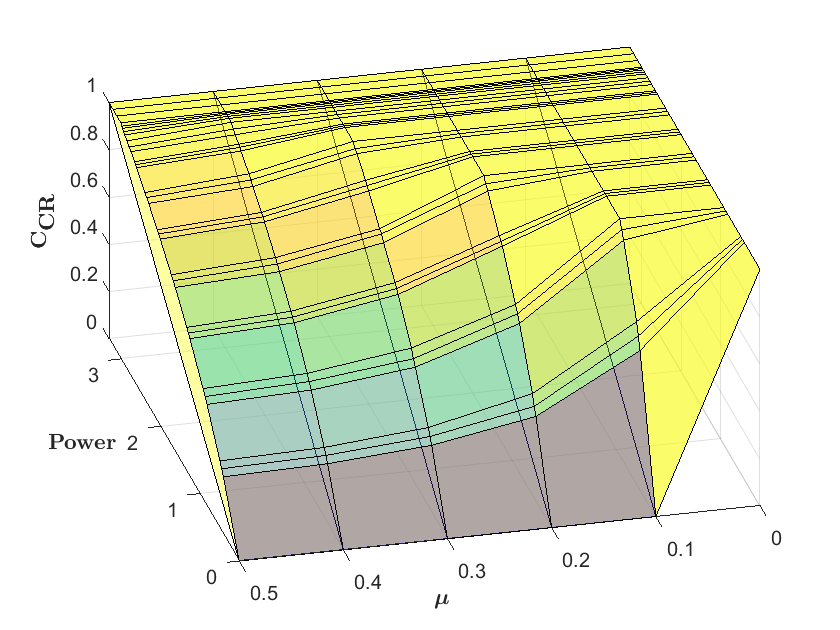
Next, we generate a three-dimensional plot of the common randomness capacity as a function of both the power and the parameter μ\mu. This is illustrated in Fig. 7.

Refer to caption
Figure 7: CR capacity in function of the power and the parameter μ\mu for a noise variance σ2=1.\sigma^{2}=1.

We consider first the specific case when μ=0\mu=0. Clearly, for μ=0\mu=0, it holds that Y=XY=X. Therefore, no communication over the channel is required to achieve the maximal amount of common randomness equal to H⁡(X)H(X). This is numerically verified in Fig. 6 and Fig. 7, where for μ=0\mu=0 and P=0P=0 the common randomness capacity is equal to H⁡(X)=1.H(X)=1. However, for 0<μ≤120<\mu\leq\frac{1}{2}, a communication over the channel is necessary to generate common randomness between the two terminals (CC​R​(0)=0CLOSE(C_{CR}\left(0\right)=0 for 0<μ≤120<\mu\leq\frac{1}{2}). This is due to the fact that XX and YY have an indecomposable joint distribution [1] for 0<μ≤120<\mu\leq\frac{1}{2}. Furthermore, the higher the parameter μ\mu is, the less correlated the sources are. As a result, we need to investigate more power in order to achieve the same amount of common randomness obtained for lower values of μ\mu. This is clearly observable in Fig. 6. For instance, for μ=0.2\mu=0.2, the common randomness capacity is equal to 0.86 for P≈1.33P\thickapprox 1.33, whereas, for μ=0.5\mu=0.5, the same amount of common randomness is achieved for P≈2.34P\thickapprox 2.34.

3.2 MIMO Case

We now focus on the second scenario depicted in Fig. 2, where the communication is over a MIMO Gaussian channel with the power constraint defined in (8).

Proposition 2

For the model in Fig. 2, the CR capacity CC​R​(P,NT×NR)C_{CR}(P,N_{T}\times N_{R}) is equal:

CC​R​(P,NT×NR)=maxUU  ​@​a​r​r​o​wX  ​@​a​r​r​o​wYI⁡(U,X)−I⁡(U,Y)≤C⁡(P,NT×NR)​I​(U,X).C_{CR}(P,N_{T}\times N_{R})=\underset{\begin{subarray}{c}U\\ {\begin{subarray}{c}U\mathrel{\vphantom{\rightarrow}\mathchoice{\circle{0.0}{@}}{\circle{0.0}{@}}{\circle{0.0}{@}}{\circle{0.0}{@}}arrow}{X}\mathrel{\vphantom{\rightarrow}\mathchoice{\circle{0.0}{@}}{\circle{0.0}{@}}{\circle{0.0}{@}}{\circle{0.0}{@}}arrow}{Y}\\ I(U;X)-I(U;Y)\leq C(P,N_{T}\times N_{R})\end{subarray}}\end{subarray}}{\max}I(U;X).

Direct Proof

𝑻~\boldsymbol{\tilde{T}}𝐕\mathbf{V}𝐕𝖧\mathbf{V}^{\mathsf{H}}×\times×\times𝐔\mathbf{U}𝐔𝖧\mathbf{U}^{\mathsf{H}}𝒁~\boldsymbol{\tilde{Z}}λ1\lambda_{1}λNmin\lambda_{N_{\text{min}}}++𝝃~\boldsymbol{\tilde{\xi}}𝑻\boldsymbol{T}𝒁\boldsymbol{Z}pre-processingpost-processing⋮\vdotschannel
Figure 8: Decomposition of the MIMO channel into NminN_{\text{min}} parallel channels through SVD.
Proof

The capacity C⁡(P,NT×NR)C(P,N_{T}\times N_{R}) can be computed by converting the MIMO channel into parallel, independent and scalar Gaussian sub-channels. This conversion is based on the following singular value decomposition (SVD) of the channel matrix 𝐇\mathbf{H}:

𝐇=𝐔​𝚲​𝐕𝖧,\mathbf{H}=\mathbf{U}\mathbf{\Lambda}\mathbf{V}^{\mathsf{H}},

where 𝐔∈ℂNR×NR\mathbf{U}\in\mathbb{C}^{N_{R}\times N_{R}} and 𝐕∈ℂNT×NT\mathbf{V}\in\mathbb{C}^{N_{T}\times N_{T}} are unitary matrices. 𝚲∈ℂNR×NT\mathbf{\Lambda}\in\mathbb{C}^{N_{R}\times N_{T}} is a diagonal matrix, whose diagonal elements λ1≥λ2≥⋯≥λNmin\lambda_{1}\geq\lambda_{2}\geq\cdots\geq\lambda_{N_{\text{min}}} are the ordered singular values of the channel matrix 𝐇\mathbf{H}. We denote with NminN_{\text{min}} the rank of 𝐇\mathbf{H}, Nmin≔min⁡(NT,NR)N_{\text{min}}\coloneqq\min(N_{T},N_{R}). If we multiply (10) with the unitary matrix 𝐔𝖧\mathbf{U}^{\mathsf{H}}, we then obtain

𝐔𝖧​𝒁⏟≔𝒁~=𝐔𝖧​𝐔​𝚲​𝐕𝖧​𝑻⏟≔𝑻~+𝐔𝖧​𝝃⏟≔𝝃~.\underbrace{\mathbf{U}^{\mathsf{H}}\boldsymbol{Z}}_{\coloneqq\tilde{\boldsymbol{Z}}}=\mathbf{U}^{\mathsf{H}}\mathbf{U}\mathbf{\Lambda}\underbrace{\mathbf{V}^{\mathsf{H}}\boldsymbol{T}}_{\coloneqq\tilde{\boldsymbol{T}}}+\underbrace{\mathbf{U}^{\mathsf{H}}\boldsymbol{\xi}}_{\coloneqq\tilde{\boldsymbol{\xi}}}.

It can easily be checked that 𝝃~\tilde{\boldsymbol{\xi}} has the same distribution as 𝝃\boldsymbol{\xi} [34], i.e., 𝝃~∼𝒩ℂ​(𝟎NR,σ2​𝐈NR),\tilde{\boldsymbol{\xi}}\sim\mathcal{N}_{\mathbb{C}}(\boldsymbol{0}_{N_{R}},\sigma^{2}\mathbf{I}_{N_{R}}), and we have

𝔼⁡[𝑻~𝖧​𝑻~]=𝔼⁡[𝑻𝖧​𝐕𝐕𝖧​𝑻]=𝔼⁡[𝑻𝖧​𝑻].\mathbb{E}[\tilde{\boldsymbol{T}}^{\mathsf{H}}\tilde{\boldsymbol{T}}]=\mathbb{E}[\boldsymbol{T}^{\mathsf{H}}\mathbf{V}\mathbf{V}^{\mathsf{H}}\boldsymbol{T}]=\mathbb{E}[\boldsymbol{T}^{\mathsf{H}}\boldsymbol{T}].

We obtain the NminN_{\text{min}} independent scalar Gaussian channels depicted in Fig. 8

Z~ℓ=λℓ​T~ℓ+ξ~ℓℓ=1​…​Nmin.\displaystyle\tilde{Z}_{\ell}=\lambda_{\ell}\tilde{T}_{\ell}+\tilde{\xi}_{\ell}\ \ \ell=1\dots N_{\text{min}}.

The SVD can be interpreted as a pre-processing (multiplication with 𝐕\mathbf{V}) and a post-processing (multiplication with 𝐔H\mathbf{U}^{H}). The optimization problem in (11) is reduced to [35]

C⁡(P,NT×NR)=max⁡∑ℓ=1NminP~1​…​P~Nmin⁡log⁡(1+λℓ2σ2​Pℓ~),\displaystyle C(P,N_{T}\times N_{R})=\max_{\tilde{P}_{1}\dots\tilde{P}_{N_{\text{min}}}}\sum_{\ell=1}^{N_{\text{min}}}\log\left(1+\frac{\lambda_{\ell}^{2}}{\sigma^{2}}\tilde{P_{\ell}}\right),
s.t.​∑ℓ=1NminPℓ~≤P​and​Pℓ~≥0ℓ=1​…​Nmin.\displaystyle\text{s.t.}\sum_{\ell=1}^{N_{\text{min}}}\tilde{P_{\ell}}\leq P\ \text{and}\ \tilde{P_{\ell}}\geq 0\ \ \ell=1\dots N_{\text{min}}.

It holds that

C⁡(P,NT×NR)=∑ℓ=1NminC⁡(P~ℓ),\displaystyle C(P,N_{T}\times N_{R})=\sum_{\ell=1}^{N_{\text{min}}}C(\tilde{P}_{\ell}),

where the capacity of each sub-channel is expressed as

C⁡(P~ℓ)=log⁡(1+λℓ2σ2​Pℓ~)ℓ=1​…​Nmin.\displaystyle C(\tilde{P}_{\ell})=\log\left(1+\frac{\lambda_{\ell}^{2}}{\sigma^{2}}\tilde{P_{\ell}}\right)\ \ \ell=1\dots N_{\text{min}}.

The power Pℓ~\tilde{P_{\ell}} is called the waterfilling rule [36] and it is expressed as follows:

Pℓ~=max⁡(0,κ−σ2λℓ)​ℓ=1​…​Nmin,\tilde{P_{\ell}}=\max\left(0,\kappa-\frac{\sigma^{2}}{\lambda_{\ell}}\right)\ \ell=1\dots N_{\text{min}},

where κ\kappa is the waterfilling level.

By Proposition 1, we have for ℓ=1​…​Nmin.\ell=1\ldots N_{\text{min}}.

CC​R​(Pℓ~)=maxUℓUℓ  ​@​a​r​r​o​wX  ​@​a​r​r​o​wYI⁡(Uℓ,X)−I⁡(Uℓ,Y)≤C⁡(P~ℓ)​I​(Uℓ,X).\displaystyle C_{CR}(\tilde{P_{\ell}})=\underset{\begin{subarray}{c}U_{\ell}\\ {\begin{subarray}{c}U_{\ell}\mathrel{\vphantom{\rightarrow}\mathchoice{\circle{0.0}{@}}{\circle{0.0}{@}}{\circle{0.0}{@}}{\circle{0.0}{@}}arrow}{X}\mathrel{\vphantom{\rightarrow}\mathchoice{\circle{0.0}{@}}{\circle{0.0}{@}}{\circle{0.0}{@}}{\circle{0.0}{@}}arrow}{Y}\\ I(U_{\ell};X)-I(U_{\ell};Y)\leq C(\tilde{P}_{\ell})\end{subarray}}\end{subarray}}{\max}I(U_{\ell};X).

Since we may lose information through processing, it holds that

CC​R​(P,NT×NR)\displaystyle C_{CR}(P,N_{T}\times N_{R})
≥∑ℓ=1NminCC​R​(P~ℓ)\displaystyle\geq\sum_{\ell=1}^{N_{\text{min}}}C_{CR}(\tilde{P}_{\ell})
=∑ℓ=1NminmaxUℓUℓ  ​@​a​r​r​o​wX  ​@​a​r​r​o​wYI⁡(Uℓ,X)−I⁡(Uℓ,Y)≤C⁡(P~ℓ)​I​(Uℓ,X)\displaystyle=\sum_{\ell=1}^{N_{\text{min}}}\underset{\begin{subarray}{c}U_{\ell}\\ {\begin{subarray}{c}U_{\ell}\mathrel{\vphantom{\rightarrow}\mathchoice{\circle{0.0}{@}}{\circle{0.0}{@}}{\circle{0.0}{@}}{\circle{0.0}{@}}arrow}{X}\mathrel{\vphantom{\rightarrow}\mathchoice{\circle{0.0}{@}}{\circle{0.0}{@}}{\circle{0.0}{@}}{\circle{0.0}{@}}arrow}{Y}\\ I(U_{\ell};X)-I(U_{\ell};Y)\leq C(\tilde{P}_{\ell})\end{subarray}}\end{subarray}}{\max}I(U_{\ell};X)
=∑ℓ=1NminmaxU1​…​UNminUℓ  ​@​a​r​r​o​wX  ​@​a​r​r​o​wY​ℓ=1​…​NminI⁡(Uℓ,X)−I⁡(Uℓ,Y)≤C⁡(P~ℓ)​ℓ=1​…​Nmin​I​(Uℓ,X)\displaystyle=\sum_{\ell=1}^{N_{\text{min}}}\underset{\begin{subarray}{c}U_{1}\ldots U_{N_{\text{min}}}\\ {\begin{subarray}{c}U_{\ell}\mathrel{\vphantom{\rightarrow}\mathchoice{\circle{0.0}{@}}{\circle{0.0}{@}}{\circle{0.0}{@}}{\circle{0.0}{@}}arrow}{X}\mathrel{\vphantom{\rightarrow}\mathchoice{\circle{0.0}{@}}{\circle{0.0}{@}}{\circle{0.0}{@}}{\circle{0.0}{@}}arrow}{Y}\ \ell=1\ldots N_{\text{min}}\\ I(U_{\ell};X)-I(U_{\ell};Y)\leq C(\tilde{P}_{\ell})\ \ell=1\ldots N_{\text{min}}\end{subarray}}\end{subarray}}{\max}I(U_{\ell};X)
≥maxU1​…​UNminUℓ  ​@​a​r​r​o​wX  ​@​a​r​r​o​wY​ℓ=1​…​NminI⁡(Uℓ,X)−I⁡(Uℓ,Y)≤C⁡(P~ℓ)​ℓ=1​…​Nmin​∑ℓ=1NminI⁡(Uℓ,X)\displaystyle\geq\underset{\begin{subarray}{c}U_{1}\ldots U_{N_{\text{min}}}\\ {\begin{subarray}{c}U_{\ell}\mathrel{\vphantom{\rightarrow}\mathchoice{\circle{0.0}{@}}{\circle{0.0}{@}}{\circle{0.0}{@}}{\circle{0.0}{@}}arrow}{X}\mathrel{\vphantom{\rightarrow}\mathchoice{\circle{0.0}{@}}{\circle{0.0}{@}}{\circle{0.0}{@}}{\circle{0.0}{@}}arrow}{Y}\ \ell=1\ldots N_{\text{min}}\\ I(U_{\ell};X)-I(U_{\ell};Y)\leq C(\tilde{P}_{\ell})\ \ell=1\ldots N_{\text{min}}\end{subarray}}\end{subarray}}{\max}\sum_{\ell=1}^{N_{\text{min}}}I(U_{\ell};X)
≥maxU1​…​UNminI⁡(Uℓ,X)−I⁡(Uℓ,Y)≤C⁡(P~ℓ)​ℓ=1​…​NminUℓ​independent of​(X,Y),ℓ=1​…,NminUℓ,ℓ=1​…,Nmin,pairwise independent∑ℓ=1NminI⁡(Uℓ,X)−∑ℓ=1NminI⁡(Uℓ,Y)≤∑ℓ=1NminC⁡(P~ℓ)​∑ℓ=1NminI⁡(Uℓ,X)\displaystyle\geq\underset{\begin{subarray}{c}U_{1}\ldots U_{N_{\text{min}}}\\ {\begin{subarray}{c}I(U_{\ell};X)-I(U_{\ell};Y)\leq C(\tilde{P}_{\ell})\ \ell=1\ldots N_{\text{min}}\end{subarray}}\\ U_{\ell}\ \text{independent of}\ (X,Y),\ \ell=1\ldots,N_{\text{min}}\\ U_{\ell},\ \ell=1\ldots,N_{\text{min}},\ \text{pairwise independent}\\ \sum_{\ell=1}^{N_{\text{min}}}I(U_{\ell};X)-\sum_{\ell=1}^{N_{\text{min}}}I(U_{\ell};Y)\leq\sum_{\ell=1}^{N_{\text{min}}}C(\tilde{P}_{\ell})\end{subarray}}{\max}\sum_{\ell=1}^{N_{\text{min}}}I(U_{\ell};X)
=(a)​maxVV  ​@​a​r​r​o​wX  ​@​a​r​r​o​wYI⁡(V,X)−I⁡(V,Y)≤∑ℓ=1NminC⁡(P~ℓ)​I​(V,X)\displaystyle\overset{(a)}{=}\underset{\begin{subarray}{c}V\\ {\begin{subarray}{c}V\mathrel{\vphantom{\rightarrow}\mathchoice{\circle{0.0}{@}}{\circle{0.0}{@}}{\circle{0.0}{@}}{\circle{0.0}{@}}arrow}{X}\mathrel{\vphantom{\rightarrow}\mathchoice{\circle{0.0}{@}}{\circle{0.0}{@}}{\circle{0.0}{@}}{\circle{0.0}{@}}arrow}{Y}\\ I(V;X)-I(V;Y)\leq\sum_{\ell=1}^{N_{\text{min}}}C(\tilde{P}_{\ell})\end{subarray}}\end{subarray}}{\max}I(V;X)
=maxVV  ​@​a​r​r​o​wX  ​@​a​r​r​o​wYI⁡(V,X)−I⁡(V,Y)≤C⁡(P,NT×NR)​I​(V,X),\displaystyle=\underset{\begin{subarray}{c}V\\ {\begin{subarray}{c}V\mathrel{\vphantom{\rightarrow}\mathchoice{\circle{0.0}{@}}{\circle{0.0}{@}}{\circle{0.0}{@}}{\circle{0.0}{@}}arrow}{X}\mathrel{\vphantom{\rightarrow}\mathchoice{\circle{0.0}{@}}{\circle{0.0}{@}}{\circle{0.0}{@}}{\circle{0.0}{@}}arrow}{Y}\\ I(V;X)-I(V;Y)\leq C(P,N_{T}\times N_{R})\end{subarray}}\end{subarray}}{\max}I(V;X), (28)

where (a)(a) follows from defining VV such that Uℓ  ​@​a​r​r​o​wV  ​@​a​r​r​o​wX  ​@​a​r​r​o​wY,ℓ=1​…​NminU_{\ell}\mathrel{\vphantom{\rightarrow}\mathchoice{\circle{0.0}{@}}{\circle{0.0}{@}}{\circle{0.0}{@}}{\circle{0.0}{@}}arrow}{V}\mathrel{\vphantom{\rightarrow}\mathchoice{\circle{0.0}{@}}{\circle{0.0}{@}}{\circle{0.0}{@}}{\circle{0.0}{@}}arrow}{X}\mathrel{\vphantom{\rightarrow}\mathchoice{\circle{0.0}{@}}{\circle{0.0}{@}}{\circle{0.0}{@}}{\circle{0.0}{@}}arrow}{Y},\ \ell=1\ldots N_{\text{min}}, with I⁡(V,X)=∑ℓ=1NminI⁡(Uℓ,X)I(V;X)=\sum_{\ell=1}^{N_{\text{min}}}I(U_{\ell};X) and I⁡(V,Y)=∑ℓ=1NminI⁡(Uℓ,Y)I(V;Y)=\sum_{\ell=1}^{N_{\text{min}}}I(U_{\ell};Y). Here, UℓU_{\ell}, ℓ=1​…​Nmin\ell=1\ldots N_{\text{min}}, satisfy the following constraints:

  1. 1.

    Each Uℓ,ℓ=1​…​NminU_{\ell},\ \ell=1\ldots N_{\text{min}} is independent of (X,Y).(X,Y).

  2. 2.

    I⁡(Uℓ,X)−I⁡(Uℓ,Y)≤C⁡(P~ℓ)for​ℓ=1​…​Nmin.I(U_{\ell};X)-I(U_{\ell};Y)\leq C(\tilde{P}_{\ell})\quad\text{for}\ \ell=1\ldots N_{\text{min}}.

  3. 3.

    UℓU_{\ell}, ℓ=1​…​Nmin\ell=1\ldots N_{\text{min}}, are pairwise independent.

The existence of such VV is proved in the appendix.

Converse Part:

The converse proof for the MIMO case is analogous to the converse proof for the SISO case.

Remark 8

The signal processing presented in Section 3.2 is optimal in the sense that with this processing, one can demonstrate the achievability of the common randomness capacity over the MIMO Gaussian channel.

Remark 9

Since C⁡(P,NT×NR)≥C⁡(P)C(P,N_{T}\times N_{R})\geq C(P), it follows from Proposition 1 and Proposition 2 that:

CC​R​(P,NT×NR)≥CC​R​(P).\displaystyle C_{CR}(P,N_{T}\times N_{R})\geq C_{CR}(P).

Intuitively, because the MIMO channel has a higher capacity than the SISO channel, the amount of information that can be reliably transmitted is greater. Consequently, by communicating over the MIMO channel, Terminals AA and BB can generate a greater amount of common randomness.

4 Application of Common Randomness: Secure Identification

In this section, we explore a significant application of CR generation: the identification paradigm. Unlike transmission, it appears that the resource CR can enhance the identification capacity of channels. We introduce a coding scheme for CR-assisted secure identification and prove a lower bound on the secure identification capacity within this setting, as illustrated in Proposition 3.

Proposition 3

Let CS​I​Dc​(g,g′,P)C_{SID}^{c}(g,g^{\prime},P) and CS​(g,g′,P)C_{S}(g,g^{\prime},P), respectively, be the secure identification capacity and the secrecy capacity for the model in Fig. 4, respectively. It holds that

if​CS​(g,g′,P)>0​then\text{if}\ C_{S}(g,g^{\prime},P)>0\ \text{then}

CS​I​Dc​(g,g′,P)≥maxUU  ​@​a​r​r​o​wX  ​@​a​r​r​o​wYI⁡(U,X)−I⁡(U,Y)≤C⁡(g,P)​I​(U,X).C_{SID}^{c}(g,g^{\prime},P)\geq\underset{\begin{subarray}{c}U\\ {\begin{subarray}{c}U\mathrel{\vphantom{\rightarrow}\mathchoice{\circle{0.0}{@}}{\circle{0.0}{@}}{\circle{0.0}{@}}{\circle{0.0}{@}}arrow}{X}\mathrel{\vphantom{\rightarrow}\mathchoice{\circle{0.0}{@}}{\circle{0.0}{@}}{\circle{0.0}{@}}{\circle{0.0}{@}}arrow}{Y}\\ I(U;X)-I(U;Y)\leq C(g,P)\end{subarray}}\end{subarray}}{\max}I(U;X).
Remark 10

Consider in particular the case when C⁡(g,P)≥H⁡(X|Y)C(g,P)\geq H(X|Y). Then, it follows from Proposition 3 that CS​I​Dc​(g,g′,P)≥H⁡(X)C_{SID}^{c}(g,g^{\prime},P)\geq H(X) as long as CS​(g,g′,P)>0C_{S}(g,g^{\prime},P)>0.

Proof

Given a DMMS PX​YP_{XY}, Alice observes the outputs XnX^{n} and Bob observes the outputs Yn.Y^{n}. Alice generates a random variable KK with alphabet 𝒦={1​…​M′},\mathcal{K}=\{1\dots M^{\prime}\}, such that K=Φ⁡(Xn).K=\Phi(X^{n}). To send a message ii, we prepare a set of coloring-functions or mappings EiE_{i} known by the sender and the receiver.

Ei\displaystyle E_{i} :𝒦⟶{1,…,M′′}\displaystyle\colon\mathcal{K}\longrightarrow\{1,\ldots,M^{\prime\prime}\}
:K⏟coloring↦Ei​(K).⏟color\displaystyle\colon\underbrace{K}_{\text{coloring}}\mapsto\underbrace{E_{i}(K).}_{\text{color}}

XnX^{n} is encoded to a sequence TnT^{n} using an error correcting code, then Ei​(K)E_{i}(K) is encoded to a sequence T⌈n⌉T^{\lceil\sqrt{n}\rceil} using a wiretap code as proposed in [37]. The sequence TmT^{m}, obtained by concatenating TnT^{n} and T⌈n⌉T^{\lceil\sqrt{n}\rceil}, where m=n+⌈n⌉m=n+\lceil\sqrt{n}\rceil as depicted in Fig. 9, fulfills the power constraint:

𝔼⁡[Ti2]≤P∀i=1​…​m.\mathbb{E}[T_{i}^{2}]\leq P\quad\forall i=1\dots m.
𝑻n\boldsymbol{T}^{n} u′′u^{\prime\prime}nn⌈n⌉\lceil\sqrt{n}\rceilmmAliceXnX^{n}u1′′u^{\prime\prime}_{1}u2′′u^{\prime\prime}_{2}  uM′′′′u^{\prime\prime}_{M^{\prime\prime}}𝒞′′={(uℓ′′,𝒟ℓ′′),ℓ∈{1,…,M′′}}\mathcal{C}^{\prime\prime}=\{(u^{\prime\prime}_{\ell},\mathcal{D}^{\prime\prime}_{\ell}),\ell\in\{1,\ldots,M^{\prime\prime}\}\}wiretap code|𝒞′′|=⌈2n​ϵ⌉|\mathcal{C}^{\prime\prime}|=\lceil 2^{\sqrt{n}\epsilon}\rceilRefer to caption
Figure 9: Coding scheme.

TmT^{m} is sent over the Wiretap channel.

Bob generates L=Ψ⁡(Yn,Zn)L=\Psi(Y^{n},Z^{n}) such that Pr[K≠L]\text{Pr}[K\neq L] is low. Since we have used a wiretap code in the second part, Bob, interested in i′i^{\prime}, can identify whether the message of interest was sent or not. We choose the rate of the first code to be approximately equal to the capacity of the channel to the legitimate receiver so that Bob can identify the message at a rate approximately equal to C⁡(g,P),C(g,P), the transmission capacity of the main channel, without paying a price for the identification task. Although Eve can decode with low error probability the sequence TnT^{n}, she cannot, with this setting, identify the color, i.e., the second fundamental part of the sent codeword, even if she knows the correlation between the sources. Thus, the wiretapper cannot identify the message ii. For more details regarding the proof, we refer the reader to [25]. Let us denote the CR capacity for this model by CC​R​(g,P).C_{CR}(g,P). Then, by applying the Transformator-Lemma [38][39], it holds that

CS​I​Dc​(g,g′,P)≥CC​R​(g,P)​if​CS​(g,g′,P)>0.\displaystyle C_{SID}^{c}(g,g^{\prime},P)\geq C_{CR}(g,P)\hskip 8.5359pt\text{if}\ C_{S}(g,g^{\prime},P)>0.

In addition, it holds by Proposition 1 that

CC​R​(g,P)=maxUU  ​@​a​r​r​o​wX  ​@​a​r​r​o​wYI⁡(U,X)−I⁡(U,Y)≤C⁡(g,P)​I​(U,X).\displaystyle C_{CR}(g,P)=\underset{\begin{subarray}{c}U\\ {\begin{subarray}{c}U\mathrel{\vphantom{\rightarrow}\mathchoice{\circle{0.0}{@}}{\circle{0.0}{@}}{\circle{0.0}{@}}{\circle{0.0}{@}}arrow}{X}\mathrel{\vphantom{\rightarrow}\mathchoice{\circle{0.0}{@}}{\circle{0.0}{@}}{\circle{0.0}{@}}{\circle{0.0}{@}}arrow}{Y}\\ I(U;X)-I(U;Y)\leq C(g,P)\end{subarray}}\end{subarray}}{\max}I(U;X).
Remark 11

It has recently been proven in [25] that the secure identification capacity with randomized encoding is equal to the capacity of the channel to the legitimate receiver C⁡(g,P)C(g,P), provided that the secrecy capacity is strictly positive. As long as PP is chosen to satisfy C⁡(g,P)≤H⁡(X)C(g,P)\leq H(X), the lower bound in Proposition 3 may exceed the capacity of the main channel. Let us reconsider the example of binary sources presented in Example 1. It is observed in Fig. 10 that we can achieve a performance gain of at least 0.2780.278 for P≈1.72P\approx 1.72, μ=0.2\mu=0.2, and σ2=1\sigma^{2}=1.

000.20.20.40.40.60.60.80.8111.21.21.41.41.61.61.81.8222.22.22.42.42.62.62.82.833000.10.10.20.20.30.30.40.40.50.50.60.60.70.70.80.80.90.911PowerSecure Identification CapacityCapacity of secure identificationin presence of local randomnessLower bound on CR-assistedsecure identification capacity
Figure 10: Comparison of the lower bound on CR-assisted secure identification to the capacity of secure identification with randomized encoding for a noise variance σ2=1\sigma^{2}=1, for the correlated sources presented in Example 1 with μ=0.2.\mu=0.2.

Furthermore, if we consider identification over Gaussian channels without the availability of CR as a resource and with deterministic encoding, then, in this case, the identification capacity, measured on the log-log scale as already introduced in Definition 4, is equal to zero. This implies that the secure identification capacity for this communication scenario is also always equal to zero. This demonstrates, as already noted in Remark 4, that in contrast to transmission, the resource CR allows for a significant performance gain in the identification task.

Remark 12

Clearly, we can proceed analogously to derive a lower bound for CR-assisted secure identification capacity over MIMO GWCs.

5 Conclusions

We studied the problem of CR generation over single-user SISO and MIMO Gaussian channels due to their practical relevance in various communication scenarios, such as satellite and deep space communication links, wired and wireless communications, etc. We provided a single-letter characterization of the CR capacity for both scenarios along with rigorous proofs. Additionally, we demonstrated that through CR generation, significant performance gains could be achieved in Post-Shannon communication tasks, which could be advantageous in numerous new applications, including machine-to-machine and human-to-machine systems, as well as the tactile internet. Specifically, we proposed a coding scheme for secure identification over the GWC with CR available as a resource and established a lower bound on the secure identification capacity within this framework. This lower bound may exceed the transmission capacity of the main channel, which is equal to the secure identification capacity in the case of randomized encoding, provided the secrecy capacity is strictly positive. As a future work, we suggest investigating the impact of antenna correlation on the CR capacity of MIMO Gaussian channels. Subsequent research could focus on providing a single-letter characterization of the CR-assisted secure identification capacity of the GWC and exploring CR-assisted identification for continuous-time channels.

Appendix 0.A Appendix

0.A.1 Proof of the Existence of a random variable VV as defined in (28)

Proof

We want to show that a random variable VV exists such that Uℓ  ​@​a​r​r​o​wV  ​@​a​r​r​o​wX  ​@​a​r​r​o​wY,ℓ=1​…​NminU_{\ell}\mathrel{\vphantom{\rightarrow}\mathchoice{\circle{0.0}{@}}{\circle{0.0}{@}}{\circle{0.0}{@}}{\circle{0.0}{@}}arrow}{V}\mathrel{\vphantom{\rightarrow}\mathchoice{\circle{0.0}{@}}{\circle{0.0}{@}}{\circle{0.0}{@}}{\circle{0.0}{@}}arrow}{X}\mathrel{\vphantom{\rightarrow}\mathchoice{\circle{0.0}{@}}{\circle{0.0}{@}}{\circle{0.0}{@}}{\circle{0.0}{@}}arrow}{Y},\ \ell=1\ldots N_{\text{min}} with I⁡(V,X)=∑ℓ=1NminI⁡(Uℓ,X)I(V;X)=\sum_{\ell=1}^{N_{\text{min}}}I(U_{\ell};X) and I⁡(V,Y)=∑ℓ=1NminI⁡(Uℓ,Y)I(V;Y)=\sum_{\ell=1}^{N_{\text{min}}}I(U_{\ell};Y), where Uℓ,ℓ=1​…​Nmin,U_{\ell},\ell=1\ldots N_{\text{min}}, satisfy the following constraints:

  1. 1.

    Each Uℓ,ℓ=1​…​Nmin,U_{\ell},\ \ell=1\ldots N_{\text{min}}, is independent of (X,Y).(X,Y).

  2. 2.

    I⁡(Uℓ,X)−I⁡(Uℓ,Y)≤C⁡(P~ℓ)ℓ=1​…​NminI(U_{\ell};X)-I(U_{\ell};Y)\leq C(\tilde{P}_{\ell})\quad\ell=1\ldots N_{\text{min}}

  3. 3.

    UℓU_{\ell}, ℓ=1​…​Nmin\ell=1\ldots N_{\text{min}}, are pairwise independent

It suffices to consider V=U1​…​UNminV=U_{1}\ldots U_{N_{\text{min}}}. Then it holds that

I⁡(V,X)\displaystyle I(V;X) =I⁡(U1​…​UNmin,X)\displaystyle=I(U_{1}\ldots U_{N_{\text{min}}};X)
=∑ℓ=1NminI⁡(Uℓ;X|U1​…​Uℓ−1)\displaystyle=\sum_{\ell=1}^{N_{\text{min}}}I(U_{\ell};X|U_{1}\ldots U_{\ell-1})
=(a)​∑ℓ=1NminI⁡(Uℓ,X),\displaystyle\overset{(a)}{=}\sum_{\ell=1}^{N_{\text{min}}}I(U_{\ell};X),

where (a)(a) follows because Uℓ,U_{\ell}, ℓ=1​…​Nmin,\ell=1\ldots N_{\text{min}}, are pairwise independent and because each Uℓ,U_{\ell}, ℓ=1​…​Nmin,\ell=1\ldots N_{\text{min}}, is independent of X.X. Analogously, it holds that I⁡(V,Y)=∑ℓ=1NminI⁡(Uℓ,Y)I(V;Y)=\sum_{\ell=1}^{N_{\text{min}}}I(U_{\ell};Y).
 
The Markov chain Uℓ  ​@​a​r​r​o​wV  ​@​a​r​r​o​wX  ​@​a​r​r​o​wY,U_{\ell}\mathrel{\vphantom{\rightarrow}\mathchoice{\circle{0.0}{@}}{\circle{0.0}{@}}{\circle{0.0}{@}}{\circle{0.0}{@}}arrow}{V}\mathrel{\vphantom{\rightarrow}\mathchoice{\circle{0.0}{@}}{\circle{0.0}{@}}{\circle{0.0}{@}}{\circle{0.0}{@}}arrow}{X}\mathrel{\vphantom{\rightarrow}\mathchoice{\circle{0.0}{@}}{\circle{0.0}{@}}{\circle{0.0}{@}}{\circle{0.0}{@}}arrow}{Y}, ℓ=1​…​Nmin,\ell=1\ldots N_{\text{min}}, is satisfied since for ℓ=1​…​Nmin,\ell=1\ldots N_{\text{min}}, we have

ℙ[Y=y|X=x,V=v,Uℓ=uℓ]\displaystyle\mathbb{P}[Y=y|X=x,V=v,U_{\ell}=u_{\ell}]
=(a)ℙ[Y=y|X=x,V=v]\displaystyle\overset{(a)}{=}\mathbb{P}[Y=y|X=x,V=v]
=ℙ[Y=y|X=x,U=u1,U2=u2,…,UNmin=uNmin]\displaystyle=\mathbb{P}[Y=y|X=x,U=u_{1},U_{2}=u_{2},\ldots,{U_{N}}_{\text{min}}={u_{N}}_{\text{min}}]
=(b)​ℙ​[Y=y|X=x],\displaystyle\overset{(b)}{=}\mathbb{P}[Y=y|X=x],

where (a)(a) follows because V=U1​…​UNminV=U_{1}\ldots U_{N_{\text{min}}} and where (b)(b) follows because each UℓU_{\ell} is independent of (X,Y).(X,Y).

0.A.2 Proof of the Non-Convexity of g0​(𝜽)g_{0}\left(\boldsymbol{\theta}\right)

It holds that

g0​(𝜽)\displaystyle g_{0}\left(\boldsymbol{\theta}\right) =−I⁡(U,X)\displaystyle=-I(U;X)
=−H⁡(X)−H⁡(U)+H⁡(X​U),\displaystyle=-H(X)-H(U)+H(XU),

which yields

∂g0​(𝜽)∂PU​X​(u,x)=∂H⁡(X​U)∂PU​X​(u,x)−∂H⁡(U)∂PU​X​(u,x).\frac{\partial g_{0}\left(\boldsymbol{\theta}\right)}{\partial P_{UX}\left(u,x\right)}=\frac{\partial H(XU)}{\partial P_{UX}\left(u,x\right)}-\frac{\partial H(U)}{\partial P_{UX}\left(u,x\right)}.

On one side, we have

H⁡(U)\displaystyle H(U)
=−∑u′∈𝒰​PU​(u′)​log⁡(PU​(u′))\displaystyle=-\underset{u^{\prime}\in\mathcal{U}}{\sum}P_{U}\left(u^{\prime}\right)\log\left(P_{U}\left(u^{\prime}\right)\right)
=−∑u′∈𝒰​(∑x′∈𝒳​PU​X​(u′,x′))​log⁡(∑x′∈𝒳​PU​X​(u′,x′))\displaystyle=-\underset{u^{\prime}\in\mathcal{U}}{\sum}\left(\underset{x^{\prime}\in\mathcal{X}}{\sum}P_{UX}\left(u^{\prime},x^{\prime}\right)\right)\log\left(\underset{x^{\prime}\in\mathcal{X}}{\sum}P_{UX}\left(u^{\prime},x^{\prime}\right)\right)

yielding

∂H⁡(U)∂PU​X​(u,x)=−[log⁡(∑x′∈𝒳​PU​X​(u,x′))+1ln⁡(2)].\frac{\partial H(U)}{\partial P_{UX}\left(u,x\right)}=-\left[\log\left(\underset{x^{\prime}\in\mathcal{X}}{\sum}P_{UX}\left(u,x^{\prime}\right)\right)+\frac{1}{\ln(2)}\right].

On the other side, we have

H⁡(U​X)=−∑u′∈𝒰,x′∈𝒳​PU​X​(u′,x′)​log⁡(PU​X​(u′,x′))H(UX)=-\underset{u^{\prime}\in\mathcal{U},x^{\prime}\in\mathcal{X}}{\sum}P_{UX}\left(u^{\prime},x^{\prime}\right)\log\left(P_{UX}\left(u^{\prime},x^{\prime}\right)\right)

yielding

∂H⁡(U​X)∂PU​X​(u,x)=−[log⁡(PU​X​(u,x))+1ln⁡(2)].\frac{\partial H(UX)}{\partial P_{UX}\left(u,x\right)}=-\left[\log\left(P_{UX}\left(u,x\right)\right)+\frac{1}{\ln(2)}\right].

Thus, we obtain

∂g0​(𝜽)∂PU​X​(u,x)=log⁡(∑x′∈𝒳​PU​X​(u,x′)PU​X​(u,x)).\frac{\partial g_{0}\left(\boldsymbol{\theta}\right)}{\partial P_{UX}\left(u,x\right)}=\log\left(\frac{\underset{x^{\prime}\in\mathcal{X}}{\sum}P_{UX}\left(u,x^{\prime}\right)}{P_{UX}\left(u,x\right)}\right). (29)

As a result,

∂2g0​(𝜽)∂2PU​X​(u,x)=PU​X​(u,x)−∑x′∈𝒳​PU​X​(u,x′)PU​X​(u,x)​∑x′∈𝒳​PU​X​(u,x′)≤0\frac{\partial^{2}g_{0}\left(\boldsymbol{\theta}\right)}{\partial^{2}P_{UX}\left(u,x\right)}=\frac{P_{UX}\left(u,x\right)-\underset{x^{\prime}\in\mathcal{X}}{\sum}P_{UX}\left(u,x^{\prime}\right)}{P_{UX}\left(u,x\right)\underset{x^{\prime}\in\mathcal{X}}{\sum}P_{UX}\left(u,x^{\prime}\right)}\leq 0

where

∑u′∈𝒰,x′∈𝒳​∂2g0​(𝜽)∂2PU​X​(u′,x′)<0.\underset{u^{\prime}\in\mathcal{U},x^{\prime}\in\mathcal{X}}{\sum}\frac{\partial^{2}g_{0}\left(\boldsymbol{\theta}\right)}{\partial^{2}P_{UX}\left(u^{\prime},x^{\prime}\right)}<0.

This implies that the Hessian matrix of g0g_{0} is not positive semi-definite, which proves the non-convexity of g0g_{0} in 𝜽\boldsymbol{\theta}.

0.A.3 Computation of ∂g1​(𝜽)∂PU​X​(u,x)\frac{\partial g_{1}\left(\boldsymbol{\theta}\right)}{\partial P_{UX}\left(u,x\right)} for U  ​@​a​r​r​o​wX  ​@​a​r​r​o​wYU\mathrel{\vphantom{\rightarrow}\mathchoice{\circle{0.0}{@}}{\circle{0.0}{@}}{\circle{0.0}{@}}{\circle{0.0}{@}}arrow}{X}\mathrel{\vphantom{\rightarrow}\mathchoice{\circle{0.0}{@}}{\circle{0.0}{@}}{\circle{0.0}{@}}{\circle{0.0}{@}}arrow}{Y}

It holds that

g1​(𝜽)\displaystyle g_{1}\left(\boldsymbol{\theta}\right) =I⁡(U;X|Y)−min⁡{C⁡(P),H⁡(X|Y)}\displaystyle=I(U;X|Y)-\min\{C(P),H(X|Y)\}
=H⁡(X|Y)+H⁡(U|Y)−H⁡(U​X|Y)−min⁡{C⁡(P),H⁡(X|Y)}.\displaystyle=H(X|Y)+H(U|Y)-H(UX|Y)-\min\{C(P),H(X|Y)\}.

Thus, we have

∂g1​(𝜽)∂PU​X​(u,x)=∂H⁡(U|Y)∂PU​X​(u,x)−∂H⁡(U​X|Y)∂PU​X​(u,x).\frac{\partial g_{1}\left(\boldsymbol{\theta}\right)}{\partial P_{UX}\left(u,x\right)}=\frac{\partial H(U|Y)}{\partial P_{UX}\left(u,x\right)}-\frac{\partial H(UX|Y)}{\partial P_{UX}\left(u,x\right)}.

The Markov chain U  ​@​a​r​r​o​wX  ​@​a​r​r​o​wYU\mathrel{\vphantom{\rightarrow}\mathchoice{\circle{0.0}{@}}{\circle{0.0}{@}}{\circle{0.0}{@}}{\circle{0.0}{@}}arrow}{X}\mathrel{\vphantom{\rightarrow}\mathchoice{\circle{0.0}{@}}{\circle{0.0}{@}}{\circle{0.0}{@}}{\circle{0.0}{@}}arrow}{Y} implies that
 
∀x∈𝒳\forall x\in\mathcal{X}, ∀u∈𝒰\forall u\in\mathcal{U} and ∀y∈𝒴\forall y\in\mathcal{Y}:

PU​X|Y​(u,x|y)=PY|X​(y|x)​PU​X​(u,x)PY​(y).P_{UX|Y}\left(u,x|y\right)=\frac{P_{Y|X}\left(y|x\right)P_{UX}\left(u,x\right)}{P_{Y}\left(y\right)}. (30)

yielding

∂PU​X|Y​(u,x|y)∂PU​X​(u,x)=PY|X​(y|x)PY​(y)\frac{\partial P_{UX|Y}\left(u,x|y\right)}{\partial P_{UX}\left(u,x\right)}=\frac{P_{Y|X}\left(y|x\right)}{P_{Y}\left(y\right)} (31)

and that ∀u∈𝒰\forall u\in\mathcal{U} and ∀y∈𝒴\forall y\in\mathcal{Y}

PU|Y​(u|y)=∑x′∈𝒳​PY|X​(y|x′)​PU​X​(u,x′)PY​(y),P_{U|Y}\left(u|y\right)=\underset{x^{\prime}\in\mathcal{X}}{\sum}\frac{P_{Y|X}\left(y|x^{\prime}\right)P_{UX}\left(u,x^{\prime}\right)}{P_{Y}\left(y\right)}, (32)

yielding

∂PU|Y​(u|y)∂PU​X​(u,x)=PY|X​(y|x)PY​(y).\frac{\partial P_{U|Y}\left(u|y\right)}{\partial P_{UX}\left(u,x\right)}=\frac{P_{Y|X}\left(y|x\right)}{P_{Y}\left(y\right)}. (33)

Furthermore, we have

H⁡(U​X|Y)\displaystyle H(UX|Y)
=−∑y∈𝒴​PY​(y)​∑u′∈𝒰,x′∈𝒳​PU​X|Y​(u′,x′|y)​log⁡(PU​X|Y​(u′,x′|y)),\displaystyle=-\underset{y\in\mathcal{Y}}{\sum}P_{Y}\left(y\right)\underset{u^{\prime}\in\mathcal{U},x^{\prime}\in\mathcal{X}}{\sum}P_{UX|Y}\left(u^{\prime},x^{\prime}|y\right)\log\left(P_{UX|Y}\left(u^{\prime},x^{\prime}|y\right)\right),

which yields

∂H⁡(U​X|Y)∂PU​X​(u,x)\displaystyle\frac{\partial H(UX|Y)}{\partial P_{UX}\left(u,x\right)}
=(a)−∑y∈𝒴​PY|X​(y|x)​[log⁡(PU​X|Y​(u,x|y))+1ln⁡(2)],\displaystyle\overset{(a)}{=}-\underset{y\in\mathcal{Y}}{\sum}P_{Y|X}\left(y|x\right)\left[\log\left(P_{UX|Y}\left(u,x|y\right)\right)+\frac{1}{\ln(2)}\right],

where (a)(a) follows from using the sum and product rule of derivatives and from (31). Similarly, it holds that

H⁡(U|Y)=−∑y∈𝒴​PY​(y)​∑u′∈𝒰​PU|Y​(u′|y)​log⁡(PU|Y​(u′|y)).\displaystyle H(U|Y)=-\underset{y\in\mathcal{Y}}{\sum}P_{Y}\left(y\right)\underset{u^{\prime}\in\mathcal{U}}{\sum}P_{U|Y}\left(u^{\prime}|y\right)\log\left(P_{U|Y}\left(u^{\prime}|y\right)\right).

Thus, we obtain

∂H⁡(U|Y)∂PU​X​(u,x)\displaystyle\frac{\partial H(U|Y)}{\partial P_{UX}\left(u,x\right)}
=(a)−∑y∈𝒴​PY|X​(y|x)​[log⁡(PU|Y​(u|y))+1ln⁡(2)],\displaystyle\overset{(a)}{=}-\underset{y\in\mathcal{Y}}{\sum}P_{Y|X}\left(y|x\right)\left[\log\left(P_{U|Y}\left(u|y\right)\right)+\frac{1}{\ln(2)}\right],

where (a)(a) follows from using the sum and product rule of derivatives and from (33).

As a result, we have

∂g1​(𝜽)∂PU​X​(u,x)\displaystyle\frac{\partial g_{1}\left(\boldsymbol{\theta}\right)}{\partial P_{UX}\left(u,x\right)}
=∑y∈𝒴​PY|X​(y|x)​log⁡(PU​X|Y​(u,x|y)PU|Y​(u|y))\displaystyle=\underset{y\in\mathcal{Y}}{\sum}P_{Y|X}\left(y|x\right)\log\left(\frac{P_{UX|Y}\left(u,x|y\right)}{P_{U|Y}\left(u|y\right)}\right)
=(a)​∑y∈𝒴​PY|X​(y|x)​log⁡(PY|X​(y|x)​PU​X​(u,x)∑x′∈𝒳​PY|X​(y|x′)​PU​X​(u,x′)),\displaystyle\overset{(a)}{=}\underset{y\in\mathcal{Y}}{\sum}P_{Y|X}\left(y|x\right)\log\left(\frac{P_{Y|X}\left(y|x\right)P_{UX}\left(u,x\right)}{\underset{x^{\prime}\in\mathcal{X}}{\sum}P_{Y|X}\left(y|x^{\prime}\right)P_{UX}\left(u,x^{\prime}\right)}\right), (34)

where (a)(a) follows from (30) and (32).

Acknowledgments

The authors acknowledge the financial support by the Federal Ministry of Education and Research of Germany in the program of “Souverän. Digital. Vernetzt.”. Joint project 6G-life, project identification number: 16KISK002. Holger Boche and Christian Deppe further gratefully acknowledge the financial support by the BMBF Quantum Programm QD-CamNetz, Grant 16KISQ077, QuaPhySI, Grant 16KIS1598K, and QUIET, Grant 16KISQ093. Christian Deppe was supported by the Bundesministerium für Bildung und Forschung (BMBF) through Grant 16KIS1005. Rami Ezzine and Wafa Labidi were supported by the BMBF through Grant 16KIS1003K.

References

  • [1] R. Ahlswede and I. Csiszár, “Common randomness in information theory and cryptography. II. CR capacity,” IEEE Transactions on Information Theory, vol. 44, no. 1, pp. 225–240, 1998.
  • [2] M. Sudan, H. Tyagi, and S. Watanabe, “Communication for generating correlation: A unifying survey,” IEEE Transactions on Information Theory, vol. 66, no. 1, pp. 5–37, 2020.
  • [3] M. Naor, M. Parte, and E. Yogev, “The power of distributed verifiers in interactive proofs,” in Proceedings of the Fourteenth Annual ACM-SIAM Symposium on Discrete Algorithms. SIAM, 2020, pp. 1096–115.
  • [4] R. Ahlswede and G. Dueck, “Identification via channels,” IEEE Transactions on Information Theory, vol. 35, no. 1, pp. 15–29, 1989.
  • [5] C. E. Shannon, “A mathematical theory of communication,” Bell System Technical Journal, vol. 27, pp. 379–423, 623–656, 1948.
  • [6] H. Boche and C. Deppe, “Secure identification for wiretap channels; robustness, super-additivity and continuity,” IEEE Transactions on Information Forensics and Security, vol. 13, no. 7, pp. 1641–1655, 2018.
  • [7] Y. Lu, “Industry 4.0: A survey on technologies, applications and open research issues,” Journal of Industrial Information Integration, vol. 6, no. 1, pp. 1–10, 2017.
  • [8] G. P. Fettweis and H. Boche, “6G: The personal tactile internet—and open questions for information theory,” IEEE BITS the Information Theory Magazine, vol. 1, no. 1, pp. 71–82, 2021.
  • [9] J. Cabrera, H. Boche, C. Deppe, R. Schaefer, C. Scheunert, and F. Fitzek, “6G and the post-shannon theory,” in 2022, E. Bertin, N. Crespi, and T. Magedanz, Eds., 2022.
  • [10] P. Moulin, “The role of information theory in watermarking and its application to image watermarking,” Signal Processing, vol. 81, no. 6, pp. 1121–1139, 2001.
  • [11] R. Ahlswede and N. Cai, “Watermarking identification codes with related topics on common randomness,” in Berlin, Heidelberg: Springer Berlin Heidelberg, 2006, pp. 107–153.
  • [12] Y. Steinberg and N. Merhav, “Identification in the presence of side information with application to watermarking,” IEEE Transactions on Information Theory, vol. 47, no. 4, pp. 1410–1422, 2001.
  • [13] R. Ahlswede and I. Csiszár, “Common randomness in information theory and cryptography. I. secret sharing,” IEEE Transactions on Information Theory, vol. 39, no. 4, pp. 1121–1132, 1993.
  • [14] S. Mathur, W. Trappe, N. Mandayam, C. Ye, and A. Reznik, “Radio-telepathy: Extracting a secret key from an unauthenticated wireless channel,” in Proceedings of the 14th ACM International Conference on Mobile Computing and Networking, ser. MobiCom ’08, 2008, p. 128–139.
  • [15] M. Bellare, S. Tessaro, and A. Vardy, “Semantic security for the wiretap channel,” in Advances in Cryptology – CRYPTO 2012, ser. Lecture Notes in Computer Science, R. Safavi-Naini and R. Canetti, Eds. Berlin, Heidelberg: Springer, 2012, vol. 7417, pp. 294–311.
  • [16] M. Wiese and H. Boche, “Semantic security via seeded modular coding schemes and ramanujan graphs,” IEEE Transactions on Information Theory, vol. 67, no. 1, pp. 52–80, 2021.
  • [17] G. P. Fettweis and H. Boche, “On 6G and trustworthiness,” Communications of the ACM, vol. 65, no. 4, pp. 48–49, 2022.
  • [18] H. Boche, R. F. Schaefer, and H. V. Poor, “Denial-of-service attacks on communication systems: Detectability and jammer knowledge,” IEEE Transactions on Signal Processing, vol. 68, pp. 3754–3768, 2020.
  • [19] Y. Chen, T. Oechtering, H. Boche, M. Skoglund, and Y. Luo, “Distribution-preserving integrated sensing and communication with secure reconstruction,” in IEEE International Symposium on Information Theory, 2024.
  • [20] P. Schwenteck, G. T. Nguyen, H. Boche, W. Kellerer, and F. H. P. Fitzek, “6G perspective of mobile network operators, manufacturers, and verticals,” IEEE Networking Letters, vol. 5, no. 3, pp. 169–172, 2023.
  • [21] D. D. N. Bevan, V. T. Ermolayev, A. G. Flaksman, I. M. Averin, and P. M. Grant, “Gaussian channel model for macrocellular mobile propagation,” in 2005 13th European Signal Processing Conference, 2005, pp. 1–4.
  • [22] H. Boche and C. Deppe, “Secure identification under passive eavesdroppers and active jamming attacks,” IEEE Transactions on Information Forensics and Security, vol. 14, no. 2, pp. 472–485, 2019.
  • [23] S. Baur, C. Deppe, and H. Boche, “Secure storage for identification; random resources and privacy leakage,” IEEE Transactions on Information Forensics and Security, vol. 14, no. 8, pp. 2013–2027, 2019.
  • [24] I. Csiszár and J. Korner, “Broadcast channels with confidential messages,” IEEE Transactions on Information Theory, vol. 24, no. 3, pp. 339–348, 1978.
  • [25] W. Labidi, C. Deppe, and H. Boche, “Secure identification for Gaussian channels,” in ICASSP 2020 - 2020 IEEE International Conference on Acoustics, Speech and Signal Processing (ICASSP), 2020, pp. 2872–2876.
  • [26] A. D. Wyner, “The wire-tap channel,” The Bell System Technical Journal, vol. 54, no. 8, pp. 1355–1387, 1975.
  • [27] S. Verdu and V. K. Wei, “Explicit construction of optimal constant-weight codes for identification via channels,” IEEE Transactions on Information Theory, vol. 39, no. 1, pp. 30–36, 1993.
  • [28] S. Derebeyoğlu, C. Deppe, and R. Ferrara, “Performance analysis of identification codes,” Entropy, vol. 22, no. 10, p. 1067, 2020.
  • [29] I. Bjelaković, H. Boche, and J. Sommerfeld, “Capacity results for compound wiretap channels,” in 2011 IEEE Information Theory Workshop, 2011, pp. 60–64.
  • [30] I. Csiszár and J. Körner, Information Theory: Coding Theorems for Discrete Memoryless Systems, 2nd ed. Cambridge University Press, 2011.
  • [31] A. Cotter, H. Jiang, and K. Sridharan, “Two-player games for efficient non-convex constrained optimization,” in Proceedings of Machine Learning Research, vol. 98, 2019, pp. 1–33.
  • [32] J. Duchi, E. Hazan, and Y. Singer, “Adaptive subgradient methods for online learning and stochastic optimization,” Journal of Machine Learning Research, vol. 12, no. 61, pp. 2121–2159, 2011.
  • [33] W. Wang and M. A. Carreira-Perpinán, “Projection onto the probability simplex: An efficient algorithm with a simple proof, and an application,” arXiv preprint arXiv:1309.1541, 2013.
  • [34] E. Telatar, “Capacity of multi-antenna Gaussian channels,” European Transactions on Telecommunications, vol. 10, no. 6, pp. 585–595, 1999.
  • [35] D. Tse and P. Viswanath, Fundamentals of Wireless Communication. New York, NY, USA: Cambridge University Press, 2005.
  • [36] W. Yu, W. Rhee, S. Boyd, and J. Cioffi, “Iterative water-filling for Gaussian vector multiple-access channels,” IEEE Transactions on Information Theory, vol. 50, no. 1, pp. 145–152, 2004.
  • [37] R. Ahlswede and Z. Zhang, “New directions in the theory of identification via channels,” IEEE Transactions on Information Theory, vol. 41, no. 4, pp. 1040–1050, 1995.
  • [38] R. Ahlswede, “General theory of information transfer: Updated,” Discrete Applied Mathematics, vol. 156, pp. 1348–1388, 2008.
  • [39] R. Ahlswede and G. Dueck, “Identification in the presence of feedback-a discovery of new capacity formulas,” IEEE Transactions on Information Theory, vol. 35, no. 1, pp. 30–36, 1989.