J-Recs: Principled and Scalable Recommendation Justification∗Work performed while at Amazon.
Abstract
Online recommendation is an essential functionality across a variety of services, including e-commerce and video streaming, where items to buy, watch, or read are suggested to users. Justifying recommendations, i.e., explaining why a user might like the recommended item, has been shown to improve user satisfaction and persuasiveness of the recommendation. In this paper, we develop a method for generating post-hoc justifications that can be applied to the output of any recommendation algorithm. Existing post-hoc methods are often limited in providing diverse justifications, as they either use only one of many available types of input data, or rely on the predefined templates. We address these limitations of earlier approaches by developing J-Recs, a method for producing concise and diverse justifications. J-Recs is a recommendation model-agnostic method that generates diverse justifications based on various types of product and user data (e.g., purchase history and product attributes). The challenge of jointly processing multiple types of data is addressed by designing a principled graph-based approach for justification generation. In addition to theoretical analysis, we present an extensive evaluation on synthetic and real-world data. Our results show that J-Recs satisfies desirable properties of justifications, and efficiently produces effective justifications, matching user preferences up to 20% more accurately than baselines.
Index Terms:
justifying recommendations, personalized justification, explainable recommendation, recommender systemsI Introduction
Recommender systems have a profound and ever increasing impact on how online users make purchase decisions, consume various types of content, and engage with the service. While recommender systems have seen significant progress in terms of recommendation accuracy, algorithms widely used in practice are mostly black boxes. This includes recommenders based on the latent factor models such as matrix factorization [1, 2], as well as some deep learning-based recommenders [3, 4]. Such systems can be limited in their ability to justify recommendations.
Justification refers to explaining why a user might like the recommended item [5]. In other words, while recommendations suggest users what they might like, justifications reveal why the recommended item might match their preferences. For instance, a list of recommended products can be supplemented with a justification that “these items are similar to what you recently purchased.” Several studies have shown that justifications can improve user satisfaction [6], increase the persuasiveness and reliability of recommendations [7, 8], and help users make more accurate and efficient decisions [9].
In this paper, we focus on post-hoc justification of recommendations. In post-hoc approaches, recommendations and justifications are decoupled from each other; that is, justifications are generated after the recommendation has been given. The main advantage of generating justifications post-hoc is that post-hoc methods can be easily applied to different types of recommendation algorithms (thus recommendation model-agnostic), which allows a greater freedom in the design of explanations [10].
Existing post-hoc methods typically select justifications from predefined templates [11], such as “your neighbors’ rating for this item is …” [6], or they provide justifications based on only one type of data, such as keywords [9], although many types of data are often available. While these methods have been shown to produce concise justifications, they are limited in their ability to provide diverse justifications. Moreover, some of these methods generate justifications in a non-personalized manner [12], while other post-hoc methods require labeled ground truth data to train a justification model [13], thus posing an additional hurdle.
In summary, major challenges of generating post-hoc justifications are in handling heterogeneous data (e.g., user purchase history, product attributes and reviews) to generate flexible and diversified justifications without the need for manually labeled data, while enabling that the justification diversity can be increased without changing the underlying algorithm. We address these challenges by proposing a novel principled graph-based method called J-Recs. We use the graph to represent heterogeneous data that can be leveraged for justifications. Moreover, the graph-based representation allows us to generate justifications personalized with respect to both the user and the recommended item. Finally, we derive an objective function that agrees with intuition and leads to concise and diverse justifications. This paper makes the following contributions.
- •
Problem Formulation. We present a graph-based formulation of the problem of generating concise and diverse justifications given various types of user and product data.
- •
Principled Approach. We develop J-Recs, a principled post-hoc framework to infer justifications. J-Recs is guided by a set of principles characterizing desired justifications, and does not require manually labeled data.
- •
Effectiveness. We demonstrate that J-Recs satisfies desirable properties of justifications, and show the effectiveness of J-Recs in experiments on real-world data (Figure 1).
- •
Scalability. Our proposed J-Recs is scalable, and runs in time linear in the size of input data (Figure 5).
The rest of the paper is organized as follows. We formulate the problem of graph-based recommendation justification and present our framework in Section II. Then we provide evaluation results using axioms and real-world data in Sections III and IV, respectively. After discussing related work in Section V, we conclude in Section VI.
II Justifying Recommendations
In this section, we first provide the problem statement and define the product graph and justifications. We then describe how J-Recs identifies good justifications efficiently. The symbols used in the paper is given in Table I.
II-A Problem Statement
Products can be any item, such as movies, audio tracks, and papers, which can be suggested by recommender systems. Let denote the set of all products. We are given a product , which is recommended to user by an external recommendation algorithm. We also have a set of products, to which user gave positive feedback. For instance, can be the products user purchased or rated highly. Let denote the -th product in . For simplicity, we may omit subscript , and use , , and . Now consider various types of product information, which we collectively denote by . Examples of product data include the followings.
- •
Product details: e.g., flavor, category, color of a product; actors, directors, and genres of a movie
- •
Product keywords: e.g., movie keywords submitted by users
- •
Product reviews; sentences in the product reviews
- •
Product co-purchase and co-view records
Given these input data, our problem is stated as follows:
In the following sections, we further formalize this problem by defining the notion of justification, justification score, and the optimization objective.
II-B Product Graph and Justifications
A good justification needs to capture the user’s preference, while being relevant to the recommended item. Product data provide useful information that can help with identifying good justifications. A major challenge in effectively employing product data lies in how to jointly take into account various sources of information in the product data.
To address this challenge, we need to be able to measure the relevance and similarity between products and product data. We note that each type of product data provides a signal that lets us identify a set of products that are similar in some specific respect. For instance, products with the “chocolate flavor” are likely to have a similar taste, and movies that share several keywords tend to have a lot of similarity. Also, knowledge of similar products can enable us to see the relatedness of seemingly different product attributes. To make the most of this mutually influential relationship, we combine all available information into a graph, which we call a product graph, and find good justifications in terms of it.
Product Graph. We refer to an instance of specific product data as “attribute entity” (or “attribute” in short) and use the term “attribute type” to denote a specific type of product data. For instance, each one of the examples given for the product data (e.g., movie genre, product color, review) represents one attribute type, and science fiction is an attribute of the movie genre type. We denote the set of all product attributes by . Products and their attributes are nodes in a product graph . A product graph can also have non-attribute entities as nodes, which are entities not directly connected to products. Instead, they connect similar product attributes, enabling us to identify similar products that do not share the same attributes. Examples include facts common to actors, and common review keywords. Figure 2 shows an example product graph.
Justification. We aim to find a set of relevant product attributes, such as “red color” and “high efficiency”, and produce justifications in a format determined by the type of selected attributes. More precisely, given a product graph and the recommended item , justifications for are a subset of attributes selected among those that are connected to in . In Figure 2, boxes with a bold red outline denote the attributes that are chosen to form justifications.
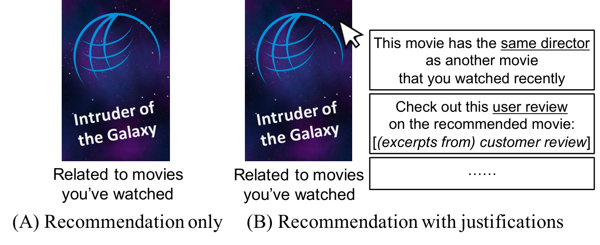
A product attribute, appropriately chosen in light of user preferences, naturally lends itself to an intuitive and concise justification. For instance, when the director James Cameron is chosen for a movie recommendation, this translates to the justification that “We recommend this movie directed by James Cameron, who made movies that are similar to other movies you watched.” When the user watched some of James Cameron’s movies, we can further enrich this justification with that information. Similarly, when a review gets selected, this translates to the justification like “Check out this user review, which closely reflects your preference, and explains why you should consider buying this item.” Figure 3 illustrates how such justifications enrich a movie recommendation, making the recommendation more persuasive. As in these examples, the final justifications can be generated based on custom rules that consider the attribute type and previous user actions. Note that, since our justifications are based on the product graph, the diversity of justifications increases as we add more product data to it, without needing to make changes to the framework.
II-C Quantifying the Quality of Justifications
To select good justifications tailored to the user and the recommendation, we need to be able to measure the goodness of product attributes. Towards this goal, we design justification scores, such that higher scores indicate better justifications in consideration of the product graph , products , and the recommended item . We quantify the justification score by considering two aspects, namely, relevance and diversity.
II-C1 Relevance Score
Intuitively, a good justification should be highly relevant to the recommended product . To measure the relevance of a product attribute, we consider how probable attribute is given the recommended product , that is,
| (1) |
where and are random variables denoting a recommended product, and an attribute of the recommended product, respectively. Consider a random variable , which denotes the product that matches the preference of user . Given products in , applying the sum rule of probability, the likelihood (1) can be expressed as:
| (2) |
Among the terms in (2), we know the user’s preferences on the products in , and have no information for other products. So, we assume that the products to which user gave no feedback are equally likely given the recommended item. Specifically, we assume that for all and any attribute . In other words, in measuring the relevance score, our focus is on the sum of likelihood terms of products in :
| (3) |
Symbol Definition Set of products Product recommended to user Set of products to which user gave positive feedback -th product in (i.e., ) Product attribute entity Set of all attribute entities Attribute entities of product Set of selected attribute entities Relative weight of in comparison to Non-negative weights for the justification diversity Budget (maximum number of justifications to select)
We observe that, by the product rule of probability, the following holds for each of the terms in (3):
| (4) |
where we have omitted random variables to simplify notations. In (4), the first term denotes the likelihood of attribute given product and recommended item , which closely matches our goal of finding a justification relevant to both the recommendation and the user’s preference. The second term represents how probable product is, given recommendation . This term measures the relevance of feedback with respect to , which enables considering the fact that some of the products in may not be relevant to the current recommendation. In other words, acts as a weight for the attribute relevance term.
Let denote the relevance score of attribute as a justification of the recommendation , which we define to be
| (5) |
Modeling Attribute and Feedback Relevance. We model the two relevance terms in (4) in terms of the product graph , as it provides rich information on how products and attributes are related to each other. Specifically, we consider a random walk using personalized PageRank (PPR) [14] over , and model the attribute relevance, , by the proximity of with respect to and in terms of PPR on . Intuitively, given a random walker who travels over and returns to and with a fixed probability, an attribute which gets visited more times than others is deemed more likely than other attributes, in terms of given and . We use the following notation
| (6) |
to denote the PPR score of attribute with respect to and , in which and are given the probability mass of and in the personalization vector, respectively, and controls the relative importance of in comparison to .
Note that PPR scores are computed for all nodes in , while we are concerned about the attributes of the recommended item. So we normalize PPR scores such that the scores of recommended item’s attributes sum to one, denoting the normalized score by nPPR. Then, is computed as
| (7) |
Similarly, we model the feedback relevance, , using PPR with respect to over , this time normalizing PPR scores over products in . Thus, is compute as
| (8) |
By (5), and our choice given by (7) and (8) to use nPPR on to model the relevance terms, we define as follows:
| (9) |
Finally, based on the above definition of attribute relevance (9), we define the relevance score of a set of attributes with respect to recommended product to be:
| (10) |
We show in Sections III and IV that our proposed approach yields more accurate relevance scores, which agree with our intuition, than other choices to model the attribute relevance.
II-C2 Diversity Score
To provide informative and engaging justifications to the user, we want the justifications to consist of diverse product attributes. For example, users would find it more interesting to see a combination of relevant reviews, product features, and purchasing history than seeing only reviews. Diversity has multiple aspects to it, and some aspects may be application dependent. Below we introduce two diversity aspects. Note that our method can easily be extended to incorporate different aspects of justification diversity.
We first consider the diversity in terms of attribute types. Let denote the type of attribute . We capture this diversity using the number of attribute types covered by the selected attributes :
| (11) |
Secondly, for textual product data such as customer reviews, we may consider the diversity of their topics and sentiments, which can be extracted by existing methods, e.g., by applying the latent Dirichlet allocation to product reviews with a decision threshold. Let denote the set of such topics of the textual data, and be the set of topics attribute represents. We capture this second diversity aspect using the number of topics attributes represent, defined by:
| (12) |
II-C3 Justification Score
Our goal is multi-objective as we aim to produce justifications with high relevance and diversity. We cast this into a single-objective optimization problem using a weighted sum scalarization. Since relevance and diversity terms can have different magnitude, we adopt the normalization scheme given in [15] such that each term is to be bounded between 0 and 1. For example, we define the first diversity term to be:
| (13) |
where and , with denoting the maximum number of attributes to be selected. Note that . In the event that and are equivalent, we define .
Applying the same normalization, we define the normalized relevance score and the topical diversity term as follows:
| (14) | ||||
| (15) |
where are defined in the same way as in the first term, using and instead of . In sum, given a recommended item , we define the justification score of a set of attributes as:
| (16) |
where and are non-negative weights for diversity terms.
II-D Justification Discovery
Based on the above definition of relevance, diversity, and justification scores, we formally define the justification discovery problem as follows.
Due to the combinatorial nature of this optimization problem, solving it exactly is computationally intractable. Instead, we show that the objective (17) is submodular, which allows us to efficiently obtain near-optimal justifications.
Theorem 1.
The justification score given by (16) is a non-negative, monotone, submodular function.
Proof.
(a) is non-negative since it is a weighted sum of three non-negative scores with non-negative weights.
(b) A set function is monotone if for every , we have that . Given that
is monotone as it is a non-negative weighted sum of these monotone scores.
(c) Given a set function of attributes , and attribute , let be the marginal gain of adding to . Then is submodular if for every with and every , it holds that .
As every results in the same marginal gain to both and , .
Let . The topics covered by can be classified into three cases. The first case is the set of topics that belong to . Since , ; thus, these topics make no additional contributions to both and . The second case is the set of topics that do not belong to , but belong to . Since these topics already belong to , they make positive contributions to , while making no contributions to . The third case is the set of topics that do not belong to both and . In this case, the topics in make equal contributions to and . Thus, in all cases, . The same argument applies to show that .
Therefore, since three functions , and are all submodular, the justification score , which is a weighted sum of these submodular functions with non-negative weights, is also submodular. ∎
Theorem 2.
1 admits a -approximation.
Proof.
Maximizing a non-negative, monotone, submodular function subject to a cardinality constraint admits a approximation under a greedy approach in which the item with the largest marginal gain is selected at each step [16]. This theorem follows since our maximization objective is non-negative, monotone, and submodular by Theorem 1. ∎
J-Recs algorithm. Theorem 2 leads to the J-Recs algorithm in Algorithm 1, which finds a -approximation of the optimal justifications. In Algorithm 1, we first compute the relevance score of all attributes based on (9). Then, we repeatedly find the product attribute from with the greatest marginal gain, where is the attributes of product , and add it to until we exhaust the given budget .
return
Theorem 3.
Algorithm 1 runs in time with processors, taking steps in total, assuming that , where with and denoting the number of attribute types and topics, respectively.
Proof.
Computing the relevance score in (9) for all attributes involves computing the scores with respect to personalization vectors. Using a power iteration with sparse matrix multiplications, can be computed in time. Since computations are independent of each other, they can be completed in time using processors.
Computing corresponds to the maximum coverage problem. As this is NP-hard, we use a greedy approximation algorithm [17], which takes time. Other terms for score normalization (e.g., ) can also be computed in time. Then we select up to justifications: Selecting one justification requires evaluating the marginal gain for all . As evaluating the marginal gain with respect to each term in (16) takes , greedy selection takes steps in total. Given that and assuming , which is true in most cases, the running time for the greedy selection is . ∎
III Evaluation Using Axioms
In this section, we evaluate different approaches to measure attribute relevance, using what we call axioms, which are a set of product graphs with an intuitive expected outcome. After describing axioms, we introduce other approaches to compute attribute relevance, and discuss how well axioms are satisfied by different approaches. Experimental settings used for this evaluation are given in Section -A.
1. Proximity 2. Feedback Relevance 3. Popularity 4. Edge Weight Awareness 5. Product Data Scarcity 6. Community Awareness 7. Long Path Connectivity J-Recs ExpLOD [18] MP-AND [19] MP-OR [19] [20] [20] [20] [20] MP-AND w/ HAR [21] authority score MP-OR
III-A Axioms
An axiom is a small product graph with expected relevance scores (9) for some product attributes. We use the axioms shown in Figure 4 to evaluate different methods for measuring attribute relevance. In Figure 4, squares denote product attributes, and circles denote products, where is the recommended product, is the product with positive user feedback, and is a product the user had no interaction with.
1. Proximity. Attributes that are closer to products and should receive a higher relevance score. Given that is directly connected to and (i.e., is a shared attribute of and ), while other attributes are three hops away from either or , we expect .
2. Feedback Relevance. Attributes that receive more support from the products in should receive a higher relevance score. While both and are directly connected to , is covered by a greater number of products in . Thus, we expect .
3. Popularity. More widely used attributes should receive a higher relevance score (e.g., consider explaining a movie recommendation with a popular actor vs. an actor who appeared only in that movie). Thus, we require that .
4. Edge Weight Awareness. Attributes that are connected via edges of higher weight should receive a higher relevance score, as edge weight indicates the importance of each connection in the product graph. Thus, we expect . Note that satisfying this axiom is important to reflect the relative importance among different attribute types. For instance, while country attributes would be one of the most popular ones in the movie product graph, it may not be a very interesting justification to the user. Based on this prior knowledge, we can downplay the country type if our method satisfies this axiom.
5. Product Data Scarcity. Attributes of the product that contain scarcer information should receive a higher relevance score. This axiom consists of two product graphs, in which each attribute is directly connected to and . While each graph contains only one product in , the positive feedback expressed by is attributed to multiple attributes in the larger graph, leading to each one of them being a weaker evidence of user’s preference than the other product’s unique attribute. Thus, we expect for .
6. Community Awareness. When the recommended item belongs to one community (e.g., a group of shoes), it is desirable to put more weight on attributes belonging to the same community than on others (e.g., a group of electronic devices), as similar products tend to share more attributes (e.g., product details, keywords) with each other than with different products. In this axiom, there are two small communities of products and attributes, where and act as a bridge between communities. Also, each community has only one product with positive feedback. Therefore, we expect .
7. Long Path Connectivity. Even when attributes are not directly connected to and , attributes more strongly connected to and should receive a higher relevance score. Here, is more strongly linked to via and than , which is linked to only via . Thus, we expect .
III-B Baselines
Below we use the same notation as in (6) to specify the query nodes. Table I provides the definition of symbols.
III-B1 Relevance Models
We consider three approaches that measure the relevance of attribute , given recommendation and products .
ExpLOD [18] assigns a high score to those attributes that are highly connected to the products in , using the following formula:
| (18) |
where is the number of edges between product attribute and the products in , is the number of edges between and , and is the reciprocal of the number of products that are described by attribute .
Meeting Probability (MP) [19] assigns a high relevance score to an attribute that is close to the recommended item and products . MP has been successfully used in identifying nodes that have strong connections to the query nodes. We consider the following two MP scores.
| (19) | ||||
| (20) |
BASSET (BA) [20] aims to identify a small number of good gateway nodes between a source node and a target node in the given graph. Let denote the PPR score from source to target , after setting the nodes denoted by as sinks (i.e., nodes with no outgoing edges). We also consider a related model, , in which we delete the nodes denoted by , instead of making them sinks. Note that, in out setting, given a recommendation and a product , we can consider two directions of and . For instance, BA score of attribute between source and target using is defined as:
| (21) |
Three other options, , , and are defined analogously.
III-B2 Proximity Measure
A proximity measure provides a way to compute node proximity with respect to a query node. We consider two important proximity measures.
PPR (Personalized PageRank) [14] measures node-to-node proximity by the limiting probability distribution of a random walker biased towards a set of query nodes.
HAR [21] is a generalization of SALSA [22] to handle multi-relational data, which enables users to specify the relative importance of relations. HAR has been shown to outperform SALSA [22] and HITS [23] in identifying relevant results to the query input. HAR computes hub score and authority score with respect to a query entity. While we considered both scores as a proximity measure, due to space constraints, we report only the result obtained with authority score as hub score was mostly outperformed by authority score.
Among the relevance models introduced above, MP and BA internally use PPR. We evaluate variants of these baselines using HAR as their proximity measure (except for ExpLOD, which is not a random walk-based method).
III-C Results
Table II summarizes which axioms are satisfied by different approaches to measure attribute relevance. A checkmark indicates that the expected outcome of the axiom has been achieved by the corresponding method. J-Recs is the only one that satisfies all axioms. Other alternatives fail at least one of the axioms; among them, is the next best one, failing only (6) Community Awareness axiom. In Section IV, we show that J-Recs also leads to more accurate justifications than in experiments using real-world product graphs.
does not satisfy most of the axioms, mainly due to the fact that it can only consider direct edges between products and attributes, failing to propagate information over the graph.
In general, BASSET (BA) led to worse results than J-Recs and , failing (1) Popularity, (6) Community Awareness, and (7) Long Path Connectivity axioms in many cases, indicating that good gateway nodes may not serve well as a justification. Also, while achieved a reasonably good result (for instance, with MP-AND), relevance models could satisfy more axioms using as a proximity measure.
IV Evaluation Using Real-World Data
In this section, we address the following questions.
- Q1.
Justification Quality. How well does J-Recs justify recommendations?
- Q2.
Scalability. How does J-Recs scale up with the increase of the input size?
- Q3.
Relevance-Diversity Trade-Off. How does increasing the weight for diversity affect the relevance of justifications?
Experimental settings are given in Section -A.
Name Product # Products # Nodes # Edges movie-pg Movie 4,803 308,304 1,329,428 citation-pg Paper 11,941 111,007 724,962 citation-100m-pg Paper 2,094,396 7,426,773 100,000,000
IV-A Datasets
We construct product graphs from public datasets on movies and publications. Table III shows the statistics of our datasets.
movie-pg consists of movies and movie-related attributes, such as actors, directors, crews, casts, and movie keywords, extracted from the TMDb 5000 movie dataset11 1 https://www.kaggle.com/tmdb/tmdb-movie-metadata. We also added positive reviews to movie-pg, which gave 10/10 rating to the movies. Reviews were retrieved from the IMDb website22 2 https://www.imdb.com/, instead of TMDb, since more reviews were available on IMDb. We extracted keywords from each review, by filtering out those words whose tf-idf score is below a threshold, and connected them with the reviews.
citation-pg is a product graph of papers and related attributes, such as authors, citations, publication venues, and fields of study, constructed from the citation network dataset v12 [24]33 3 https://www.aminer.org/citation. In citation-pg, we included papers published at KDD, SIGMOD, and ICML, and their attributes, while excluding papers that were cited less than 5 times. We also created citation-100m-pg that contains edges for scalability evaluation, which is also constructed from the same citation network dataset, and includes all venues and papers.
IV-B Baselines
Among the baselines used in Section III, we use MP-AND and MP-OR [19], which satisfied most axioms among baselines, and [18], which is a representative non-random walk based method for justifying recommendations. Among them, we exclude BA and (which was used as a proximity measure) as they were mostly outperformed by other alternatives. We also include [25], which estimates attribute relevance by its PageRank score in the product graph.
IV-C Q1. Justification Quality
We evaluate the quality of justifications in two ways: automatic evaluation and qualitative analysis.
IV-C1 Automatic Evaluation
For an automatic and objective evaluation, we consider the task of user preference retrieval.
User Preference Retrieval. Among several attributes of the recommended product , we want those that reflect the user’s preference better than others to receive higher relevance scores and be used as a justification. In our two datasets, the review and the paper written by a user clearly reflect the user’s preference. Thus, among the reviews and papers associated with recommended product , it is desirable for the review and paper written by the user to get higher scores than others.
For movie-pg, we select a positive review written by the user who wrote at least 10 positive reviews. Note that the movies for which user wrote positive reviews correspond to . Similarly, for citation-pg, we select a reference written by the user who published at least 15 papers. In total, we randomly select 50 reviews and 50 citations.
Performance Evaluation. We evaluate preference retrieval results using the mean reciprocal rank (MRR). Let denote the chosen attributes of a specific type (e.g., reviews or cited papers), written by different users. Let refer to the product of -th attribute in (e.g., the product for which the -th review was written), and be the rank position of the -th attribute among the corresponding attributes of product , where ranks are determined by the estimated relevance score computed with respect to and the products that received positive feedback by user who created the -th attribute (e.g., movies that received positive reviews by user ). MRR is defined by
| (22) |
and higher values are better.
Results. Figure 1 shows the MMR on two datasets. J-Recs achieved the best MMR, which is up to 20.7% higher than the second best result achieved by MP-AND. While MP-OR outperformed MP-AND on citation-pg by a small margin, results show that MP-OR’s performance is more sensitive to the dataset than MP-AND. ’s performance is worse than J-Recs as it does not consider and in measuring attribute relevance. Since each review applies to only one product, ends up assigning identical scores to all reviews, making it inapplicable to be used to retrieve user preferences on movie-pg. On citation-pg, obtains even lower MMR than , which is due to the fact that computes relevance score based only on the direct connection between products and attributes, failing to propagate user preference over a graph.
Note that since we ignore the relevance of other reviews and citations, which is unknown to us, these results are a lower bound of the true MMR. As MMR considers the rank of the first relevant entity, the true MMR would be higher than the current result if there is another relevant attribute, ranked higher than the user’s review and paper.
J-Recs () J-Recs () MP-AND [19] Positive tensor factorization Tensor decompositions and applications Tensor decompositions and applications Tensor decompositions and applications Positive tensor factorization Distributed optimization and statistical learning via the alternating direction method of multipliers Marble: high-throughput phenotyping from electronic health records via sparse nonnegative tensor factorization Marble: high-throughput phenotyping from electronic health records via sparse nonnegative tensor factorization Positive tensor factorization On tensors, sparsity, and nonnegative factorizations Limestone: high-throughput candidate phenotype generation via tensor factorization Scalable tensor factorizations for incomplete data Limestone: high-throughput candidate phenotype generation via tensor factorization On tensors, sparsity, and nonnegative factorizations Learning with tensors: a framework based on convex optimization and spectral regularization Distributed optimization and statistical learning via the alternating direction method of multipliers Scalable tensor factorizations for incomplete data Marble: high-throughput phenotyping from electronic health records via sparse nonnegative tensor factorization Scalable tensor factorizations for incomplete data Distributed optimization and statistical learning via the alternating direction method of multipliers A block coordinate descent method for regularized multiconvex optimization with applications to nonnegative tensor factorization and completion Tensor completion for estimating missing values in visual data Tensor completion for estimating missing values in visual data On tensors, sparsity, and nonnegative factorizations Network discovery via constrained tensor analysis of fMRI data Network discovery via constrained tensor analysis of fMRI data Tensor completion for estimating missing values in visual data Learning with tensors: a framework based on convex optimization and spectral regularization Next-generation phenotyping of electronic health records Network discovery via constrained tensor analysis of fMRI data Next-generation phenotyping of electronic health records Learning with tensors: a framework based on convex optimization and spectral regularization Limestone: high-throughput candidate phenotype generation via tensor factorization Square deal: lower bounds and improved relaxations for tensor recovery Square deal: lower bounds and improved relaxations for tensor recovery Next-generation phenotyping of electronic health records FlexiFaCT: scalable flexible factorization of coupled tensors on Hadoop FlexiFaCT: scalable flexible factorization of coupled tensors on Hadoop Square deal: lower bounds and improved relaxations for tensor recovery All-at-once optimization for coupled matrix and tensor factorizations All-at-once optimization for coupled matrix and tensor factorizations Convex tensor decomposition via structured Schatten norm regularization A block coordinate descent method for regularized multiconvex optimization with applications to nonnegative tensor factorization and completion Convex tensor decomposition via structured Schatten norm regularization A new convex relaxation for tensor completion
IV-C2 Qualitative Analysis
We present two case studies where we compare the results obtained with J-Recs and MP-AND on citation-pg. To see how the parameter in (9) affects J-Recs, we report two results for J-Recs using and .
Case 1. J-Recs and MP-AND are given the paper entitled “Rubik: Knowledge Guided Tensor Factorization and Completion for Health Data Analytics” [26] as a recommended item , and the set with ten papers on matrix and tensor factorizations. Table IV shows top-15 papers cited by the recommended paper, ordered by the relevance computed with J-Recs (9) and MP-AND (19). The papers in blue font deal with electronic health record (EHR) analysis, and those highlighted in cyan background color are two highly relevant papers that employ tensor factorization for EHR analysis. Among the citations, these highlighted papers are particularly relevant justifications, since they cut across two topics central to the recommended paper and the papers in , namely, EHR analysis and tensor factorization. In Table IV, these two highly relevant papers belong to the top-5 citations in both results of J-Recs, while they are ranked at 6th and 11th places in the result of MP-AND. Further, since EHR analysis is a major topic of the recommended paper, with , J-Recs gives more weight to EHR analysis than with , which boosts the ranking of the papers on EHR analysis.
Case 2. J-Recs and MP-AND are given the paper entitled “Towards Parameter-Free Data Mining” [27] as a recommended item , and the set with ten papers on time series analysis. Table V shows top-15 papers cited by the recommended paper, ordered by the relevance computed with J-Recs (9) and MP-AND (19). The citations in blue font are the papers relevant to the MDL principle. Among the cited publications, those on MDL are highly relevant justifications as MDL principle is central to the main idea of the recommended paper. At the same time, since contains papers on time series analysis, references on time series are relevant. In Table V, J-Recs retrieves four papers on MDL (ranked at 2nd, 7th, 11th, and 13th places with ), and eleven papers on time series. On the other hand, MP-AND retrieves only two papers on MDL (ranked at 7th and 14th places). Also, in this case, increasing to led to a more drastic change than in the previous case, boosting the ranking of the papers on MDL.
Overall, in these case studies, J-Recs produces qualitatively better results than MP-AND, which are more balanced in terms of the relevance to the recommendation, user preferences, and the diversity of paper topics.
J-Recs () J-Recs () MP-AND [19] On the need for time series data mining benchmarks: a survey and empirical demonstration On the need for time series data mining benchmarks: a survey and empirical demonstration On the need for time series data mining benchmarks: a survey and empirical demonstration Making time-series classification more accurate using learned constraints An introduction to Kolmogorov complexity and its applications Clustering of time series subsequences is meaningless: implications for previous and future research Distance measures for effective clustering of ARIMA time-series Making time-series classification more accurate using learned constraints A symbolic representation of time series, with implications for streaming algorithms Deformable Markov model templates for time-series pattern matching Distance measures for effective clustering of ARIMA time-series Making time-series classification more accurate using learned constraints TSA-tree: a wavelet-based approach to improve the efficiency of multi-level surprise and trend queries on time-series data Deformable Markov model templates for time-series pattern matching Distance measures for effective clustering of ARIMA time-series Mining the stock market: which measure is best? TSA-tree: a wavelet-based approach to improve the efficiency of multi-level surprise and trend queries on time-series data Mining the stock market: which measure is best? Supporting content-based searches on time series via approximation Modeling by shortest data description Modeling by shortest data description Clustering of time series subsequences is meaningless: implications for previous and future research Mining the stock market: which measure is best? Deformable Markov model templates for time-series pattern matching An introduction to Kolmogorov complexity and its applications A symbolic representation of time series, with implications for streaming algorithms Indexing multi-dimensional time-series with support for multiple distance measures A symbolic representation of time series, with implications for streaming algorithms Clustering of time series subsequences is meaningless: implications for previous and future research FastMap: a fast algorithm for indexing, data-mining and visualization of traditional and multimedia datasets Indexing multi-dimensional time-series with support for multiple distance measures Inferring decision trees using the minimum description length principle TSA-tree: a wavelet-based approach to improve the efficiency of multi-level surprise and trend queries on time-series data Modeling by shortest data description Supporting content-based searches on time series via approximation Online novelty detection on temporal sequences Inferring decision trees using the minimum description length principle The similarity metric Supporting content-based searches on time series via approximation The similarity metric Indexing multi-dimensional time-series with support for multiple distance measures Inferring decision trees using the minimum description length principle Online novelty detection on temporal sequences Online novelty detection on temporal sequences Graph-based anomaly detection
IV-D Q2. Scalability
To evaluate the scalability of J-Recs, we created increasingly larger subgraphs of citation-100m-pg, with each subgraph being larger than the previous one. Figure 5 reports the running time of J-Recs on these product graphs of varying sizes, where the running time was averaged over three simulated users with at least ten products in his . The results show that J-Recs achieves near-linear scalability, successfully scaling up to the largest graph with edges.
IV-E Q3. Relevance-Diversity Trade-Off
We measure how varying , the weight for the attribute type diversity, affects the relevance score and the diversity score of the selected attributes . Specifically, we randomly selected 50 users from movie-pg, who rated at least 10 movies, and generated 30 justifications varying from 0 to 0.6. In Figure 6, we report relevance and diversity scores averaged over all users. Figure 6 shows that while there is a trade-off between relevance and diversity, it is possible to attain high relevance and diversity. As is increased from 0 to 0.3, increases by 148%, while decreases by 7%. Results indicate that setting to an appropriate value can be beneficial in providing diverse and relevant justifications to the users.
V Related Work
Explainable Recommendation. Methods for explainable recommendation can be grouped into embedded and post-hoc approaches. Embedded approaches [28, 29, 30, 31, 32] aim to develop interpretable models, such that explanations for the model decision can be naturally provided. While embedded methods have high model explainability, different explanation techniques need to be developed for different types of recommendation methods. Our framework is model-agnostic and can be applied to different recommenders flexibly. We refer the reader to [11] for an in-depth review of embedded methods.
In post-hoc approaches, explanations and recommendations are generated from separate models. Post-hoc explanations are often item-based (e.g., “Customers who bought this item also bought” [8]), neighbor-based (e.g., “Your neighbors’ rating for this item is” [6]), and content-based (e.g., keywords [9], features [33], tags [10], or reviews [34, 35]). Since these methods typically select an explanation based on one of manually defined templates or generate explanations using one type of data, the diversity of their explanations are limited by the form of such templates or the type of input data. On the other hand, J-Recs is a unified framework that can work with multiple types of data, and its diversity increases as we provide more data to the framework. ExpLOD [18] provides more diverse explanations than earlier methods by using linked open data cloud in a graph-based framework. However, ExpLOD and others such as [10] produce justifications only using the items in the user profile, ignoring other items and their attributes relevant to the recommendation and the user profile. By using random walk-based node proximity, J-Recs utilizes both the user profile and other data relevant to it.
Node Importance. PageRank (PR) [25] measures node importance by considering the limiting probability of a random surfer that travels over a graph following any out-going edge with uniform probability. The original PR does not depend on the query, and personalized PR (PPR) [14] followed PR to estimate query-dependent node importance. Random walk with restart (RWR) [36, 37] can be seen as a special case of PPR that considers one query node. HITS [23] first retrieves a focused subgraph with respect to the search query, and computes hub and authority scores for each node in the focused subgraph. SALSA [22] can be considered as an improvement of HITS, which also computes hub and authority scores like HITS, while less susceptible to the tightly knit community (TKC) effect than HITS. HAR [21] is a generalization of SALSA that deals with multi-relation data, and computes hub and authority scores for objects and relevance scores for relations, with respect to a query input. GENI [38] and MultiImport [39] are semi-supervised techniques to estimate node importance by considering both the graph structure and real-world signals of node popularity. Among the above methods, query-sensitive ones can be used to measure node-to-node proximity, which have also been used to identify a subset of nodes or a subgraph, which have strong connections to the query nodes [40, 19] and are important in connecting source and target nodes [20, 41]. In this work, we consider the effectiveness of these approaches for the task of recommendation justification, and use the most effective ones to define the relevance score, which best satisfy the axioms of good justifications.
VI Conclusion
In this paper, we present a graph-based formulation of the problem of recommendation justification, and develop J-Recs, a unified model-agnostic framework which can produce concise, diverse, and personalized justifications in a principled manner, based on various types of product and user data. We show the effectiveness and efficiency of J-Recs in an evaluation using axioms and real-world data. In this work, we propose preference retrieval as one way of evaluating the justification quality. Developing additional automatic and objective evaluation metrics that can measure the quality of justifications from different perspectives will also be an important direction for future research on explainable recommendations.
References
- [1] Y. Koren, R. M. Bell, and C. Volinsky, “Matrix factorization techniques for recommender systems,” IEEE Computer, vol. 42, no. 8, 2009.
- [2] S. Zhang, W. Wang, J. Ford, and F. Makedon, “Learning from incomplete ratings using non-negative matrix factorization,” in SDM, 2006.
- [3] H. Wang, N. Wang, and D. Yeung, “Collaborative deep learning for recommender systems,” in KDD, 2015, pp. 1235–1244.
- [4] W. Fan, Y. Ma, Q. Li, Y. He, Y. E. Zhao, J. Tang, and D. Yin, “Graph neural networks for social recommendation,” in WWW, 2019.
- [5] O. Biran and C. Cotton, “Explanation and justification in machine learning: A survey,” in IJCAI-17 workshop on explainable AI (XAI), vol. 8, no. 1, 2017.
- [6] J. L. Herlocker, J. A. Konstan, and J. Riedl, “Explaining collaborative filtering recommendations,” in Proceedings of the 2000 ACM conference on Computer supported cooperative work, 2000, pp. 241–250.
- [7] N. Tintarev and J. Masthoff, “A survey of explanations in recommender systems,” in ICDE, 2007, pp. 801–810.
- [8] ——, “Explaining recommendations: Design and evaluation,” in Recommender Systems Handbook, 2015, pp. 353–382.
- [9] M. Bilgic and R. J. Mooney, “Explaining recommendations: Satisfaction vs. promotion,” in Beyond Personalization Workshop, IUI, vol. 5, 2005.
- [10] J. Vig, S. Sen, and J. Riedl, “Tagsplanations: explaining recommendations using tags,” in IUI, 2009, pp. 47–56.
- [11] Y. Zhang and X. Chen, “Explainable recommendation: A survey and new perspectives,” Found. Trends Inf. Retr., vol. 14, no. 1, 2020.
- [12] L. Dong, S. Huang, F. Wei, M. Lapata, M. Zhou, and K. Xu, “Learning to generate product reviews from attributes,” in EACL, 2017.
- [13] J. Ni, J. Li, and J. J. McAuley, “Justifying recommendations using distantly-labeled reviews and fine-grained aspects,” in EMNLP-IJCNLP, 2019, pp. 188–197.
- [14] T. H. Haveliwala, “Topic-sensitive pagerank,” in WWW, 2002.
- [15] O. Grodzevich and O. Romanko, “Normalization and other topics in multi-objective optimization,” 2006.
- [16] G. L. Nemhauser and L. A. Wolsey, “Best algorithms for approximating the maximum of a submodular set function,” Math. Oper. Res., vol. 3, no. 3, pp. 177–188, 1978.
- [17] J. Kleinberg and E. Tardos, Algorithm design. Pearson Education, 2006.
- [18] C. Musto, F. Narducci, P. Lops, M. de Gemmis, and G. Semeraro, “Explod: A framework for explaining recommendations based on the linked open data cloud,” in RecSys, 2016, pp. 151–154.
- [19] H. Tong and C. Faloutsos, “Center-piece subgraphs: problem definition and fast solutions,” in KDD, 2006, pp. 404–413.
- [20] H. Tong, S. Papadimitriou, C. Faloutsos, P. S. Yu, and T. Eliassi-Rad, “BASSET: scalable gateway finder in large graphs,” in PAKDD, 2010.
- [21] X. Li, M. K. Ng, and Y. Ye, “HAR: hub, authority and relevance scores in multi-relational data for query search,” in SDM, 2012, pp. 141–152.
- [22] R. Lempel and S. Moran, “SALSA: the stochastic approach for link-structure analysis,” ACM Trans. Inf. Syst., vol. 19, no. 2, 2001.
- [23] J. M. Kleinberg, “Authoritative sources in a hyperlinked environment,” J. ACM, vol. 46, no. 5, pp. 604–632, 1999.
- [24] J. Tang, J. Zhang, L. Yao, J. Li, L. Zhang, and Z. Su, “Arnetminer: extraction and mining of academic social networks,” in KDD, 2008.
- [25] L. Page, S. Brin, R. Motwani, and T. Winograd, “The pagerank citation ranking: Bringing order to the web.” Stanford InfoLab, Tech. Rep., 1999.
- [26] Y. Wang, R. Chen, J. Ghosh, J. C. Denny, A. N. Kho, Y. Chen, B. A. Malin, and J. Sun, “Rubik: Knowledge guided tensor factorization and completion for health data analytics,” in KDD, 2015, pp. 1265–1274.
- [27] E. J. Keogh, S. Lonardi, and C. A. Ratanamahatana, “Towards parameter-free data mining,” in KDD, 2004, pp. 206–215.
- [28] X. Wang, X. He, F. Feng, L. Nie, and T. Chua, “TEM: tree-enhanced embedding model for explainable recommendation,” in WWW, 2018.
- [29] J. Chen, H. Zhang, X. He, L. Nie, W. Liu, and T. Chua, “Attentive collaborative filtering: Multimedia recommendation with item- and component-level attention,” in SIGIR, 2017, pp. 335–344.
- [30] Q. Diao, M. Qiu, C. Wu, A. J. Smola, J. Jiang, and C. Wang, “Jointly modeling aspects, ratings and sentiments for movie recommendation (JMARS),” in KDD, 2014, pp. 193–202.
- [31] X. Chen, H. Chen, H. Xu, Y. Zhang, Y. Cao, Z. Qin, and H. Zha, “Personalized fashion recommendation with visual explanations based on multimodal attention network: Towards visually explainable recommendation,” in SIGIR, 2019, pp. 765–774.
- [32] Y. Zhang, G. Lai, M. Zhang, Y. Zhang, Y. Liu, and S. Ma, “Explicit factor models for explainable recommendation based on phrase-level sentiment analysis,” in SIGIR, 2014, pp. 83–92.
- [33] N. Tintarev, “Explanations of recommendations,” in Proceedings of the 2007 ACM Conference on Recommender Systems, RecSys 2007, Minneapolis, MN, USA, October 19-20, 2007, 2007, pp. 203–206.
- [34] T. Donkers, B. Loepp, and J. Ziegler, “Explaining recommendations by means of user reviews,” in Joint Proceedings of the ACM IUI 2018 Workshops co-located with the 23rd ACM Conference on Intelligent User Interfaces (ACM IUI 2018), Tokyo, Japan, March 11, 2018, 2018.
- [35] X. Wang, Y. Chen, J. Yang, L. Wu, Z. Wu, and X. Xie, “A reinforcement learning framework for explainable recommendation,” in ICDM, 2018.
- [36] H. Tong, C. Faloutsos, and J. Pan, “Random walk with restart: fast solutions and applications,” Knowl. Inf. Syst., vol. 14, no. 3, 2008.
- [37] J. Jung, N. Park, L. Sael, and U. Kang, “Bepi: Fast and memory-efficient method for billion-scale random walk with restart,” in SIGMOD, 2017.
- [38] N. Park, A. Kan, X. L. Dong, T. Zhao, and C. Faloutsos, “Estimating node importance in knowledge graphs using graph neural networks,” in KDD, 2019, pp. 596–606.
- [39] ——, “Multiimport: Inferring node importance in a knowledge graph from multiple input signals,” in KDD, 2020, pp. 503–512.
- [40] C. Faloutsos, K. S. McCurley, and A. Tomkins, “Fast discovery of connection subgraphs,” in KDD, 2004, pp. 118–127.
- [41] H. Tong, S. Papadimitriou, C. Faloutsos, P. S. Yu, and T. Eliassi-Rad, “Gateway finder in large graphs: problem definitions and fast solutions,” Inf. Retr., vol. 15, no. 3-4, pp. 391–411, 2012.
-A Experimental Settings
Machine. We ran experiments on a machine with 32 Intel Xeon CPU E7-8837 cores at 2.67GHz, and 1 TB of memory.