跳到论文正文
W Papers独立论文阅读器 arXiv:2011.05909 论文正文 计算阅读时间 · 0%
引用这篇论文根据当前论文元数据生成,正式投稿前建议核对。


License: CC BY 4.0
arXiv:2011.05909v1 [math.DS] 11 Nov 2020

Directed harmonic currents near
non-hyperbolic linearized singularities

Zhangchi Chen
August 11, 2026
Abstract

Let (𝔻2,ℱ,{0})(\mathbb{D}^{2},\mathscr{F},\{0\}) be a singular holomorphic foliation on the unit bidisc 𝔻2\mathbb{D}^{2} defined by the linear vector field

z​∂∂z+λ​w​∂∂w,z\,\frac{\partial}{\partial z}+\lambda\,w\,\frac{\partial}{\partial w},

where λ∈ℂ∗\lambda\in\mathbb{C}^{*}. Such a foliation has a non-degenerate linearized singularity at 00. Let TT be a harmonic current directed by ℱ\mathscr{F} which does not give mass to any of the two separatrices (z=0)(z=0) and (w=0)(w=0) and whose the trivial extension T~\tilde{T} across 00 is d​dcdd^{c}-closed. The Lelong number of TT at 00 describes the mass distribution on the foliated space. In 2014 Nguyen proved that when λ∉ℝ\lambda\notin\mathbb{R}, i.e. 00 is a hyperbolic singularity, the Lelong number at 00 vanishes. For the non-hyperbolic case λ∈ℝ∗\lambda\in\mathbb{R}^{*} the article proves the following results. The Lelong number at 00:

1) is strictly positive if λ>0\lambda>0;

2) vanishes if λ∈ℚ<0\lambda\in\mathbb{Q}_{<0};

3) vanishes if λ<0\lambda<0 and TT is invariant under the action of some cofinite subgroup of the monodromy group.

Keywords:  Holomorphic foliation, Harmonic current, Non-hyperbolic linearized singularity, Lelong number.

1 Introduction

The dynamical properties of holomorphic foliations have drawn great attention recently [40]. Let us see one of the recent interesting results.

Theorem 1.1 (Dinh-Nguyên-Sibony [20]).

Let ℱ\mathscr{F} be a holomorphic foliation with only hyperbolic singularities in a compact Kähler surface (X,ω)(X,\omega). Assume that ℱ\mathscr{F} admits no directed positive closed current. Then there exists a unique positive d​dcdd^{c}-closed current TT of mass 11 directed by ℱ\mathscr{F}.

The first version was stated for X=ℙ2X=\mathbb{P}^{2} and proved by Fornæss-Sibony [28]. Later Dinh-Sibony proved unique ergodicity for foliations in ℙ2\mathbb{P}^{2} with an invariant curve [23]. So one may expect to describe recurrence properties of leaves by studying the density distribution of directed harmonic currents. One has the following the result about leaves.

Theorem 1.2 (Fornæss-Sibony [28]).

Let (X,ℱ,E)(X,\mathscr{F},E) be a hyperbolic foliation on a compact complex surface XX with singular set EE. Assume that

  1. 1.

    there is no invariant analytic curve;

  2. 2.

    all the singularities are hyperbolic;

  3. 3.

    there is no non-constant holomorphic map ℂ→X\mathbb{C}\rightarrow X such that out of EE the image of ℂ\mathbb{C} is locally contained in a leaf.

Then every harmonic current TT directed by ℱ\mathscr{F} gives no mass to each single leaf.

A practical way to measure the density of harmonic currents is to use the notion of Lelong number introduced by Skoda [49]. Indeed Theorem 1.2 above is equivalent to the statement that the Lelong number of TT vanishes everywhere outside EE. Another result holds near hyperbolic singularities.

Theorem 1.3 (Nguyên [34]).

Let (𝔻2,ℱ,{0})(\mathbb{D}^{2},\mathscr{F},\{0\}) be a holomorphic foliation on the unit bidisc 𝔻2\mathbb{D}^{2} defined by the linear vector field Z⁡(z,w)=z​∂∂z+λ​w​∂∂w,Z(z,w)=z\,\frac{\partial}{\partial z}+\lambda\,w\,\frac{\partial}{\partial w}, where λ∈ℂ\ℝ\lambda\in\mathbb{C}\backslash\mathbb{R}, that is to say, 00 is a hyperbolic singularity. Let TT be a harmonic current directed by ℱ\mathscr{F} which does not give mass to any of the two separatrices (z=0)(z=0) and (w=0)(w=0). Then the Lelong number of TT at 00 vanishes.

Nguyên proved that the Lelong number of any directed harmonic current which gives no mass to invariant hyperplanes, vanishes near weakly hyperbolic singularities in ℂn\mathbb{C}^{n} [40]. This result is optimal, see [25]. The mass-distribution problem would be completed once the behaviour of harmonic currents near non-hyperbolic and near degenerate singularities would be understood.

The present paper answers (partly) the problem in the non-hyperbolic linearizable singularity case.

Theorem 1.4.

Let (𝔻2,ℱ,{0})(\mathbb{D}^{2},\mathscr{F},\{0\}) be a holomorphic foliation on the unit bidisc 𝔻2\mathbb{D}^{2} defined by the linear vector field Z⁡(z,w)=z​∂∂z+λ​w​∂∂wZ(z,w)=z\,\frac{\partial}{\partial z}+\lambda\,w\,\frac{\partial}{\partial w}, where λ∈ℝ∗\lambda\in\mathbb{R}^{*}. Let ℱ\mathscr{F} be a harmonic current directed by ℱ\mathscr{F} which does not give mass to any of the two separatrices (z=0)(z=0) and (w=0)(w=0). Then the Lelong number of TT at 00

  • •

    is strictly positive if λ>0\lambda>0,

  • •

    vanishes if λ∈ℚ<0\lambda\in\mathbb{Q}_{<0}.

For the concerned foliation (𝔻2,ℱ,{0})(\mathbb{D}^{2},\mathscr{F},\{0\}), a local leaf PαP_{\alpha}, with α∈ℂ∗\alpha\in\mathbb{C}^{*}, can be parametrized by (z,w)=(e−v+i​u,α​e−λ​v+i​λ​u)(z,w)=(e^{-v+iu},\alpha\,e^{-\lambda v+i\lambda u}). The monodromy group around the singularity is generated by (z,w)↦(z,e2​π​i​λ​w)(z,w)\mapsto(z,e^{2\pi i\lambda}w). It is a cyclic group of finite order when λ∈ℚ∗\lambda\in\mathbb{Q}^{*}, of infinite order when λ∉ℚ\lambda\notin\mathbb{Q}.

It is now ready to introduce the notion of periodic current, an essential tool of this paper. A directed harmonic current TT is called periodic if it is invariant under some cofinite subgroup of the monodromy group, i.e. under the action of (z,w)↦(z,e2​k​π​i​λ​w)(z,w)\mapsto(z,e^{2k\pi i\lambda}w) for some k∈ℤ>0k\in\mathbb{Z}_{>0}. Observe that if λ∈ℚ∗\lambda\in\mathbb{Q}^{*} then any directed harmonic current is periodic. But when λ∉ℚ∗\lambda\notin\mathbb{Q}^{*}, the periodicity is a nontrivial assumption.

Theorem 1.5.

Using the same notation as above, the Lelong number of TT at the singularity is 0 when λ<0\lambda<0 and the current is periodic, in particular, when λ∈ℚ<0\lambda\in\mathbb{Q}_{<0}.

It remains open to determine the possible Lelong number values of non-periodic TT when λ<0\lambda<0 is irrational.

2 Background

To start with, recall the definition of singular holomorphic foliation on a complex surface MM.

Definition 2.1.

Let E⊂ME\subset M be some closed subset, possibly empty, such that M\E¯=M\overline{M\backslash E}=M. A singular holomorphic foliation (M,E,ℱ)(M,E,\mathscr{F}) consists of a holomorphic atlas {(𝕌i,Φi)}i∈I\{(\mathbb{U}_{i},\Phi_{i})\}_{i\in I} on M\EM\backslash E which satisfies the following conditions.

  1. (1)

    For each i∈Ii\in I, Φi:𝕌i→𝔹i×𝕋i\Phi_{i}:\mathbb{U}_{i}\rightarrow\mathbb{B}_{i}\times\mathbb{T}_{i} is a biholomorphism, where 𝔹i\mathbb{B}_{i} and 𝕋i\mathbb{T}_{i} are domains in ℂ\mathbb{C}.

  2. (2)

    For each pair (𝕌i,Φi)(\mathbb{U}_{i},\Phi_{i}) and (𝕌j,Φj)(\mathbb{U}_{j},\Phi_{j}) with 𝕌i∩𝕌j≠∅\mathbb{U}_{i}\cap\mathbb{U}_{j}\neq\emptyset, the transition map

    Φi​j:=Φi∘Φj−1:Φj​(𝕌i∩𝕌j)→Φi​(𝕌i∩𝕌j)\Phi_{ij}:=\Phi_{i}\circ\Phi_{j}^{-1}:\Phi_{j}(\mathbb{U}_{i}\cap\mathbb{U}_{j})\rightarrow\Phi_{i}(\mathbb{U}_{i}\cap\mathbb{U}_{j})

    has the form

    Φi​j​(b,t)=(Ω⁡(b,t),Λ⁡(t)),\Phi_{ij}(b,t)=\big(\Omega(b,t),\Lambda(t)\big),

    where (b,t)(b,t) are the coordinates on 𝔹j×𝕋j\mathbb{B}_{j}\times\mathbb{T}_{j}, and the functions Ω\Omega, Λ\Lambda are holomorphic, with Λ\Lambda independent of bb.

Each open set 𝕌i\mathbb{U}_{i} is called a flow box. For each c∈𝕋ic\in\mathbb{T}_{i}, the Riemann surface Φi−1{t=c}\Phi_{i}^{-1}\{t=c\} in 𝕌i\mathbb{U}_{i} is called a plaque. The property (2) above insures that in the intersection of two flow boxes, plaques are mapped to plaques.

A leaf LL is a minimal connected subset of MM such that if LL intersects a plaque, it contains that plaque. A transversal is a Riemann surface immersed in MM which is transverse to each leaf of MM.

The local theory of singular holomorphic foliations is closely related to holomorphic vector fields. One recalls some basic concepts in ℂ2\mathbb{C}^{2} ([40], [14]).

Definition 2.2.

Let Z=P⁡(z,w)​∂∂z+Q⁡(z,w)​∂∂wZ=P(z,w)\frac{\partial}{\partial z}+Q(z,w)\frac{\partial}{\partial w} be a holomorphic vector field defined in a neighborhood 𝕌\mathbb{U} of (0,0)∈ℂ2(0,0)\in\mathbb{C}^{2}. One says that ZZ is

  1. (1)

    singular at (0,0)(0,0) if P⁡(0,0)=Q⁡(0,0)=0P(0,0)=Q(0,0)=0,

  2. (2)

    linear if it can be written as

    Z=λ1​z​∂∂z+λ2​w​∂∂wZ=\lambda_{1}z\frac{\partial}{\partial z}+\lambda_{2}w\frac{\partial}{\partial w}

    where λ1\lambda_{1}, λ2∈ℂ\lambda_{2}\in\mathbb{C} are not simultaneously zero.

  3. (3)

    linearizable if it is linear after a biholomorphic change of coordinates.

Suppose the holomorphic vector field Z=P​∂∂z+Q​∂∂wZ=P\frac{\partial}{\partial z}+Q\frac{\partial}{\partial w} admits a singularity at the origin. Let λ1\lambda_{1}, λ2\lambda_{2} be the eigenvalues of the Jacobian matrix (PzPwQzQw)\textstyle\left(\!\begin{array}[]{cc}P_{z}&P_{w}\\ Q_{z}&Q_{w}\end{array}\!\right) at the origin.

Definition 2.3.

The singularity is non-degenerate if both λ1\lambda_{1}, λ2\lambda_{2} are non-zero. This condition is biholomorphically invariant.

In this article, all singularities are assumed to be non-degenerate. Then the foliation defined by integral curves of ZZ has an isolated singularity at 00. Degenerate singularities are studied in [14]. Seidenberg’s reduction theorem [46] shows that degenerate singularites can be resolved into non-degenerate ones after finitely many blow-ups.

Definition 2.4.

A singularity of ZZ is hyperbolic if the quotient λ:=λ1λ2∈ℂ∗\ℝ\lambda:=\frac{\lambda_{1}}{\lambda_{2}}\in\mathbb{C}^{*}\backslash\mathbb{R}. It is non-hyperbolic if λ∈ℝ∗\lambda\in\mathbb{R}^{*}. It is in the Poincaré domain if λ∉ℝ⩽0\lambda\notin\mathbb{R}_{\leqslant 0}. It is in the Siegel domain if λ∈ℝ<0\lambda\in\mathbb{R}_{<0}.

One can verify that the quotient is unchanged by multiplication of ZZ by any non-vanishing holomorphic function.

One could consider λ−1=λ2λ1\lambda^{-1}=\frac{\lambda_{2}}{\lambda_{1}} instead of λ\lambda, but then λ∉ℝ\lambda\notin\mathbb{R} iff λ−1∉ℝ\lambda^{-1}\notin\mathbb{R}. Thus the notion of hyperbolicity is well-defined. Also, being non-hyperbolic, in Poincaré domain or in Siegel domain, is well-defined. The complex number λ\lambda will be called eigenvalue of ZZ at the singularity, with an inessential abuse due to this exchange λ↔λ−1\lambda\leftrightarrow\lambda^{-1}. The unordered pair {λ,λ−1}\{\lambda,\lambda^{-1}\} is invariant under local biholomorphic changes of coordinates.

Consider a holomorphic foliation (M,E,ℱ)(M,E,\mathscr{F}) where EE is discrete. When one tries to linearize a vector field near an isolated singularity, one has to divide power series coefficients by quantities λ1​m1+λ2​m2−λj\lambda_{1}\,m_{1}+\lambda_{2}\,m_{2}-\lambda_{j} for j=1,2j=1,2 where m1m_{1}, m2∈ℤ⩾1m_{2}\in\mathbb{Z}_{\geqslant 1}. To ensure convergence, these quantities have to be nonzero and not too close to zero.

The resonances of (λ1,λ2)∈ℂ2(\lambda_{1},\lambda_{2})\in\mathbb{C}^{2} are defined by

ℛ:={(m1,m2,j)∈ℤ3|m1,m2∈ℤ⩾1,λ1m1+λ2m2−λj=0}.\mathcal{R}:=\{(m_{1},m_{2},j)\in\mathbb{Z}^{3}~|~m_{1},\,m_{2}\in\mathbb{Z}_{\geqslant 1},~\lambda_{1}\,m_{1}+\lambda_{2}\,m_{2}-\lambda_{j}=0\}.

Notice that the set {λ1m1+λ2m2−λj|m1,m2∈ℤ⩾1}\{\lambda_{1}\,m_{1}+\lambda_{2}\,m_{2}-\lambda_{j}~|~m_{1},m_{2}\in\mathbb{Z}_{\geqslant 1}\} has zero as a limit point if and only if the singularity is in the Siegel domain.

We are now ready to state some linearization results in ℂ2\mathbb{C}^{2}.

Theorem 2.5 (Poincaré [5]).

A singular holomorphic vector field with a non-resonant linear part, i.e. ℛ\mathcal{R} is empty, such that the eigenvalue λ\lambda is in the Poincaré domain, is holomorphically equivalent to its linear part.

That is to say, a singularity is linearizable if λ∉ℝ⩽0∪ℚ\lambda\notin\mathbb{R}_{\leqslant 0}\cup\mathbb{Q}. To get linearization for λ\lambda in the Siegel domain, the following result assumes the more advanced Brjuno condition.

Theorem 2.6 (Brjuno [5, 11]).

A singular holomorphic vector field with a non-resonant linear part is holomorphically linearizable if its eigenvalue λ∈ℝ\lambda\in\mathbb{R} satisfies the condition

∑n⩾1log⁡qn+1qn<∞,\sum_{n\geqslant 1}\frac{\log q_{n+1}}{q_{n}}<\infty,

where pn/qnp_{n}/q_{n} is the n𝑡ℎn^{\sl th} approximant of the continuous fraction expansion of λ\lambda.

In this article, all singularities are assumed to be linearizable. Let (𝔻2,ℱ,{0})(\mathbb{D}^{2},\mathscr{F},\{0\}) be a holomorphic foliation on the unit bidisc 𝔻2\mathbb{D}^{2} defined by the linear vector field Z=z​∂∂z+λ​w​∂∂wZ=z\frac{\partial}{\partial z}+\lambda w\frac{\partial}{\partial w} with λ∈ℝ∗\lambda\in\mathbb{R}^{*}. One may assume 0<|λ|⩽10<|\lambda|\leqslant 1 after switching zz and ww if necessary. There are always two separatrices {z=0}\{z=0\} and {w=0}\{w=0\}. Other leaves can be parametrized as

Lα:={(z,w)=ψα(ζ):=(ei​ζ,αei​λ​ζ)=(e−v+i​u,αe−λ​v+i​λ​u)}(α≠0),L_{\alpha}:=\{(z,w)=\psi_{\alpha}(\zeta):=(e^{i\,\zeta},\alpha\,e^{i\,\lambda\,\zeta})=(e^{-v+i\,u},\alpha\,e^{-\lambda\,v+i\,\lambda\,u})\}\quad{\scriptstyle{(\alpha\neq 0)}},

where ζ=u+i​v∈ℂ\zeta=u+iv\in\mathbb{C}. The map

Ψ:ℂ×ℂ∗\displaystyle\Psi:\mathbb{C}\times\mathbb{C}^{*} ⟶ℂ2,\displaystyle\longrightarrow\mathbb{C}^{2},
(ζ,α)\displaystyle(\zeta,\alpha) ⟼(ei​ζ,α​ei​λ​ζ),\displaystyle\longmapsto(e^{i\,\zeta},\alpha\,e^{i\,\lambda\,\zeta}),

is locally biholomorphic. Here α\alpha is the coordinate on the transversal and ζ\zeta is the coordinate on leaves. It is not injective since Ψ⁡(ζ+2​π,α)=Ψ⁡(ζ,α​e2​π​i​λ)\Psi(\zeta+2\pi,\alpha)=\Psi(\zeta,\alpha\,e^{2\pi i\lambda}).

Two numbers α\alpha, β∈ℂ∗\beta\in\mathbb{C}^{*} are equivalent α∼β\alpha\sim\beta if β=e2​k​π​i​λ​α\beta=e^{2k\pi i\lambda}\alpha for some k∈ℤk\in\mathbb{Z}. The following statements are equivalent:

  • •

    α∼β\alpha\sim\beta;

  • •

    Lα=LβL_{\alpha}=L_{\beta};

  • •

    ψα=ψβ∘(translation of ​2​k​π)\psi_{\alpha}=\psi_{\beta}\circ(\text{translation of }2k\pi) for some k∈ℤk\in\mathbb{Z}.

Let 𝒞ℱ\mathscr{C}_{\mathscr{F}} (resp. 𝒞ℱ1,1\mathscr{C}_{\mathscr{F}}^{1,1}) denote the space of functions (resp. forms of bidegree (1,1)) defined on leaves of the foliation which are compactly supported on M\EM\backslash E, leafwise smooth and transversally continuous. A form ι∈𝒞ℱ1,1\iota\in\mathscr{C}_{\mathscr{F}}^{1,1} is said to be positive if its restriction to every plaque is a positive (1,1)-form.

A directed harmonic current TT on ℱ\mathscr{F} is a continuous linear form on 𝒞ℱ1,1\mathscr{C}_{\mathscr{F}}^{1,1} satisfying the following two conditions:

  1. 1.

    i​∂∂¯​T=0i\partial\bar{\partial}T=0 in the weak sense, i.e. T⁡(i​∂∂¯​f)=0T(i\partial\bar{\partial}f)=0 for all f∈𝒞ℱf\in\mathscr{C}_{\mathscr{F}}, where in the expression i​∂∂f¯i\partial\bar{\partial f}, one only considers ∂∂¯\partial\bar{\partial} along the leaves;

  2. 2.

    TT is positive, that is T⁡(ι)⩾0T(\iota)\geqslant 0 for all positive forms ι∈𝒞ℱ1,1\iota\in\mathscr{C}_{\mathscr{F}}^{1,1}.

According to [8], a directed harmonic current TT on a flow box 𝕌≅𝔹×𝕋\mathbb{U}\cong\mathbb{B}\times\mathbb{T} can be locally expressed as

T=∫α∈𝕋hα​[Pα]​𝑑μ​(α).T=\int_{\alpha\in\mathbb{T}}h_{\alpha}[P_{\alpha}]d\mu(\alpha). (1)

The hαh_{\alpha} are non-negative harmonic functions on the local leaves PαP_{\alpha} and μ\mu is a Borel measure on the transversal 𝕋\mathbb{T}. If hα=0h_{\alpha}=0 at some point on PαP_{\alpha}, then by the mean value theorem hα≡0h_{\alpha}\equiv 0. For all such α∈𝕋\alpha\in\mathbb{T}, we replace hαh_{\alpha} by the constant function 11 and we set d​μ​(α)=0d\mu(\alpha)=0. Thus we get a new expression of TT where hα>0h_{\alpha}>0 for all α∈𝕋\alpha\in\mathbb{T}.

Such an expression is not unique since T=∫α∈𝕋(hα​g​(α))​[Pα]​(1g⁡(α)​𝑑μ​(α))T=\int_{\alpha\in\mathbb{T}}\big(h_{\alpha}\,g(\alpha)\big)[P_{\alpha}]\big(\frac{1}{g(\alpha)}\,d\mu(\alpha)\big) for any bounded positive function g:𝕋→ℝ>0g:\mathbb{T}\rightarrow\mathbb{R}_{>0}. The expression is unique after normalization, which means that for each α∈𝕋\alpha\in\mathbb{T} one fixes hα​(z0,w0)=1h_{\alpha}(z_{0},w_{0})=1 at some point (z0,w0)∈Pα(z_{0},w_{0})\in P_{\alpha}.

Each harmonic function hαh_{\alpha} on the leaf VαV_{\alpha} can be pulled back by the parametrization Ψ\Psi as the harmonic function

Hα​(u,v):=hα​(e−v+i​u,α​e−λ​v+i​λ​u).H_{\alpha}(u,v):=h_{\alpha}\big(e^{-v+iu},\alpha\,e^{-\lambda v+i\lambda u}\big).

The domain of definition for uu, vv will be precisely described later in this section.

In Section 1 the notion of periodic current was introduced. Here is an equivalent characterization.

Proposition 2.7.

A directed harmonic current TT is periodic if and only if there exists some k∈ℤ>0k\in\mathbb{Z}_{>0} such that Hα​(u+2​k​π,v)=Hα​(u,v)H_{\alpha}(u+2k\pi,v)=H_{\alpha}(u,v) for all u,vu,v and for μ\mu-almost all α\alpha.

Proof.

By definition TT is invariant under (z,w)↦(z,e2​k​π​i​λ​w)(z,w)\mapsto(z,e^{2k\pi i\lambda}w) for some k∈ℤ>0k\in\mathbb{Z}_{>0}, which is equivalent to Hα​(u+2​k​π,v)=Hα​(u,v)H_{\alpha}(u+2k\pi,v)=H_{\alpha}(u,v) for all u,vu,v and μ\mu-almost all α\alpha. ∎

A current TT of the form (1) is d​dcdd^{c}-closed on 𝔻2\{0}\mathbb{D}^{2}\backslash\{0\}. But its trivial extension T~\tilde{T} across the singularity 00 is not necessarily d​dcdd^{c}-closed on 𝔻2\mathbb{D}^{2}. It is true when TT is compactly supported, for example when TT is a localization of a current on a compact manifold, by the following argument of Dinh-Nguyên-Sibony in [17] Lemma 2.5.

Let TT be a directed harmonic current on M\EM\backslash E, where MM is a compact complex manifold and EE is a finite set. The current TT can be extended by 00 as a positive current T~\tilde{T} on MM. Next, apply

Theorem 2.8 (Alessandrini-Bassanelli [2]).

Let Ω\Omega be an open subset of ℂn\mathbb{C}^{n} and YY an analytic subset of Ω\Omega of dimension <p<p. Suppose TT is a negative current of bidimension (p,p)(p,p) on Ω\Y\Omega\backslash Y such that d​dc​T⩾0dd^{c}T\geqslant 0. Suppose T~\tilde{T} is the trivial extension of TT across YY by 00. Then d​dc​T~⩾0dd^{c}\tilde{T}\geqslant 0 on Ω\Omega.

Here −T-T is a negative current of bidimension (1,1)(1,1) on M\EM\backslash E with d​dc​(−T)⩾0dd^{c}(-T)\geqslant 0 and EE has dimension 00. So for the trivial extension T~\tilde{T} on MM one has d​dc​(−T~)⩾0dd^{c}(-\tilde{T})\geqslant 0. Moreover T~\tilde{T} is compactly supported since MM is compact. Thus

⟨d​dc​T~,1⟩=⟨T~,d​dc​1⟩=0.\left<dd^{c}\tilde{T},1\right>=\left<\tilde{T},dd^{c}1\right>=0.

Combining with d​dc​T~⩽0dd^{c}\tilde{T}\leqslant 0 from the extension theorem, one concludes that d​dc​T~=0dd^{c}\tilde{T}=0 on MM. Thus locally near any singularity, the trivial extension T~\tilde{T} is d​dcdd^{c}-closed.

Let β:=i​d​z∧d​z¯+i​d​w∧d​w¯\beta:=idz\wedge d\bar{z}+idw\wedge d\bar{w} be the standard Kähler form. The mass of TT on a domain U⊂𝔻2U\subset\mathbb{D}^{2} is denoted by ‖T‖U:=∫UT∧β|\!|T|\!|_{U}:=\int_{U}T\wedge\beta. In this article, all currents are assumed to have finite mass on 𝔻2\mathbb{D}^{2}.

Definition 2.9.

(See [37, Subsection 2.4]). Let TT be a directed harmonic current on (𝔻2,ℱ,{0})(\mathbb{D}^{2},\mathscr{F},\{0\}). We define the Lelong number by the limit

ℒ⁡(T,0)=lim supr→0+1π​r2​‖T‖r​𝔻2∈[0,+∞].\mathscr{L}(T,0)=\limsup\limits_{r\rightarrow 0+}\frac{1}{\pi r^{2}}|\!|T|\!|_{r\mathbb{D}^{2}}\in[0,+\infty].

The limit can be infinite when the trivial extension T~\tilde{T} across the origin is not d​dcdd^{c}-closed [37, Example 2.11]. When T~\tilde{T} is d​dcdd^{c}-closed, the following theorem assures the finiteness.

Theorem 2.10 (Skoda [49]).

Let TT be a positive d​dcdd^{c}-closed (1,1)(1,1)-current in 𝔻2\mathbb{D}^{2}. Then the function r↦1π​r2​‖T‖r​𝔻2r\mapsto\frac{1}{\pi r^{2}}|\!|T|\!|_{r\mathbb{D}^{2}} is increasing with r∈(0,1]r\in(0,1].

In our case, the function

r↦1π​r2​‖T~‖r​𝔻2=1π​r2​‖T‖r​𝔻2,r\mapsto\frac{1}{\pi r^{2}}|\!|\tilde{T}|\!|_{r\mathbb{D}^{2}}=\frac{1}{\pi r^{2}}|\!|T|\!|_{r\mathbb{D}^{2}},

is increasing with r∈(0,1]r\in(0,1]. In particular

ℒ⁡(T,0)=limr→0+1π​r2​‖T‖r​𝔻2∈[0,1π​‖T‖𝔻2].\mathscr{L}(T,0)=\lim\limits_{r\rightarrow 0+}\frac{1}{\pi r^{2}}|\!|T|\!|_{r\mathbb{D}^{2}}\in[0,\tfrac{1}{\pi}|\!|T|\!|_{\mathbb{D}^{2}}].

To calculate ‖T‖𝔻2|\!|T|\!|_{\mathbb{D}^{2}} and ℒ⁡(T,0)\mathscr{L}(T,0) one shall study Ψ−1​(r​𝔻2)\Psi^{-1}(r\,\mathbb{D}^{2}) for r∈(0,1]r\in(0,1]. Define Pα:=Lα∩𝔻2P_{\alpha}:=L_{\alpha}\cap\mathbb{D}^{2} and Pα(r):=Lα∩r​𝔻2P_{\alpha}^{(r)}:=L_{\alpha}\cap r\,\mathbb{D}^{2}. Define log+⁡(x):=max⁡{0,log⁡(x)}\log^{+}(x):=\max\{0,\log(x)\} for x>0x>0.

Lemma 2.11.

The range of (u,v)(u,v) for a point (z,w)∈Pα(z,w)\in P_{\alpha} and Pα(r)P_{\alpha}^{(r)} is either an upper-half plane or a horizontal strip. More precisely,

  1. 1.

    when λ>0\lambda>0,

    (z,w)∈Pα\displaystyle(z,w)\in P_{\alpha} ⟺v>log+⁡|α|λ,\displaystyle\Longleftrightarrow v>\frac{\log^{+}|\alpha|}{\lambda},
    (z,w)∈Pα(r)\displaystyle(z,w)\in P_{\alpha}^{(r)} ⟺{v>log⁡|α|−log⁡rλ(|α|⩾r1−λ),v>−log⁡r(|α|<r1−λ).\displaystyle\Longleftrightarrow\left\{\begin{aligned} &v>\frac{\log|\alpha|-\log r}{\lambda}&\quad{\scriptstyle{(|\alpha|\geqslant r^{1-\lambda})}},\\ &v>-\log r&\quad{\scriptstyle{(|\alpha|<r^{1-\lambda})}}.\end{aligned}\right.
  2. 2.

    when λ<0\lambda<0, Pα=∅P_{\alpha}=\emptyset for |α|⩾1|\alpha|\geqslant 1, Pα(r)=∅P_{\alpha}^{(r)}=\emptyset for |α|⩾r1−λ|\alpha|\geqslant r^{1-\lambda} and for the other α\alpha

    (z,w)∈Pα\displaystyle(z,w)\in P_{\alpha} ⟺0<v<log⁡|α|λ,\displaystyle\Longleftrightarrow 0<v<\frac{\log|\alpha|}{\lambda},
    (z,w)∈Pα(r)\displaystyle(z,w)\in P_{\alpha}^{(r)} ⟺−log⁡r<v<log⁡|α|−log⁡rλ.\displaystyle\Longleftrightarrow-\log r<v<\frac{\log|\alpha|-\log r}{\lambda}.
Proof.

Recall that (z,w)=(e−v+i​u,α​e−λ​v+i​λ​u)(z,w)=(e^{-v+i\,u},\alpha\,e^{-\lambda\,v+i\,\lambda\,u}) on LαL_{\alpha}. So for any r∈(0,1]r\in(0,1], (z,w)∈Pα(r)(z,w)\in P_{\alpha}^{(r)} if and only if both |z|=e−v<r|z|=e^{-v}<r and |w|=|α|​e−λ​v<r|w|=|\alpha|\,e^{-\lambda\,v}<r.

When λ>0\lambda>0 one has v>−log⁡rv>-\log r and v>log⁡|α|−log⁡rλv>\frac{\log|\alpha|-\log r}{\lambda}. In particular for r=1r=1, one has v>0v>0 and v>log⁡|α|λv>\frac{\log|\alpha|}{\lambda}.

When λ<0\lambda<0 one has −log⁡r<v<log⁡|α|−log⁡rλ-\log r<v<\frac{\log|\alpha|-\log r}{\lambda}. In particular for r=1r=1, one has 0<v<log⁡|α|λ0<v<\frac{\log|\alpha|}{\lambda}. If there is no solution for vv then Pα(r)=∅P_{\alpha}^{(r)}=\emptyset.∎

When λ>0\lambda>0, the range of vv is unbounded for each fixed α∈ℂ∗\alpha\in\mathbb{C}^{*}.

Refer to caption
Figure 1: The region of (|α|,v)(|\alpha|,v) for PαP_{\alpha}
Refer to caption
Figure 2: The region of (|α|,v)(|\alpha|,v) for Pα(r)P_{\alpha}^{(r)}

When λ<0\lambda<0, the range of vv is bounded for each fixed α\alpha.

Refer to caption
Figure 3: The region of (|α|,v)(|\alpha|,v) for PαP_{\alpha}
Refer to caption
Figure 4: The region of (|α|,v)(|\alpha|,v) for Pα(r)P_{\alpha}^{(r)}

In this article, the notations ≲\lesssim and ≳\gtrsim stand for inequalities up to a multiplicative non-zero constant depending only on λ\lambda. We write ≈\approx when both inequalities are satisfied.

3 Geometry of leaves when λ>0\lambda>0

For any α∈ℂ∗\alpha\in\mathbb{C}^{*} fixed, the leaf LαL_{\alpha} is contained in a real 3-dimensional Levi flat CR manifold |w|=|α|​|z|λ|w|=|\alpha|\,|z|^{\lambda}, which can be viewed as a curve in |z|=e−v|z|=e^{-v}, |w|=|α|​e−λ​v|w|=|\alpha|\,e^{-\lambda v} coordinates. The norms |z||z| and |w||w| depends only on vv. When v→+∞v\rightarrow+\infty, the point on the leaf tends to the singularity (0,0)(0,0) described by the following figures:

Refer to caption
Figure 5: Case |α|<1|\alpha|<1
Refer to caption
Figure 6: Case |α|⩾1|\alpha|\geqslant 1

If one fixes some v=−log⁡rv=-\log r, then |z|=r|z|=r and |w|=|α|​rλ|w|=|\alpha|\,r^{\lambda} is fixed. The set 𝕋r2:={(z,w)∈𝔻2:|z|=r,|w|=|α|rλ}\mathbb{T}^{2}_{r}:=\{(z,w)\in\mathbb{D}^{2}~:~|z|=r,|w|=|\alpha|\,r^{\lambda}\} is a torus and the intersection of the leaf LαL_{\alpha} with this torus is a smooth curve Lα,r:=Lα∩𝕋r2L_{\alpha,r}:=L_{\alpha}\cap\mathbb{T}^{2}_{r}.

When λ∈ℚ\lambda\in\mathbb{Q}, this curve Lα,rL_{\alpha,r} is closed.

Refer to caption
Figure 7: a closed curve on a torus

When λ∉ℚ\lambda\notin\mathbb{Q}, this curve Lα,rL_{\alpha,r} is dense on the torus 𝕋r2\mathbb{T}_{r}^{2}.

Refer to caption
Figure 8: 2 loops
Refer to caption
Figure 9: 20 loops

In this case the two curves Lα,rL_{\alpha,r} and Lα​e2​π​i​λ,rL_{\alpha\,e^{2\pi i\lambda},r} are two different parametrizations of the same image. The green curve in Figure 8 is not only the image of Lα,rL_{\alpha,r} for u∈[2​π,4​π)u\in[2\pi,4\pi) but also the image of Lα​e2​π​i​λ,rL_{\alpha\,e^{2\pi i\lambda},r} for u∈[0,2​π)u\in[0,2\pi). This raises ambiguity while doing normalization on a leaf LαL_{\alpha}.

Such ambiguity can be resolved once one restricts everything to an open subset Uϵ:={(z,w)∈𝔻2|arg(z)∈(0,2π−ϵ),z≠0,w≠0}U_{\epsilon}:=\{(z,w)\in\mathbb{D}^{2}~|~{\rm arg}(z)\in(0,2\pi-\epsilon),z\neq 0,w\neq 0\} for some fixed ϵ∈[0,π)\epsilon\in[0,\pi). Any leaf LαL_{\alpha} on UϵU_{\epsilon} decomposes into a disjoint union of infinitely many components:

Lα∩Uϵ=⋃k∈ℤ{(e−v+i​u,αe2​k​π​i​λe−λ​v+i​λ​u)|u∈(0,2π−ϵ),v>log+⁡|α|λ}.L_{\alpha}\cap U_{\epsilon}=\bigcup\limits_{k\in\mathbb{Z}}\big\{(e^{-v+iu},\alpha\,e^{2k\pi i\lambda}\,e^{-\lambda v+i\lambda u})~|~u\in(0,2\pi-\epsilon),v>\textstyle\frac{\log^{+}|\alpha|}{\lambda}\big\}.

Such a parametrization is yet not unique. For example for any k0∈ℤk_{0}\in\mathbb{Z} one can do

Lα∩Uϵ=⋃k∈ℤ{(e−v+i​u,αe2​k​π​i​λe−λ​v+i​λ​u)|u∈(2k0π,2k0π+2π−ϵ),v>log+⁡|α|λ}.L_{\alpha}\cap U_{\epsilon}=\bigcup\limits_{k\in\mathbb{Z}}\big\{(e^{-v+iu},\alpha\,e^{2k\pi i\lambda}\,e^{-\lambda v+i\lambda u})~|~u\in(2k_{0}\pi,2k_{0}\pi+2\pi-\epsilon),v>\textstyle\frac{\log^{+}|\alpha|}{\lambda}\big\}.

The parametrization is unique once one fixes k0k_{0}, for example k0=0k_{0}=0. But I leave a hint that all other choices of k0k_{0} will be useful in a later proof.

Once one specifies the range of uu by fixing k0=0k_{0}=0, then the leaf on UϵU_{\epsilon} is uniquely parametrized.

Refer to caption
Figure 10: The curve L1,1L_{1,1} in red and the curve Le2​π​i​λ,1L_{e^{2\pi i\lambda},1} in green

Later the limit case when ϵ=0\epsilon=0, U:={(z,w)∈𝔻2|arg(z)∈(0,2π),z≠0,w≠0}={(z,w)∈𝔻2|z∉ℝ⩾0,w≠0}U:=\{(z,w)\in\mathbb{D}^{2}~|~{\rm arg}(z)\in(0,2\pi),z\neq 0,w\neq 0\}=\{(z,w)\in\mathbb{D}^{2}~|~z\notin\mathbb{R}_{\geqslant 0},w\neq 0\} will be used.

4 Rational case: λ=ab∈ℚ\lambda=\frac{a}{b}\in\mathbb{Q}, λ∈(0,1]\lambda\in(0,1]

Say λ=ab\lambda=\frac{a}{b} where a,b∈ℤ⩾1a,b\in\mathbb{Z}_{\geqslant 1} are coprime. Then in 𝔻2\mathbb{D}^{2}, for any α∈ℂ∗\alpha\in\mathbb{C}^{*}, the union Lα∪{0}L_{\alpha}\cup\{0\} is the algebraic curve {wb=αbza}∩𝔻2\{w^{b}=\alpha^{b}\,z^{a}\}\cap\mathbb{D}^{2}. In other words, every leaf is a separatix. In this section it will be shown that any directed harmonic current TT has non-zero Lelong number.

The parametrization map ψα​(ζ):=(ei​ζ,α​ei​λ​ζ)\psi_{\alpha}(\zeta):=(e^{i\zeta},\alpha\,e^{i\lambda\zeta}) is now periodic: ψα​(ζ+2​π​b)=ψα​(ζ)\psi_{\alpha}(\zeta+2\pi b)=\psi_{\alpha}(\zeta). Let TT be a directed harmonic current. Then T|PαT|_{P_{\alpha}} has the form hα​(z,w)​[Pα]h_{\alpha}(z,w)[P_{\alpha}]. Let

Hα​(u+i​v):=hα∘ψα​(u+i​v+i​log+⁡|α|λ).H_{\alpha}(u+iv):=h_{\alpha}\circ\psi_{\alpha}\big(u+iv+i\frac{\log^{+}|\alpha|}{\lambda}\big).

It is a positive harmonic function for μ\mu-almost all α∈ℂ∗\alpha\in\mathbb{C}^{*} defined in a neighborhood of the upper half plane ℍ:={(u+i​v)∈ℂ|v>0}\mathbb{H}:=\{(u+iv)\in\mathbb{C}~|~v>0\}. Moreover it is periodic: Hα​(u+i​v)=Hα​(u+2​π​b+i​v)H_{\alpha}(u+iv)=H_{\alpha}(u+2\pi b+iv). Periodic harmonic functions can be characterized by

Lemma 4.1.

Let F⁡(u,v)F(u,v) be a harmonic function in a neighborhood of ℍ\mathbb{H}. If F⁡(u,v)=F⁡(u+2​π​b,v)F(u,v)=F(u+2\pi b,v) for all (u,v)∈ℍ(u,v)\in\mathbb{H}, then

F⁡(u,v)=∑k∈ℤ,k≠0(ak​ek​vb​cos⁡(k​ub)+bk​ek​vb​sin⁡(k​ub))+a0+b0​v,F(u,v)=\sum\limits_{k\in\mathbb{Z},k\neq 0}\big(a_{k}\,e^{\frac{kv}{b}}\cos(\textstyle\frac{ku}{b})+b_{k}\,e^{\frac{kv}{b}}\sin(\frac{ku}{b})\big)+a_{0}+b_{0}\,v,

for some aka_{k}, bk∈ℝb_{k}\in\mathbb{R}. Moreover, if F|ℍ⩾0F|_{\mathbb{H}}\geqslant 0, then a0,b0⩾0a_{0},b_{0}\geqslant 0.

Proof.

By periodicity

F⁡(u,v)=∑k=1∞(Ak​(v)​cos⁡(k​ub)+Bk​(v)​sin⁡(k​ub))+A0​(v),F(u,v)=\sum\limits_{k=1}^{\infty}\big(A_{k}(v)\,\cos(\textstyle\frac{ku}{b})+B_{k}(v)\,\sin(\frac{ku}{b})\big)+A_{0}(v),

for some functions Ak​(v)A_{k}(v), Bk​(v)B_{k}(v). They are smooth since FF is harmonic. Moreover

0=Δ​F​(u,v)=∑k=1∞((Ak′′​(v)−(kb)2​Ak​(v))​cos⁡(k​ub)+(Bk′′​(v)−(kb)2​Bk​(v))​sin⁡(k​ub))+A0′′​(v).0=\Delta F(u,v)=\sum\limits_{k=1}^{\infty}\Big(\big(A_{k}^{\prime\prime}(v)-(\textstyle\frac{k}{b})^{2}\,A_{k}(v)\big)\,\cos(\frac{ku}{b})+\big(B_{k}^{\prime\prime}(v)-(\frac{k}{b})^{2}\,B_{k}(v)\big)\,\sin(\frac{ku}{b})\Big)+A_{0}^{\prime\prime}(v).

Thus

Ak′′​(v)=(kb)2​Ak​(v),Bk′′​(v)=(kb)2​Bk​(v),A0′′​(v)=0.A_{k}^{\prime\prime}(v)=(\textstyle\frac{k}{b})^{2}\,A_{k}(v),\ \ \ \ B_{k}^{\prime\prime}(v)=(\frac{k}{b})^{2}\,B_{k}(v),\ \ \ \ A_{0}^{\prime\prime}(v)=0.

Hence

Ak​(v)=ak​ek​vb+a−k​e−k​vb,Bk​(v)=bk​ek​vb−b−k​e−k​vb,A0​(v)=a0+b0​v,A_{k}(v)=a_{k}\,e^{\frac{kv}{b}}+a_{-k}\,e^{-\frac{kv}{b}},\ \ \ \ B_{k}(v)=b_{k}\,e^{\frac{kv}{b}}-b_{-k}\,e^{-\frac{kv}{b}},\ \ \ \ A_{0}(v)=a_{0}+b_{0}\,v,

for some aka_{k}, a−ka_{-k}, bkb_{k}, b−k∈ℝb_{-k}\in\mathbb{R}. One obtains the equality.

If F|ℍ⩾0F|_{\mathbb{H}}\geqslant 0, then for any v⩾0v\geqslant 0,

∫u=02​π​bF⁡(u,v)​𝑑u=2​π​b​(a0+b0​v)⩾0.\int_{u=0}^{2\pi b}F(u,v)du=2\pi b(a_{0}+b_{0}\,v)\geqslant 0.

Thus a0,b0⩾0.a_{0},b_{0}\geqslant 0. ∎

For α,β∈ℂ∗\alpha,\beta\in\mathbb{C}^{*}, the two maps ψα\psi_{\alpha} and ψβ\psi_{\beta} parametrize the same leaf Lα=LβL_{\alpha}=L_{\beta} if and only if β=α​e2​π​i​kb\beta=\alpha\,e^{2\pi i\frac{k}{b}} for some k∈ℤk\in\mathbb{Z}, i.e. α\alpha and β\beta differ from multiplying a b𝑡ℎb^{\sl th}-root of unity. Thus a transversal can be chosen as the section 𝕋:={α∈ℂ∗|arg⁡(α)∈[0,2​πb)}\mathbb{T}:=\{\alpha\in\mathbb{C}^{*}~|~{\rm arg}(\alpha)\in[0,\frac{2\pi}{b})\}. One fixes a normalization by setting Hα​(0)=hα∘ψα​(i​log+⁡|α|λ)=1H_{\alpha}(0)=h_{\alpha}\circ\psi_{\alpha}(i\frac{\log^{+}|\alpha|}{\lambda})=1.

The mass of the current TT is

‖T‖𝔻2=∫(z,w)∈𝔻2T∧i​∂∂¯​(|z|2+|w|2).|\!\!|T|\!\!|_{\mathbb{D}^{2}}=\int_{(z,w)\in\mathbb{D}^{2}}T\wedge i\partial\bar{\partial}(|z|^{2}+|w|^{2}).

In particular, one calculates the (1,1)(1,1)-form i​∂∂¯​(|z|2+|w|2)i\partial\bar{\partial}(|z|^{2}+|w|^{2}) on LαL_{\alpha}, where z=e−v+i​u,w=α​e−λ​v+i​λ​uz=e^{-v+iu},w=\alpha\,e^{-\lambda v+i\lambda u}, using

d​z\displaystyle dz =i​e−v+i​u​d​u−e−v+i​u​d​v,\displaystyle=ie^{-v+iu}du-e^{-v+iu}dv, d​z¯\displaystyle d\bar{z} =−i​e−v−i​u​d​u−e−v−i​u​d​v,\displaystyle=-ie^{-v-iu}du-e^{-v-iu}dv,
d​w\displaystyle dw =i​α​λ​e−λ​v+i​λ​u​d​u−α​λ​e−λ​v+i​λ​u​d​v,\displaystyle=i\alpha\,\lambda\,e^{-\lambda\,v+i\lambda\,u}du-\alpha\,\lambda\,e^{-\lambda\,v+i\lambda\,u}dv, d​w¯\displaystyle d\bar{w} =−i​α¯​λ​e−λ​v−i​λ​u​d​u−α¯​λ​e−λ​v−i​λ​u​d​v,\displaystyle=-i\bar{\alpha}\,\lambda\,e^{-\lambda\,v-i\lambda\,u}du-\bar{\alpha}\,\lambda\,e^{-\lambda\,v-i\lambda\,u}dv,

whence

i​∂∂¯​(|z|2+|w|2)\displaystyle i\partial\bar{\partial}(|z|^{2}+|w|^{2}) =i​d​z∧d​z¯+i​d​w∧d​w¯\displaystyle=idz\wedge d\bar{z}+idw\wedge d\bar{w}
=2​(e−2​v+λ2​|α|2​e−2​λ​v)​d​u∧d​v.\displaystyle=2\big(e^{-2v}+\lambda^{2}\,|\alpha|^{2}\,e^{-2\lambda\,v}\big)du\wedge dv.

Thus

‖T‖𝔻2\displaystyle|\!|T|\!|_{\mathbb{D}^{2}} =∫α∈𝕋hα​(z,w)​∫Pαi​∂∂¯​(|z|2+|w|2)​dμ​(α)\displaystyle=\int_{\alpha\in\mathbb{T}}h_{\alpha}(z,w)\int_{P_{\alpha}}i\partial\bar{\partial}(|z|^{2}+|w|^{2})\,d\mu(\alpha)
=∫α∈𝕋∫u=02​π​b∫v>0Hα​(u+i​v)​ 2​(e−2​(v+log+⁡|α|λ)+λ2​|α|2​e−2​λ​(v+log+⁡|α|λ))​du∧d​v​dμ​(α)\displaystyle=\int_{\alpha\in\mathbb{T}}\int_{u=0}^{2\pi b}\int_{v>0}H_{\alpha}(u+iv)\,2\big(e^{-2(v+\frac{\log^{+}|\alpha|}{\lambda})}+\lambda^{2}\,|\alpha|^{2}\,e^{-2\lambda\,(v+\frac{\log^{+}|\alpha|}{\lambda})}\big)\,du\wedge dv\,d\mu(\alpha)
=∫α∈𝕋,|α|<1∫u=02​π​b∫v>0Hα​(u+i​v)​ 2​(e−2​v+λ2​|α|2​e−2​λ​v)​du∧d​v​dμ​(α)\displaystyle=\int_{\alpha\in\mathbb{T},|\alpha|<1}\int_{u=0}^{2\pi b}\int_{v>0}H_{\alpha}(u+iv)\,2\big(e^{-2v}+\lambda^{2}\,|\alpha|^{2}\,e^{-2\lambda\,v}\big)\,du\wedge dv\,d\mu(\alpha)
+∫α∈𝕋,|α|⩾1∫u=02​π​b∫v>0Hα(u+iv) 2(|α|−2λe−2​v+λ2e−2​λ​v)du∧dvdμ(α).\displaystyle+\int_{\alpha\in\mathbb{T},|\alpha|\geqslant 1}\int_{u=0}^{2\pi b}\int_{v>0}H_{\alpha}(u+iv)\,2\big(|\alpha|^{-\frac{2}{\lambda}}\,e^{-2v}+\lambda^{2}\,e^{-2\lambda\,v}\big)du\wedge dv\,d\mu(\alpha).

By Lemma 4.1,

Hα​(u+i​v)=∑k∈ℤ,k≠0(ak​(α)​ek​vb​cos⁡(k​ub)+bk​(α)​ek​vb​sin⁡(k​ub))+a0​(α)+b0​(α)​v,H_{\alpha}(u+iv)=\sum\limits_{k\in\mathbb{Z},k\neq 0}\big(a_{k}(\alpha)\,e^{\frac{kv}{b}}\cos(\textstyle\frac{ku}{b})+b_{k}(\alpha)\,e^{\frac{kv}{b}}\sin(\frac{ku}{b})\big)+a_{0}(\alpha)+b_{0}(\alpha)\,v, (2)

where a0​(α)a_{0}(\alpha), b0​(α)b_{0}(\alpha) are positive for μ\mu-almost all α\alpha. Thus

‖T‖𝔻2\displaystyle|\!|T|\!|_{\mathbb{D}^{2}} =2πb{∫α∈𝕋,|α|<1∫v>0(a0(α)+b0(α)v) 2(e−2​v+λ2|α|2e−2​λ​v)dvdμ(α)\displaystyle=2\pi b\Big\{\int_{\alpha\in\mathbb{T},|\alpha|<1}\int_{v>0}\big(a_{0}(\alpha)+b_{0}(\alpha)v\big)\,2(e^{-2v}+\lambda^{2}\,|\alpha|^{2}\,e^{-2\lambda\,v})\,dv\,d\mu(\alpha)
+∫α∈𝕋,|α|⩾1∫v>0(a0(α)+b0(α)v) 2(|α|−2λe−2​v+λ2e−2​λ​v)dvdμ(α)}\displaystyle+\int_{\alpha\in\mathbb{T},|\alpha|\geqslant 1}\int_{v>0}\big(a_{0}(\alpha)+b_{0}(\alpha)v\big)\,2(|\alpha|^{-\frac{2}{\lambda}}\,e^{-2v}+\lambda^{2}\,e^{-2\lambda\,v})\,dv\,d\mu(\alpha)\Big\}
=2πb{∫|α|<1a0(α)(1+|α|2λ)dμ(α)+∫|α|⩾1a0(α)(|α|−2λ+λ)dμ(α)\displaystyle=2\pi b\,\Big\{\int_{|\alpha|<1}a_{0}(\alpha)\,(1+|\alpha|^{2}\,\lambda)d\mu(\alpha)+\int_{|\alpha|\geqslant 1}a_{0}(\alpha)\,(|\alpha|^{-\frac{2}{\lambda}}+\lambda)d\mu(\alpha)
+∫|α|<1b0(α)(12+12|α|2)dμ(α)+∫|α|⩾1b0(α)(12+12|α|−2λ)dμ(α)}\displaystyle+\int_{|\alpha|<1}b_{0}(\alpha)\,\big(\tfrac{1}{2}+\tfrac{1}{2}|\alpha|^{2}\big)d\mu(\alpha)+\int_{|\alpha|\geqslant 1}b_{0}(\alpha)\,\big(\tfrac{1}{2}+\tfrac{1}{2}|\alpha|^{-\frac{2}{\lambda}}\big)d\mu(\alpha)\Big\}
≈∫α∈ℂ∗a0​(α)​dμ​(α)+∫α∈ℂ∗b0​(α)​dμ​(α).\displaystyle\approx\int_{\alpha\in\mathbb{C}^{*}}a_{0}(\alpha)\,d\mu(\alpha)+\int_{\alpha\in\mathbb{C}^{*}}b_{0}(\alpha)\,d\mu(\alpha).

The Lelong number can now be calculated as follows

ℒ⁡(T,0)\displaystyle\mathscr{L}(T,0) =limr→0+1r2​‖T‖r​𝔻2\displaystyle=\lim\limits_{r\rightarrow 0+}\frac{1}{r^{2}}|\!|T|\!|_{r\mathbb{D}^{2}}
=limr→0+1r22πb{∫α∈𝕋,|α|<r1−λ∫v>−log⁡r(a0(α)+b0(α)v) 2(e−2​v+λ2|α|2e−2​λ​v)dvdμ(α)\displaystyle=\lim\limits_{r\rightarrow 0+}\frac{1}{r^{2}}2\pi b\,\Big\{\int_{\alpha\in\mathbb{T},|\alpha|<r^{1-\lambda}}\int_{v>-\log r}\big(a_{0}(\alpha)+b_{0}(\alpha)v\big)\,2\,(e^{-2v}+\lambda^{2}\,|\alpha|^{2}\,e^{-2\lambda\,v})\,dv\,d\mu(\alpha)
+∫α∈𝕋,r1−λ⩽|α|<1∫v>log⁡|α|−log⁡rλ(a0(α)+b0(α)v) 2(e−2​v+λ2|α|2e−2​λ​v)dvdμ(α)\displaystyle+\,\int_{\alpha\in\mathbb{T},r^{1-\lambda}\leqslant|\alpha|<1}\int_{v>\frac{\log|\alpha|-\log r}{\lambda}}\big(a_{0}(\alpha)+b_{0}(\alpha)v\big)\,2\,(e^{-2v}+\lambda^{2}\,|\alpha|^{2}\,e^{-2\lambda\,v})\,dv\,d\mu(\alpha)
+∫α∈𝕋,|α|⩾1∫v>−log⁡rλ(a0(α)+b0(α)v) 2(|α|−2λe−2​v+λ2e−2​λ​v)dvdμ(α)}\displaystyle+\,\int_{\alpha\in\mathbb{T},|\alpha|\geqslant 1}\int_{v>\frac{-\log r}{\lambda}}\big(a_{0}(\alpha)+b_{0}(\alpha)v\big)\,2\,(|\alpha|^{-\frac{2}{\lambda}}e^{-2v}+\lambda^{2}\,e^{-2\lambda\,v})\,dv\,d\mu(\alpha)\Big\}
=limr→0+2πb{∫α∈𝕋,|α|<r1−λa0(α)(1+λ|α|2r2​λ−2)dμ(α)\displaystyle=\lim\limits_{r\rightarrow 0+}2\pi b\,\Big\{\int_{\alpha\in\mathbb{T},|\alpha|<r^{1-\lambda}}a_{0}(\alpha)\,(1+\lambda\,|\alpha|^{2}\,r^{2\lambda-2})\,d\mu(\alpha)
+∫α∈𝕋,|α|⩾r1−λa0(α)(|α|−2λr2λ−2+λ)dμ(α)\displaystyle+\int_{\alpha\in\mathbb{T},|\alpha|\geqslant r^{1-\lambda}}a_{0}(\alpha)\,(|\alpha|^{-\frac{2}{\lambda}}\,r^{\frac{2}{\lambda}-2}+\lambda)\,d\mu(\alpha)
+∫α∈𝕋,|α|<r1−λb0(α)(12+12|α|2r2​λ−2−logr−λ|α|2r2​λ−2logr)dμ(α)\displaystyle+\int_{\alpha\in\mathbb{T},|\alpha|<r^{1-\lambda}}b_{0}(\alpha)\,\big(\tfrac{1}{2}+\tfrac{1}{2}|\alpha|^{2}\,r^{2\lambda-2}-\log r-\lambda\,|\alpha|^{2}\,r^{2\lambda-2}\,\log r\big)\,d\mu(\alpha)
+∫α∈𝕋,r1−λ⩽|α|<1b0(α)(12+12|α|−2λr2λ−2−logr−|α|−2λλ−1r2​λ−2logr\displaystyle+\int_{\alpha\in\mathbb{T},r^{1-\lambda}\leqslant|\alpha|<1}b_{0}(\alpha)\,\big(\tfrac{1}{2}+\tfrac{1}{2}|\alpha|^{-\frac{2}{\lambda}}\,r^{\frac{2}{\lambda}-2}-\log r-|\alpha|^{-\frac{2}{\lambda}}\,\lambda^{-1}\,r^{2\lambda-2}\log r
OPEN+log⁡|α​|+λ−1|​α|−2λ​log​|α|​r2​λ−2)​d​μ​(α)\displaystyle+\log|\alpha|+\lambda^{-1}\,|\alpha|^{-\frac{2}{\lambda}}\,\log|\alpha|\,r^{2\lambda-2}\big)\,d\mu(\alpha)
+∫α∈𝕋,|α|⩾1b0(α)(12+12|α|−2λr2λ−2−logr−λ−1|α|−2λr2​λ−2logr)dμ(α)}.\displaystyle+\int_{\alpha\in\mathbb{T},|\alpha|\geqslant 1}b_{0}(\alpha)\,\big(\tfrac{1}{2}+\tfrac{1}{2}|\alpha|^{-\frac{2}{\lambda}}\,r^{\frac{2}{\lambda}-2}-\log r-\lambda^{-1}\,|\alpha|^{-\frac{2}{\lambda}}\,r^{2\lambda-2}\log r\big)\,d\mu(\alpha)\Big\}.

First one analyzes the a0​(α)a_{0}(\alpha) part. When |α|<r1−λ|\alpha|<r^{1-\lambda},

1<1+λ​|α|2​r2​λ−2<1+λ​r2−2​λ​r2​λ−2=1+λ,\displaystyle 1<1+\lambda\,|\alpha|^{2}\,r^{2\lambda-2}<1+\lambda\,r^{2-2\lambda}\,r^{2\lambda-2}=1+\lambda, (3)

is uniformly bounded with respect to α\alpha and rr. When |α|⩾r1−λ|\alpha|\geqslant r^{1-\lambda}

λ<|α|−2λ​r2λ−2+λ<1+λ,\displaystyle\lambda<|\alpha|^{-\frac{2}{\lambda}}\,r^{\frac{2}{\lambda}-2}+\lambda<1+\lambda, (4)

is also uniformly bounded with respect to α\alpha and rr. Thus

ℒ⁡(T,0)≈∫α∈𝕋a0​(α)​dμ​(α)⏟linear part+limr→0+(b0​(α) part)⏟with v part.\mathscr{L}(T,0)\approx\underbrace{\int_{\alpha\in\mathbb{T}}a_{0}(\alpha)\,d\mu(\alpha)}_{\text{linear part}}+\underbrace{\lim\limits_{r\rightarrow 0+}\big(\text{$b_{0}(\alpha)$ part}\big)}_{\text{with $v$ part}}.

Next one analyses the b0​(α)b_{0}(\alpha) part.

Lemma 4.2.

The Lelong number of TT at 00 is finite only if b0​(α)=0b_{0}(\alpha)=0 for μ\mu-almost all α∈𝕋\alpha\in\mathbb{T}.

Proof.

Suppose not, i.e. ∫α∈𝕋b0​(α)​𝑑μ​(α)=B0>0\int_{\alpha\in\mathbb{T}}b_{0}(\alpha)\,d\mu(\alpha)=B_{0}>0. Then

ℒ⁡(T,0)\displaystyle\mathscr{L}(T,0) ⩾limr→0+2​π​b​{∫α∈𝕋,|α|<r1−λb0​(α)​(−log⁡r)​𝑑μ​(α)+∫α∈𝕋,|α|⩾r1−λb0​(α)​(−log⁡r)​𝑑μ​(α)}\displaystyle\geqslant\lim\limits_{r\rightarrow 0+}2\pi b\Big\{\int_{\alpha\in\mathbb{T},|\alpha|<r^{1-\lambda}}b_{0}(\alpha)\,\big(-\log r\big)\,d\mu(\alpha)+\int_{\alpha\in\mathbb{T},|\alpha|\geqslant r^{1-\lambda}}b_{0}(\alpha)\,\big(-\log r\big)\,d\mu(\alpha)\Big\}
=2​π​b​B0​limr→0+(−log⁡r)=+∞,\displaystyle=2\pi b\,B_{0}\,\lim\limits_{r\rightarrow 0+}(-\log r)=+\infty,

would contradict the finiteness of the Lelong number stated in Theorem 2.10. ∎

Thus one may assume b0​(α)=0b_{0}(\alpha)=0 for μ\mu-almost all α∈𝕋\alpha\in\mathbb{T}. Then the Lelong number

ℒ⁡(T,0)≈∫α∈𝕋a0​(α)​𝑑μ​(α)≈‖T‖𝔻2,\mathscr{L}(T,0)\approx\int_{\alpha\in\mathbb{T}}a_{0}(\alpha)\,d\mu(\alpha)\approx|\!|T|\!|_{\mathbb{D}^{2}},

is strictly positive.

5 Irrational case λ∉ℚ\lambda\notin\mathbb{Q}, λ∈(0,1)\lambda\in(0,1)

Now {z=0}\{z=0\} and {w=0}\{w=0\} are the only 2 separatrices in 𝔻2\mathbb{D}^{2}. For each fixed α∈ℂ∗\alpha\in\mathbb{C}^{*}, the map ψα​(ζ)=(ei​ζ,α​ei​λ​ζ)\psi_{\alpha}(\zeta)=(e^{i\,\zeta},\alpha\,e^{i\,\lambda\,\zeta}) is injective since λ∉ℚ\lambda\notin\mathbb{Q}.

Any pair of equivalent numbers α∼β\alpha\sim\beta, β=α​e2​k​π​i​λ\beta=\alpha\,e^{2k\pi i\lambda}, may provide us with two different normalizations HαH_{\alpha} and HβH_{\beta} on the same leaf Lα=LβL_{\alpha}=L_{\beta}. A major task is to find formulas for the mass and the Lelong number independent by the choice of normalization.

Let TT be a harmonic current directed by ℱ\mathscr{F}. Then T|PαT|_{P_{\alpha}} has the form hα​(z,w)​[Pα]h_{\alpha}(z,w)[P_{\alpha}]. One may assume that hαh_{\alpha} is nowhere 0 for every α\alpha. Let

Hα​(u+i​v):=hα∘ψα​(u+i​v+i​log+⁡|α|λ).H_{\alpha}(u+iv):=h_{\alpha}\circ\psi_{\alpha}\big(u+iv+i\frac{\log^{+}|\alpha|}{\lambda}\big).

It is a positive harmonic function for μ\mu-almost all α∈ℂ∗\alpha\in\mathbb{C}^{*} defined in a neighborhood of the upper half plane ℍ={(u+i​v)∈ℂ|v>0}\mathbb{H}=\{(u+iv)\in\mathbb{C}~|~v>0\}, determined by the Poisson integral formula

Hα​(u+i​v)=1π​∫y∈ℝHα​(y)​vv2+(y−u)2​𝑑y+Cα​v.H_{\alpha}(u+iv)=\frac{1}{\pi}\,\int_{y\in\mathbb{R}}H_{\alpha}(y)\,\frac{v}{v^{2}+(y-u)^{2}}\,dy+C_{\alpha}\,v.

One can normalize HαH_{\alpha} by setting Hα​(0)=1H_{\alpha}(0)=1. But by doing so one may normalize data over the same leaf for multiple times. The ambiguity is described by

Proposition 5.1.

If β=α​e2​k​π​i​λ\beta=\alpha\,e^{2k\,\pi\,i\,\lambda} for some k∈ℤk\in\mathbb{Z}, then the two normalized positive harmonic functions HαH_{\alpha} and HβH_{\beta} satisfy

Hα​(u+i​v)=Hα​(2​k​π)​Hβ​(u−2​k​π+i​v).H_{\alpha}(u+iv)=H_{\alpha}(2k\pi)\,H_{\beta}(u-2k\pi+iv).

In other words, they differ by a translation and a multiplication by a non-zero constant.

Proof.

When |α|<1|\alpha|<1, by definition

Hα​(u+i​v)=hα​(e−v+i​u,α​e−λ​v+i​λ​u),Hα​(0)=hα​(1,α).H_{\alpha}(u+iv)=h_{\alpha}(e^{-v+iu},\alpha\,e^{-\lambda\,v+i\,\lambda\,u}),\ \ \ \ H_{\alpha}(0)=h_{\alpha}(1,\alpha).

Thus the normalized harmonic function is

Hα​(u+i​v)=hα​(e−v+i​u,α​e−λ​v+i​λ​u)hα​(1,α),H_{\alpha}(u+iv)=\frac{h_{\alpha}(e^{-v+iu},\alpha\,e^{-\lambda\,v+i\,\lambda\,u})}{h_{\alpha}(1,\alpha)},

and for the same reason

Hβ​(u+i​v)=hβ​(e−v+i​u,β​e−λ​v+i​λ​u)hβ​(1,β).H_{\beta}(u+iv)=\frac{h_{\beta}(e^{-v+iu},\beta\,e^{-\lambda\,v+i\,\lambda\,u})}{h_{\beta}(1,\beta)}.

The two functions hαh_{\alpha} and hβh_{\beta} are the positive harmonic coefficient of TT on the same leaf Lα=LβL_{\alpha}=L_{\beta}, hence they differ up to multiplication by a positive constant C>0C>0,

hα​(e−v+i​u,α​e−λ​v+i​λ​u)\displaystyle h_{\alpha}(e^{-v+iu},\alpha\,e^{-\lambda\,v+i\,\lambda\,u}) =C⋅hβ​(e−v+i​u,α​e−λ​v+i​λ​u)\displaystyle=C\cdot h_{\beta}(e^{-v+iu},\alpha\,e^{-\lambda\,v+i\,\lambda\,u})
=C⋅hβ​(e−v+i​u,β​e−2​k​π​i​λ​e−λ​v+i​λ​u)\displaystyle=C\cdot h_{\beta}(e^{-v+iu},\beta\,e^{-2k\,\pi\,i\,\lambda}\,e^{-\lambda\,v+i\,\lambda\,u})
=C⋅hβ​(e−v+i⁡(u−2​k​π),β​e−λ​v+i​λ​(u−2​k​π)).\displaystyle=C\cdot h_{\beta}(e^{-v+i(u-2k\,\pi)},\beta\,e^{-\lambda\,v+i\,\lambda\,(u-2k\,\pi)}).

Thus

Hα​(u+i​v)\displaystyle H_{\alpha}(u+iv) =hα​(e−v+i​u,α​e−λ​v+i​λ​u)hα​(1,α)=C⋅hβ​(e−v+i⁡(u−2​k​π),β​e−λ​v+i​λ​(u−2​k​π))C⋅hβ​(1,α)\displaystyle=\frac{h_{\alpha}(e^{-v+iu},\alpha\,e^{-\lambda\,v+i\,\lambda\,u})}{h_{\alpha}(1,\alpha)}=\frac{C\cdot h_{\beta}(e^{-v+i(u-2k\,\pi)},\beta\,e^{-\lambda\,v+i\,\lambda\,(u-2k\,\pi)})}{C\cdot h_{\beta}(1,\alpha)}
=hβ​(e−v+i⁡(u−2​k​π),β​e−λ​v+i​λ​(u−2​k​π))hβ​(1,β)⋅hβ​(1,β)hβ​(1,α)\displaystyle=\frac{h_{\beta}(e^{-v+i(u-2k\,\pi)},\beta\,e^{-\lambda\,v+i\,\lambda\,(u-2k\,\pi)})}{h_{\beta}(1,\beta)}\cdot\frac{h_{\beta}(1,\beta)}{h_{\beta}(1,\alpha)}
=Hβ​(u−2​k​π+i​v)⋅hβ​(1,β)hβ​(1,α).\displaystyle=H_{\beta}(u-2k\,\pi+iv)\cdot\frac{h_{\beta}(1,\beta)}{h_{\beta}(1,\alpha)}.

When u=2​k​πu=2k\,\pi and v=0v=0 one has Hα​(2​k​π)=hβ​(1,β)hβ​(1,α)H_{\alpha}(2k\,\pi)=\frac{h_{\beta}(1,\beta)}{h_{\beta}(1,\alpha)}. Thus one gets the equality. The proof for the case |α|>1|\alpha|>1 is similar. ∎

Take the open subset U:={(z,w)∈𝔻2|z∉ℝ⩾0,w≠0}U:=\{(z,w)\in\mathbb{D}^{2}~|~z\notin\mathbb{R}_{\geqslant 0},w\neq 0\}.

Refer to caption
Figure 11: Domain UU in coordinates (z,w)(z,w)
Refer to caption
Figure 12: Domain UU in coordinates (u,v)(u,v)

Any leaf LαL_{\alpha} in UU is a disjoint union of infinitely many components:

Lα∩U=⋃k∈ℤL~α​e2​k​π​i​λ:=⋃k∈ℤ{(e−v+i​u,αe2​k​π​i​λe−λ​v+i​λ​u)|u∈(0,2π),v>log+⁡|α|λ}.L_{\alpha}\cap U=\bigcup\limits_{k\in\mathbb{Z}}\tilde{L}_{\alpha\,e^{2k\pi i\lambda}}:=\bigcup\limits_{k\in\mathbb{Z}}\big\{(e^{-v+iu},\alpha\,e^{2k\pi i\lambda}\,e^{-\lambda v+i\lambda u})~|~u\in(0,2\pi),v>\textstyle\frac{\log^{+}|\alpha|}{\lambda}\big\}.

Normalizing Hα​e2​k​π​i​λH_{\alpha\,e^{2k\pi i\lambda}} on L~α​e2​k​π​i​λ\tilde{L}_{\alpha\,e^{2k\pi i\lambda}} avoids ambiguity. Thus

‖T‖U=∫α∈ℂ∗∫v>0∫u=02​πHα​(u+i​v)​‖ψα′‖2​𝑑u​𝑑v​𝑑μ​(α)|\!|T|\!|_{U}=\int_{\alpha\in\mathbb{C}^{*}}\int_{v>0}\int_{u=0}^{2\pi}H_{\alpha}(u+iv)|\!|\psi_{\alpha}^{\prime}|\!|^{2}du\,dv\,d\mu(\alpha)

for some positive measure μ\mu on ℂ∗\mathbb{C}^{*}. Here, let us write ‖ψα′‖2|\!|\psi_{\alpha}^{\prime}|\!|^{2} for the jacobian calculated before,

||ψα′||2={2​(e−2​v+λ2​|α|2​e−2​λ​v),(|α|<1)2​(|α|−2λ​e−2​v+λ2​e−2​λ​v).(|α|⩾1)\displaystyle|\!|\psi_{\alpha}^{\prime}|\!|^{2}=\left\{\begin{aligned} &2(e^{-2v}+\lambda^{2}\,|\alpha|^{2}\,e^{-2\lambda\,v}),&\quad{\scriptstyle{(|\alpha|<1)}}\\ &2(|\alpha|^{-\frac{2}{\lambda}}e^{-2v}+\lambda^{2}\,e^{-2\lambda\,v}).&\quad{\scriptstyle{(|\alpha|\geqslant 1)}}\end{aligned}\right. (5)

Since HH is harmonic in a neighborhood of ℍ\mathbb{H}, it is continuous in ℍ\mathbb{H}. So

‖T‖U\displaystyle|\!|T|\!|_{U} =limϵ→0+∫α∈ℂ∗∫v>0∫u=02​π+ϵHα​(u+i​v)​‖ψα′‖2​du​dv​dμ​(α)\displaystyle=\lim\limits_{\epsilon\rightarrow 0+}\int_{\alpha\in\mathbb{C}^{*}}\int_{v>0}\int_{u=0}^{2\pi+\epsilon}H_{\alpha}(u+iv)|\!|\psi_{\alpha}^{\prime}|\!|^{2}du\,dv\,d\mu(\alpha)
=limϵ→0+‖T‖⋃k∈ℤL~α​e2​k​π​i​λ\displaystyle=\lim\limits_{\epsilon\rightarrow 0+}|\!|T|\!|_{\bigcup\limits_{k\in\mathbb{Z}}\tilde{L}_{\alpha\,e^{2k\pi i\lambda}}}
=‖T‖𝔻2.\displaystyle=|\!|T|\!|_{\mathbb{D}^{2}}.

Thus we can express the mass by a formula independent of the choice of normalization

‖T‖𝔻2=∫α∈ℂ∗∫v>0∫u=02​πHα​(u+i​v)​‖ψα′‖2​𝑑u​𝑑v​𝑑μ​(α).|\!|T|\!|_{\mathbb{D}^{2}}=\int_{\alpha\in\mathbb{C}^{*}}\int_{v>0}\int_{u=0}^{2\pi}H_{\alpha}(u+iv)|\!|\psi_{\alpha}^{\prime}|\!|^{2}du\,dv\,d\mu(\alpha).
Lemma 5.2.

For each k0∈ℤk_{0}\in\mathbb{Z} fixed,

‖T‖𝔻2=∫α∈ℂ∗∫v>0∫u=2​k0​π2​k0​π+2​πHα​(u+i​v)​‖ψα′‖2​𝑑u​𝑑v​𝑑μ​(α).|\!|T|\!|_{\mathbb{D}^{2}}=\int_{\alpha\in\mathbb{C}^{*}}\int_{v>0}\int_{u=2k_{0}\pi}^{2k_{0}\pi+2\pi}H_{\alpha}(u+iv)|\!|\psi_{\alpha}^{\prime}|\!|^{2}du\,dv\,d\mu(\alpha).
Proof.

The disjoint union Lα∩U=⋃k∈ℤL~α​e2​k​π​i​λL_{\alpha}\cap U=\bigcup\limits_{k\in\mathbb{Z}}\tilde{L}_{\alpha\,e^{2k\pi i\lambda}} can be parametrized in many other ways. For instance

Lα∩U=⋃k∈ℤ{(e−v+i​u,αe2​k​π​i​λe−λ​v+i​λ​u)|u∈(2k0π,2k0π+2π),v>log+⁡|α|λ}.L_{\alpha}\cap U=\bigcup\limits_{k\in\mathbb{Z}}\big\{(e^{-v+iu},\alpha\,e^{2k\pi i\lambda}\,e^{-\lambda v+i\lambda u})~|~u\in(2k_{0}\pi,2k_{0}\pi+2\pi),v>\textstyle\frac{\log^{+}|\alpha|}{\lambda}\big\}.

By the same argument as above one concludes. ∎

5.1 Periodic currents, still a Fourrier series

Periodic currents behave similarly as currents in the rational case λ∈ℚ\lambda\in\mathbb{Q}. Suppose HαH_{\alpha} is periodic, i.e. there is some b∈ℤ⩾1b\in\mathbb{Z}_{\geqslant 1} such that Hα​(u+i​v)=Hα​(u+2​π​b+i​v)H_{\alpha}(u+iv)=H_{\alpha}(u+2\pi b+iv) for any u+i​v∈ℍu+iv\in\mathbb{H}. Periodic harmonic functions are characterized as (2) of Lemma 4.1.

According to Lemma 5.2, the mass is

‖T‖𝔻2\displaystyle|\!|T|\!|_{\mathbb{D}^{2}} =∫α∈ℂ∗∫v>0∫u=2​k0​π2​k0​π+2​πHα​(u+i​v)​‖ψα′‖2​du∧d​v​dμ​(α),\displaystyle=\int_{\alpha\in\mathbb{C}^{*}}\int_{v>0}\int_{u=2k_{0}\pi}^{2k_{0}\pi+2\pi}H_{\alpha}(u+iv)|\!|\psi_{\alpha}^{\prime}|\!|^{2}\,du\wedge dv\,d\mu(\alpha),

for any k0∈ℤk_{0}\in\mathbb{Z}, in particular, for k0=0,1,…,b−1k_{0}=0,1,\dots,b-1. Thus, we may calculate

b​‖T‖𝔻2\displaystyle b|\!|T|\!|_{\mathbb{D}^{2}} =∫α∈ℂ∗∫v>0∫u=02​π​bHα​(u+i​v)​‖ψα′‖2​du∧d​v​dμ​(α),\displaystyle=\int_{\alpha\in\mathbb{C}^{*}}\int_{v>0}\int_{u=0}^{2\pi b}H_{\alpha}(u+iv)|\!|\psi_{\alpha}^{\prime}|\!|^{2}\,du\wedge dv\,d\mu(\alpha),
‖T‖𝔻2\displaystyle|\!|T|\!|_{\mathbb{D}^{2}} =1b​∫α∈ℂ∗∫v>0∫u=02​π​bHα​(u+i​v)​‖ψα′‖2​du∧d​v​dμ​(α),\displaystyle=\frac{1}{b}\int_{\alpha\in\mathbb{C}^{*}}\int_{v>0}\int_{u=0}^{2\pi b}H_{\alpha}(u+iv)|\!|\psi_{\alpha}^{\prime}|\!|^{2}\,du\wedge dv\,d\mu(\alpha),
=1b{∫|α|<1∫v>0∫u=02​π​bHα(u+iv) 2(e−2​v+λ2|α|2e−2​λ​v)du∧dvdμ(α)\displaystyle=\frac{1}{b}\Big\{\int_{|\alpha|<1}\int_{v>0}\int_{u=0}^{2\pi b}H_{\alpha}(u+iv)\,2(e^{-2v}+\lambda^{2}\,|\alpha|^{2}\,e^{-2\lambda\,v})\,du\wedge dv\,d\mu(\alpha)
+∫|α|⩾1∫v>0∫u=02​π​bHα(u+iv) 2(|α|−2λe−2​v+λ2e−2​λ​v)du∧dvdμ(α)},\displaystyle+\int_{|\alpha|\geqslant 1}\int_{v>0}\int_{u=0}^{2\pi b}H_{\alpha}(u+iv)\,2(|\alpha|^{-\frac{2}{\lambda}}\,e^{-2v}+\lambda^{2}\,e^{-2\lambda\,v})\,du\wedge dv\,d\mu(\alpha)\Big\},
=2​π​bb{∫|α|<1∫v>0(a0(α)+b0(α)v) 2(e−2​v+λ2|α|2e−2​λ​v)dvdμ(α)\displaystyle=\frac{2\pi b}{b}\Big\{\int_{|\alpha|<1}\int_{v>0}\big(a_{0}(\alpha)+b_{0}(\alpha)v\big)\,2(e^{-2v}+\lambda^{2}\,|\alpha|^{2}\,e^{-2\lambda\,v})\,dv\,d\mu(\alpha)
+∫|α|⩾1∫v>0(a0(α)+b0(α)v) 2(|α|−2λe−2​v+λ2e−2​λ​v)dvdμ(α)},\displaystyle+\int_{|\alpha|\geqslant 1}\int_{v>0}\big(a_{0}(\alpha)+b_{0}(\alpha)v\big)\,2(|\alpha|^{-\frac{2}{\lambda}}\,e^{-2v}+\lambda^{2}\,e^{-2\lambda\,v})\,dv\,d\mu(\alpha)\Big\},
=2π{∫|α|<1a0(α)(1+|α|2λ)dμ(α)+∫|α|⩾1a0(α)(|α|−2λ+λ)dμ(α)\displaystyle=2\pi\,\Big\{\int_{|\alpha|<1}a_{0}(\alpha)\,(1+|\alpha|^{2}\,\lambda)d\mu(\alpha)+\int_{|\alpha|\geqslant 1}a_{0}(\alpha)\,(|\alpha|^{-\frac{2}{\lambda}}+\lambda)d\mu(\alpha)
+∫|α|<1b0(α)(t12+12|α|2)dμ(α)+∫|α|<1b0(α)(12+12|α|−2λ)dμ(α)}\displaystyle+\int_{|\alpha|<1}b_{0}(\alpha)\,\big(t\frac{1}{2}+\tfrac{1}{2}|\alpha|^{2}\big)d\mu(\alpha)+\int_{|\alpha|<1}b_{0}(\alpha)\,\big(\tfrac{1}{2}+\tfrac{1}{2}|\alpha|^{-\frac{2}{\lambda}}\big)d\mu(\alpha)\Big\}
≈∫α∈ℂ∗a0​(α)​dμ​(α)+∫α∈ℂ∗b0​(α)​dμ​(α),\displaystyle\approx\int_{\alpha\in\mathbb{C}^{*}}a_{0}(\alpha)\,d\mu(\alpha)+\int_{\alpha\in\mathbb{C}^{*}}b_{0}(\alpha)\,d\mu(\alpha),

which is the same expression as in the case λ∈ℚ>0\lambda\in\mathbb{Q}_{>0}.

Next, the Lelong number is calculated as

ℒ⁡(T,0)\displaystyle\mathscr{L}(T,0) =limr→0+1r2​‖T‖r​𝔻2\displaystyle=\lim\limits_{r\rightarrow 0+}\frac{1}{r^{2}}|\!|T|\!|_{r\mathbb{D}^{2}}
=limr→0+1r22π{∫|α|<r1−λ∫v>−log⁡r(a0(α)+b0(α)v) 2(e−2​v+λ2|α|2e−2​λ​v)dvdμ(α)\displaystyle=\lim\limits_{r\rightarrow 0+}\frac{1}{r^{2}}2\pi\,\Big\{\int_{|\alpha|<r^{1-\lambda}}\int_{v>-\log r}\big(a_{0}(\alpha)+b_{0}(\alpha)v\big)\,2\,(e^{-2v}+\lambda^{2}\,|\alpha|^{2}\,e^{-2\lambda\,v})\,dv\,d\mu(\alpha)
+∫r1−λ⩽|α|<1∫v>log⁡|α|−log⁡rλ(a0(α)+b0(α)v) 2(e−2​v+λ2|α|2e−2​λ​v)dvdμ(α)}\displaystyle+\,\int_{r^{1-\lambda}\leqslant|\alpha|<1}\int_{v>\frac{\log|\alpha|-\log r}{\lambda}}\big(a_{0}(\alpha)+b_{0}(\alpha)v\big)\,2\,(e^{-2v}+\lambda^{2}\,|\alpha|^{2}\,e^{-2\lambda\,v})\,dv\,d\mu(\alpha)\Big\}
+∫|α|⩾1∫v>−log⁡rλ(a0(α)+b0(α)v) 2(|α|−2λe−2​v+λ2e−2​λ​v)dvdμ(α)}\displaystyle+\,\int_{|\alpha|\geqslant 1}\int_{v>\frac{-\log r}{\lambda}}\big(a_{0}(\alpha)+b_{0}(\alpha)v\big)\,2\,(|\alpha|^{-\frac{2}{\lambda}}e^{-2v}+\lambda^{2}\,e^{-2\lambda\,v})\,dv\,d\mu(\alpha)\Big\}
=limr→0+2π{∫|α|<r1−λa0(α)(1+λ|α|2r2​λ−2)dμ(α)\displaystyle=\lim\limits_{r\rightarrow 0+}2\pi\,\Big\{\int_{|\alpha|<r^{1-\lambda}}a_{0}(\alpha)\,(1+\lambda\,|\alpha|^{2}\,r^{2\lambda-2})\,d\mu(\alpha)
+∫|α|⩾r1−λa0(α)(|α|−2λr2λ−2+λ)dμ(α)\displaystyle+\int_{|\alpha|\geqslant r^{1-\lambda}}a_{0}(\alpha)\,(|\alpha|^{-\frac{2}{\lambda}}\,r^{\frac{2}{\lambda}-2}+\lambda)\,d\mu(\alpha)
+∫|α|<r1−λb0(α)(12+12|α|2r2​λ−2−logr−λ|α|2r2​λ−2logr)dμ(α)\displaystyle+\int_{|\alpha|<r^{1-\lambda}}b_{0}(\alpha)\,\big(\tfrac{1}{2}+\tfrac{1}{2}|\alpha|^{2}\,r^{2\lambda-2}-\log r-\lambda\,|\alpha|^{2}\,r^{2\lambda-2}\,\log r\big)\,d\mu(\alpha)
+∫r1−λ⩽|α|<1b0(α)(12+12|α|−2λr2λ−2−logr−λ−1|α|−2λr2​λ−2logr\displaystyle+\int_{r^{1-\lambda}\leqslant|\alpha|<1}b_{0}(\alpha)\,\big(\tfrac{1}{2}+\tfrac{1}{2}|\alpha|^{-\frac{2}{\lambda}}\,r^{\frac{2}{\lambda}-2}-\log r-\lambda^{-1}\,|\alpha|^{-\frac{2}{\lambda}}\,r^{2\lambda-2}\log r
OPEN+log⁡|α​|+λ−1|​α|−2λ​log​|α|​r2​λ−2)​d​μ​(α)\displaystyle+\log|\alpha|+\lambda^{-1}\,|\alpha|^{-\frac{2}{\lambda}}\,\log|\alpha|\,r^{2\lambda-2}\big)\,d\mu(\alpha)
+∫|α|⩾1b0(α)(12+12|α|−2λr2λ−2−logr−λ−1|α|−2λr2​λ−2logr)dμ(α)}.\displaystyle+\int_{|\alpha|\geqslant 1}b_{0}(\alpha)\,\big(\tfrac{1}{2}+\tfrac{1}{2}|\alpha|^{-\frac{2}{\lambda}}\,r^{\frac{2}{\lambda}-2}-\log r-\lambda^{-1}\,|\alpha|^{-\frac{2}{\lambda}}\,r^{2\lambda-2}\log r\big)\,d\mu(\alpha)\Big\}.

exactly the same expression as in the case λ=1\lambda=1. Using the same argument as in Lemma 4.2 one may assume that b0​(α)=0b_{0}(\alpha)=0 for μ\mu-almost all α∈ℂ∗\alpha\in\mathbb{C}^{*}. One concludes that

ℒ⁡(T,0)≈∫α∈ℂ∗a0​(α)​𝑑μ​(α)≈‖T‖𝔻2.\mathscr{L}(T,0)\approx\int_{\alpha\in\mathbb{C}^{*}}a_{0}(\alpha)\,d\mu(\alpha)\approx|\!|T|\!|_{\mathbb{D}^{2}}.

The Lelong number is strictly positive, the same as in the case λ∈ℚ∪(0,1)\lambda\in\mathbb{Q}\cup(0,1).

5.2 Non-periodic current

For periodic currents, one takes an average among bb expressions (4.1) in the previous section. For non-periodic currents, there is no canonical way of normalization. The key technique is to calculate expressions (4.1) for all k0∈ℤk_{0}\in\mathbb{Z}.

The Lelong number is expressed by

ℒ⁡(T,0)\displaystyle\mathscr{L}(T,0) =limr→0+1r2{∫|α|<r1−λ∫v>−log⁡r∫u=02​πHα(u+iv)||ψα′||2dudvdμ(α)\displaystyle=\lim\limits_{r\rightarrow 0+}\frac{1}{r^{2}}\Big\{\int_{|\alpha|<r^{1-\lambda}}\int_{v>-\log r}\int_{u=0}^{2\pi}H_{\alpha}(u+iv)|\!|\psi_{\alpha}^{\prime}|\!|^{2}du\,dv\,d\mu(\alpha)
+∫r1−λ⩽|α|<1∫v>log⁡|α|−log⁡rλ∫u=02​πHα(u+iv)||ψα′||2dudvdμ(α)\displaystyle+\int_{r^{1-\lambda}\leqslant|\alpha|<1}\int_{v>\frac{\log|\alpha|-\log r}{\lambda}}\int_{u=0}^{2\pi}H_{\alpha}(u+iv)|\!|\psi_{\alpha}^{\prime}|\!|^{2}du\,dv\,d\mu(\alpha)
+∫|α|⩾1|∫v>−log⁡rλ∫u=02​πHα(u+iv)||ψα′||2dudvdμ(α)}\displaystyle+\int_{|\alpha|\geqslant 1|}\int_{v>\frac{-\log r}{\lambda}}\int_{u=0}^{2\pi}H_{\alpha}(u+iv)|\!|\psi_{\alpha}^{\prime}|\!|^{2}du\,dv\,d\mu(\alpha)\Big\}

Recall the Poisson integral formula after multiplying a nonzero constant

Hα​(u+i​v)=1π​∫y∈ℝHα​(y)​vv2+(y−u)2​𝑑y+Cα​v.H_{\alpha}(u+iv)=\frac{1}{\pi}\,\int_{y\in\mathbb{R}}H_{\alpha}(y)\,\frac{v}{v^{2}+(y-u)^{2}}\,dy+{C}_{\alpha}\,v.

Using the same argument as in Lemma 4.2, one may assume Cα=0{C}_{\alpha}=0 for all α∈ℂ∗\alpha\in\mathbb{C}^{*}.

Lemma 5.3.

For any v⩾1λ>1v\geqslant\frac{1}{\lambda}>1 and for any u∈ℝu\in\mathbb{R},

∂∂v​(−12​vv2+(u−y)2​e−2​v)vv2+(u−y)2​e−2​v∈(12,2),\displaystyle\frac{\frac{\partial}{\partial v}\Big(-\frac{1}{2}\frac{v}{v^{2}+(u-y)^{2}}e^{-2v}\Big)}{\frac{v}{v^{2}+(u-y)^{2}}e^{-2v}}\in\Big(\frac{1}{2},2\Big),
∂∂v​(−12​λ​vv2+(u−y)2​e−2​λ​v)vv2+(u−y)2​e−2​λ​v∈(12,2).\displaystyle\frac{\frac{\partial}{\partial v}\Big(-\frac{1}{2\lambda}\frac{v}{v^{2}+(u-y)^{2}}e^{-2\lambda v}\Big)}{\frac{v}{v^{2}+(u-y)^{2}}e^{-2\lambda v}}\in\Big(\frac{1}{2},2\Big).
Proof.

This can be calculated directly,

∂∂v​(−12​vv2+(u−y)2​e−2​v)\displaystyle\frac{\partial}{\partial v}\Big(-\frac{1}{2}\frac{v}{v^{2}+(u-y)^{2}}e^{-2v}\Big) =(vv2+(u−y)2+(−12)​1v2+(u−y)2+(−12)​v⁡(−2​v)(v2+(u−y)2)2)​e−2​v\displaystyle=\Big(\frac{v}{v^{2}+(u-y)^{2}}+\big(-\frac{1}{2}\big)\frac{1}{v^{2}+(u-y)^{2}}+\big(-\frac{1}{2}\big)\frac{v(-2v)}{\big(v^{2}+(u-y)^{2}\big)^{2}}\Big)\,e^{-2v}
∂∂v​(−12​vv2+(u−y)2​e−2​v)vv2+(u−y)2​e−2​v\displaystyle\frac{\frac{\partial}{\partial v}\Big(-\frac{1}{2}\frac{v}{v^{2}+(u-y)^{2}}e^{-2v}\Big)}{\frac{v}{v^{2}+(u-y)^{2}}e^{-2v}} =1+(−12​1v)+vv2+(u−y)2\displaystyle=1+\big(-\frac{1}{2}\frac{1}{v}\big)+\frac{v}{v^{2}+(u-y)^{2}}
∈(1−12​v,1+1v)⊆(12,2),(v>1),\displaystyle\in\Big(1-\frac{1}{2v},1+\frac{1}{v}\Big)\subseteq\Big(\frac{1}{2},2\Big),\quad{\scriptstyle{(v>1)}},
∂∂v​(−12​λ​vv2+(u−y)2​e−2​λ​v)\displaystyle\frac{\partial}{\partial v}\Big(-\frac{1}{2\lambda}\frac{v}{v^{2}+(u-y)^{2}}e^{-2\lambda v}\Big) =(vv2+(u−y)2+(−12​λ)​1v2+(u−y)2+(−12​λ)​v⁡(−2​v)(v2+(u−y)2)2)​e−2​λ​v\displaystyle=\Big(\frac{v}{v^{2}+(u-y)^{2}}+\big(-\frac{1}{2\lambda}\big)\frac{1}{v^{2}+(u-y)^{2}}+\big(-\frac{1}{2\lambda}\big)\frac{v(-2v)}{\big(v^{2}+(u-y)^{2}\big)^{2}}\Big)\,e^{-2\lambda v}
∂∂v​(−12​λ​vv2+(u−y)2​e−2​λ​v)vv2+(u−y)2​e−2​λ​v\displaystyle\frac{\frac{\partial}{\partial v}\Big(-\frac{1}{2\lambda}\frac{v}{v^{2}+(u-y)^{2}}e^{-2\lambda v}\Big)}{\frac{v}{v^{2}+(u-y)^{2}}e^{-2\lambda v}} =1+(−12​λ​1v)+1λ​vv2+(u−y)2\displaystyle=1+\big(-\frac{1}{2\lambda}\frac{1}{v}\big)+\frac{1}{\lambda}\frac{v}{v^{2}+(u-y)^{2}}
∈(1−12​λ​v,1+1λ​v)⊆(12,2),(v⩾1λ).∎\displaystyle\in\Big(1-\frac{1}{2\lambda v},1+\frac{1}{\lambda v}\Big)\subseteq\Big(\frac{1}{2},2\Big),\quad{\scriptstyle{(v\geqslant\frac{1}{\lambda})}}.\qed
Corollary 5.4.

For any rr such that 0<r⩽e−1λ0<r\leqslant e^{-\frac{1}{\lambda}},

1r2​∫v>−log⁡rHα​(u+i​v)​‖ψα′‖2​𝑑v\displaystyle\frac{1}{r^{2}}\int_{v>-\log r}H_{\alpha}(u+iv)|\!|\psi_{\alpha}^{\prime}|\!|^{2}dv ≈Hα​(u+(−log⁡r)​i),(0<|α|<r1−λ)\displaystyle\approx H_{\alpha}\big(u+(-\log r)i\big),\quad{\scriptstyle{(0<|\alpha|<r^{1-\lambda})}}
1r2​∫v>log⁡|α|−log⁡rλHα​(u+i​v)​‖ψα′‖2​𝑑v\displaystyle\frac{1}{r^{2}}\int_{v>\frac{\log|\alpha|-\log r}{\lambda}}H_{\alpha}(u+iv)|\!|\psi_{\alpha}^{\prime}|\!|^{2}dv ≈Hα​(u+(log⁡|α|−log⁡rλ)​i),(0<|α|<r1−λ)\displaystyle\approx H_{\alpha}\big(u+(\textstyle\frac{\log|\alpha|-\log r}{\lambda})i\big),\quad{\scriptstyle{(0<|\alpha|<r^{1-\lambda})}}
1r2​∫v>log⁡|α|−log⁡rλHα​(u+i​v)​‖ψα′‖2​𝑑v\displaystyle\frac{1}{r^{2}}\int_{v>\frac{\log|\alpha|-\log r}{\lambda}}H_{\alpha}(u+iv)|\!|\psi_{\alpha}^{\prime}|\!|^{2}dv ≈Hα​(u+(−log⁡rλ)​i),(0<|α|<r1−λ)\displaystyle\approx H_{\alpha}\big(u+(\textstyle\frac{-\log r}{\lambda})i\big),\quad{\scriptstyle{(0<|\alpha|<r^{1-\lambda})}}
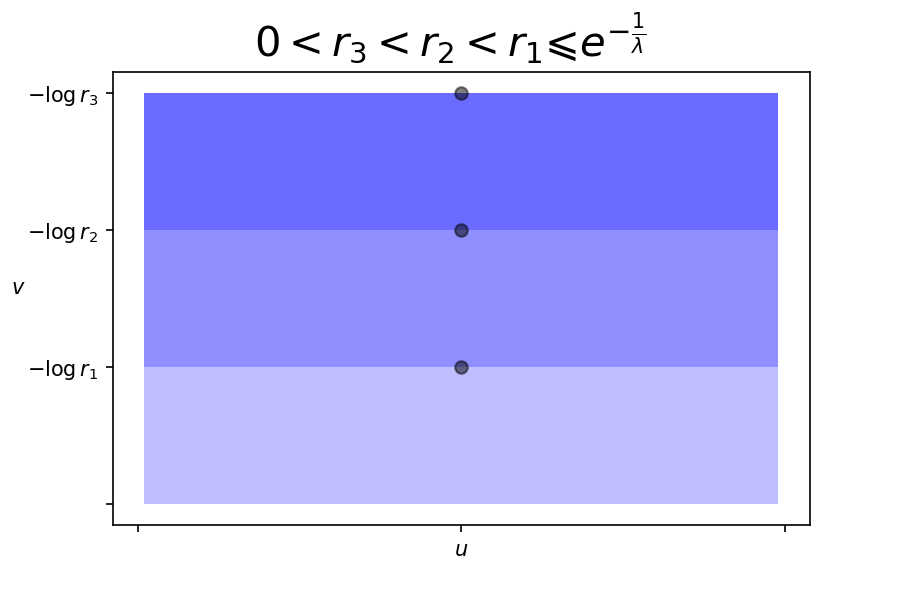
Refer to caption
Figure 13: 1r2\frac{1}{r^{2}} (The integration over v>−log⁡rv>-\log r) ≈\approx (The value at the boundary line v=log⁡rv=\log r)
Proof.

When 0<r⩽e−1λ0<r\leqslant e^{-\frac{1}{\lambda}}, which implies −log⁡r⩾1λ-\log r\geqslant\frac{1}{\lambda}, by Lemma 5.3

∫v>−log⁡rHα​(u+i​v)​‖ψα′‖2​𝑑v\displaystyle\int_{v>-\log r}H_{\alpha}(u+iv)|\!|\psi_{\alpha}^{\prime}|\!|^{2}dv =1π​∫v>−log⁡r∫y∈ℝHα​(y)​vv2+(u−y)2​2​(e−2​v+λ2​|α|2​e−2​λ​v)​𝑑y​𝑑v\displaystyle=\frac{1}{\pi}\int_{v>-\log r}\int_{y\in\mathbb{R}}H_{\alpha}(y)\frac{v}{v^{2}+(u-y)^{2}}2\,(e^{-2v}+\lambda^{2}\,|\alpha|^{2}\,e^{-2\lambda v})dy\,dv
≈1π​∫y∈ℝHα​(y)​{∫v>−log⁡r∂∂v​(vv2+(u−y)2​(−e−2​v−λ​|α|2​e−2​λ​v))​𝑑v}​𝑑y\displaystyle\approx\frac{1}{\pi}\int_{y\in\mathbb{R}}H_{\alpha}(y)\Big\{\int_{v>-\log r}\frac{\partial}{\partial v}\Big(\frac{v}{v^{2}+(u-y)^{2}}\big(-e^{-2v}-\lambda\,|\alpha|^{2}\,e^{-2\lambda v}\big)\Big)dv\Big\}\,dy
=1π​∫y∈ℝHα​(y)​−log⁡r(−log⁡r)2+(u−y)2​(r2+λ​|α|2​r2​λ)​𝑑y\displaystyle=\frac{1}{\pi}\int_{y\in\mathbb{R}}H_{\alpha}(y)\frac{-\log r}{(-\log r)^{2}+(u-y)^{2}}\big(r^{2}+\lambda\,|\alpha|^{2}\,r^{2\lambda}\big)dy
=Hα​(u+(−log⁡r)​i)​(r2+λ​|α|2​r2​λ)\displaystyle=H_{\alpha}\big(u+(-\log r)i\big)\big(r^{2}+\lambda\,|\alpha|^{2}\,r^{2\lambda}\big)
≈r2​Hα​(u+(−log⁡r)​i).\displaystyle\approx r^{2}\,H_{\alpha}\big(u+(-\log r)i\big).

For the same reason when r1−λ⩽|α|<1r^{1-\lambda}\leqslant|\alpha|<1 which implies log⁡|α|−log⁡rλ⩾−log⁡r⩾1λ\frac{\log|\alpha|-\log r}{\lambda}\geqslant-\log r\geqslant\frac{1}{\lambda}

∫v>log⁡|α|−log⁡rλHα​(u+i​v)​‖ψα′‖2​𝑑v\displaystyle\int_{v>\frac{\log|\alpha|-\log r}{\lambda}}H_{\alpha}(u+iv)|\!|\psi_{\alpha}^{\prime}|\!|^{2}dv ≈Hα​(u+(log⁡|α|−log⁡rλ)​i)​(|α|−2λ​r2λ+λ​r2)\displaystyle\approx H_{\alpha}\big(u+(\textstyle\frac{\log|\alpha|-\log r}{\lambda})i\big)\,\big(|\alpha|^{-\frac{2}{\lambda}}\,r^{\frac{2}{\lambda}}+\lambda\,r^{2})
≈r2​Hα​(u+(log⁡|α|−log⁡rλ)​i).\displaystyle\approx r^{2}\,H_{\alpha}\big(u+(\textstyle\frac{\log|\alpha|-\log r}{\lambda})i\big).

Last, when |α|⩾1|\alpha|\geqslant 1 one has −log⁡rλ⩾−log⁡r⩾1λ\frac{-\log r}{\lambda}\geqslant-\log r\geqslant\frac{1}{\lambda} and

∫v>−log⁡rλHα​(u+i​v)​‖ψα′‖2​𝑑v\displaystyle\int_{v>\frac{-\log r}{\lambda}}H_{\alpha}(u+iv)|\!|\psi_{\alpha}^{\prime}|\!|^{2}dv ≈Hα​(u+(−log⁡rλ)​i)​(|α|−2λ​r2λ+λ​r2)\displaystyle\approx H_{\alpha}\big(u+(\textstyle\frac{-\log r}{\lambda})i\big)\,\big(|\alpha|^{-\frac{2}{\lambda}}\,r^{\frac{2}{\lambda}}+\lambda\,r^{2})
≈r2​Hα​(u+(−log⁡rλ)​i).∎\displaystyle\approx r^{2}\,H_{\alpha}\big(u+(\textstyle\frac{-\log r}{\lambda})i\big).\qed

Thus

ℒ⁡(T,0)\displaystyle\mathscr{L}(T,0) ≈limr→0+{∫|α|<r1−λ∫u=02​πHα(u+(−logr)i)dudμ(α)\displaystyle\approx\lim\limits_{r\rightarrow 0+}\Big\{\int_{|\alpha|<r^{1-\lambda}}\int_{u=0}^{2\pi}H_{\alpha}\big(u+(-\log r)i\big)\,du\,d\mu(\alpha)
+∫r1−λ⩽|α|<1∫u=02​πHα(u+(log⁡|α|−log⁡rλ)i)dudμ(α)\displaystyle+\int_{r^{1-\lambda}\leqslant|\alpha|<1}\int_{u=0}^{2\pi}H_{\alpha}\big(u+(\textstyle\frac{\log|\alpha|-\log r}{\lambda})i\big)\,du\,d\mu(\alpha)
+∫|α|⩾1∫u=02​πHα(u+(−log⁡rλ)i)dudμ(α)},\displaystyle+\int_{|\alpha|\geqslant 1}\int_{u=0}^{2\pi}H_{\alpha}\big(u+(\textstyle\frac{-\log r}{\lambda})i\big)\,du\,d\mu(\alpha)\Big\},

by the inequalities (3) and (4) in the previous subsection. All terms are positive, so the order of taking limit and integration can change

ℒ⁡(T,0)\displaystyle\mathscr{L}(T,0) ≈limv→+∞∫α∈ℂ∗∫u=02​πHα​(u+i​v)​du​dμ​(α)\displaystyle\approx\lim\limits_{v\rightarrow+\infty}\int_{\alpha\in\mathbb{C}^{*}}\int_{u=0}^{2\pi}H_{\alpha}\big(u+iv\big)\,du\,d\mu(\alpha)
=limk→+∞∫α∈ℂ∗∫u=02​π∫y∈ℝHα​(y)​2​k​π(2​k​π)2+(u−y)2​dy​du​dμ​(α),\displaystyle=\lim\limits_{k\rightarrow+\infty}\int_{\alpha\in\mathbb{C}^{*}}\int_{u=0}^{2\pi}\int_{y\in\mathbb{R}}H_{\alpha}(y)\frac{2k\pi}{(2k\pi)^{2}+(u-y)^{2}}\,dy\,du\,d\mu(\alpha),

Fix some k∈ℤk\in\mathbb{Z}, k⩾2k\geqslant 2. Define intervals INI_{N} for all N∈ℤN\in\mathbb{Z} as follows

I0\displaystyle I_{0} =[−2kπ+2π,2kπ),\displaystyle=[-2k\pi+2\pi,2k\pi),
IN\displaystyle I_{N} ={[2​k​π​N,2​k​π​(N+1)),(N>0)[2kπ(N−1)+2π,2kπN+2π),(N<0)\displaystyle=\left\{\begin{aligned} &\big[2k\pi N,2k\pi(N+1)\big),&\quad{\scriptstyle{(N>0)}}\\ &\big[2k\pi(N-1)+2\pi,2k\pi N+2\pi\big),&\quad{\scriptstyle{(N<0)}}\end{aligned}\right.

Thus ℝ=⋃N∈ℤIN\mathbb{R}=\bigcup\limits_{N\in\mathbb{Z}}I_{N} is a disjoint union.

Lemma 5.5.

For any u∈(0,2​π)u\in(0,2\pi) one has

2​k​π(2​k​π)2+(u−y)2⩾11+(N+1)2​12​k​π,(y∈IN)\frac{2k\pi}{(2k\pi)^{2}+(u-y)^{2}}\geqslant\frac{1}{1+(N+1)^{2}}\frac{1}{2k\pi},\quad{\scriptstyle{(y\in I_{N})}}
Proof.

Elementary. ∎

Thus

ℒ⁡(T,0)\displaystyle\mathscr{L}(T,0) ≈limk→+∞∑N∈ℤ∫α∈ℂ∗∫u=02​π∫y∈INHα​(y)​2​k​π(2​k​π)2+(u−y)2​dy​du​dμ​(α)\displaystyle\approx\lim\limits_{k\rightarrow+\infty}\sum\limits_{N\in\mathbb{Z}}\int_{\alpha\in\mathbb{C}^{*}}\int_{u=0}^{2\pi}\int_{y\in I_{N}}H_{\alpha}(y)\frac{2k\pi}{(2k\pi)^{2}+(u-y)^{2}}\,dy\,du\,d\mu(\alpha)
⩾limk→+∞∑N∈ℤ∫α∈ℂ∗∫y∈IN∫u=02​πHα​(y)​11+(N+1)2​12​k​π​du​dy​dμ​(α)\displaystyle\geqslant\lim\limits_{k\rightarrow+\infty}\sum\limits_{N\in\mathbb{Z}}\int_{\alpha\in\mathbb{C}^{*}}\int_{y\in I_{N}}\int_{u=0}^{2\pi}H_{\alpha}(y)\frac{1}{1+(N+1)^{2}}\frac{1}{2k\pi}\,du\,dy\,d\mu(\alpha)
=limk→+∞∑N∈ℤ∫α∈ℂ∗∫y∈INHα​(y)​11+(N+1)2​1k​dy​dμ​(α).\displaystyle=\lim\limits_{k\rightarrow+\infty}\sum\limits_{N\in\mathbb{Z}}\int_{\alpha\in\mathbb{C}^{*}}\int_{y\in I_{N}}H_{\alpha}(y)\frac{1}{1+(N+1)^{2}}\frac{1}{k}\,dy\,d\mu(\alpha).

By Lemma 5.2

∫α∈ℂ∗∫y∈I0Hα​(y)​dy​dμ​(α)\displaystyle\int_{\alpha\in\mathbb{C}^{*}}\int_{y\in I_{0}}H_{\alpha}(y)\,dy\,d\mu(\alpha) =(2​k−1)​‖T‖𝔻2\displaystyle=(2k-1)\,|\!|T|\!|_{\mathbb{D}^{2}}
⩾k​‖T‖𝔻2,\displaystyle\geqslant k\,|\!|T|\!|_{\mathbb{D}^{2}},
∫α∈ℂ∗∫y∈INHα​(y)​dy​dμ​(α)\displaystyle\int_{\alpha\in\mathbb{C}^{*}}\int_{y\in I_{N}}H_{\alpha}(y)\,dy\,d\mu(\alpha) =k​‖T‖𝔻2,(N≠0).\displaystyle=k\,|\!|T|\!|_{\mathbb{D}^{2}},\quad{\scriptstyle{(N\neq 0)}}.

Thus

ℒ⁡(T,0)≳limk→+∞∑N∈ℤ11+(N+1)2​‖T‖𝔻2≈||T||𝔻2\mathscr{L}(T,0)\gtrsim\lim\limits_{k\rightarrow+\infty}\sum\limits_{N\in\mathbb{Z}}\frac{1}{1+(N+1)^{2}}\,|\!|T|\!|_{\mathbb{D}^{2}}\approx|\!|T|\!|_{\mathbb{D}^{2}}

is nonzero.

6 Case λ<0\lambda<0. Periodic current, including all currents when λ∈ℚ<0\lambda\in\mathbb{Q}_{<0}

For any α∈ℂ∗\alpha\in\mathbb{C}^{*} fixed, the leaf LαL_{\alpha} is contained in a real 3-dimensional analytic Levi-flat CR manifold |w|=|α|​|z|λ|w|=|\alpha|\,|z|^{\lambda}, which can be viewed as a curve in |z|,|w||z|,|w| coordinates. The norms |z||z| and |w||w| depends only on vv. No leaf LαL_{\alpha} tends to the singularity (0,0)(0,0). For rr sufficiently small, the leaf LαL_{\alpha} is outside of r​𝔻2r\,\mathbb{D}^{2}.

Refer to caption
Figure 14: Case λ<0\lambda<0

Like the case λ>0\lambda>0, when one fixes |z|=r|z|=r for some r∈(0,1)r\in(0,1), then |w|=|α|​|z|λ|w|=|\alpha|\,|z|^{\lambda} is uniquely determined and the real 2-dimensional leaf LαL_{\alpha} becomes a real 1-dimensional curve Lα,r:=Lα∩𝕋r2L_{\alpha,r}:=L_{\alpha}\cap\mathbb{T}^{2}_{r} on the torus 𝕋r2:={(z,w)∈𝔻2||z|=r,|w|=|α|rλ}\mathbb{T}^{2}_{r}:=\{(z,w)\in\mathbb{D}^{2}~|~|z|=r,|w|=|\alpha|\,r^{\lambda}\}. It is a closed curve if λ∈ℚ\lambda\in\mathbb{Q}, a dense curve on 𝕋r2\mathbb{T}^{2}_{r} if λ∉ℚ\lambda\notin\mathbb{Q}.

Let TT be a harmonic current directed by ℱ\mathscr{F}. Then T|PαT|_{P_{\alpha}} has the form hα​(z,w)​[Pα]h_{\alpha}(z,w)[P_{\alpha}]. Let Hα:=hα∘ψα​(u+i​v)H_{\alpha}:=h_{\alpha}\circ\psi_{\alpha}(u+iv). It is a positive harmonic function for μ\mu-almost all α∈𝔻∗\alpha\in\mathbb{D}^{*} defined on a neighborhood of a horizontal strip {(u,v)∈ℝ2|0<v<log⁡|α|λ}\{(u,v)\in\mathbb{R}^{2}~|~0<v<\frac{\log|\alpha|}{\lambda}\}.

Like what happened in the case λ>0\lambda>0, one only calculates the mass on an open subset U:={(z,w)∈𝔻2|z∉ℝ⩾0,w≠0}U:=\{(z,w)\in\mathbb{D}^{2}~|~z\notin\mathbb{R}_{\geqslant 0},w\neq 0\}. For each α∈𝔻∗\alpha\in\mathbb{D}^{*} one normalizes HαH_{\alpha} by setting Hα​(0)=1H_{\alpha}(0)=1 to fix the expression of T:=∫hα​[Pα]​𝑑μ​(α)T:=\int h_{\alpha}[P_{\alpha}]d\mu(\alpha). Similar to Lemma 5.2, for each k0∈ℤk_{0}\in\mathbb{Z} fixed,

‖T‖𝔻2\displaystyle|\!|T|\!|_{\mathbb{D}^{2}} =∫0<|α|<1∫v=0log⁡|α|λ∫u=2​k0​π2​k0​π+2​πHα​(u+i​v)​ 2​(e−2​v+λ2​|α|2​e−2​λ​v)​du​dv​dμ​(α)\displaystyle=\int_{0<|\alpha|<1}\int_{v=0}^{\frac{\log|\alpha|}{\lambda}}\int_{u=2\,k_{0}\,\pi}^{2\,k_{0}\,\pi+2\,\pi}H_{\alpha}(u+iv)\,2\,(e^{-2v}+\lambda^{2}\,|\alpha|^{2}\,e^{-2\lambda\,v})\,du\,dv\,d\mu(\alpha)
ℒ⁡(T,0)\displaystyle\mathscr{L}(T,0) =limr→0+1r2​‖T‖r​𝔻2\displaystyle=\lim\limits_{r\rightarrow 0+}\frac{1}{r^{2}}|\!|T|\!|_{r\mathbb{D}^{2}}
=limr→0+1r2​∫0<|α|<r1−λ∫v=−log⁡rlog⁡|α|−log⁡rλ∫u=2​k0​π2​k0​π+2​πHα​(u+i​v)​ 2​(e−2​v+λ2​|α|2​e−2​λ​v)​du​dv​dμ​(α)\displaystyle=\lim\limits_{r\rightarrow 0+}\frac{1}{r^{2}}\int_{0<|\alpha|<r^{1-\lambda}}\int_{v=-\log r}^{\frac{\log|\alpha|-\log r}{\lambda}}\int_{u=2\,k_{0}\,\pi}^{2\,k_{0}\,\pi+2\,\pi}H_{\alpha}(u+iv)\,2\,(e^{-2v}+\lambda^{2}\,|\alpha|^{2}\,e^{-2\lambda\,v})\,du\,dv\,d\mu(\alpha) d​y​d​x​d​μ​(α)\displaystyle\ \ \ \ \ \ \ \ \ \ \ \ \ \ \ \ \ \ \ \ \ \ \ \ \ \ \ \ \ \ \ \ \ \ \ \ \ \ \ \ \ \ \ \ \ \ \ \ \ \ \ \ \ \ \ \ \ \ \ \ \ \ \ \ \ \ \ \ \ \ \ \ \ \ \ \ \ \ \ \ \ \ \ \ \ \ \ \ \ \ \ \ \ \ \ \ \ \ \ \ \ \ dy\,dx\,d\mu(\alpha)

Now assume TT is periodic, we treat Theorem 1.5. Suppose that there exists some b∈ℤ⩽1b\in\mathbb{Z}_{\leqslant 1} such that Hα​(u+i​v)=Hα​(u+2​π​b+i​v)H_{\alpha}(u+iv)=H_{\alpha}(u+2\pi b+iv) for all α∈𝔻∗\alpha\in\mathbb{D}^{*} and all (u,v)(u,v) in a neighborhood of the strip {(u+iv)∈ℂ|u∈ℝ,v∈[0,log⁡|α|λ]}\{(u+iv)\in\mathbb{C}~|~u\in\mathbb{R},v\in[0,\frac{\log|\alpha|}{\lambda}]\}. Like Lemma 4.1, one proves

Lemma 6.1.

Let F⁡(u,v)F(u,v) be a positive harmonic function on a neighborhood of the horizontal strip {(u+iv)∈ℂ|u∈ℝ,v∈[0,C]}\{(u+iv)\in\mathbb{C}~|~u\in\mathbb{R},v\in[0,C]\} for some C>0C>0. Suppose F⁡(u,v)=F⁡(u+2​π​b,v)F(u,v)=F(u+2\pi b,v) on this strip. Then

F⁡(u,v)=∑k∈ℤ,k≠0(ak​ek​vb​cos⁡(k​ub)+bk​ek​vb​sin⁡(k​ub))+a0​(1−C−1​v)+b0​v,F(u,v)=\sum\limits_{k\in\mathbb{Z},k\neq 0}\big(a_{k}\,e^{\frac{kv}{b}}\cos(\tfrac{ku}{b})+b_{k}\,e^{\frac{kv}{b}}\sin(\tfrac{ku}{b})\big)+a_{0}\,(1-C^{-1}\,v)+b_{0}\,v,

for some ak,bk∈ℝa_{k},b_{k}\in\mathbb{R} with a0⩾0a_{0}\geqslant 0 and b0⩾0b_{0}\geqslant 0.

Proof.

The proof is almost the same as that of Lemma 4.1. Using Fourier series and calculating Laplacian, one concludes that

F⁡(u,v)=∑k∈ℤ,k≠0(ak​ek​vb​cos⁡(k​ub)+bk​ek​vb​sin⁡(k​ub))+p+q​v,F(u,v)=\sum\limits_{k\in\mathbb{Z},k\neq 0}\big(a_{k}\,e^{\frac{kv}{b}}\cos(\tfrac{ku}{b})+b_{k}\,e^{\frac{kv}{b}}\sin(\tfrac{ku}{b})\big)+p+q\,v,

for some ak,bk,p,q∈ℝa_{k},b_{k},p,q\in\mathbb{R}. For any v∈[0,C]v\in[0,C], F⁡(u,v)⩾0F(u,v)\geqslant 0 implies

∫u=02​π​bF⁡(u,v)​𝑑u=2​π​b​(p+q​v)⩾0.\int_{u=0}^{2\pi b}F(u,v)du=2\pi b\,(p+q\,v)\geqslant 0.

Thus p⩾0p\geqslant 0 and q⩾−C−1​pq\geqslant-C^{-1}\,p. One may write p+q​v=p⁡(1−C−1​v)+(q+C−1​p)​vp+q\,v=p\,(1-C^{-1}\,v)+(q+C^{-1}\,p)\,v with p=:a0⩾0p=:a_{0}\geqslant 0 and q+C−1​p=:b0⩾0q+C^{-1}\,p=:b_{0}\geqslant 0.∎

For periodic currents one may assume

Hα​(u+i​v)=∑k∈ℤ,k≠0(ak​(α)​ek​vb​cos⁡(k​ub)+bk​(α)​ek​vb​sin⁡(k​ub))+a0​(α)​(1−λlog⁡|α|​v)+b0​(α)​v,\displaystyle H_{\alpha}(u+iv)=\sum\limits_{k\in\mathbb{Z},k\neq 0}\big(a_{k}(\alpha)\,e^{\frac{kv}{b}}\cos(\tfrac{ku}{b})+b_{k}(\alpha)\,e^{\tfrac{kv}{b}}\sin(\tfrac{ku}{b})\big)+a_{0}(\alpha)\,(1-\textstyle\frac{\lambda}{\log|\alpha|}\,v)+b_{0}(\alpha)\,v, (6)

for some ak​(α),bk​(α)∈ℝa_{k}(\alpha),b_{k}(\alpha)\in\mathbb{R} with a0​(α)⩾0a_{0}(\alpha)\geqslant 0 and b0​(α)⩾0b_{0}(\alpha)\geqslant 0. According to Lemma 5.2, for any k0∈ℤk_{0}\in\mathbb{Z}, use the jacobian (5)

‖T‖𝔻2=∫0<|α|<1∫v=0log⁡|α|λ∫u=2​k0​π2​k0​π+2​πHα​(u+i​v)​ 2​(e−2​v+λ2​|α|2​e−2​λ​v)​𝑑u​𝑑v​𝑑μ​(α).|\!|T|\!|_{\mathbb{D}^{2}}=\int_{0<|\alpha|<1}\int_{v=0}^{\frac{\log|\alpha|}{\lambda}}\int_{u=2k_{0}\pi}^{2k_{0}\pi+2\pi}H_{\alpha}(u+iv)\,2\,(e^{-2v}+\lambda^{2}\,|\alpha|^{2}\,e^{-2\lambda\,v})\,du\,dv\,d\mu(\alpha).

Next, using 0=∫02​π​bcos⁡(k​ub)​𝑑u0=\int_{0}^{2\pi b}\cos(\frac{ku}{b})du for k≠0k\neq 0 and the same for sin⁡(k​ub)\sin(\frac{ku}{b}), let us calculate the average among k0=0,1,…,b−1k_{0}=0,1,\dots,b-1 for the mass

‖T‖𝔻2\displaystyle|\!|T|\!|_{\mathbb{D}^{2}} =1b​∫0<|α|<1∫v=0log⁡|α|λ∫u=02​π​bHα​(u+i​v)​ 2​(e−2​v+λ2​|α|2​e−2​λ​v)​du​dv​dμ​(α)\displaystyle=\frac{1}{b}\int_{0<|\alpha|<1}\int_{v=0}^{\frac{\log|\alpha|}{\lambda}}\int_{u=0}^{2\pi b}H_{\alpha}(u+iv)\,2\,(e^{-2v}+\lambda^{2}\,|\alpha|^{2}\,e^{-2\lambda\,v})\,du\,dv\,d\mu(\alpha)
=2​π​bb​∫0<|α|<1∫v=0log⁡|α|λ(a0​(α)​(1−λlog⁡|α|​v)+b0​(α)​v)​ 2​(e−2​v+λ2​|α|2​e−2​λ​v)​dv​dμ​(α),\displaystyle=\frac{2\pi b}{b}\int_{0<|\alpha|<1}\int_{v=0}^{\frac{\log|\alpha|}{\lambda}}\left(a_{0}(\alpha)\,(1-\textstyle\frac{\lambda}{\log|\alpha|}\,v)+b_{0}(\alpha)\,v\right)\,2\,(e^{-2v}+\lambda^{2}\,|\alpha|^{2}\,e^{-2\lambda\,v})\,dv\,d\mu(\alpha),

and for the Lelong number

ℒ⁡(T,0)\displaystyle\mathscr{L}(T,0) =limr→0+1r2​‖T‖r​𝔻2\displaystyle=\lim\limits_{r\rightarrow 0+}\frac{1}{r^{2}}|\!|T|\!|_{r\mathbb{D}^{2}}
=limr→0+1b​r2​∫0<|α|<r1−λ∫v=−log⁡rlog⁡|α|−log⁡rλ∫u=02​π​bHα​(u+i​v)​ 2​(e−2​v+λ2​|α|2​e−2​λ​v)​du​dv​dμ​(α)\displaystyle=\lim\limits_{r\rightarrow 0+}\frac{1}{b\,r^{2}}\int_{0<|\alpha|<r^{1-\lambda}}\int_{v=-\log r}^{\frac{\log|\alpha|-\log r}{\lambda}}\int_{u=0}^{2\pi b}H_{\alpha}(u+iv)\,2\,(e^{-2v}+\lambda^{2}\,|\alpha|^{2}\,e^{-2\lambda\,v})\,du\,dv\,d\mu(\alpha)
=limr→0+2​π​bb​r2​∫0<|α|<r1−λ∫v=−log⁡rlog⁡|α|−log⁡rλ(a0​(α)​(1−λlog⁡|α|​v)+b0​(α)​v)​ 2​(e−2​v+λ2​|α|2​e−2​λ​v)​dv​dμ​(α).\displaystyle=\lim\limits_{r\rightarrow 0+}\frac{2\pi b}{b\,r^{2}}\int_{0<|\alpha|<r^{1-\lambda}}\int_{v=-\log r}^{\frac{\log|\alpha|-\log r}{\lambda}}\left(a_{0}(\alpha)\,(1-\textstyle\frac{\lambda}{\log|\alpha|}\,v)+b_{0}(\alpha)\,v\right)\,2\,(e^{-2v}+\lambda^{2}\,|\alpha|^{2}\,e^{-2\lambda\,v})\,dv\,d\mu(\alpha).

Introduce the two functions of r∈(0,1]r\in(0,1] given by elementary integrals

Ia​(r)\displaystyle I_{a}(r) :=1r2​∫v=−log⁡rlog⁡|α|−log⁡rλ2​(1−λlog⁡|α|​v)​(e−2​v+λ2​|α|2​e−2​λ​v)​dv,\displaystyle:=\frac{1}{r^{2}}\int_{v=-\log r}^{\frac{\log|\alpha|-\log r}{\lambda}}2\,(1-\textstyle\frac{\lambda}{\log|\alpha|}\,v)\,(e^{-2v}+\lambda^{2}\,|\alpha|^{2}\,e^{-2\lambda\,v})\,dv,
=1+λ​|α|2​r2​λ−2+12​log⁡|α|​(−2​|α|−2λ​r2λ−2​log⁡(r)+λ​|α|−2λ​r2λ−2+2​λ2​|α|2​r2​λ−2​log⁡(r)−λ​|α|2​r2​λ−2),\displaystyle=1+\lambda\,|\alpha|^{2}\,r^{2\lambda-2}+\frac{1}{2\log|\alpha|}\left(-2|\alpha|^{-\frac{2}{\lambda}}r^{\frac{2}{\lambda}-2}\log(r)+\lambda|\alpha|^{-\frac{2}{\lambda}}r^{\frac{2}{\lambda}-2}+2\,\lambda^{2}\,|\alpha|^{2}\,r^{2\lambda-2}\log(r)-\lambda\,|\alpha|^{2}\,r^{2\lambda-2}\right),
Ib​(r)\displaystyle I_{b}(r) :=1r2​∫v=−log⁡rlog⁡|α|−log⁡rλ2​v​(e−2​v+λ2​|α|2​e−2​λ​v)​𝑑v\displaystyle:=\frac{1}{r^{2}}\int_{v=-\log r}^{\frac{\log|\alpha|-\log r}{\lambda}}2\,v\,(e^{-2v}+\lambda^{2}\,|\alpha|^{2}\,e^{-2\lambda\,v})\,dv
=12​(−|α|−2λ​r2λ−2​(λ+2​log⁡|α|−2​log⁡(r))λ+|α|2​r2​λ−2​(1−2​λ​log⁡(r))−2​log⁡|α|),\displaystyle=\frac{1}{2}\left(-\frac{|\alpha|^{-\frac{2}{\lambda}}r^{\frac{2}{\lambda}-2}(\lambda+2\log|\alpha|-2\log(r))}{\lambda}+|\alpha|^{2}r^{2\lambda-2}(1-2\lambda\log(r))-2\log|\alpha|\right),

to describe the contributions from a0​(α)a_{0}(\alpha) part and from b0​(α)b_{0}(\alpha) part.

Refer to caption
Figure 15: The green = the blue dotted (gives Ia​(r)I_{a}(r)) + the yellow dashed (gives Ib​(r)I_{b}(r))

Then we can express

‖T‖𝔻2\displaystyle|\!|T|\!|_{\mathbb{D}^{2}} =2​π​∫0<|α|<1(a0​(α)​Ia​(1)+b0​(α)​Ib​(1))​dμ​(α),\displaystyle=2\,\pi\,\int_{0<|\alpha|<1}\Big(a_{0}(\alpha)\,I_{a}(1)+b_{0}(\alpha)\,I_{b}(1)\Big)\,d\mu(\alpha),
ℒ⁡(T,0)\displaystyle\mathscr{L}(T,0) =2​π​limr→0+∫0<|α|<r1−λ(a0​(α)​Ia​(r)+b0​(α)​Ib​(r))​dμ​(α).\displaystyle=2\,\pi\,\lim\limits_{r\rightarrow 0+}\int_{0<|\alpha|<r^{1-\lambda}}\Big(a_{0}(\alpha)\,I_{a}(r)+b_{0}(\alpha)\,I_{b}(r)\Big)\,d\mu(\alpha).

Observe that

Ia​(1)\displaystyle I_{a}(1) =1+λ​|α|2+λ⁡(|α|−2λ−|α|2)2​log⁡|α|,\displaystyle=1+\lambda\,|\alpha|^{2}+\frac{\lambda\left(|\alpha|^{-\frac{2}{\lambda}}-|\alpha|^{2}\right)}{2\log|\alpha|},
Ib​(1)\displaystyle I_{b}(1) =12​(−|α|−2λ​(λ+2​log⁡|α|)λ+|α|2−2​log⁡|α|).\displaystyle=\frac{1}{2}\left(-\frac{|\alpha|^{-\frac{2}{\lambda}}(\lambda+2\log|\alpha|)}{\lambda}+|\alpha|^{2}-2\log|\alpha|\right).

Fix any α∈𝔻∗\alpha\in\mathbb{D}^{*}, by definition r2​Ia​(r)r^{2}I_{a}(r) and r2​Ib​(r)r^{2}I_{b}(r) are increasing for r∈(0,1]r\in(0,1], since the interval of integration (−log⁡r,log⁡|α|−log⁡rλ)(-\log r,\frac{\log|\alpha|-\log r}{\lambda}) is expanding and the function integrated is positive. In particular, for any r∈(0,1]r\in(0,1],

Ia​(r)⩽r−2​Ia​(1),Ib​(r)⩽r−2​Ib​(1).I_{a}(r)\leqslant r^{-2}\,I_{a}(1),\ \ \ \ I_{b}(r)\leqslant r^{-2}\,I_{b}(1).

It is more subtle to talk about monotonicity of Ia​(r)I_{a}(r) and Ib​(r)I_{b}(r). We expect upper bounds of Ia​(r)/Ia​(1)I_{a}(r)/I_{a}(1) and Ib​(r)/Ib​(1)I_{b}(r)/I_{b}(1) for r∈(0,1]r\in(0,1] which are independent of α\alpha, i.e. depend only on λ\lambda.

Lemma 6.2.

For any r∈(0,1)r\in(0,1) and any α∈ℂ\alpha\in\mathbb{C} with 0<|α|<r1−λ<10<|\alpha|<r^{1-\lambda}<1, one has

0<Ia​(r)<Ia​(1).0<I_{a}(r)<I_{a}(1).
Proof.

A differentiation gives

dd​r​Ia​(r)\displaystyle\frac{d}{dr}I_{a}(r) =|α|−2λλ​r3​log⁡|α|⏟>0​(λ2​(|α|2+2λ​r2​λ−r2λ)−2​(1−λ)​(λ3​|α|2+2λ​r2​λ+r2λ)​log⁡(r)CLOSE\displaystyle=\underbrace{\frac{|\alpha|^{-\frac{2}{\lambda}}}{\lambda\,r^{3}\,\log|\alpha|}}_{>0}\Big(\lambda^{2}\big(|\alpha|^{2+\frac{2}{\lambda}}r^{2\lambda}-r^{\frac{2}{\lambda}}\big)-2(1-\lambda)\big(\lambda^{3}|\alpha|^{2+\frac{2}{\lambda}}r^{2\lambda}+r^{\frac{2}{\lambda}}\big)\log(r)
OPEN−2​(1−λ)​λ2​|α|2+2λ​r2​λ​log⁡|α|).\displaystyle-2(1-\lambda)\lambda^{2}|\alpha|^{2+\frac{2}{\lambda}}r^{2\lambda}\log|\alpha|\Big).

It suffices to show that dd​r​Ia​(r)>0\frac{d}{dr}I_{a}(r)>0 when r∈(0,1)r\in(0,1) and 0<|α|<r1−λ0<|\alpha|<r^{1-\lambda}.

Introduce the new variable t:=|α|r1−λ∈(0,1)t:=\frac{|\alpha|}{r^{1-\lambda}}\in(0,1). In the big parentheses, replace |α||\alpha| by t​r1−λt\,r^{1-\lambda} and log⁡|α|\log|\alpha| by log⁡(t)+(1−λ)​log⁡(r)\log(t)+(1-\lambda)\log(r)

dd​r​Ia​(r)\displaystyle\frac{d}{dr}I_{a}(r) =|α|−2λ​r2λλ​r3​log⁡|α|⏟>0​(λ2​(t2+2λ−1)−2​(1−λ)​(t2+2λ+1)​log⁡(r)CLOSE\displaystyle=\underbrace{\frac{|\alpha|^{-\frac{2}{\lambda}}\,r^{\frac{2}{\lambda}}}{\lambda r^{3}\log|\alpha|}}_{>0}\Big(\lambda^{2}(t^{2+\frac{2}{\lambda}}-1)-2\,(1-\lambda)\,(t^{2+\frac{2}{\lambda}}+1)\log(r)
OPEN−2​(1−λ)​λ2​t2+2λ​log⁡(t)⏟>0)\displaystyle\underbrace{-2\,(1-\lambda)\,\lambda^{2}\,t^{2+\frac{2}{\lambda}}\log(t)}_{>0}\Big)
>|α|−2λ​r2λλ​r3​log⁡|α|​(λ2​(t2+2λ−1)⏟⩾0​−2​(1−λ)​(t2+2λ+1)​log⁡(r)⏟>0)>0,\displaystyle>\frac{|\alpha|^{-\frac{2}{\lambda}}\,r^{\frac{2}{\lambda}}}{\lambda r^{3}\log|\alpha|}\Big(\lambda^{2}\,\underbrace{(t^{2+\frac{2}{\lambda}}-1)}_{\geqslant 0}\underbrace{-2\,(1-\lambda)\,(t^{2+\frac{2}{\lambda}}+1)\log(r)}_{>0}\Big)>0,

since λ∈[−1,0)\lambda\in[-1,0) implies t2+2λ⩾1t^{2+\frac{2}{\lambda}}\geqslant 1.∎

It is not true that Ib​(r)I_{b}(r) is increasing on (0,1](0,1], but on a smaller half-neighborhood of 00, independent of α\alpha, it is increasing. This suffice to give an upper bound of Ib​(r)/Ib​(1)I_{b}(r)/I_{b}(1).

Lemma 6.3.

For any r∈(0,e12​λ​(1−λ))r\in(0,e^{\frac{1}{2\,\lambda\,(1-\lambda)}}) and any α∈ℂ\alpha\in\mathbb{C} with 0<|α|<r1−λ<10<|\alpha|<r^{1-\lambda}<1, one has

0<Ib​(r)<Ib​(e12​λ​(1−λ))⩽e1−λ⁡(1−λ)​Ib​(1).0<I_{b}(r)<I_{b}(e^{\frac{1}{2\lambda(1-\lambda)}})\leqslant e^{\frac{1}{-\lambda\,(1-\lambda)}}\,I_{b}(1).
Proof.

A differentiation gives

dd​r​Ib​(r)\displaystyle\frac{d}{dr}I_{b}(r) =|α|−2λλ2​r3⏟>0​(−λ2​(|α|2+2λ​r2​λ−r2λ)+2​(1−λ)​(λ3​|α|2+2λ​r2​λ+r2λ)​log⁡(r)CLOSE\displaystyle=\underbrace{\frac{|\alpha|^{-\frac{2}{\lambda}}}{\lambda^{2}r^{3}}}_{>0}\Big(-\lambda^{2}\big(|\alpha|^{2+\frac{2}{\lambda}}r^{2\lambda}-r^{\frac{2}{\lambda}}\big)+2(1-\lambda)\big(\lambda^{3}|\alpha|^{2+\frac{2}{\lambda}}r^{2\lambda}+r^{\frac{2}{\lambda}}\big)\log(r)
OPEN−2​(1−λ)​r2λ​log⁡|α|)\displaystyle-2(1-\lambda)r^{\frac{2}{\lambda}}\log|\alpha|\Big)

It suffices to show that dd​r​Ib​(r)>0\frac{d}{dr}I_{b}(r)>0 when 0<r<e12​λ​(1−λ)0<r<e^{\frac{1}{2\,\lambda\,(1-\lambda)}} and 0<|α|<r1−λ0<|\alpha|<r^{1-\lambda}.

Again, introduce the variable t:=|α|r1−λ∈(0,1)t:=\frac{|\alpha|}{r^{1-\lambda}}\in(0,1) and replace α\alpha and log⁡|α|\log|\alpha| in the parentheses

dd​r​Ib​(r)\displaystyle\frac{d}{dr}I_{b}(r) =|α|−2λ​r2λλ2​r3⏟>0​(−λ2​(t2+2λ−1)+2​λ​(1−λ)​(λ2​t2+2λ+1)​log⁡(r)CLOSE\displaystyle=\underbrace{\frac{|\alpha|^{-\frac{2}{\lambda}}\,r^{\frac{2}{\lambda}}}{\lambda^{2}\,r^{3}}}_{>0}\Big(-\lambda^{2}\,(t^{2+\frac{2}{\lambda}}-1)+2\,\lambda\,(1-\lambda)\,(\lambda^{2}\,t^{2+\frac{2}{\lambda}}+1)\,\log(r)
OPEN−2​(1−λ)​log⁡(t)⏟>0)\displaystyle\ \ \ \ \ \ \ \ \ \ \ \ \ \ \ \ \ \ \underbrace{-2(1-\lambda)\log(t)}_{>0}\Big)
>|α|−2λ​r2λλ2​r3​(−λ2​(t2+2λ−1)+2​λ​(1−λ)​(λ2​t2+2λ+1)⏟<0​log⁡(r)⏟<12​λ​(1−λ)<0)\displaystyle>\frac{|\alpha|^{-\frac{2}{\lambda}}\,r^{\frac{2}{\lambda}}}{\lambda^{2}\,r^{3}}\Big(-\lambda^{2}\,(t^{2+\frac{2}{\lambda}}-1)+\underbrace{2\,\lambda\,(1-\lambda)\,(\lambda^{2}\,t^{2+\frac{2}{\lambda}}+1)}_{<0}\,\underbrace{\log(r)}_{<\frac{1}{2\lambda(1-\lambda)}<0}\Big)
>|α|−2λ​r2λλ2​r3​(−λ2​(t2+2λ−1)+λ2​t2+2λ+1)=|α|−2λ​r2λλ2​r3​(λ2+1)>0.∎\displaystyle>\frac{|\alpha|^{-\frac{2}{\lambda}}\,r^{\frac{2}{\lambda}}}{\lambda^{2}\,r^{3}}\Big(-\lambda^{2}\,(t^{2+\frac{2}{\lambda}}-1)+\lambda^{2}\,t^{2+\frac{2}{\lambda}}+1\Big)=\frac{|\alpha|^{-\frac{2}{\lambda}}\,r^{\frac{2}{\lambda}}}{\lambda^{2}\,r^{3}}\big(\lambda^{2}\,+1\big)>0.\qed
End of proof of Theorem 1.5.

From what precedes, the Lelong number is zero

ℒ⁡(T,0)\displaystyle\mathscr{L}(T,0) =2​π​limr<e12​λ​(1−λ),r→0+∫0<|α|<r1−λ(a0​(α)​Ia​(r)+b0​(α)​Ib​(r))​dμ​(α)\displaystyle=2\,\pi\,\lim\limits_{r<e^{\frac{1}{2\lambda(1-\lambda)}},r\rightarrow 0+}\int_{0<|\alpha|<r^{1-\lambda}}\big(a_{0}(\alpha)\,I_{a}(r)+b_{0}(\alpha)\,I_{b}(r)\big)\,d\mu(\alpha)
<2​π​limr→0+∫0<|α|<r1−λ(a0​(α)​Ia​(1)+b0​(α)​e1−2​λ​(1−λ)​Ib​(1))​dμ​(α)\displaystyle<2\,\pi\,\lim\limits_{r\rightarrow 0+}\int_{0<|\alpha|<r^{1-\lambda}}\big(a_{0}(\alpha)\,I_{a}(1)+b_{0}(\alpha)\,e^{\frac{1}{-2\,\lambda\,(1-\lambda)}}\,I_{b}(1)\big)\,d\mu(\alpha)
≈2​π​limr→0+∫0<|α|<r1−λ(a0​(α)​Ia​(1)+b0​(α)​Ib​(1))​dμ​(α)=0,\displaystyle\approx 2\,\pi\,\lim\limits_{r\rightarrow 0+}\int_{0<|\alpha|<r^{1-\lambda}}\big(a_{0}(\alpha)\,I_{a}(1)+b_{0}(\alpha)\,I_{b}(1)\big)\,d\mu(\alpha)=0,

since ‖T‖𝔻2=2​π​∫0<|α|<1(a0​(α)​Ia​(1)+b0​(α)​Ib​(1))​𝑑μ​(α)|\!|T|\!|_{\mathbb{D}^{2}}=2\,\pi\,\int_{0<|\alpha|<1}\big(a_{0}(\alpha)\,I_{a}(1)+b_{0}(\alpha)\,I_{b}(1)\big)\,d\mu(\alpha) is finite.∎

References

  • [1]
  • [2] Alessandrini, L.; Bassanelli, G.: Plurisubharmonic currents and their extension across analytic subsets, Forum Math. 5 (1993), no. 6, 577–602.
  • [4]
  • [5] Arnold, V.I.; Ilyashenko, Yu.S.: Ordinary differential equations, Encyclopaedia Math. Sci., 1, Dynamical systems, I, 1–148, Springer, Berlin, (1988).
  • [7]
  • [8] Berndtsson, B.; Sibony, N.: The ∂\partial equation on a positive current, Invent. math. 147 (2002), 371–428.
  • [10]
  • [11] Brjuno, A.D.: A local method of nonlinear analysis for differential equations, ”Nauka”, Moscow, (1979), 253 pp.
  • [13]
  • [14] Brunella, M.: Birational geometry of foliations, IMPA Monographs, 1 Springer, Cham, (2015). xiv+130 pp.
  • [16]
  • [17] Dinh, T.C.; Nguyên, V.A.; Sibony, N.: Heat equation and ergodic theorems for Riemann surface laminations, Math. Ann. 354 (2012), no. 1, 331–376.
  • [19]
  • [20] Dinh, T.C.; Nguyên, V.A.; Sibony, N.: Unique Ergodicity for foliations on compact Kahler surfaces, (2018), arXiv: 1811.07450v2, 50 pages
  • [22]
  • [23] Dinh, T.C.; Sibony, N.: Unique ergodicity for foliations in ℙ2\mathbb{P}^{2} with an invariant curve, Invent. Math. 211 (2018), no. 1, 1–38.
  • [24]
  • [25] Dinh, T.C.; Wu, H.: Harmonic currents directed by foliations by Riemann surfaces, (2020), arXiv: 2010.03796, 9 pages
  • [27]
  • [28] Fornæss, J.E.; Sibony, N.: Unique ergodicity of harmonic currents on singular foliations of ℙ2\mathbb{P}^{2}, Geom. Funct. Anal. 19 (2010), no. 5, 1334–1377.
  • [30]
  • [31] Fornæss, J.E.; Sibony, N.; Wold, E.F.: Examples of minimal laminations and associated currents, Math. Z. 269 (2011), no. 1-2, 495–520.
  • [33]
  • [34] Nguyên, V.A.: Directed harmonic currents near hyperbolic singularities, Ergodic Theory Dynam. Systems 38 (2018), no. 8, 3170–3187.
  • [36]
  • [37] Nguyên, V.A.: Singular holomorphic foliations by curves. III: Zero Lelong numbers, arXiv:2009.06566
  • [39]
  • [40] Nguyên, V.A.: Ergodic theorems for laminations and foliations: recent results and perspectives, Acta. Math. Vietnam. 45 (2020)
  • [42]
  • [43] Widder, D.V.: Functions harmonic in a strip, Proc. Amer. Math. Soc. 12 (1961), 67–72.
  • [45]
  • [46] Seidenberg, A.: Reduction of singularities of the differential equation A​d​y=B​d​xAdy=Bdx, Amer. J. Math. 90 (1968), 248–269.
  • [48]
  • [49] Skoda, H.: Prolongement des courants, positifs, fermés de Masse finie, (French) [Extension of closed, positive currents of finite Mass] Invent. Math. 66 (1982), no. 3, 361–376.
  • [50]

Zhangchi Chen, Université Paris-Saclay, CNRS, Laboratoire de mathématiques d’Orsay, 91405, Orsay, France
zhangchi.chen@universite-paris-saclay.fr
, https://www.imo.universite-paris-saclay.fr/∼\simchen/