Nonlocality, steering and quantum state tomography in a single experiment
Abstract
We investigate whether paradigmatic measurements for quantum state tomography, namely mutually unbiased bases and symmetric informationally complete measurements, can be employed to certify quantum correlations. For this purpose, we identify a simple and noise-robust correlation witness for entanglement detection, steering and nonlocality that can be evaluated based on the outcome statistics obtained in the tomography experiment. This allows us to perform state tomography on entangled qutrits, a test of Einstein-Podolsky-Rosen steering and a Bell inequality test, all within a single experiment. We also investigate the trade-off between quantum correlations and subsets of tomographically complete measurements as well as the quantification of entanglement in the different scenarios. Finally, we perform a photonics experiment in which we demonstrate quantum correlations under these flexible assumptions, namely with both parties trusted, one party untrusted and both parties untrusted.
Introduction.— When Alice and Bob perform local measurements on a shared two-particle quantum state, they can observe correlations that go beyond classical models. These correlations are crucial for fundamental and applied aspects of quantum information science, but their precise sense of nonclassicality hinges on the assumptions made on the measurement devices. Three seminal scenarios have been widely studied in the literature: (i) both measurement devices are trusted, (ii) one device is trusted and the other is untrusted, (iii) both devices are untrusted. Nonclassicality in these scenarios correspond to detection of entanglement Gühne and Tóth 2009, steering Uola et al. 2020 and nonlocality Brunner et al. 2014 respectively. These are the paradigmatic resources for standard Horodecki et al. 2009, one-sided device-independent Branciard et al. 2012 and fully device-independent Pironio et al. 2010 quantum information processing, respectively.
Therefore, it is important to experimentally classify states as entangled Friis et al. 2019, steerable Bennet et al. 2012; Zeng et al. 2018; Guo et al. 2019; Designolle et al. 2020 or nonlocal Shalm et al. 2015; Giustina et al. 2015; Hensen et al. 2015. Typically, this requires three different experiments because the measurements tailored for detecting one form of nonclassicality generally are not well-suited for detecting another form of nonclassicality. For instance, the measurements optimal for violating the celebrated CHSH Bell inequality do not detect the steerability of any two-qubit isotropic state that is not already nonlocal Cavalcanti et al. 2015. Another example is that correlations obtained from an optimal entanglement witness often admit a local-variable model when the measurement devices are no longer trusted.
Focusing on two-qutrit systems, we develop a correlation witness that detects quantum correlations in all three scenarios (i-iii) simultaneously. Our nonclassicality criteria are strongly noise tolerant and can be implemented using a flexible number of measurements on each side. We experimentally demonstrate their usefulness by detecting entanglement, steering and nonlocality for increasingly noisy states in a single experiment. Moreover, we show that the same data also can be used to deduce quantitative bounds on the entanglement in scenarios (i-iii).
Our protocol is based on mutually unbiased bases (MUBs) Durt et al. 2010 and symmetric informationally complete measurements (SICs) Zauner 2011; Renes et al. 2004. Two bases are said to be MUBs if the magnitude of the overlap between any two basis elements chosen from different bases is constant. A set of MUBs in dimension is tomographically complete Wootters and Fields 1989. Similarly, a tomographically complete set of pure states is called a SIC if the overlap between any two states has the same magnitude. MUBs and SICs are conceptually related Wootters 2006; Bengtsson 2010; Bengtsson et al. 2012; Beneduci et al. 2013; Tavakoli et al. 2020a) and optimal for quantum state tomography Wootters and Fields 1989; Scott 2006; Řeháček et al. 2004; which has prompted experimental demonstrations Adamson and Steinberg 2010; Giovannini et al. 2013; Medendorp et al. 2011; Pimenta et al. 2013; Bent et al. 2015; Hou et al. 2015; Hou et al. 2018; Tang et al. 2020.
In scenario (i), tomographically complete measurements enable full reconstruction of the quantum state and thus the evaluation of any entanglement criterion. Similarly, in scenario (ii), such measurements are important for local reconstruction of the state assemblages, enabling optimal steering criteria. However, beyond some notable special cases based on qubits Gisin 2007; Tavakoli and Gisin 2020, there are no known Bell inequalities for which both complete sets of MUBs and SICs are optimal choices of measurements. Here, we present such a Bell inequality.
State tomography via MUBs and SIC.— Let Alice and Bob share an unknown three-dimensional bipartite system whose density matrix they wish to estimate. To this end, they perform state tomography Leonhardt and Paul 1995; Paris and Řeháček 2005. Alice performs one of nine dichotomic measurements which respectively correspond to a projection onto each of the (unnormalised) states in the following SIC:
| (1) |
where . A successful projection corresponds to the outcome and otherwise to the outcome . We label the measurements by a pair of trits, , where labels the row and labels the column in (1). Equivalently, we can use the label . Bob measures in one of the four (unnormalised) MUBs
| (2) |
where the columns represent the basis states. The columns in a given basis thus represent his outcome, labelled . The measurement basis is labelled by two bits, , which we equivalently write as . The probabilities can be used to reconstruct the state by standard methods (see e.g. Ref. Schmied 2016).
Correlation witness.— First noticed already in 1844 Hesse 1844, the SIC (1) and the MUBs (2) exhibit a remarkable geometric relationship (see also Ref. Bengtsson et al. 2012). If a system is prepared in any of the nine states (1) and subsequently measured in any of the four bases (2), the probability distribution over the three possible outcomes admits a simple structure: one outcome can never occur and the other two are equiprobable. The events that cannot occur are characterised by the relation when and when . We define when this relation is satisfied and otherwise. This observation can be extended to entangled system. If the shared state is maximally entangled, a local projection onto any of the elements in the SIC remotely prepares the other system in the same state (up to transpose). Inspired by this, we define a simple witness of the observed correlations:
| (3) |
Consider now that Alice and Bob share the maximally entangled state exposed to a degree of isotropic noise: , where is the visibility. If Alice and Bob perform the measurements (1) and (2) respectively, one obtains , which in the noise-free case () becomes . In what follows, we show that these quantum correlations detect nonclassicality in the scenarios (i-iii).
Correlation inequalities.— Based on the witness , we construct a Bell inequality, a steering inequality and an entanglement witness. For the first, we distrust Alice’s and Bob’s devices and determine the largest value of compatible with a local-hidden-variable (LHV) model: , where is the local variable Brunner et al. 2014. By considering all vertices of the polytope formed by these correlations Fine 1982, one finds a tight Bell inequality. For the second, we distrust only (say) Alice’s device and assume that Bob performs the measurements (2). The (unnormalised) local states of Bob after Alice’s measurements are given by the assemblage , where are Alice’s measurement operators. We determine the largest value of compatible with a local-hidden-state (LHS) model Wiseman et al. 2007: where are quantum states. This is achieved through a semidefinite program (see SM). For the third, we trust both devices and determine the largest value of compatible with a separable (SEP) state: , where and are pure qutrit states. This can be achieved by relaxing the set of separable states to the set of states with a positive partial transpose Horodecki et al. 1996 and then evaluating a semidefinite program (see SM). Then, we have saturated the resulting bound with a separable state to ensure tightness.
In this manner, we obtain the tight correlation inequalities
| (4) |
We see that gradually relaxing the assumptions on Alice’s and Bob’s devices leads to stronger correlations in the relevant classical models. The last inequality (proven in SM) is a bound respected by quantum correlations for arbitrary states and local measurements. Note that this coincides with the value obtained from the SIC and MUBs.
The Bell inequality in (4) is violated whenever . No better Bell inequality is possible for because for any smaller the full distribution can be simulated in a local-variable model. To further explore the role of tomographically complete measurements in our Bell inequality test, we have numerically searched for the largest value of possible with real Hilbert spaces of a fixed dimension. For qutrits, we found at best 11 1 By increasing the Hilbert space dimension to five, we could still not find a maximal violation in real Hilbert spaces (). In dimension six, one can achieve in real spaces.. This illustrates the need for exploiting the full structure of qutrit Hilbert space.
If the isotropic state is too noisy () to violate the Bell inequality, we can instead violate the steering inequality in (4) if . Interestingly, the critical visibility can be further reduced by fine-graining the witness. In our quantum protocol, the marginal distribution of Alice is regardless of the visibility . Hence, the second term in (3) is . If we fix , the analysis of the quantum protocol remains unchanged but the bound for LHS models is reduced to . This allows us to detect steering for . Importantly, this threshold cannot be further reduced by using any other witness since it equals that obtained from considering full tomography of . Notably, the visibility threshold is lower than that encountered for a two-qubit isotropic state under general projective measurements () Wiseman et al. 2007. Furthermore, it is not far from the threshold limiting the most general experiment based on any number of dichotomic projective measurements, namely Nguyen and Gühne 2020; Wiseman et al. 2007. Finally, we have also considered the reverse situation in which Alice is trusted and Bob is untrusted. Then, the witness detects steering for (see also Ref. Bavaresco et al. 2017).
If the isotropic state is too noisy to violate the steering inequality, we can instead violate the separable bound in (4) if . Note that this is optimal, because below this visibility, the isotropic state is separable Horodecki et al. 1996.
The above analysis, based on , provides a simple criterion that applies equally well to detecting three forms of nonclassicality in manner that is optimal for the isotropic state in our input/output scenario. However, it is often relevant to detect quantum correlations in a more resource-efficient way; by using fewer measurements. Next, we go beyond the inequalities (4) and consider quantum correlations in the full statistics when the number of settings on Alice and Bob is a degree of freedom.
Correlations from fewer settings.— We investigate the trade-off between efficient nonclassicality criteria (using few measurements) and stronger criteria (using more measurements). For this purpose, a natural setting is to let Alice and Bob measure only subsets of the elements in the SIC and MUBs respectively, i.e. to use only settings and for some and . If small choices of are insufficient to detect the nonclassicality of a state, additional elements of the SIC and MUBs can be measured, thus step-by-step approaching a tomographically complete set Bae et al. 2019. In SM, we employ convex programming methods to determine visibility thresholds for the state above which the probability distribution , for given , implies entanglement, steering and nonlocality respectively. In particular, we find that entanglement is detected already in the minimal scenario, , albeit at high visibility. We illustrate in Table 1 the results when and Alice performs only measurements. For entanglement, the detection is optimal already at . Steering is robustly detected already at . However, nonlocality requires at least .
| 2 | 3 | 4 | 5 | 6 | 7 | 8 | 9 | |
|---|---|---|---|---|---|---|---|---|
| SEP | 0.63 | 0.40 | 0.36 | 0.31 | 0.25 | 0.25 | 0.25 | 0.25 |
| LHS | 0.73 | 0.67 | 0.60 | 0.56 | 0.53 | 0.51 | 0.49 | 0.47 |
| LHV | - | - | - | 0.91 | 0.86 | 0.86 | 0.81 | 0.75 |
Entanglement quantification.— Our above results classify a state as either entangled, steerable or nonlocal. We now go further and show that entanglement also can be quantified, specifically through the entanglement negativity Vidal and Werner 2002, based on the observed quantum correlations, in a standard, one-sided device-independent and fully device-independent manner respectively. The negativity is defined as , where denotes partial transpose. It can alternatively be computed as the semidefinite program .
In the trusted scenario (i), we consider the case of and , which we previously found was the minimal setting for optimal detection of the isotropic state. For given , we solve the semidefinite program for under the additional constraint that all probabilities are reproduced by the state when applying the SIC and MUBs. For , we find the bound . When , our numerical bound can be approximated up to the third decimal by the polynomial . A non-trivial amount of entanglement is quantified for every nontrivial visibility.
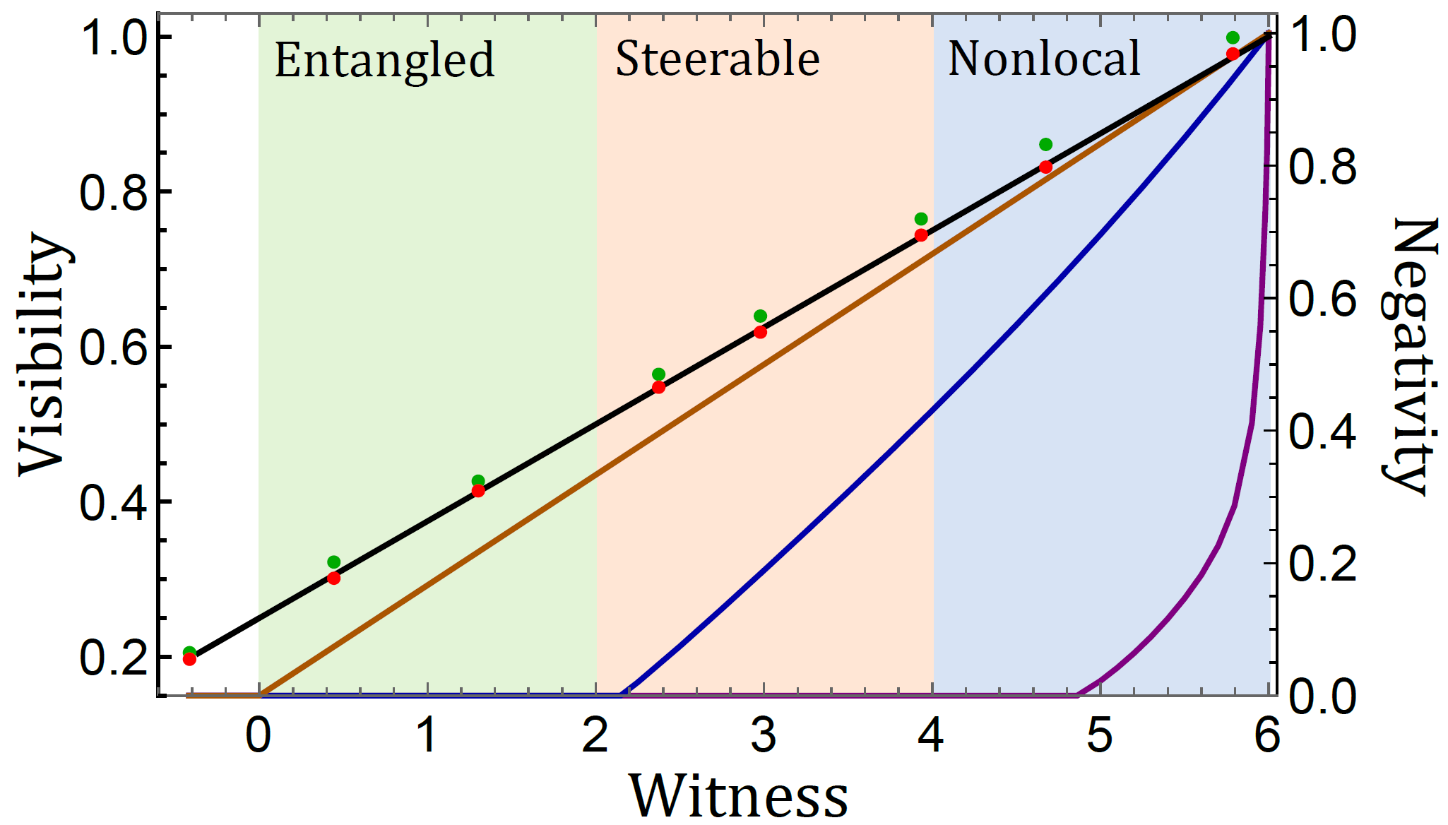
In the one-sided device-independent scenario (ii) and in the fully device-independent scenario (iii), we quantify entanglement based on the parameter used in the steering and Bell inequalities in (4). This can be achieved using the semidefinite relaxation hierarchies in Ref. Pusey 2013 and Ref. Moroder et al. 2013 respectively. By using a level intermediate between the first and second, we have obtained non-trivial bounds on . These are displayed in Figure 2. For completeness, we also illustrate in Figure 2 the bound for the trusted scenario (i) using tomographically complete measurements. For the ideal case of , all our numerical bounds return the optimal negativity . However, below (steering) and (nonlocality) respectively, we have , which is suboptimal. The reason is that since we work with enough settings for tomographic completeness, and go beyond a qubit scenario, it is computationally expensive to consider semidefinite relaxations sufficiently large to obtain nearly-optimal bounds. It is likely that already the evaluation of the second relaxation level will improve the bounds for scenarios (ii) and (iii).

Experimental setup.— We have demonstrated nonlocality, steering and tomography in a photonics experiment. The setup (see Fig. 1) is composed of three parts. The first part is the preparation of the isotropic state , which is encoded in both the polarisation and the path degree of freedom of the photons. The horisontal-polarisation (vertical-polarisation) photon taking path () encodes the state , the vertical-polarisation (horisontal-polarisation) photon taking path () encodes the state and the horisontal-polarisation (vertical-polarisation) photon passing path () encodes the state . The maximally entangled state is generated through the type-II phase-matched spontaneous parametric down-conversion (SPDC) process in the Sagnac structure Guo et al. 2019. The visibility parameter is controlled by inserting quartz crystals to destroy the coherence of a photon-pair state Verbanis et al. 2016.
The second part is the realisation of Alice’s measurements (see Fig. 1). Alice can choose between performing one of nine different binary-outcome measurements, corresponding to the SIC (1), on her qutrit. These measurements are realised by three half-wave plates (HWPs), six quarter-wave plates (QWPs), one beam displacer (BD), a polarisation beam splitter (PBS) and three single photon detectors. The detector is used to record the outcome and the detectors and record the outcome .
The third part is the realisation of Bob’s measurements (see Fig. 1). The four MUBs (2) are realised using five HWPs, six QWP, two BDs, a PBS and three single photon detectors. The detector , and are used to record outcomes respectively. The wave-plate angles corresponding to Alice’s and Bob’s measurements are given in SM.
Experimental results.— We have realised the isotropic state for eight different target visibilities. For each case, we perform the measurements (1) and (2) with approximately shots per setting . In SM we use the relative frequencies to estimate the density matrix via the maximum-likelihood method Ježek et al. 2003. The visibility of the reconstructed matrix is, however, somewhat smaller than our targeted visibility (see SM), primarily due to imperfections in the source and the interference between the BDs. For instance, when we target the preparation of the maximally entangled state (), the visibility of the reconstructed state is approximately .
In Fig. 2, we present the measured value of the witness for the different visibilities; green (red) points are target (estimated) visibilities. The standard deviations are all of a magnitude smaller than , corresponding to accumulated statistical and systematic errors. Systematic errors include that our coincidence rate is approximately per second of which roughly one is a dark count, that the wave-plates are subject to a small offset () and induce a phase error (). The solid black line represents the theoretical witness value . We see that our data accurately confirms the theoretical prediction. When the visibility is high we observe that the data violates the Bell inequality in Eq. (4). To this end, we assume fair-sampling in the detection events. When the visibility is further reduced, the data violates the steering inequality in Eq. (4). For even smaller visibilities, we still detect entanglement through the witness in Eq. (4). For our final data point (with target visibility ), the isotropic state is separable. For instance, when no noise is deliberately added to the system (target ), we observe . This certifies a negativity of in the steering scenario, which is only marginally worse than computed from the reconstructed density matrix. In the Bell scenario, our value of certifies at least . Also, the witness value exceeds the largest value found using quantum theory constrained to real three-dimensional systems and real five-dimensional systems by and standard deviations respectively.
Discussion.— We have performed quantum state tomography on increasingly noisy entangled states via mutually unbiased bases and symmetric informationally complete projections. Using a simple correlation witness, we showed that the outcome statistics can be re-interpreted both as a demonstration of steering and a demonstration of nonlocality. Moreover, we showed how classification of nonclassical properties can be achieved using a tunable number of measurements and that entanglement can be quantified in the three scenarios using a single setup.
Our work, together with the foundational interest in Bell inequalities tailored for important quantum measurements Kaniewski et al. 2019; Tavakoli et al. 2019, motivates a natural open problem: to generalise our findings to MUBs and SICs of any dimension. It interesting to investigate how the noise-tolerance of such a generalisation scales with the system dimension and the choice of assumption. For practical purposes, this is particularly relevant for steering since witnesses of our type only use binary-outcome measurements for the untrusted party (Alice). This facilitates experimental implementation while simultaneously, e.g. for the isotropic state, does not imply a significant fundamental constraint on the detectable states Nguyen and Gühne 2020.
Finally, another interesting continuation of our work is to develop noise-robust correlation witnesses for detection of nonlocality, steering and entanglement in quantum networks Tavakoli et al. 2021. In such networks, in analogy with our approach here, it is known that measurements in MUBs and entangled measurements based on SICs are natural candidates to reveal quantum nonlocality Gisin 2019; Tavakoli et al. 2020b; Bäumer et al. 2020.
Acknowledgements.
We thank Roope Uola and Jędrzej Kaniewski for comments and discussions. We are obliged to Ingemar Bengtsson for inspiration. This work was supported by the Swiss National Science Foundation (Starting grant DIAQ, NCCR-SwissMAP and Early PostDoc Mobility fellowship P2GEP2 194800), the National Natural Science Foundation of China under Grants (Nos. 11574291, 11774334, 11874345 and 11904357), the National Key Research and Development Program of China (No.2017YFA0304100, No.2018YFA0306400), Key Research Program of Frontier Sciences, CAS (No.QYZDY-SSW-SLH003), Science and Technological Fund of Anhui Province for Outstanding Youth (2008085J02).References
- Gühne and Tóth (2009) O. Gühne and G. Tóth, Physics Reports 474, 1 (2009).
- Uola et al. (2020) R. Uola, A. C. S. Costa, H. C. Nguyen, and O. Gühne, Rev. Mod. Phys. 92, 015001 (2020).
- Brunner et al. (2014) N. Brunner, D. Cavalcanti, S. Pironio, V. Scarani, and S. Wehner, Rev. Mod. Phys. 86, 419 (2014).
- Horodecki et al. (2009) R. Horodecki, P. Horodecki, M. Horodecki, and K. Horodecki, Rev. Mod. Phys. 81, 865 (2009).
- Branciard et al. (2012) C. Branciard, E. G. Cavalcanti, S. P. Walborn, V. Scarani, and H. M. Wiseman, Phys. Rev. A 85, 010301 (2012).
- Pironio et al. (2010) S. Pironio, A. Acín, S. Massar, A. B. de la Giroday, D. N. Matsukevich, P. Maunz, S. Olmschenk, D. Hayes, L. Luo, T. A. Manning, and C. Monroe, Nature 464, 1021 (2010).
- Friis et al. (2019) N. Friis, G. Vitagliano, M. Malik, and M. Huber, Nature Reviews Physics 1, 72 (2019).
- Bennet et al. (2012) A. J. Bennet, D. A. Evans, D. J. Saunders, C. Branciard, E. G. Cavalcanti, H. M. Wiseman, and G. J. Pryde, Phys. Rev. X 2, 031003 (2012).
- Zeng et al. (2018) Q. Zeng, B. Wang, P. Li, and X. Zhang, Phys. Rev. Lett. 120, 030401 (2018).
- Guo et al. (2019) Y. Guo, S. Cheng, X. Hu, B.-H. Liu, E.-M. Huang, Y.-F. Huang, C.-F. Li, G.-C. Guo, and E. G. Cavalcanti, Phys. Rev. Lett. 123, 170402 (2019).
- Designolle et al. (2020) S. Designolle, V. Srivastav, R. Uola, N. H. Valencia, W. McCutcheon, M. Malik, and N. Brunner, Genuine high-dimensional quantum steering (2020), arXiv:2007.02718v1, 2007.02718 .
- Shalm et al. (2015) L. K. Shalm, E. Meyer-Scott, B. G. Christensen, P. Bierhorst, M. A. Wayne, M. J. Stevens, T. Gerrits, S. Glancy, D. R. Hamel, M. S. Allman, K. J. Coakley, S. D. Dyer, C. Hodge, A. E. Lita, V. B. Verma, C. Lambrocco, E. Tortorici, A. L. Migdall, Y. Zhang, D. R. Kumor, W. H. Farr, F. Marsili, M. D. Shaw, J. A. Stern, C. Abellán, W. Amaya, V. Pruneri, T. Jennewein, M. W. Mitchell, P. G. Kwiat, J. C. Bienfang, R. P. Mirin, E. Knill, and S. W. Nam, Phys. Rev. Lett. 115, 250402 (2015).
- Giustina et al. (2015) M. Giustina, M. A. M. Versteegh, S. Wengerowsky, J. Handsteiner, A. Hochrainer, K. Phelan, F. Steinlechner, J. Kofler, J.-Å. Larsson, C. Abellán, W. Amaya, V. Pruneri, M. W. Mitchell, J. Beyer, T. Gerrits, A. E. Lita, L. K. Shalm, S. W. Nam, T. Scheidl, R. Ursin, B. Wittmann, and A. Zeilinger, Phys. Rev. Lett. 115, 250401 (2015).
- Hensen et al. (2015) B. Hensen, H. Bernien, A. E. Dréau, A. Reiserer, N. Kalb, M. S. Blok, J. Ruitenberg, R. F. L. Vermeulen, R. N. Schouten, C. Abellán, W. Amaya, V. Pruneri, M. W. Mitchell, M. Markham, D. J. Twitchen, D. Elkouss, S. Wehner, T. H. Taminiau, and R. Hanson, Nature 526 (2015).
- Cavalcanti et al. (2015) E. G. Cavalcanti, C. J. Foster, M. Fuwa, and H. M. Wiseman, J. Opt. Soc. Am. B 32, A74 (2015).
- Durt et al. (2010) T. Durt, B.-G. Englert, I. Bengtsson, and K. Życzkowski, International Journal of Quantum Information 08, 535 (2010).
- Zauner (2011) G. Zauner, International Journal of Quantum Information 09, 445 (2011), https://doi.org/10.1142/S0219749911006776 .
- Renes et al. (2004) J. M. Renes, R. Blume-Kohout, A. J. Scott, and C. M. Caves, Journal of Mathematical Physics 45, 2171 (2004), https://doi.org/10.1063/1.1737053 .
- Wootters and Fields (1989) W. K. Wootters and B. D. Fields, Annals of Physics 191, 363 (1989).
- Wootters (2006) W. K. Wootters, Foundations of Physics 36, 112 (2006).
- Bengtsson (2010) I. Bengtsson, Journal of Physics: Conference Series 254, 012007 (2010).
- Bengtsson et al. (2012) I. Bengtsson, K. Blanchfield, and A. Cabello, Physics Letters A 376, 374 (2012).
- Beneduci et al. (2013) R. Beneduci, T. J. Bullock, P. Busch, C. Carmeli, T. Heinosaari, and A. Toigo, Phys. Rev. A 88, 032312 (2013).
- Tavakoli et al. (2020a) A. Tavakoli, I. Bengtsson, N. Gisin, and J. M. Renes, Phys. Rev. Research 2, 043122 (2020a).
- Scott (2006) A. J. Scott, Journal of Physics A: Mathematical and General 39, 13507 (2006).
- Řeháček et al. (2004) J. Řeháček, B.-G. Englert, and D. Kaszlikowski, Phys. Rev. A 70, 052321 (2004).
- Adamson and Steinberg (2010) R. B. A. Adamson and A. M. Steinberg, Phys. Rev. Lett. 105, 030406 (2010).
- Giovannini et al. (2013) D. Giovannini, J. Romero, J. Leach, A. Dudley, A. Forbes, and M. J. Padgett, Phys. Rev. Lett. 110, 143601 (2013).
- Medendorp et al. (2011) Z. E. D. Medendorp, F. A. Torres-Ruiz, L. K. Shalm, G. N. M. Tabia, C. A. Fuchs, and A. M. Steinberg, Phys. Rev. A 83, 051801 (2011).
- Pimenta et al. (2013) W. M. Pimenta, B. Marques, T. O. Maciel, R. O. Vianna, A. Delgado, C. Saavedra, and S. Pádua, Phys. Rev. A 88, 012112 (2013).
- Bent et al. (2015) N. Bent, H. Qassim, A. A. Tahir, D. Sych, G. Leuchs, L. L. Sánchez-Soto, E. Karimi, and R. W. Boyd, Phys. Rev. X 5, 041006 (2015).
- Hou et al. (2015) Z. Hou, G. Xiang, D. Dong, C.-F. Li, and G.-C. Guo, Opt. Express 23, 10018 (2015).
- Hou et al. (2018) Z. Hou, J.-F. Tang, J. Shang, H. Zhu, J. Li, Y. Yuan, K.-D. Wu, G.-Y. Xiang, C.-F. Li, and G.-C. Guo, Nature Communications 9, 1414 (2018).
- Tang et al. (2020) J.-F. Tang, Z. Hou, J. Shang, H. Zhu, G.-Y. Xiang, C.-F. Li, and G.-C. Guo, Phys. Rev. Lett. 124, 060502 (2020).
- Gisin (2007) N. Gisin, Bell inequalities: many questions, a few answers, In essays in honour of Abner Shimony, Eds Wayne C. Myrvold and Joy Christian, The Western Ontario Series in Philosophy of Science, pp 125-140, Springer 2009 (2007), arXiv:quant-ph/0702021v2, quant-ph/0702021 .
- Tavakoli and Gisin (2020) A. Tavakoli and N. Gisin, Quantum 4, 293 (2020).
- Leonhardt and Paul (1995) U. Leonhardt and H. Paul, Progress in Quantum Electronics 19, 89 (1995).
- Paris and Řeháček (2005) M. Paris and J. Řeháček, Quantum State Estimation (Springer, 2005).
- Schmied (2016) R. Schmied, Journal of Modern Optics 63, 1744 (2016), https://doi.org/10.1080/09500340.2016.1142018 .
- Hesse (1844) O. Hesse, J. Reine Angew. Math. 28 (1844).
- Fine (1982) A. Fine, Phys. Rev. Lett. 48, 291 (1982).
- Wiseman et al. (2007) H. M. Wiseman, S. J. Jones, and A. C. Doherty, Phys. Rev. Lett. 98, 140402 (2007).
- Horodecki et al. (1996) M. Horodecki, P. Horodecki, and R. Horodecki, Physics Letters A 223, 1 (1996).
- Nguyen and Gühne (2020) H. C. Nguyen and O. Gühne, Some quantum measurements with three outcomes can reveal nonclassicality where all two-outcome measurements fail (2020), arXiv:2001.03514v1, 2001.03514 .
- Bavaresco et al. (2017) J. Bavaresco, M. T. Quintino, L. Guerini, T. O. Maciel, D. Cavalcanti, and M. T. Cunha, Phys. Rev. A 96, 022110 (2017).
- Bae et al. (2019) J. Bae, B. C. Hiesmayr, and D. McNulty, New Journal of Physics 21, 013012 (2019).
- Vidal and Werner (2002) G. Vidal and R. F. Werner, Phys. Rev. A 65, 032314 (2002).
- Pusey (2013) M. F. Pusey, Phys. Rev. A 88, 032313 (2013).
- Moroder et al. (2013) T. Moroder, J.-D. Bancal, Y.-C. Liang, M. Hofmann, and O. Gühne, Phys. Rev. Lett. 111, 030501 (2013).
- Verbanis et al. (2016) E. Verbanis, A. Martin, D. Rosset, C. C. W. Lim, R. T. Thew, and H. Zbinden, Phys. Rev. Lett. 116, 190501 (2016).
- Ježek et al. (2003) M. Ježek, J. Fiurášek, and Z. c. v. Hradil, Phys. Rev. A 68, 012305 (2003).
- Kaniewski et al. (2019) J. Kaniewski, I. Šupić, J. Tura, F. Baccari, A. Salavrakos, and R. Augusiak, Quantum 3, 198 (2019).
- Tavakoli et al. (2019) A. Tavakoli, M. Farkas, D. Rosset, J.-D. Bancal, and J. Kaniewski, Mutually unbiased bases and symmetric informationally complete measurements in Bell experiments (2019), arXiv:1912.03225v2, 1912.03225 .
- Tavakoli et al. (2021) A. Tavakoli, A. Pozas-Kerstjens, M.-X. Luo, and M.-O. Renou, Bell nonlocality in networks (2021), arXiv:2104.10700v1, 2104.10700 .
- Gisin (2019) N. Gisin, Entropy 21, 325 (2019).
- Tavakoli et al. (2020b) A. Tavakoli, N. Gisin, and C. Branciard, Bilocal Bell inequalities violated by the quantum Elegant Joint Measurement (2020b), arXiv:2006.16694v1, 2006.16694 .
- Bäumer et al. (2020) E. Bäumer, N. Gisin, and A. Tavakoli, Certification of highly entangled measurements and nonlocality via scalable entanglement-swapping on quantum computers (2020), arXiv:2009.14028v1, 2009.14028 .
Appendix A Maximal quantum violation of the Bell inequality
We prove that in quantum theory. We denote Alice’s outcome-one measurement operators by and Bob’s measurement operators by . Without loss of generality, we can restrict and to projective operators. First, we focus on just the first of the two terms in the witness, which we denote , which in a quantum model reads
| (5) |
Using the Cauchy-Schwarz inequality, we obtain
The expression under the first square-root is just the marginal probability . Let us denote it by . Then the Cauchy-Schwarz inequality gives
| (6) |
Expanding the expression under the second square-root, one finds that it is independent of Bob’s choice of measurements,
| (7) |
Using this fact, and the simplifying notation , we arrive at
| (8) |
Turning to the full witness expression , we use Eq. (8) to obtain
| (9) |
In order to evaluate the maximal value of the right-hand-side, we solve which gives . Inserted into Eq. (9), we find
| (10) |
Appendix B Nonlocality, steering and entanglement from subsets of SIC and MUBs
Consider that we perform only a subset of the measurements for quantum state tomography. Specifically, Alice performs only the first binary-outcome measurements corresponding to the SIC and Bob performs only the first MUBs. The full tomography case therefore corresponds to . How well can we detect nonlocality, steering and entanglement using only such subsets of the SIC and subsets of the complete set of MUBs?
B.1 Nonlocality
We investigate nonlocality in the measured probabilities when Alice only performs her first measurements and Bob performs the complete set of MUBs when sharing the isotropic state . We note that this analysis readily extends also to other states. We have used a linear program to evaluate the critical visibility for a simulation of in a local model. This linear program is
| (11) |
where and are all deterministic functions from Alice’s and Bob’s respective inputs to their respective outputs. Note that the probability distribution itself is a function of since it is given by measurements on the isotropic state of visibility . We have evaluated this program for every pair and found that only when and it is possible to detect nonlocality. The critical visibilities required for nonlocality are given in Table 2.
| n | 5 | 6 | 7 | 8 | 9 |
|---|---|---|---|---|---|
| v | 0.914 | 0.857 | 0.857 | 0.813 | 0.750 |
B.2 Steering
Consider that Alice is untrusted and only performs of the measurements in the SIC while Bob performs the four MUBs (). Since Bob’s measurements are tomographically complete, he can reconstruct the steering assemblage . We can determine the critical visibility for steerability by solving the following semidefinite program:
| (12) |
where are all deterministic functions mapping Alice’s input to her output and is a subnormalised state. That the final constraint in the above SDP stems from the fact that Bob’s share of the isotropic state is regardless of . Note that appears indirectly in the assemblages . Furthermore, we note that if this program certifies the state as steerable, one can always extract a steering inequality by considering the dual of the above SDP.
In Table 3 we give the critical visiblity for detecting steering for the different values of . Note that the case of coincides with the critical visibility given in the main text based on the quantity . We find that steering is detected for every . In fact, even in the case of only using two of the nine SIC projections, the visibility is lower than that required to violate our Bell inequality.
| n | 2 | 3 | 4 | 5 | 6 | 7 | 8 | 9 |
|---|---|---|---|---|---|---|---|---|
| v | 0.727 | 0.667 | 0.602 | 0.561 | 0.532 | 0.510 | 0.488 | 0.470 |
The SDP in Eq. (B.2) can be straightforwardly adapted to the opposite case, in which Alice is trusted and Bob is not. Then, we consider that Alice performs local tomography using the full set of SIC measurements while Bob measures only MUBs. In Table 4, we give the critical visibilities for steerability. We see that even two MUBs are sufficient to demonstrate steering of the isotropic state at visibilities for which no Bell inequality violation is known.
| m | 2 | 3 | 4 |
|---|---|---|---|
| v | 0.683 | 0.569 | 0.481 |
B.3 Entanglement detection
We now consider entanglement detection from the probability distribution based on the isotropic state and and measurement respectively for Alice and Bob. In contrast to the cases of nonlocality and steering, it is difficult to give a necessary and sufficient condition for whether there exists a separable model for the full distribution. We address the problem by relaxing the set of separable states to the set of quantum states with a positive partial transpose. This allows us to identify an upper bound for the critical visibility needed for entanglement detection through by solving the following semidefinite program:
| (13) |
We have evaluated this SDP for every pair and the resulting upper bounds on the critical visibility for entanglement detection is given in Table 5. We see that for every pair it is possible to detect entanglement. Moreover, we see that the required visibility reduces as we increase the number of settings on Alice or Bob. In particular, for the isotropic state, optimal entanglement detection is achieved already for and , which is more efficient than the criterion based on the quantity given in the main text.
| m\n | 2 | 3 | 4 | 5 | 6 | 7 | 8 | 9 |
|---|---|---|---|---|---|---|---|---|
| 2 | 0.9132 | 0.8117 | 0.6553 | 0.5680 | 0.5000 | 0.5000 | 0.5000 | 0.5000 |
| 3 | 0.7933 | 0.6667 | 0.5259 | 0.4288 | 0.3487 | 0.3448 | 0.3333 | 0.3333 |
| 4 | 0.6323 | 0.4000 | 0.3633 | 0.3136 | 0.2500 | 0.2500 | 0.2500 | 0.2500 |
We note that by considering the dual of the above SDP one can convert these certificates into entanglement witnesses (inequalities) that are more friendly to experimental implementation. Lastly, we remark that one could in principle hope to obtain tighter bounds on the critical visibiltiy than that provided by the relaxation (B.3). This can be achieved using the DPS hierarchy, which is based on considering symmetric extensions of states with a positive partial transpose. The SDP (B.3) corresponds to the lowest level in this hierarchy. We have also implemented the second level of the hierarchy, based on a state which is invariant under permutation of Bob’s two subsystems and which has a positive partial transpose with respect to Bob’s systems. However, for most choices of this does not improve the critical visibility and for the few cases in which and improvement is obtained, it is only a minor one.
Appendix C Wave-plate angles
In Table 6 we present the wave-plate angles for the nine measurements corresponding to the considered SIC. Similarly, the wave-plate angles corresponding to the four MUBs are given in Table 7. In particular, the angles for the unitary gate correspond to the QWP, HWP, QWP from the left to the right.
| SIC | U1 | U2 | U3 | ||||||
|---|---|---|---|---|---|---|---|---|---|
| 1 | -22.5 | 22.5 | -22.5 | 0 | 0 | 0 | 0 | 0 | 0 |
| 2 | -45 | 52.5 | 0 | 0 | 0 | 0 | 0 | 0 | 0 |
| 3 | 45 | 52.5 | 90 | 0 | 0 | 0 | 0 | 0 | 0 |
| 4 | 0 | 45 | 90 | 0 | 0 | 0 | -22.5 | 22.5 | -22.5 |
| 5 | 0 | 45 | 90 | 0 | 0 | 0 | -45 | 52.5 | 0 |
| 6 | 0 | 45 | 90 | 0 | 0 | 0 | 45 | 52.5 | 90 |
| 7 | 0 | 0 | 0 | 0 | 0 | 0 | -22.5 | 22.5 | -22.5 |
| 8 | 0 | 0 | 0 | 0 | 0 | 0 | 45 | 52.5 | 90 |
| 9 | 0 | 0 | 0 | 0 | 0 | 0 | -45 | 52.5 | 0 |
| MUB | H1 | H2 | U4 | U5 | U6 | ||||||
|---|---|---|---|---|---|---|---|---|---|---|---|
| 1 | 0 | -45 | 0 | -45 | 90 | 45 | 90 | -45 | 0 | -45 | 90 |
| 2 | 67.5 | 45 | 0 | 45 | 0 | 27.37 | -17.63 | 27.37 | 45 | 0 | 90 |
| 3 | 67.5 | 45 | 0 | 45 | 0 | 45 | 12.37 | 9.74 | -45 | -60 | 0 |
| 4 | 67.5 | 45 | 0 | 45 | 0 | 45 | -57.37 | 80.26 | 45 | 52.5 | 90 |
Appendix D Experimental tomography of prepared states
We have prepared the isotropic state for eight different target visibilities and reconstructed the density matrix using a maximum-likelihood estimate. Here, we display the results of the tomographic procedure for all eight cases (red for real part of the density matrix, blue for imaginary part of the density matrix).
(
a) b)
b)
(
(
a) b)
b)
(
(
a) b)
b)
(
(
a) b)
b)
(
(
a) b)
b)
(
(
a) b)
b)
(
(
a) b)
b)
(
(
a) b)
b)
(
Appendix E Experimental witness values
In Table 8 we present the measured values of for the eight different visibilities, corresponding to the results Figure in the main text.
| Target visibility | 0.205 | 0.323 | 0.427 | 0.567 | 0.639 | 0.765 | 0.861 | 1 |
| Estimated visibility | 0.197 | 0.303 | 0.413 | 0.547 | 0.621 | 0.742 | 0.833 | 0.977 |
| -0.418 | 0.438 | 1.304 | 2.375 | 2.985 | 3.942 | 4.667 | 5.796 | |
| 0.012 | 0.012 | 0.012 | 0.013 | 0.013 | 0.014 | 0.015 | 0.015 |