Gradient discretization of two-phase poro-mechanical models with discontinuous pressures at matrix fracture interfaces

Coupled flow and geomechanics play an important role in many subsurface processes such as water management, geothermal energy, CO₂ sequestration, oil and gas production or nuclear waste storage. This is particularly the case in the presence of fractures which have a strong impact both on the flow and on the rock mechanical behavior. This work considers the so called hybrid-dimensional or Discrete Fracture Matrix (DFM) models representing the fractures as a network of co-dimension one surfaces coupled with the surrounding matrix domain. The reduced flow model is then obtained by averaging both the unknowns and the equations in the fracture width and by imposing appropriate transmission conditions at both sides of the matrix fracture interfaces. The mechanical model is set on the matrix domain with appropriate boundary conditions on both sides of the fracture interfaces. This type of hybrid-dimensional models has been the object of intensive researches over the last twenty years due to the ubiquity of fractures in geology and their considerable impact on the flow and transport of mass and energy in porous media, and on the mechanical behavior of rocks. For the derivation and analysis of such models, let us refer to [4, 27, 40, 44, 6, 13, 15, 46] for single-phase Darcy flows, [9, 49, 45, 36, 14, 23, 16, 2] for two-phase Darcy flows, and [41, 42, 38, 33, 34, 29, 39, 30, 52, 32] for poroelastic models.

As in [10], this work focuses on a hybrid-dimensional two-phase Darcy flow model coupled with a linear poroelastic deformation of the matrix. The fractures are assumed to remain open and fully filled by the fluids, and their propagation over time is neglected. The Poiseuille law is used for the tangential velocity along the fracture network and extended to two-phase flow based on generalized Darcy laws. As in [17], the concept of equivalent pressure, used to extend the poro-mechanical coupling to two-phase flow, is based on the capillary energy density. This is a crucial choice to obtain the stability of the coupled model.

In [10], the continuity of both phase pressures is used as a transmission condition at matrix fracture interfaces. This is a classical assumption in the case of highly permeable fractures such as open fractures. As shown e.g. in [28], this choice is fully justified for the case of single-phase flows. On the other hand, in the case of two-phase flow, this assumption can lead to inaccurate solutions at the matrix fracture interfaces [16, 2]. This is in particular the case when the fractures are fully filled by one phase and act as barriers for the other phase due to its very low relative permeability within the fractures, hence leading to a pressure discontinuity. Let us refer to [2] for striking examples including the desaturation by suction at the interface between the atmosphere and a low permeable and fractured storage rock.

This potential inaccuracy of continuous pressure models motivates us to consider the extension of the analysis carried out in [10] to hybrid-dimensional discontinuous pressure flow models [36, 23, 16, 2]. For such flow models, the Darcy fluxes between the matrix fracture interface and the fracture are modelled using a two-point flux approximation combined with an upwind approximation of the mobilities [23, 16, 2]. Following [23], the model also includes a layer of damaged rock at matrix fracture interfaces. This additional accumulation term plays a major role in the numerical analysis of the model and also improves the nonlinear convergence at each time step of the simulation [23, 12]. It must be kept sufficiently small to maintain the accuracy of the solution (see [23]). Following [10] and [23], this new hybrid-dimensional poro-mechanical model is discretized using the gradient discretization method [22]. This framework is based on abstract vector spaces of discrete unknowns combined with reconstruction operators. The gradient scheme is then obtained by substitution of the continuous operators by their discrete counterparts in the weak formulation of the coupled model. The main asset of this framework is to allow a generic convergence analysis based on general properties of the reconstruction operators that hold for a large class of conforming and non conforming discretizations. Let us point out that, with respect to [10], additional trace and jump operators need to be defined in this framework, along with new definitions of coercivity, consistency, limit-conformity, and compactness. The two main ingredients to discretize the coupled model are the discretizations of the hybrid-dimensional discontinuous pressure two-phase Darcy flow and the discretization of the mechanics. Let us briefly mention, in both cases, a few families of discretizations typically satisfying the gradient discretization properties.

For the discretization of the Darcy flow, the gradient discretization framework covers the case of cell-centered finite volume schemes with Two-Point Flux Approximation on strongly admissible meshes [40, 6, 2], or some symmetric Multi-Point Flux Approximations [51, 50, 3] on tetrahedral or hexahedral meshes. It also accounts for the families of Mixed Hybrid Mimetic and Mixed or Mixed Hybrid Finite Element discretizations such as in [44, 15, 7, 32], and for vertex-based discretizations such as the Vertex Approximate Gradient scheme [15, 23, 16]. For the discretization of the elastic mechanical model, the gradient discretization framework covers conforming finite element methods such as in [33], the Crouzeix-Raviart discretization  [35, 20], the Hybrid High Order discretization  [19], and the Virtual Element Method [8].

The main objective of this work is to introduce the gradient discretization of the hybrid-dimensional poro-mechanical model with discontinuous pressure at matrix fracture interfaces. Then, we prove the convergence of the discrete solution to a weak solution of the model. Compared with [10], new difficulties arise from the interfacial additional nonlinear flux and accumulation terms including the damaged rock type. Assuming that the fracture normal transmissivity is fixed in the interfacial two-point fluxes, i.e. that its fracture aperture dependence is frozen, we are able to prove the convergence of the gradient scheme solution to a weak solution of the model. This assumption is rather mild since, in practice, the solution depends only weakly on this fracture normal transmissivity as long as it remains much larger than the matrix transmissivity. Concerning compactness estimates, the same techniques as in [10] are used: time translates, uniform-in-time $L^{2}$-weak estimates, and a discrete version of the Ascoli-Arzelà theorem. In [10], where fields defined in matrix and fracture are related, matrix and fracture contributions have to be separated by a cut-off argument (since the fracture width vanishes at tips). On the other hand, in this work, such a separation stems from the model itself, but the damaged rock layer has to be embedded in the time translates of the saturations, by using ad-hoc test functions combining the matrix and damaged layer rock types.

As in [10], the proof additionally assumes that the matrix porosity remains bounded from below by a strictly positive constant, that the fracture aperture remains larger than a fixed aperture vanishing only at the tips, and that the mobility functions are bounded from below by strictly positive constants. The assumptions on the porosity and fracture aperture cannot be avoided since the continuous model does not ensure these properties, which are needed to ensure its well-posedness. The assumption on the mobilities are classical to carry out the stability and convergence analysis of two-phase Darcy flows with heterogeneous rock types (see [26, 14, 23]).

The second objective of this work is to compare the discontinuous pressure poro-mechanical model investigated in this work to the continuous pressure poro-mechanical model presented in [10]. Two test cases are considered. As in [10], the first test case simulates the gas injection in a cross-shaped fracture network immersed in an initially water saturated porous medium. The second test case models the desaturation of a low permeable medium by suction at the interface with a ventilation tunnel. The data set of this second test case is based on the Callovo-Oxfordian argilite rock properties of the nuclear waste storage prototype facility of Andra. The geometry uses an axisymmetric DFM model based on a simplified version of the fracture network at the interface between the storage rock and the ventilation tunnel. In both cases the discretization is based on the Two-Point Flux Approximation finite volume scheme for the flows and second-order finite elements for the mechanical deformation.

The rest of the article is organized as follows. Section 2 introduces the continuous hybrid-dimensional coupled model with discontinuous pressures at matrix fracture interfaces. Section 3 describes the gradient discretization method for the coupled model including the definition of the reconstruction operators, the discrete variational formulation and the properties of the gradient discretization needed for the subsequent convergence analysis. Section 4 proceeds with the convergence analysis. The a priori estimates are established in Subsection 4.1, the compactness properties in Subsection 4.2 and the convergence to a weak solution is proved in Subsection 4.3. This convergence falls short, in general, from identifying the limit matrix–fracture nonlinear fluxes; this issue is discussed in Subsection 4.4, in which an assumption is given on the limit fracture width under which the fluxes can be fully identified. In Section 5, devoted to numerical experiments, the discontinuous pressure model is compared to the continuous pressure model presented in [10].

We consider a bounded polytopal domain $\Omega$ of $\mathbb R^{d}$, $d\in\{2,3\}$, partitioned into a fracture domain $\Gamma$ and a matrix domain $\Omega\backslash\overline{\Gamma}$. The network of fractures is defined by

where each fracture $\Gamma_{i}\subset\Omega$, $i\in I$ is a planar polygonal simply connected open domain. Without restriction of generality, we will assume that the fractures may intersect exclusively at their boundaries (see Figure 1), that is, for any $i,j\in I,i\neq j$ one has $\Gamma_{i}\cap\Gamma_{j}=\emptyset$, but not necessarily $\overline{\Gamma}_{i}\cap\overline{\Gamma}_{j}=\emptyset$.

The two sides of a given fracture of $\Gamma$ are denoted by $\pm$ in the matrix domain, with unit normal vectors $\mathbf{n}^{\pm}$ oriented outward of the sides $\pm$. We denote by $\gamma_{\mathfrak{a}}$ the trace operators on the sides ${\mathfrak{a}}=\pm$ of $\Gamma$ for functions in $H^{1}(\Omega\setminus\overline{\Gamma})$, by $\gamma_{\partial\Omega}$ the trace operator for the same functions on $\partial\Omega$, and by $\llbracket\cdot\rrbracket$ the normal trace jump operator on $\Gamma$ for functions in $H_{\rm div}(\Omega\backslash\overline{\Gamma})$, defined by

We denote by $\nabla_{\tau}$ the tangential gradient and by ${\rm div}_{\tau}$ the tangential divergence on the fracture network $\Gamma$. The symmetric gradient operator $\bbespilon$ is defined such that $\bbespilon(\bar{\mathbf{v}})={1\over 2}(\nabla\bar{\mathbf{v}}+^{t}\!(\nabla\bar{\mathbf{v}}))$ for a given vector field $\bar{\mathbf{v}}\in H^{1}(\Omega\backslash\overline{\Gamma})^{d}$.

Let us fix a continuous function $d_{0}:\Gamma\to(0,+\infty)$ with zero limits at $\partial\Gamma\setminus(\partial\Gamma\cap\partial\Omega)$ (i.e. the tips of $\Gamma$) and strictly positive limits at $\partial\Gamma\cap\partial\Omega$. The fracture aperture, denoted by $\bar{d}_{f}$ and such that $\bar{d}_{f}=-\llbracket\bar{\mathbf{u}}\rrbracket$ for a displacement field $\bar{\mathbf{u}}\in H^{1}(\Omega\backslash\overline{\Gamma})^{d}$, will be assumed to satisfy the following open fracture condition

Let us introduce some relevant function spaces. First, we denote by $H_{d_{0}}^{1}(\Gamma)$ the space made of functions $v_{\Gamma}$ in $L^{2}(\Gamma)$, such that $d_{0}^{\nicefrac{{3}}{{2}}}\nabla_{\tau}v_{\Gamma}$ belongs to $L^{2}(\Gamma)^{d-1}$, and whose traces are continuous at fracture intersections $\partial\Gamma_{i}\cap\partial\Gamma_{j}$, $(i,j)\in I\times I$ ($i\neq j$) and vanish on the boundary $\partial\Gamma\cap\partial\Omega$. We then introduce the space

for the displacement vector, and

where

for each matrix phase pressure, and

for each fracture phase pressure. For $\bar{v}=(\bar{v}_{m},\bar{v}_{f})\in V^{0}$, let us denote by

the jump operator on the side ${\mathfrak{a}}=\pm$ of the fractures.

The matrix, fracture and damaged rock types are denoted by the indices ${\rm rt}=m$, ${\rm rt}=f$, and ${\rm rt}=\pm$, respectively, and the non-wetting and wetting phases by the superscripts $\alpha={\rm nw}$ and $\alpha={\rm w}$, respectively. Finally, for any $x\in\mathbb R$, we set $x^{+}=\max\{0,x\}$ and $x^{-}=-(-x)^{+}$.

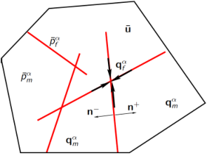
The PDEs model reads: find the phase pressures $\bar{p}^{\alpha}_{\nu}$, $\nu\in\{m,f\}$, $\alpha\in\{{\rm nw},{\rm w}\}$, and the displacement vector field $\bar{\mathbf{u}}$, such that $\bar{p}_{c,\nu}=\bar{p}_{\nu}^{\rm nw}-\bar{p}_{\nu}^{\rm w}$, and for $\alpha\in\{{\rm nw},{\rm w}\}$,

with the coupling conditions

the initial conditions

and normal flux conservation for $\mathbf{q}^{\alpha}_{f}$ at fracture intersections not located at the boundary $\partial\Omega$. Above, the equivalent pressure $\bar{p}^{E}_{\nu}$, $\nu\in\{m,f\}$ is defined, following [17], by

where

is the capillary energy density function for each rock type ${\rm rt}\in\{m,f,\pm\}$. As already noticed in [42, 38, 10], this is a key choice to obtain the energy estimates that are the starting point for the convergence analysis.

We make the following main assumptions on the data:

1. (H1)

   For each phase $\alpha\in\{{\rm nw},{\rm w}\}$ and rock type ${\rm rt}\in\{m,f,\pm\}$, the mobility function $\eta^{\alpha}_{\rm rt}$ is continuous, non-decreasing, and there exist $0<\eta_{\rm rt,{\rm min}}^{\alpha}\leq\eta^{\alpha}_{\rm rt,{\rm max}}<+\infty$ such that $\eta^{\alpha}_{\rm rt,{\rm min}}\leq\eta^{\alpha}_{\rm rt}(s)\leq\eta^{\alpha}_{\rm rt,{\rm max}}$ for all $s\in[0,1]$.

2. (H2)

   For each rock type ${\rm rt}\in\{m,f,\pm\}$, the non-wetting phase saturation function $S^{\rm nw}_{\rm rt}$ is a non-decreasing Lipschitz continuous function with values in $[0,1]$, and $S^{\rm w}_{\rm rt}=1-S^{\rm nw}_{\rm rt}$.

3. (H3)

   For ${\mathfrak{a}}=\pm$, the width $\bar{d}_{\mathfrak{a}}$ and porosity $\bar{\phi}_{\mathfrak{a}}$ of the damaged rock are strictly positive constants.

4. (H4)

   $b\in[0,1]$ is the Biot coefficient, $M>0$ is the Biot modulus, and $\lambda>0$, $\mu>0$ are the Lamé coefficients. These coefficients are assumed to be constant for simplicity.

5. (H5)

   The initial matrix porosity satisfies $\bar{\phi}_{m}^{0}\in L^{\infty}(\Omega)$.

6. (H6)

   The initial pressures are such that $(\bar{p}^{\alpha}_{0,m},\bar{p}^{\alpha}_{0,f})\in V^{0}$, $p^{\alpha}_{0,m}\in L^{\infty}(\Omega)$ and $\bar{p}^{\alpha}_{0,f}\in L^{\infty}(\Gamma)$, $\alpha\in\{{\rm nw},{\rm w}\}$.

7. (H7)

   The source terms satisfy $\mathbf{f}\in L^{2}(\Omega)^{d}$, $h_{m}^{\alpha}\in L^{2}((0,T)\times\Omega),$ and $h_{f}^{\alpha}\in L^{2}((0,T)\times\Gamma)$.

8. (H8)

   The normal fracture transmissivity $T_{f}\in L^{\infty}(\Gamma)$ is uniformly bounded from below by a strictly positive constant.

9. (H9)

   The matrix permeability tensor $\mathbb{K}_{m}$ is symmetric and uniformly elliptic on $\Omega$.

Let us denote by $C_{c}^{\infty}([0,T)\times\Omega\setminus\overline{\Gamma})$ the space of smooth functions $\bar{v}:[0,T]\times(\Omega\setminus\overline{\Gamma})\to\mathbb R$ vanishing on $\partial\Omega$ and at $t=T$, and whose derivatives of any order admit finite limits on each side of $\Gamma$. We will also use the boldface notation $\mathbf{C}_{c}^{\infty}([0,T]\times\Omega\setminus\overline{\Gamma})$ for $C_{c}^{\infty}([0,T)\times\Omega\setminus\overline{\Gamma})^{d}$.

The gradient discretization (GD) for the Darcy discontinuous pressure model, introduced in [23], is defined by a finite-dimensional vector space of discrete unknowns

and

• •

  two discrete gradient linear operators on the matrix and fracture domains

  $$\nabla_{\mathcal{D}_{p}}^{m}:X^{0}_{\mathcal{D}_{p}^{m}}\rightarrow L^{\infty}(\Omega)^{d},\quad\quad\nabla_{\mathcal{D}_{p}}^{f}:X^{0}_{\mathcal{D}_{p}^{f}}\rightarrow L^{\infty}(\Gamma)^{d-1},$$

• •

  two function reconstruction linear operators on the matrix and fracture domains

  $$\Pi_{\mathcal{D}_{p}}^{m}:X^{0}_{\mathcal{D}_{p}^{m}}\rightarrow L^{\infty}(\Omega),\quad\quad\Pi_{\mathcal{D}_{p}}^{f}:X^{0}_{\mathcal{D}_{p}^{f}}\rightarrow L^{\infty}(\Gamma),$$

• •

  for ${\mathfrak{a}}=\pm$, jump reconstruction linear operators $\llbracket\cdot\rrbracket^{\mathfrak{a}}_{\mathcal{D}_{p}}$: $X^{0}_{\mathcal{D}_{p}}\rightarrow L^{\infty}(\Gamma)$, and trace reconstruction linear operators $\mathbb{T}^{\mathfrak{a}}_{\mathcal{D}_{p}}$: $X^{0}_{\mathcal{D}_{p}^{m}}\rightarrow L^{\infty}(\Gamma)$.

The operators $\Pi_{\mathcal{D}_{p}}^{m}$, $\Pi_{\mathcal{D}_{p}}^{f}$, $\mathbb{T}^{\mathfrak{a}}_{\mathcal{D}_{p}}$ are assumed piecewise constant [22, Definition 2.12]. A consequence of the piecewise-constant property is the following: there is a basis $(\mathbf{e}_{i})_{i\in I}$ of $X^{0}_{\mathcal{D}_{p}^{m}}$ such that, if $v=\sum_{i\in I}v_{i}\mathbf{e}_{i}$ and if, for a mapping $g:\mathbb R\to\mathbb R$ with $g(0)=0$, we define $g(v)=\sum_{i\in I}g(v_{i})\mathbf{e}_{i}\in X^{0}_{\mathcal{D}_{p}^{m}}$ by applying $g$ component-wise, then $\Pi_{\mathcal{D}_{p}}^{m}g(v)=g(\Pi_{\mathcal{D}_{p}}^{m}v)$ and $\mathbb{T}_{\mathcal{D}_{p}}^{{\mathfrak{a}}}g(v)=g(\mathbb{T}_{\mathcal{D}_{p}}^{\mathfrak{a}}v)$. Note that the basis $(\mathbf{e}_{i})_{i\in I}$ is usually canonical and chosen in the design of $X^{0}_{\mathcal{D}_{p}^{m}}$. The same property holds for $X^{0}_{\mathcal{D}_{p}^{f}}$ and $\Pi_{\mathcal{D}_{p}}^{f}$. The vector space $X^{0}_{\mathcal{D}_{p}}$ is endowed with the following quantity, assumed to define a norm:

The gradient discretization for the mechanics is defined by a finite-dimensional vector space of discrete unknowns $X^{0}_{\mathcal{D}_{\mathbf{u}}}$ and

• •

  a discrete symmetric gradient linear operator $\bbespilon_{\mathcal{D}_{\mathbf{u}}}:X^{0}_{\mathcal{D}_{\mathbf{u}}}\rightarrow L^{2}(\Omega,\mathcal{S}_{d}(\mathbb R))$ where $\mathcal{S}_{d}(\mathbb R)$ is the vector space of real symmetric matrices of size $d$,

• •

  a displacement function reconstruction linear operator $\Pi_{\mathcal{D}_{\mathbf{u}}}:X^{0}_{\mathcal{D}_{\mathbf{u}}}\rightarrow L^{2}(\Omega)^{d}$,

• •

  a normal jump function reconstruction linear operator $\llbracket\cdot\rrbracket_{\mathcal{D}_{\mathbf{u}}}:X^{0}_{\mathcal{D}_{\mathbf{u}}}\rightarrow L^{4}(\Gamma)$.

Let us define the divergence operator ${\rm div}_{\mathcal{D}_{\mathbf{u}}}(\cdot)=\mbox{\rm Trace}(\bbespilon_{\mathcal{D}_{\mathbf{u}}}(\cdot))$, the stress tensor operator

and the fracture width $d_{f,\mathcal{D}_{\mathbf{u}}}=-\llbracket\mathbf{u}\rrbracket_{\mathcal{D}_{\mathbf{u}}}$. It is assumed that the following quantity defines a norm on $X^{0}_{\mathcal{D}_{\mathbf{u}}}$:

A spatial GD can be extended into a space-time GD by complementing it with

• •

  a discretization $0=t_{0}<t_{1}<\dots<t_{N}=T$ of the time interval $[0,T]$,

• •

  interpolators $I^{\nu}_{\mathcal{D}_{p}}\colon V_{\nu}^{0}\rightarrow X^{0}_{\mathcal{D}_{p}^{\nu}}$, $\nu\in\{m,f\}$, and $J^{m}_{\mathcal{D}_{p}}\colon L^{2}(\Omega)\rightarrow X^{0}_{\mathcal{D}_{p}^{m}}$ of initial conditions.

For $n\in\{0,\ldots,N\}$, we denote by $\delta t^{n+\frac{1}{2}}=t_{n+1}-t_{n}$ the time steps, and by $\Delta t=\max_{n=0,\ldots,N}\delta t^{n+\frac{1}{2}}$ the maximum time step.

Spatial operators are extended into space-time operators as follows. Let $\Psi_{\mathcal{D}}$ be a spatial GDM operator defined in $X_{\mathcal{D}}^{0}$ with $\mathcal{D}=\mathcal{D}_{\mathbf{u}}$, $\mathcal{D}_{p}^{m}$ or $\mathcal{D}_{p}^{f}$, and let $w=(w_{n})_{n=0}^{N}\in(X^{0}_{\mathcal{D}})^{N+1}$. Then, its space-time extension is defined by

For convenience, the same notation is kept for the spatial and space-time operators. Moreover, we define the discrete time derivative as follows: for $f:[0,T]\to L^{1}(\Omega)$ piecewise constant on the time discretization, with $f_{n}=f_{|(t_{n-1},t_{n}]}$ and $f_{0}=f(0)$, we set $\delta_{t}f(t)=\frac{f_{n+1}-f_{n}}{\delta t^{n+\frac{1}{2}}}$ for all $t\in(t_{n},t_{n+1}]$, $n\in\{0,\ldots,N-1\}$.

Notice that the space of piecewise constant $X^{0}_{\mathcal{D}}$-valued functions $f$ on the time discretization together with the initial value $f_{0}=f(0)$ can be identified with $(X^{0}_{\mathcal{D}})^{N+1}$. The same definition of discrete derivative can thus be given for an element $w\in(X^{0}_{\mathcal{D}})^{N+1}$. Namely, $\delta_{t}w\in(X^{0}_{\mathcal{D}})^{N}$ is defined by setting, for any $n\in\{0,\ldots,N-1\}$ and $t\in(t_{n},t_{n+1}]$, $\delta_{t}w(t)=(\delta_{t}w)_{n+1}\coloneqq\frac{w_{n+1}-w_{n}}{\delta t^{n+\frac{1}{2}}}$. If $\Psi_{\mathcal{D}}$ is a space-time GDM operator, by linearity the following commutativity property holds: $\Psi_{\mathcal{D}}\delta_{t}w(t,\cdot)=\delta_{t}(\Psi_{\mathcal{D}}w(t,\cdot))$.

The gradient scheme for (3) consists in writing the weak formulation (6a)–(6b) with continuous spaces and operators substituted by their discrete counterparts, after a formal integration by part: find $p^{\alpha}=(p^{\alpha}_{m},p^{\alpha}_{f})\in(X^{0}_{\mathcal{D}_{p}})^{N+1}$, $\alpha\in\{{\rm nw},{\rm w}\}$, and $\mathbf{u}\in(X^{0}_{\mathcal{D}_{\mathbf{u}}})^{N+1}$, such that for all $\varphi^{\alpha}=(\varphi^{\alpha}_{m},\varphi^{\alpha}_{f})\in(X_{\mathcal{D}_{p}}^{0})^{N+1}$, $\mathbf{v}\in(X^{0}_{\mathcal{D}_{\mathbf{u}}})^{N+1}$ and $\alpha\in\{{\rm nw},{\rm w}\}$,

The initial conditions are given by $p^{\alpha}_{0,\nu}=I^{\nu}_{\mathcal{D}_{p}}\bar{p}^{\alpha}_{0,\nu}$ ($\alpha\in\{{\rm nw},{\rm w}\}$, $\nu\in\{m,f\}$), $\phi_{m}^{0}=J_{\mathcal{D}_{p}}^{m}\bar{\phi}^{0}$, and the initial displacement $\mathbf{u}^{0}$ is the solution in $X^{0}_{\mathcal{D}_{\mathbf{u}}}$ of (8) without the time variable and with the equivalent pressures obtained from the initial pressures $(p^{\alpha}_{0})_{\alpha\in\{{\rm nw},{\rm w}\}}$.

References

- [1] R.A. Adams and J.F. Fournier. Sobolev spaces, volume 140 of Pure and Applied Mathematics. Elsevier/Academic Press, Amsterdam, second edition, 2003.
- [2] J. Aghili, K. Brenner, J. Hennicker, R. Masson, and L. Trenty. Two-phase discrete fracture matrix models with linear and nonlinear transmission conditions. GEM – International Journal on Geomathematics, 10, 2019.
- [3] R. Ahmed, M.G. Edwards, S. Lamine, B.A.H. Huisman, and M. Pal. Three-dimensional control-volume distributed multi-point flux approximation coupled with a lower-dimensional surface fracture model. Journal of Computational Physics, 303:470–497, dec 2015.
- [4] C. Alboin, J. Jaffre, J. Roberts, and C. Serres. Modeling fractures as interfaces for flow and transport in porous media. Fluid flow and transport in porous media, 295:13–24, 2002.
- [5] O. Angelini, K. Brenner, and K. Hilhorst. A finite volume method on general meshes for a degenerate parabolic convection-reaction-diffusion equation. Numerische Mathematik, 123:219–257, 2013.
- [6] P. Angot, F. Boyer, and F. Hubert. Asymptotic and numerical modelling of flows in fractured porous media. ESAIM: Mathematical Modelling and Numerical Analysis, 43(2):239–275, mar 2009.
- [7] P.F. Antonietti, L. Formaggia, A. Scotti, M. Verani, and N. Verzott. Mimetic finite difference approximation of flows in fractured porous media. ESAIM: Mathematical Modelling and Numerical Analysis, 50:809–832, 2016.
- [8] L. Beirão Da Veiga, F. Brezzi, and L.D. Marini. Virtual elements for linear elasticity problems. SIAM Journal on Numerical Analysis, 51:794–812, 2013.
- [9] I. I. Bogdanov, V. V. Mourzenko, J.-F. Thovert, and P. M. Adler. Two-phase flow through fractured porous media. Physical Review E, 68(2), aug 2003.
- [10] F. Bonaldi, K. Brenner, J. Droniou, and R. Masson. Gradient discretization of two-phase flows coupled with mechanical deformation in fractured porous media. Preprint, April 2020.
- [11] F. Bonaldi, K. Brenner, J. Droniou, and R. Masson. Two-Phase Darcy Flows in Fractured and Deformable Porous Media, Convergence Analysis and Iterative Coupling. In Conference Proceedings, ECMOR XVII, volume 2020, pages 1–20. European Association of Geoscientists & Engineers, 2020.
- [12] K. Brenner, J. Droniou, R. Masson, and E.H. Quenjel. Total-velocity-based finite volume discretization of two-phase Darcy flow in highly heterogeneous media with discontinuous capillary pressure. IMA Journal of Numerical Analysis, 2021. To appear.
- [13] K. Brenner, M. Groza, C. Guichard, G. Lebeau, and R. Masson. Gradient discretization of hybrid-dimensional Darcy flows in fractured porous media. Numerische Mathematik, 134(3):569–609, 2016.
- [14] K. Brenner, M. Groza, C. Guichard, and R. Masson. Vertex Approximate Gradient Scheme for Hybrid Dimensional Two-Phase Darcy Flows in Fractured Porous Media. ESAIM: Mathematical Modelling and Numerical Analysis, 49(2):303–330, 2015.
- [15] K. Brenner, J. Hennicker, R. Masson, and P. Samier. Gradient Discretization of Hybrid Dimensional Darcy Flows in Fractured Porous Media with discontinuous pressure at matrix fracture interfaces. IMA Journal of Numerical Analysis, 37:1551–1585, 2017.
- [16] K. Brenner, J. Hennicker, R. Masson, and P. Samier. Hybrid dimensional modelling of two-phase flow through fractured with enhanced matrix fracture transmission conditions. Journal of Computational Physics, 357:100–124, 2018.
- [17] O. Coussy. Poromechanics. John Wiley & Sons, 2004.
- [18] F. Daïm, R. Eymard, D. Hilhorst, M. Mainguy, and R. Masson. A preconditioned conjugate gradient based algorithm for coupling geomechanical-reservoir simulations. Oil & Gas Science and Technology – Rev. IFP, 57:515–523, 2002.
- [19] D. Di Pietro and A. Ern. A hybrid high-order locking-free method for linear elasticity on general meshes. Computer Methods in Applied Mechanics and Engineering, 283:1–21, 2015.
- [20] D. Di Pietro and S. Lemaire. An extension of the Crouzeix-Raviart space to general meshes with application to quasi-incompressible linear elasticity and Stokes flow. Mathematics of Computation, 84:1–31, 2015.
- [21] J. Droniou and R. Eymard. Uniform-in-time convergence of numerical methods for non-linear degenerate parabolic equations. Numerische Mathematik, 132(4):721–766, 2016.
- [22] J. Droniou, R. Eymard, T. Gallouët, C. Guichard, and R. Herbin. The Gradient Discretisation Method, volume 82 of Mathematics & Applications. Springer, 2018.
- [23] J. Droniou, J. Hennicker, and R. Masson. Numerical analysis of a two-phase flow discrete fracture model. Numerische Mathematik, 141(1):21–62, 2019.
- [24] I.S. Duff and J.K. Reid. The design of MA48: a code for the direct solution of sparse unsymmetric linear systems of equations. ACM Transactions on Mathematical Software, 22:187–226, 1996.
- [25] R. Eymard, T. Gallouët, and R. Herbin. Finite volume methods. In P.G. Ciarlet and J.L. Lions, editors, Techniques of Scientific Computing, Part III, Handbook of Numerical Analysis, VII, pages 713–1020. North-Holland, Amsterdam, 2000.
- [26] R. Eymard, C. Guichard, R. Herbin, and R. Masson. Gradient schemes for two-phase flow in heterogeneous porous media and Richards equation. ZAMM Z. Angew. Math. Mech., 94(7-8):560–585, 2014.
- [27] E. Flauraud, F. Nataf, I. Faille, and R. Masson. Domain decomposition for an asymptotic geological fault modeling. Comptes Rendus à l’académie des Sciences, Mécanique, 331:849–855, 2003.
- [28] M. Gander, J. Hennicker, and R. Masson. Modeling and Analysis of the Coupling in Discrete Fracture Matrix models. SIAM Journal on Numerical Analysis, 59:195–218, 2021.
- [29] T.T. Garipov, M. Karimi-Fard, and H.A. Tchelepi. Discrete fracture model for coupled flow and geomechanics. Computational Geosciences, pages 149–160, 2016.
- [30] B. Giovanardi, L. Formaggia, A. Scotti, and P. Zunino. Unfitted fem for modelling the interaction of multiple fractures in a poroelastic medium. In E. Burman, M.G. Larson, and M.A. Olshanskii, editors, Geometrically Unfitted Finite Element Methods and Applications, pages 331–352. SPA Bordas, Cham, Switzerland: Springer International Publishing, 2017.
- [31] V. Girault, K. Kumar, and M.F. Wheeler. Convergence of iterative coupling of geomechanics with flow in a fractured poroelastic medium. Computational Geosciences, 20:997–1011, 2016.
- [32] V. Girault, M. F. Wheeler, K. Kumar, and G. Singh. Mixed Formulation of a Linearized Lubrication Fracture Model in a Poro-elastic Medium, pages 171–219. Springer International Publishing, Cham, 2019.
- [33] V. Girault, M.F. Wheeler, B. Ganis, and M.E. Mear. A lubrication fracture model in a poro-elastic medium. Mathematical Models and Methods in Applied Sciences, 25:587–645, 2015.
- [34] K.K. Hanowski and O. Sander. The hydromechanical equilibrium state of poroelastic media with a static fracture: A dimension-reduced model with existence results in weighted Sobolev spaces and simulations with an XFEM discretization. Mathematical Models and Methods in Applied Sciences, 28(13):2511–2556, 2018.
- [35] P. Hansbo and M.G. Larson. Discontinuous Galerkin and the Crouzeix–Raviart element: Application to elasticity. ESAIM: Mathematical Modelling and Numerical Analysis, 37:63–72, 2003.
- [36] J. Jaffré, M. Mnejja, and J.E. Roberts. A discrete fracture model for two-phase flow with matrix-fracture interaction. Procedia Computer Science, 4:967–973, 2011.
- [37] L. Jeannin, M. Mainguy, R. Masson, and S. Vidal-Gilbert. Accelerating the convergence of coupled geomechanical-reservoir simulations. International Journal For Numerical And Analytical Methods In Geomechanics, 31:1163–1181, 2007.
- [38] B. Jha and R. Juanes. Coupled Modeling of Multiphase Flow and Fault Poromechanics during geologic CO2 storage. Energy Procedia, 63:3313–3329, 2014.
- [39] L. Jin and M.D. Zoback. Fully coupled nonlinear fluid flow and poroelasticity in arbitrarily fractured porous media: A hybrid- dimensional computational model. Journal of Geophysical Research: Solid Earth, 22:7626–7658, 2017.
- [40] M. Karimi-Fard, L.J. Durlofsky, and K. Aziz. An efficient discrete-fracture model applicable for general-purpose reservoir simulators. SPE Journal, 9(2):227–236, 2004.
- [41] A.R. Khoei, N. Hosseini, and T. Mohammadnejad. Numerical modeling of two-phase fluid flow in deformable fractured porous media using the extended finite element method and an equivalent continuum model. Advances in Water Resources, 94:510–528, 2016.
- [42] J. Kim, H. A. Tchelepi, and R. Juanes. Rigorous coupling of geomechanics and multiphase flow with strong capillarity. Society of Petroleum Engineers, 2013.
- [43] J. Kim, H.A. Tchelepi, and R. Juanes. Stability and convergence of sequential methods for coupled flow and geomechanics: Fixed-stress and fixed-strain splits. Computer Methods in Applied Mechanics and Engineering, 200:1591–1606, 2011.
- [44] V. Martin, J. Jaffré, and J. E. Roberts. Modeling fractures and barriers as interfaces for flow in porous media. SIAM Journal on Scientific Computing, 26:1667–1691, 2005.
- [45] J.E.P. Monteagudo and A. Firoozabadi. Control-volume model for simulation of water injection in fractured media: incorporating matrix heterogeneity and reservoir wettability effects. SPE Journal, 12(3):355–366, 2007.
- [46] J.M. Nordbotten, W.M Boon, A. Fumagalli, and E. Keilegavlen. Unified approach to discretization of flow in fractured porous media. Computational Geosciences, 23:225–237, 2019.
- [47] E. Oñate. Structural Analysis with the Finite Element Method. Linear Statics, volume 1: Basis and Solids of Lecture Notes on Numerical Methods in Engineering and Sciences. Springer Netherlands, 2009.
- [48] M. Pernice and H.F. Walker. NITSOL: a Newton iterative solver for nonlinear systems. SIAM Journal on Scientific Computing, 19:302–318, 1998.
- [49] V. Reichenberger, H. Jakobs, P. Bastian, and R. Helmig. A mixed-dimensional finite volume method for two-phase flow in fractured porous media. Advances in Water Resources, 29(7):1020–1036, jul 2006.
- [50] T.H. Sandve, I. Berre, and J.M. Nordbotten. An efficient multi-point flux approximation method for discrete fracture-matrix simulations. Journal of Computational Physics, 231:3784–3800, 2012.
- [51] X. Tunc, I. Faille, T. Gallouët, M.C. Cacas, and P. Havé. A model for conductive faults with non matching grids. Computational Geosciences, 16:277–296, 2012.
- [52] E. Ucar, E. Keilegavlen, I. Berre, and J.M. Nordbotten. A finite-volume discretization for deformation of fractured media. Computational Geosciences, 22:993–1007, 2018.