Explicit Time Stepping for the Wave Equation using CutFEM with Discrete Extension

Erik Burman Peter Hansbo Mats G. Larson

Abstract

In this note we develop a fully explicit cut finite element method for the wave equation. The method is based on using a standard leap frog scheme combined with an extension operator that defines the nodal values outside of the domain in terms of the nodal values inside the domain. We show that the mass matrix associated with the extended finite element space can be lumped leading to a fully explicit scheme. We derive stability estimates for the method and provide optimal order a priori error estimates. Finally, we present some illustrating numerical examples.

1 Introduction

New Contributions.

Let $\Omega\subset\mathbb{R}^{d}$ , with $d\geq 2$ be an open connected domain with smooth boundary $\Gamma$ . We consider the wave equation: find $u:[0,T)\rightarrow H^{2}(\Omega)$ such that

\frac{\partial^{2}u}{\partial t^{2}}-\Delta u=f\hskip 10.00002pt\text{in $(0,T)\times\Omega$},\hskip 20.00003ptu=0\hskip 10.00002pt\text{on $(0,T)\times\Gamma$}

(1.1)

with initial data $u=u_{0}$ and $\partial u/\partial t=u_{1}$ at $t=0$ , and right hand side $f:[0,T)\rightarrow L^{2}(\Omega)$ . The objective of the present note is to design an explicit cut finite element method for the approximation of solutions to (1.1). The method uses a leapfrog scheme for the time discretisation combined with an extension operator which provides values in nodes outside of the domain in terms of the interior nodal values. The extension is based on a composition of an extension operator from interior elements into the space of discontinuous piecewise polynomials and an average operator that projects into the continuous finite element space. The framework is quite general, allows for several natural implementations, is convenient for analysis, and may be viewed as a generalization of previous constructions, see [1]. We prove stability and interpolation results for the extended finite element space. To construct a purely explicit scheme we show that the mass matrix associated with the extended finite element space can indeed be lumped while preserving optimal order for piecewise linear elements. Key to this result is the fact that the elements in the mass matrix associated with the extended finite element space are all non negative, which is not the case for popular stabilization procedures such as stabilization of the jump in derivatives across faces.

Combining cut finite elements, the extension operator, and mass lumping we obtain a very simple fast explicit method which can handle complex geometric situations thanks to the flexibility provided by the cut finite element method.

We note that the discrete extension operator provides an alternative to weak stabilization of the cut elements through the bilinear form which controls jumps in derivatives across faces. The extension operator is therefore of interest in its own right and may find other applications, for instance, for the computation of physical fluxes in the shifted boundary method. Furthermore, our construction and theory of the extension operator extends to higher order polynomials. Since our focus is on explicit lumped methods we restrict the presentation to piecewise linears.

Previous Work.

Cut finite elements allow the boundary of the domain to cut through an underlying fixed mesh in an arbitrary manner. This procedure manufactures so called cut elements in the vicinity of the boundary that may lead to stability problems and bad conditioning of the resulting algebraic equations. The remedy is to add some form of stabilization for instance a weak least squares control on the jump in the normal gradient across element faces, so called ghost penalty, see [4, 7, 14, 18] for various applications of this concept. Another approach to handle cut elements is to eliminate them using agglomeration where small elements are connected to larger elements in order to form an element with a sufficiently large intersection with the domain, see [16] for a discontinuous method, and [1] for an extension operator where degrees of freedom associated with external nodes are eliminated using a local average of internal node values. For a general introduction to cut finite element methods we refer to the overview article [5].

Error analysis of finite element methods for the wave equation was originally developed in early papers including, [11, 2, 3], space time methods were proposed and analysed in [15] and [17]. Recent works on wave equations focus on explicit schemes [9, 10] and discontinuous Galerkin methods [12, 13]. Cut finite element methods for the wave equation were developed in [21] and [22], in particular the authors consider higher order elements with face stabilization combined with an explicit Runge-Kutta time stepping scheme which involves inversion of the mass matrix.

Outline.

In Section 2 we first introduce the discrete extension operator and derive stability estimates and interpolation error bounds for the extended finite element space. Then we formulate the finite element method. In Section 3 we prove a stability estimate for the method and then we prove optimal order a priori error estimates taking also lumping of the mass matrix into account. Finally, in Section 4 we present illustrating numerical examples.

2 The Finite Element Method

2.1 Standard Notation

We shall use the following standard notation. $H^{s}(\omega)$ denotes the Sobolov spaces of order $s$ over the set $\omega$ with norm $\|\cdot\|_{H^{s}(\omega)}$ . For $s=0$ we write $L^{2}(\omega)=H^{0}(\omega)$ and $\|\cdot\|_{L^{2}(\omega)}=\|\cdot\|_{\omega}$ . In the case $\omega=\Omega$ we simplify further and write $\|\cdot\|_{L^{2}(\Omega)}=\|\cdot\|$ . The $L^{2}(\omega)$ inner product is denoted by $(v,w)_{\omega}=\int_{\omega}vw$ and for $\omega=\Omega$ we write $(v,w)_{\Omega}=(v,w)$ .

2.2 Mesh and Finite Element Spaces

We introduce the following notation:

•

We let $\Omega_{0}$ be a polygonal domain with $\Omega\subset\Omega_{0}$ and assume that $\mathcal{T}_{0,h}$ is a quasi uniform triangulation of $\Omega_{0}$ with mesh parameter $h\in(0,h_{0}]$ for some $h_{0}>0$ . We let $\mathcal{T}_{h}$ denote the active mesh $\mathcal{T}_{h}=\{T\in\mathcal{T}_{h,0}:T\cap\Omega\neq\emptyset\}$ . We let $\mathcal{F}_{h}$ denote the set of interior faces in $\mathcal{T}_{h}$ .
•

We let $\mathcal{X}_{h}$ be the set of vertices in $\mathcal{T}_{h}$ and denote its cardinality by $N_{h}$ .
•

We define the space of piecewise linear discontinuous functions $W_{h}$ on $\mathcal{T}_{h}$ and the subspace of continuous piecewise linear functions $V_{h}:=W_{h}\cap C^{0}(\Omega_{h})$ , where $\Omega_{h}=\cup_{T\in\mathcal{T}_{h}}T$ .

•

We shall often use scalar products and norms defined on a set of mesh entities. For instance, let $\widetilde{\mathcal{T}}_{h}\subset\mathcal{T}_{h}$ be a subset of elements then

(v,w)_{\widetilde{\mathcal{T}}_{h}}=\sum_{T\in\widetilde{\mathcal{T}}_{h}}(v,w)_{T},\hskip 20.00003pt\|v\|^{2}_{\widetilde{\mathcal{T}}_{h}}=\sum_{T\in\widetilde{\mathcal{T}}_{h}}\|v\|^{2}_{T}

(2.1)

2.3 Discrete Extension

It is well known [20], Theorem 5, page 181, that for domains with sufficiently smooth boundary, there exists a universal stable extension operator $E:H^{s}(\Omega)\mapsto H^{s}(\mathbb{R}^{d})$ , $s\in\mathbb{N}_{+}$ ,

\|Eu\|_{H^{s}(\mathbb{R}^{d})}\lesssim\|u\|_{H^{s}(\Omega)},

(2.2)

We will now construct a stable discrete extension operator. The construction is based on polynomial extension into the discontinuous finite element space $W_{h}$ and then application of an average operator to obtain a continuous piecewise linear function in $V_{h}$ . We first recall such an average operator $A_{h}$ .

Average Operator.

Let the nodal averaging operator $A_{h}:W_{h}\mapsto V_{h}$ be defined by

A_{h}:W_{h}\ni w\mapsto\sum_{x\in\mathcal{X}_{h}}\langle w\rangle_{x}\varphi_{x}\in V_{h}

(2.3)

where the average of the discontinuous function $w\in W_{h}$ at a node $x\in\mathcal{X}_{h}$ is defined by

\langle w\rangle_{x}=\sum_{T\in\mathcal{T}_{h}(x)}\kappa_{T,x}w|_{T}(x)

(2.4)

where the weights $\kappa_{T,x}$ satisfy

\kappa_{T,x}\geq 0,\hskip 20.00003pt\sum_{T\in\mathcal{T}_{h}(x)}\kappa_{T,x}=1

(2.5)

and $\mathcal{T}_{h}(x)=\{T\in\mathcal{T}_{h}:x\in T\}$ with cardinality $|\mathcal{T}_{h}(x)|$ . We have the following estimate see [6],

\|w-A_{h}w\|_{\mathcal{T}_{h}}\lesssim h^{1/2}\|[w]\|_{\mathcal{F}_{h}}

(2.6)

For completeness we include a brief derivation.

Proof of (2.6).Letting $w_{T}=w|_{T}$ and using an inverse estimate to pass from the elements to the nodes we obtain

		$\displaystyle\\|w-A_{h}w\\|^{2}_{\mathcal{T}_{h}}=\sum_{T\in\mathcal{T}_{h}}\\|w_{T}-A_{h}w\\|^{2}_{T}\lesssim\sum_{T\in\mathcal{T}_{h}}h^{d}\\|w_{T}-A_{h}w\\|^{2}_{\mathcal{X}_{h}(T)}$		(2.7)
		$\displaystyle\hskip 20.00003pt\lesssim\sum_{T\in\mathcal{T}_{h}}\sum_{x\in\mathcal{X}_{h}(T)}h^{d}\|w_{T}(x)-\langle w\rangle_{x}\|^{2}\lesssim\sum_{T\in\mathcal{T}_{h}}\sum_{x\in\mathcal{X}_{h}(T)}\sum_{F\in\mathcal{F}_{h}(x)}h\\|[w]\\|^{2}_{F}\lesssim h\\|[w]\\|^{2}_{\mathcal{F}_{h}}$		(2.8)

where $\mathcal{X}_{h}(T)$ is the nodes associated with $T$ , $\mathcal{F}_{h}(x)$ the faces belonging to node $x\in\mathcal{X}_{h}$ , and we finally used the inverse estimate

\sum_{T\in\mathcal{T}_{h}(x)}|w_{T}(x)-\langle w\rangle_{x}|^{2}\lesssim\sum_{F\in\mathcal{F}_{h}(x)}h\|[w]\|^{2}_{F}

(2.9)

To establish (2.9) we note, using the fact that the weights in the average sum to one, that

\sum_{T\in\mathcal{T}_{h}(x)}|w_{T}(x)-\langle w\rangle_{x}|^{2}=\sum_{T,S\in\mathcal{T}_{h}(x)}\kappa^{2}_{S,x}|w_{S}(x)-w_{T}(x)|^{2}\lesssim\sum_{F\in\mathcal{F}_{h}(x)}|[w(x)]|^{2}

(2.10)

We complete the argument using the inverse estimate $|v(x)|^{2}\lesssim h^{d-1}\|v\|^{2}_{F}$ with $v=[w]$ . ∎

Extension Operator.

To define the extension operator we split $\mathcal{T}_{h}$ as follows

\mathcal{T}_{h}=\mathcal{T}_{h,B}\cup\mathcal{T}_{h,I}

(2.11)

where $\mathcal{T}_{h,I}$ is the set of elements in the interior of $\Omega$ (or with sufficiently large intersection with $\Omega$ see Remark 2.1) and $\mathcal{T}_{h,B}$ are the elements that intersect the boundary,

\mathcal{T}_{h,I}=\{T\in\mathcal{T}_{h}:T\subset\Omega\},\hskip 20.00003pt\mathcal{T}_{h,B}=\mathcal{T}_{h}\setminus\mathcal{T}_{h,I}

(2.12)

Let $W_{h,I}=W_{h}|_{\mathcal{T}_{h,I}}$ and $V_{h,I}=V_{h}|_{\mathcal{T}_{h,I}}$ . We construct an extension operator $F_{h}:W_{h,I}\rightarrow F_{h}W_{h,I}\subset W_{h}$ by using canonical polynomial extensions from a nearest neighbouring element $T\in\mathcal{T}_{h,I}$ . Restricting $F_{h}$ to $V_{h,I}$ and composing with the average operator $A_{h}$ we obtain a discrete extension operator $E_{h}:V_{h,I}\rightarrow E_{h}V_{h,I}\subset V_{h}$ . The space $E_{h}V_{h,I}$ will be our approximation space and we will use the notation

V_{h}^{E}=E_{h}V_{h,I}

(2.13)

Observe that $V_{h}^{E}$ is a proper subspace of $V_{h}$ , however as we shall see under mild assumptions on the mesh geometry it has similar approximation properties.

To make things precise, let $S_{h}:\mathcal{T}_{h,B}\rightarrow\mathcal{T}_{h,I}$ be a mapping that associates an element $T\in\mathcal{T}_{h,I}$ with each element $T\in\mathcal{T}_{h,B}$ and assume that there is a constant such that for all $h\in(0,h_{0}]$ and $T\in\mathcal{T}_{h,B}$ ,

\text{diam}(T\cup S_{h}(T))\lesssim h

(2.14)

For $h_{0}$ small enough there is such a mapping $S_{h}$ , see Lemma 2.1 below. We extend $S_{h}$ from $\mathcal{T}_{h,B}$ to $\mathcal{T}_{h}$ by letting $S_{h}(T)=T$ for $T\in\mathcal{T}_{h,I}$ .

For $v\in\mathbb{P}_{1}(T)$ we let $v^{e}\in\mathbb{P}_{1}(\mathbb{R}^{d})$ denote the canonical extension such that $v^{e}|_{T}=v$ . We can then define the discrete extension operator $F_{h}:W_{h,I}\rightarrow W_{h}$ as follows

\displaystyle(F_{h}v)|_{T}=(v|_{S_{h}(T)})^{e}|_{T}

(2.15)

and then define the discrete extension operator $E_{h}:V_{h,I}\rightarrow V_{h}$ ,

E_{h}=A_{h}\circ F_{h}

(2.16)

Remark 2.1.

In practice, we can define the set of elements that have a large intersection with the domain as follows,

\mathcal{T}_{h,\text{large}}=\{T\in\mathcal{T}_{h}:|T\cap\Omega|\geq ch^{d}\}

(2.17)

for some positive constant $c$ . Then for small enough $c$ we have $\mathcal{T}_{h,I}\subset\mathcal{T}_{h,large}$ and we can define the mapping $S_{h}:\mathcal{T}_{h}\setminus\mathcal{T}_{h,large}\rightarrow\mathcal{T}_{h,large}$ . This approach has the advantage that fewer elements are mapped resulting in a simpler map $F_{h}$ .

Remark 2.2.

The construction of the extension operator and the forthcoming theory directly extends to higher order polynomials.

We will now prove that the extension is stable and that the associated interpolation operator has optimal approximation properties.

Lemma 2.1.

For $h_{0}$ small enough there is a mapping $S_{h}:\mathcal{T}_{h}\rightarrow\mathcal{T}_{h,I}$ that satisfies (2.14).

Proof.Note first that there is $\delta_{0}>0$ such that the closest point mapping $p:U_{\delta}(\Gamma)\rightarrow\Gamma$ is well defined for $\delta\in(0,\delta_{0}]$ . For $T\in\mathcal{T}_{h,B}$ take $x\in T\cap\Gamma$ and let $T_{x}(\Gamma)$ be the tangent plane to $\Gamma$ at $x$ with exterior unit normal $n_{x}$ . Let $\rho_{T_{x}(\Gamma)}$ be a signed distance function associated with $T_{x}(\Gamma)$ such that $\nabla\rho_{T_{x}(\Gamma)}=-n_{x}$ and define the one sided tubular neighborhood $U^{+}_{\delta}(T_{x}(\Gamma))=\{y\in\mathbb{R}^{d}:0<\rho_{T_{x}(\Gamma)}<\delta\}$ . Then we note that there is a fixed $\delta_{1}$ such that for all $\delta\in(0,\delta_{1}]$ ,

O_{\delta}(x)=(U^{+}_{\delta}(T_{x}(\Gamma))\setminus U^{+}_{c\delta^{2}}(T_{x}(\Gamma)))\cap\Cyl_{\delta}(x,n_{x})\subset U_{\delta_{0}}\cap\Omega

(2.18)

where $\text{Cyl}_{\delta}(x,n_{x})$ is the cylinder with radius $\delta$ and center axis aligned with the normal $n_{x}$ at $x\in\Gamma$ . Taking $\delta$ such that $ch\leq\delta\leq Ch$ , with $c$ and $C$ sufficiently large constants, we conclude that there is an element $T\in\mathcal{T}_{h,I}$ such that $T\subset O_{\delta}(x)$ for $h\in(0,h_{0}]$ , with $h_{0}$ small enough to guarantee that $O_{\delta}(x)\subset U_{\delta_{0}}(\Gamma)$ for $\delta=Ch_{0}$ . ∎

Lemma 2.2.

There are constants such that for all $v\in V_{h,I}$ ,

\|F_{h}v\|_{\mathcal{T}_{h}}\lesssim\|v\|_{\mathcal{T}_{h,I}}

(2.19)

\displaystyle{\color[rgb]{0,0,0}\|\nabla F_{h}v\|_{\mathcal{T}_{h}}+h^{-1}\|[F_{h}v]\|_{\mathcal{F}_{h}}\lesssim\|\nabla v\|_{\mathcal{T}_{h,I}}}

(2.20)

Proof.To prove (2.19) we note that for each $T\in\mathcal{T}_{h,B}$ we have the inverse inequality

\|v^{e}\|_{T}\leq\|v^{e}\|_{B_{\delta}}\lesssim\|v\|_{S_{h}(T)}

(2.21)

where $B_{\delta}$ is a ball with diameter $\delta\sim h$ such that $T\cup S_{h}(T)\subset B_{\delta}$ . Summing over $T\in\mathcal{T}_{h,B}$ and noting that thanks to (2.14), the number of elements in $\mathcal{T}_{h,B}$ that $S_{h}$ maps to $T$ is uniformly bounded over all $T\in\text{Im}(S_{h})$ ,

\sum_{T\in\mathcal{T}_{h,B}}\|v\|^{2}_{T}\lesssim\sum_{T\in\mathcal{T}_{h,B}}\|v\|^{2}_{S_{h}(T)}\lesssim\sum_{T\in\text{Im}(S_{h})}\|v\|^{2}_{T}\lesssim\|v\|^{2}_{\mathcal{T}_{h,I}}

(2.22)

where for the last inequality we used the inclusion $\text{Im}(S_{h})\subset\mathcal{T}_{h,I}$ . For (2.20), we obtain using the same argument

\|\nabla F_{h}v\|_{\mathcal{T}_{h}}\lesssim\|\nabla v\|_{\mathcal{T}_{h,I}}

(2.23)

To estimate the remaining term

h^{-1}\|[F_{h}v]\|^{2}_{\mathcal{F}_{h}}=\sum_{F\in\mathcal{F}_{h}}h^{-1}\|[F_{h}v]\|_{F}^{2}

(2.24)

we have for each $F\in\mathcal{F}_{h}$ , $[v]=[v-w_{F}]$ for an arbitrary constant $w_{F}$ . Using the triangle inequality followed by an inverse inequality to pass from the face $F$ to the elements $\mathcal{T}_{h}(F)$ sharing $F$ ,

h^{-1}\|[F_{h}v]\|^{2}_{F}\lesssim h^{-2}\|F_{h}v-w_{F}\|^{2}_{\mathcal{T}_{h}(F)}\lesssim h^{-2}\|v-w_{F}\|^{2}_{S_{h}(\mathcal{T}_{h}(F))}

(2.25)

Next there is an open ball $B_{\delta}$ with diameter $\delta\sim h$ such that

\displaystyle S_{h}(\mathcal{T}_{h}(F))\subset B_{\delta}

(2.26)

and then we have

h^{-2}{\color[rgb]{0,0,0}\inf_{w_{F}\in\mathbb{R}}}\|v-w_{F}\|^{2}_{S_{h}(\mathcal{T}_{h}(F))}\leq h^{-2}{\color[rgb]{0,0,0}\inf_{w_{F}\in\mathbb{R}}}\|v-w_{F}\|^{2}_{\mathcal{T}_{h,I}(B_{\delta})}\lesssim\delta^{2}h^{-2}\|\nabla v\|^{2}_{\mathcal{T}_{h,I}(B_{\delta})}\lesssim\|\nabla v\|^{2}_{\mathcal{T}_{h,I}(B_{\delta})}

(2.27)

which concludes the proof. ∎

A key property of CutFEM stabilized using ghost penalty is that the weakly consistent penalty term allows for control of the finite element solution on the whole mesh domain, by the combination of the stability from coercivity on the physical domain and the penalty terms. We will now show that such a stability property holds by construction for the extended space, thereby eliminating the need for additional stabilization.

Lemma 2.3.

(Stability of the extension) There are constants such that for all $v\in V_{h,I}$ ,

\|\nabla^{m}E_{h}v_{h}\|_{\mathcal{T}_{h}}\lesssim\|\nabla^{m}v_{h}\|_{\mathcal{T}_{h,I}},\hskip 20.00003ptm=0,1

(2.28)

Proof.For $m=0$ , we add and subtract $F_{h}v$ and use (2.19) and (2.6) to conclude that

$\displaystyle\\|E_{h}v\\|_{\mathcal{T}_{h}}$	$\displaystyle=\\|A_{h}F_{h}v\\|_{\mathcal{T}_{h}}$	(2.29)
	$\displaystyle\leq\\|F_{h}v\\|_{\mathcal{T}_{h}}+\\|(I-A_{h})F_{h}v\\|_{\mathcal{T}_{h}}$	(2.30)
	$\displaystyle\lesssim\\|F_{h}v\\|_{\mathcal{T}_{h}}+h^{1/2}\\|[F_{h}v]\\|_{\mathcal{F}_{h}}$	(2.31)
	$\displaystyle\lesssim\\|F_{h}v\\|_{\mathcal{T}_{h}}+\\|F_{h}v\\|_{\mathcal{T}_{h}}$	(2.32)
	$\displaystyle\lesssim\\|v\\|_{\mathcal{T}_{h,I}}$	(2.33)

For $m=1$ , we proceed in the same way but we instead employ the stronger stability (2.20) of the operator $F_{h}$ ,

$\displaystyle\\|\nabla E_{h}v\\|_{\mathcal{T}_{h}}$	$\displaystyle=\\|\nabla A_{h}F_{h}v\\|_{\mathcal{T}_{h}}$	(2.34)
	$\displaystyle\leq\\|\nabla F_{h}v\\|_{\mathcal{T}_{h}}+\\|\nabla(I-A_{h})F_{h}v)\\|_{\mathcal{T}_{h}}$	(2.35)
	$\displaystyle\leq\\|\nabla F_{h}v\\|_{\mathcal{T}_{h}}+h^{-1}\\|(I-A_{h})F_{h}v\\|_{\mathcal{T}_{h}}$	(2.36)
	$\displaystyle\lesssim\\|\nabla F_{h}v\\|_{\mathcal{T}_{h}}+h^{-1/2}\\|[F_{h}v]\\|_{\mathcal{F}_{h}}$	(2.37)
	$\displaystyle\lesssim\\|\nabla v\\|_{\mathcal{T}_{h,I}}$	(2.38)

and thus the proof is complete. ∎

2.4 Interpolation

We begin by defining some interpolation operators that will be needed in the analysis.

•

Let $\pi_{h}:H^{1}(\Omega_{h})\rightarrow V_{h}$ be an interpolation operator of average type, see [8] or [19], that satisfies the standard element wise estimate

\|v-\pi_{h}v\|_{H^{m}(T)}\lesssim h^{2-m}\|v\|_{H^{2}(\mathcal{T}_{h}(T))},\hskip 20.00003ptm=0,1

(2.39)

with $\mathcal{T}_{h}(T)\subset\mathcal{T}_{h}$ the neighboring elements of $T$ . Composing $\pi_{h}$ with the continuous extension operator $E$ we obtain an interpolation operator $\pi_{h}\circ E:H^{1}(\Omega)\rightarrow V_{h}$ and using the stability (2.2) of the continuous extension operator we have

\|Ev-\pi_{h}Ev\|_{\mathcal{T}_{h}}\lesssim h^{2-m}\|v\|_{H^{2}(\Omega_{h})}\lesssim h^{2-m}\|v\|_{H^{2}(\Omega)},\hskip 20.00003ptm=0,1

(2.40)

For simplicity we use the notation $Ev=v$ and $\pi_{h}v=\pi_{h}Ev$ when appropriate.

•

We shall also need an interpolation operator $P_{h}:L^{2}(\Omega)\rightarrow F_{h}W_{h,I}$ , which we define by noting that the sets $S_{h}^{-1}(T)$ for $T\in\mathcal{T}_{h,I}$ provides a partition of $\mathcal{T}_{h}$ . Then there is $\delta\sim h$ and a ball $B_{\delta,T}$ such that

$S_{h}^{-1}(T)\subset B_{\delta,T}$ (2.41)

On each ball $B_{\delta,T}$ there is $P_{h,T}v\in\mathbb{P}_{1}(B_{\delta,T})$ such that

$\|\nabla^{m}(v-P_{h,T}v)\|_{B_{\delta,T}}\lesssim h^{2-m}\|v\|_{H^{2}(B_{\delta,T})},\hskip 20.00003ptm=0,1$ (2.42)

Defining $P_{h}:L^{2}(\mathcal{T}_{h})\rightarrow W_{h}$ by

$(P_{h}v)|_{S_{h}^{-1}(T)}=(P_{h,T}Ev)|_{S_{h}^{-1}(T)}$ (2.43)

we obtain the global error estimate

$\|\nabla^{m}(v-P_{h}v)\|_{\mathcal{T}_{h}}\lesssim h^{2-m}\|v\|_{H^{2}(\Omega)},\hskip 20.00003ptm=0,1$ (2.44)

Observe also that $P_{h}$ satisfies $P_{h}v=F_{h}(P_{h}v)_{I}$ , where we introduced the shorthand notation $(v)_{I}:=v|_{\mathcal{T}_{h,I}}$ .
•

We define the interpolation operator $I_{h}:H^{1}(\Omega)\rightarrow V_{h}^{E}$ by $I_{h}u:=E_{h}(\pi_{h}Eu)_{I}$ .

Lemma 2.4.

There is a constant such that for all $v\in H^{2}(\Omega)$ ,

\|Ev-I_{h}v\|_{\mathcal{T}_{h}}+h\|\nabla(Ev-I_{h}v)\|_{\mathcal{T}_{h}}\lesssim h^{2}|u|_{H^{2}(\Omega)}

(2.45)

Proof.Adding and subtracting $\pi_{h}Ev$ and $F_{h}(\pi_{h}Ev)_{I}$ and using the triangle inequality

$\displaystyle\\|Ev-I_{h}v\\|_{H^{m}(\mathcal{T}_{h})}$	$\displaystyle=\\|Ev-E_{h}(\pi_{h}Ev)_{I}\\|_{H^{m}(\mathcal{T}_{h})}$	(2.46)
	$\displaystyle=\\|Ev-\pi_{h}Ev\\|_{H^{m}(\mathcal{T}_{h})}+\\|\pi_{h}Ev-E_{h}(\pi_{h}Ev)_{I}\\|_{H^{m}(\mathcal{T}_{h})}$	(2.47)
	$\displaystyle=\\|(I-\pi_{h})Ev\\|_{H^{m}(\mathcal{T}_{h})}+\\|\pi_{h}Ev-F_{h}(\pi_{h}Ev)_{I}\\|_{H^{m}(\mathcal{T}_{h}}$	(2.48)
	$\displaystyle\hskip 20.00003pt+\\|(I-A_{h})F_{h}(\pi_{h}Ev)_{I}\\|_{H^{m}(\mathcal{T}_{h})}$	(2.49)
	$\displaystyle=I+II+III$	(2.50)

Term $\boldsymbol{I}$ .

Using (2.40) we directly have

\|(I-\pi_{h})Ev\|_{H^{m}(\mathcal{T}_{h})}\lesssim h^{2-m}\|v\|_{H^{2}(\Omega)}

(2.51)

Term $\boldsymbol{I}\boldsymbol{I}$ .

Adding and and subtracting $P_{h}v$ , recalling the identity $P_{h}v=F_{h}(P_{h}v)_{I}$ , and using the triangle inequality we obtain

		$\displaystyle\\|\pi_{h}Ev-F_{h}(\pi_{h}Ev)_{I}\\|_{H^{m}(\mathcal{T}_{h})}$		(2.52)
		$\displaystyle\hskip 20.00003pt\leq\\|\pi_{h}Ev-P_{h}v\\|_{H^{m}(\mathcal{T}_{h})}+\\|P_{h}v-F_{h}(\pi_{h}Ev)_{I}\\|_{H^{m}(\mathcal{T}_{h})}$		(2.53)
		$\displaystyle\hskip 20.00003pt\leq\\|\pi_{h}Ev-P_{h}v\\|_{H^{m}(\mathcal{T}_{h})}+\\|F_{h}(P_{h}v-\pi_{h}Ev)_{I}\\|_{H^{m}(\mathcal{T}_{h})}$		(2.54)
		$\displaystyle\hskip 20.00003pt\lesssim\\|\pi_{h}Ev-P_{h}v\\|_{H^{m}(\mathcal{T}_{h})}$		(2.55)
		$\displaystyle\hskip 20.00003pt\lesssim\\|\pi_{h}Ev-v\\|_{H^{m}(\mathcal{T}_{h})}+\\|v-P_{h}v\\|_{H^{m}(\mathcal{T}_{h})}$		(2.56)
		$\displaystyle\hskip 20.00003pt\lesssim h^{2-m}\\|v\\|_{H^{2}(\Omega)}$		(2.57)

where we used the stability estimates (2.19) for $m=0$ and (2.20) for $m=1$ for $F_{h}$ , added and subtracted $v$ and used the triangle inequality, and used the interpolation error estimate (2.40) and (2.44).

Term $\boldsymbol{I}\boldsymbol{I}\boldsymbol{I}$ .

Using the approximation result (2.6) for the average operator $A_{h}$ , inserting the continuous function $\pi_{h}Ev$ into the jump, and using an inverse estimate to pass from faces to elements we obtain

$\displaystyle\\|(I-A_{h})F_{h}(\pi_{h}Ev)_{I}\\|_{H^{m}(\mathcal{T}_{h})}$	$\displaystyle\lesssim h^{-m}\\|(I-A_{h})F_{h}(\pi_{h}Ev)_{I}\\|_{\mathcal{T}_{h}}$	(2.58)
	$\displaystyle\lesssim h^{1/2-m}\\|[F_{h}(\pi_{h}Ev)_{I}]\\|_{\mathcal{F}_{h}}$	(2.59)
	$\displaystyle\lesssim h^{1/2-m}\\|[F_{h}(\pi_{h}Ev)_{I}-\pi_{h}Ev]\\|_{\mathcal{F}_{h}}$	(2.60)
	$\displaystyle\lesssim h^{-m}\\|F_{h}(\pi_{h}Ev)_{I}-\pi_{h}Ev\\|_{\mathcal{T}_{h}}$	(2.61)
	$\displaystyle\lesssim h^{-m}\\|F_{h}(\pi_{h}Ev)_{I}-P_{h}v\\|_{\mathcal{T}_{h}}+h^{-m}\\|P_{h}v-\pi_{h}Ev\\|_{\mathcal{T}_{h}}$	(2.62)

where we added and subtracted $P_{h}v$ and used the triangle inequality. The argument can now be concluded in the same way as for Term $II$ . ∎

2.5 Finite Element Method

In order to formulate the finite element method we use the following notations.

•

Partition $[0,T]$ into $N$ intervals of length $k=T/N$ and let $t_{n}=nk$ , for $n=0,1,\dots,N$ . We let $u^{n}=u(t_{n})$ and $v^{n}:\Omega\rightarrow\mathbb{R}$ denotes a function at time $t_{n}$ . Define the discrete first (forward) and second (central) time differences

$\partial_{t}v^{n}=\frac{v^{n+1}-v^{n}}{k}$ (2.63)

$\partial_{t}^{2}v^{n}=\frac{v^{n+1}-2v^{n}+v^{n-1}}{k^{2}}=\frac{1}{k}(\partial_{t}v^{n}-\partial_{t}v^{n-1})$ (2.64)

•

Define the central difference

\displaystyle\delta_{t}v^{n}=\frac{1}{2}(\partial_{t}v^{n}+\partial_{t}v^{n-1})

(2.65)

and note for use below that we have the summation by parts formula

	$\displaystyle\sum_{n=1}^{N-1}2k(v^{n},\delta_{t}w^{n})$	$\displaystyle=(v^{N-1},w^{N})+(v^{N},w^{N-1})-(v^{1},w^{0})-(v^{0},w^{1})$		(2.66)
		$\displaystyle\hskip 20.00003pt-\sum_{n=1}^{N-1}2k(\delta_{t}v^{n},w^{n})$		(2.67)

•

For the spatial discretization we employ Nitsche’s method and define the bilinear form

a_{h}(u,v)=(\nabla u,\nabla v)-(\nabla_{n}u,v)_{\partial\Omega}-(u,\nabla_{n}v)_{\partial\Omega}+\gamma h^{-1}(u,v)_{\partial\Omega}

(2.68)

where $\nabla_{n}=n\cdot\nabla$ with $n$ the exterior unit normal and $\gamma>0$ a parameter.

Method.

The cut finite element method takes the form: for $n=1,\dots,N-1$ , find $u_{h}^{n+1}\in V_{h}^{E}$ , such that

(\partial_{t}^{2}u^{n}_{h},v)+a_{h}(u_{h}^{n},v)=(f^{n},v),\hskip 20.00003pt\forall v\in V_{h}^{E}

(2.69)

with initial data $u^{0}_{h},u^{1}_{h}\in V_{h}$ specified below. The resulting updating formula takes the form

(u^{n+1}_{h},v)=(2u^{n}_{h},v)-(u^{n-1}_{h},v)+k^{2}a_{h}(u^{n}_{h},v)+k^{2}(f^{n},v)

(2.70)

2.6 Matrix Formulation and Mass Lumping

We formulate the method on matrix form and we replace the mass matrix with a diagonal matrix obtained by lumping the mass matrix in order to obtain an explicit method.

•

Let $\{\varphi_{i}\}_{i\in\mathcal{I}_{h}}$ , be the nodal basis in $V_{h}$ enumerated by the index set $\mathcal{I}_{h}$ , and let $\{\varphi_{i}\}_{i\in\mathcal{I}_{I,h}}$ be the nodal basis in $V_{h,I}$ enumerated by the index set $\mathcal{I}_{h,I}$ . Denote the dimensions of $V_{h}$ and $V_{h,I}$ by $N_{h}$ and $N_{h,I}$ . We then note that $\{E_{h}\varphi_{i}\}_{i\in\mathcal{I}_{h,I}}$ is a basis in $V_{h}^{E}$ .

•

Define the mass matrix, stiffness matrix, and load vector associated with the full finite element space $V_{h}$ by

(\widehat{M}_{h}\widehat{v},\widehat{w})_{\mathcal{I}_{h}}=(v,w),\hskip 10.00002pt(\widehat{A}_{h}\widehat{v},\widehat{w})_{\mathcal{I}_{h}}=a_{h}(v,w),\hskip 10.00002pt(\widehat{b}_{h},\widehat{w})_{\mathcal{I}_{h}}=(f,w)

(2.71)

for all $v,w\in V_{h}$ . Here $\widehat{v}$ denotes the coefficients of $v$ when expanded in the basis of $V_{h}$ .

•

Define the mass matrix, stiffness matrix, and load vector associated with the extended finite element space by

(\widehat{M}_{h,I}\widehat{v},\widehat{w})_{\mathcal{I}_{h,I}}=(v,w),\hskip 10.00002pt(\widehat{A}_{h,I}\widehat{v},\widehat{w})_{\mathcal{I}_{h,I}}=a_{h}(v,w),\hskip 10.00002pt(\widehat{b}_{h,I},\widehat{w})_{\mathcal{I}_{h,I}}=(f,w)

(2.72)

for all $v,w\in{\color[rgb]{0,0,0}V_{h}^{E}}$ . Here $\widehat{v}$ denotes the coefficients of $v$ when expanded in the basis of $V_{h}^{E}$ .

•

Define the matrix representation of $E_{h}$ by

\displaystyle(\widehat{E}_{h}\widehat{v},\widehat{w})_{\mathcal{I}_{h}}=(\widehat{E_{h}v},\widehat{w})_{\mathcal{I}_{h}}

(2.73)

for all $v\in V_{h,I}$ , $w\in V_{h}$ . We note that $\widehat{E}_{h}$ is an $N_{h}\times N_{h,I}$ matrix and that it follows from (2.73) that $\widehat{E}_{h}\widehat{v}=\widehat{E_{h}v}$ . We then have for $v,w\in V_{h,I}$ ,

	$\displaystyle(\widehat{v},\widehat{M}_{h,I}\widehat{w})_{\mathcal{I}_{h,I}}$	$\displaystyle=(E_{h}v,E_{h}w)=(\widehat{E_{h}v},\widehat{M}_{h}\widehat{E_{h}w})_{\mathcal{I}_{h}}$		(2.74)
		$\displaystyle\hskip 20.00003pt=(\widehat{E}_{h}\widehat{v},\widehat{M}_{h}\widehat{E}_{h}\widehat{w})_{\mathcal{I}_{h,I}}=(\widehat{v},\widehat{E}^{T}_{h}\widehat{M}_{h}\widehat{E}_{h}\widehat{w})_{\mathcal{I}_{h,I}}$		(2.75)

Therefore the mass matrix on the extended finite element space can be expressed in terms of the mass matrix on the full finite element space as follows

\displaystyle\widehat{M}_{h,I}=\widehat{E}_{h}^{T}\widehat{M}_{h}\widehat{E}_{h}

(2.76)

and in the same way

\displaystyle\widehat{A}_{h,I}=\widehat{E}_{h}^{T}\widehat{A}_{h}\widehat{E}_{h},\hskip 20.00003pt\widehat{b}_{h,I}=\widehat{E}_{h}^{T}\widehat{b}_{h}

(2.77)

•

Define the lumped mass matrix $\widehat{M}_{L}$ as the diagonal matrix with diagonal elements equal to the row sums of the mass matrix $\widehat{M}_{h,I}$ ,

$\widehat{M}_{L,{ij}}=\begin{cases}0&i\neq j\\ \sum_{l\in\mathcal{I}_{h,I}(i)}\widehat{m}_{il}&i=j\end{cases}$ (2.78)

where for each $i\in\mathcal{I}_{h,I}$ ,

$\mathcal{I}_{h,I}(i)=\{j\in\mathcal{I}_{h,I}:\widehat{m}_{ij}\neq 0\}$ (2.79)

is the set of indices for which there is a nonzero entry in the $i$ :th row (and column due to symmetry) of $\widehat{M}_{h,I}$ . We also define the induced lumped mass inner product

$(v,w)_{L}=(\widehat{M}_{L}\widehat{v},\widehat{w})_{\mathcal{I}_{h,I}},\hskip 20.00003ptv,w\in V_{h}^{E}$ (2.80)

Explicit Method.

We define the lumped mass method: for $n=1,\dots,N-1$ , find $u^{n+1}\in V_{h}^{E}$ , such that

(\partial_{t}^{2}u^{n}_{h},v)_{L}+a_{h}(u_{h}^{n},v)=({\color[rgb]{0,0,0}f^{n}_{h}},v)_{L},\hskip 20.00003pt\forall v\in V_{h}^{E}

(2.81)

with initial data $u^{0}_{h},u^{1}_{h}\in V_{h}$ and $f^{n}_{h}\in V_{h}^{E}$ a suitable approximation of $f(t^{n})$ . Using the fact that $\widehat{M}_{L}$ is diagonal we obtain the explicit updating formula for $n=2,\dots,N-1$ ,

\widehat{u}^{n+1}_{h}=2\widehat{u}^{n}_{h}-\widehat{u}^{n-1}_{h}-k^{2}\widehat{M}^{-1}_{L}\widehat{A}_{h,I}\widehat{u}^{n}_{h}+k^{2}\widehat{b}^{n}_{L}

(2.82)

where $\widehat{b}^{n}_{L}$ is the load vector associated with the lumped mass inner product

\displaystyle({\color[rgb]{0,0,0}\widehat{b}^{n}_{L}},\widehat{v})_{\mathcal{I}_{h,I}}=(f^{n},v)_{L},\hskip 20.00003ptv\in E_{h}{\color[rgb]{0,0,0}V_{h,I}}

(2.83)

It follows that ${\color[rgb]{0,0,0}\widehat{b}^{n}_{L}}=\widehat{M}_{L}\widehat{f}^{n}$ where $\widehat{f}^{n}$ is the internal nodal values of $f_{h}$ .

3 Analysis of the Method

3.1 Ritz Projection

In this section we will discuss the Ritz projection on the extended finite element space $V_{h}^{E}$ . This will provided us with an interpolant with properties suitable for the error analysis of the wave equation. It also provides an analysis of Poisson’s equation discretized using the $V_{h}^{E}$ in a cutFEM framework.

Let

|\mspace{-1mu}|\mspace{-1mu}|v|\mspace{-1mu}|\mspace{-1mu}|_{h}^{2}=\|\nabla v\|^{2}+h\|\nabla_{n}v\|^{2}_{\partial\Omega}+h^{-1}\|v\|^{2}_{\partial\Omega}

(3.1)

Lemma 3.1.

The form $a_{h}$ defined in (2.68) is continuous,

a_{h}(v,w)\lesssim|\mspace{-1mu}|\mspace{-1mu}|v|\mspace{-1mu}|\mspace{-1mu}|_{h}|\mspace{-1mu}|\mspace{-1mu}|w|\mspace{-1mu}|\mspace{-1mu}|_{h},\hskip 20.00003ptv,w\in H^{3/2+\epsilon}(\Omega)+V_{h}

(3.2)

and for $\gamma$ large enough coercive,

|\mspace{-1mu}|\mspace{-1mu}|v|\mspace{-1mu}|\mspace{-1mu}|_{h}^{2}\lesssim a_{h}(v,v),\hskip 20.00003ptv\in V_{h}^{E}

(3.3)

Proof.The continuity follows directly from Cauchy-Schwarz and to establish the coercivity we start from

\displaystyle a_{h}(v,v)=\|{\color[rgb]{0,0,0}\nabla}v\|^{2}-2(\nabla_{n}v,v)_{\partial\Omega}+\gamma h^{-1}\|v\|^{2}_{\partial\Omega}

(3.4)

We have the estimate

$\displaystyle 2(\nabla_{n}v,v)_{\partial\Omega}$	$\displaystyle\leq 2\\|\nabla_{n}v\\|_{\partial\Omega}\\|v\\|_{\partial\Omega}$	(3.5)
	$\displaystyle\leq C\\|\nabla v\\|^{2}_{\mathcal{T}_{h}(\partial\Omega)}h^{-1/2}\\|v\\|_{\partial\Omega}$	(3.6)
	$\displaystyle\leq C^{2}\delta\\|\nabla v\\|^{2}_{\mathcal{T}_{h}(\partial\Omega)}+\delta^{-1}h^{-1}\\|v\\|^{2}_{\partial\Omega}$	(3.7)
	$\displaystyle\leq C^{2}\delta\\|\nabla v\\|^{2}_{\mathcal{T}_{h,I}}+\delta^{-1}h^{-1}\\|v\\|^{2}_{\partial\Omega}$	(3.8)
	$\displaystyle\leq C^{2}\delta\\|\nabla v\\|^{2}+\delta^{-1}h^{-1}\\|v\\|^{2}_{\partial\Omega}$	(3.9)

where we used the inverse estimate $h^{1/2}\|\nabla v\|_{\partial\Omega\cap T}\leq C\|\nabla v\|_{T}$ , the stability (2.28) of the discrete extension operator $E_{h}$ , and finally the fact that $\mathcal{T}_{h,I}\subset\Omega$ . Combining the estimates we find that

\displaystyle a_{h}(v,v)\geq(1-C^{2}\delta)\|{\color[rgb]{0,0,0}\nabla}v\|^{2}+(\gamma-\delta^{-1})h^{-1}\|v\|^{2}_{\partial\Omega}\gtrsim\|{\color[rgb]{0,0,0}\nabla}v\|^{2}+h^{-1}\|v\|^{2}_{\partial\Omega}

(3.10)

where we chose $\delta$ small enough and $\gamma$ large enough. Finally, (3.5)-(3.9) give the estimate $h\|\nabla_{n}v\|^{2}_{\partial\Omega}\lesssim\|\nabla v\|^{2}$ the coercivity (3.3) follows. ∎

In view of Lemma 3.1, we note that we can define the norm

\|v\|^{2}_{a_{h}}=a_{h}(v,v),\hskip 20.00003ptv\in V_{h}^{E}

(3.11)

directly associated with the Nitsche form, which is equivalent with $|\mspace{-1mu}|\mspace{-1mu}|\cdot|\mspace{-1mu}|\mspace{-1mu}|_{h}$ on $V_{h}^{E}$ ,

\displaystyle\|v\|_{a_{h}}\sim|\mspace{-1mu}|\mspace{-1mu}|v|\mspace{-1mu}|\mspace{-1mu}|_{h},\hskip 20.00003ptv\in V_{h}^{E}

(3.12)

It will later be convenient to work with $\|\cdot\|_{a_{h}}$ instead of $|\mspace{-1mu}|\mspace{-1mu}|\cdot|\mspace{-1mu}|\mspace{-1mu}|_{h}$ .

We begin by defining the Ritz projection $R_{h}:H^{s}(\Omega)\rightarrow E_{h}(V_{h,I})$ , for $s>3/2$ , by

a_{h}(R_{h}v,w)=a_{h}(v,w)\hskip 20.00003pt\forall w\in{\color[rgb]{0,0,0}V_{h}^{E}}

(3.13)

Lemma 3.2.

There is a constant such that,

\|\nabla^{m}(v-R_{h}v)\|\lesssim h^{2-m}\|v\|_{H^{2}(\Omega)},\hskip 20.00003ptm=0,1

(3.14)

Proof of (3.14)..Adding and subtracting an interpolant

	$\displaystyle\\|\nabla^{m}(v-R_{h}v)\\|$	$\displaystyle\leq\\|\nabla^{m}(v-I_{h}v)\\|+\\|\nabla^{m}(I_{h}v-{\color[rgb]{0,0,0}R_{h}}v)\\|$		(3.15)
		$\displaystyle\lesssim h^{2-m}\\|v\\|_{H^{2}(\Omega)}+\\|\nabla^{m}(I_{h}v-{\color[rgb]{0,0,0}R_{h}}v)\\|$		(3.16)

where we used the interpolation error estimate (2.45) for the first term. For the second, coercivity (3.3), orthogonality (3.13), and continuity (3.2), give

$\displaystyle\|\mspace{-1mu}\|\mspace{-1mu}\|I_{h}v-R_{h}v\|\mspace{-1mu}\|\mspace{-1mu}\|^{2}_{h}$	$\displaystyle\lesssim a_{h}(I_{h}v-R_{h}v,\pi_{h}v-R_{h}v)$	(3.17)
	$\displaystyle=a_{h}(I_{h}v-v,\pi_{h}v-R_{h}v)$	(3.18)
	$\displaystyle\lesssim\|\mspace{-1mu}\|\mspace{-1mu}\|I_{h}v-v\|\mspace{-1mu}\|\mspace{-1mu}\|_{h}\|\mspace{-1mu}\|\mspace{-1mu}\|\pi_{h}v-R_{h}v\|\mspace{-1mu}\|\mspace{-1mu}\|_{h}$	(3.19)

and therefore, using once more the interpolation estimate (2.45) for $I_{h}$ ,

\displaystyle|\mspace{-1mu}|\mspace{-1mu}|I_{h}v-R_{h}v|\mspace{-1mu}|\mspace{-1mu}|_{h}

\displaystyle\lesssim|\mspace{-1mu}|\mspace{-1mu}|I_{h}v-v|\mspace{-1mu}|\mspace{-1mu}|_{h}\lesssim h\|v\|_{H^{2}(\Omega)}

(3.20)

The $L^{2}$ estimate is established using duality in the usual way. ∎

Remark 3.1.

Note that $u_{h}=R_{h}u$ is the finite element solution to

\displaystyle-\Delta u=f\hskip 10.00002pt\text{in $\Omega$},\hskip 20.00003ptu=0\hskip 10.00002pt\text{on $\partial\Omega$}

(3.21)

and thus (3.14) provides error estimates for a cut finite element method based on the extension operator $E_{h}$ for the Poisson equation.

3.2 Estimate of the Lumping Error

We begin by showing a stability estimate for the lumped inner product and then we prove an estimate of the consistency error resulting from lumping the mass matrix.

Let $\|v\|^{2}_{L}=(v,v)_{L}$ be the norm associated with the lumped scalar product. We then have the stability

\|v\|_{\mathcal{T}_{h}}\lesssim\|v\|_{L},\hskip 20.00003ptv\in V_{h}^{E}

(3.22)

This estimate follows from the $L^{2}$ stability (2.28) of the extension operator followed by equivalence of the lumped product and the full $L^{2}$ product on the set of interior triangles

\displaystyle\|E_{h}v\|_{\mathcal{T}_{h}}\lesssim\|v\|_{\mathcal{T}_{h,I}}\sim h^{d/2}\|\widehat{v}\|_{\mathcal{X}_{h,I}}\sim\|v\|_{L}

(3.23)

where $\mathcal{X}_{h,I}$ denotes the set of nodes in $\mathcal{T}_{h,I}$ . Note that the last relation above holds since all elements of $M_{L}$ must be $O(h^{d})$ , since only interior nodes are considered.

Lemma 3.3.

There is a constant such that

|(v,w)-(v,w)_{L}|\lesssim h^{2}\|\nabla v\|_{{\color[rgb]{0,0,0}\Omega}}\|\nabla w\|_{{\color[rgb]{0,0,0}\Omega}},\hskip 10.00002pt{\color[rgb]{0,0,0}v,w\in V_{h}^{E}}

(3.24)

Proof.Using the definitions (2.72) and (2.78) of the mass matrix $\widehat{M}_{h,I}$ and the lumped mass matrix $\widehat{M}_{L}$ we have

	$\displaystyle(v,w)_{L}-(v,w)$	$\displaystyle=(\widehat{v},\widehat{M}_{L}\widehat{w})_{\mathcal{I}_{h,I}}-(\widehat{v},{\color[rgb]{0,0,0}\widehat{M}_{h,I}}\widehat{w})_{\mathcal{I}_{h,I}}$		(3.25)
		$\displaystyle\hskip 20.00003pt=(\widehat{v},(\widehat{M}_{L}-{\color[rgb]{0,0,0}\widehat{M}_{h,I}})\widehat{w})_{\mathcal{I}_{h,I}}=(\widehat{v},\widehat{B}\widehat{w})_{\mathcal{I}_{h,I}}$		(3.26)

with $\widehat{B}=\widehat{M}_{L}-{\color[rgb]{0,0,0}\widehat{M}_{h,I}}$ . We note that $\widehat{B}$ is indeed a graph Laplacian on the undirected weighted graph with vertices $\mathcal{X}_{h,I}$ , enumerated by $\mathcal{T}_{h,I}$ , and edges

\mathcal{E}=\{(i,j):\widehat{B}_{ij}\neq 0\}

(3.27)

with weights $\widehat{B}_{ij}$ . This follows from the fact that the diagonal elements of $\widehat{B}$ is precisely the sum of the off diagonal elements in each row

\displaystyle\widehat{B}_{ii}=\sum_{\mathcal{I}_{h,I}(i)\setminus\{i\}}\widehat{B}_{ij}

(3.28)

which is the sum of the weights on the graph edges that has node $i$ as a vertex. With each graph edge $E\in\mathcal{E}$ we associate the positive semi definite $N_{h,I}\times N_{h,I}$ matrix

B_{E}=\widehat{B}_{ij}(e_{i}\otimes e_{i}-e_{i}\otimes e_{j}-e_{j}\otimes e_{i}+e_{j}\otimes e_{j})

(3.29)

where $\{e_{i}\}_{\mathcal{I}_{h,I}}$ is the canonical basis in $\mathbb{R}^{N_{h,I}}$ . Note that $B_{E}$ maps the two dimensional space $\text{span}\{e_{i},e_{j}\}$ into itself, and the corresponding matrix takes the form

{B}_{E}|_{\text{span}\{e_{i},e_{j}\}}=\widehat{B}_{ij}\left[\begin{matrix}1&-1\\ -1&1\end{matrix}\right]

(3.30)

We then have

\widehat{B}=\sum_{E\in\mathcal{E}}B_{E}

(3.31)

which gives

\displaystyle(\widehat{v},\widehat{B}\widehat{w})_{\mathcal{I}_{h,I}}=\sum_{E\in\mathcal{E}}v_{E}B_{E}w_{E}=\sum_{E\in\mathcal{E}}B_{ij}[v]_{E}[w]_{E}\lesssim h^{d}\left(\sum_{E\in\mathcal{E}}[v]_{E}^{2}\right)^{1/2}\left(\sum_{E\in\mathcal{E}}[w]_{E}^{2}\right)^{1/2}

(3.32)

where $[v]_{E}=v_{i}-v_{j}$ is the difference between the nodal values $\{i,j\}=\mathcal{I}_{h,I}(E)$ , connected by the edge $E$ , and we used the bound $|\widehat{B}_{ij}|\lesssim h^{d}$ which holds since $\widehat{B}_{ij}$ is a bounded linear combination of elements in $\widehat{M}_{h,I}$ . Note that in the definition of $[\cdot]_{E}$ the order of $i$ and $j$ does not matter since we are working with a quadratic form with arguments that both are jumps. To estimate $\sum_{E\in\mathcal{E}}[v]_{E}^{2}$ we note that

\displaystyle\sum_{E\in\mathcal{E}}[v]_{E}^{2}\leq\sum_{i\in\mathcal{I}_{h,I}}\sum_{j\in\mathcal{I}_{h,I}(i)}(v_{i}-v_{j})^{2}

(3.33)

where ${\color[rgb]{0,0,0}\mathcal{I}_{h,I}(i)}\subset\mathcal{I}_{h,I}$ is the set of indices connected to the node $i$ by an edge $E\in\mathcal{E}$ . Next let $\mathcal{T}_{h}(i)$ be the set of elements with at least one node in $\mathcal{I}_{h,I}(i)$ and note that it follows from the construction of the extension operator and shape regularity that there is a uniform bound, independent of $h\in(0,h_{0}]$ and $i\in\mathcal{I}_{h,I}$ , on the number of elements in $\mathcal{T}_{h}(i)$ and that $\text{diam}(\mathcal{T}_{h}(i))\lesssim h$ . We then have

\displaystyle\sum_{j\in\mathcal{I}_{h,I}(i)}h^{d}\ (v_{i}-v_{j})^{2}\lesssim\|v_{i}-v\|^{2}_{\mathcal{T}_{h}(i)}\lesssim h^{2}\|\nabla v\|^{2}_{\mathcal{T}_{h}(i)}

(3.34)

since $v\in V_{h}$ . It follows that

\displaystyle\sum_{E\in\mathcal{E}}[v]_{E}^{2}\leq\sum_{i\in\mathcal{I}_{h,I}}\sum_{j\in\mathcal{I}_{h,I}(i)}(v_{i}-v_{j})^{2}\lesssim\sum_{i\in\mathcal{I}_{h,I}}h^{2}\|\nabla v\|^{2}_{\mathcal{T}_{h}(i)}\lesssim h^{2}\|\nabla v\|^{2}_{\mathcal{T}_{h}}

(3.35)

Combining (3.32) and (3.35) and applying Lemma 2.3 we arrive at the desired estimate. ∎

3.3 Discrete Stability

To prepare the terrain for the error analysis we will prove stability for a slightly more general version of (2.81). Indeed we introduce a right hand side that consists of two parts, expressed as functionals on $V_{h}$ , $r_{1}=\{r_{1}^{n}\}_{n=1}^{N}$ and $r_{2}=\{r_{2}^{n}\}_{n=1}^{N}$ , $r_{i}^{n}:V_{h}\mapsto\mathbb{R}$ . They will later be identified with two different sources of approximation error driving the perturbation equation. The reason for this split is that optimal estimates require $r_{1}$ and $r_{2}$ to be continuous with respect to different (discrete) topologies, $r_{1}$ with respect to a discrete $H^{1}$ -norm and $r_{2}$ with respect to a discrete $L^{2}$ -norm. This is a consequence of fact that the test function in the derivation of the stability estimate is a discrete first order time derivative and that the lumped mass approximation estimate (3.24) requires control of the gradient of the test function. To avoid the appearance of mixed derivatives, that can not be controlled, we apply summation by parts in the $r_{1}$ part and move the discrete time derivative from the test function to the functional. To provide bounds in term of these functionals we recall the standard definition of norms for linear functionals $l:V_{h}\rightarrow\mathbb{R}$ , using the appropriate norms,

\|l\|_{a_{h},\bigstar}=\sup_{v\in V_{h}^{E}\setminus\{0\}}\frac{l(v)}{\|v\|_{a_{h}}},\hskip 20.00003pt\|l\|_{L,\bigstar}=\sup_{v\in V_{h}^{E}\setminus\{0\}}\frac{l(v)}{\|v\|_{L}}

(3.36)

The abstract scheme that we consider takes the form, for $n=1,\dots,N-1$ , find $v^{n+1}\in V_{h}^{E}$ , such that

(\partial_{t}^{2}v^{n},w)_{L}+a_{h}(v^{n},w)=r^{n}(w),\hskip 20.00003pt\forall w\in V_{h}^{E}

(3.37)

given $v^{0},v^{1}\in V_{h}$ . Here $r^{n}:V_{h}\rightarrow\mathbb{R}$ are the linear functionals of the form

r^{n}(v)=r^{n}_{1}(v)+r^{n}_{2}(v)

(3.38)

Let us first introduce the continuities necessary for the two contributions $r_{1}$ and $r_{2}$ , when their argument is a central difference of the form $k\delta_{t}v^{n}$ . For $r_{1}(k\delta_{t}v^{n})$ , we sum over the contributions $r^{n}_{1}$ and apply the summation by parts formula (2.66) to move the central difference from the test function of the form $k\delta_{t}v^{n}$ to the functional,

	$\displaystyle\sum_{n=1}^{N-1}2kr^{n}_{1}(\delta_{t}v^{n})$	$\displaystyle=r^{N-1}_{1}(v^{N})+r^{N}_{1}(v^{N-1})-r^{1}_{1}(v^{0})-r^{0}_{1}(v^{1})-\sum_{n=1}^{N-1}2k(\delta_{t}r^{n}_{1})(v^{n})$		(3.39)
		$\displaystyle{\color[rgb]{0,0,0}\lesssim}\|\mspace{-1mu}\|\mspace{-1mu}\|r_{1}\|\mspace{-1mu}\|\mspace{-1mu}\|_{a_{h},\bigstar}\max_{0\leq n\leq N}\\|v^{n}\\|_{a_{h}}.$		(3.40)

Where we introduce the relevant norm of the functionals $\{r^{n}_{1}\}_{n=1}^{N}$ ,

\displaystyle|\mspace{-1mu}|\mspace{-1mu}|r_{1}|\mspace{-1mu}|\mspace{-1mu}|_{a_{h},\bigstar}

\displaystyle=\|r_{1}^{N}\|_{a_{h},\bigstar}+\|r_{1}^{N-1}\|_{a_{h},\bigstar}+\|r_{1}^{1}\|_{a_{h},\bigstar}+\|r_{1}^{0}\|_{a_{h},\bigstar}+\sum_{n=0}^{N-1}k\|\partial_{t}r^{n}_{1}\|_{a_{h},\bigstar}

(3.41)

Note that we used the identity (2.65) to pass from $\delta_{t}$ to $\partial_{t}$ . Next, for $r^{n}_{2}$ we only need continuity with respect to the $\|\cdot\|_{L}$ norm and therefore we do not need to move the time difference in this case

\displaystyle r^{n}_{2}(v)\leq\|r^{n}_{2}\|_{L,\bigstar}\|v\|_{L}

(3.42)

which when acting on a function of the form $2k\delta_{t}v^{n}$ leads to the estimate

\displaystyle\sum_{n=1}^{N-1}2kr^{n}_{2}(\delta_{t}v^{n})\leq\sum_{n=1}^{N-1}2k\|r^{n}_{2}\|_{L,\bigstar}\|\delta_{t}^{n}v^{n}\|_{L}\leq|\mspace{-1mu}|\mspace{-1mu}|r_{2}|\mspace{-1mu}|\mspace{-1mu}|_{L,\bigstar}\max_{0\leq n\leq N-1}\|\partial_{t}v^{n}\|_{L}

(3.43)

where

\displaystyle|\mspace{-1mu}|\mspace{-1mu}|r_{2}|\mspace{-1mu}|\mspace{-1mu}|_{L,\bigstar}=\sum_{n=1}^{N-1}2k\|r^{n}_{2}\|_{L,\bigstar}

(3.44)

Combining (3.40) and (3.43) we get

\displaystyle\left|\sum_{n=1}^{N-1}2kr^{n}(\delta_{t}v^{n})\right|\lesssim|\mspace{-1mu}|\mspace{-1mu}|r_{1}|\mspace{-1mu}|\mspace{-1mu}|_{a_{h},\bigstar}\max_{0\leq n\leq N}\|v^{n}\|_{a_{h}}+|\mspace{-1mu}|\mspace{-1mu}|r_{2}|\mspace{-1mu}|\mspace{-1mu}|_{L,\bigstar}\max_{0\leq n\leq N-1}\|\partial_{t}v^{n}\|_{L}

(3.45)

Lemma 3.4.

Let $v^{n+1}$ , $n=1,\dots,N-1$ , be defined by (3.37) and assume that (3.45) is satisfied. If $k/h\leq c$ with $c$ sufficiently small. Then the following stability estimate holds

		$\displaystyle\max_{{\color[rgb]{0,0,0}2\leq n\leq N}}\Big(\\|\partial_{t}v^{n-1}\\|_{L}^{2}+\\|v^{n}\\|^{2}_{a_{h}}+\\|v^{n-1}\\|^{2}_{a_{h}}\Big)$		(3.46)
		$\displaystyle\hskip 20.00003pt\lesssim\\|\partial_{t}v^{0}\\|_{L}^{2}+\\|v^{1}\\|^{2}_{a_{h}}+\\|v^{0}\\|^{2}_{a_{h}}+\|\mspace{-1mu}\|\mspace{-1mu}\|r_{1}\|\mspace{-1mu}\|\mspace{-1mu}\|_{a_{h},\bigstar}^{2}+\|\mspace{-1mu}\|\mspace{-1mu}\|r_{2}\|\mspace{-1mu}\|\mspace{-1mu}\|_{L,\bigstar}^{2}$		(3.47)

Proof.To prove stability we test (3.37) with $w=4k\delta_{t}v^{n}=2k(\partial_{t}v^{n}+\partial_{t}v^{n-1})$ for $n=1,\dots,N-1$ , and sum over the time levels,

	$\displaystyle\sum_{n=1}^{N-1}2k(\partial_{t}^{2}v^{n},\partial_{t}v^{n}+\partial_{t}v^{n-1})_{L}$	$\displaystyle+\sum_{n=1}^{N-1}2ka_{h}(v^{n},\partial_{t}v^{n}+\partial_{t}v^{n-1})$		(3.48)
		$\displaystyle\hskip 20.00003pt=\sum_{n=1}^{N-1}2kr^{n}(\partial_{t}v^{n}+\partial_{t}v^{n-1})$		(3.49)

Here the first term on the left hand side satisfies

\displaystyle\sum_{n=1}^{N-1}2k(\partial_{t}^{2}v^{n},\partial_{t}v^{n}+\partial_{t}v^{n-1})_{L}=2\|\partial_{t}v^{N-1}\|_{L}^{2}-2\|\partial_{t}v^{1}\|_{L}^{2}

(3.50)

since

	$\displaystyle k(\partial_{t}^{2}v^{n},\partial_{t}v^{n+1}+\partial_{t}v^{n})_{L}$	$\displaystyle=(\partial_{t}v^{n}-\partial_{t}v^{n-1},\partial_{t}v^{n}+\partial_{t}v^{n-1})_{L}$		(3.51)
		$\displaystyle=\\|\partial_{t}v^{n}\\|^{2}_{L}-\\|\partial_{t}v^{n-1}\\|^{2}_{L}$		(3.52)

Next for the second term we have

	$\displaystyle\sum_{n=1}^{N-1}2ka_{h}(v^{n},\partial_{t}v^{n}+\partial_{t}v^{n-1})$	$\displaystyle=\sum_{n=1}^{N-1}2a_{h}(v^{n},v^{n+1}-v^{n-1})$		(3.53)
		$\displaystyle=2a_{h}(v^{N-1},v^{N})-2a_{h}(v^{1},v^{0})$		(3.54)

Inserting (3.50) and (3.54) into (3.48) we obtain

	$\displaystyle 2\\|\partial_{t}v^{N-1}\\|_{L}^{2}+2a_{h}(v^{N-1},v^{N})$	$\displaystyle=2\\|\partial_{t}v^{0}\\|_{L}^{2}+2a_{h}(v^{0},v^{1})$		(3.55)
		$\displaystyle\hskip 20.00003pt+\sum_{n=1}^{N-1}{\color[rgb]{0,0,0}r^{n}(2k(\partial_{t}v^{n}+\partial_{t}v^{n-1}))}$		(3.56)

Using the identities

	$\displaystyle k^{2}\\|\partial_{t}v^{N-1}\\|_{a_{h}}^{2}+2a_{h}(v^{N-1},v^{N})$	$\displaystyle=\\|v^{N}\\|^{2}_{a_{h}}+\\|v^{N-1}\\|^{2}_{a_{h}}$		(3.57)
	$\displaystyle k^{2}\\|\partial_{t}v^{0}\\|_{a_{h}}^{2}+2a_{h}(v^{0},v^{1})$	$\displaystyle=\\|v^{1}\\|^{2}_{a_{h}}+\\|v^{0}\\|^{2}_{a_{h}}$		(3.58)

we may write (3.55) in the form

		$\displaystyle 2\\|\partial_{t}v^{N-1}\\|_{L}^{2}-k^{2}\\|\partial_{t}v^{N-1}\\|_{a_{h}}^{2}+\\|v^{N}\\|^{2}_{a_{h}}+\\|v^{N-1}\\|^{2}_{a_{h}}$		(3.59)
		$\displaystyle\hskip 20.00003pt=2\\|\partial_{t}v^{0}\\|_{L}^{2}-k^{2}\\|\partial_{t}v^{0}\\|_{a_{h}}^{2}+\\|v^{1}\\|^{2}_{a_{h}}+\\|v^{0}\\|^{2}_{a_{h}}+\sum_{n=1}^{N-1}2k{\color[rgb]{0,0,0}r^{n}}(\partial_{t}v^{n}+\partial_{t}v^{n-1}))$		(3.60)

Using an inverse inequality followed by the stability (3.22), we get

\displaystyle\|w\|^{2}_{a_{h}}\lesssim h^{-2}\|w\|^{2}_{\mathcal{T}_{h}}\lesssim h^{-2}\|w\|^{2}_{L}

(3.61)

which, with $w=\partial_{t}v^{N-1}$ , gives

k^{2}\|\partial_{t}v^{N-1}\|_{a_{h}}^{2}\lesssim h^{-2}k^{2}\|\partial_{t}v^{N-1}\|_{\mathcal{T}_{h}}^{2}\lesssim h^{-2}k^{2}\|\partial_{t}v^{N-1}\|_{L}

(3.62)

Using the CFL condition $Ch^{-2}k^{2}\leq Cc\leq 1$ , where $C$ is the hidden constant in (3.62), and we may take $c$ small enough due to the assumption in the theorem, we arrive at

		$\displaystyle\\|\partial_{t}v^{N-1}\\|_{L}^{2}+\\|v^{N}\\|^{2}_{a_{h}}+\\|v^{N-1}\\|^{2}_{a_{h}}$		(3.63)
		$\displaystyle\leq 2\\|\partial_{t}v^{0}\\|_{L}^{2}+\\|v^{1}\\|^{2}_{a_{h}}+\\|v^{0}\\|^{2}_{a_{h}}+2\left\|\sum_{n=1}^{N-1}2k{\color[rgb]{0,0,0}r^{n}}(\delta_{t}v^{n})\right\|$		(3.64)
		$\displaystyle\leq 2\\|\partial_{t}v^{0}\\|_{L}^{2}+\\|v^{1}\\|^{2}_{a_{h}}+\\|v^{0}\\|^{2}_{a_{h}}$		(3.65)
		$\displaystyle\hskip 20.00003pt+2\|\mspace{-1mu}\|\mspace{-1mu}\|r_{1}\|\mspace{-1mu}\|\mspace{-1mu}\|_{a_{h},\bigstar}\max_{{\color[rgb]{0,0,0}0\leq n\leq N}}\\|v^{n}\\|_{a_{h}}+2\\|r_{2}\\|_{L,\bigstar}\max_{1\leq n\leq N-1}\\|\partial_{t}v^{n}\\|_{L}$		(3.66)

where we used the identity $4k\delta_{t}v^{n}=2k(\partial_{t}v^{n}+\partial_{t}v^{n-1})$ and the bound (3.45). Next keeping $N$ fixed on the right hand side, we note that (3.65) holds with $N$ replaced by an arbitrary $n=2,\dots,N-1$ on the left hand side. Taking the maximum over $n$ on the left hand side we get

		$\displaystyle\max_{{\color[rgb]{0,0,0}2\leq n\leq N}}\Big(\\|\partial_{t}v^{n-1}\\|_{L}^{2}+\\|v^{n}\\|^{2}_{a_{h}}+\\|v^{n-1}\\|^{2}_{a_{h}}\Big)\leq 2\\|\partial_{t}v^{0}\\|_{L}^{2}+\\|v^{1}\\|^{2}_{a_{h}}+\\|v^{0}\\|^{2}_{a_{h}}$		(3.67)
		$\displaystyle\hskip 20.00003pt+\|\mspace{-1mu}\|\mspace{-1mu}\|r_{1}\|\mspace{-1mu}\|\mspace{-1mu}\|_{a_{h},\bigstar}\max_{{\color[rgb]{0,0,0}0\leq n\leq N}}\\|v^{n}\\|_{a_{h}}+\\|r_{2}\\|_{L,\bigstar}\max_{1\leq n\leq N-1}\\|\partial_{t}v^{n}\\|_{L}$		(3.68)

Finally, using a kick back argument we obtain

		$\displaystyle\frac{1}{2}\max_{2\leq n\leq N-1}\Big(\\|\partial_{t}v^{n-1}\\|_{L}^{2}+\\|v^{n}\\|^{2}_{a_{h}}+\\|v^{n-1}\\|^{2}_{a_{h}}\Big)\leq 2(\\|\partial_{t}v^{0}\\|_{L}^{2}+\\|v^{1}\\|^{2}_{a_{h}}+\\|v^{0}\\|^{2}_{a_{h}})$		(3.69)
		$\displaystyle\hskip 20.00003pt+\frac{1}{2}\|\mspace{-1mu}\|\mspace{-1mu}\|r_{1}\|\mspace{-1mu}\|\mspace{-1mu}\|_{a_{h},\bigstar}^{2}+\frac{1}{2}\\|r_{2}\\|_{L,\bigstar}^{2}$		(3.70)

which completes the proof. ∎

3.4 Error Estimates

We will now combine the approximation properties and stability estimates proved in the previous section to derive error estimates for the cutFEM approximation. To simplify the notation we denote a continuous function at a certain time level $t^{n}$ , $v^{n}:=v(t^{n})$ and its partial derivatives

(d_{t}^{m}v)^{n}:=\frac{\partial^{m}v}{\partial t^{m}}(t^{n}),\hskip 10.00002ptm\in\mathbb{N}_{+}

(3.71)

for $m=1$ we will drop the superscript.

Before we derive the error estimates we recall the following elementary results for the finite difference discretization in time.

Lemma 3.5.

For functions $v\in L^{\infty}(0,T;L^{2}(\Omega))$ there exists a positive constant such that, if , $v^{n}:=v(t_{n})$ ,

\|\partial_{t}^{m}v^{n}\|_{L}\lesssim\|d_{t}^{m}v\|_{L^{\infty}(0,T;L^{2}(\Omega))},\hskip 10.00002ptm\in\mathbb{N}_{+}

(3.72)

and

\left(k\sum_{n=1}^{N-1}\|\partial_{t}^{2}v^{n}-d_{t}^{2}v^{n}\|^{2}\right)^{\frac{1}{2}}\lesssim k^{2}\|d_{t}^{4}v\|_{L^{2}(0,T;L^{2}(\Omega))}

(3.73)

Proof.We only prove the first inequality in the case $m=2$ , the cases $m=1$ and $m=3$ are similar. Using partial integration we see that

$\displaystyle\partial_{t}^{2}v^{n}$	$\displaystyle=\frac{1}{k^{2}}(v^{n+1}-2v^{n}+v^{n-1})$	(3.74)
	$\displaystyle=\frac{1}{k^{2}}\left(\int_{t^{n}}^{t^{n-1}}(t^{n-1}-t)\frac{\partial^{2}u}{\partial t^{2}}(t)~\mbox{d}t+\int_{t^{n}}^{t^{n+1}}(t^{n+1}-t)\frac{\partial^{2}u}{\partial t^{2}}(t)~\mbox{d}t\right)$	(3.75)
	$\displaystyle\leq 2\\|d_{t}^{m}v\\|_{L^{\infty}(t^{n-1},t^{n};L^{2}(\Omega))}$	(3.76)

Once again by partial integration it follows that

\partial_{t}^{2}v^{n}-d_{t}^{2}v^{n}=\frac{1}{k^{2}}\left(\int_{t^{n}}^{t^{n-1}}\frac{(t^{n-1}-t)^{3}}{6}\frac{\partial^{4}u}{\partial t^{2}}(t)~\mbox{d}t+\int_{t^{n}}^{t^{n+1}}\frac{(t^{n+1}-t)^{3}}{6}\frac{\partial^{4}u}{\partial t^{2}}(t)~\mbox{d}t\right)

(3.77)

Using Cauchy-Schwarz inequality in the right hand side we have

k^{-2}\int_{t^{n}}^{t^{n+1}}\frac{(t^{n+1}-t)^{3}}{6}\frac{\partial^{4}u}{\partial t^{2}}(t)~\mbox{d}t\leq\frac{1}{6}k^{\frac{3}{2}}\|d_{t}^{4}u\|_{{L^{2}(t^{n},t^{n+1})}t^{2}}.

(3.78)

Therefore

\|\partial_{t}^{2}v^{n}-d_{t}^{2}v^{n}\|^{2}\lesssim k^{3}\|d_{t}^{4}u\|_{{L^{2}(t^{n},t^{n+1};L^{2}(\Omega))}}^{2}

(3.79)

The claim then follows by summing over $n$ , multiplying by $k$ and taking square roots of both sides. ∎

Theorem 3.1.

Let $u^{n+1}_{h}$ , for $n=1,\dots,N-1,$ be defined by (2.81) with initial data $u^{0}_{h}=R_{h}u^{0}$ and $u^{1}_{h}=R_{h}u^{1}$ . Then if $u$ is a sufficiently smooth solution to (1.1), the following error estimates hold

\displaystyle{\color[rgb]{0,0,0}\|(d_{t}u)^{N-1}-\partial_{t}(u_{h}^{N-1})\|+\|u^{N}-u_{h}^{N}\|+\|u^{N-1}-u_{h}^{N-1}\|}\lesssim h^{2}+k^{2}

(3.80)

\displaystyle{\color[rgb]{0,0,0}\|\nabla(u^{N}-u_{h}^{N})\|+\|\nabla(u^{N-1}-u_{h}^{N-1})\|}\lesssim h+k^{2}

(3.81)

Proof.We first note that the exact solution satisfies

((d_{t}^{2}u)^{n},v)+a_{h}(u^{n},v)=({\color[rgb]{0,0,0}f^{n}},v^{n})\hskip 20.00003pt\forall v\in V_{h},t\in(0,T)

(3.82)

and for $n=1,\dots,N-1$ , the numerical scheme satisfies

(\partial_{t}^{2}u^{n}_{h},v)_{L}+a_{h}(u^{n}_{h},v)=({\color[rgb]{0,0,0}f_{h}^{n}},v^{n})_{L}\hskip 20.00003pt\forall v\in{\color[rgb]{0,0,0}V_{h}^{E}}

(3.83)

Subtracting the two equations we obtain the error equation

\displaystyle((d_{t}^{2}u)^{n},v)-(\partial_{t}^{2}u^{n}_{h},v)_{L}+a_{h}(u^{n}-u^{n}_{h},v)={\color[rgb]{0,0,0}(f^{n},v)-(f_{h}^{n},v)_{L}}\hskip 20.00003pt\forall v\in{\color[rgb]{0,0,0}V_{h}^{E}}

(3.84)

In order to estimate the error we split it into two contributions using the Ritz projection,

u^{n}-u_{h}^{n}=u^{n}-R_{h}u^{n}+R_{h}u^{n}-u_{h}^{n}=\rho^{n}+\theta^{n}

(3.85)

In the standard manner we then split the norms in the left hand side of (3.80) and (3.81) using the triangle inequality in the contributions from $\rho^{n}$ and $\theta^{n}$ , $\|u^{n}-u_{h}^{n}\|\leq\|\rho^{n}\|+\|\theta^{n}\|$ . In the following paragraphs we estimate the two contribution to the error emanating from the interpolation error $\rho$ and the discrete part of the error $\theta$ . The $\rho$ contribution can be directly estimated using the error estimates (3.14) for the Ritz projection. For the $\theta$ contribution we derive an error equation with a right hand side that acccounts for the lumping error and the error in the difference approximation of the second order time derivative. The bound for $\theta$ is then obtained by applying the stability estimate (3.47) followed by a priori bounds for the right hand side.

The $\boldsymbol{\rho}$ Contribution.

Applying the error estimate (3.14) for the Ritz projection we have the estimates

$\displaystyle\\|\rho^{n}\\|$	$\displaystyle\lesssim h^{2}\\|u^{n}\\|_{H^{2}(\Omega)}$	(3.86)
$\displaystyle\\|{\color[rgb]{0,0,0}(d^{m}_{t}\rho)^{n}}\\|$	$\displaystyle\lesssim h^{2}\\|({\color[rgb]{0,0,0}d^{m}_{t}u})^{n}\\|_{H^{2}(\Omega)},\hskip 10.00002pt{\color[rgb]{0,0,0}m=1,2,3}$	(3.87)
$\displaystyle\\|\rho^{n}\\|_{a_{h}}$	$\displaystyle\lesssim h\\|u^{n}\\|_{H^{2}(\Omega)}$	(3.88)

where we used the commutation ${\color[rgb]{0,0,0}(d_{t}R_{h}v)^{n}=R_{h}(d_{t}v)^{n}}$ .

The $\boldsymbol{\theta}$ Contribution.

We note that we have the identity

	$\displaystyle((d_{t}^{2}u)^{n},v)-(\partial_{t}^{2}u^{n}_{h},v)_{L}$	$\displaystyle=((d_{t}^{2}u)^{n},v)-(\partial_{t}^{2}(R_{h}u^{n}),v)_{L}+(\partial_{t}^{2}(R_{h}u-u_{h})^{n},v)_{L}$		(3.89)
		$\displaystyle=((d_{t}^{2}u)^{n},v)-(\partial_{t}^{2}(R_{h}u^{n}),v)_{L}+(\partial_{t}^{2}\theta^{n},v)_{L}$		(3.90)

and using the orthogonality of $R_{h}$ ,

\displaystyle a_{h}(u^{n}-u^{n}_{h},v)=a_{h}^{n}(\rho,v)+a_{h}(\theta,v)=a_{h}(\theta,v)

(3.91)

Combining (3.89), (3.90), and (3.91), we get the following error equation for the discrete part $\theta$ of the error

\displaystyle(\partial_{t}^{2}\theta^{n},v)_{L}+a_{h}(\theta^{n},v)=\underbrace{(f^{n},v)-(f^{n},v)_{L}+(\partial_{t}^{2}(R_{h}u^{n}),v)_{L}-((d_{t}^{2}u)^{n},v)}_{r^{n}(v)}

(3.92)

where we introduced the functional $r^{n}:V_{h}\rightarrow\mathbb{R}$ . We now split $r^{n}$ , by adding and subtracting suitable term, in order to apply a stability bound of the form (3.45),

$\displaystyle r^{n}(v)$	$\displaystyle=(f^{n},v)-(f^{n}_{h},v)_{L}+(\partial_{t}^{2}R_{h}u^{n},v)_{L}-((\partial_{t}^{2}u)^{n},v)$	(3.93)
	$\displaystyle=\underbrace{(f^{n},v)-(f^{n}_{h},v)_{L}+(\partial_{t}^{2}R_{h}u^{n},v)_{L}-(\partial_{t}^{2}R_{h}u^{n},v)}_{r^{n}_{1}(v)}$	(3.94)
	$\displaystyle\hskip 20.00003pt\hskip 20.00003pt+\underbrace{(\partial_{t}^{2}R_{h}u^{n},v)-((d_{t}^{2}R_{h}u)^{n},v)+((d_{t}^{2}R_{h}u)^{n},v)-((d_{t}^{2}u)^{n},v)}_{r^{n}_{2}(v)}$	(3.95)
	$\displaystyle=r_{1}^{n}(v)+r_{2}^{n}(v)$	(3.96)

where we have collected the terms associated with the lumping error in $r_{1}$ and the remaining terms in $r_{2}$ . Below will prove the following bounds on the residuals $r_{1}$ and $r_{2}$ .

	$\displaystyle\|\mspace{-1mu}\|\mspace{-1mu}\|r_{1}\|\mspace{-1mu}\|\mspace{-1mu}\|_{a_{h},\bigstar}$	$\displaystyle\lesssim h^{2}(\\|u\\|_{W^{3,\infty}(0,T;H^{1}(\Omega))}+\\|f\\|_{W^{1,\infty}(0,T;H^{2}(\Omega))})$		(3.97)
	$\displaystyle\|\mspace{-1mu}\|\mspace{-1mu}\|r_{2}\\|_{L,\bigstar}$	$\displaystyle\lesssim k^{2}\\|d_{t}^{4}u\\|_{L^{2}(0,T;L^{2}(\Omega)}+h^{2}\\|u\\|_{W^{2,\infty}(0,T;H^{2}(\Omega))}$		(3.98)

Here we have omitted higher order terms. Anticipating the approximation error estimates (3.97) and (3.98) we may use the stability estimate (3.47), where $\theta^{0}=\theta^{1}=0$ since $u^{0}_{h}=R_{h}u^{0}$ and $u^{1}_{h}=R_{h}u^{1}$ , to obtain

		$\displaystyle\max_{1\leq n\leq N-1}\Big(\\|\partial_{t}\theta^{n-1}\\|_{L}^{2}+\\|\theta^{n}\\|^{2}_{a_{h}}+\\|\theta^{n-1}\\|^{2}_{a_{h}}\Big)\lesssim\|\mspace{-1mu}\|\mspace{-1mu}\|r_{1}\|\mspace{-1mu}\|\mspace{-1mu}\|^{2}_{a_{h},\bigstar}+\\|r_{2}\\|^{2}_{L,\bigstar}$		(3.99)
		$\displaystyle\hskip 20.00003pt\lesssim h^{4}\left(\\|u\\|_{W^{3,\infty}(0,T;H^{1}(\Omega))}+\\|f\\|_{W^{1,\infty}(0,T;H^{2}(\Omega))}\right)^{2}$		(3.100)
		$\displaystyle\hskip 20.00003pt\hskip 20.00003pt+\left(\sum_{n=1}^{N-1}kh^{2}\\|\partial_{t}^{2}u^{n}\\|_{H^{2}(\Omega)}+k^{3}\\|\partial_{t}^{4}u\\|_{L^{\infty}(L^{2}(\Omega))}\right)^{2}$		(3.101)
		$\displaystyle\hskip 20.00003pt\lesssim(h^{2}+k^{2})^{2}$		(3.102)

Verification of (3.97).

Starting from the definition (3.41),

\displaystyle|\mspace{-1mu}|\mspace{-1mu}|r_{1}|\mspace{-1mu}|\mspace{-1mu}|_{a_{h},\bigstar}

\displaystyle=\|r_{1}^{N}\|_{a_{h},\bigstar}+\|r_{1}^{N-1}\|_{a_{h},\bigstar}+\|r_{1}^{1}\|_{a_{h},\bigstar}+\|r_{1}^{0}\|_{a_{h},\bigstar}+\sum_{n=0}^{N-1}k\|\partial_{t}r^{n}_{1}\|_{a_{h},\bigstar}

(3.103)

with

\displaystyle r_{1}^{n}(v)

\displaystyle=\underbrace{(f^{n},v)-(f^{n}_{h},v)_{L}}_{I}+\underbrace{(\partial_{t}^{2}R_{h}u^{n},v)_{L}-(\partial_{t}^{2}R_{h}u^{n},v)}_{II}

(3.104)

We start with estimates of the first four terms in the right hand side of (3.41), by considering an arbitrary $n$ . By adding and subtracting $(f^{n}_{h},v)$ we have

I=(f^{n},v)-(f^{n}_{h},v)_{L}=(f^{n},v)-(f^{n}_{h},v)+(f^{n}_{h},v)-(f^{n}_{h},v)_{L}.

(3.105)

Assuming that $f^{n}_{h}$ has optimal approximation properties we see that

(f^{n},v)-(f^{n}_{h},v)\lesssim h^{2}\|f^{n}\|_{H^{2}(\Omega)}\|v\|_{a_{h}}

(3.106)

where we used the Poincaré inequality $\|v\|\lesssim\|v\|_{a_{h}}$ . For the second term and term $II$ we apply Lemma 3.24 to obtain

(f^{n}_{h},v)-(f^{n}_{h},v)_{L}\lesssim h^{2}\|\nabla f_{h}^{n}\|\|v\|_{a_{h}}\lesssim h^{2}(\|\nabla f^{n}\|+h\|f^{n}\|_{H^{2}(\Omega)})\|v\|_{a_{h}}

(3.107)

and

(\partial_{t}^{2}R_{h}u^{n},v)-(\partial_{t}^{2}R_{h}u^{n},v)_{L}\lesssim h^{2}\|\nabla\partial_{t}^{2}R_{h}u^{n}\|\|v\|_{a_{h}}

(3.108)

Applying the first inequality of Lemma 3.5, adding and subtracting $\nabla d_{t}^{2}u^{n}$ and applying approximation shows that

\|\nabla\partial_{t}^{2}R_{h}u^{n}\|\leq\|\nabla d_{t}^{2}\rho^{n}\|+\|\nabla d_{t}^{2}u^{n}\|\lesssim\|\nabla d_{t}^{2}u^{n}\|+h\|d_{t}^{2}u^{n}\|_{H^{2}(\Omega)}

(3.109)

To sum up we have (neglecting higher order terms)

		$\displaystyle\\|r_{1}^{N}\\|_{a_{h},\bigstar}+\\|r_{1}^{N-1}\\|_{a_{h},\bigstar}+\\|r_{1}^{1}\\|_{a_{h},\bigstar}+\\|r_{1}^{0}\\|_{a_{h},\bigstar}$		(3.110)
		$\displaystyle\hskip 20.00003pt\lesssim h^{2}(\\|u\\|_{W^{2,\infty}(0,T;H^{1}(\Omega))}+\\|f\\|_{L^{\infty}(0,T;H^{2}(\Omega))})$		(3.111)

To control the last term in the right hand side of (3.103), we simply apply the above arguments to $\partial_{t}f^{n}$ , $\partial_{t}f_{h}^{n}$ and $\partial_{t}\partial_{t}^{2}R_{h}u^{n}$ . This results in similar bounds, but with an additional time derivative.

	$\displaystyle\sum_{n=0}^{N-1}k\\|\partial_{t}r^{n}_{1}\\|_{a_{h},\bigstar}$	$\displaystyle\lesssim k\sum_{n=0}^{N-1}h^{2}(\\|u\\|_{W^{3,\infty}(t^{n},t^{n+1};H^{1}(\Omega))}+\\|f\\|_{W^{1,\infty}(t^{n},t^{n+1};H^{2}(\Omega))})$		(3.112)
		$\displaystyle\lesssim h^{2}(\\|u\\|_{W^{3,\infty}(0,T;H^{1}(\Omega))}+\\|f\\|_{W^{1,\infty}(0,T;H^{2}(\Omega))})$		(3.113)

Verification of (3.98).

We recall the definition (3.44)

\displaystyle|\mspace{-1mu}|\mspace{-1mu}|r_{2}|\mspace{-1mu}|\mspace{-1mu}|_{L,\bigstar}=\sum_{n=1}^{N-1}2k\|r^{n}_{2}\|_{L,\bigstar}

(3.114)

Each $r^{n}_{2}$ in the right hand side can be bounded as follows. Using the stability of $v_{h}\in V_{h}^{E}$ we see that for all $w\in L^{2}(\Omega)$ ,

(w,v_{h})\leq\|w\|\|v_{h}\|\lesssim\|w\|\|v_{h}\|_{L}

(3.115)

in particular

		$\displaystyle(\partial_{t}^{2}R_{h}u^{n}-(d_{t}^{2}R_{h}u)^{n},v)+((d_{t}^{2}R_{h}u)^{n}-(d_{t}^{2}u)^{n},v)$		(3.116)
		$\displaystyle\hskip 20.00003pt\lesssim(\\|\partial_{t}^{2}R_{h}u^{n}-(d_{t}^{2}R_{h}u)^{n}\\|+\\|((d_{t}^{2}R_{h}u)^{n}-(d_{t}^{2}u)^{n}\\|)\\|v_{h}\\|_{L}$		(3.117)

By the definition of $r^{n}_{2}$ we then have

|\mspace{-1mu}|\mspace{-1mu}|r_{2}|\mspace{-1mu}|\mspace{-1mu}|_{L,\bigstar}=\underbrace{2k\sum_{n=1}^{N-1}\|\partial_{t}^{2}R_{h}u^{n}-(d_{t}^{2}R_{h}u)^{n}\|}_{I}+\underbrace{2k\sum_{n=1}^{N-1}\|(d_{t}^{2}\rho)^{n}\|}_{II}

(3.118)

The term $I$ is bounded using the second inequality of Lemma 3.5 and then, since we have not proved $L^{2}$ -stability of $R_{h}$ , we add and subtract $d_{t}^{4}u$ , use the triangle inequality and the inequality (3.87)

$\displaystyle I$	$\displaystyle\lesssim k^{2}\\|d_{t}^{4}R_{h}u\\|_{L^{2}(0,T;L^{2}(\Omega)}$	(3.119)
	$\displaystyle\lesssim k^{2}(\\|d_{t}^{4}u\\|_{L^{2}(0,T;L^{2}(\Omega)}+\\|d_{t}^{4}(u-R_{h}u)\\|_{L^{2}(0,T;L^{2}(\Omega)})$	(3.120)
	$\displaystyle\lesssim k^{2}(\\|d_{t}^{4}u\\|_{L^{2}(0,T;L^{2}(\Omega)}+h^{2}\\|d_{t}^{4}u\\|_{L^{2}(0,T;H^{2}(\Omega)})$	(3.121)

For $II$ we apply (3.87) and take the max over the time levels to obtain

2k\sum_{n=1}^{N-1}\|(d_{t}^{2}\rho)^{n}\|\lesssim h^{2}\|u\|_{W^{2,\infty}(0,T;H^{2}(\Omega))}

(3.122)

We conclude that, omitting high order terms we have, as claimed,

|\mspace{-1mu}|\mspace{-1mu}|r_{2}|\mspace{-1mu}|\mspace{-1mu}|_{L,\bigstar}\lesssim k^{2}\|d_{t}^{4}u\|_{L^{2}(0,T;L^{2}(\Omega)}+h^{2}\|u\|_{W^{2,\infty}(0,T;H^{2}(\Omega))}

(3.123)

∎

4 Numerical Examples

In the numerical examples below, we use the following implementation of the extension operator. The mapping $S_{h}$ is constructed by associating with each element $T\in\mathcal{T}_{h}\setminus\mathcal{T}_{h,I}$ the element $S$ in $\mathcal{T}_{h,I}$ which minimizes the distance between the element centroids. For each $x\in\mathcal{X}_{h}\setminus\mathcal{X}_{h,I}$ the weights in the nodal average $\langle\cdot\rangle_{x}$ , see (2.4), is taken to be $1$ on precisely one element $T_{x}\in\mathcal{T}_{h}(x)$ and zero on all elements in $\mathcal{T}_{h}(x)\setminus T_{x}$ , where we recall that $\mathcal{T}_{h}(x)$ is the set of elements which has $x$ as a vertex. Note that this choice of weights corresponds to simply defining the nodal value in $x\in\mathcal{X}_{h}\setminus\mathcal{X}_{h,I}$ by $((F_{h}v)|_{T_{x}})|_{x}$ , where $F_{h}$ is defined in (2.15). This particular implementation has the advantage that it introduces relatively few non zero elements in the mass and stiffness matrix. The Nitsche parameter was set to $\gamma=10$ in all computations and the initial data is the extension of nodal interpolant in interior nodes.

4.1 Space-Time Convergence

On the disc $\Omega=\{r:\;r<0.5\}$ , $r=\sqrt{x^{2}+y^{2}}$ , we consider a problem with manufactured solution

u=(1-4r^{2})\cos{(\omega t)}

(4.1)

corresponding to the right hand side

f=(4\omega^{2}r^{2}-\omega^{2}+16)\cos{(\omega t)}

(4.2)

with $\omega=2\pi$ . We solve this problem over one period, i.e., with $T=1$ . The timestep $k$ is coupled to the meshsize $h$ by $k\sim h$ . On our inital mesh $h=2.69\times 10^{-2}$ and $k=\pi/2000\approx 1.57\times 10^{-3}$ .

In Figure 1 we show the solution (on the third mesh in a sequence of halving the meshsize) after one period, and in Figure 2 we show the convergence at time $T$ in $L_{2}(\Omega)$ and in $H^{1}(\Omega)$ . The expected convergence of $O(h^{2})$ is attained in $L_{2}$ and $O(h)$ in $H^{1}$ .

4.2 Dirichlet vs. Neumann

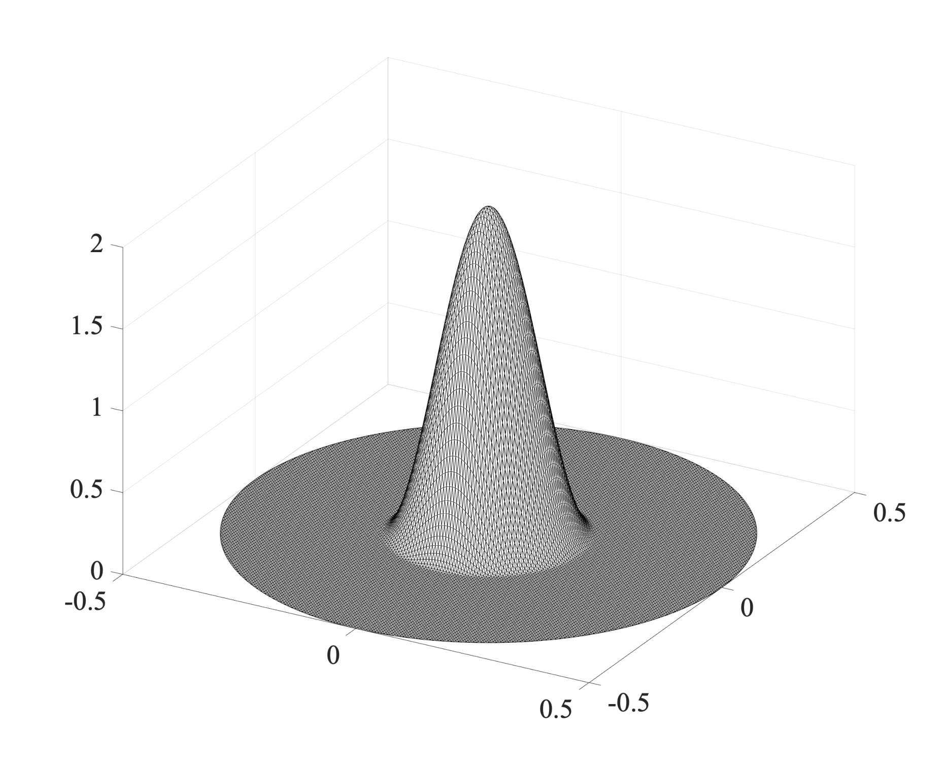
In this example we show the effect of a pulse approaching the boundary for zero Dirichlet boundary conditions and for zero Neumann boundary conditions. The domain is the same as in the previous example, we set $h=7\times 10^{-3}$ , $k=3.93\times 10^{-4}$ . The initial solution is given by

u(r,0)=1+\cos(\pi r/r_{0})\;\;\text{if $r<r_{0}$},u(r,0)=0\;\;\text{elsewhere, and}\;\partial_{t}u=0

(4.3)

with $r_{0}=0.2$ . An interpolated initial condition on the computational mesh is shown in Figure 3. In Figure 4 we show the Dirichlet solution after $t=0.35$ and $t=0.4$ , and in Figure 5 we show the Neumann solution at the same times. The method can clearly handle both hard and soft boundary conditions without modification.

4.3 Increasing Frequency

Here we show the effect of a pulse with decreasing support approaching the boundary. Our domain is $(-0.81,0.79)\times(-0.8,0.8)$ and has Neumann boundary conditions on the uncut boundaries $y=\pm 0.8$ . On the uncut boundary $x=-0.81$ we impose Dirichlet conditions strongly, and on the cut boundary at $x=0.79$ we impose zero Dirichlet boundary conditions weakly. In Fig. 6 we show how the mesh is cut in a closeup. We set $h=8.9\times 10^{-3}$ , $k=3.93\times 10^{-4}$ . The initial solution is given by

u(x,y)=(1+\cos(\pi|x+0.01|/d_{0})\;\;\text{if $|x+0.01|<d_{0}$},u(x,y)=0\;\;\text{elsewhere}

(4.4)

and $\partial_{t}u=0$ , with different $d_{0}$ . This pulse splits into two, one going left and hitting the uncut boundary, one going right and hitting the cut boundary. We show snapshots of the solutions different times and for different $d_{0}$ in Figs. 7–15. Note the dispersion error which becomes more pronounced as $d_{0}$ decreases. The difference in quality of the solution at the uncut and cut boundaries boundary is small and does not become more pronounced as the support of the pulse decreases. We note that as the frequency increases, the meshsize must (eventually) be decreased to avoid dispersion errors, which means the weak Dirichlet data will also be resolved better.

Acknowledgements.

This research was supported in part by the Swedish Foundation for Strategic Research Grant No. AM13-0029, the Swedish Research Council Grants Nos. 2013-4708, 2017-03911, and the Swedish Research Programme Essence. EB was supported in part by the EPSRC grant EP/P01576X/1.

References

[1] S. Badia, F. Verdugo, and A. F. Martín. The aggregated unfitted finite element method for elliptic problems. Comput. Methods Appl. Mech. Engrg., 336:533–553, 2018.
[2] G. A. Baker. Error estimates for finite element methods for second order hyperbolic equations. SIAM J. Numer. Anal., 13(4):564–576, 1976.
[3] G. A. Baker and V. A. Dougalis. The effect of quadrature errors on finite element approximations for second order hyperbolic equations. SIAM J. Numer. Anal., 13(4):577–598, 1976.
[4] E. Burman. Ghost penalty. C. R. Math. Acad. Sci. Paris, 348(21-22):1217–1220, 2010.
[5] E. Burman, S. Claus, P. Hansbo, M. G. Larson, and A. Massing. CutFEM: discretizing geometry and partial differential equations. Internat. J. Numer. Methods Engrg., 104(7):472–501, 2015.
[6] E. Burman and A. Ern. Continuous interior penalty $hp$ -finite element methods for advection and advection-diffusion equations. Math. Comp., 76(259):1119–1140, 2007.
[7] E. Burman and P. Hansbo. Fictitious domain finite element methods using cut elements: II. A stabilized Nitsche method. Appl. Numer. Math., 62(4):328–341, 2012.
[8] P. Clément. Approximation by finite element functions using local regularization. Rev. Française Automat. Informat. Recherche Opérationnelle Sér., 9(R-2):77–84, 1975.
[9] J. Diaz and M. J. Grote. Energy conserving explicit local time stepping for second-order wave equations. SIAM J. Sci. Comput., 31(3):1985–2014, 2009.
[10] M. Drolia, M. S. Mohamed, O. Laghrouche, M. Seaid, and A. El Kacimi. Explicit time integration with lumped mass matrix for enriched finite elements solution of time domain wave problems. Appl. Math. Model., 77(part 2):1273–1293, 2020.
[11] T. Dupont. $L^{2}$ -estimates for Galerkin methods for second order hyperbolic equations. SIAM J. Numer. Anal., 10:880–889, 1973.
[12] M. J. Grote, A. Schneebeli, and D. Schötzau. Discontinuous Galerkin finite element method for the wave equation. SIAM J. Numer. Anal., 44(6):2408–2431, 2006.
[13] M. J. Grote and D. Schötzau. Optimal error estimates for the fully discrete interior penalty DG method for the wave equation. J. Sci. Comput., 40(1-3):257–272, 2009.
[14] P. Hansbo, M. G. Larson, and K. Larsson. Cut finite element methods for linear elasticity problems. In Geometrically unfitted finite element methods and applications, volume 121 of Lect. Notes Comput. Sci. Eng., pages 25–63. Springer, Cham, 2017.
[15] G. M. Hulbert and T. J. R. Hughes. Space-time finite element methods for second-order hyperbolic equations. Comput. Methods Appl. Mech. Engrg., 84(3):327–348, 1990.
[16] A. Johansson and M. G. Larson. A high order discontinuous Galerkin Nitsche method for elliptic problems with fictitious boundary. Numer. Math., 123(4):607–628, 2013.
[17] C. Johnson. Discontinuous Galerkin finite element methods for second order hyperbolic problems. Comput. Methods Appl. Mech. Engrg., 107(1-2):117–129, 1993.
[18] A. Massing, M. G. Larson, A. Logg, and M. E. Rognes. A stabilized Nitsche fictitious domain method for the Stokes problem. J. Sci. Comput., 61(3):604–628, 2014.
[19] L. R. Scott and S. Zhang. Finite element interpolation of nonsmooth functions satisfying boundary conditions. Math. Comp., 54(190):483–493, 1990.
[20] E. M. Stein. Singular integrals and differentiability properties of functions. Princeton Mathematical Series, No. 30. Princeton University Press, Princeton, N.J., 1970.
[21] S. Sticko and G. Kreiss. Higher order cut finite elements for the wave equation. J. Sci. Comput., 80(3):1867–1887, 2019.
[22] S. Sticko, G. Ludvigsson, and G. Kreiss. High-order cut finite elements for the elastic wave equation. Adv. Comput. Math., 46(3):Paper No. 45, 28, 2020.

Authors’ addresses:

Erik Burman, Mathematics, University College London, UK
e.burman@ucl.ac.uk

Peter Hansbo, Mechanical Engineering, Jönköping University, Sweden
peter.hansbo@ju.se

Mats G. Larson, Mathematics and Mathematical Statistics, Umeå University, Sweden
mats.larson@umu.se

Refer to caption — Figure 1: Elevation of the computed solution on a particular mesh.

Figure 2: Convergence at time

T=1

. Dashed line has inclination 1:1, dotted line has inclination

2:1

$\displaystyle\\|E_{h}v\\|_{\mathcal{T}_{h}}$	$\displaystyle=\\|A_{h}F_{h}v\\|_{\mathcal{T}_{h}}$	(2.29)
	$\displaystyle\leq\\|F_{h}v\\|_{\mathcal{T}_{h}}+\\|(I-A_{h})F_{h}v\\|_{\mathcal{T}_{h}}$	(2.30)
	$\displaystyle\lesssim\\|F_{h}v\\|_{\mathcal{T}_{h}}+h^{1/2}\\|[F_{h}v]\\|_{\mathcal{F}_{h}}$	(2.31)
	$\displaystyle\lesssim\\|F_{h}v\\|_{\mathcal{T}_{h}}+\\|F_{h}v\\|_{\mathcal{T}_{h}}$	(2.32)
	$\displaystyle\lesssim\\|v\\|_{\mathcal{T}_{h,I}}$	(2.33)

$\displaystyle\\|\nabla E_{h}v\\|_{\mathcal{T}_{h}}$	$\displaystyle=\\|\nabla A_{h}F_{h}v\\|_{\mathcal{T}_{h}}$	(2.34)
	$\displaystyle\leq\\|\nabla F_{h}v\\|_{\mathcal{T}_{h}}+\\|\nabla(I-A_{h})F_{h}v)\\|_{\mathcal{T}_{h}}$	(2.35)
	$\displaystyle\leq\\|\nabla F_{h}v\\|_{\mathcal{T}_{h}}+h^{-1}\\|(I-A_{h})F_{h}v\\|_{\mathcal{T}_{h}}$	(2.36)
	$\displaystyle\lesssim\\|\nabla F_{h}v\\|_{\mathcal{T}_{h}}+h^{-1/2}\\|[F_{h}v]\\|_{\mathcal{F}_{h}}$	(2.37)
	$\displaystyle\lesssim\\|\nabla v\\|_{\mathcal{T}_{h,I}}$	(2.38)

$\displaystyle\\|(I-A_{h})F_{h}(\pi_{h}Ev)_{I}\\|_{H^{m}(\mathcal{T}_{h})}$	$\displaystyle\lesssim h^{-m}\\|(I-A_{h})F_{h}(\pi_{h}Ev)_{I}\\|_{\mathcal{T}_{h}}$	(2.58)
	$\displaystyle\lesssim h^{1/2-m}\\|[F_{h}(\pi_{h}Ev)_{I}]\\|_{\mathcal{F}_{h}}$	(2.59)
	$\displaystyle\lesssim h^{1/2-m}\\|[F_{h}(\pi_{h}Ev)_{I}-\pi_{h}Ev]\\|_{\mathcal{F}_{h}}$	(2.60)
	$\displaystyle\lesssim h^{-m}\\|F_{h}(\pi_{h}Ev)_{I}-\pi_{h}Ev\\|_{\mathcal{T}_{h}}$	(2.61)
	$\displaystyle\lesssim h^{-m}\\|F_{h}(\pi_{h}Ev)_{I}-P_{h}v\\|_{\mathcal{T}_{h}}+h^{-m}\\|P_{h}v-\pi_{h}Ev\\|_{\mathcal{T}_{h}}$	(2.62)

	$\displaystyle\\|\nabla^{m}(v-R_{h}v)\\|$	$\displaystyle\leq\\|\nabla^{m}(v-I_{h}v)\\|+\\|\nabla^{m}(I_{h}v-{\color[rgb]{0,0,0}R_{h}}v)\\|$		(3.15)
		$\displaystyle\lesssim h^{2-m}\\|v\\|_{H^{2}(\Omega)}+\\|\nabla^{m}(I_{h}v-{\color[rgb]{0,0,0}R_{h}}v)\\|$		(3.16)

	$\displaystyle k^{2}\\|\partial_{t}v^{N-1}\\|_{a_{h}}^{2}+2a_{h}(v^{N-1},v^{N})$	$\displaystyle=\\|v^{N}\\|^{2}_{a_{h}}+\\|v^{N-1}\\|^{2}_{a_{h}}$		(3.57)
	$\displaystyle k^{2}\\|\partial_{t}v^{0}\\|_{a_{h}}^{2}+2a_{h}(v^{0},v^{1})$	$\displaystyle=\\|v^{1}\\|^{2}_{a_{h}}+\\|v^{0}\\|^{2}_{a_{h}}$		(3.58)