Cosmology dependency of halo masses and concentrations in hydrodynamic simulations2020Cosmology dependency of halo masses and concentrations in hydrodynamic simulations–C
Abstract
We employ a set of Magneticum cosmological hydrodynamic simulations that span over different cosmologies, and extract masses and concentrations of all well-resolved haloes between for critical over-densities and mean overdensity We provide the first mass-concentration (Mc) relation and sparsity relation (i.e. mass conversion) of hydrodynamic simulations that is modelled by mass, redshift and cosmological parameters as a tool for observational studies. We also quantify the impact that the Mc relation scatter and the assumption of NFW density profiles have on the uncertainty of the sparsity relation. We find that converting masses with the aid of a Mc relation carries an additional fractional scatter () originated from deviations from the assumed NFW density profile. For this reason we provide a direct mass-mass conversion relation fit that depends on redshift and cosmological parameters. We release the package hydro_mc, a python tool that perform all kind of conversions presented in this paper.
Keywords:
halo - large-scale structure of Universe - cosmological parameters1 Introduction
Early studies of numerical N-body simulations of cosmic structures embedded in cosmological volumes (Navarro et al. 1997; Kravtsov et al. 1997, see e.g.) showed that dark matter haloes can be described by the so called Navarro-Frank-White (NFW) profile (Navarro et al. 1996). The NFW density profile is modelled by a characteristic density and a scale radius in the following way:
| (1) |
The NFW profile proved to match density profiles of dark matter haloes of dark-matter-only (DMO) simulations (Bullock et al. 2001; Suto 2003; Prada et al. 2012; Meneghetti et al. 2014; Klypin et al. 2016; Gupta et al. 2017; Brainerd 2019, see e.g.) up to the largest and most resolved ones whose analyses trace the route for the next generation of (pre-)Exascale simulations. However, density profiles of hydrodynamic simulations have small deviations from the NFW profile (Balmès et al. 2014; Tollet et al. 2016, see e.g.).
Since this kind of density profile does not have a cut-off radius, the radius of a halo is often chosen as the virial radius (Ghigna et al. 1998; Frenk et al. 1999, see e.g.), namely, the radius at which the mean density crosses the one of a theoretical virialised homogeneous top-hat overdensity. Bryan & Norman 1998 showed that the virial overdensity can be written as
| (2) |
where is the scale factor and is the energy density parameter (see Dodelson 2003, for a review), namely
| (3) |
where and are the density fractions of the total matter, radiation, curvature and cosmological constant, respectively. Numerical cosmological simulations, as in this work, typically use negligible radiation and curvature terms (they set in Eq. 3).
Observational studies typically define galaxy cluster (GC) radii as where is an arbitrary overdensity and the "" suffix indicates that the overdensity is relative to the critical overdensity given by,
| (4) |
X-ray observations typically use overdensities and and the corresponding radii and (Bocquet et al. 2019; Umetsu et al. 2019; Mantz 2019; Bulbul et al. 2019, see e.g.), whereas, observational studies that compute dynamical masses typically use (Biviano et al. 2017; Capasso et al. 2019, see e.g.). Weak Lensing studies on the other hand often utilise radii whose overdensities are proportional to the mean density of the Universe. For instance, works such as Mandelbaum et al. 2008; McClintock et al. 2019 measure halo radii as where the suffix "" means that the radius is defined so the mean density of the halo in Eq. 4 crosses (in this case ) where is the average matter density of the Universe.
The concentration of a halo is defined as, , where, is the scale radius of Eq. 1 and quantifies how large the internal region of the cluster is compared to its radius for a given overdensity (see Okoli 2017, for a review). Both numerical and observational studies analyse the concentration of haloes in the context of the so called mass-concentration (Mc) plane (see Table 4 in Ragagnin et al. 2019, for comprehensive list of recent studies). Within the context of hydrodynamic simulations, one can define the DM mass-concentration plane which can be used by observations that estimate DM profiles (Merten et al. 2015, e.g.). On the other hand observations that have only information on the total-matter profile must rely on total-matter mass concentration planes (Raghunathan et al. 2019, e.g).
In search of a realistic estimate of halo concentrations, one must consider the various sources that affect this value. The parameter in both observational and numerical studies is found to have a weak dependence on halo mass and a very large scatter (Bullock et al. 2001; Martinsson et al. 2013; Ludlow et al. 2014; Shan et al. 2017; Shirasaki et al. 2018; Ragagnin et al. 2019). Concentration has been found to depend on a number of factors, as formation time of haloes (Bullock et al. 2001; Rey et al. 2018), accretion histories (Ludlow et al. 2013; Fujita et al. 2018a; Fujita et al. 2018b, see e.g.), dynamical state (Ludlow et al. 2012), triaxiality (Giocoli et al. 2012; Giocoli et al. 2014), and halo environment (Corsini et al. 2018; Klypin et al. 2016). The fractional scatter in the Mc plane is larger than (Heitmann et al. 2016), and observations found outliers with extremely high concentration (Buote & Barth 2019) or very low concentration (Andreon et al. 2019). When all major physical phenomena of galaxy formation are taken into account (cooling, star formation, black hole seeding and their feedback), then concentration parameters are lower than their dark-matter-only counterpart (Wang et al. 2015; Tollet et al. 2016, see e.g. results from NIHAO simulations as in).
Halo concentration parameters are also affected by the underlying cosmological model (see e.g. Roos 2003, for a review on cosmological models). The derived Mc relation is found in fact different in Cold Dark Matter (CDM), CDM, DM, and varying dark energy equation of state (Kravtsov et al. 1997; Ludlow et al. 2016; Dolag et al. 2004; De Boni 2013; De Boni et al. 2013). In general, the Mc dependency of DMO simulations on cosmological parameters has been extensively studied in works as the Cosmic Emulator (Macciò et al. 2008; Bhattacharya et al. 2013; Heitmann et al. 2016), works as Ludlow et al. 2014 and Prada et al. 2012.
Mass-concentration relations allow observational works to convert masses between overdensities. For this purpose, Balmès et al. 2014 defined the sparsity parameter as the ratio between masses at over-density and . This quantity is a proxy to the total matter profile (Corasaniti et al. 2018) and enables cosmological parameter inference (Corasaniti & Rasera 2019) and testing for some dark energy models without assuming an NFW profile (Balmès et al. 2014). Observations use the sparsity parameter to infer the halo matter profile (Bartalucci et al. 2019), as a potential probe to test models (Achitouv et al. 2016), a less uncertain measurement of the mass-concentration relation (Fujita et al. 2019), and to find outliers in scaling relations involving integrated quantities with different radial dependencies (Andreon et al. 2019, see conclusions in).
In this work we use data from the Magneticum suite of simulations (Biffi et al. 2013; Saro et al. 2014; Steinborn et al. 2015; Teklu et al. 2015; Dolag et al. 2015; Dolag et al. 2016; Steinborn et al. 2016; Bocquet et al. 2016; Remus et al. 2017, presented in works such as) to calibrate the cosmology dependence of the mass-concentration and of the mass-sparsity relation of the total matter component from hydrodynamic simulations with the purpose of facilitating cluster-cosmology oriented studies. These studies typically calibrate the observable-mass relation from stacked weak lensing signal under the assumption that mass-calibration can be correctly recovered from DMO Mc relations (e.g. Rozo et al. 2014; Dietrich et al. 2014; Baxter et al. 2016; Simet et al. 2017; Geach & Peacock 2017; McClintock et al. 2019; Raghunathan et al. 2019 and references therein), an approximation that has to be quantified by calibrating the total-mass mass-concentration relations within hydrodynamic simulations (McClintock et al. 2019, see discussion in Sec. 5.4.1 of).
This work represents a first necessary step in this direction and it provides mass-concentration and mass-mass relations that depends on cosmology and that simultaneously accounts for the presence of baryons. While in fact previous works in the literature studied either the dependency of the concentration on cosmological parameters or on baryon physics, in this analysis we calibrate for the first time the dependency of concentration on cosmological parameters in the context of hydrodynamic simulations that include a full description of the main baryonic physical processes.
In Section 2 we present the numerical set up of the simulations used in this work. In Section 3 we fit the concentration of haloes as a function of mass and scale factor for all our simulations and compare our results with both observations and other theoretical studies. In Section 4 we provide a fit of the concentration as a function of mass, scale factor and cosmology. As uncertainty propagation is a delicate and important matter for cluster cosmology experiments, in Sec. 5 we test sparsity parameter and study the origin of its large uncertainty. In order to facilitate cluster cosmology studies that include mass-observable relations which are calibrated at different radii (Bocquet et al. 2016; Bocquet et al. 2019; Mantz 2019; Costanzi et al. 2019, e.g.), we study how to convert masses at different overdensities (the sparsity-mass relation). We summarise our findings, including a careful characterisation of the associated intrinsic scatter. in Sec. 5. We draw our conclusions in Section 7.
2 Numerical Simulations
| Name | |||||||
|---|---|---|---|---|---|---|---|
| (all snapshots) | (snapshot ) | ||||||
| C1 | 0.153 | 0.0408 | 0.614 | 0.666 | 29206 | 9153 | |
| C1_norad | 0.153 | 0.0408 | 0.614 | 0.666 | 27613 | 9208 | |
| C2 | 0.189 | 0.0455 | 0.697 | 0.703 | 54094 | 16236 | |
| C3 | 0.200 | 0.0415 | 0.850 | 0.730 | 107423 | 27225 | |
| C4 | 0.204 | 0.0437 | 0.739 | 0.689 | 66351 | 19051 | |
| C5 | 0.222 | 0.0421 | 0.793 | 0.676 | 84087 | 22037 | |
| C6 | 0.232 | 0.0413 | 0.687 | 0.670 | 47045 | 14930 | |
| C7 | 0.268 | 0.0449 | 0.721 | 0.699 | 58815 | 17990 | |
| C8 | 0.272 | 0.0456 | 0.809 | 0.704 | 79417 | 22353 | |
| C9 | 0.301 | 0.0460 | 0.824 | 0.707 | 96151 | 26473 | |
| C10 | 0.304 | 0.0504 | 0.886 | 0.740 | 120617 | 32551 | |
| C11 | 0.342 | 0.0462 | 0.834 | 0.708 | 97392 | 27100 | |
| C12 | 0.363 | 0.0490 | 0.884 | 0.729 | 118342 | 33571 | |
| C13 | 0.400 | 0.0485 | 0.650 | 0.675 | 35503 | 14626 | |
| C14 | 0.406 | 0.0466 | 0.867 | 0.712 | 104266 | 30918 | |
| C15 | 0.428 | 0.0492 | 0.830 | 0.732 | 92352 | 28348 | |
| C15_norad | 0.428 | 0.0492 | 0.830 | 0.732 | 79399 | 25270 |
Magneticum simulations are performed with an extended version of the Nbody/SPH code P-Gadget3, which is the successor of the code P-Gadget2 (Springel et al. 2005b; Springel 2005; Boylan-Kolchin et al. 2009), with a space-filling curve aware neighbour search (Ragagnin et al. 2016), an improved Smoothed Particle Hydrodynamics (SPH) solver (Beck et al. 2016); treatment of radiative cooling, heating, ultraviolet (UV) background, star formation and stellar feedback processes as in Springel et al. 2005a connected to a detailed chemical evolution and enrichment model as in Tornatore et al. 2007, which follows 11 chemical elements (H, He, C, N, O, Ne, Mg, Si, S, Ca, Fe) with the aid of CLOUDY photo-ionisation code (Ferland et al. 1998). Fabjan et al. 2010; Hirschmann et al. 2014 describe prescriptions for black hole growth and for feedback from AGNs.
Haloes are identified using the version of SUBFIND (Springel et al. 2001), adapted by Dolag et al. 2009 to take the baryon component into account.
Magneticum sub-grid physics does reproduce realistic haloes11 1 In particular, Magneticum simulations match observations of angular momentum for different morphologies (Teklu et al. 2015; Teklu et al. 2016); the mass-size relation (Remus & Dolag 2016; Remus et al. 2017; van de Sande et al. 2019); the dark matter fraction (Remus et al. 2017, see Figure 3 in); the baryon conversion efficiency (Steinborn et al. 2015, see Figure 10 in); kinematical observations of early-type galaxies (Schulze et al. 2018); the inner slope of the total matter density profile (Bellstedt et al. 2018, see Figure 7 in), the ellipticity and velocity over velocity dispersion ratio (van de Sande et al. 2019); and reproduce the high concentration of high luminosity gap of fossil objects (Ragagnin et al. 2019)., thus one can assume that its concentration parameter are realistic and of general applicability for purposes of calibration on observational studies.
Table 1 gives an overview of the cosmological simulations used in this work. They have already been presented in Singh et al. 2019 (see Table 1 in their paper) and labelled as C1–15. Each simulation covers a volume of gas and DM particle masses respectively equal to and and a softening in units of comoving kiloparsec. They have different cosmological parameters and exception for two simulations with the same setup as C1 and C15 (C1_norad and C15_norad) that have been run without radiative cooling and star formation.
For each simulation we study the haloes at a timeslice with redshifts and In the following sections we repeat the same analyses for overdensities performing a corresponding mass-cut (respectively on ) that ensures that all haloes have at least particles. This cut is different for each of our simulations. This is opposed to what was used in Singh et al. 2019, where they choose a fixed mass cut for all C1-C15 simulations. The mass range of these haloes is between , which fits the typical range of galaxy cluster weak-lensing masses (Applegate et al. 2014, see e.g.).
In this work we fit the NFW profile (see Eq. 1) over the total matter component (i.e. dark matter and baryons) as opposed to previous works (Ragagnin et al. 2019, see) where the NFW profile fit was performed over the dark matter component only. We fit the density profile over logarithmic bins, starting from (Dietrich et al. 2019, similar to the cut applied in observational studies as). All fits with a have been excluded from our analyses (which accounts for a few hundred haloes per snapshot) as they correspond to heavily perturbed objects.
Although works on simulations typically present quantities in comoving units of (e.g. distances in ), unless specified, all quantities expressed in this work are in physical units and are not in units of
3 Halo concentrations
In Appendix A we study the effect of baryons on mass-concentration planes and show how an incorrect treatment of baryons can lead to under-estimation of the concentration up to and how the interplay between dark matter and baryons put the dynamical state of hydrodynamic simulations in a much more complex picture than the one of DMO simulations.
This motivates us to study halo masses and concentrations on hydrodynamic simulations, and in particular we focus on their dependency on cosmological parameters. We perform a fit of the concentration as a function of mass and redshift for each simulation at each over-density of Magneticum simulations. The functional form of the concentration is chosen as a power law on mass and scale factor as done in the observational studies (Merten et al. 2015, see e.g.) as:
| (5) |
Here are fit parameters, are median of mass and scale factor, respectively and are used as pivot values, and the fit will be performed including a logarithmic scatter .
We maximised the following likelihood 22 2 we used the python package emcee (Foreman-Mackey et al. 2013) with a uniform prior for all fit parameters:
| (6) |

Figure 1 shows the mass concentration planes for (computed following Eq. 2) for all simulations, together with the concentration from the redshift-mass-concentration (aMc relation) colour coded by . Haloes with high tend to have lower concentration which qualitatively agrees with other theoretical studies that show how perturbed objects have lower concentrations (Balmès et al. 2014; Ludlow et al. 2014; Klypin et al. 2016, see e.g.). For this reason, in a mass-concentration plane, it is not advisable to weight halo concentrations with , as this would bias the relation towards higher concentrations. Although the concentration is believed to decrease with increasing halo mass, extreme cosmologies such as C1 and C2 (with ) have an overall positive dependency between the mass and concentration. On the other hand, the logarithmic mean slope is low (between and ) and its influence in the mass concentration plane is not dominant in our mass regime of interest.
3.1 Comparison with other studies
We then compare Magneticum simulations concentrations of haloes with the concentration predicted by the Cosmic Emulator (Heitmann et al. 2016; Bhattacharya et al. 2013). The Cosmic Emulator is a tool to predict the mass-concentration planes for a given CDM. We were able to compare only C7, C8 and C9 cosmologies because the other Magneticum simulations had cosmological parameters that were out of the range of the Cosmic Emulator. Note that while the Cosmic Emulator dependency on is encoded in the power spectrum normalisation, our mass-concentration relation dependency on takes into account all physical processes of baryon physics, including star formation and feedback.
The ratio of median concentration parameters of haloes obtained with our mass-concentration fit and the concentration provided by the Cosmic Emulator is We notice how the Cosmic Emulator concentrations (retrieved by dark matter only runs) are systematically higher than Magneticum simulations in this mass regime (by a factor of ), in agreement with our comparison in Ragagnin et al. 2019. The scatter is constant over mass, redshift and cosmology, to nearly in agreement with the value of presented in the CDM dark-matter only model of Kwan et al. 2013.

Figure 2 shows the mass-concentration plane for the full-physics simulations C1–15 against other dark matter only simulations and observations. We compare with the concentration from Omega500 simulations (Shirasaki et al. 2018); CLASH concentrations from Merten et al. 2015, numerical predictions from MUSIC of CLASH (Meneghetti et al. 2014), where a number of simulated haloes have been chosen to make mock CLASH observations. To highlight the high scatter in the mass-concentration relation, we also show high concentration groups from Pratt et al. 2016 and an under-luminous and low-concentration halo studied in Andreon et al. 2019. When analysing this data one must be aware of their selection effects: CLASH data-set underwent some filtering difficult to model, while fossil objects presented in Pratt et al. 2016 by construction lay in the upper part of the Mc plane. There is a general agreement between concentration of Magneticum simulations and these observations.
4 Cosmology dependence of concentration parameter
The 15 cosmologies we use in this work have different mass-concentration normalisation values and log-slope (see Figure 1). we perform a fit of the concentration as a function of mass, scale factor and cosmological parameters in order to interpolate a mass-concentration plane at a given, arbitrary, cosmology, i.e. a concentration . As the intrinsic scatter is constant (within few percents) we didn’t further parametrise it and assumed it to be independent of mass, redshift and cosmology. The functional form of the fit parameters in Eq. 5, with a dependency on cosmology is as follows:
| (7) |
| Param | Overdensity | ||||
|---|---|---|---|---|---|
| vir | 200c | 500c | 2500c | 200m | |
The fit has been performed for and by maximising the Likelihood as in Eq 6. Table 2 shows the results with cosmological parameter pivots at the reference cosmology C8.
Given the high number of free parameters, in order to not underestimate possible sources of errors in the fit, we decided to evaluated uncertainties as follows in Singh et al. 2019: (1) we first re-performed the fit for each simulation by setting its own cosmological parameter as pivot values; (2) then for each parameter except we considered the standard deviation of the parameter values in the previous fits and set it as uncertainty in Table 2; (3) parameters are presented without uncertainty because the error obtained from the Hessian matrix is negligible compared to the scatter parameter Being this work first necessary step towards a cosmology-dependent mass-concentration relation, these parameters may be constrained with more precision in future simulation campaigns.
From the above fit we find that the normalisation ( parameters) is mainly affected by and . The slope of the mass-concentration plane ( parameters) has a weak dependency on cosmology. However, the logarithmic mass slope is pushed towards negative values by an increase in and (i.e. and ), while it is pushed towards positive values by an increase in and (since and ). This behaviour is also shown in Figure 2. Note that, C1 and C2 have opposite mass-dependency with respect to the other runs. Although the trend can be positive for some cosmologies (see Table 2 and Figure 1), the slope is always close to zero. The redshift dependency ( parameters) is driven by both and while a high baryon fraction can lower the dependency (see parameter ). The scatter is nearly constant for all the overdensities with a value close to and even if it is of the same order of the difference between Mc relations of different cosmologies (see shaded area in Fig. 2), in the next sub-section we will show that statistical studies on large samples of galaxy clusters are still affected by the cosmological dependency of Mc relations.
Since the logarithmic slope of the mass has a weak dependency on cosmology, we provide a similar fit as the one in this section without having any cosmological dependencies i.e. in Appendix B (see Table 5). In Appendix B (see Table 6) we also provide the same reduced fit parameters with the scale radius computed on the dark matter density profile.
4.1 Impact on inferred weak-lensing masses


There are differences between the Mc relation extracted from our simulations at different cosmologies and the ones from DMO simulations. When Mc relations are used to provide priors and interpret the weak-lensing signal of non-ideal NFW cluster samples, the different Mc relations will ultimately lead to different inferred masses and therefore different cosmological constraints from cluster number counts experiments. In fact, works as Henson et al. 2017 show that it is possible to correctly recover halo masses from mock observations of both DMO and hydro-simulations by using their respective mass-concentration relations. On the other hand, in low signal-to-noise conditions, weak-lensing mass calibration typically constrains the total observed mass using Mc relations derived from DMO simulations (Melchior et al. 2017, see, e.g., ). In the following, we quantify and discuss this effect on a simplified example.
To this end, we create a simulated projected surface density profile of an NFW model of the RXC J2248.7-4431 cluster (Gruen et al. 2013), at with mass (Melchior et al. 2015). The simulated profile is generated using Eq. 41 in Łokas & Mamon 2001 with a concentration from our Mc relation (see Table 2) and with cosmological parameters . We mimic a simplified observed radial profile sampled with logarithmic equally spaced radial bins from to arcmin. To each data-point we assigned an associated error in order to simulate typical weak-lensing observational conditions () of a massive clusters in a photometric survey like the Dark Energy Survey (Melchior et al. 2015, DES,). We test a simplified mass calibration process by fitting the above described density profile with a gaussian likelihood for each simulated projected density radial bin :
| (8) |
We adopt a flat prior on log and test the impact of adopting the following different priors for the concentration:
- •
Ragagnin20: The Mc relation with a lognormal scatter as presented in this work.
- •
Diemer19: The DMO Mc relation proposed in Diemer & Joyce 201933 3 We used the python package https://bdiemer.bitbucket.io/colossus/ (Diemer 2018, see). with a lognormal scatter .
To show the impact on mass-calibration of Ragagnin20 and the dependency on cosmological parameters, we perform the calibration both at the correct input cosmology (from here on Cosmo A) and with cosmological parameters randomly extracted from the posterior distribution of the cosmological parameters derived by SPT cluster number counts (Bocquet et al. 2019, from here on Cosmo B).
Figure 3 (top panel) shows the ideal un-perturbed mock profile and best fit realisations of NFW profiles produced using Ragagnin20 (red line) and Diemer19 (blue line). The Mc relation presented in this work has a lower concentration normalisation than Diemer19 (Appendix A), and thus Ragagnin20 produce lower values of surface densities near the centre and higher values on the outskirts with respect to DMO mass-concentration relations. Different prior assumptions on the Mc relation affect the inferred mass, as we see in Figure 3 (middle panel)44 4 Parameter space is sampled with emcee.. While the posterior derived assuming the Mc relations of Ragagnin20 and of Diemer19 are in good agreement, the best fit mass recovered with Diemer19 is higher compared to the one derived with Ragagnin20. This can be better appreciated in the bottom panel of Figure 3, where we instead simulate the mass calibration of a stack of clusters (Melchior et al. 2017). We therefore mimic a stacked average profile and decrease by a factor of the intrinsic scatter around the Mc relation in the prior. Assuming the wrong Cosmo B cosmology, we would recover biased results using both the Ragagnin20 and the Diemer19 Mc relation, even if the marginalized posterior on the mass would be almost unbiased for the Ragagnin20 analysis. Furthermore we note that fixing Cosmo B cosmolgy instead of the correct input Cosmo A cosmolgy would result in a slightly smaller mass for Ragagnin20 and in a slightly larger mass for Diemer19. While a more sophisticated analysis including a treatment of systematic uncertainties and a self-consistent exploration of the cosmological parameters is beyond the purpose of this work, this simple exercise highlights the importance of a correct modelization of the cosmological dependence of the Mc relation in the the weak-lensing analysis of cluster samples for cosmological purposes.
We stress that in this experiment we wanted to mimic the procedure of most observational works, thus we didn’t model baryon component of DMO simulations.
5 Halo masses conversion
In the following subsections, we present and compare different methods of converting masses between overdensities. We also provide a direct fit for converting masses (i.e. SUBFIND masses) from to (thus without using the Mc relation), in order to study the origin of the scatter coming from the conversions. This kind of conversions is used in computing the sparsity of haloes (i.e. ratio of masses in two overdensities), which itself can probe cosmological parameters (Corasaniti et al. 2018; Corasaniti & Rasera 2019) and dark energy models (Balmès et al. 2014).
5.1 Mass-mass conversion using Mc relation
In this section, we tackle the problem of converting masses via a Mc relation. By combining the definition of mass (see Eq. 4) and the fact that the matter profile only depends on a proportional parameter and a scale radius we get
| (9) |
For a NFW profile as in Eq. 1,
| (10) |
| (11) |
From the second part of Eq. 11 it is possible to evaluate the concentration as a function of only (Hu & Kravtsov 2003, as in Appendix C of).
Eq. 11 can be used to estimate the theoretical scatter obtained in the mass conversion by analytically propagating the uncertainties of the mass-concentration relation, namely:
| (12) |
where is the converted mass, the concentration in the original overdensity and is the uncertainty in the concentration (in our case it is the scatter in the Mc relation). Appendix C describes how to obtain the theoretical scatter one would expect given a perfectly NFW profile.
There are several sources of error in the mass-mass conversion derived by a mass-concentration relation: (i) the intrinsic scatter of the Mc relation, (ii) the fact that profiles are not perfectly NFW and thus Eq. 10 is not the best choice for this conversion; (iii) the cosmology-redshift-mass-concentration fit (as in Table 2) may not be optimal.
To further study the sources of uncertainties in this conversion, we fit SUBFIND halo masses between two overdensities55 5 The package hydro_mc contains a sample script to convert masses between two overdensities by using the mass-concentration relation presented in this paper (http://github.com/aragagnin/hydro_mc/blob/master/examples/sample_mm_from_mc_relation.py)., and compare the two conversion methods.
5.2 - (M-M) plane
In this subsection we perform a direct fit between halo masses (i.e. SUBFIND masses), as a function of redshift and cosmological parameter. The reason of this fit is twofold: (1) we want to study the uncertainty introduced in the conversion of the previous subsection and (2) we want to provide a way of converting masses without any assumption on their concentration and NFW density profile.
For each pair of overdensities we performed a fit of the mass with the following functional form:
| (13) |
where parameters are parametrised with cosmology as in Eq. 7.
| Param | From overdensity to overdensity | |||||
|---|---|---|---|---|---|---|
| Param | From overdensity to overdensity | |||||
|---|---|---|---|---|---|---|
| Param | From overdensity to overdensity | |
|---|---|---|
5.3 Uncertainties in mass conversions
When converting between masses at different overdensities, we are interested in the the following sources of uncertainty:
- •
the scatter from the mass-mass conversion obtained with the aid of our Mc relation found in Sec. 5.1.
- •
the scatter obtained from a conversion between the true values of and of a given halo to (i.e. using only Eq. 11). We use this scatter in order to estimate the error coming from non-NFWness (i.e. deviation from perfect NFW density profile).
- •
- •
the scatter that is supposed to be introduced by a non-ideal cosmology-redshift-mass-concentration fitting formula.
- •
In a simplistic approach, the quadrature sum of the scatter coming from non-NFWness ( ), the theoretical scatter () and the scatter due to a non-ideal Mc fit (), should all add up to the scatter in the mass-mass conversion using a mass-concentration relation:
| (14) |
5.4 Obtaining from or
In this subsection we test mass conversion to given or We compare results obtained using the technique described in Sec 5.1 against the mass-mass relation from Eq. 13.
We tested the conversion in the mass regime of and found the following scatter values: and by converting masses using Sec. 5.1 and by using conversion table in Sec. 5.2. We are confident to have all uncertainty sources under control because the quadrature sum of all scatters from conversion described in Sec. 5.2 (i.e. ) equals from Sec. 5.1 as in Eq. 14.
We repeat the same conversion for and find the following scatter values: by converting masses using Sec. 5.1 and by using conversion table in Sec. 5.2. In this conversion, the quadrature sum of the theoretical scatters in Eq. 14 holds only if we attribute an additional source of the uncertainty to a non-ideal - relation fit
This means that a direct mass-mass fit is more precise than a conversion that passes through an Mc relation when converting
It is interesting to see that in both scenarios the conversion with the lowest scatter is the one performed with the exact knowledge of both mass and concentration (i.e. is the lowest). On the other hand, in the scenario where one only knows the mass of a halo, then the conversion with the lowest uncertainty is the one that uses relation in Sec. 5.2 (i.e. with a scatter ).
6 Discussion on cosmology dependency of masses and concentrations

The concentration of haloes at fixed mass is a non trivial function of cosmological parameters. We summarise in Figure 4 (upper panel) the variation of as a function of cosmological parameters for a halo of mass to provide a more intuitive representation. In general concentration normalisation decreases with baryon fraction While a small () decrease is expected also on DMO models as Diemer & Joyce 2019, our change in this mass range is likely associated with feedback from AGN, as an increase of gas fraction implies more energy released by feedback processes, which is known to lower concentration. The logarithmic mass slope of the Mc (see Table 2) increases with , in agreement with SNe feedback being less relevant in massive haloes. For concentration at the situation is less clear. is closer to the centre of the halo and depends more strongly on physical processes which are not solely regulated by gravity. The qualitative behaviour is nevertheless consistent with , with the strongest (positive) cosmological dependence on and , a weak (negative) dependency on , and a weaker one on . It is not possible to infer the effect of on the redshift log-slope as its value is mainly driven by
C1 and C2 simulations show a positive correlation between mass and concentration. This is in agreement with Prada et al. 2012, where they found that haloes with low r.m.s. fluctuation amplitude have a concentration that increases with mass. In fact C1 and C2 have extremely low values of (i.e. ) which leads to low r.m.s. fluctuation amplitudes.
When converting masses from higher overdensities to lower overdensities the scatter increases as the difference between overdensities increases (see Table 3). Figure 4 (lower panel) shows the variation of sparsity normalisation as a function of cosmological parameters. The log-slope of the mass dependency ( parameters) has almost no dependency on cosmology. One exception is made by where normalisation does depend on Note that this relation doesn’t assume any density profile, thus this dependency cannot be caused by a bad NFW fit. This effect is probably due to baryon feedback that at this scale is capable of influencing the total matter density profile.
The redshift dependency ( parameters) is mostly influenced by and with a contribution that increases with separation between overdensities, which may indicates a different growth of the internal and external regions of the halo.
7 Conclusions
We provided mass-concentration relations and mass conversion relations between overdensities that include dependencies on the cosmological parameters without modelling dynamical state of the simulated haloes. We showed that mass calibrated with DMO Mc relation can be higher compared with masses calibrated with our Mc relation. Additionally, cluster-cosmology oriented studies will benefit from this work since this relation averages over all different dynamical states and includes the average effect of baryon physics.
For these reasons we performed the following studies:
- •
- •
We explored the possibility of converting masses between overdensities with and without the aid of our mass-concentration relation and, for the latter, we studied the origin of its uncertainty as being caused by (i) non-NFWness of profiles and (ii) a non-ideal mass-concentration fit. In particular, when converting masses via an Mc relation, non-NFWness of density profiles accounts for approx. of the scatter. Additionally the conversion between to has an additional fractional scatter of caused by the non-ideal mass-concentration relation fit.
- •
In Sec. 6 we discuss the dependency of halo masses and concentration as a function of cosmological parameters. Although concentration is mainly driven by and we found that do decreases concentration and a higher lowers the concentration of the internal part of the halo, probably because of the related scale-dependent baryon feedback. We also found that the positive mass-concentration trend in and is due to their low
We released the python package hydro_mc (github.com/aragagnin/hydro_mc). This tool is able to perform all kinds of conversions presented in this paper and we provided a number of ready-to-use examples: mass-concentration relation presented in Table 2 (http://github.com/aragagnin/hydro_mc/blob/master/examples/sample_mc.py), mass-mass conversion with fit parameters in Table 3 (http://github.com/aragagnin/hydro_mc/blob/master/examples/sample_mm.py), and mass-mass conversion through the Mc relation in Table 2 (http://github.com/aragagnin/hydro_mc/blob/master/examples/sample_mm_from_mc_relation.py).
Acknowledgements
The Magneticum Pathfinder simulations were partially performed at the Leibniz-Rechenzentrum with CPU time assigned to the Project ‘pr86re’. AR is supported by the EuroEXA project (grant no. 754337). KD acknowledges support by DAAD contract number 57396842. AR acknowledges support by MIUR-DAAD contract number 34843 ,,The Universe in a Box”. AS and PS are supported by the ERC-StG ’ClustersXCosmo’ grant agreement 716762. AS is supported by the the FARE-MIUR grant ’ClustersXEuclid’ R165SBKTMA and by INFN InDark Grant. This work was supported by the Deutsche Forschungsgemeinschaft (DFG, German Research Foundation) under Germany’s Excellence Strategy - EXC-2094 - 390783311. We are especially grateful for the support by M. Petkova through the Computational Center for Particle and Astrophysics (C2PAP). Information on the Magneticum Pathfinder project is available at http://www.magneticum.org. We acknowledge the use of Bocquet & Carter 2016 python package to produce the MCMC plots. We thank the referee for the useful comments, which we believe significantly improved the clarity of the manuscript. We also thanks Stefano Andreon for the useful feedback on this paper.
Data Availability
The data underlying this article will be shared on reasonable request to the corresponding author.
References
- Achitouv et al. (2016) Achitouv I., Baldi M., Puchwein E., Weller J., 2016, Phys. Rev. D, 93, 103522
- Andreon et al. (2019) Andreon S., Moretti A., Trinchieri G., Ishwara-Chand ra C. H., 2019, A&A, 630, A78
- Applegate et al. (2014) Applegate D. E., et al., 2014, MNRAS, 439, 48
- Balmès et al. (2014) Balmès I., Rasera Y., Corasaniti P. S., Alimi J. M., 2014, MNRAS, 437, 2328
- Bartalucci et al. (2019) Bartalucci I., Arnaud M., Pratt G. W., Démoclès J., Lovisari L., 2019, A&A, 628, A86
- Baxter et al. (2016) Baxter E., et al., 2016, MNRAS, 461, 4099
- Beck et al. (2016) Beck A. M., et al., 2016, MNRAS, 455, 2110
- Bellstedt et al. (2018) Bellstedt S., et al., 2018, MNRAS, 476, 4543
- Bhattacharya et al. (2013) Bhattacharya S., Habib S., Heitmann K., Vikhlinin A., 2013, ApJ, 766, 32
- Biffi et al. (2013) Biffi V., Dolag K., Böhringer H., 2013, MNRAS, 428, 1395
- Biviano et al. (2017) Biviano A., et al., 2017, A&A, 607, A81
- Bocquet & Carter (2016) Bocquet S., Carter F. W., 2016, The Journal of Open Source Software, 1
- Bocquet et al. (2016) Bocquet S., Saro A., Dolag K., Mohr J. J., 2016, MNRAS, 456, 2361
- Bocquet et al. (2019) Bocquet S., et al., 2019, ApJ, 878, 55
- Boylan-Kolchin et al. (2009) Boylan-Kolchin M., Springel V., White S. D. M., Jenkins A., Lemson G., 2009, MNRAS, 398, 1150
- Brainerd (2019) Brainerd T., 2019, in American Astronomical Society Meeting Abstracts #233. p. 338.06
- Bryan & Norman (1998) Bryan G. L., Norman M. L., 1998, ApJ, 495, 80
- Bulbul et al. (2019) Bulbul E., et al., 2019, ApJ, 871, 50
- Bullock et al. (2001) Bullock J. S., Kolatt T. S., Sigad Y., Somerville R. S., Kravtsov A. V., Klypin A. A., Primack J. R., Dekel A., 2001, MNRAS, 321, 559
- Buote & Barth (2019) Buote D. A., Barth A. J., 2019, ApJ, 877, 91
- Capasso et al. (2019) Capasso R., et al., 2019, arXiv e-prints, p. arXiv:1910.04773
- Chandrasekhar (1961) Chandrasekhar S., 1961, Hydrodynamic and hydromagnetic stability
- Ciesielski (2007) Ciesielski K., 2007, Banach J. Math. Anal., 1, 1
- Corasaniti & Rasera (2019) Corasaniti P. S., Rasera Y., 2019, MNRAS, 487, 4382
- Corasaniti et al. (2018) Corasaniti P. S., Ettori S., Rasera Y., Sereno M., Amodeo S., Breton M. A., Ghirardini V., Eckert D., 2018, ApJ, 862, 40
- Corsini et al. (2018) Corsini E. M., et al., 2018, A&A, 618, A172
- Costanzi et al. (2019) Costanzi M., et al., 2019, MNRAS, 488, 4779
- Cui et al. (2017) Cui W., Power C., Borgani S., Knebe A., Lewis G. F., Murante G., Poole G. B., 2017, MNRAS, 464, 2502
- De Boni (2013) De Boni C., 2013, arXiv e-prints,
- De Boni et al. (2013) De Boni C., Ettori S., Dolag K., Moscardini L., 2013, MNRAS, 428, 2921
- Diemer (2018) Diemer B., 2018, ApJS, 239, 35
- Diemer & Joyce (2019) Diemer B., Joyce M., 2019, ApJ, 871, 168
- Dietrich et al. (2014) Dietrich J. P., et al., 2014, MNRAS, 443, 1713
- Dietrich et al. (2019) Dietrich J. P., et al., 2019, MNRAS, 483, 2871
- Dodelson (2003) Dodelson S., 2003, Modern cosmology
- Dolag et al. (2004) Dolag K., Bartelmann M., Perrotta F., Baccigalupi C., Moscardini L., Meneghetti M., Tormen G., 2004, A&A, 416, 853
- Dolag et al. (2009) Dolag K., Borgani S., Murante G., Springel V., 2009, MNRAS, 399, 497
- Dolag et al. (2015) Dolag K., Gaensler B. M., Beck A. M., Beck M. C., 2015, MNRAS, 451, 4277
- Dolag et al. (2016) Dolag K., Komatsu E., Sunyaev R., 2016, MNRAS, 463, 1797
- Fabjan et al. (2010) Fabjan D., Borgani S., Tornatore L., Saro A., Murante G., Dolag K., 2010, MNRAS, 401, 1670
- Ferland et al. (1998) Ferland G. J., Korista K. T., Verner D. A., Ferguson J. W., Kingdon J. B., Verner E. M., 1998, PASP, 110, 761
- Foreman-Mackey et al. (2013) Foreman-Mackey D., Hogg D. W., Lang D., Goodman J., 2013, PASP, 125, 306
- Frenk et al. (1999) Frenk C. S., et al., 1999, ApJ, 525, 554
- Fujita et al. (2018a) Fujita Y., Umetsu K., Rasia E., Meneghetti M., Donahue M., Medezinski E., Okabe N., Postman M., 2018a, ApJ, 857, 118
- Fujita et al. (2018b) Fujita Y., Umetsu K., Ettori S., Rasia E., Okabe N., Meneghetti M., 2018b, ApJ, 863, 37
- Fujita et al. (2019) Fujita Y., et al., 2019, Galaxies, 7, 8
- Geach & Peacock (2017) Geach J. E., Peacock J. A., 2017, Nature Astronomy, 1, 795
- Ghigna et al. (1998) Ghigna S., Moore B., Governato F., Lake G., Quinn T., Stadel J., 1998, MNRAS, 300, 146
- Giocoli et al. (2012) Giocoli C., Meneghetti M., Ettori S., Moscardini L., 2012, MNRAS, 426, 1558
- Giocoli et al. (2014) Giocoli C., Meneghetti M., Metcalf R. B., Ettori S., Moscardini L., 2014, MNRAS, 440, 1899
- Gruen et al. (2013) Gruen D., et al., 2013, MNRAS, 432, 1455
- Gupta et al. (2017) Gupta N., Saro A., Mohr J. J., Dolag K., Liu J., 2017, MNRAS, 469, 3069
- Heitmann et al. (2016) Heitmann K., et al., 2016, ApJ, 820, 108
- Henson et al. (2017) Henson M. A., Barnes D. J., Kay S. T., McCarthy I. G., Schaye J., 2017, MNRAS, 465, 3361
- Hirschmann et al. (2014) Hirschmann M., Dolag K., Saro A., Bachmann L., Borgani S., Burkert A., 2014, MNRAS, 442, 2304
- Hoekstra et al. (2015) Hoekstra H., Herbonnet R., Muzzin A., Babul A., Mahdavi A., Viola M., Cacciato M., 2015, MNRAS, 449, 685
- Hu & Kravtsov (2003) Hu W., Kravtsov A. V., 2003, ApJ, 584, 702
- Klypin et al. (2016) Klypin A., Yepes G., Gottlöber S., Prada F., Heß S., 2016, MNRAS, 457, 4340
- Komatsu et al. (2009) Komatsu E., et al., 2009, ApJS, 180, 330
- Komatsu et al. (2011) Komatsu E., et al., 2011, ApJS, 192, 18
- Kravtsov et al. (1997) Kravtsov A. V., Klypin A. A., Khokhlov A. M., 1997, ApJS, 111, 73
- Kwan et al. (2013) Kwan J., Bhattacharya S., Heitmann K., Habib S., 2013, ApJ, 768, 123
- Łokas & Mamon (2001) Łokas E. L., Mamon G. A., 2001, MNRAS, 321, 155
- Ludlow et al. (2012) Ludlow A. D., Navarro J. F., Li M., Angulo R. E., Boylan-Kolchin M., Bett P. E., 2012, MNRAS, 427, 1322
- Ludlow et al. (2013) Ludlow A. D., et al., 2013, MNRAS, 432, 1103
- Ludlow et al. (2014) Ludlow A. D., Navarro J. F., Angulo R. E., Boylan-Kolchin M., Springel V., Frenk C., White S. D. M., 2014, MNRAS, 441, 378
- Ludlow et al. (2016) Ludlow A. D., Bose S., Angulo R. E., Wang L., Hellwing W. A., Navarro J. F., Cole S., Frenk C. S., 2016, MNRAS, 460, 1214
- Macciò et al. (2008) Macciò A. V., Dutton A. A., van den Bosch F. C., 2008, MNRAS, 391, 1940
- Mandelbaum et al. (2008) Mandelbaum R., Seljak U., Hirata C. M., 2008, J. Cosmology Astropart. Phys., 8, 006
- Mantz (2019) Mantz A. B., 2019, MNRAS, 485, 4863
- Martinsson et al. (2013) Martinsson T. P. K., Verheijen M. A. W., Westfall K. B., Bershady M. A., Andersen D. R., Swaters R. A., 2013, A&A, 557, A131
- McClintock et al. (2019) McClintock T., et al., 2019, MNRAS, 482, 1352
- Melchior et al. (2015) Melchior P., Sheldon E., Drlica-Wagner A., Rykoff E. S., 2015, DES exposure checker: Dark Energy Survey image quality control crowdsourcer (ascl:1511.017)
- Melchior et al. (2017) Melchior P., et al., 2017, MNRAS, 469, 4899
- Melchior et al. (2018) Melchior P., Moolekamp F., Jerdee M., Armstrong R., Sun A. L., Bosch J., Lupton R., 2018, Astronomy and Computing, 24, 129
- Meneghetti et al. (2014) Meneghetti M., et al., 2014, ApJ, 797, 34
- Merten et al. (2015) Merten J., et al., 2015, ApJ, 806, 4
- Navarro et al. (1996) Navarro J. F., Frenk C. S., White S. D. M., 1996, ApJ, 462, 563
- Navarro et al. (1997) Navarro J. F., Frenk C. S., White S. D. M., 1997, ApJ, 490, 493
- Okabe & Smith (2016) Okabe N., Smith G. P., 2016, MNRAS, 461, 3794
- Okoli (2017) Okoli C., 2017, arXiv e-prints, p. arXiv:1711.05277
- Prada et al. (2012) Prada F., Klypin A. A., Cuesta A. J., Betancort-Rijo J. E., Primack J., 2012, MNRAS, 423, 3018
- Pratt et al. (2016) Pratt G. W., Pointecouteau E., Arnaud M., van der Burg R. F. J., 2016, A&A, 590, L1
- Ragagnin et al. (2016) Ragagnin A., Tchipev N., Bader M., Dolag K., Hammer N. J., 2016, in Advances in Parallel Computing, Volume 27: Parallel Computing: On the Road to Exascale, Edited by Gerhard R. Joubert, Hugh Leather, Mark Parsons, Frans Peters, Mark Sawyer. IOP Ebook, ISBN: 978-1-61499-621-7, pages 411-420. (arXiv:1810.09898), doi:10.3233/978-1-61499-621-7-411
- Ragagnin et al. (2019) Ragagnin A., Dolag K., Moscardini L., Biviano A., D’Onofrio M., 2019, MNRAS, 486, 4001
- Raghunathan et al. (2019) Raghunathan S., et al., 2019, ApJ, 872, 170
- Remus & Dolag (2016) Remus R.-S., Dolag K., 2016, in The Interplay between Local and Global Processes in Galaxies,. p. 43
- Remus et al. (2017) Remus R.-S., Dolag K., Naab T., Burkert A., Hirschmann M., Hoffmann T. L., Johansson P. H., 2017, MNRAS, 464, 3742
- Rey et al. (2018) Rey M. P., Pontzen A., Saintonge A., 2018, arXiv e-prints,
- Roos (2003) Roos M., 2003, Introduction to Cosmology, Third Edition
- Rozo et al. (2014) Rozo E., Bartlett J. G., Evrard A. E., Rykoff E. S., 2014, MNRAS, 438, 78
- Saro et al. (2014) Saro A., et al., 2014, MNRAS, 440, 2610
- Schulze et al. (2018) Schulze F., Remus R.-S., Dolag K., Burkert A., Emsellem E., van de Ven G., 2018, MNRAS, 480, 4636
- Shan et al. (2017) Shan H., et al., 2017, ApJ, 840, 104
- Shirasaki et al. (2018) Shirasaki M., Lau E. T., Nagai D., 2018, MNRAS, 477, 2804
- Simet et al. (2017) Simet M., McClintock T., Mandelbaum R., Rozo E., Rykoff E., Sheldon E., Wechsler R. H., 2017, MNRAS, 466, 3103
- Singh et al. (2019) Singh P., Saro A., Costanzi M., Dolag K., 2019, arXiv e-prints, p. arXiv:1911.05751
- Springel (2005) Springel V., 2005, MNRAS, 364, 1105
- Springel et al. (2001) Springel V., White S. D. M., Tormen G., Kauffmann G., 2001, MNRAS, 328, 726
- Springel et al. (2005a) Springel V., Di Matteo T., Hernquist L., 2005a, MNRAS, 361, 776
- Springel et al. (2005b) Springel V., et al., 2005b, Nature, 435, 629
- Steinborn et al. (2015) Steinborn L. K., Dolag K., Hirschmann M., Prieto M. A., Remus R.-S., 2015, MNRAS, 448, 1504
- Steinborn et al. (2016) Steinborn L. K., Dolag K., Comerford J. M., Hirschmann M., Remus R.-S., Teklu A. F., 2016, MNRAS, 458, 1013
- Suto (2003) Suto Y., 2003, arXiv e-prints, pp astro–ph/0311575
- Teklu et al. (2015) Teklu A. F., Remus R.-S., Dolag K., Beck A. M., Burkert A., Schmidt A. S., Schulze F., Steinborn L. K., 2015, ApJ, 812, 29
- Teklu et al. (2016) Teklu A. F., Remus R.-S., Dolag K., 2016, in The Interplay between Local and Global Processes in Galaxies,. p. 41
- Tollet et al. (2016) Tollet E., et al., 2016, MNRAS, 456, 3542
- Tornatore et al. (2007) Tornatore L., Borgani S., Dolag K., Matteucci F., 2007, Monthly Notices of the Royal Astronomical Society, 382, 1050
- Umetsu et al. (2019) Umetsu K., et al., 2019, arXiv e-prints, p. arXiv:1909.10524
- Wang et al. (2015) Wang L., Dutton A. A., Stinson G. S., Macciò A. V., Penzo C., Kang X., Keller B. W., Wadsley J., 2015, MNRAS, 454, 83
- Zhang et al. (2016) Zhang C., Yu Q., Lu Y., 2016, ApJ, 820, 85
- van de Sande et al. (2019) van de Sande J., et al., 2019, MNRAS, 484, 869
Appendix A Effects of baryons
In this appendix section, we show the importance of correctly describing baryon physics on the estimation of halo concentration. Since all simulations (C1-C15) share the same initial conditions, it is possible to study the evolution of the same halo that evolved differently in different cosmologies.
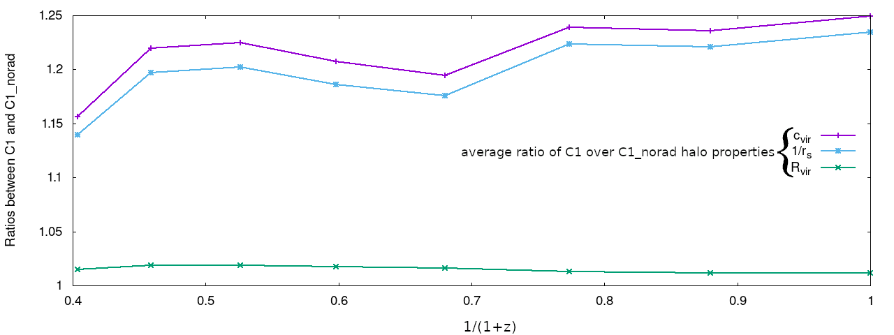

Figure 5 shows the evolution of both the virial radii and scale radii of haloes in C1 and C1_norad. Figure 5 (upper panel) shows the stacked ratio of concentration, virial radius and the scale radius. On an average, C1 haloes have higher concentration parameters ( higher, up to ) and this difference grows with time. Intuitively one may think that the difference in concentration between C1 and C1_norad would be due to a difference in the virial radius. However, the figure shows that it is the scale radius that produce the difference in concentration between the full physics run and the non-radiative one.
Figure 5 (bottom panel) focuses on the evolution of a single halo (bottom left panel shows the evolution of the halo in C1, whereas, the bottom right panel shows the same halo in C1_norad). Simulations without radiative cooling produce haloes with lower concentration with respect to their full physics counterpart (i.e. lowers down to ). This example shows that in non-radiative simulations, concentration decreases even if the full physics counterpart is characterised by the same accretion history (”jumps” in concentration and values happen at the same scale factor).

Dynamical state is known to be related to halo concentrations (Ludlow et al. 2012) and can be quantified using the virial ratio (Cui et al. 2017), , where is the total potential energy, is the total kinetic energy (including gas thermal pressure) and is the energy from surface pressure (from kinetic and thermal energy) at the halo boundary. As described in Chandrasekhar 1961, is gievn by,
| (15) |
Cui et al. 2017 showed that baryonic physics can lower the virial ratio up to w.r.t. DMO runs and Zhang et al. 2016 showed that merger timescale is shortened by a factor of up to 3 for merging clusters with gas fractions , compared to the timescale obtained with no gas.
Figure 6 shows for a DMO run (left panel) and a hydrodynamic run (right panel) that shares the same initial conditions66 6 We use Magneticum/Box0_mr simulation, with size and gravitational softening down to gas and DM mass particles of and respectively, as presented in Bocquet et al. 2016.. The two runs display a different behaviour for highly concentrated objects (): DMO ones have low surface pressure and low total kinetic energy, while hydrodynamic ones show a much more complex and noisy relation between and
It is well known that concentration does depend on dynamical state. Here we also noted how hydrodynamic simulations compared to DMO runs do show even a more noisy and complex relation between concentration and the virial ratio. However, given that the majority of observational studies that investigate large cluster samples lack data to accurately determine their dynamical state (see e.g. studies presented in Hoekstra et al. 2015, Okabe & Smith 2016, Melchior et al. 2018, Dietrich et al. 2019, Mantz 2019, Bocquet et al. 2019 and references therein) they will benefit from a mass-concentration relation built from hydrodynamic simulations that already averages over all possible dynamical states of a halo, as in this work.
The average concentration of haloes shown in Figure 2 are lower than the concentration computed using the dark-matter density profile presented in a previous work on Magneticum simulations (Ragagnin et al. 2019, which uses the same cosmology as C8). The median concentration for cosmology C8 is for the total matter profile, while the dark matter concentration presented in (Ragagnin et al. 2019) has

Such discrepancy is due to the fact that dark matter component is more peaked in the central region with respect to the total matter density. Figure 7 shows an example of the matter density profiles of a Magneticum halo. Here the DM halo has a scale radius of kpc/h while the total matter scale radius is kpc/h: collisional particles and stars formed from them (and their associated heating processes as SN and AGN feedback) are capable of lowering a concentration parameter of .
Appendix B Cosmology-Mass-Redshift-concentration relation lite
Given the weak dependency of mass from the concentration (at least in the mass range of interests of cluster of galaxies), we provide a cosmology-redshift-mass-concentration fit where, in Eq. 5 we parametrise the dependency of the cosmology only in the normalisation and in the redshift dependency as the following:
| (16) |
| Parameter | Overdensity | ||||
|---|---|---|---|---|---|
| vir | 200c | 500c | 2500c | 200m | |
Table 5 show the results of this fit, with the same procedure as in Section 4, where pivot values are the ones for the reference cosmology C8 and errors are assigned by performing the same fit as in Singh et al. 2019.
| Parameter | Overdensity | ||||
|---|---|---|---|---|---|
| vir | 200c | 500c | 2500c | 200m | |
Appendix C Theoretical scatter of Mass conversion using an Mc relation
Equation system 11 shows how the concentration in an overdensity is uniquely identified by the concentration in by solving bottom equation in Eq. 11. Although there are four variables in Eq. 11 (namely , , and ), since there are two equations the system depends on two of them.
Hu & Kravtsov 2003 provides a fitting formula for as a function of On the other hand since depends monotonically from right side of Eq. 11, in this work we convert the values from to using the fixed-point technique derived by solving equation 11 the Banach-Cacioppoli theorem (see e.g. Ciesielski 2007, for a review).
To evaluate we start with a guess value of and iteratively apply it to Eq. 11 in order to get the new value of value of , until it converges, practically we fix and rewrite Eq. 11 as
| (17) |
We found that the relative error after iterations is, at the worst, comparable with Hu & Kravtsov 2003 and can go down to for concentration values higher than As a first value we choose so
| (18) |

Figure 8 shows the relative error when converting and to Both approach have an error smaller than while the iteration proposed here can reach much more precise value and it is easier to implement. Only iterations produce a relative error that in the worst case is comparable with technique in Hu & Kravtsov 2003 and it is capable of going down to

Figure 9 show the convsersion from overdensities and to These relations are nearly linear with a deviation for lower concentrations.
Another interesting property of Eq. 11 is the possibility of knowing only by knowing

Figure 10 shows such conversions for overdensitites and to This conversion gets flatter and flatter as the concentration increases, implying that the higher the concentration the lower the error one makes in this conversion.
It is possible to estimate this uncertainty analytically. Given the fact that Mc relations are nown with uncertainties, it is interesting to see how to propagate the error analitically when converting from to which is proportional to the derivarive caming from Eq. 9:
| (19) |
where is, in case of imposing a NFW profile, given in Eq. 10. One can rearrange Eq. 19 to isolate the derivative:
| (20) |
One can understand how a uncertainty propagates analytically from in Eq. 11, by computing the derivative
given the very weak dependency of mass from concentration, we can approximate
one gets
where is evaluated as in Eq. 20.
