Distributed Stochastic Consensus Optimization with Momentum for Nonconvex Nonsmooth Problems

Zhiguo Wang Jiawei Zhang Tsung-Hui Chang Jian Li Zhi-Quan Luo Thanks: Zhiguo Wang is with College of Mathematics, Sichuan University, Chengdu, Sichuan 610064, China (e-mail: wangzhiguo@scu.edu.cn). This work was done in the Chinese University of Hong Kong, Shenzhen. Thanks: Jiawei Zhang, Tsung-Hui Chang, and Zhi-Quan (Tom) Luo are with the Chinese University of Hong Kong, Shenzhen 518172, China and also with Shenzhen Research Institute of Big Data , Shenzhen, Guangdong Province 518172, China (e-mail: jiaweizhang2@link.cuhk.edu.cn; tsunghui.chang@ieee.org; luozq@cuhk.edu.cn). Corresponding author: Zhi-Quan (Tom) Luo. Thanks: Jian Li is with Department of Electrical and Computer Engineering, University of Florida (e-mail: li@dsp.ufl.edu).

Abstract

While many distributed optimization algorithms have been proposed for solving smooth or convex problems over the networks, few of them can handle non-convex and non-smooth problems. Based on a proximal primal-dual approach, this paper presents a new (stochastic) distributed algorithm with Nesterov momentum for accelerated optimization of non-convex and non-smooth problems. Theoretically, we show that the proposed algorithm can achieve an $\epsilon$ -stationary solution under a constant step size with $\mathcal{O}(1/\epsilon^{2})$ computation complexity and $\mathcal{O}(1/\epsilon)$ communication complexity. When compared to the existing gradient tracking based methods, the proposed algorithm has the same order of computation complexity but lower order of communication complexity. To the best of our knowledge, the presented result is the first stochastic algorithm with the $\mathcal{O}(1/\epsilon)$ communication complexity for non-convex and non-smooth problems. Numerical experiments for a distributed non-convex regression problem and a deep neural network based classification problem are presented to illustrate the effectiveness of the proposed algorithms.

Index Terms:

Distributed optimization, stochastic optimization, momentum, non-convex and non-smooth optimization.

I Introduction

Recently, motivated by large-scale machine learning [1] and mobile edge computing [2], many signal processing applications involve handling very large datasets [3] that are processed over networks with distributed memories and processors. Such signal processing and machine learning problems are usually formulated as a multi-agent distributed optimization problem [4]. In particular, many of the applications can be formulated as the following finite sum problem

\displaystyle\min_{x}~\sum_{i=1}^{N}\Big(f_{i}(x)+r_{i}(x)\Big),

(1)

where $N$ is the number of agents, $x\in\mathbb{R}^{n}$ contains the model parameters to be learned, $f_{i}(x):\mathbb{R}^{n}\rightarrow\mathbb{R}$ is a closed and smooth (possibly nonconvex) loss function, and $r_{i}(x)$ is a convex and possibly non-smooth regularization term. Depending on how the data are acquired, there are two scenarios for problem (1) [5].

•

Offline/Batch learning: the agents are assumed to have the complete local dataset. Specifically, the local cost functions can be written as

$\displaystyle f_{i}(x)=\frac{1}{m}\sum_{j=1}^{m}f_{i}^{j}(x),~i=1,\ldots,N,$ (2)

where $f_{i}^{j}(x)$ is the cost for the $j$ -th data sample at the $i$ -th agent, and $m$ is the total number of local samples. When $m$ is not large, each agent $i$ may compute the full gradient of $f_{i}(x)$ for deterministic parameter optimization.
•

Online/Streaming learning: when the data samples follow certain statistical distribution and are acquired by the agents in an online/streaming fashion, one can define $f_{i}(x)$ as the following expected cost

$\displaystyle f_{i}(x)=\mathbb{E}_{\xi\sim\mathcal{B}_{i}}[f_{i}(x,\xi)],i=1,\ldots,N,$ (3)

where $\mathcal{B}_{i}$ denotes the data distribution at agent $i$ , and $f_{i}(x,\xi)$ is the cost function of a random data sample $\xi$ . Under the online setting, only a stochastic estimate $G_{i}(x,\xi)$ for $\nabla f_{i}(x)$ can be obtained by the agent and stochastic optimization methods can be used. Note that if the agent is not able to compute the full gradient in the batch setting, a stochastic gradient estimate by mini-batch data samples can be obtained and the problem is solved in a similar fashion by stochastic optimization.

These two settings for local cost functions are popularly used in many machine learning models including deep learning and empirical risk minimization problems [5]. For both scenarios, many distributed optimization methods have been developed for solving problems (1).

Specifically, for batch learning and under convex or strongly convex assumptions, algorithms such as the distributed subgradient method [6], EXTRA [7], PG-EXTRA [8] and primal-dual based methods including the alternating direction method of multipliers (ADMM) [1, 4, 9] and the UDA in [10] are proposed. For non-convex problems, the authors in [11] studied the convergence of proximal decentralized gradient descent (DGD) method with a diminishing step size. Based on the successive convex approximation (SCA) technique and the gradient tracking (GT) method, the authors in [12] proposed a network successive convex approximation (NEXT) algorithm for (1), and it is extended to more general scenarios with time varying networks and stronger convergence analysis results [13, 14]. In [15], based on an inexact augmented Lagrange method, a proximal primal-dual algorithm (Prox-PDA) is developed for (1) with smooth and non-convex $f_{i}(x)$ and without $r_{i}(x)$ . A near-optimal algorithm xFilter is further proposed in [16] that can achieve the computation complexity lower bound of first-order distributed optimization algorithms. To handle non-convex and non-smooth problems with polyhedral constraints, the authors of [17, 18] proposed a proximal augmented Lagrangian (AL) method for solving (1) by introducing a proximal variable and an exponential averaging scheme.

For streaming learning, the stochastic proximal gradient consensus method based on ADMM is proposed in [19] to solve (1) with convex objective functions. For non-convex problems, the decentralized parallel stochastic gradient descent (D-PSGD) [20] is applied to (1) (without $r_{i}(x)$ ) for training large-scale neural networks, and the convergence rate is analyzed. The analysis of D-PSGD relies on an assumption that $\frac{1}{N}\sum_{i=1}^{N}||\nabla f_{i}(x)-\nabla f(x)||^{2}$ is bounded, which implies that the variance of data distributions across the agents should be controlled. In [21], the authors proposed an improved D-PSGD algorithm, called $D^{2}$ , which removes such assumption and is less sensitive to the data variance across agents. However, $D^{2}$ requires a restrictive assumption on the eigenvalue of the mixing matrix. This assumption is relaxed by the GNSD algorithm in [22], which essentially is a stochastic counterpart of the GT algorithm in [14]. We should emphasize here that the algorithms in [20, 21, 22] can only handle smooth problems without constraints and regularization terms. The work [23] proposed a multi-agent projected stochastic gradient decent (PSGD) algorithm for (1) but $r_{i}(x)$ is limited to the indicator function of compact convex sets. Besides, there is no convergence rate analysis in [23].

In this paper, we develop a new distributed stochastic optimization algorithm for the non-convex and non-smooth problem (1). The proposed algorithm is inspired by the proximal AL framework in [17] and has three new features. First, the proposed algorithm is a stochastic distributed algorithm that can be used either for streaming/online learning or batch/offline learning with mini-batch stochastic gradients. Second, the proposed algorithm can handle problem (1) with non-smooth terms that have a polyhedral epigraph, which is more general than [17, 18]. Third, the proposed algorithm incorporates the Nesterov momentum technique for fast convergence. The Nesterov momentum technique has been applied for accelerating the convergence of distributed optimization. For example, in [24, 25], the distributed gradient descent methods with the Nesterov momentum are proposed, and are shown to achieve the optimal iteration complexity for convex problems. In practice, since SGD with momentum often can converge faster, it is also commonly used to train deep neural networks [26, 27]. We note that [24, 25, 26, 27] are for smooth problems. To the best of our knowledge, the Nesterov momentum technique has not been used for distributed non-convex and non-smooth optimization.

Our contributions are summarized as follows.

•

We propose a new stochastic proximal primal dual algorithm with momentum (SPPDM) for non-convex and non-smooth problem (1) under the online/streaming setting. For the offline/batch setting where the full gradients of the local cost functions are available, SPPDM reduces to a deterministic algorithm, named the PPDM algorithm.
•

We show that the proposed SPPDM and PPDM can achieve an $\epsilon$ -stationary solution of (1) under a constant step size with computation complexities of $\mathcal{O}(1/\epsilon^{2})$ and $\mathcal{O}(1/\epsilon)$ , respectively, while both have a communication complexity of $\mathcal{O}(1/\epsilon)$ . The convergence analysis neither requires assumption on the boundedness of $\frac{1}{N}\sum_{i=1}^{N}\|\nabla f_{i}(x)-\nabla f(x)\|^{2}$ nor on the eigenvalues of the mixing matrix.
•

As shown in Table I, the proposed SPPDM/PPDM algorithms have the same order of computation complexity as the existing methods and lower order of communication complexity when compared with the existing GT based methods.
•

Numerical experiments for a distributed non-convex regression problem and a deep neural network (DNN) based classification problem show that the proposed algorithms outperforms the existing methods.

TABLE I: Comparisons of different algorithms

Algorithm	objective function	gradient	stepsize	momentum	computational	communication
D-PSGD [20]	$f({\bf x})$	stochastic	decreasing	✗	$\mathcal{O}(\frac{N}{\epsilon^{2}})$	$\mathcal{O}(\frac{1}{\epsilon^{2}})$
D² [21]	$f({\bf x})$	stochastic	decreasing	✗	$\mathcal{O}(\frac{N}{\epsilon^{2}})$	$\mathcal{O}(\frac{1}{\epsilon^{2}})$
GNSD [22]	$f({\bf x})$	stochastic	decreasing	✗	$\mathcal{O}(\frac{N}{\epsilon^{2}})$	$\mathcal{O}(\frac{1}{\epsilon^{2}})$
PR-SGD-M [27]	$f({\bf x})$	stochastic	decreasing	✓	$\mathcal{O}(\frac{N}{\epsilon^{2}})$	$\mathcal{O}(\frac{1}{\epsilon^{2}})$
PSGD [23]	$f({\bf x})+r({\bf x})$	stochastic	decreasing	✗	✗	✗
STOC-ADMM [28]	$f({\bf x})+r({\bf x})$	stochastic	fixed	✗	$\mathcal{O}(\frac{N}{\epsilon^{2}})$	$\mathcal{O}(\frac{1}{\epsilon})$
Prox-PDA [15]	$f({\bf x})$	full	fixed	✗	$\mathcal{O}(\frac{mN}{\epsilon})$	$\mathcal{O}(\frac{1}{\epsilon})$
Prox-DGD [11]	$f({\bf x})+r({\bf x})$	full	decreasing	✗	✗	✗
Prox-ADMM [17]	$f({\bf x})+r({\bf x})$	full	fixed	✗	$\mathcal{O}(\frac{mN}{\epsilon})$	$\mathcal{O}(\frac{1}{\epsilon})$
Proposed	$f({\bf x})+r({\bf x})$	full	fixed	✓	$\mathcal{O}(\frac{mN}{\epsilon})$	$\mathcal{O}(\frac{1}{\epsilon})$
Proposed	$f({\bf x})+r({\bf x})$	stochastic	fixed	✓	$\mathcal{O}(\frac{N}{\epsilon^{2}})$	$\mathcal{O}(\frac{1}{\epsilon})$

Notation: We denote ${\bf I}_{n}$ as the $n$ by $n$ identity matrix and $1$ as the all-one vector, i.e., ${\mbox{\boldmath{$1$}}}=[1,\ldots,1]^{\top}$ . $\langle{\bf a},{\mbox{\boldmath{$b$}}}\rangle$ represents the inner product of vectors ${\bf a}$ and $b$ , $\|{\bf a}\|$ is the Euclidean norm of vector ${\bf a}$ and $\|{\bf a}\|_{1}$ is the $\ell_{1}$ -norm of vector ${\bf a}$ ; $\otimes$ denotes the Kronecker product. For a matrix ${\bf A}$ , $\sigma_{A}>0$ denotes its largest singular value. ${\rm diag}\{a_{1},\ldots,a_{N}\}$ denotes a diagonal matrix with $a_{1},\ldots,a_{N}$ being the diagonal entries while ${\rm diag}\{{\bf A}_{1},\ldots,{\bf A}_{N}\}$ denotes a block diagonal matrices with each ${\bf A}_{i}$ being the $i$ th block diagonal matrix. $[{\bf A}]_{ij}$ represents the element of ${\bf A}$ in the $i$ th row and $j$ th column.

For problem (1), we denote ${\bf x}=[x_{1}^{\top},\ldots,x_{N}^{\top}]^{\top}\in\mathbb{R}^{Nn}$ , $f({\bf x})=\sum_{i=1}^{N}f_{i}(x_{i})$ , and $r({\bf x})=\sum_{i=1}^{N}r_{i}(x_{i})$ . The gradient of $f(\cdot)$ at ${\bf x}$ is denoted by

\nabla f({\bf x})=[(\nabla f_{1}(x_{1}))^{\top},\ldots,(\nabla f_{N}(x_{N}))^{\top}]^{\top},

where $\nabla f_{i}(x_{i})$ is the gradient of $f_{i}$ at $x_{i}$ . In the online/streaming setting, we denote the stochastic gradient estimates of agents as

G({\bf x},{\boldsymbol{\xi}})=[(G_{i}(x_{1},\xi_{1}))^{\top},\ldots,(G_{N}(x_{N},\xi_{N}))^{\top}]^{\top},

where ${\boldsymbol{\xi}}=[\xi_{1}^{\top},,\ldots,\xi_{N}^{\top}]$ . Lastly, we define the following proximal operator of $r_{i}$

\displaystyle\textmd{prox}_{r_{i}}^{\alpha}(x)=\arg\min_{u}\frac{\alpha}{2}\|x-u\|^{2}+r_{i}(u),

where $\alpha$ is a parameter.

Synopsis: In Section II, the proposed SPPDM and PPDM algorithms are presented and their connections with existing methods are discussed. Based on an inexact stochastic primal-dual framework, it is shown how the SPPDM and PPDM algorithms are devised. Section III presents the theoretical results of the convergence conditions and convergence rate of the SPPDM and PPDM algorithms. The performance of the SPPDM and PPDM algorithms are illustrated in Section IV. Lastly, the conclusion is given in Section V.

II Algorithm Development

II-A Network Model and Consensus Formulation

Let us denote the multi-agent network as a graph $\mathcal{G}$ , which contains a node set $V:=\{1,\ldots,N\}$ and an edge set $\mathcal{E}$ with cardinality $|\mathcal{E}|$ . For each agent $i$ , it has neighboring agents in the subset $\mathcal{N}_{i}:=\{j\in V|(i,j)\in\mathcal{E}\}$ with size $d_{i}\geq 1$ . It is assumed that each agent $i$ can communicate with its neighborhood $\mathcal{N}_{i}$ . We also assume that the graph $\mathcal{G}$ is undirected and is connected in the sense that for any of two agents in the network there is a path connecting them through the edge links. Thus, problem (1) can be equivalently written as


$\displaystyle\min_{\begin{subarray}{c}x_{i}\\ i=1,\ldots,N\end{subarray}}$	$\displaystyle~\sum_{i=1}^{N}\Big(f_{i}(x_{i})+r_{i}(x_{i})\Big)$	(4a)
s.t.	$\displaystyle~x_{i}=x_{j},~\forall(i,j)\in\mathcal{E}.$	(4b)

Let us introduce the incidence matrix $\tilde{{\bf A}}\in\mathbb{R}^{|\mathcal{E}|\times n}$ which has $\tilde{{\bf A}}(\ell,i)=1$ and $\tilde{{\bf A}}(\ell,j)=-1$ if $(i,j)\in\mathcal{E}$ with $j>i$ , and zero otherwise, for $\ell=1,\ldots,|\mathcal{E}|$ . Define the extended incidence matrix as ${\bf A}:=\tilde{{\bf A}}\otimes{\bf I}_{n}$ . Then (4) is equivalent to


$\displaystyle\min_{{\bf x}}$	$\displaystyle~f({\bf x})+r({\bf x})$	(5a)
s.t.	$\displaystyle~{\bf A}{\bf x}={\mathbf{0}}.$	(5b)

II-B Proposed SPPDM and PPDM Algorithm

In this section, we present the proposed SPPDM algorithm for solving (5) under the online/streaming setting in (3). The algorithm steps are outlined in Algorithm 1.

Given parameters

\alpha,\beta,\gamma,c,\kappa,\eta_{k}

and initial values of

x_{i}^{0}

i=1,\ldots,N.

Let

\displaystyle\psi_{i}=\gamma+2cd_{i}+\kappa

(6)

and set

s_{i}^{0}=x_{i}^{0}

i=1,\ldots,N.

	$\displaystyle x_{i}^{\frac{1}{2}}$	$\displaystyle=(\gamma+cd_{i}+\kappa)\frac{x_{i}^{0}}{\psi_{i}}+\frac{c}{\psi_{i}}\sum_{j\in\mathcal{N}_{i}}x_{j}^{0}-\frac{1}{\psi_{i}}\nabla f_{i}(x_{i}^{0}),$
	$\displaystyle x_{i}^{1}$	$\displaystyle=\textmd{prox}_{r_{i}}^{\alpha_{i}}\left(x_{i}^{\frac{1}{2}}\right),~i=1,\ldots,N.$

for communication round

k=1,2,\ldots

for agent

i=1,2,\ldots,N

(in parallel) do

$\displaystyle s_{i}^{k}$	$\displaystyle=x_{i}^{k}+\eta_{k}(x_{i}^{k}-x_{i}^{k-1}),$	(7)
$\displaystyle x_{i}^{k+\frac{1}{2}}$	$\displaystyle=x_{i}^{k-1+\frac{1}{2}}+\frac{d_{i}}{\psi_{i}}((c-\alpha)x_{i}^{k}-cx_{i}^{k-1}),$	(8)
	$\displaystyle~~~~+\frac{1}{\psi_{i}}\sum_{j\in\mathcal{N}_{i}}((c+\alpha)x_{j}^{k}-cx_{j}^{k-1})$
	$\displaystyle~~~~+\frac{1}{\psi_{i}}\big(\gamma(s_{i}^{k}-s_{i}^{k-1})+\kappa(z_{i}^{k}-z_{i}^{k-1})\big)$
	$\displaystyle~~~~-\frac{1}{\psi_{i}\|\mathcal{I}\|}\sum_{j=1}^{\|\mathcal{I}\|}(G_{i}(s_{i}^{k},\xi_{ij}^{k})-G_{i}(s_{i}^{k-1},\xi_{ij}^{k-1})),$
$\displaystyle x_{i}^{k+1}$	$\displaystyle=\textmd{prox}_{r_{i}}^{\psi_{i}}\left(x_{i}^{k+\frac{1}{2}}\right),$	(9)
$\displaystyle z_{i}^{k+1}$	$\displaystyle=z_{i}^{k}+\beta(x_{i}^{k+1}-z_{i}^{k}).$	(10)

end for

Algorithm 1 Proposed SPPDM Algorithm

Before showing how the algorithm is developed in Section II-C, let us make a few comments about SPPDM.

In Algorithm 1, $\alpha,\beta,\gamma,c,\kappa,\eta_{k}$ are some positive constant parameters that depend on the problem instance (such as the Lipschitz constants of $\{\nabla f_{i}\}$ ) and the graph Laplacian matrix). Equations (7)-(10) are the updates performed by each agent $i$ within the $k$ th communication round, for $k=1,2,\ldots,$ and $i=1,\ldots,N$ . Specifically, step (7) is the introduced Nesterov momentum term $s_{i}^{k}$ for accelerating the algorithm convergence, where $\eta_{k}$ is the extrapolation coefficient at iteration $k$ . Step (8) shows how the neighboring variables $\{x_{j}\}_{j\in\mathcal{N}_{i}}$ are used for local gradient update. Note here that in SPPDM the agent uses the sample average $\frac{1}{|\mathcal{I}|}\sum_{j=1}^{|\mathcal{I}|}G_{i}(s_{i}^{k},\xi_{ij}^{k})$ to approximate $\nabla f_{i}(s_{i}^{k})$ , where $\xi_{ij}^{k}\sim\mathcal{B}_{i},~j=1,\ldots,|\mathcal{I}|,$ denotes the samples drawn by agent $i$ in the $k$ th iteration. Besides, in (8), both approximate gradients at $s_{i}^{k}$ and $s_{i}^{k-1}$ are used. Step (9) performs the proximal gradient update with respect to the regularization term $r_{i}(x)$ . In step (8), the variable $\{z_{i}^{k}\}$ is a “proximal” variable introduced for overcoming the non-convexity of $f_{i}$ (see (23)), and is updated as in step (10).

By stacking the variables for all $i=1,\ldots,N$ , one can write (7)-(10) in a vector form. Specifically, step (8) for $i=1,\ldots,N$ , can be expressed compactly as

$\displaystyle{\bf x}^{k+\frac{1}{2}}=$	$\displaystyle~{\bf x}^{k-1+\frac{1}{2}}+{\bf U}{\bf x}^{k}-\tilde{{\bf U}}{\bf x}^{k-1}$
	$\displaystyle+\gamma{\bf\Psi}^{-1}({\bf s}^{k}-{\bf s}^{k-1})+\kappa{\bf\Psi}^{-1}({\bf z}^{k}-{\bf z}^{k-1})$
	$\displaystyle-{{\bf\Psi}}^{-1}(\bar{G}({\bf s}^{k},{\boldsymbol{\xi}}^{k})-\bar{G}({\bf s}^{k-1},{\boldsymbol{\xi}}^{k-1})),$	(11)

where ${\bf U}$ and $\tilde{{\bf U}}$ are two matrices satisfying

		$\displaystyle[{\bf U}]_{ij}=\left\{\begin{array}[]{ll}\frac{d_{i}}{\psi_{i}}(c-\alpha),&\hbox{$i=j$,}\\ \frac{c+\alpha}{\psi_{i}},&\hbox{$i\neq j$ and $(i,j)\in\mathcal{E}$,}\\ 0,&\hbox{{otherwise.}}\end{array}\right.$
		$\displaystyle[\tilde{{\bf U}}]_{ij}=\left\{\begin{array}[]{ll}\frac{d_{i}c}{\psi_{i}},&\hbox{$i=j$,}\\ \frac{c}{\psi_{i}},&\hbox{$i\neq j$ and $(i,j)\in\mathcal{E}$,}\\ 0&\hbox{{otherwise.}}\end{array}\right.$

for all $i,j=1,\ldots,N$ , ${\bf\Psi}$ is a diagonal matrix with its $i$ th element being $\psi_{i}:=\gamma+2cd_{i}+\kappa$ for $i=1,\ldots,N$ , and

\displaystyle\bar{G}({\bf s}^{k},{\boldsymbol{\xi}}^{k}):=\frac{1}{|\mathcal{I}|}\sum_{j=1}^{|\mathcal{I}|}G({\bf s}^{k},{\mbox{\boldmath{$\xi$}}}_{j}^{k}).

(18)

When the full gradients $\nabla f_{i}$ are available under the offline/batch setting, the approximate gradient $G_{i}$ in (8) and (11) can be replaced by $\nabla f_{i}$ . Then, the SPPDM algorithm reduces to the PPDM algorithm.

Remark 1.

We show that the PPDM algorithm can have a close connection with the PG-EXTRA algorithm in [8]. Specifically, let us set $\eta_{k}=0$ (no Nesterov momentum) and $\beta=1$ (no proximal variable). Then, we have $s_{i}^{k}=z_{i}^{k}=x_{i}^{k}$ for all $k,i$ , and the momentum and proximal variable update in (7) and (10) can be removed. As a result, (11) reduces to

	$\displaystyle{\bf x}^{k+\frac{1}{2}}=$	$\displaystyle~{\bf x}^{k-1+\frac{1}{2}}+{\bf W}{\bf x}^{k}-\tilde{{\bf W}}{\bf x}^{k-1}$
		$\displaystyle-{{\bf\Psi}}^{-1}(\nabla f({\bf x}^{k})-\nabla f({\bf x}^{k-1})),$		(19)

where ${\bf W}={\bf U}+(\gamma+\kappa){\bf\Psi}^{-1}$ and $\tilde{}{\bf W}=\tilde{}{\bf U}+(\gamma+\kappa){\bf\Psi}^{-1}$ . One can see that (19) and (9) have an identical form as the PG-EXTRA algorithm in [8, Eqn. (3a)-(3b)]. Therefore, the proposed PPDM algorithm can be regarded as an accelerated version of the PG-EXTRA with extra capability to handle non-convex problems. One should note that, unlike (II-B) and (II-B), the PG-EXTRA allows a more flexible choice of the mixing matrix ${\bf W}$ , and thus it is also closely related to the GT based methods [5].

Remark 2.

The PPDM algorithm also has a close connection with the distributed Nesterov gradient (D-NG) algorithm in [24]. Specifically, let us set $\alpha=c$ and $\beta=1$ (no proximal variable) and remove the non-smooth regularization term $r({\bf x})$ . Then, we have $z_{i}^{k}=x_{i}^{k}$ for all $k,i$ , and the proximal gradient update (9) and the proximal variable update (10) can be removed. Under the setting, as shown in Appendix A, one can write (11) of the PPDM algorithm as

\displaystyle{\bf x}^{k+1}

\displaystyle=\tilde{{\bf W}}{\bf s}^{k}-{\bf\Psi}^{-1}\nabla f({\bf s}^{k})+{\bf C}^{k},

(20)

where ${\bf C}^{k}=(\tilde{}{\bf U}({\bf x}^{k}-{\bf s}^{k})+\kappa({\bf x}^{k}-{\bf s}^{k}){\bf\Psi}^{-1})-\sum_{t=0}^{k}({\bf I}-\tilde{{\bf W}}){\bf x}^{t}$ can regarded as a cumulative correction term. Note that the D-NG algorithm in [24, Eqn. (2)-(3)] is

	$\displaystyle{\bf s}^{k}={\bf x}^{k}+\eta_{k}({\bf x}^{k}-{\bf x}^{k-1}),$		(21)
	$\displaystyle{\bf x}^{k+1}=\tilde{{\bf W}}{\bf s}^{k}-{\bf\Psi}^{-1}\nabla f({\bf s}^{k}).$		(22)

One can see that (22) and (20) have a similar form except for the correction term. Note that the convergence of the D-NG algorithm is proved in [24] only for convex problems with a diminishing step size. Therefore, the proposed PPDM algorithm is an enhanced counterpart of the D-NG algorithm with the ability to handle non-convex and non-smooth problems.

II-C Algorithm Development

In this subsection, let us elaborate how the SPPDM algorithm is devised. Our proposed algorithm is inspired by the proximal AL framework in [17]. First, we introduce a proximal term ${\bf z}$ to (5) as


$\displaystyle\min_{{\bf x},{\bf z}}$	$\displaystyle~f({\bf x})+r({\bf x})+\frac{\kappa}{2}\\|{\bf x}-{\bf z}\\|^{2}$	(23a)
s.t.	$\displaystyle~{\bf A}{\bf x}=0,$	(23b)

where $\kappa>0$ is a parameter. Obviously, (23) is equivalent to (5). The purpose of adding the proximal term $\frac{\kappa}{2}\|{\bf x}-{\bf z}\|^{2}$ is to make the objective function in (23a) strongly convex with respect to ${\bf x}$ when $\kappa>0$ is large enough. Such strong convexity will be exploited for building the algorithm convergence.

Second, let us consider the AL function of (23) as follows

	$\displaystyle L_{c}({\bf x},{\bf z};{\boldsymbol{\lambda}})=$	$\displaystyle f({\bf x})+r({\bf x})+\langle{\boldsymbol{\lambda}},{\bf A}{\bf x}\rangle$
		$\displaystyle+\frac{c}{2}\\|{\bf A}{\bf x}\\|^{2}+\frac{\kappa}{2}\\|{\bf x}-{\bf z}\\|^{2},$		(24)

where ${\boldsymbol{\lambda}}\in\mathbb{R}^{|\mathcal{E}|}$ is the Lagrangian dual variable, and $c>0$ is a positive penalty parameter. Then, the Lagrange dual problem of (23) can be expressed as

\displaystyle\max_{{\boldsymbol{\lambda}}}\min_{{\bf x},{\bf z}}~L_{c}({\bf x},{\bf z};{\boldsymbol{\lambda}}).

(25)

We apply the following inexact stochastic primal-dual updates with momentum for problem (25): for $k=0,1,2,\ldots$ ,

$\displaystyle{\boldsymbol{\lambda}}^{k+1}$	$\displaystyle={\boldsymbol{\lambda}}^{k}+\alpha{\bf A}{\bf x}^{k},$	(26)
$\displaystyle{\bf s}^{k}$	$\displaystyle={\bf x}^{k}+\eta_{k}({\bf x}^{k}-{\bf x}^{k-1}),$	(27)
$\displaystyle{\bf x}^{k+1}$	$\displaystyle=\mathop{\arg\min}_{{\bf x}}g({\bf x},{\bf x}^{k},{\bf s}^{k},{\bf z}^{k},{\boldsymbol{\xi}}^{k};{\boldsymbol{\lambda}}^{k+1}),$	(28)
$\displaystyle{\bf z}^{k+1}$	$\displaystyle={\bf z}^{k}+\beta({\bf x}^{k+1}-{\bf z}^{k}).$	(29)

Specifically, (26) is the dual ascent step with $\alpha>0$ being the dual step size. In (27), the momentum variable ${\bf s}^{k}$ is introduced for the primal variable ${\bf x}$ .

To update ${\bf x}$ , we consider the inexact step as in (28) where $g({\bf x},{\bf x}^{k},{\bf s}^{k},{\bf z}^{k},{\boldsymbol{\xi}}^{k};{\boldsymbol{\lambda}}^{k+1})$ is a surrogate function given by

	$\displaystyle g({\bf x},{\bf x}^{k},{\bf s}^{k},{\bf z}^{k},{\boldsymbol{\xi}}^{k};{\boldsymbol{\lambda}}^{k+1})$
$\displaystyle=$	$\displaystyle\underbrace{f({\bf s}^{k})+\langle\bar{G}({\bf s}^{k},{\boldsymbol{\xi}}^{k}),{\bf x}-{\bf s}^{k}\rangle+\frac{\gamma}{2}\\|{\bf x}-{\bf s}^{k}\\|^{2}}_{\rm(a)}$
	$\displaystyle+r({\bf x})+\langle{\boldsymbol{\lambda}}^{k+1},{\bf A}{\bf x}\rangle$
	$\displaystyle+\underbrace{\frac{c}{2}\\|{\bf A}{\bf x}\\|^{2}+\frac{c}{2}\\|{\bf x}-{\bf x}^{k}\\|_{{\bf B}^{\top}{\bf B}}^{2}}_{\rm(b)}+\frac{\kappa}{2}\\|{\bf x}-{\bf z}^{k}\\|^{2}.$	(30)

In (30), the term (a) is a quadratic approximation of $f$ at ${\bf s}^{k}$ using the stochastic gradient $\bar{G}$ , where $\gamma>0$ is a parameter. In term (b) of (30), ${\bf B}$ is the signless incidence matrix of the graph $\mathcal{G}$ , i.e., ${\bf B}=|{\bf A}|$ , which satisfies ${\bf A}^{\top}{\bf A}+{\bf B}^{\top}{\bf B}=2{\bf D}$ , where ${\bf D}={\rm diag}\{d_{1},\ldots,d_{N}\}$ is the degree matrix of $\mathcal{G}$ . As shown in [15], the introduction of $\frac{c}{2}\|{\bf x}-{\bf x}^{k}\|_{{\bf B}^{\top}{\bf B}}^{2}$ can “diagonalize” $\frac{c}{2}\|{\bf A}{\bf x}\|^{2}$ and lead to distributed implementation of (28). In particular, one can show that (28) with (30) can be expressed as

	$\displaystyle{\bf x}^{k+1}$	$\displaystyle=\textmd{prox}_{r}^{{\bf\Psi}}\Big({\bf\Psi}^{-1}\big(\gamma{\bf s}^{k}+c{\bf B}^{\top}{\bf B}{\bf x}^{k}+\kappa{\bf z}^{k}$
		$\displaystyle\qquad\qquad-\bar{G}({\bf s}^{k},{\boldsymbol{\xi}}^{k})-{\bf A}^{\top}{\boldsymbol{\lambda}}^{k+1}\big)\Big).$		(31)

As seen, due to the graphical structure of ${\bf B}^{\top}{\bf B}$ , each $x_{i}^{k+1}$ in (31) can be obtained in a distributed fashion using only $x_{j}^{k}$ , $j\in\mathcal{N}_{i}$ from its neighbors. Lastly, we update ${\bf z}$ by applying the gradient descent to $L_{c}({\bf x}^{k+1},{\bf z};{\boldsymbol{\lambda}}^{k+1})$ with step size $\beta$ , which then yields (29).

To show how (7)-(10) are obtained, let ${\bf p}^{k}={\bf A}^{\top}{\boldsymbol{\lambda}}^{k}$ and define

	$\displaystyle{\bf x}^{k+\frac{1}{2}}=$	$\displaystyle{\bf\Psi}^{-1}\big(\gamma{\bf s}^{k}+c{\bf B}^{\top}{\bf B}{\bf x}^{k}+\kappa{\bf z}^{k}$
		$\displaystyle\qquad\qquad-\bar{G}({\bf s}^{k},{\boldsymbol{\xi}}^{k})-{\bf p}^{k+1}\big).$		(32)

Then, (26) can be replaced by

\displaystyle{\bf p}^{k+1}

\displaystyle={\bf p}^{k}+\alpha{\bf A}^{\top}{\bf A}{\bf x}^{k},

(33)

and (31) can be written as

\displaystyle{\bf x}^{k+1}

\displaystyle=\textmd{prox}_{r}^{{\bf\Psi}}\big({\bf x}^{k+\frac{1}{2}}\big).

(34)

Moreover, by subtracting ${\bf x}^{k-1+\frac{1}{2}}$ from ${\bf x}^{k+\frac{1}{2}}$ , one obtains

$\displaystyle{\bf x}^{k+\frac{1}{2}}=$	$\displaystyle{\bf x}^{k-1+\frac{1}{2}}+\gamma{\bf\Psi}^{-1}({\bf s}^{k}-{\bf s}^{k-1})+\kappa{\bf\Psi}^{-1}({\bf z}^{k}-{\bf z}^{k-1})$
	$\displaystyle+c{\bf\Psi}^{-1}{\bf B}^{\top}{\bf B}({\bf x}^{k}-{\bf x}^{k-1})-{\bf\Psi}^{-1}({\bf p}^{k+1}-{\bf p}^{k})$
	$\displaystyle-{\bf\Psi}^{-1}(\bar{G}({\bf s}^{k},{\boldsymbol{\xi}}^{k})-\bar{G}({\bf s}^{k-1},{\boldsymbol{\xi}}^{k-1})).$	(35)

After substituting (33) into (35), we obtain

$\displaystyle{\bf x}^{k+\frac{1}{2}}=$	$\displaystyle~{\bf x}^{k-1+\frac{1}{2}}+{\bf U}{\bf x}^{k}-\tilde{{\bf U}}{\bf x}^{k-1}$
	$\displaystyle+\gamma{\bf\Psi}^{-1}({\bf s}^{k}-{\bf s}^{k-1})+\kappa{\bf\Psi}^{-1}({\bf z}^{k}-{\bf z}^{k-1})$
	$\displaystyle-{{\bf\Psi}}^{-1}(\bar{G}({\bf s}^{k},{\boldsymbol{\xi}}^{k})-\bar{G}({\bf s}^{k-1},{\boldsymbol{\xi}}^{k-1})),$	(36)

which is exactly (11) since ${\bf U}=c{\bf\Psi}^{-1}{\bf B}^{\top}{\bf B}-\alpha{\bf\Psi}^{-1}{\bf A}^{\top}{\bf A}$ and $\tilde{}{\bf U}=c{\bf\Psi}^{-1}{\bf B}^{\top}{\bf B}$ by (II-B) and (II-B), respectively.

In summary, (26) and (28) can be equivalently written as (36) and (34), and therefore we obtain (27), (36), (34) and (29) as the algorithm updates, which correspond to (7)-(10) in Algorithm 1

Before ending the section, we remark that it is possible to employ the existing stochastic primal-dual methods such as [28] for solving the non-smooth and non-convex problem (5). However, these methods require strict conditions on ${\bf A}$ . For example, the stochastic ADMM method in [28] requires ${\bf A}$ to have full rank, which cannot happen for the distributed optimization problem (5) since the graph incidence matrix ${\bf A}$ for a connected graph must be rank deficient.

III Convergence Analysis

In this section, we present the main theoretical results of the proposed SPPDM and PPDM algorithms by establishing their convergence conditions and convergence rate.

III-A Assumptions

We first make some proper assumptions on problem (5).

Assumption 1.

(i)

The function $f({\bf x})$ is a continuously differentiable function with Lipschitz continuous gradients, i.e., for constant $L>0$ ,

\displaystyle\|\nabla f({\bf x})-\nabla f({\bf y})\|\leq L\|{\bf x}-{\bf y}\|,

(37)

for all ${\bf x},{\bf y}$ . Moreover, assume that there exists a constant $\mu\geq-L$ (possibly negative) such that

\displaystyle f({\bf x})-f({\bf y})-\langle\nabla f({\bf y}),{\bf x}-{\bf y}\rangle\geq\frac{\mu}{2}\|{\bf x}-{\bf y}\|^{2},

(38)

for all ${\bf x},{\bf y}$ .

(ii)

The objective function $f({\bf x})+r({\bf x})$ is bounded from below in the feasible set $\{{\bf x}|{\bf A}{\bf x}=0\}$ , i.e.,

$f({\bf x})+r({\bf x})>\underline{f}>-\infty,$

for some constant $\underline{f}$ .

Assumption 2.

The epigraph of each $r_{i}(x_{i})$ , i.e., $\{(x_{i},y_{i})~|~r_{i}(x_{i})\leq y_{i}\}$ , is a polyhedral set and has a compact form as

\displaystyle S_{x,i}x_{i}+S_{y,i}y_{i}\geq\zeta_{i},

(39)

where $S_{x,i}\in\mathbb{R}^{q_{i}\times n}$ , $S_{y,i}\in\mathbb{R}^{q_{i}}$ and $\zeta_{i}\in\mathbb{R}^{q_{i}}$ are some constant matrix and vectors.

By (39), problem (5) can be written as


$\displaystyle\min_{{\bf x},{\bf y}}$	$\displaystyle~f({\bf x})+{\mbox{\boldmath{$1$}}}^{\top}{\bf y}$	(40a)
s.t.	$\displaystyle~{\bf A}{\bf x}={\mbox{\boldmath{$0$}}}$	(40b)
	$\displaystyle~{\bf S}_{x}{\bf x}+{\bf S}_{y}{\bf y}\geq{\boldsymbol{\zeta}},$	(40c)

Here, ${\bf y}=[y_{1},\ldots,y_{N}]^{\top}$ , ${\bf S}_{x}={\rm diag}\{S_{x,1},\ldots,S_{x,N}\}$ , ${\bf S}_{y}={\rm diag}\{S_{y,1},\ldots,S_{y,N}\}$ , and ${\boldsymbol{\zeta}}=[\zeta_{1}^{\top},\ldots,\zeta_{N}^{\top}]^{\top}$ .

Let ${\boldsymbol{\mu}}=[\mu_{1},\ldots,\mu_{q}]^{\top}\in\mathbb{R}^{q}$ , $q=\sum_{i=1}^{N}q_{i}$ , be the dual variable associated with (40c). Then, the Karush-Kuhn-Tucker (KKT) conditions of (40) are given by


		$\displaystyle\nabla f({\bf x})+{\bf A}^{\top}{\boldsymbol{\lambda}}-{\bf S}_{x}^{\top}{\boldsymbol{\mu}}=0,~{\bf S}_{y}^{\top}{\boldsymbol{\mu}}={\mbox{\boldmath{$1$}}},$		(41a)
		$\displaystyle{\bf A}{\bf x}=0,~{\bf S}_{x}{\bf x}+{\bf S}_{y}{\bf y}-{\boldsymbol{\zeta}}\geq 0,~{\boldsymbol{\mu}}\geq 0,$		(41b)
		$\displaystyle\mu_{j}[{\bf S}_{x}{\bf x}+{\bf S}_{y}{\bf y}-{\boldsymbol{\zeta}}]_{j}=0,~j=1,\ldots,q.$		(41c)

For online/streaming learning, we also make the following standard assumptions that the gradient estimates are unbiased and have a bounded variance.

Assumption 3.

The stochastic gradient estimate $G_{i}(x,\xi)$ satisfies

		$\displaystyle\mathbb{E}[G_{i}(x,\xi)]=\nabla f_{i}(x)$		(42)
		$\displaystyle\mathbb{E}[\\|G_{i}(x,\xi)-\nabla f_{i}(x)\\|^{2}]\leq\sigma^{2},$		(43)

for all $x$ , where $\sigma>0$ is a constant, and the expectation ${\mathbb{E}}$ is with respect to the random sample $\xi\sim\mathcal{B}_{i}$ .

It is easy to check that the gradient estimate of the mini-batch samples satisfies

\displaystyle\mathbb{E}\bigg[\bigg\|\frac{1}{|\mathcal{I}|}\sum_{j=1}^{|\mathcal{I}|}G_{i}(x,\xi_{j})-\nabla f_{i}(x)\bigg\|^{2}\bigg]\leq\sigma^{2}/|\mathcal{I}|.

(44)

III-B Convergence Analysis of SPPDM

We define the following term

\displaystyle\!\!\!Q({\bf x},{\boldsymbol{\lambda}})=

\displaystyle\|{\bf x}-\textmd{prox}_{r}^{1}({\bf x}-\nabla f({\bf x})-{\bf A}^{\top}{\boldsymbol{\lambda}})\|^{2}+\|{\bf A}{\bf x}\|^{2}

(45)

as the optimally gap for a primal-dual solution $({\bf x},{\boldsymbol{\lambda}})$ of problem (5). Obviously, one can shown that when $Q({\bf x}^{\star},{\boldsymbol{\lambda}}^{\star})=0$ , $({\bf x}^{\star},{\boldsymbol{\lambda}}^{\star})$ is a KKT solution of (5) which satisfies the conditions in (41) together with some ${\bf y}^{\star}$ and ${\boldsymbol{\mu}}^{\star}$ . We define that $({\bf x}^{\star},{\boldsymbol{\lambda}}^{\star})$ is an $\epsilon$ -stationary solution of (5) if $Q({\bf x}^{\star},{\boldsymbol{\lambda}}^{\star})<\epsilon$ .

The convergence result is stated in the following theorem.

Theorem 1.

Assume that Assumptions 1-3 hold true, and let parameters satisfy

		$\displaystyle\kappa>-\mu,~\gamma>3L,$		(46)
		$\displaystyle\eta_{k}\leq\sqrt{\frac{\kappa+2c+\gamma-3L}{2(\gamma-\mu+3L)}}:=\bar{\eta},$		(47)

moreover, let $0<\alpha\leq c$ and $\beta>0$ be both sufficiently small (see (93) and (94)). Then, for a sequence $\{{\bf x}^{k},{\bf z}^{k},{\boldsymbol{\lambda}}^{k}\}$ generated by Algorithm 1, it holds that

\displaystyle\!\!\!\!\!\min_{k=0,\ldots,K-1}{\mathbb{E}}[Q({\bf x}^{k},{\boldsymbol{\lambda}}^{k+1})]\leq C_{0}\left(\frac{\phi^{0}-\underline{f}}{K}+\frac{C_{1}N\sigma^{2}}{|\mathcal{I}|}\right),

(48)

where $C_{0}$ and $C_{1}$ are some positive constants depending on the problem parameters (see (110) and (96)). In addition, $\phi^{0}$ is a constant defined in (77).

To prove Theorem 1, the key is to define a novel stochastic potential function $\mathbb{E}[\phi^{k+1}]$ in (77) and analyze the conditions for which $\mathbb{E}[\phi^{k+1}]$ descends monotonically with the iteration number $k$ (Lemma 6). To achieve the goal, several approximation error bounds for the primal variable ${\bf x}^{k}$ (Lemma 2) and the dual variable ${\boldsymbol{\lambda}}^{k}$ (Lemma 4) are derived. Interested readers may refer to Appendix B for the details.

By Theorem 1, we immediately obtain the following corollary.

Corollary 1.

Let

\displaystyle|\mathcal{I}|\geq\frac{2NC_{0}C_{1}\sigma^{2}}{\epsilon}~{\rm and~}K\geq\frac{2C_{0}(\phi^{0}-\underline{f})}{\epsilon}.

(49)

Then,

\displaystyle\min_{k=0,\ldots,K-1}{\mathbb{E}}[Q({\bf x}^{k},{\boldsymbol{\lambda}}^{k+1})]\leq\epsilon,

(50)

that is, an $\epsilon$ -stationary solution of problem (5) can be obtained in an expected sense.

Remark 3.

Given a mini-batch size $|\mathcal{I}|=\Omega(1/\epsilon)$ , Corollary 1 implies that the proposed SPPDM algorithm has the convergence rate of $\mathcal{O}(1/\epsilon)$ to obtain an $\epsilon$ -stationary solution. As a result, the corresponding communication complexity of the SPPDM algorithm is $\mathcal{O}(|\mathcal{E}|/\epsilon)$ while the computational complexity is $\mathcal{O}(N|\mathcal{I}|/\epsilon)=\mathcal{O}(N/\epsilon^{2})$ . As shown in Table I, the communication complexity $\mathcal{O}(1/\epsilon)$ of the SPPDM algorithm is smaller than $\mathcal{O}(1/\epsilon^{2})$ of D-PSGD [20], D² [21], GNSD [22] and R-SGD-M [27]. The STOC-ADMM [28] has the same computation and communication complexity orders as the SPPDM algorithm, but it is not applicable to (5).

III-C Convergence Analysis of PPDM

When the full gradient $\nabla f({\bf x}^{k})$ is available for the PPDM algorithm, one can deduce a similar convergence result.

Theorem 2.

Assume Assumptions 1-2 and the same conditions in (46), (47), (94) and (93) hold true.

•

Every limit point of the sequence $\{{\bf x}^{k},{\bf z}^{k},{\boldsymbol{\lambda}}^{k}\}$ generated by the PPDM algorithm is a KKT solution of (5).

•

Given $K\geq\frac{C_{0}(\phi^{0}-\underline{f})}{\epsilon}$ , we have

\displaystyle\min_{k=0,\ldots,K-1}Q({\bf x}^{k},{\boldsymbol{\lambda}}^{k+1})\leq C_{0}\left(\frac{\phi^{0}-\underline{f}}{K}\right)\leq\epsilon.

The proof is presented in Appendix C..

To our knowledge, Theorem 1 and Theorem 2 are the first results that show the $\mathcal{O}(1/\epsilon)$ communication complexity of the distributed primal-dual method with momentum for non-convex and non-smooth problems. Numerical results in the next section will demonstrate that the SPPDM and PPDM algorithms can exhibit favorable convergence behavior than the existing methods.

IV Numerical Results

In this section, we examine the numerical performance of the proposed SPPDM/PPDM algorithm and present comparison results with the existing methods.

IV-A Distributed Non-Convex Truncated Losses

We consider a linear regression model $y_{j}={h_{j}}^{\top}x_{*}+\nu_{j}$ , $j=1,\ldots,M$ , where $M$ is the number of data samples. Here $y_{j}$ is the observed data sample and $h_{j}\in\mathbb{R}^{n}$ is the input data; $x_{*}\in\mathbb{R}^{n}$ is the ground truth; $\nu_{j}$ is the additive random noise.

Let $H:=[h_{1},\ldots,h_{M}]^{\top}=[H_{1}^{\top},\ldots,H_{N}^{\top}]^{\top}\in\mathbb{R}^{M\times n}$ , where each $H_{i}\in\mathbb{R}^{m\times n}$ corresponds to the data matrix owned by agent $i$ which has $m=M/N$ data points. The entries of $H$ are generated independently following the standard Gaussian distribution. The ground truth $x_{*}$ is a $S$ -sparse vector to be estimated, whose non-zero entries are generated from the uniform distribution $U[-1,1]$ . The noise $\nu_{j}$ follows the Gaussian distribution $\mathcal{N}(0,4)$ . Then the data samples $y_{j},~j=1,\ldots,M$ , are generated by the above linear model.

Consider the following distributed regression problem with a nonconvex truncated loss [29]

\displaystyle\min_{x\in[-1,1]}\sum_{i=1}^{N}\big(f_{i}(x)+\varsigma_{i}\|x\|_{1}\big),

(51)

where

\displaystyle f_{i}(x)=\frac{\rho}{2N_{i}}\sum_{j=1}^{N_{i}}\log\left(1+\frac{\|y_{j}-a_{j}^{\top}x\|^{2}}{\rho}\right),

and $\rho$ is a parameter to determine the truncation level. We set $m=150$ , $n=256$ , $S=16$ , and $\rho=3$ . Moreover, we consider a circle graph with $N=20$ agents.

For the online setting, we compare the SPPDM algorithm (Algorithm 1) with PSGD [23] and STOC-ADMM [28]. For the offline setting, we compare the PPDM algorithm with Prox-DGD [11], PG-EXTRA [8], Prox-ADMM [17] and STOC-ADMM [28]. Note that theoretically PG-EXTRA and STOC-ADMM are not guaranteed to converge for the non-convex problem (5). We implement these two methods simply for comparison purpose.

For the PG-EXTRA, we choose the stepsize $\ell=0.05$ according to the sufficient condition suggested in [8]. According to their convergence conditions, the diminishing step size $\ell=\frac{1}{3\sqrt{k+100}}$ is used for the PSGD and Prox-DGD. The primal and dual stepsize for the STOC-ADMM is chosen according to the convergence condition suggested in [28].

For PSGD, Prox-DGD and PG-EXTRA, the mixing matrix follows the metropolis weight

[{\bf W}]_{ij}\triangleq\left\{\begin{array}[]{ll}\frac{1}{\max\left\{d_{i},d_{j}\right\}+1},&\text{ for }(i,j)\in\mathcal{E},\\ 0,&\text{ for }(i,j)\notin\mathcal{E}\text{ and }i\neq j.\\ 1-\sum_{j\neq i}w_{ij},&\text{ for }i=j\end{array}\right.

(52)

If not specified, the parameters of the SPPDM/PPDM and the Prox-ADMM are given as $\alpha=2$ , $\kappa=1$ , $c=2$ , $\gamma=3$ , $\beta=0.9$ ¹¹ 1 By analysis, the Hessian matrix for the function $f_{i}(x)$ is $\frac{1}{N_{i}}\sum_{j=1}^{N_{i}}\frac{\rho h_{j}h_{j}^{T}(\rho-\|h_{j}^{T}x-y_{j}\|^{2})}{(\rho+\|h_{j}^{T}x-y_{j}\|^{2})^{2}}$ . It shows that the maximum eigenvalue of this Hessian matrix is smaller than 1 ( $L<1$ ) with the given parameter. Thus, the parameters of SPPDM/PPDM satisfy the conditions stated in Theorem 1. For the proposed SPPDM, we consider two cases about $\eta_{k}$ , one is $\eta_{k}=0$ without momentum, and the other is based on the Nesterov’s extrapolation technique, i.e.,

\displaystyle\textstyle\eta_{k}=\frac{\theta_{k-1}-1}{\theta_{k}},\quad\theta_{k+1}=\frac{1+\sqrt{1+4\theta_{k}^{2}}}{2},

with $\theta_{-1}=\theta_{0}=1$ . When $\eta_{k}=0$ , we denote SPPDM as SPPD.

Define $\bar{x}=\frac{1}{N}\sum_{i=1}^{N}x_{i}$ . The stationarity error and consensus error are defined below

	stationarity error	$\displaystyle=\\|\bar{x}-\textmd{prox}_{r}[\bar{x}-\nabla f(\bar{x})]\\|^{2},$
	consensus error	$\displaystyle=\frac{1}{N}\sum_{i=1}^{N}\\|x_{i}-\bar{x}\\|^{2}.$

We run 10 independents trials for each algorithm with randomly generated data and random initial values. The convergence curves obtained by averaging over all 10 trials are plotted in Figs. 1-3.

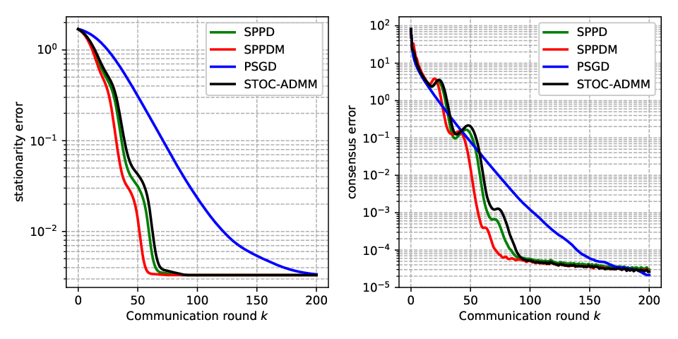
In Fig. 1, we observe that the SPPDM, SPPM and STOC-ADMM all perform better than the PSGD in terms of stationarity error and consensus error. The reason is that these methods all use constant step sizes rather than the diminishing step size. In addition, the proposed SPPDM has better performance than SPPD and STOC-ADMM, due to the Nesterov momentum.

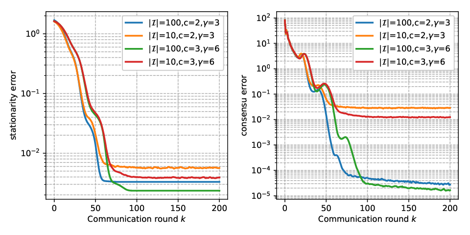
The impact of the mini-batch size $|\mathcal{I}|$ , and parameters $\gamma$ and $c$ are analyzed in Fig. 2. One can see that the larger mini-batch size we use, the smaller error we can achieve, which corroborates Corollary 1. With the same mini-batch size, the larger values of $\gamma$ and $c$ correspond to smaller primal and dual step sizes. Thus, the SPPDM with larger values of $\gamma$ and $c$ has slower convergence; whereas as seen from the figures, larger values of $\gamma$ and $c$ can lead to smaller stationarity error and consensus error.

For the offline setting, the comparison results of the proposed PPDM with the existing methods are shown in Fig. 3. It can be observed that the proposed PPDM enjoys the fastest convergence. Compared with the Prox-ADMM, it is clear to see the advantage of the PPDM with momentum for speeding up the algorithm convergence.

Refer to caption — Fig. 1: Comparison of proposed SPPDM with the PSGD and STOC-ADMM in terms of stationarity and consensus error; the batch size is $|\mathcal{I}|=100$ .

IV-B Distributed Neural Network

In this simulation, our task is to classify handwritten digits from the MNIST dataset. The local loss function $f_{i}(\theta_{i})$ in each node is the cross-entropy function. In this example, we do not consider nonsmooth term and inequality constraint set. Thus, many existing methods, D-PSGD [20], D² [21] and PR-SGD-M [27] can be applied to train a classification DNN.

Assume the neural network contains one hidden layer with 500 neurons. The $6\times 10^{4}$ training samples are divided into 10 subsets and assigned to the $N=10$ agents in two ways. The first is the IID case, where the samples are sufficiently shuffled, and then partitioned into 10 subsets with equal size ( $m=6000$ ). The second is the Non-IID case, where we first sort the samples according to their labels, divide it into 20 shards of size 3000, and assign each of 10 agents 2 shards. Thus most agents have samples of two digits only.

The communication graph is also a circle. We compare the SPPDM with the D-PSGD [20], D² [21] and PR-SGD-M [27]. The same mixing matrix in (52) is used for the three methods. Moreover, a fixed step size of $\ell=0.05$ is used to ensure the convergence of these three methods in the simulation. For the proposed SPPDM, we set parameter $c=1$ , $\gamma=3$ , $\alpha=0.001$ , $\kappa=0.1$ , $\beta=0.9$ , and $\eta_{k}=0.8$ . The batch size is $|\mathcal{I}|=128$ .

We calculate the loss value and the classification accuracy based on the average model $\bar{\theta}=1/N\sum_{i=1}^{N}\theta_{i}$ . Fig. 4 and Fig. 5 show the training loss and the classification accuracy for the IID case and Non-IID case by averaging over all 5 trials, respectively. From Fig. 4, we see that D² and D-PSGD have a similar performance; meanwhile, the proposed SPPD performs better than these two methods. Besides, one can see that SPPDM and PR-SGD-M enjoy fast decreasing of the loss function and increasing of the classification accuracy, respectively. The reason is that both SPPDM and PR-SGD-M use the momentum technique. We should point out that the communication overhead of PR-SGD-M is twice of the SPPDM since the PR-SGD-M requires the agents to exchange not only the variable $x_{i}$ but also the momentum variables. Lastly, comparing the SPPDM with SPPD, it shows again that the momentum techniques can accelerate the algorithm convergence.

From Fig. 5 for the non-IID case, we can observe that the D² performs better than D-PSGD and SPPD. In fact, by comparing the curves in Fig. 4 with those in Fig. 5, one can see that the convergence curve of D² remains almost the same due to the use of the variance reduction technique whereas D-PSGD and SPPD deteriorate under the non-IID setting. As seen, the convergence of SPPDM is also slowed, but it still performs best among the methods under test.

V Conclusion

In this paper, we have proposed a distributed stochastic proximal primal-dual algorithm with momentum for minimizing a non-convex and non-smooth function (5) over a connected multi-agent network. We have shown (in Remark 1 and Remark 2) that the proposed algorithm has a close connection with some of the existing algorithms that are for convex and smooth problems, and therefore can be regarded as an enhanced counterpart of these existing algorithms. Theoretically, under Assumptions 1-3, we have built the convergence conditions of the proposed algorithms in Theorem 1 and Theorem 2. In particular, we have shown that the proposed SPPDM can achieve an $\epsilon$ -stationary solution with $\mathcal{O}(1/\epsilon^{2})$ computational complexity and $\mathcal{O}(1/\epsilon)$ communication complexity, where the latter is better than many of the existing methods which have $\mathcal{O}(1/\epsilon^{2})$ communication complexity (see Table 1). Experimental results have demonstrated that the proposed algorithms with momentum can effectively speed up the convergence. For distributed learning under non-IID data distribution (Fig. 5), we have also shown the proposed SPPDM performs better than the existing methods.

As future research directions, one may further relax Assumption 3 to accommodate a larger class of regularization functions. Besides, it will be also interesting to investigate the trade-off between the communication complexity (as measured by the number of bits exchanged) and the convergence. Moreover, we will analytically investigate how data distribution affect the algorithm convergence and improve the robustness of the algorithms against to unbalanced and non-IID data distribution in the future.

Appendix A Derivation of (20)

When we remove the non-smooth regularization term $r({\bf x})$ , the proximal gradient update can be removed. Assume $\beta=1$ , then (31) can be written as

	$\displaystyle{\bf x}^{k+1}$	$\displaystyle={\bf\Psi}^{-1}\big(\gamma{\bf s}^{k}+c{\bf B}^{\top}{\bf B}{\bf x}^{k}+\kappa{\bf x}^{k}-\nabla f({\bf s}^{k})-{\bf A}^{\top}{\boldsymbol{\lambda}}^{k+1}\big)$
		$\displaystyle={\bf\Psi}^{-1}\big(\tilde{{\bf W}}{\bf s}^{k}-{\bf\Psi}^{-1}\nabla f({\bf s}^{k})+{\bf C}^{k}\big),$

where

	$\displaystyle\tilde{}{\bf W}$	$\displaystyle=c{\bf\Psi}^{-1}{\bf B}^{\top}{\bf B}+(\gamma+\kappa){\bf\Psi}^{-1},$		(53)
	$\displaystyle{\bf C}^{k}$	$\displaystyle={\bf\Psi}^{-1}(c{\bf B}^{\top}{\bf B}({\bf x}^{k}-{\bf s}^{k})+\kappa({\bf x}^{k}-{\bf s}^{k}))-{\bf\Psi}^{-1}{\bf A}^{\top}{\boldsymbol{\lambda}}^{k+1}.$		(54)

Using the definition of $\tilde{}{\bf U}=c{\bf\Psi}^{-1}{\bf B}^{\top}{\bf B}$ in (II-B), we rewrite (53) as

\displaystyle\tilde{}{\bf W}

\displaystyle=\tilde{}{\bf U}+{\bf\Psi}^{-1}(\gamma+\kappa){\bf I}.

According the definition of ${\bf\Psi}=(\gamma+\kappa){\bf I}+c({\bf A}^{\top}{\bf A}+{\bf B}^{T}{\bf B})$ and $c=\alpha$ , we have

\displaystyle{\bf I}-\tilde{}{\bf W}={\bf\Psi}^{-1}{\bf\Psi}-\tilde{}{\bf W}=\alpha{\bf\Psi}^{-1}{\bf A}^{\top}{\bf A}.

(55)

Based on

\displaystyle{\bf A}^{\top}{\boldsymbol{\lambda}}^{k+1}={\bf p}^{k+1}={\bf p}^{k}+\alpha{\bf A}^{\top}{\bf A}{\bf x}^{k},

(56)

if ${\bf p}^{0}=0$ , and applying (55), we obtain

\displaystyle{\bf\Psi}^{-1}{\bf A}^{\top}{\boldsymbol{\lambda}}^{k+1}=\sum_{t=0}^{k}\alpha{\bf\Psi}^{-1}{\bf A}^{\top}{\bf A}{\bf x}^{t}=\sum_{t=0}^{k}({\bf I}-\tilde{}{\bf W}){\bf x}^{t}.

By substituting the above equality into (54), we obtain (20).

Appendix B Proof of Theorem 1

Let us recapitulate the augmented Lagrange function in (24) below

	$\displaystyle L_{c}({\bf x},{\bf z};{\boldsymbol{\lambda}})=$	$\displaystyle f({\bf x})+r({\bf x})+\langle{\boldsymbol{\lambda}},{\bf A}{\bf x}\rangle$
		$\displaystyle+\frac{c}{2}\\|{\bf A}{\bf x}\\|^{2}+\frac{\kappa}{2}\\|{\bf x}-{\bf z}\\|^{2}.$		(57)

We introduce some auxiliary functions as follows

		$\displaystyle d({\bf z};{\boldsymbol{\lambda}})=\min_{{\bf x}}L_{c}({\bf x},{\bf z};{\boldsymbol{\lambda}})$		(58)
		$\displaystyle{\bf x}({\bf z};{\boldsymbol{\lambda}})=\mathop{\arg\min}_{{\bf x}}L_{c}({\bf x},{\bf z};{\boldsymbol{\lambda}})$		(59)
		$\displaystyle P({\bf z})=\min_{\begin{subarray}{c}{\bf A}{\bf x}=0\end{subarray}}f({\bf x})+r({\bf x})+\frac{\kappa}{2}\\|{\bf x}-{\bf z}\\|^{2}$		(60)
		$\displaystyle{\bf x}({\bf z})=\mathop{\arg\min}_{\begin{subarray}{c}{\bf A}{\bf x}=0\end{subarray}}f({\bf x})+r({\bf x})+\frac{\kappa}{2}\\|{\bf x}-{\bf z}\\|^{2}.$		(61)

Besides, we define the full gradient iterate $\hat{{\bf x}}^{k+1}$ and $\hat{{\bf z}}^{k+1}$ ,

	$\displaystyle\hat{{\bf x}}^{k+1}$	$\displaystyle:=\mathop{\arg\min}_{{\bf x}}g({\bf x},{\bf w}^{k};{\boldsymbol{\lambda}}^{k+1})$		(62)
	$\displaystyle\hat{{\bf z}}^{k+1}$	$\displaystyle:={\bf z}^{k}+\beta(\hat{{\bf x}}^{k+1}-{\bf z}^{k}),$		(63)

where ${\bf w}^{k}=[{\bf x}^{k},{\bf s}^{k},{\bf z}^{k}]$ and

		$\displaystyle g({\bf x},{\bf w}^{k};{\boldsymbol{\lambda}}^{k+1})$
		$\displaystyle=f({\bf s}^{k})+\langle\nabla f({\bf s}^{k}),{\bf x}-{\bf s}^{k}\rangle+\frac{\gamma}{2}\\|{\bf x}-{\bf s}^{k}\\|^{2}+r({\bf x})$
		$\displaystyle+\langle{\boldsymbol{\lambda}}^{k+1},{\bf A}{\bf x}\rangle+\frac{c}{2}\\|{\bf A}{\bf x}\\|^{2}+\frac{c}{2}\\|{\bf x}-{\bf x}^{k}\\|_{{\bf B}^{\top}{\bf B}}^{2}+\frac{\kappa}{2}\\|{\bf x}-{\bf z}^{k}\\|^{2}.$		(64)

We also define

\displaystyle g({\bf x},{\bf w}^{k},{\boldsymbol{\xi}}^{k};{\boldsymbol{\lambda}}^{k+1})

\displaystyle:=g({\bf x},{\bf x}^{k},{\bf s}^{k},{\bf z}^{k},{\boldsymbol{\xi}}^{k};{\boldsymbol{\lambda}}^{k+1})

for (30) at our disposal.

B-A Some Error Bounds

Firstly, we show the upper bound between ${\bf x}^{k+1}$ and $\hat{{\bf x}}^{k+1}$ .

Lemma 1.

Suppose Assumption 3 holds, we have

\displaystyle\mathbb{E}[\|{\bf x}^{k+1}-\hat{{\bf x}}^{k+1}\|^{2}]\leq\frac{{N\sigma^{2}}}{(\gamma+2c+\kappa)^{2}|\mathcal{I}|}.

(65)

Proof.

According to (42)-(43) in Assumption 3, we know

\displaystyle\mathbb{E}\Big[\big\|\frac{1}{|\mathcal{I}|}\sum_{j=1}^{|\mathcal{I}|}G({\bf s}^{k},{\boldsymbol{\xi}}_{j}^{k})-\nabla f({\bf x})\big\|^{2}\Big]\leq\frac{N}{|\mathcal{I}|}\sigma^{2}.

(66)

In addition, like (31), the proximity form of (62) is

	$\displaystyle\hat{{\bf x}}^{k+1}$	$\displaystyle=\textmd{prox}_{r}^{{\bf\Psi}}\Big({\bf\Psi}^{-1}\big(\gamma{\bf s}^{k}+c{\bf B}^{\top}{\bf B}{\bf x}^{k}+\kappa{\bf z}^{k}$
		$\displaystyle\qquad\qquad-\nabla f({\bf s}^{k})-{\bf A}^{\top}{\boldsymbol{\lambda}}^{k+1}\big)\Big).$		(67)

Using (31), (66)-(67) and applying the nonexpansive property of the proximal operator (see for example [30, p. 340]) we then obtain (65). ∎

Lemma 2.

Suppose $\kappa>-\mu$ . There exists some positive constants $\sigma_{1}$ , $\sigma_{2}$ such that the following primal error bound holds

\displaystyle\!\!\!\!\|{\bf x}^{k}-{\bf x}({\bf z}^{k};{\boldsymbol{\lambda}}^{k+1})\|\leq\sigma_{1}\|{\bf x}^{k}-\hat{{\bf x}}^{k+1}\|+\sigma_{2}\|{\bf x}^{k}-{\bf s}^{k}\|.

(68)

Proof.

Based on $\kappa>-\mu$ , we know that $L_{c}$ in (57) is strongly convex in ${\bf x}$ with modulus $\kappa+\mu$ and Lipschitz constant $\kappa+L+c\sigma_{A}^{2}$ , where $\sigma_{A}$ is the spectral norm of the matrix. Thus, we can apply [31, Theorem 3.1] to upper bound the distance between ${\bf x}^{k}$ and the optimal solution ${\bf x}({\bf z}^{k};{\boldsymbol{\lambda}}^{k+1})$

\displaystyle\|{\bf x}^{k}-{\bf x}({\bf z}^{k};{\boldsymbol{\lambda}}^{k+1})\|\leq\varrho\|\tilde{\nabla}_{{\bf x}}L_{c}({\bf x}^{k},{\bf z}^{k};{\boldsymbol{\lambda}}^{k+1})\|,

(69)

where $\varrho=\frac{\kappa+L+c\sigma_{A}^{2}+1}{\kappa+\mu}$ and

\displaystyle\tilde{\nabla}_{{\bf x}}L_{c}({\bf x},{\bf z};{\boldsymbol{\lambda}})={\bf x}-\textmd{prox}_{r}^{{\bf\Psi}}({\bf x}-\nabla_{{\bf x}}(L_{c}({\bf x},{\bf z};{\boldsymbol{\lambda}})-r({\bf x})))

is known as the proximal gradient.

We can bound $\|\tilde{\nabla}_{{\bf x}}L_{c}({\bf x}^{k},{\bf z}^{k};{\boldsymbol{\lambda}}^{k+1})\|$ as follows

		$\displaystyle\\|\tilde{\nabla}_{{\bf x}}L_{c}({\bf x}^{k},{\bf z}^{k};{\boldsymbol{\lambda}}^{k+1})\\|$
		$\displaystyle=\\|{\bf x}^{k}-\textmd{prox}_{r}^{{\bf\Psi}}({\bf x}^{k}-\nabla_{{\bf x}}(L_{c}({\bf x}^{k},{\bf z}^{k};{\boldsymbol{\lambda}}^{k+1})-r({\bf x}^{k})))\\|$
		$\displaystyle\leq\\|{\bf x}^{k}-\hat{{\bf x}}^{k+1}\\|$
		$\displaystyle~~~+\\|\hat{{\bf x}}^{k+1}-\textmd{prox}_{r}^{{\bf\Psi}}({\bf x}^{k}-\nabla_{{\bf x}}(L_{c}({\bf x}^{k},{\bf z}^{k};{\boldsymbol{\lambda}}^{k+1})-r({\bf x}^{k})))\\|$
		$\displaystyle=\\|{\bf x}^{k}-\hat{{\bf x}}^{k+1}\\|$
		$\displaystyle~~~+\Big\\|\textmd{prox}_{r}^{{\bf\Psi}}(\hat{{\bf x}}^{k+1}-\nabla_{{\bf x}}(g(\hat{{\bf x}}^{k+1},{\bf w}^{k};{\boldsymbol{\lambda}}^{k+1})-r(\hat{{\bf x}}^{k+1})))$
		$\displaystyle~~~-\textmd{prox}_{r}^{{\bf\Psi}}({\bf x}^{k}-\nabla_{{\bf x}}(L_{c}({\bf x}^{k},{\bf z}^{k};{\boldsymbol{\lambda}}^{k+1})-r({\bf x}^{k})))\Big\\|$
		$\displaystyle\leq(2+2cd_{\max}+\gamma+\kappa)\\|{\bf x}^{k}-\hat{{\bf x}}^{k+1}\\|+(\gamma+L)\\|{\bf x}^{k}-{\bf s}^{k}\\|,$

where $d_{\max}=\max\{d_{1},\ldots,d_{N}\}$ ; the second equality is obtained by using the optimality condition of $\hat{{\bf x}}^{k+1}$ in (62), and the second inequality is based on the nonexpansive property of the proximal operator. Denote

	$\displaystyle\sigma_{1}$	$\displaystyle=\varrho(2+2cd_{\max}+\gamma+\kappa),$		(70)
	$\displaystyle\sigma_{2}$	$\displaystyle=\gamma+L.$		(71)

The proof is complete. ∎

Lemma 3.

(Lemma 3.2 in [17]) Suppose $\kappa>-\mu$ , and Assumption 1 holds. There exists some positive constants $\sigma_{3},\sigma_{4}$ such that the following error bounds hold

	$\displaystyle\\|{\boldsymbol{\lambda}}_{1}-{\boldsymbol{\lambda}}_{2}\\|$	$\displaystyle\geq\sigma_{3}\\|{\bf x}({\bf z};{\boldsymbol{\lambda}}_{1})-{\bf x}({\bf z};{\boldsymbol{\lambda}}_{2})\\|$		(72)
	$\displaystyle\\|{\bf z}_{1}-{\bf z}_{2}\\|$	$\displaystyle\geq\sigma_{4}\\|{\bf x}({\bf z}_{1};{\boldsymbol{\lambda}})-{\bf x}({\bf z}_{2};{\boldsymbol{\lambda}})\\|,$		(73)

where

	$\displaystyle\sigma_{3}$	$\displaystyle=(\kappa+\mu)/\sigma_{A}$		(74)
	$\displaystyle\sigma_{4}$	$\displaystyle=(\kappa+\mu)/\kappa.$		(75)

Lemma 4.

Suppose that Assumptions 1-2 hold and $\kappa>\mu$ . Then, there exist some positive scalars $\sigma_{5}$ , $\Delta$ such that the following dual error bound holds

\displaystyle\|{\bf x}({\bf z},{\boldsymbol{\lambda}})-{\bf x}({\bf z})\|\leq\sigma_{5}\|{\bf A}{\bf x}({\bf z};{\boldsymbol{\lambda}})\|,~for~any~{\bf z},~{\boldsymbol{\lambda}}.

(76)

where $\sigma_{5}$ depends only on the constants $L,\kappa,\sigma_{A},\mu$ and the matrices ${\bf A},{\bf S}_{x},{\bf S}_{y}$ .

Proof.

The lemma is an extension of [18, Lemma 3.2], where the non-smooth term $r({\bf x})$ of (5) is limited to an indicator function of a polyhedral set. Due to limited space, the proof details are relegated to the supplementary document [32]. ∎

B-B Decent Lemmas

In order to show the convergence of Algorithm 1, we consider a new potential function,

	$\displaystyle\mathbb{E}[\phi^{k+1}]$	$\displaystyle\triangleq\mathbb{E}[L_{c}({\bf x}^{k+1},{\bf z}^{k+1};{\boldsymbol{\lambda}}^{k+1})+\tau\\|{\bf x}^{k+1}-{\bf x}^{k}\\|^{2}]$
		$\displaystyle~~~+\mathbb{E}[2P({\bf z}^{k+1})-2d({\bf z}^{k+1};{\boldsymbol{\lambda}}^{k+1})],$		(77)

for some $\tau>0$ . By the weak duality, we have

\displaystyle L_{c}({\bf x},{\bf z};{\boldsymbol{\lambda}})\geq d({\bf z};{\boldsymbol{\lambda}}),P({\bf z})\geq d({\bf z};{\boldsymbol{\lambda}}).

(78)

Thus, we have $\mathbb{E}[\phi^{k}]\geq\mathbb{E}[P({\bf z}^{k})]$ . According to the definition of $P({\bf z}^{k})$ in (60) and Assumption 1 (ii), we obtain $P({\bf z}^{k})\geq\underline{f}$ . As a result, $\mathbb{E}[\phi^{k}]$ is bounded below by $\underline{f}$ .

Lemma 5.

For a sequence $\{{\bf x}^{k},{\bf z}^{k},{\boldsymbol{\lambda}}^{k}\}$ generated by Algorithm 1, if $\kappa>-\mu$ , $\gamma>3L$ , $0<\beta<1$ and

\displaystyle 0\leq\eta_{k}\leq\sqrt{\frac{\kappa+2c+\gamma-3L}{2(\gamma-\mu+3L)}}:=\bar{\eta},

(79)

there exit some positive constants $\tau$ , $\hat{\sigma}_{1}$ and $\hat{\sigma}_{2}$ such that

	$\displaystyle\hat{\sigma}_{1}$	$\displaystyle\triangleq\frac{\kappa+2c+\gamma-3L}{2}-2\tau\geq 0$		(80)
	$\displaystyle\hat{\sigma}_{2}$	$\displaystyle\triangleq\frac{\mu-\gamma-3L}{2}{\bar{\eta}}^{2}+\tau\geq 0,$		(81)

then

		$\displaystyle\mathbb{E}[L_{c}({\bf x}^{k},{\bf z}^{k};{\boldsymbol{\lambda}}^{k})+\tau\\|{\bf x}^{k}-{\bf x}^{k-1}\\|^{2}]$
		$\displaystyle~~~-\mathbb{E}[L_{c}({\bf x}^{k+1},{\bf z}^{k+1};{\boldsymbol{\lambda}}^{k+1})-\tau\\|{\bf x}^{k+1}-{\bf x}^{k}\\|^{2}]$
		$\displaystyle\geq-\alpha\mathbb{E}[\\|{\bf A}{\bf x}^{k}\\|^{2}]+\frac{\kappa}{2\beta}\mathbb{E}[\\|{\bf z}^{k}-{\bf z}^{k+1}\\|^{2}]$
		$\displaystyle~~~+\hat{\sigma}_{1}\mathbb{E}[\\|{\bf x}^{k}-\hat{{\bf x}}^{k+1}\\|^{2}]+\hat{\sigma}_{2}\mathbb{E}[\\|{\bf x}^{k}-{\bf x}^{k-1}\\|^{2}]$
		$\displaystyle~~~-\left(\frac{1}{2\gamma}+\frac{3L+4\tau}{2(\gamma+2c+\kappa)^{2}}\right)\frac{N\sigma^{2}}{\|\mathcal{I}\|}.$		(82)

Proof.

Firstly, according to (24) and (26), we have

\displaystyle\!\!\!\!\mathbb{E}[L_{c}({\bf x}^{k},{\bf z}^{k};{\boldsymbol{\lambda}}^{k})-L_{c}({\bf x}^{k},{\bf z}^{k};{\boldsymbol{\lambda}}^{k+1})]=-\alpha\mathbb{E}[\|{\bf A}{\bf x}^{k}\|^{2}].

(83)

Secondly, we have

		$\displaystyle\mathbb{E}[L_{c}({\bf x}^{k},{\bf z}^{k};{\boldsymbol{\lambda}}^{k+1})-L_{c}({\bf x}^{k+1},{\bf z}^{k};{\boldsymbol{\lambda}}^{k+1})]$
		$\displaystyle=\mathbb{E}[L_{c}({\bf x}^{k},{\bf z}^{k};{\boldsymbol{\lambda}}^{k+1})-g({\bf x}^{k},{\bf w}^{k};{\boldsymbol{\lambda}}^{k+1})]$
		$\displaystyle~~~+\mathbb{E}[g({\bf x}^{k},{\bf w}^{k}{\boldsymbol{\lambda}}^{k+1})-g(\hat{{\bf x}}^{k+1},{\bf w}^{k};{\boldsymbol{\lambda}}^{k+1})]$
		$\displaystyle~~~+\mathbb{E}[g(\hat{{\bf x}}^{k+1},{\bf w}^{k};{\boldsymbol{\lambda}}^{k+1})-g({\bf x}^{k+1},{\bf w}^{k},{\boldsymbol{\xi}}^{k};{\boldsymbol{\lambda}}^{k+1})]$
		$\displaystyle~~~+\mathbb{E}[g({\bf x}^{k+1},{\bf w}^{k},{\boldsymbol{\xi}}^{k};{\boldsymbol{\lambda}}^{k+1})-L_{c}({\bf x}^{k+1},{\bf z}^{k};{\boldsymbol{\lambda}}^{k+1})].$		(84)

Next, we bound each of the terms in the right hand side of (84). Based on the definition of function $g$ in (64), we have

		$\displaystyle\mathbb{E}[L_{c}({\bf x}^{k},{\bf z}^{k};{\boldsymbol{\lambda}}^{k+1})-g({\bf x}^{k},{\bf w}^{k};{\boldsymbol{\lambda}}^{k+1})]$
		$\displaystyle=\mathbb{E}[f({\bf x}^{k})-f({\bf s}^{k})-\langle\nabla f({\bf s}^{k}),{\bf x}^{k}-{\bf s}^{k}\rangle-\frac{\gamma}{2}\\|{\bf x}^{k}-{\bf s}^{k}\\|^{2}]$
		$\displaystyle\geq\frac{\mu-\gamma}{2}\mathbb{E}[\\|{\bf x}^{k}-{\bf s}^{k}\\|^{2}],$		(85)

where the inequality comes from (38) in Assumption 1. Using the strongly convexity of the objective function $g$ (with modulus $\kappa+2c+\gamma$ ) and the definition of $\hat{{\bf x}}^{k+1}$ in (62), we can obtain

		$\displaystyle\mathbb{E}[g({\bf x}^{k},{\bf w}^{k};{\boldsymbol{\lambda}}^{k+1})-g(\hat{{\bf x}}^{k+1},{\bf w}^{k};{\boldsymbol{\lambda}}^{k+1})]$
		$\displaystyle\geq\frac{\kappa+2c+\gamma}{2}\mathbb{E}[\\|{\bf x}^{k}-\hat{{\bf x}}^{k+1}\\|^{2}].$		(86)

In addition, we have

		$\displaystyle\mathbb{E}[g(\hat{{\bf x}}^{k+1},{\bf w}^{k};{\boldsymbol{\lambda}}^{k+1})-g({\bf x}^{k+1},{\bf w}^{k},{\boldsymbol{\xi}}^{k};{\boldsymbol{\lambda}}^{k+1})]$
		$\displaystyle=\mathbb{E}[g(\hat{{\bf x}}^{k+1},{\bf w}^{k},{\boldsymbol{\xi}}^{k};{\boldsymbol{\lambda}}^{k+1})-g({\bf x}^{k+1},{\bf w}^{k},{\boldsymbol{\xi}}^{k};{\boldsymbol{\lambda}}^{k+1})]$
		$\displaystyle\geq 0,$		(87)

where the first equality dues to (42) in Assumption 3, and the above inequality dues to ${\bf x}^{k+1}$ is the optimal solution in (28). Lastly, we can bound

		$\displaystyle\mathbb{E}[g({\bf x}^{k+1},{\bf w}^{k},{\boldsymbol{\xi}}^{k};{\boldsymbol{\lambda}}^{k+1})-L_{c}({\bf x}^{k+1},{\bf z}^{k};{\boldsymbol{\lambda}}^{k+1})]$
		$\displaystyle=\mathbb{E}[f({\bf s}^{k})]+\frac{1}{\|\mathcal{I}\|}\sum_{j=1}^{\|\mathcal{I}\|}\mathbb{E}[\langle G({\bf s}^{k},{\boldsymbol{\xi}}_{j}^{k}),{\bf x}^{k+1}-{\bf s}^{k}\rangle]$
		$\displaystyle~~~+\mathbb{E}\left[\frac{\gamma}{2}\\|{\bf x}^{k+1}-{\bf s}^{k}\\|^{2}]+\frac{c}{2}\\|{\bf x}^{k+1}-{\bf x}^{k}\\|_{{\bf B}^{\top}{\bf B}}^{2}-f({\bf x}^{k+1})\right]$
		$\displaystyle\geq\frac{1}{\|\mathcal{I}\|}\sum_{j=1}^{\|\mathcal{I}\|}\mathbb{E}[\langle G({\bf s}^{k},{\boldsymbol{\xi}}_{j}^{k})-\nabla f({\bf s}^{k}),{\bf x}^{k+1}-{\bf s}^{k}\rangle]$
		$\displaystyle~~~+\frac{\gamma-L}{2}\mathbb{E}[\\|{\bf x}^{k+1}-{\bf s}^{k}\\|^{2}]+\frac{c}{2}\mathbb{E}[\\|{\bf x}^{k+1}-{\bf x}^{k}\\|_{{\bf B}^{\top}{\bf B}}^{2}]$
		$\displaystyle\geq-\frac{N\sigma^{2}}{2\gamma\|\mathcal{I}\|}-\frac{L}{2}\mathbb{E}[\\|{\bf x}^{k+1}-{\bf s}^{k}\\|^{2}],$		(88)

where the first inequality is obtained by applying the descent lemma [33, Lemma1.2.3]

\displaystyle f({\bf x}^{k+1})\leq f({\bf s}^{k})+\langle\nabla f({\bf s}^{k}),{\bf x}^{k+1}-{\bf s}^{k}\rangle+\frac{L}{2}\|{\bf x}^{k+1}-{\bf s}^{k}\|^{2}

owing to gradient Lipschitz continuity in (37); the second inequality holds by using the Young’s inequality $a^{\top}b\geq-\frac{\|a\|^{2}}{2\gamma}-\frac{\gamma\|b\|^{2}}{2}$ and (43) in Assumption 3. Using the convexity of the operator $\|\cdot\|^{2}$ , we have

	$\displaystyle\\|{\bf x}^{k+1}-{\bf s}^{k}\\|^{2}\leq$	$\displaystyle 3\\|{\bf x}^{k+1}-\hat{{\bf x}}^{k+1}\\|^{2}+3\\|\hat{{\bf x}}^{k+1}-{\bf x}^{k}\\|^{2}$
		$\displaystyle+3\\|{\bf x}^{k}-{\bf s}^{k}\\|^{2}.$		(89)

Substituting (65) and (89) into (88) gives rise to

		$\displaystyle\mathbb{E}[g({\bf x}^{k+1},{\bf w}^{k},{\boldsymbol{\xi}}^{k};{\boldsymbol{\lambda}}^{k+1})-L_{c}({\bf x}^{k+1},{\bf z}^{k};{\boldsymbol{\lambda}}^{k+1})]$
		$\displaystyle\geq-\left(\frac{1}{2\gamma}+\frac{3L}{2(\gamma+2c+\kappa)^{2}}\right)\frac{N\sigma^{2}}{\|\mathcal{I}\|}$
		$\displaystyle~~~-\frac{3L}{2}\mathbb{E}[\\|\hat{{\bf x}}^{k+1}-{\bf x}^{k}\\|^{2}]-\frac{3L}{2}\mathbb{E}[\\|{\bf s}^{k}-{\bf x}^{k}\\|^{2}].$		(90)

By further substituting (85)-(87) and (90) into (84), we obtain

		$\displaystyle\mathbb{E}[L_{c}({\bf x}^{k},{\bf z}^{k};{\boldsymbol{\lambda}}^{k+1})+\tau\\|{\bf x}^{k}-{\bf x}^{k-1}\\|^{2}$
		$\displaystyle~~~-L_{c}({\bf x}^{k+1},{\bf z}^{k};{\boldsymbol{\lambda}}^{k+1})-\tau\\|{\bf x}^{k+1}-{\bf x}^{k}\\|^{2}]$
		$\displaystyle\geq\frac{\mu-\gamma}{2}\mathbb{E}[\\|{\bf x}^{k}-{\bf s}^{k}\\|^{2}]+\frac{\kappa+2c+\gamma}{2}\mathbb{E}[\\|{\bf x}^{k}-\hat{{\bf x}}^{k+1}\\|^{2}]$
		$\displaystyle~~~-\frac{3L}{2}\mathbb{E}[\\|\hat{{\bf x}}^{k+1}-{\bf x}^{k}\\|^{2}]-\frac{3L}{2}\mathbb{E}[\\|{\bf s}^{k}-{\bf x}^{k}\\|^{2}]$
		$\displaystyle~~~-\left(\frac{1}{2\gamma}+\frac{3L}{2(\gamma+2c+\kappa)^{2}}\right)\frac{\sigma^{2}}{\|\mathcal{I}\|}+\tau\mathbb{E}[\\|{\bf x}^{k}-{\bf x}^{k-1}\\|^{2}]$
		$\displaystyle~~~-2\tau\mathbb{E}[\\|{\bf x}^{k+1}-\hat{{\bf x}}^{k+1}\\|^{2}]-2\tau\mathbb{E}[\\|\hat{{\bf x}}^{k+1}-{\bf x}^{k}\\|^{2}]$
		$\displaystyle=\hat{\sigma}_{1}\mathbb{E}[\\|{\bf x}^{k}-\hat{{\bf x}}^{k+1}\\|^{2}]+\hat{\sigma}_{2}\mathbb{E}[\\|{\bf x}^{k}-{\bf x}^{k-1}\\|^{2}]$
		$\displaystyle~~~-\left(\frac{1}{2\gamma}+\frac{3L+4\tau}{2(\gamma+2c+\kappa)^{2}}\right)\frac{N\sigma^{2}}{\|\mathcal{I}\|},$		(91)

where $\hat{\sigma}_{1}$ and $\hat{\sigma}_{2}$ are defined in (80) and (81), respectively, and the equality is obtained by applying (27).

Thirdly, according to the definition of the ${\bf z}$ update in (29), we have

		$\displaystyle\mathbb{E}[L_{c}({\bf x}^{k+1},{\bf z}^{k};{\boldsymbol{\lambda}}^{k+1})-L_{c}({\bf x}^{k+1},{\bf z}^{k+1};{\boldsymbol{\lambda}}^{k+1})]$
		$\displaystyle\geq\frac{\kappa}{2\beta}(2-\beta)\mathbb{E}[\\|{\bf z}^{k}-{\bf z}^{k+1}\\|^{2}]$
		$\displaystyle\geq\frac{\kappa}{2\beta}\mathbb{E}[\\|{\bf z}^{k}-{\bf z}^{k+1}\\|^{2}],$		(92)

where the last inequality is due to $0<\beta<1$ . By combining (83), (91) and (B-B), we obtain (82). Besides, (80) and (81) implies (79). ∎

Lemma 6.

Under Assumptions 1-3, if $\kappa>-\mu$ , $\gamma>3L$ , $\eta_{k}$ is a constant satisfies the condition (47), and

	$\displaystyle 0<\alpha\leq\min\left\{\frac{\hat{\sigma}_{1}}{4\sigma_{A}\sigma_{1}^{2}},\frac{\hat{\sigma}_{2}}{4\sigma_{A}^{2}\sigma_{2}^{2}\eta_{k}^{2}},c\right\},$		(93)
	$\displaystyle 0<\beta<\min\left\{\frac{\alpha}{12\kappa\sigma_{5}^{2}},\frac{\sigma_{4}}{36},1\right\},$		(94)

where $\sigma_{1}$ , $\sigma_{2}$ , $\sigma_{4}$ and $\sigma_{5}$ are constants denoted in (70) and (71), (75) and (76), respectively. Then we have

		$\displaystyle\mathbb{E}[\phi^{k}-\phi^{k+1}]$
		$\displaystyle\geq\frac{\kappa(1-\beta)\beta}{4}\mathbb{E}[\\|\hat{{\bf x}}^{k+1}-{\bf z}^{k}\\|^{2}]+\frac{\alpha}{2}\mathbb{E}[\\|{\bf A}{\bf x}({\bf z}^{k},{\boldsymbol{\lambda}}^{k+1})\\|^{2}]$
		$\displaystyle+\frac{\hat{\sigma}_{1}}{2}\mathbb{E}[\\|{\bf x}^{k}-\hat{{\bf x}}^{k+1}\\|^{2}]+\frac{\hat{\sigma}_{2}}{2}\mathbb{E}[\\|{\bf x}^{k}-{\bf x}^{k-1}\\|^{2}]-\frac{C_{1}N\sigma^{2}}{\|\mathcal{I}\|},$		(95)

where $\hat{{\bf x}}^{k+1}$ and $\hat{{\bf z}}^{k+1}$ are defined in (62) and (63), and

\displaystyle C_{1}=\left(\frac{1}{2\gamma}+\frac{6L+8\tau+\kappa(1-\beta)}{4(\gamma+2c+\kappa)^{2}}\right).

(96)

Proof.

From the definition of $d({\bf z};{\boldsymbol{\lambda}})$ in (58), we have

		$\displaystyle\mathbb{E}[d({\bf z}^{k};{\boldsymbol{\lambda}}^{k+1})-d({\bf z}^{k};{\boldsymbol{\lambda}}^{k})]$
		$\displaystyle=\mathbb{E}[L_{c}({\bf x}({\bf z}^{k};{\boldsymbol{\lambda}}^{k+1}),{\bf z}^{k};{\boldsymbol{\lambda}}^{k+1})-L_{c}({\bf x}({\bf z}^{k};{\boldsymbol{\lambda}}^{k}),{\bf z}^{k};{\boldsymbol{\lambda}}^{k})]$
		$\displaystyle\geq\mathbb{E}[L_{c}({\bf x}({\bf z}^{k};{\boldsymbol{\lambda}}^{k+1}),{\bf z}^{k};{\boldsymbol{\lambda}}^{k+1})-L_{c}({\bf x}({\bf z}^{k};{\boldsymbol{\lambda}}^{k+1}),{\bf z}^{k};{\boldsymbol{\lambda}}^{k})]$
		$\displaystyle=\alpha\mathbb{E}[\langle{\bf A}{\bf x}^{k},{\bf A}{\bf x}({\bf z}^{k},{\boldsymbol{\lambda}}^{k+1})\rangle],$

where the inequality is due to ${\bf x}({\bf z}^{k};{\boldsymbol{\lambda}}^{k})=\arg\min_{{\bf x}}L_{c}({\bf x},{\bf z}^{k};{\boldsymbol{\lambda}}^{k})$ and the second equality comes from the iterates in (26). Using a similar technique, we have

		$\displaystyle\mathbb{E}[d({\bf z}^{k+1};{\boldsymbol{\lambda}}^{k+1})-d({\bf z}^{k};{\boldsymbol{\lambda}}^{k+1})]$
		$\displaystyle\geq\frac{\kappa}{2}\mathbb{E}[({\bf z}^{k+1}-{\bf z}^{k})^{\top}({\bf z}^{k+1}+{\bf z}^{k}-2{\bf x}({\bf z}^{k+1},{\boldsymbol{\lambda}}^{k+1}))].$

Combing the above two inequalities, we know

		$\displaystyle\mathbb{E}[d({\bf z}^{k+1};{\boldsymbol{\lambda}}^{k+1})-d({\bf z}^{k};{\boldsymbol{\lambda}}^{k})]$
		$\displaystyle\geq\alpha\mathbb{E}[\langle{\bf A}{\bf x}^{k},{\bf A}{\bf x}({\bf z}^{k},{\boldsymbol{\lambda}}^{k+1})\rangle]$		(97)
		$\displaystyle~~~+\frac{\kappa}{2}\mathbb{E}[({\bf z}^{k+1}-{\bf z}^{k})^{\top}({\bf z}^{k+1}+{\bf z}^{k}-2{\bf x}({\bf z}^{k+1},{\boldsymbol{\lambda}}^{k+1}))].$

Based on Danskin’s theorem [34, Proposition B.25] in convex analysis and $P({\bf z})$ defined in (60) with $\kappa>-\mu$ , we can have

\nabla P({\bf z}^{k})=\kappa({\bf z}^{k}-{\bf x}({\bf z}^{k})).

Thus, it shows

		$\displaystyle\\|\nabla P({\bf z}^{k})-\nabla P({\bf z}^{k+1})\\|$
		$\displaystyle\leq\kappa\\|{\bf z}^{k}-{\bf z}^{k+1}\\|+\kappa\\|{\bf x}({\bf z}^{k+1})-{\bf x}({\bf z}^{k})\\|$
		$\displaystyle\leq\kappa\tilde{\sigma}_{4}\\|{\bf z}^{k+1}-{\bf z}^{k}\\|,$

where $\tilde{\sigma}_{4}=1+\sigma_{4}^{-1}$ and the final inequality is due to Lemma 3. The above inequality shows the gradient of $P({\bf z}^{k})$ is Lipschitz continuous, which therefore it satisfies the descent lemma

		$\displaystyle\mathbb{E}[P({\bf z}^{k+1})-P({\bf z}^{k})]$		(98)
		$\displaystyle\leq\mathbb{E}[\kappa({\bf z}^{k+1}-{\bf z}^{k})^{\top}({\bf z}^{k}-{\bf x}({\bf z}^{k}))]+\frac{\kappa\tilde{\sigma}_{4}}{2}\mathbb{E}[\\|{\bf z}^{k+1}-{\bf z}^{k}\\|^{2}].$

By combining (97), (98) and (82), we obtain

		$\displaystyle\mathbb{E}[\phi^{k}-\phi^{k+1}]$
		$\displaystyle\geq-\alpha\mathbb{E}[\\|{\bf A}{\bf x}^{k}\\|^{2}]+\frac{\kappa}{2\beta}\mathbb{E}[\\|{\bf z}^{k}-{\bf z}^{k+1}\\|^{2}]$
		$\displaystyle~~~+\hat{\sigma}_{1}\mathbb{E}[\\|{\bf x}^{k}-\hat{{\bf x}}^{k+1}\\|^{2}]-2\mathbb{E}[\kappa({\bf z}^{k+1}-{\bf z}^{k})^{\top}({\bf z}^{k}-{\bf x}({\bf z}^{k}))]$
		$\displaystyle~~~+\hat{\sigma}_{2}\mathbb{E}[\\|{\bf x}^{k}-{\bf x}^{k-1}\\|^{2}]-\left(\frac{1}{2\gamma}+\frac{3L+4\tau}{2(\gamma+2c+\kappa)^{2}}\right)\frac{N\sigma^{2}}{\|\mathcal{I}\|}$
		$\displaystyle~~~-\kappa\tilde{\sigma}_{4}\mathbb{E}[\\|{\bf z}^{k+1}-{\bf z}^{k}\\|^{2}]+2\alpha\mathbb{E}[\langle{\bf A}{\bf x}^{k},{\bf A}{\bf x}({\bf z}^{k},{\boldsymbol{\lambda}}^{k+1})\rangle]$
		$\displaystyle~~~+\kappa\mathbb{E}[({\bf z}^{k+1}-{\bf z}^{k})^{\top}({\bf z}^{k+1}+{\bf z}^{k}-2{\bf x}({\bf z}^{k+1},{\boldsymbol{\lambda}}^{k+1}))]$
		$\displaystyle=\alpha\mathbb{E}[\\|{\bf A}{\bf x}({\bf z}^{k},{\boldsymbol{\lambda}}^{k+1})\\|^{2}]-\alpha\mathbb{E}[\\|{\bf A}({\bf x}^{k}-{\bf x}({\bf z}^{k},{\boldsymbol{\lambda}}^{k+1}))\\|^{2}]$
		$\displaystyle~~~+\hat{\sigma}_{1}\mathbb{E}[\\|{\bf x}^{k}-\hat{{\bf x}}^{k+1}\\|^{2}]+(\frac{\kappa}{2\beta}+\kappa-\kappa\tilde{\sigma}_{4})\mathbb{E}[\\|{\bf z}^{k+1}-{\bf z}^{k}\\|^{2}]$
		$\displaystyle~~~+2\kappa\mathbb{E}[({\bf z}^{k+1}-{\bf z}^{k})^{\top}({\bf x}({\bf z}^{k})-{\bf x}({\bf z}^{k+1};{\boldsymbol{\lambda}}^{k+1}))]$
		$\displaystyle~~~+\hat{\sigma}_{2}\mathbb{E}[\\|{\bf x}^{k}-{\bf x}^{k-1}\\|^{2}]-\left(\frac{1}{2\gamma}+\frac{3L+4\tau}{2(\gamma+2c+\kappa)^{2}}\right)\frac{N\sigma^{2}}{\|\mathcal{I}\|},$		(99)

where the equality comes from completing the square

		$\displaystyle\mathbb{E}[\\|{\bf A}({\bf x}^{k}-{\bf x}({\bf z}^{k},{\boldsymbol{\lambda}}^{k+1}))\\|^{2}]$
		$\displaystyle=\mathbb{E}[\\|{\bf A}{\bf x}^{k}\\|^{2}-2\langle{\bf A}{\bf x}^{k},{\bf A}vx({\bf z}^{k},{\boldsymbol{\lambda}}^{k+1})+\\|{\bf A}{\bf x}({\bf z}^{k},{\boldsymbol{\lambda}}^{k+1})\\|^{2}\rangle].$

We further bound the right-hand-side terms of (99). By using the Young’s inequality, we have

		$\displaystyle 2({\bf z}^{k+1}-{\bf z}^{k})^{\top}({\bf x}({\bf z}^{k})-{\bf x}({\bf z}^{k};{\boldsymbol{\lambda}}^{k+1}))$
		$\displaystyle\geq-\frac{\\|{\bf z}^{k+1}-{\bf z}^{k}\\|^{2}}{6\beta}-6\beta\\|{\bf x}({\bf z}^{k})-{\bf x}({\bf z}^{k};{\boldsymbol{\lambda}}^{k+1})\\|^{2}$
		$\displaystyle\geq-\frac{\\|{\bf z}^{k+1}-{\bf z}^{k}\\|^{2}}{6\beta}-6\beta\sigma_{5}^{2}\\|{\bf A}{\bf x}({\bf z};{\boldsymbol{\lambda}})\\|^{2},$		(100)

where the lase inequality dues to (76) in Lemma 4. Besides, using the error bound (73) in Lemma 3, we have

		$\displaystyle({\bf z}^{k+1}-{\bf z}^{k})^{\top}({\bf x}({\bf z}^{k};{\boldsymbol{\lambda}}^{k+1})-{\bf x}({\bf z}^{k+1};{\boldsymbol{\lambda}}^{k+1}))$
		$\displaystyle\geq-\\|{\bf z}^{k+1}-{\bf z}^{k}\\|\\|{\bf x}({\bf z}^{k};{\boldsymbol{\lambda}}^{k+1})-{\bf x}({\bf z}^{k+1};{\boldsymbol{\lambda}}^{k+1})\\|$
		$\displaystyle\geq-\frac{1}{\sigma_{4}}\\|{\bf z}^{k+1}-{\bf z}^{k}\\|^{2}.$		(101)

Also, based on the error bound (68) in Lemma 2, we obtain

		$\displaystyle\\|{\bf A}({\bf x}^{k}-{\bf x}({\bf z}^{k},{\boldsymbol{\lambda}}^{k+1}))\\|^{2}$
		$\displaystyle\leq 2\sigma_{A}^{2}\sigma_{1}^{2}\\|{\bf x}^{k}-\hat{{\bf x}}^{k+1}\\|^{2}+2\sigma_{A}^{2}\sigma_{2}^{2}\\|{\bf x}^{k}-{\bf s}^{k}\\|^{2}.$		(102)

By substituting (100), (101) and (102) into (99), we therefore obtain

		$\displaystyle\mathbb{E}[\phi^{k}-\phi^{k+1}]$
		$\displaystyle\geq(\alpha-6\kappa\beta\sigma_{5}^{2})\mathbb{E}[\\|{\bf A}{\bf x}({\bf z}^{k},{\boldsymbol{\lambda}}^{k+1})\\|^{2}]$
		$\displaystyle~~~+(\frac{\kappa}{2\beta}+\kappa-\kappa\tilde{\sigma}_{5}-\frac{\kappa}{6\beta}-\frac{2\kappa}{\sigma_{4}})\mathbb{E}[\\|{\bf z}^{k+1}-{\bf z}^{k}\\|^{2}]$
		$\displaystyle~~~+\left(\hat{\sigma}_{1}-2\alpha\sigma_{A}^{2}\sigma_{1}^{2}\right)\mathbb{E}[\\|{\bf x}^{k}-\hat{{\bf x}}^{k+1}\\|^{2}]$
		$\displaystyle~~~+(\hat{\sigma}_{2}-2\alpha\sigma_{A}^{2}\sigma_{2}^{2}\eta_{k}^{2})\mathbb{E}[\\|{\bf x}^{k}-{\bf x}^{k-1}\\|^{2}]$
		$\displaystyle~~~-\left(\frac{1}{2\gamma}+\frac{3L+4\tau}{2(\gamma+2c+\kappa)^{2}}\right)\frac{N\sigma^{2}}{\|\mathcal{I}\|}.$		(103)

From (94), we know $\beta<\frac{\sigma_{4}}{36}$ . By recalling $\tilde{\sigma}_{4}=1+\sigma_{4}^{-1}$ , we have

\frac{\kappa}{2\beta}+\kappa-\kappa\tilde{\sigma}_{4}-\frac{\kappa}{6\beta}-\frac{2\kappa}{\sigma_{4}}\geq\frac{\kappa}{4\beta}.

As $\beta<\frac{\alpha}{12\kappa\sigma_{5}^{2}}$ by (94), we have

\alpha-6\kappa\beta\sigma_{5}^{2}\geq\frac{\alpha}{2}.

Similarly, based on (93), we have

\displaystyle\hat{\sigma}_{1}-2\alpha\sigma_{A}^{2}\sigma_{1}^{2}\geq\frac{\hat{\sigma}_{1}}{2},~\hat{\sigma}_{2}-2\alpha\sigma_{A}^{2}\sigma_{2}^{2}\eta_{k}^{2}\geq\frac{\hat{\sigma}_{2}}{2}.

Thus, it follows from (103) that

		$\displaystyle\mathbb{E}[\phi^{k}-\phi^{k+1}]$
		$\displaystyle\geq\frac{\kappa}{4\beta}\mathbb{E}[\\|{\bf z}^{k+1}-{\bf z}^{k}\\|^{2}]+\frac{\alpha}{2}\mathbb{E}[\\|{\bf A}{\bf x}({\bf z}^{k},{\boldsymbol{\lambda}}^{k+1})\\|^{2}]$
		$\displaystyle~~~+\frac{\hat{\sigma}_{1}}{2}\mathbb{E}[\\|{\bf x}^{k}-\hat{{\bf x}}^{k+1}\\|^{2}]+\frac{\hat{\sigma}_{2}}{2}\mathbb{E}[\\|{\bf x}^{k}-{\bf x}^{k-1}\\|^{2}]$
		$\displaystyle~~~-\left(\frac{1}{2\gamma}+\frac{3L+4\tau}{2(\gamma+2c+\kappa)^{2}}\right)\frac{N\sigma^{2}}{\|\mathcal{I}\|}.$		(104)

Note that by using the definition of $\hat{{\bf z}}^{k+1}$ in (63) and by (29), we have

\displaystyle\hat{\bf z}^{k+1}={\bf z}^{k+1}+\beta(\hat{\bf x}^{k+1}-{\bf x}^{k+1}).

(105)

Thus, we can bound $\mathbb{E}[\|{\bf z}^{k+1}-{\bf z}^{k}\|^{2}]$ as

		$\displaystyle\mathbb{E}[\\|{\bf z}^{k+1}-{\bf z}^{k}\\|^{2}]$
		$\displaystyle\geq(1-\frac{1}{\beta})\mathbb{E}[\\|{\bf z}^{k+1}-\hat{{\bf z}}^{k+1}\\|^{2}]+(1-\beta)\mathbb{E}[\\|\hat{{\bf z}}^{k+1}-{\bf z}^{k}\\|^{2}]$
		$\displaystyle=\beta(\beta-1)\mathbb{E}[\\|{\bf x}^{k+1}-\hat{{\bf x}}^{k+1}\\|^{2}]+(1-\beta)\mathbb{E}[\\|\hat{{\bf z}}^{k+1}-{\bf z}^{k}\\|^{2}]$
		$\displaystyle\geq\frac{\beta(\beta-1)}{(\gamma+2c+\kappa)^{2}}\frac{N\sigma^{2}}{\|\mathcal{I}\|}+(1-\beta)\beta^{2}\mathbb{E}[\\|\hat{{\bf x}}^{k+1}-{\bf z}^{k}\\|^{2}],$

where the last inequality comes from (65) and (63). By substituting the above inequality (104), we obtain (95). ∎

B-C Proof of Theorem 1

We are ready to prove Theorem 1. By summing (95) for $k=0,1,\ldots,K-1$ , we obtain

		$\displaystyle\mathbb{E}[\phi^{0}-\phi^{K}]$
		$\displaystyle\geq\frac{\kappa(1-\beta)\beta}{4}\sum_{k=0}^{K-1}\mathbb{E}[\\|\hat{{\bf x}}^{k+1}-{\bf z}^{k}\\|^{2}]-K\frac{C_{1}N\sigma^{2}}{\|\mathcal{I}\|}$
		$\displaystyle~~~+\frac{\alpha}{2}\sum_{k=0}^{K-1}\mathbb{E}[\\|{\bf A}{\bf x}({\bf z}^{k},{\boldsymbol{\lambda}}^{k+1})\\|^{2}]+\frac{\hat{\sigma}_{1}}{2}\sum_{k=0}^{K-1}\mathbb{E}[\\|{\bf x}^{k}-\hat{{\bf x}}^{k+1}\\|^{2}]$
		$\displaystyle~~~+\frac{\hat{\sigma}_{2}}{2}\sum_{k=0}^{K-1}\mathbb{E}[\\|{\bf x}^{k}-{\bf x}^{k-1}\\|^{2}].$		(106)

Recall the definition of $Q({\bf x},{\boldsymbol{\lambda}})$ in (45)

\displaystyle\!\!\!Q({\bf x},{\boldsymbol{\lambda}})=

\displaystyle\|{\bf x}-\textmd{prox}_{r}^{1}({\bf x}-\nabla f({\bf x})-{\bf A}^{\top}{\boldsymbol{\lambda}})\|^{2}+\|{\bf A}{\bf x}\|^{2}.

(107)

To obtain the desired result, we first consider

		$\displaystyle\mathbb{E}[\\|{\bf x}^{k}-\textmd{prox}_{r}^{1}({\bf x}^{k}-\nabla_{{\bf x}}f({\bf x}^{k})-{\bf A}^{\top}{\boldsymbol{\lambda}}^{k+1})\\|^{2}]$
		$\displaystyle\leq 2\mathbb{E}[\\|{\bf x}^{k}-\hat{{\bf x}}^{k+1}\\|^{2}]$		(108)
		$\displaystyle~~~+2\mathbb{E}[\\|\hat{{\bf x}}^{k+1}-\textmd{prox}_{r}^{1}({\bf x}^{k}-\nabla_{{\bf x}}f({\bf x}^{k})-{\bf A}^{\top}{\boldsymbol{\lambda}}^{k+1})\\|^{2}]$

where the inequality dues to $\|a+b\|^{2}\leq 2\|a\|^{2}+2\|b\|^{2}$ . Notice

		$\displaystyle\mathbb{E}[\\|\hat{{\bf x}}^{k+1}-\textmd{prox}_{r}^{1}({\bf x}^{k}-\nabla_{{\bf x}}f({\bf x}^{k})-{\bf A}^{\top}{\boldsymbol{\lambda}}^{k+1})\\|^{2}]$
		$\displaystyle=\mathbb{E}[\\|\textmd{prox}_{r}^{1}(\hat{{\bf x}}^{k+1}-\nabla_{{\bf x}}g(\hat{{\bf x}}^{k+1},{\bf w}^{k};{\boldsymbol{\lambda}}^{k+1}))$
		$\displaystyle~~~-\textmd{prox}_{r}^{1}({\bf x}^{k}-\nabla_{{\bf x}}f({\bf x}^{k})-{\bf A}^{\top}{\boldsymbol{\lambda}}^{k+1})\\|^{2}]$
		$\displaystyle\leq\mathbb{E}[\\|\hat{{\bf x}}^{k+1}-{\bf x}^{k}-\nabla_{{\bf x}}g(\hat{{\bf x}}^{k+1},{\bf w}^{k};{\boldsymbol{\lambda}}^{k+1})$
		$\displaystyle~~~+\nabla_{{\bf x}}f({\bf x}^{k})+{\bf A}^{\top}{\boldsymbol{\lambda}}^{k+1}\\|^{2}]$
		$\displaystyle\leq 2\mathbb{E}[\\|\hat{{\bf x}}^{k+1}-{\bf x}^{k}\\|^{2}]$
		$\displaystyle~~~+2\mathbb{E}[\\|\nabla_{{\bf x}}g(\hat{{\bf x}}^{k+1},{\bf w}^{k};{\boldsymbol{\lambda}}^{k+1})-\nabla_{{\bf x}}f({\bf x}^{k})-{\bf A}^{\top}{\boldsymbol{\lambda}}^{k+1}\\|^{2}],$
		$\displaystyle=2\mathbb{E}[\\|\hat{{\bf x}}^{k+1}-{\bf x}^{k}\\|^{2}]+2\mathbb{E}[\\|\nabla_{{\bf x}}f({\bf s}^{k})-\nabla_{{\bf x}}f({\bf x}^{k})$
		$\displaystyle~~~+\gamma(\hat{{\bf x}}^{k+1}-{\bf s}^{k})+c{\bf D}(\hat{{\bf x}}^{k+1}-{\bf x}^{k})+c{\bf A}^{T}{\bf A}{\bf x}^{k}$
		$\displaystyle~~~+\kappa(\hat{{\bf x}}^{k+1}-{\bf z}^{k})\\|^{2}]$
		$\displaystyle\leq 2\mathbb{E}[\\|\hat{{\bf x}}^{k+1}-{\bf x}^{k}\\|^{2}]+10\mathbb{E}[\\|\nabla_{{\bf x}}f({\bf s}^{k})-\nabla_{{\bf x}}f({\bf x}^{k})\\|^{2}$
		$\displaystyle~~~+\\|\gamma(\hat{{\bf x}}^{k+1}-{\bf s}^{k})\\|^{2}+\\|c{\bf D}(\hat{{\bf x}}^{k+1}-{\bf x}^{k})\\|^{2}+\\|c{\bf A}^{T}{\bf A}{\bf x}^{k}\\|^{2}$
		$\displaystyle~~~+\\|\kappa(\hat{{\bf x}}^{k+1}-{\bf z}^{k})\\|^{2}]$
		$\displaystyle\leq(2+10c^{2}d_{max}^{2}+20\gamma^{2})\mathbb{E}[\\|\hat{{\bf x}}^{k+1}-{\bf x}^{k}\\|^{2}]+10c^{2}\sigma_{A}^{2}\mathbb{E}[\\|{\bf A}{\bf x}^{k}\\|^{2}]$
		$\displaystyle~~~+(10L^{2}+20\gamma^{2})\mathbb{E}[\\|{\bf x}^{k}-{\bf s}^{k}\\|^{2}]+10\kappa^{2}\mathbb{E}[\\|\hat{{\bf x}}^{k+1}-{\bf z}^{k}\\|^{2}],$

where $d_{\max}$ is the largest value of matrix ${\bf D}$ , the first equality is due to the optimal condition for (62), i.e., $\hat{{\bf x}}^{k+1}=\textmd{prox}_{r}^{1}(\hat{{\bf x}}^{k+1}-\nabla_{{\bf x}}g(\hat{{\bf x}}^{k+1},{\bf w}^{k};{\boldsymbol{\lambda}}^{k+1})$ ; the first inequality is owing to the nonexpansive property of the proximal operator; the second inequality dues to $\|a+b\|^{2}\leq 2\|a\|^{2}+2\|b\|^{2}$ ; the second equality is obtained by the definition of function $g$ in (64); the last inequality dues to the $L$ -smooth in (37).

Next, we show the upper bound for $\|{\bf A}{\bf x}^{k}\|$ as

		$\displaystyle\mathbb{E}[\\|{\bf A}{\bf x}^{k}\\|^{2}]$
		$\displaystyle\leq 2\mathbb{E}[\\|{\bf A}{\bf x}({\bf z}^{k},{\boldsymbol{\lambda}}^{k+1})\\|^{2}]+2\sigma_{A}^{2}\mathbb{E}[\\|{\bf x}^{k}-{\bf x}({\bf z}^{k},{\boldsymbol{\lambda}}^{k+1})\\|^{2}]$
		$\displaystyle\leq 2\mathbb{E}[\\|{\bf A}{\bf x}({\bf z}^{k},{\boldsymbol{\lambda}}^{k+1})\\|^{2}]+4\sigma_{A}^{2}\sigma_{1}^{2}\mathbb{E}[\\|{\bf x}^{k}-\hat{{\bf x}}^{k+1}\\|^{2}]$
		$\displaystyle~~~+4\sigma_{A}^{2}{\sigma_{2}^{2}}\mathbb{E}[\\|{\bf x}^{k}-{\bf s}^{k}\\|^{2}],$		(109)

where the last inequality comes from Lemma 2. Now, we consider the upper bound of (107). Using the above inequalities (108)-(109), we can obtain

		$\displaystyle\min_{k=0,\ldots,K-1}\mathbb{E}[Q({\bf x}^{k},{\boldsymbol{\lambda}}^{k+1})]$
		$\displaystyle\leq\frac{1}{K}\sum_{k=0}^{K-1}\mathbb{E}[\\|{\bf x}^{k}-\textmd{prox}_{r}^{1}({\bf x}^{k}-\nabla_{{\bf x}}f({\bf x}^{k})-{\bf A}^{\top}{\boldsymbol{\lambda}}^{k+1})\\|^{2}]$
		$\displaystyle~~~+\frac{1}{K}\sum_{k=0}^{K-1}\mathbb{E}[\\|{\bf A}{\bf x}^{k}\\|^{2}]$
		$\displaystyle\leq\frac{K_{1}}{K}\sum_{k=0}^{K-1}\mathbb{E}[\\|{\bf x}^{k}-\hat{{\bf x}}^{k+1}\\|^{2}+\frac{K_{2}}{K}\sum_{k=0}^{K-1}\\|{\bf x}^{k}-{\bf x}^{k-1}\\|^{2}]$
		$\displaystyle~~~+\frac{K_{3}}{K}\sum_{k=0}^{K-1}\mathbb{E}[\\|\hat{{\bf x}}^{k+1}-{\bf z}^{k}\\|^{2}]+\frac{K_{4}}{K}\sum_{k=0}^{K-1}\mathbb{E}[\\|{\bf A}{\bf x}({\bf z}^{k},{\boldsymbol{\lambda}}^{k+1})\\|^{2}].$

where

	$\displaystyle K_{1}$	$\displaystyle=6+40\gamma+20c^{2}d_{\max}^{2}+4(20c^{2}\sigma_{A}^{2}+1)\sigma_{A}^{2}\sigma_{1}^{2},$
	$\displaystyle K_{2}$	$\displaystyle=(20L^{2}+20\gamma^{2})\bar{\eta}^{2}+4(20c^{2}\sigma_{A}^{2}+1)\sigma_{A}^{2}\sigma_{2}^{2}\bar{\eta}^{2},$
	$\displaystyle K_{3}$	$\displaystyle=20\kappa^{2},~K_{4}=2(20c^{2}\sigma_{A}^{2}+1).$

Further applying (106), we have

	$\displaystyle\min_{k=0,\ldots,K-1}\mathbb{E}[Q({\bf x}^{k},{\boldsymbol{\lambda}}^{k+1})]$	$\displaystyle\leq C_{0}\left(\frac{\mathbb{E}[\phi^{0}-\phi^{K}]}{K}+\frac{C_{1}N\sigma^{2}}{\|\mathcal{I}\|}\right)$
		$\displaystyle\leq C_{0}\left(\frac{\phi^{0}-\underline{f}}{K}+\frac{C_{1}N\sigma^{2}}{\|\mathcal{I}\|}\right),$

where $\underline{f}$ is the lower bound of $\phi$ and $C_{0}$ is defined as follows,

\displaystyle C_{0}

\displaystyle\triangleq\frac{2K_{1}}{\hat{\sigma}_{1}}+\frac{K_{2}}{\hat{\sigma}_{2}}+\frac{4K_{3}\beta}{\kappa(1-\beta)}+\frac{2K_{4}}{\alpha},

(110)

Appendix C Proof of Theorem 2

Proof.

If we know the full gradient $\nabla f({\bf x}^{k})$ , i.e., $G({\bf x}^{k},{\boldsymbol{\xi}}^{k})=\nabla f({\bf x}^{k})$ , then $\sigma^{2}=0$ . Substituting it into (95), we have

		$\displaystyle\phi^{k}-\phi^{k+1}$
		$\displaystyle\geq\frac{\kappa(1-\beta)\beta}{4}\\|\hat{{\bf x}}^{k+1}-{\bf z}^{k}\\|^{2}+\frac{\alpha}{2}\\|{\bf A}{\bf x}({\bf z}^{k},{\boldsymbol{\lambda}}^{k+1})\\|^{2}$
		$\displaystyle~~~+\frac{\hat{\sigma}_{1}}{2}\\|{\bf x}^{k}-\hat{{\bf x}}^{k+1}\\|^{2}+\frac{\hat{\sigma}_{2}}{2}\\|{\bf x}^{k}-{\bf x}^{k-1}\\|^{2}\geq 0.$

Thus $\phi^{k}$ is monotonically decreasing and it has lower bound $\underline{f}$ . This implies that

\displaystyle\max\{

\displaystyle\|{\bf x}^{k}-\hat{{\bf x}}^{k+1}\|,\|{\bf z}^{k}-\hat{{\bf x}}^{k+1}\|,\|{\bf A}{\bf x}({\bf z}^{k};{\boldsymbol{\lambda}}^{k+1})\|\}\rightarrow 0.

Thus, according to [18, Theorem 2.4], every limit point generated by PPDM algorithm is a KKT point of problem (5). In addition, substituting $\sigma^{2}=0$ into (48) and picking $K\geq\frac{C_{0}(\phi^{0}-\underline{f})}{\epsilon}$ , we have

\displaystyle\min_{k=0,\ldots,K-1}Q({\bf x}^{k},{\boldsymbol{\lambda}}^{k+1})\leq C_{0}\left(\frac{\phi^{0}-\underline{f}}{K}\right)\leq\epsilon.

Therefore, the proof is completed. ∎

References

[1] S. Boyd, N. Parikh, E. Chu, B. Peleato, J. Eckstein, et al., “Distributed optimization and statistical learning via the alternating direction method of multipliers,” Foundations and Trends in Machine learning, vol. 3, no. 1, pp. 1–122, 2011.
[2] P. Mach and Z. Becvar, “Mobile edge computing: A survey on architecture and computation offloading,” IEEE Communications Surveys & Tutorials, vol. 19, no. 3, pp. 1628–1656, 2017.
[3] S. Vlaski and A. H. Sayed, “Distributed learning in non-convex environments–Part I: Agreement at a linear rate,” arXiv preprint arXiv:1907.01848, 2019.
[4] T.-H. Chang, M. Hong, and X. Wang, “Multi-agent distributed optimization via inexact consensus ADMM,” IEEE Transactions on Signal Processing, vol. 63, no. 2, pp. 482–497, 2015.
[5] T.-H. Chang, M. Hong, H.-T. Wai, X. Zhang, and S. Lu, “Distributed learning in the non-convex world: From batch to streaming data, and beyond,” IEEE Signal Processing Magazine, vol. 37, pp. 26–38, 2020.
[6] A. Nedic and A. Ozdaglar, “Distributed subgradient methods for multi-agent optimization,” IEEE Transactions on Automatic Control, vol. 54, no. 1, pp. 48–61, 2009.
[7] W. Shi, Q. Ling, G. Wu, and W. Yin, “EXTRA: An exact first-order algorithm for decentralized consensus optimization,” SIAM Journal on Optimization, vol. 25, no. 2, pp. 944–966, 2015.
[8] W. Shi, Q. Ling, G. Wu, and W. Yin, “A proximal gradient algorithm for decentralized composite optimization,” IEEE Transactions on Signal Processing, vol. 63, no. 22, pp. 6013–6023, 2015.
[9] W. Shi, Q. Ling, K. Yuan, G. Wu, and W. Yin, “On the linear convergence of the ADMM in decentralized consensus optimization,” IEEE Transactions on Signal Processing, vol. 62, no. 7, pp. 1750–1761, 2014.
[10] S. A. Alghunaim, E. K. Ryu, K. Yuan, and A. H. Sayed, “Decentralized proximal gradient algorithms with linear convergence rates,” arXiv preprint arXiv:1909.06479, 2019.
[11] J. Zeng and W. Yin, “On nonconvex decentralized gradient descent,” IEEE Transactions on Signal Processing, vol. 66, no. 11, pp. 2834–2848, 2018.
[12] P. Di Lorenzo and G. Scutari, “NEXT: In-network nonconvex optimization,” IEEE Transactions on Signal and Information Processing over Networks, vol. 2, no. 2, pp. 120–136, 2016.
[13] G. Scutari and Y. Sun, “Parallel and distributed successive convex approximation methods for big-data optimization,” in Multi-agent Optimization, pp. 141–308, Springer, 2018.
[14] G. Scutari and Y. Sun, “Distributed nonconvex constrained optimization over time-varying digraphs,” Mathematical Programming, vol. 176, no. 1-2, pp. 497–544, 2019.
[15] M. Hong, D. Hajinezhad, and M.-M. Zhao, “Prox-PDA: The proximal primal-dual algorithm for fast distributed nonconvex optimization and learning over networks,” in Proceedings of the 34th International Conference on Machine Learning, pp. 1529–1538, JMLR, 2017.
[16] H. Sun and M. Hong, “Distributed non-convex first-order optimization and information processing: Lower complexity bounds and rate optimal algorithms,” IEEE Transactions on Signal Processing, vol. 67, no. 22, pp. 5912–5928, 2019.
[17] J. Zhang and Z.-Q. Luo, “A proximal alternating direction method of multiplier for linearly constrained nonconvex minimization,” Accepted for publication in SIAM Journal on Optimization, 2020.
[18] J. Zhang and Z. Luo, “A global dual error bound and its application to the analysis of linearly constrained nonconvex optimization,” arXiv preprint arXiv:2006.16440, 2020.
[19] M. Hong and T.-H. Chang, “Stochastic proximal gradient consensus over random networks,” IEEE Transactions on Signal Processing, vol. 65, no. 11, pp. 2933–2948, 2017.
[20] X. Lian, C. Zhang, H. Zhang, C.-J. Hsieh, W. Zhang, and J. Liu, “Can decentralized algorithms outperform centralized algorithms? a case study for decentralized parallel stochastic gradient descent,” in Advances in Neural Information Processing Systems, pp. 5330–5340, 2017.
[21] H. Tang, X. Lian, M. Yan, C. Zhang, and J. Liu, “D²: Decentralized training over decentralized data,” arXiv preprint arXiv:1803.07068, 2018.
[22] S. Lu, X. Zhang, H. Sun, and M. Hong, “GNSD: A gradient-tracking based nonconvex stochastic algorithm for decentralized optimization,” in 2019 IEEE Data Science Workshop, DSW 2019, pp. 315–321, Institute of Electrical and Electronics Engineers Inc., 2019.
[23] P. Bianchi and J. Jakubowicz, “Convergence of a multi-agent projected stochastic gradient algorithm for non-convex optimization,” IEEE Transactions on Automatic Control, vol. 58, no. 2, pp. 391–405, 2012.
[24] D. Jakovetić, J. Xavier, and J. M. Moura, “Fast distributed gradient methods,” IEEE Transactions on Automatic Control, vol. 59, no. 5, pp. 1131–1146, 2014.
[25] H. Li, C. Fang, W. Yin, and Z. Lin, “A sharp convergence rate analysis for distributed accelerated gradient methods,” arXiv preprint arXiv:1810.01053, 2018.
[26] Y. Yan, T. Yang, Z. Li, Q. Lin, and Y. Yang, “A unified analysis of stochastic momentum methods for deep learning,” arXiv preprint arXiv:1808.10396, 2018.
[27] H. Yu, R. Jin, and S. Yang, “On the linear speedup analysis of communication efficient momentum SGD for distributed non-convex optimization,” in Proceedings of the 36th International Conference on Machine Learning, 2019.
[28] F. Huang and S. Chen, “Mini-batch stochastic ADMMs for nonconvex nonsmooth optimization,” arXiv preprint arXiv:1802.03284, 2018.
[29] Y. Xu, S. Zhu, S. Yang, C. Zhang, R. Jin, and T. Yang, “Learning with non-convex truncated losses by SGD,” arXiv preprint arXiv:1805.07880, 2018.
[30] R. T. Rockafellar, Convex Analysis. Princeton University Press,Princeton, NJ, 1970.
[31] J.-S. Pang, “A posteriori error bounds for the linearly-constrained variational inequality problem,” Mathematics of Operations Research, vol. 12, no. 3, pp. 474–484, 1987.
[32] Z. Wang, J. Zhang, T.-H. Chang, J. Li, and Z.-Q. Luo, “Supplementary material for distributed consensus optimization with momentum for nonconvex nonsmooth problems,” https://www.researchgate.net/publication/343418255, 2020.
[33] Y. Nesterov, Introductory Lectures on Convex Optimization: A Basic Course. Kluwer Academic,Dordrecht, 2004.
[34] D. P. Bertsekas, Nonlinear programming. Athena Scientific, 1999.

		$\displaystyle\\|\tilde{\nabla}_{{\bf x}}L_{c}({\bf x}^{k},{\bf z}^{k};{\boldsymbol{\lambda}}^{k+1})\\|$
		$\displaystyle=\\|{\bf x}^{k}-\textmd{prox}_{r}^{{\bf\Psi}}({\bf x}^{k}-\nabla_{{\bf x}}(L_{c}({\bf x}^{k},{\bf z}^{k};{\boldsymbol{\lambda}}^{k+1})-r({\bf x}^{k})))\\|$
		$\displaystyle\leq\\|{\bf x}^{k}-\hat{{\bf x}}^{k+1}\\|$
		$\displaystyle~~~+\\|\hat{{\bf x}}^{k+1}-\textmd{prox}_{r}^{{\bf\Psi}}({\bf x}^{k}-\nabla_{{\bf x}}(L_{c}({\bf x}^{k},{\bf z}^{k};{\boldsymbol{\lambda}}^{k+1})-r({\bf x}^{k})))\\|$
		$\displaystyle=\\|{\bf x}^{k}-\hat{{\bf x}}^{k+1}\\|$
		$\displaystyle~~~+\Big\\|\textmd{prox}_{r}^{{\bf\Psi}}(\hat{{\bf x}}^{k+1}-\nabla_{{\bf x}}(g(\hat{{\bf x}}^{k+1},{\bf w}^{k};{\boldsymbol{\lambda}}^{k+1})-r(\hat{{\bf x}}^{k+1})))$
		$\displaystyle~~~-\textmd{prox}_{r}^{{\bf\Psi}}({\bf x}^{k}-\nabla_{{\bf x}}(L_{c}({\bf x}^{k},{\bf z}^{k};{\boldsymbol{\lambda}}^{k+1})-r({\bf x}^{k})))\Big\\|$
		$\displaystyle\leq(2+2cd_{\max}+\gamma+\kappa)\\|{\bf x}^{k}-\hat{{\bf x}}^{k+1}\\|+(\gamma+L)\\|{\bf x}^{k}-{\bf s}^{k}\\|,$

	$\displaystyle\\|{\boldsymbol{\lambda}}_{1}-{\boldsymbol{\lambda}}_{2}\\|$	$\displaystyle\geq\sigma_{3}\\|{\bf x}({\bf z};{\boldsymbol{\lambda}}_{1})-{\bf x}({\bf z};{\boldsymbol{\lambda}}_{2})\\|$		(72)
	$\displaystyle\\|{\bf z}_{1}-{\bf z}_{2}\\|$	$\displaystyle\geq\sigma_{4}\\|{\bf x}({\bf z}_{1};{\boldsymbol{\lambda}})-{\bf x}({\bf z}_{2};{\boldsymbol{\lambda}})\\|,$		(73)

		$\displaystyle\mathbb{E}[L_{c}({\bf x}^{k},{\bf z}^{k};{\boldsymbol{\lambda}}^{k})+\tau\\|{\bf x}^{k}-{\bf x}^{k-1}\\|^{2}]$
		$\displaystyle~~~-\mathbb{E}[L_{c}({\bf x}^{k+1},{\bf z}^{k+1};{\boldsymbol{\lambda}}^{k+1})-\tau\\|{\bf x}^{k+1}-{\bf x}^{k}\\|^{2}]$
		$\displaystyle\geq-\alpha\mathbb{E}[\\|{\bf A}{\bf x}^{k}\\|^{2}]+\frac{\kappa}{2\beta}\mathbb{E}[\\|{\bf z}^{k}-{\bf z}^{k+1}\\|^{2}]$
		$\displaystyle~~~+\hat{\sigma}_{1}\mathbb{E}[\\|{\bf x}^{k}-\hat{{\bf x}}^{k+1}\\|^{2}]+\hat{\sigma}_{2}\mathbb{E}[\\|{\bf x}^{k}-{\bf x}^{k-1}\\|^{2}]$
		$\displaystyle~~~-\left(\frac{1}{2\gamma}+\frac{3L+4\tau}{2(\gamma+2c+\kappa)^{2}}\right)\frac{N\sigma^{2}}{\|\mathcal{I}\|}.$		(82)

		$\displaystyle\mathbb{E}[g({\bf x}^{k+1},{\bf w}^{k},{\boldsymbol{\xi}}^{k};{\boldsymbol{\lambda}}^{k+1})-L_{c}({\bf x}^{k+1},{\bf z}^{k};{\boldsymbol{\lambda}}^{k+1})]$
		$\displaystyle=\mathbb{E}[f({\bf s}^{k})]+\frac{1}{\|\mathcal{I}\|}\sum_{j=1}^{\|\mathcal{I}\|}\mathbb{E}[\langle G({\bf s}^{k},{\boldsymbol{\xi}}_{j}^{k}),{\bf x}^{k+1}-{\bf s}^{k}\rangle]$
		$\displaystyle~~~+\mathbb{E}\left[\frac{\gamma}{2}\\|{\bf x}^{k+1}-{\bf s}^{k}\\|^{2}]+\frac{c}{2}\\|{\bf x}^{k+1}-{\bf x}^{k}\\|_{{\bf B}^{\top}{\bf B}}^{2}-f({\bf x}^{k+1})\right]$
		$\displaystyle\geq\frac{1}{\|\mathcal{I}\|}\sum_{j=1}^{\|\mathcal{I}\|}\mathbb{E}[\langle G({\bf s}^{k},{\boldsymbol{\xi}}_{j}^{k})-\nabla f({\bf s}^{k}),{\bf x}^{k+1}-{\bf s}^{k}\rangle]$
		$\displaystyle~~~+\frac{\gamma-L}{2}\mathbb{E}[\\|{\bf x}^{k+1}-{\bf s}^{k}\\|^{2}]+\frac{c}{2}\mathbb{E}[\\|{\bf x}^{k+1}-{\bf x}^{k}\\|_{{\bf B}^{\top}{\bf B}}^{2}]$
		$\displaystyle\geq-\frac{N\sigma^{2}}{2\gamma\|\mathcal{I}\|}-\frac{L}{2}\mathbb{E}[\\|{\bf x}^{k+1}-{\bf s}^{k}\\|^{2}],$		(88)

	$\displaystyle\\|{\bf x}^{k+1}-{\bf s}^{k}\\|^{2}\leq$	$\displaystyle 3\\|{\bf x}^{k+1}-\hat{{\bf x}}^{k+1}\\|^{2}+3\\|\hat{{\bf x}}^{k+1}-{\bf x}^{k}\\|^{2}$
		$\displaystyle+3\\|{\bf x}^{k}-{\bf s}^{k}\\|^{2}.$		(89)