跳到论文正文
W Papers独立论文阅读器 arXiv:2011.04874 论文正文 计算阅读时间 · 0%
引用这篇论文根据当前论文元数据生成,正式投稿前建议核对。


License: arXiv.org perpetual non-exclusive license
arXiv:2011.04874v1 [math.PR] 10 Nov 2020

STRONG LAW OF LARGE NUMBERS FOR FUNCTIONALS OF RANDOM FIELDS WITH UNBOUNDEDLY INCREASING COVARIANCES

Illia Donhauzer22 2 La Trobe University, Melbourne, Australia. email: I.Donhauzer@latrobe.edu.au Andriy Olenko33 3 ✉ La Trobe University, Melbourne, Australia. email: a.olenko@latrobe.edu.au Andrei Volodin44 4 University of Regina, Saskatchewan, Canada. email: andrei.volodin@uregina.ca

Key Words: strong law of large numbers, random field, integral functional, non-stationary, functional data, long-range dependence, non-central limit theorem.

ABSTRACT

The paper proves the Strong Law of Large Numbers for integral functionals of random fields with unboundedly increasing covariances. The case of functional data and increasing domain asymptotics is studied. Conditions to guarantee that the Strong Law of Large Numbers holds true are provided. The considered scenarios include wide classes of non-stationary random fields. The discussion about application to weak and long-range dependent random fields and numerical examples are given.

1 Introduction

The recent evolution of technology and measuring tools provided a tremendous amount of functional data and substantively motivated a development of new statistical models and methods. Numerous classical results that originally were obtained for discretely sampled data require extensions to new types of observations collected as functional curves, raster images or spatial data. These high-dimensional data structures often do not have such nice properties as stationarity or uniform boundedness of their moment characteristics.

The aim of this paper is to derive the Strong Law of Large Numbers (SLLN) for functional data in ℝd,d≥1,\mathbb{R}^{d},d\geq 1, under not restrictive assumptions on moments and dependencies between observations. We consider realizations of random fields X⁡(s),s∈ℝd,d≥1,X(s),\ s\in\mathbb{R}^{d},\ d\geq 1, (not necessary homogeneous and isotropic) with weak restrictions on their covariance functions B⁡(s1,s2),s1,s2∈ℝd.B(s_{1},s_{2}),\ s_{1},s_{2}\in\mathbb{R}^{d}. Namely, the covariance functions B⁡(s1,s2)B(s_{1},s_{2}) can unboundedly increase, as ‖s1‖,‖s2‖→∞,||s_{1}||,||s_{2}||\to\infty, when the distance ‖s1−s2‖||s_{1}-s_{2}|| between the locations s1,s2s_{1},s_{2} is preserved bounded. By this condition, the variances V​a​r​(X⁡(s))Var(X(s)) are not necessary uniformly bounded on ℝd.\mathbb{R}^{d}. Moreover, as we will see later, this condition allows to consider random fields with long-range dependence and their nonlinear transformations.

We are interested in the asymptotic behaviour of

ξ⁡(μ)=1μd​∫Δ⁡(μ)X⁡(s)​𝑑s,when​μ→∞,\xi(\mu)=\frac{1}{\mu^{d}}\int\limits_{\Delta(\mu)}X(s)ds,\ \mbox{when}\ \mu\to\infty,

where Δ⁡(μ)\Delta(\mu) is a homothetic transformation with the coefficient μ\mu of a set Δ∈ℝd\Delta\in\mathbb{R}^{d} which plays a role of an observation window in statistical applications. For the case of identically distributed X⁡(s)X(s) the statistic ξ⁡(μ)\xi(\mu) is a classical estimator of the mean. This paper studies the case of correlated observations and conditions on the behaviour of the covariance function B⁡(s1,s2)B(s_{1},s_{2}) that guarantee the convergence ξ⁡(μ)→a.s.0,μ→∞.\xi(\mu)\xrightarrow{a.s.}0,\mu\to\infty.

In Lyons 1988 SLLN was obtained for sequences of weakly dependent random variables {X⁡(n),n≥1}\{X(n),\ n\geq 1\} such that V​a​r​(X⁡(n))=O⁡(1).Var(X(n))=O(1). Other results on the SLLN can be found in Móricz 1977, Móricz 1985, Serfling 1970.

The multidimensional versions of the results were obtained in Gaposhkin 1977 and Parker and Rosalsky 2019. Parker and Rosalsky 2019 proved the SLLN for 2-dimensional arrays {X⁡(n,m),n≥1,m≥1}\{X(n,m),\ n\geq 1,\ m\geq 1\} of independent random elements with values in Banach spaces. In Gaposhkin 1977, the multidimensional SLLN for stationary random processes and homogeneous random fields was established. Necessary and sufficient conditions for the SLLN were found.

Later Hu et al. 2005 proved the SLLN for sequences of random variables {X⁡(n),n≥1}\{X(n),\ n\geq 1\} with less restrictive conditions on moments and dependencies between observations comparing with the results in Lyons 1988. More precisely, they studied the case of

V​a​r​(X⁡(n))<H⁡(n),n≥1,Var(X(n))<H(n),\ n\geq 1,
∑n=1∞H⁡(nφ)n2<∞,\sum_{n=1}^{\infty}\frac{H(n^{\varphi})}{n^{2}}<\infty,

where φ\varphi is a golden ratio, and used the dependency assumption

supn|c​o​v​(X⁡(n),X⁡(n+m))|≤ρ⁡(m),\sup_{n}|cov(X(n),X(n+m))|\leq\rho(m),
∑m=1∞ρ⁡(m)mφ−1<∞.\sum_{m=1}^{\infty}\frac{\rho(m)}{m^{\varphi-1}}<\infty.

From these conditions, one may see that there are sequences of random variables possessing long-range dependence that satisfy SLLN.

The results presented in Hu et al. 2005 were extended by the same authors to the case of more general normalization of partial sums in Hu et al. 2008. These results found numerous applications. We provide a few examples that illustrate areas that employed such results:
- in Ashikhmin et al. 2018, the results from Hu et al. 2005 were applied to an investigation of wireless massive multiple-input multiple-output system entails a large number of base station antennas serving a much smaller number of users, with large gains in spectral efficiency and energy efficiency;
- in Li et al. 2017, to data lying in a high dimensional ambient space that commonly thought to have a much lower intrinsic dimension;
- in Baron 2014, to a study of a Bayesian multichannel change-point detection problem in a general setting;
- in Shu and Nan 2019, to the estimation of large covariance and precision matrices from high-dimensional sub-Gaussian or heavier-tailed observations with slowly decaying temporal dependence;
- in Kumar et al. 2019, to show that stochastic programming provides a framework to design hierarchical model predictive control schemes for periodic systems;
- in Pumi et al. 2020, to a class of dynamic models for time series taking values on the unit interval;
- in Cousido-Rocha et al. 2019, to a recurring theme in modern statistics that is dealing with high-dimensional data whose main feature is a large number of variables but a small sample size;
- in Vega and Rey 2013, to a construction of adaptive algorithms that leads to the so called Stochastic Gradient algorithms;
- in Hojjatinia et al. 2020, to introduce novel methodologies for the identification of coefficients of switching autoregressive moving average with exogenous input systems and switched autoregressive exogenous linear models.

The main novelties of the obtained in this paper results are in investigating

  • –

    case of random fields with multidimensional observation windows;

  • –

    case of functional data and their integral functionals;

  • –

    weaker conditions on variances and dependencies then in the above publications;

  • –

    weakly and strongly dependent random fields.

Specifically, the conditions on the variances and covariance functions are relaxed. The variances are bounded by the functions H⁡(s)H(s) which can increase faster than in Hu et al. 2005, as ‖s‖→∞.||s||\to\infty. The covariance functions can unboundedly increase, when the locations are getting far away from the origin, but a distance between them is bounded. We show that wide classes of long-range dependent random fields and their nonlinear transformations satisfy the SLLN. Moreover, observation windows Δ\Delta can be taken from a wide class of sets.

This paper is organized as follows. Section 2 provides required definitions and notations. The main results of this article are proved in Section 3. Numerical studies confirming the theoretical findings are given in Section 5. Conclusions and some open problems are presented in Section 6.

2 Definitions and notations

The main definitions and notations about random fields are given in this section.

In what follows we use the symbol CC to denote constants which are not important for our discussion. Moreover, the same symbol CC may be used for different constants appealing in the same proof. Let =𝑑\overset{d}{=} denote the equality of finite-dimensional distributions.

For ν>−12\nu>-\frac{1}{2}, we denote by

Jν​(z)=∑m=0∞(−1)m​(z/2)2​m+νm!​Γ​(m+ν+1),z≥0,J_{\nu}(z)=\sum_{m=0}^{\infty}\frac{(-1)^{m}(z/2)^{2m+\nu}}{m!\Gamma(m+\nu+1)},\ z\geq 0,

the Bessel’s function of the first kind of order ν\nu, where z≥0.z\geq 0.

Definition 1.

A random field X⁡(s),s∈ℝn,X(s),\ s\in\mathbb{R}^{n}, is called strictly homogeneous, if finite-dimensional distributions of Y⁡(s)Y(s) are invariant with respect to the group of motion transformations

P⁡(X⁡(s1)<a1,…,X⁡(sk)<ak)=P⁡(X⁡(s1+h)<a1,…,X⁡(sk+h)<ak)P(X(s_{1})<a_{1},...,X(s_{k})<a_{k})=P(X(s_{1}+h)<a_{1},...,X(s_{k}+h)<a_{k})

for all h∈ℝn,h\in\mathbb{R}^{n}, where s1,..,sk∈ℝns_{1},..,s_{k}\in\mathbb{R}^{n} and a1,..,ak∈ℝ.a_{1},..,a_{k}\in\mathbb{R}.

Definition 2.

A random field X⁡(s),s∈ℝn,X(s),\ s\in\mathbb{R}^{n}, is called isotropic, if its finite-dimensional distributions are invariant with respect to rotation transformations

P⁡(X⁡(s1)<a1,…,X⁡(sk)<ak)=P⁡(X⁡(A​s1)<a1,…,X⁡(A​sk)<ak)P(X(s_{1})<a_{1},...,X(s_{k})<a_{k})=\\ P(X(As_{1})<a_{1},...,X(As_{k})<a_{k})

for all rotation transformations, i.e. orthogonal matrices AA with the absolute value of determinant of AA equals to 1, s1,..,sk∈ℝns_{1},..,s_{k}\in\mathbb{R}^{n} and a1,..,ak∈ℝd.a_{1},..,a_{k}\in\mathbb{R}^{d}.

Let X⁡(s)X(s) be a constant mean random field defined on ℝd,d≥1.\mathbb{R}^{d},d\geq 1. Without loss of generality, let E​X​(s)=0.EX(s)=0.

The function B⁡(r),r≥0,B(r),\ r\geq 0, is a correlation function of an isotropic random field if and only if there exists a measure GG on {ℝ+,𝔹+}\{\mathbb{R}_{+},\mathbb{B}_{+}\} such that B⁡(r)B(r) allows the following integral representation

B⁡(r)=E⁡(X⁡(s1)​X​(s2))=2n−22​Γ​(n2)​∫ℝ+Jn−22​(u​r)​(u​r)2−n2​G​(𝑑u),r=‖s1−s2‖,B(r)=E\big(X(s_{1})X(s_{2})\big)=2^{\frac{n-2}{2}}\Gamma\bigg(\frac{n}{2}\bigg)\int_{\mathbb{R}_{+}}J_{\frac{n-2}{2}}(ur)(ur)^{\frac{2-n}{2}}G(du),\ r=||s_{1}-s_{2}||,

where ||⋅||||\cdot|| denotes the Euclidean distance in ℝd.\mathbb{R}^{d}.

Definition 3.

A measurable function L:(0,∞)→(0,∞)L:(0,\infty)\to(0,\infty) is called slowly varying at the infinity if for all λ>0\lambda>0

limt→∞L⁡(λ​t)L⁡(t)=1.\lim_{t\to\infty}\frac{L(\lambda t)}{L(t)}=1.
Definition 4.

The function

Hm​(u)=(−1)m​eu2/2​dmd​um​e−u22H_{m}(u)=(-1)^{m}e^{u^{2}/2}\frac{d^{m}}{du^{m}}e^{-\frac{u^{2}}{2}}

is a Hermite polynomial of order mm. The first few Hermite polynomials are

H0​(u)=1,H1​(u)=u,H2​(u)=u2−1.H_{0}(u)=1,\ H_{1}(u)=u,\ H_{2}(u)=u^{2}-1.

It is known that the Hermite polynomials form a complete orthogonal system in the space L2​(ℝ,ϕ​(u)​d​u)L_{2}(\mathbb{R},\phi(u)du), i.e.

∫ℝHm1​(u)​Hm2​(u)​ϕ​(u)​𝑑u=δm​1m2​m1!,\int_{\mathbb{R}}H_{m_{1}}(u)H_{m_{2}}(u)\phi(u)du=\delta_{m1}^{m_{2}}m_{1}!,

where δm1m2\delta_{m_{1}}^{m_{2}} is a Kronecker delta function.

Definition 5.

A random field X⁡(s),s∈ℝd,X(s),s\in\mathbb{R}^{d}, is called long-range dependent if its covariance function B⁡(s1,s2)=E⁡(X⁡(s1)​X​(s2))B(s_{1},s_{2})=E(X(s_{1})X(s_{2})) is not absolutely integrable for each s1∈ℝd,s_{1}\in\mathbb{R}^{d}, i.e.

∫ℝd|B⁡(s1,s1+s2)|​d​s2=+∞.\int\limits_{\mathbb{R}^{d}}|B(s_{1},s_{1}+s_{2})|ds_{2}=+\infty.

3 Main results

In this section we introduce dependencies assumptions and prove the SLLN for random fields.

Assumption 1.

The absolute value of the covariance function of X⁡(s)X(s) is bounded as

|B⁡(s1,s2)|=|c​o​v​(X⁡(s1),X⁡(s2))|≤C⁡(1+‖s1‖γ+‖s2‖γ)​ρ​(‖s1−s2‖),γ≥0,|B(s_{1},s_{2})|=|cov(X(s_{1}),X(s_{2}))|\leq C(1+||s_{1}||^{\gamma}+||s_{2}||^{\gamma})\rho(||s_{1}-s_{2}||),\ \gamma\geq 0,

where ρ⁡(u),u∈ℝ+,\rho(u),u\in\mathbb{R}_{+}, is a such positive bounded function that for some β>0\beta>0 it holds ρ⁡(u)≤1/uβ,u≥1.\rho(u)\leq 1/u^{\beta},\ u\geq 1.

Then the variance of X⁡(s)X(s) is bounded by the function

H⁡(s):=C⁡(1+2​‖s‖γ)​ρ​(0),H(s):=C(1+2||s||^{\gamma})\rho(0),

which can unboundedly increase, when ‖s‖→∞.||s||\to\infty.

Remark 1.

It follows from Assumption 1 that for any fixed s1∈ℝds_{1}\in\mathbb{R}^{d} the covariance function is bounded by C⁡(s1)​‖s2‖γ−βC(s_{1})||s_{2}||^{\gamma-\beta} if ‖s2‖→+∞||s_{2}||\to+\infty and

∫ℝdB⁡(s1,s2)​d​s2≤C⁡(1+C⁡(s1)​∫‖s2‖≥1‖s2‖γ−β​d​s2)\int_{\mathbb{R}^{d}}B(s_{1},s_{2})ds_{2}\leq C\left(1+C(s_{1})\int_{||s_{2}||\geq 1}||s_{2}||^{\gamma-\beta}ds_{2}\right)
=C⁡(1+C⁡(s1)​∫1∞rd+γ−β−1​𝑑r).=C\left(1+C(s_{1})\int_{1}^{\infty}r^{d+\gamma-\beta-1}dr\right).

Therefore, in the case β−γ≥d\beta-\gamma\geq d the random field X⁡(s)X(s) is weakly dependent and in the case β−γ<d\beta-\gamma<d the random field X⁡(s)X(s) can have a non-integrable covariance function and be long-range dependent.

We consider the random variables

ξ⁡(μ)=1μd​∫Δ⁡(μ)X⁡(s)​𝑑s,μ>0,\xi(\mu)=\frac{1}{\mu^{d}}\int_{\Delta(\mu)}X(s)ds,\ \mu>0, (3.1)

where Δ⁡(μ)\Delta(\mu) is a homothetic transformation with the parameter μ\mu of a simply connected dd-dimensional set Δ⊂ℝd,\Delta\subset\mathbb{R}^{d}, which is a compact set containing the origin and the Lebesgue measure |Δ|>0|\Delta|>0. The integral in (3.1) is well-defined because of the measurability of X⁡(s)X(s), see Theorem 1.1.1. in Ivanov and Leonenko 2012.

We will use the notation diam⁡(A)\rm{diam}(A) for the diameter of the set A⊂ℝd,A\subset\mathbb{R}^{d}, i.e. diam⁡(A)=supx,y∈A‖x−y‖.\rm{diam}(A)=\sup_{x,y\in A}||x-y||.

To establish conditions for ξ⁡(μ)→a.s.0,\xi(\mu)\xrightarrow{a.s.}0, as μ→∞,\mu\to\infty, we use the classical method of subsequences. By this method, the existance of the increasing subsequence {μn,n≥1}\{\mu_{n},n\geq 1\} such that ξ⁡(μn)→a.s.0,\xi(\mu_{n})\xrightarrow{a.s.}0, as n→∞,n\to\infty, and the convergence of the deviations supμ∈[μn,μn+1)|ξ⁡(μ)−ξ⁡(μn)|→a.s.0,\sup_{\mu\in[\mu_{n},\mu_{n+1})}|\xi(\mu)-\xi(\mu_{n})|\xrightarrow{a.s.}0, as n→∞,n\to\infty, are enough for the convergence ξ⁡(μ)→a.s.0,\xi(\mu)\xrightarrow{a.s.}0, as μ→∞.\mu\to\infty.

Lemma 1.

Let Assumption 1 be satisfied and there exist an increasing sequence of positive numbers {μn,n≥1}\{\mu_{n},n\geq 1\} such one of the following conditions holds

  • (i)

    for β<d\beta<d

    ∑n=1∞1μnβ−γ<+∞,\sum_{n=1}^{\infty}\frac{1}{\mu_{n}^{\beta-\gamma}}<+\infty, (3.2)
  • (ii)

    for β≥d\beta\geq d

∑n=1∞1μnd−γ<+∞.\sum_{n=1}^{\infty}\frac{1}{\mu_{n}^{d-\gamma}}<+\infty. (3.3)

Then, the sequence of random variables ξ⁡(μn)→a.s.0,\xi(\mu_{n})\xrightarrow{a.s.}0, as n→∞.n\to\infty.

Proof.

Note that as E⁡(X⁡(s))=0,E(X(s))=0, then the variances of ξ⁡(μ)\xi(\mu) can be estimated as

V​a​r​(ξ⁡(μ))=1μ2​d​∫Δ⁡(μ)∫Δ⁡(μ)c​o​v​(X⁡(s1),X⁡(s2))​d​s1​d​s2Var(\xi(\mu))=\frac{1}{\mu^{2d}}\int_{\Delta{(\mu)}}\int_{\Delta{(\mu)}}cov(X(s_{1}),X(s_{2}))ds_{1}ds_{2}
≤Cμ2​d​∫Δ⁡(μ)∫Δ⁡(μ)(1+‖s1‖γ+‖s2‖γ)​ρ​(‖s1−s2‖)​d​s1​d​s2\leq\frac{C}{\mu^{2d}}\int_{\Delta{(\mu)}}\int_{\Delta{(\mu)}}(1+||s_{1}||^{\gamma}+||s_{2}||^{\gamma})\rho(||s_{1}-s_{2}||)ds_{1}ds_{2}
≤Cμ2​d​∫Δ⁡(μ)∫Δ⁡(μ)(1+‖s1‖γ)​ρ​(‖s1−s2‖)​d​s1​d​s2+Cμ2​d​∫Δ⁡(μ)∫Δ⁡(μ)(1+‖s2‖γ)​ρ​(‖s1−s2‖)​d​s1​d​s2\leq\frac{C}{\mu^{2d}}\int_{\Delta{(\mu)}}\int_{\Delta{(\mu)}}(1+||s_{1}||^{\gamma})\rho(||s_{1}-s_{2}||)ds_{1}ds_{2}+\frac{C}{\mu^{2d}}\int_{\Delta{(\mu)}}\int_{\Delta{(\mu)}}(1+||s_{2}||^{\gamma})\rho(||s_{1}-s_{2}||)ds_{1}ds_{2}
=2​Cμ2​d​∫Δ⁡(μ)∫Δ⁡(μ)(1+‖s1‖γ)​ρ​(‖s1−s2‖)​d​s1​d​s2.=\frac{2C}{\mu^{2d}}\int_{\Delta{(\mu)}}\int_{\Delta{(\mu)}}(1+||s_{1}||^{\gamma})\rho(||s_{1}-s_{2}||)ds_{1}ds_{2}.

After the change of the variables s~1=s1,s~2=s1−s2\tilde{s}_{1}=s_{1},\ \tilde{s}_{2}=s_{1}-s_{2} one gets

V​a​r​(ξ⁡(μ))=2​Cμ2​d​∫Δ⁡(μ)∫Δ⁡(μ)−Δ⁡(μ)(1+‖s~1‖γ)​ρ​(‖s~2‖)​d​s~1​d​s~2,Var(\xi(\mu))=\frac{2C}{\mu^{2d}}\int\limits_{\Delta{(\mu)}}\int\limits_{\Delta{(\mu)}-\Delta{(\mu)}}(1+||\tilde{s}_{1}||^{\gamma})\rho(||\tilde{s}_{2}||)d\tilde{s}_{1}\tilde{ds}_{2},

where Δ(μ)−Δ(μ):={s−s~:s,s~∈Δ(μ)}\Delta{(\mu)}-\Delta{(\mu)}:=\{s-\tilde{s}:s,\tilde{s}\in\Delta(\mu)\} denotes the Minkowski difference of sets.

The set Δ⁡(μ)\Delta{(\mu)} is bounded, so there exists a centered ball B⁡(μ⋅diam⁡(Δ))={s∈ℝn:‖s‖≤μ⋅diam⁡(Δ)}B(\mu\cdot\rm{diam}(\Delta))=\{s\in\mathbb{R}^{n}:||s||\leq\mu\cdot\rm{diam}(\Delta)\} such that Δ⁡(μ)−Δ⁡(μ)⊂B⁡(μ⋅diam⁡(Δ)).\Delta{(\mu)}-\Delta{(\mu)}\subset B(\mu\cdot\rm{diam}(\Delta)). Then, by converting the integrals to the spherical coordinates, it follows from Assumption 1 that

V​a​r​(ξ⁡(μ))≤Cμ2​d​∫Δ⁡(μ)(1+‖s1~‖γ)​𝑑s1~​∫B⁡(μ⋅diam⁡(Δ))ρ⁡(‖s2~‖)​d​s2~Var(\xi(\mu))\leq\frac{C}{\mu^{2d}}\int\limits_{\Delta{(\mu)}}(1+||\tilde{s_{1}}||^{\gamma})d\tilde{s_{1}}\int\limits_{B(\mu\cdot\rm{diam}(\Delta))}\rho(||\tilde{s_{2}}||)\tilde{ds_{2}}
≤Cμ2​d​∫0μ⋅diam​Δ​(1)r~1d−1​(1+r~1γ)​d​r~1​∫0μ⋅diam⁡(Δ)r~2d−1​ρ​(r~2)​d​r~2\leq\frac{C}{\mu^{2d}}\int\limits_{0}^{\mu\cdot\rm{diam}{\Delta(1)}}\tilde{r}_{1}^{d-1}(1+\tilde{r}_{1}^{\gamma})d\tilde{r}_{1}\int\limits_{0}^{\mu\cdot\rm{diam}(\Delta)}\tilde{r}_{2}^{d-1}\rho(\tilde{r}_{2})d\tilde{r}_{2}
≤Cμ2​d​(μd+μd+γ)​(C+∫1μ⋅diam⁡(Δ)r~2d−1​ρ​(r~2)​d​r~2)≤Cμ2​d​(μd+μd+γ)​(C+μd−β).\leq\frac{C}{\mu^{2d}}\big(\mu^{d}+\mu^{d+\gamma}\big)\bigg(C+\int\limits_{1}^{\mu\cdot\rm{diam}(\Delta)}\tilde{r}_{2}^{d-1}\rho(\tilde{r}_{2})d\tilde{r}_{2}\bigg)\leq\frac{C}{\mu^{2d}}\big(\mu^{d}+\mu^{d+\gamma}\big)\big(C+\mu^{d-\beta}\big).

Now the Borel–Cantelli lemma is used to find conditions for ξ⁡(μn)→a.s.0.\xi(\mu_{n})\xrightarrow{a.s.}0.

By Chebyshev’s inequality one gets

∑n=1∞P⁡(|ξ⁡(μn)|>ε)≤1ε2​∑n=1∞V​a​r​(ξ⁡(μn))≤C​∑n=0∞(μnd+μnd+γ)​(C+μnd−β)μn2​d.\sum_{n=1}^{\infty}P(|\xi(\mu_{n})|>\varepsilon)\leq\frac{1}{\varepsilon^{2}}\sum_{n=1}^{\infty}Var(\xi(\mu_{n}))\leq C\sum_{n=0}^{\infty}\frac{\big(\mu_{n}^{d}+\mu_{n}^{d+\gamma}\big)\big(C+\mu_{n}^{d-\beta}\big)}{\mu_{n}^{2d}}.

Let β<d,\beta<d, then

(μnd+μnd+γ)​(C+μnd−β)μn2​d≤Cμnβ−γ,n→∞.\frac{\big(\mu_{n}^{d}+\mu_{n}^{d+\gamma}\big)\big(C+\mu_{n}^{d-\beta}\big)}{\mu_{n}^{2d}}\leq\frac{C}{\mu_{n}^{\beta-\gamma}},\ \ \ \ \ \ n\to\infty.

Thus, for β<d\beta<d the sequence ξ⁡(μn)→a.s.0,\xi(\mu_{n})\xrightarrow{a.s.}0, when n→∞,n\to\infty, if ∑n=1∞μnγ−β<+∞.\sum_{n=1}^{\infty}{\mu_{n}^{\gamma-\beta}}<+\infty.

Let β≥d.\beta\geq d. Then

(μnd+μnd+γ)​(C+μnd−β)μn2​d≤Cμnd−γ.\frac{\big(\mu_{n}^{d}+\mu_{n}^{d+\gamma}\big)\big(C+\mu_{n}^{d-\beta}\big)}{\mu_{n}^{2d}}\leq\frac{C}{\mu_{n}^{d-\gamma}}.

Thus, for β≥d\beta\geq d the sequence ξ⁡(μn)→a.s.0,\xi(\mu_{n})\xrightarrow{a.s.}0, when n→∞,n\to\infty, if

∑n=1∞1μnd−γ<+∞.\sum_{n=1}^{\infty}\frac{1}{\mu_{n}^{d-\gamma}}<+\infty.\vskip-17.07164pt

∎

Lemma 2.

Let Assumption 1 be satisfied. If there exists an increasing sequence of positive numbers {μn,n≥1}\{\mu_{n},n\geq 1\} such that

∑n=1∞(μn+1d−μnd)2​μnγμn2​d<+∞\sum_{n=1}^{\infty}\frac{(\mu_{n+1}^{d}-\mu_{n}^{d})^{2}\mu_{n}^{\gamma}}{\mu_{n}^{2d}}<+\infty (3.4)

and

∑n=1∞(1μn+1d−1μnd)2​μn+12​d+γ<+∞,\sum_{n=1}^{\infty}\bigg(\frac{1}{\mu_{n+1}^{d}}-\frac{1}{\mu_{n}^{d}}\bigg)^{2}\mu_{n+1}^{2d+{\gamma}}<+\infty, (3.5)

then the sequence of random variables η⁡(μn):=supμ∈[μn,μn+1)|ξ⁡(μ)−ξ⁡(μn)|→a.s.0,n→∞.\eta(\mu_{n}):=\sup_{\mu\in[\mu_{n},\mu_{n+1})}\big|\xi(\mu)-\xi(\mu_{n})\big|\xrightarrow{a.s.}0,\ n\to\infty.

Proof.

It is enough to show that the random variables η⁡(μn)\eta(\mu_{n}) are bounded by a sequence of random variables converging a.s. to 00, when n→∞n\to\infty.

The random variables η⁡(μn)\eta(\mu_{n}) allow the following estimation from above

supμ∈[μn,μn+1)|ξ⁡(μ)−ξ⁡(μn)|=supμ∈[μn,μn+1)|1μd​∫Δ⁡(μ)X⁡(s)​𝑑s−1μnd​∫Δ⁡(μn)X⁡(s)​𝑑s|\sup_{\mu\in[\mu_{n},\mu_{n+1})}\big|\xi(\mu)-\xi(\mu_{n})\big|=\sup_{\mu\in[\mu_{n},\mu_{n+1})}\bigg|\frac{1}{\mu^{d}}\int_{\Delta(\mu)}X(s)ds-\frac{1}{\mu_{n}^{d}}\int_{\Delta(\mu_{n})}X(s)ds\bigg|
≤supμ∈[μn,μn+1)|1μnd​∫Δ⁡(μ)∖Δ⁡(μn)X⁡(s)​𝑑s|+supμ∈[μn,μn+1)|(1μd−1μnd)​∫Δ⁡(μ)X⁡(s)​𝑑s|.\leq\sup_{\mu\in[\mu_{n},\mu_{n+1})}\bigg|\frac{1}{\mu_{n}^{d}}\int\limits_{\Delta(\mu)\setminus\Delta(\mu_{n})}X(s)ds\bigg|+\sup_{\mu\in[\mu_{n},\mu_{n+1})}\bigg|\bigg(\frac{1}{\mu^{d}}-\frac{1}{\mu_{n}^{d}}\bigg)\int_{\Delta(\mu)}X(s)ds\bigg|.

The above supremums can be estimated as

supμ∈[μn,μn+1)|1μnd​∫Δ⁡(μ)∖Δ⁡(μn)X⁡(s)​𝑑s|≤1μnd​∫Δ⁡(μn+1)∖Δ⁡(μn)|X⁡(s)|​𝑑s:=Iμn(1),\sup_{\mu\in[\mu_{n},\mu_{n+1})}\bigg|\frac{1}{\mu_{n}^{d}}\int\limits_{\Delta(\mu)\setminus\Delta(\mu_{n})}X(s)ds\bigg|\leq\frac{1}{\mu_{n}^{d}}\int\limits_{\Delta(\mu_{n+1})\setminus\Delta(\mu_{n})}|X(s)|ds:=I_{\mu_{n}}^{(1)},
supμ∈[μn,μn+1)|(1μd−1μnd)​∫Δ⁡(μ)X⁡(s)​𝑑s|≤(1μnd−1μn+1d)​∫Δ⁡(μn+1)|X⁡(s)|​𝑑s:=Iμn(2).\sup_{\mu\in[\mu_{n},\mu_{n+1})}\bigg|\bigg(\frac{1}{\mu^{d}}-\frac{1}{\mu_{n}^{d}}\bigg)\int\limits_{\Delta(\mu)}X(s)ds\bigg|\leq\bigg(\frac{1}{\mu_{n}^{d}}-\frac{1}{\mu_{n+1}^{d}}\bigg)\int\limits_{\Delta(\mu_{n+1})}|X(s)|ds:=I_{\mu_{n}}^{(2)}.

The next step is to find conditions that guarantee that Iμn(1)→a.s.0I_{\mu_{n}}^{(1)}\xrightarrow{a.s.}0 and Iμn(2)→a.s.0,I_{\mu_{n}}^{(2)}\xrightarrow{a.s.}0, when n→∞.n\to\infty.

Using Markov’s inequality, the following series can be estimated as

∑n=1∞P⁡(Iμn(1)>ε)=∑n=1∞P⁡(1μnd​∫Δ⁡(μn+1)∖Δ⁡(μn)|X⁡(s)|​𝑑s>ε)\sum_{n=1}^{\infty}P(I_{\mu_{n}}^{(1)}>\varepsilon)=\sum_{n=1}^{\infty}P\bigg(\frac{1}{\mu_{n}^{d}}\int\limits_{\Delta(\mu_{n+1})\setminus\Delta(\mu_{n})}|X(s)|ds>\varepsilon\bigg)
≤1ε2​∑n=1∞1μn2​d​E​(∫Δ⁡(μn+1)∖Δ⁡(μn)|X⁡(s)|​𝑑s)2=1ε2​∑n=1∞1μn2​d∬(Δ⁡(μn+1)∖Δ⁡(μn))2E|X⁡(s1)||X⁡(s2)|​d​s1​d​s2,\leq\frac{1}{\varepsilon^{2}}\sum_{n=1}^{\infty}\frac{1}{\mu_{n}^{2d}}E\bigg(\int\limits_{\Delta(\mu_{n+1})\setminus\Delta(\mu_{n})}|X(s)|ds\bigg)^{2}=\frac{1}{\varepsilon^{2}}\sum_{n=1}^{\infty}\frac{1}{\mu_{n}^{2d}}\ \ \iint\limits_{\big(\Delta(\mu_{n+1})\setminus\Delta(\mu_{n})\big)^{2}}E|X(s_{1})||X(s_{2})|ds_{1}ds_{2},

where ∬A2\iint\limits_{A^{2}} denotes the double integral ∫A∫A.\int_{A}\int_{A}.

By using Hölder’s inequality for p=q=2p=q=2 one gets

∑n=1∞P⁡(Iμn(1)>ε)≤1ε2​∑n=1∞1μn2​d∬(Δ⁡(μn+1)∖Δ⁡(μn))2(E​X2​(s1)​E​X2​(s2))1/2​d​s1​d​s2\sum_{n=1}^{\infty}P(I_{\mu_{n}}^{(1)}>\varepsilon)\leq\frac{1}{\varepsilon^{2}}\sum_{n=1}^{\infty}\frac{1}{\mu_{n}^{2d}}\ \ \iint\limits_{\big(\Delta(\mu_{n+1})\setminus\Delta(\mu_{n})\big)^{2}}\bigg(EX^{2}(s_{1})EX^{2}(s_{2})\bigg)^{1/2}ds_{1}ds_{2}
=1ε2∑n=1∞1μn2​d(∫Δ⁡(μn+1)∖Δ⁡(μn)(EX2(s))1/2ds)2=\frac{1}{\varepsilon^{2}}\sum_{n=1}^{\infty}\frac{1}{\mu_{n}^{2d}}\ \ \bigg(\int\limits_{\Delta(\mu_{n+1})\setminus\Delta(\mu_{n})}\big(EX^{2}(s)\big)^{1/2}ds\bigg)^{2}
≤|Δ⁡(1)|2ε2​∑n=1∞(μn+1d−μnd)2​sups∈Δ⁡(μn+1)∖Δ⁡(μn)H⁡(s)μn2​d≤Cε2​∑n=1∞(μn+1d−μnd)2​(1+C​μn+1γ)μn2​d.\leq\frac{|\Delta(1)|^{2}}{\varepsilon^{2}}\sum_{n=1}^{\infty}\frac{(\mu_{n+1}^{d}-\mu_{n}^{d})^{2}\sup_{s\in\Delta(\mu_{n+1})\setminus\Delta(\mu_{n})}H(s)}{\mu_{n}^{2d}}\leq\frac{C}{\varepsilon^{2}}\sum_{n=1}^{\infty}\frac{(\mu_{n+1}^{d}-\mu_{n}^{d})^{2}(1+C\mu_{n+1}^{\gamma})}{\mu_{n}^{2d}}.

Thus, by the Borel-Cantelli Lemma, the sequence Iμn(1)→a.s.0I_{\mu_{n}}^{(1)}\xrightarrow{a.s.}0, when n→∞,n\to\infty, if

∑n=1∞(μn+1d−μnd)2​μn+1γμn2​d<+∞.\sum_{n=1}^{\infty}\frac{(\mu_{n+1}^{d}-\mu_{n}^{d})^{2}\mu_{n+1}^{\gamma}}{\mu_{n}^{2d}}<+\infty.

Now we derive conditions for the convergence Iμn(2)→a.s.0,I_{\mu_{n}}^{(2)}\xrightarrow{a.s.}0, when n→∞.n\to\infty.

Using Markov’s and Hölder’s inequalities one obtains

∑n=1∞P⁡(Iμn(2)>ε)=∑n=1∞P⁡((1μnd−1μn+1d)​∫Δ⁡(μn+1)|X⁡(s)|​𝑑s>ε)≤1ε2​∑n=1∞(1μn+1d−1μnd)2\sum_{n=1}^{\infty}P(I_{\mu_{n}}^{(2)}>\varepsilon)=\sum_{n=1}^{\infty}P\bigg(\bigg(\frac{1}{\mu_{n}^{d}}-\frac{1}{\mu_{n+1}^{d}}\bigg)\int_{\Delta(\mu_{n+1})}|X(s)|ds>\varepsilon\bigg)\leq\frac{1}{\varepsilon^{2}}\sum_{n=1}^{\infty}\bigg(\frac{1}{\mu_{n+1}^{d}}-\frac{1}{\mu_{n}^{d}}\bigg)^{2}
×E​(∫Δ⁡(μn+1)|X⁡(s)|​𝑑s)2=1ε2​∑n=1∞(1μn+1d−1μnd)2​∬(Δ⁡(μn+1))2E​|X⁡(s1)|​|X⁡(s2)|​d​s1​d​s2\times E\bigg(\int_{\Delta(\mu_{n+1})}|X(s)|ds\bigg)^{2}=\frac{1}{\varepsilon^{2}}\sum_{n=1}^{\infty}\bigg(\frac{1}{\mu_{n+1}^{d}}-\frac{1}{\mu_{n}^{d}}\bigg)^{2}\iint\limits_{\big(\Delta(\mu_{n+1})\big)^{2}}E|X(s_{1})||X(s_{2})|ds_{1}ds_{2}
≤1ε2​∑n=1∞(1μn+1d−1μnd)2​(∫Δ⁡(μn+1)(E​X2​(s))1/2​𝑑s)2≤Cε2​∑n=1∞(1μn+1d−1μnd)2​(1+C​μn+1γ)​μn+12​d.\leq\frac{1}{\varepsilon^{2}}\sum_{n=1}^{\infty}\bigg(\frac{1}{\mu_{n+1}^{d}}-\frac{1}{\mu_{n}^{d}}\bigg)^{2}\bigg(\int\limits_{\Delta(\mu_{n+1})}\bigg(EX^{2}(s)\bigg)^{1/2}ds\bigg)^{2}\leq\frac{C}{\varepsilon^{2}}\sum_{n=1}^{\infty}\bigg(\frac{1}{\mu_{n+1}^{d}}-\frac{1}{\mu_{n}^{d}}\bigg)^{2}(1+C\mu_{n+1}^{{\gamma}})\mu_{n+1}^{2d}.

Hence, by the Borel-Cantelli Lemma, the sequence Iμn(2)→a.s.0I_{\mu_{n}}^{(2)}\xrightarrow{a.s.}0, when n→∞,n\to\infty, if

∑n=1∞(1μn+1d−1μnd)2​μn+1γ+2​d<+∞.\sum_{n=1}^{\infty}\bigg(\frac{1}{\mu_{n+1}^{d}}-\frac{1}{\mu_{n}^{d}}\bigg)^{2}\mu_{n+1}^{{\gamma}+2d}<+\infty.

From the positiveness of η⁡(μn)=supμ∈[μn,μn+1)|ξ⁡(μ)−ξ⁡(μn)|\eta(\mu_{n})=\sup_{\mu\in[\mu_{n},\mu_{n+1})}\big|\xi(\mu)-\xi(\mu_{n})\big| and the boundedness η⁡(μn)≤Iμn(1)+Iμn(2)\eta(\mu_{n})\leq I_{\mu_{n}}^{(1)}+I_{\mu_{n}}^{(2)} such that Iμn(1)→a.s.0I_{\mu_{n}}^{(1)}\xrightarrow{a.s.}0 and Iμn(2)→a.s.0I_{\mu_{n}}^{(2)}\xrightarrow{a.s.}0 it follows the convergences

supμ∈[μn,μn+1)|ξ⁡(μ)−ξ⁡(μn)|→a.s.0,n→∞.\sup_{\mu\in[\mu_{n},\mu_{n+1})}\big|\xi(\mu)-\xi(\mu_{n})\big|\xrightarrow{a.s.}0,\ n\to\infty.\vskip-14.22636pt

∎

Theorem 1.

If for β>0\beta>0 and γ>0\gamma>0 there exists a sequence {μn,n≥1}\{\mu_{n},n\geq 1\} satisfying the assumptions in Lemmas 1 and 2, then ξ⁡(μ)→a.s.0,\xi(\mu)\xrightarrow{a.s.}0, as μ→∞.\mu\to\infty.

Proof.

As {μn,n≥1}⊂ℝ+\{\mu_{n},n\geq 1\}\subset\mathbb{R}_{+} is an increasing sequence and μn→∞,n→∞,\mu_{n}\to\infty,\ n\to\infty, then for each μ∈ℝ+\mu\in\mathbb{R}_{+} there exists μn\mu_{n} such that μ∈[μn,μn+1).\mu\in[\mu_{n},\mu_{n+1}). It follows from ξ⁡(μ)=ξ⁡(μn)+ξ⁡(μ)−ξ⁡(μn)\xi(\mu)=\xi(\mu_{n})+\xi(\mu)-\xi(\mu_{n}) that

ξ⁡(μn)−supμ∈[μn,μn+1)|ξ⁡(μ)−ξ⁡(μn)|≤ξ⁡(μ)≤ξ⁡(μn)+supμ∈[μn,μn+1)|ξ⁡(μ)−ξ⁡(μn)|.\xi(\mu_{n})-\sup_{\mu\in[\mu_{n},\mu_{n+1})}\bigg|\xi(\mu)-\xi(\mu_{n})\bigg|\leq\xi(\mu)\leq\xi(\mu_{n})+\sup_{\mu\in[\mu_{n},\mu_{n+1})}\bigg|\xi(\mu)-\xi(\mu_{n})\bigg|.

Thus, by Lemma 1 and by Lemma 2 we get ξ⁡(μ)→a.s.0,\xi(\mu)\xrightarrow{a.s.}0, as μ→∞.\mu\to\infty. ∎

Theorem 2.

Let Assumption 1 be satisfied. The SLLN holds true, if one of the following conditions is satisfied

  • (i)

    β∈(0,d)\beta\in(0,d) and 2​γ<β,2\gamma<\beta,

  • (ii)

    β≥d\beta\geq d and 2​γ<d.2\gamma<d.

Proof.

Let μn=nα.\mu_{n}=n^{\alpha}. Consider the first case and check the conditions of Lemmas 1 and 2.

The condition (3.2) becomes

∑n=1∞1nα⁡(β−γ)<∞,\sum_{n=1}^{\infty}\frac{1}{n^{\alpha(\beta-\gamma)}}<\infty,

and is satisfied if α>1β−γ.\alpha>\frac{1}{\beta-\gamma}.

The conditions (3.4) and (3.5) hold if α​γ<1.\alpha\gamma<1. Indeed, from the asymptotic behavior of the terms in (3.4) and (3.5)

(μn+1d−μnd)2​μnγμn2​d=((n+1)α​d−nα​d)2​nα​γn2​α​d∼((n+1)α​d−1)2​nα​γn2​α​d=1n2−α​γ\frac{(\mu_{n+1}^{d}-\mu_{n}^{d})^{2}\mu_{n}^{\gamma}}{\mu_{n}^{2d}}=\frac{((n+1)^{\alpha d}-n^{\alpha d})^{2}n^{\alpha\gamma}}{n^{2\alpha d}}\sim\frac{\big((n+1)^{\alpha d-1}\big)^{2}n^{\alpha\gamma}}{n^{2\alpha d}}=\frac{1}{n^{2-\alpha\gamma}}

and

(1μn+1d−1μnd)2​μn+1γ+2​d=(1(n+1)α​d−1nα​d)2​(n+1)α​γ+2​α​d\bigg(\frac{1}{\mu_{n+1}^{d}}-\frac{1}{\mu_{n}^{d}}\bigg)^{2}\mu_{n+1}^{\gamma+2d}=\bigg(\frac{1}{(n+1)^{\alpha d}}-\frac{1}{n^{\alpha d}}\bigg)^{2}(n+1)^{\alpha\gamma+2\alpha d}
∼(n+1)α​γ+2​α​d(n+1)2​α​d+2=1(n+1)2−α​γ.\sim\frac{(n+1)^{\alpha\gamma+2\alpha d}}{(n+1)^{2\alpha d+2}}=\frac{1}{(n+1)^{2-\alpha\gamma}}.

Thus, the conditions of Lemmas 1 and 2 are satisfied if 0<β⁡<d,α>​1β−γ0<\beta<d,\ \alpha>\frac{1}{\beta-\gamma} and α​γ<1.\alpha\gamma<1. Then, it follows from 1β−γ<α<1γ\frac{1}{\beta-\gamma}<\alpha<\frac{1}{\gamma} that the required α\alpha exists if 2​γ<β.2\gamma<\beta.

Using the same approach, we derive that for β≥d\beta\geq d the conditions of Lemmas 1 and 2 are satisfied if β≥d\beta\geq d and 1d−γ<α<1γ.\frac{1}{d-\gamma}<\alpha<\frac{1}{\gamma}. Thus, the required α\alpha exists if 2​γ<d.2\gamma<d. ∎

Remark 2.

The upper bound in Assumption 1 can be replaced by another one that guarantees for ‖s1‖,‖s2‖→+∞||s_{1}||,||s_{2}||\to+\infty the covariance c​o​v​(X⁡(s1),X⁡(s2))cov(X(s_{1}),X(s_{2})) sufficiently fast decays to zero for s1s_{1} and s2s_{2} which are getting further away from each other, and it increases not too fast for s1s_{1} and s2s_{2} that are close. For instance, one can use the conditions

|B⁡(s1,s2)|≤C​(1+‖s1‖+‖s2‖)γ​ρ​(‖s1−s2‖)|B(s_{1},s_{2})|\leq C(1+||s_{1}||+||s_{2}||)^{\gamma}\rho(||s_{1}-s_{2}||)

or

|B⁡(s1,s2)|≤C⁡(1+‖s1‖γ)​(1+‖s2‖γ)​ρ​(‖s1−s2‖).|B(s_{1},s_{2})|\leq C(1+||s_{1}||^{\gamma})(1+||s_{2}||^{\gamma})\rho(||s_{1}-s_{2}||).
Remark 3.

Homogeneous isotropic random fields satisfy Assumption 1 with γ=0,\gamma=0, if their covariance functions have hyberbolic bounded decays of order β.\beta.

4 Non-stationary example

As SLLN holds for homogeneous isotropic random fields with hyperbolically bounded covariance functions, it would be interesting to provide a simple example of non-homogeneous and non-isotropic random field for which the result holds true.

Example.

Let X⁡(s)=g⁡(s)​Hk​(Z⁡(s)),s∈ℝd,d≥1,X(s)=g(s)H_{k}(Z(s)),\ s\in\mathbb{R}^{d},\ d\geq 1, where g⁡(⋅)g(\cdot) is a deterministic function, Hk​(⋅),k∈ℕ,H_{k}(\cdot),k\in\mathbb{N}, is the Hermite polynomial of degree kk and Z⁡(⋅)Z(\cdot) is a homogeneous isotropic Gaussian random field with E​Z​(s)=0EZ(s)=0 and the covariance function B⁡(s),B(s), such that B⁡(0)=1B(0)=1 and

BZ​(s)=E⁡(Z⁡(s)​Z​(0))=L⁡(‖s‖)‖s‖β0,β0>0,B_{Z}(s)=E\big(Z(s)Z(0)\big)=\frac{L(||s||)}{||s||^{\beta_{0}}},\ \beta_{0}>0,

where L⁡(s)L(s) is a slowly varying function.

By properties of the Hermite polynomials of Gaussian random variables, see, for example, (2.1.8)(2.1.8) in Ivanov and Leonenko 2012

E​X​(s)=g⁡(s)​E​Hk​(Z⁡(s))=0,EX(s)=g(s)EH_{k}(Z(s))=0,
B⁡(s1,s2)=g⁡(s1)​g​(s2)​E​(Hk​(Z⁡(s1))​Hk​(Z⁡(s2)))=g⁡(s1)​g​(s2)​k!​Bk​(‖s1−s2‖).B(s_{1},s_{2})=g(s_{1})g(s_{2})E\big(H_{k}(Z(s_{1}))H_{k}(Z(s_{2}))\big)=g(s_{1})g(s_{2})k!B^{k}(||s_{1}-s_{2}||).

By properties of slowly varying functions, see Proposition 1.3.6​(v)1.3.6(v) in Bingham et al. 1989, for any β>k​β0\beta>k\beta_{0} there is a constant C such that

BZk​(‖s‖)≤C‖s‖β,‖s‖≥1.B_{Z}^{k}(||s||)\leq\frac{C}{||s||^{\beta}},\ ||s||\geq 1.

Thus, if

|g⁡(s1)​g​(s2)|≤C⁡(1+‖s1‖γ+‖s2‖γ)|g(s_{1})g(s_{2})|\leq C(1+||s_{1}||^{\gamma}+||s_{2}||^{\gamma}) (4.1)

and k​β0<β,k\beta_{0}<\beta, then Assumption 1 holds true and by Theorem 2

1μd​∫Δ⁡(μ)g⁡(s)​Hk​(Z⁡(s))​𝑑s→a.s.0,μ→+∞.\frac{1}{\mu^{d}}\int_{\Delta(\mu)}g(s)H_{k}(Z(s))ds\xrightarrow{a.s.}0,\ \mu\to+\infty.

First, note that it follows from

|g⁡(s)|≤C⁡(1+‖s‖γ0),γ0>0,|g(s)|\leq C(1+||s||^{\gamma_{0}}),\ \gamma_{0}>0, (4.2)

that

|g⁡(s1)​g​(s2)|≤C⁡(1+‖s1‖2​γ0+‖s2‖2​γ0).|g(s_{1})g(s_{2})|\leq C(1+||s_{1}||^{2\gamma_{0}}+||s_{2}||^{2\gamma_{0}}).

Thus, if (4.2) holds, then (4.1) is true with γ=2​γ0.\gamma=2\gamma_{0}.

Some example of functions g⁡(⋅)g(\cdot) satisfying (4.1) are

  • (i)

    g⁡(s)≡C>0.g(s)\equiv C>0. This case corresponds to the classical equally-weighted average functionals of homogeneous isotropic process or field;

  • (ii)

    g⁡(s)=∏i=1dsili,g(s)=\prod_{i=1}^{d}s_{i}^{l_{i}}, where s=(s1,..,sd),li>0,i=1,..,d.s=(s_{1},..,s_{d}),\ l_{i}>0,\ i=1,..,d. Note that

    |g⁡(s)|=∏i=1d|si|li≤1+‖s‖2​∑i=1dli|g(s)|=\prod_{i=1}^{d}|s_{i}|^{l_{i}}\leq 1+||s||^{2\sum_{i=1}^{d}l_{i}}

    and (4.1) is satisfied with γ0=2​∑i=1dli;\gamma_{0}=2\sum_{i=1}^{d}l_{i};

  • (iii)

    g⁡(s)=∏i=1dsi​ln⁡(qi+|si|),g(s)=\prod_{i=1}^{d}s_{i}\ln(q_{i}+|s_{i}|), where s=(s1,…,sd)s=(s_{1},...,s_{d}) and qi>1,i=1,..,d.q_{i}>1,\ i=1,..,d.

By using the logarithm inequality ln⁡(x)≤x−1,\ln(x)\leq x-1, one obtains that

|g⁡(s)|≤C​∏i=1d|si|+∏i=1d|si|2|g(s)|\leq C\prod_{i=1}^{d}|s_{i}|+\prod_{i=1}^{d}|s_{i}|^{2}

and the upper bound follows from the estimate in (ii) and (4.2).

The weight functions in (ii) and (iii) are often used in non-linear regression and MM estimators applications.

It follows from results in Alodat and Olenko 2020; Ivanov and Leonenko 2012 that for the field X⁡(s)X(s) in the examples above one can obtain not only SLLN, but also limit theorems about the convergence of distributions. Namely, the following result holds true.

Theorem 3.

Alodat and Olenko 2020 Let a function g⁡(s),s∈ℝd,g(s),s\in\mathbb{R}^{d}, satisfy the condition μ2​d−β0​k​g2​(μ⋅1d)​Lk​(μ)→∞,\mu^{2d-\beta_{0}k}g^{2}(\mu\cdot 1_{d})L^{k}(\mu)\to\infty, when μ→∞,\mu\to\infty, and there exists a function g∗​(⋅)g^{*}(\cdot) such that

limμ→∞|g⁡(μ​s)g⁡(μ​1d)−g∗​(s)|→0\lim_{\mu\to\infty}\bigg|\frac{g(\mu s)}{g(\mu 1_{d})}-g^{*}(s)\bigg|\to 0

uniformly for s∈Δ⁡(1+ε)s\in\Delta(1+\varepsilon) for some ε>0,\varepsilon>0,

∬(Δ⁡(1+ε))2|g∗​(s1)​g∗​(s2)|‖s1−s2‖β0​κ​d​s1​d​s2<+∞,∫ℝd​k∏j=1k‖λj‖β0−d​|KΔ​(λj,g∗)|2​∏j=1kd​λj<+∞,\iint\limits_{\big(\Delta(1+\varepsilon)\big)^{2}}\frac{|g^{*}(s_{1})g^{*}(s_{2})|}{||s_{1}-s_{2}||^{\beta_{0}\kappa}}ds_{1}ds_{2}<+\infty,\quad\int_{\mathbb{R}^{dk}}\prod_{j=1}^{k}||\lambda_{j}||^{\beta_{0}-d}|K_{\Delta}(\lambda_{j},g^{*})|^{2}\prod_{j=1}^{k}d\lambda_{j}<+\infty,

and

limμ→∞∫ℝd​k|∫Δei(λ1+..+λk,s)(g⁡(μ​‖s‖)g⁡(μ⋅1d​‖s‖)∏j=1kL⁡(μ/‖λj‖)L⁡(μ)−g∗(s))ds|2∏j=1k||λβ0−d||∏j=1kdλj=0.\lim_{\mu\to\infty}\int\limits_{\mathbb{R}^{dk}}\bigg|\int\limits_{\Delta}e^{i(\lambda_{1}+..+\lambda_{k},s)}\bigg(\frac{g(\mu||s||)}{g(\mu\cdot 1_{d}||s||)}\prod_{j=1}^{k}\sqrt{\frac{L(\mu/||\lambda_{j}||)}{L(\mu)}}-g^{*}(s)\bigg)ds\bigg|^{2}\prod_{j=1}^{k}||\lambda^{\beta_{0}-d}||\prod_{j=1}^{k}d\lambda_{j}=0.

Then, for β0∈(0,min⁡(dk,d+12))\beta_{0}\in\left(0,\min\left(\frac{d}{k},\frac{d+1}{2}\right)\right) the random variables

1μd−β0​k/2​g​(μ⋅1d)​Lk/2​(μ)​c1k/2​(d,β0)​∫Δ⁡(μ)g⁡(s)​Hk​(Z⁡(s))​𝑑s\frac{1}{\mu^{d-\beta_{0}k/2}g(\mu\cdot 1_{d})L^{k/2}(\mu)c_{1}^{k/2}(d,\beta_{0})}\int_{\Delta(\mu)}g(s)H_{k}(Z(s))ds

converge weakly to the random variable

ξ∗:=∫ℝd​k′KΔ(λ1+..+λk,g∗)∏j=1kW⁡(d​λj)∏j=1k‖λj‖(d−β0)/2,\xi^{*}:=\int_{\mathbb{R}^{dk}}^{\prime}K_{\Delta}(\lambda_{1}+..+\lambda_{k},g^{*})\frac{\prod_{j=1}^{k}W(d\lambda_{j})}{\prod_{j=1}^{k}||\lambda_{j}||^{(d-\beta_{0})/2}},

where W⁡(⋅)W(\cdot) is the complex Gaussian white noise random measure on ℝd\mathbb{R}^{d}, ∫ℝd′\int_{\mathbb{R}^{d}}^{\prime} denotes the multiple Wiener-Itô integral, where the diagonal hyperplanes λi=±λj,i,j=1,..,k,i≠j,\lambda_{i}=\pm\lambda_{j},\ i,j=1,..,k,\ i\neq j, are excluded from the domain of integration, 1d=(1,..,1)∈ℝd,KΔ(λ,g∗)=∫Δei⁡(λ,s)g∗(s)ds,1_{d}=(1,..,1)\in\mathbb{R}^{d},\ K_{\Delta}(\lambda,g^{*})=\int_{\Delta}e^{i(\lambda,s)}g^{*}(s)ds, c1​(d,β0)=Γ⁡((d−β)/2)/2β0​πd/2​Γ​(β0/2).c_{1}(d,\beta_{0})=\Gamma((d-\beta)/2)/2^{\beta_{0}}\pi^{d/2}\Gamma(\beta_{0}/2).

Remark 4.

For the three functions g⁡(⋅)g(\cdot) introduced in the Example of it is easy to see that

  • (i)

    g∗​(s)≡C,g^{*}(s)\equiv C,

  • (ii)

    g∗​(s)=∏i=1dsili,g^{*}(s)=\prod_{i=1}^{d}s_{i}^{l_{i}},

  • (iii)

    g∗​(s)=∏i=1dsi.g^{*}(s)=\prod_{i=1}^{d}s_{i}.

Remark 5.

For β0∈(0,min⁡(dk,d+12))\beta_{0}\in(0,\min(\frac{d}{k},\frac{d+1}{2})) the random field Z⁡(s)Z(s) is long-range dependent and the limit ξ∗\xi^{*} has a non-Gaussian distribution if k≥2.k\geq 2.

Remark 6.

If the random field X⁡(s)X(s) is weak-dependent, one can derive the Central Limit Theorem for the integral functionals of the form (3.1), see, for example, Theorems 1.7.1-1.7.3 in Ivanov and Leonenko 2012.

5 Numerical example

In this section, we provide a numerical example confirming the obtained theoretical results. By simulations of random fields, we show that for the function g⁡(⋅)g(\cdot) satisfying (ii) in the Example in Section 4 the integral functional in (3.1) converges to 00, as μ→∞.\mu\to\infty. A reproducible version of the code in this paper is available in the folder ”Research materials” from the website https://sites.google.com/site/olenkoandriy/.

We consider d=2,d=2, the random variables in (3.1) and the random field X(s) given by the formula

X⁡(s)=∏k=12|sk|γ​H2​(Z⁡(s)),X(s)=\prod_{k=1}^{2}|s_{k}|^{\gamma}H_{2}(Z(s)),

where H2​(x)=x2−1H_{2}(x)=x^{2}-1 is the Hermite polynomial of order 22, Z⁡(s),s=(s1,s2)∈ℝ2,Z(s),s=(s_{1},s_{2})\in\mathbb{R}^{2}, is a homogeneous isotropic Gaussian random field with the Cauchy type covariance function

BZ​(r)=1(1+r2)β,r≥0.B_{Z}(r)=\frac{1}{(1+r^{2})^{\beta}},\ r\geq 0.

The observation window Δ(1)=□(1):={(s1,s2):|s1|≤1,|s2|≤1}\Delta(1)=\square(1):=\{(s_{1},s_{2}):|s_{1}|\leq 1,|s_{2}|\leq 1\} is a square.

For the simulations we used the values of β=0.4\beta=0.4 and γ=0.1.\gamma=0.1. Theorems 2 and 3 hold true for these values.

As the simulations of random fields can be done only on a discrete grid, we used the dense grid of points {(ih,jh):i,j=−N,−N+1,…,N−1,N},N∈ℕ,\{(ih,jh):i,j=-N,-N+1,...,N-1,N\},N\in\mathbb{N}, where hh is a small fixed step. The integrals in (3.1) were approximated by the Riemann’s sums

∫Δ⁡(μ)X⁡(s)​𝑑s≈∑i=−NN∑j=−NNX⁡(i​h,j​h)​h2=∑i=−NN∑j=−NN|i​h|0.1​|j​h|0.1​H2​(Z⁡(i​h,j​h))​h2.\int\limits_{\Delta(\mu)}X(s)ds\approx\sum\limits_{i=-N}^{N}\sum\limits_{j=-N}^{N}X(ih,jh)h^{2}=\sum\limits_{i=-N}^{N}\sum\limits_{j=-N}^{N}|ih|^{0.1}|jh|^{0.1}H_{2}(Z(ih,jh))h^{2}.

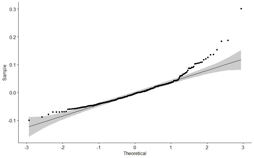
Then 300300 realizations of the random field X⁡(s)X(s) in the square region □(300)={(s1,s2):|si|≤300,i=1,2}\square(300)=\{(s_{1},s_{2}):|s_{i}|\leq 300,i=1,2\} were generated. A realization of the random fields X⁡(s)X(s) in the square □⁡(300)\square(300) on the 2D grid with the step h=0.25h=0.25 and the corresponding values of ξ⁡(μ)\xi(\mu) for μ=10,50,100,…,300\mu=10,50,100,...,300 are given in Figure 1. The Q-Q plot of the simulated values of ξ⁡(300)\xi(300) is shown in Figure 2(a). As μ=300\mu=300 is sufficiently large the distribution is close to the asymptotic one. As expected, it is not Gaussian.

Refer to caption
(a) Realization of X⁡(s)X(s)
Refer to caption
(b) Realization of ξ⁡(μ)\xi(\mu)
Figure 1: Realizations of the random field and its integral functional

Using the obtained realizations of X⁡(s),X(s), the random variables ξ⁡(μ)\xi(\mu) were computed for μ=10,50,100,..,300.\mu=10,50,100,..,300. The box plots of the simulated values of ξ⁡(μ)\xi(\mu) are given in Figure 2(b). Table 1 shows the corresponding Root Mean Square Error (RMSE) of ξ⁡(μ)\xi(\mu) for different values of μ.\mu. Figure 2(b) and the table confirm the convergence of ξ⁡(μ)\xi(\mu) to zero when μ\mu increases.

μ\mu 10 50 100 150 200 250 300
RMSE 0.217 0.106 0.079 0.068 0.057 0.052 0.048
Table 1: RMSE of ξ⁡(μ)\xi(\mu).
Refer to caption
(a) QQplot of ξ⁡(300)\xi(300)
Refer to caption
(b) Boxplots of ξ⁡(μ)\xi(\mu)
Figure 2: Empirical distributions of ξ⁡(μ)\xi(\mu)

6 Conclusions and the future studies

The SLLN for random fields with unboundedly increasing variances and covariance functions was obtained. The conditions of the obtained results allow to consider the case of nonlinear transformations of long-range dependent random fields. The results were derived for a very general class of simply connected observation windows Δ.\Delta.

In the future studies, it would be interesting to obtain:

- Laws of Large Numbers with the complete convergence, see Hu et al. 2012, for multidimensional functional data;

- Necessary and sufficient conditions for the SLLN for non-homogeneous and non-isotropic random fields Gaposhkin 1977;

- Rate of convergence in the SLLN, see Anh et al. 2019; Hu and Sun 2020.

Acknowledgements

The authors would like to thank the anonymous reviewers for their suggestions that helped to improve the style of the paper.

Funding

This research was supported under La Trobe University SEMS CaRE Grant ”Asymptotic analysis for point and interval estimation in some statistical models”. The research of the last listed author was partially funded by the subsidy allocated to Kazan Federal University for the state assignment in the sphere of scientific activities, project 1.13556.2019/ 13.1.

References

  • Alodat and Olenko (2020) Alodat, T. and A. Olenko (2020). On asymptotics of discretized functionals of long-range dependent functional data. To appear in Communications in Statistics - Theory and Methods.
  • Anh et al. (2019) Anh, V., N. Leonenko, A. Olenko, and V. Vaskovych (2019). On rate of convergence in non-central limit theorems. Bernoulli 25(4A), 2920–2948.
  • Ashikhmin et al. (2018) Ashikhmin, A., L. Li, and T. Marzetta (2018). Interference reduction in multi-cell massive MIMO systems with large-scale fading precoding. IEEE Transactions on Information Theory 64(9), 6340–6361.
  • Baron (2014) Baron, M. (2014). Asymptotically pointwise optimal change detection in multiple channels. Sequential Analysis 33(4), 440–457.
  • Bingham et al. (1989) Bingham, N., C. Goldie, and J. Teugels (1989). Regular variation. Cambridge University Press.
  • Cousido-Rocha et al. (2019) Cousido-Rocha, M., J. de Uña Álvarez, and J. Hart (2019). A two-sample test for the equality of univariate marginal distributions for high-dimensional data. Journal of Multivariate Analysis 174, 104537.
  • Gaposhkin (1977) Gaposhkin, V. (1977). Criteria for the strong law of large numbers for classes of stationary and homogeneous random fields. Theory of Probability and its Applications 22(2), 286–310.
  • Hojjatinia et al. (2020) Hojjatinia, S., C. Lagoa, and F. Dabbene (2020). Identification of switched autoregressive exogenous systems from large noisy datasets. To appear in International Journal of Robust and Nonlinear Control.
  • Hu et al. (2005) Hu, T., A. Rosalsky, and A. Volodin (2005). On the golden ratio, strong law, and first passage problem. Mathematical Scientist 30(2), 77–86.
  • Hu et al. (2008) Hu, T., A. Rosalsky, and A. Volodin (2008). On convergence properties of sums of dependent random variables under second moment and covariance restrictions. Statistics & Probability Letters 78(14), 1999–2005.
  • Hu et al. (2012) Hu, T., A. Rosalsky, and A. Volodin (2012). A complete convergence theorem for row sums from arrays of rowwise independent random elements in Rademacher type pp Banach spaces. Stochastic Analysis and Applications 30(2), 343–353.
  • Hu and Sun (2020) Hu, Z. and W. Sun (2020). Convergence rates in the law of large numbers and new kinds of convergence of random variables. To appear in Communications in Statistics - Theory and Methods.
  • Ivanov and Leonenko (2012) Ivanov, A. and N. Leonenko (2012). Statistical analysis of random fields. Springer.
  • Kumar et al. (2019) Kumar, R., M. Wenzel, M. Ellis, M. ElBsat, K. Drees, and V. Zavala (2019). Hierarchical MPC schemes for periodic systems using stochastic programming. Automatica Journal of IFAC 107, 306–316.
  • Li et al. (2017) Li, D., M. Mukhopadhyay, and D. Dunson (2017). Efficient manifold and subspace approximations with spherelets. arXiv preprint arXiv:1706.08263.
  • Lyons (1988) Lyons, R. (1988). Strong laws of large numbers for weakly correlated random variables. Michigan Mathematical Journal 35(3), 353–359.
  • Móricz (1977) Móricz, F. (1977). The strong laws of large numbers for quasi-stationary sequences. Zeitschrift für Wahrscheinlichkeitstheorie und Verwandte Gebiete 38(3), 223–236.
  • Móricz (1985) Móricz, F. (1985). Slln and convergence rates for nearly orthogonal sequences of random variables. Proceedings of the American Mathematical Society 95(2), 287–294.
  • Parker and Rosalsky (2019) Parker, R. and A. Rosalsky (2019). Strong laws of large numbers for double sums of Banach space valued random elements. Acta Mathematica Sinica(English Series) 35(5), 583–596.
  • Pumi et al. (2020) Pumi, G., P. Schaedler, and R. Souza (2020). A dynamic model for double bounded time series with chaotic driven conditional averages. To appear in Scandinavian Journal of Statistics.
  • Serfling (1970) Serfling, R. (1970). Convergence properties of SnS_{n} under moment restrictions. The Annals of Mathematical Statistics 41(4), 1235–1248.
  • Shu and Nan (2019) Shu, H. and B. Nan (2019). Estimation of large covariance and precision matrices from temporally dependent observations. The Annals of Statistics 47(3), 1321–1350.
  • Vega and Rey (2013) Vega, L. and H. Rey (2013). A Rapid Introduction to Adaptive Filtering. Springer.