A Jordan Curve that cannot be Crossed by Rectifiable Arcs on a set of Zero Length

A Jordan curve is an injective image of the unit circle in the plane. The Jordan Curve Theorem asserts that a Jordan curve separates the plane into exactly two complementary components, a bounded interior component and an unbounded exterior component. This gives Jordan curves rather simple topology, but their geometry can be exotic. We say an arc crosses a Jordan curve $\Gamma$ if its endpoints belong in different complementary components of $\Gamma$. Let $H^{1}$ denote the Hausdorff $1$-measure. In this paper, we prove the following theorem, answering a question posed by Sauter in [Sau18].

We would like to make some more general remarks about Theorem 1.1. It is a straightforward calculation from the construction that $\Gamma$ will have positive area, but a simple argument using Fubini’s theorem and integrating over a family of line segments shows that any $\Gamma$ satisfying the conclusion of Theorem 1.1 must have positive area.

By the Riemann mapping theorem and Caratheodory’s theorem, any Jordan curve can be crossed by an arc of $\sigma$-finite length that intersects the Jordan curve at exactly one point. Such an arc is analytic everywhere except possibly at the point where it crosses the boundary. In this sense, the hypothesis of rectifiablility is the weakest hypothesis on $\sigma$ so that the conclusion of Theorem 1.1 will hold.

Theorem 1.1 has been addressed in other contexts, both in the class of arcs $\sigma$ considered and the size of the intersection of $\sigma\cap\Gamma$. Examples of Jordan curves $\Gamma$ that cannot be crossed by line segments at only one point seem well known, see for example [Pet]. In [Bis], Bishop constructs a Jordan curve so that if $\sigma$ is a line segment crossing $\Gamma$, the Hausdorff dimension of $\sigma\cap\Gamma$ is $1$, but the case of positive length is not addressed. Motivated by questions about ordinary differential equations, in [PW12], Pugh and Wu show that Jordan curves that cannot be crossed by rectifiable arcs at exactly one point exist and are actually generic (in a Baire sense) in the space of Jordan curves in the plane (equipped with an appropriate metric).

The curve $\Gamma$ also has connections to conformal welding. If $\Gamma$ is a Jordan curve in the plane, let $\Omega$ denote its bounded complementary component. Then there are conformal mappings $f:\mathbb{D}\rightarrow\Omega$ and $g:\mathbb{C}\setminus\overline{\mathbb{D}}\rightarrow\mathbb{C}\setminus\overline{\Omega}$ which induce a circle homeomorphism $h:g\circ f^{-1}:\partial\mathbb{D}\rightarrow\partial\mathbb{D}$ which we call a conformal welding. $\Gamma$ is called log-singular if there is a Borel set $E$ so that $E$ and $h(S^{1}\setminus E)$ both have zero logarithmic capacity (for the definition of logarithmic capacity, see Chapter III of [GM05]). Results of Buerling in [Beu40] show that if $\varphi:\mathbb{D}\rightarrow\Omega$ is a conformal mapping onto a Jordan domain $\Omega$, and $\zeta\in S^{1}$.

except perhaps on a set of zero logarithmic capacity (see also 23(a), p. 127, in [GM05]). It follows that outside of this exceptional set, the image of the hyperbolic geodesic rays $[0,\zeta)$ have finite length. Applying this result to both $f$ and $g$, it follows from Theorem 1.1 that $\Gamma$ is log-singular. Otherwise, by using a pair of two finite length geodesics with the same endpoint on $\Gamma$, we could construct a finite length arc crossing $\Gamma$ at exactly one point. Our example gives the first explicit construction of a log singular curve. For more on log-singular curves and conformal welding, see [Bis94] and [Bis07].

We will construct the curve $\Gamma=\bigcap_{n=1}^{\infty}\Gamma_{n}$ in Theorem 1.1 as a nested intersection of axis aligned tubes which we call plumbings. Given a plumbing, we will use a Lakes of Wada type of construction to construct a new plumbing which weaves back and forth inside of itself, see Figure 1. For a rectifiable curve $\sigma$ that passes from the interior boundary component to the exterior boundary component of $\Gamma$, we let $l_{n}=H^{1}(\Gamma_{n}\cap\sigma).$ In order for $l_{n+1}$ to be much smaller than $l_{n}$, $\sigma$ must weave back and forth horizontally so that it can pass through the vertical gaps, as seen in Figure 1. We will tune the parameters defining the plumbings $\Gamma_{n}$ so that $\sigma$ can only pass through a increasingly smaller percentage of the vertical gaps of $\Gamma_{n}$ as $n\rightarrow\infty$. It will follow that most of the time, the connected components of $\sigma\cap\Gamma_{n+1}$ must pass through those components approximately as a straight line segment, and we will show directly that a straight line segment intersects $\Gamma$ with a set of positive length. These observations combined will allow us to prove Theorem 1.1.

The structure of the paper is as follows. In Section 2, we define all the necessary terminology and reduce Theorem $1.1$ to the case of rectifiable curves with length $1$. In Section $3$, we carefully define plumbings and discuss their properties. In Sections 4 and 5, we show how to create new plumbings from old to create the limiting Jordan curve $\Gamma$. In Section 6, we show that the Jordan curve cannot be crossed at a single point by rectifiable curves, and in Section 7 we refine this to show the intersection of the rectifiable curve with the Jordan curve has positive area.

A curve is a continuous function $\sigma:[0,1]\rightarrow\mathbb{C}$. If $\sigma$ is a curve with $\sigma(0)=\sigma(1)$ we call $\sigma$ closed. We will sometimes refer to curves that are not closed as arcs. A curve $\sigma$ is called simple if for all $t_{1}\neq t_{2}\in[0,1]$, we have $\sigma(t_{1})\neq\sigma(t_{2})$. Similarly, we call a closed curve simple if for all $t_{1}\neq t_{2}\in[0,1)$, we have $\sigma(t_{1})\neq\sigma(t_{2})$. A Jordan curve is a simple closed curve. The image $\sigma([0,1])\subset\mathbb{C}$ is the trace of $\sigma$. When it will not cause confusion, we will refer the trace of a curve $\sigma$ and the curve $\sigma$ interchangeably. Recall that the length of a curve $\sigma$ is defined to be

If $l(\sigma)<\infty$, we call the curve or arc $\sigma$ rectifiable.

If $\sigma$ crosses $\Gamma$, we are interested in the subset of points where $\sigma$ passes from one complimentary component of $\Gamma$ to the other.

The definition of pierceability can be easily adjusted to include other families of curves, such as line segments, simple rectifiable curves, and rectifiable curves of some given length. If $\Gamma$ is unpierceable by rectifiable curves, the piercing set is nontrivial.

In fact, it is not difficult to see additionally that $\mathcal{P}(\sigma)$ is a Cantor set: compact, uncountable, totally disconnected, and no isolated points.

The curve $\Gamma$ we construct will be the nested intersection of a sequence of topological annuli which we call plumbings. We first define the two basic pieces that determine a plumbing. See Figure 2.

To form a straight piece, start with a rectangle with sides parallel to the coordinate axes, and remove two of the opposite sides. We call the remaining sides the boundary sides of the straight piece and the sides we removed the openings of the straight piece. We call the boundary side that is a subset of the interior boundary component of the plumbing the top of the straight piece, and the boundary side which is a subset of the exterior boundary component of the plumbing the bottom of the straight piece. Whenever we need to analyze a specific straight piece, we will orient our point of view to justify these names.

Corner pieces are formed by taking an axis aligned rectangle and removing two adjacent sides, but keeping the mutual vertex of the two removed sides. This vertex is called an inner corner for the corner piece, and the remaining sides are similarly called boundary sides and openings. Plumbings are formed by alternating straight and corner pieces and gluing together their openings by arc length. See Figure 3 for an example of a plumbing.

We define the following geometric quantities associated to a plumbing. The width of a straight piece is defined to be the distance between its boundary sides. The width of a plumbing is defined to be the maximum of the widths of the straight pieces in the plumbing. The length of a straight piece is the distance between its openings. The min-length of a plumbing is the minimum of the lengths of its straight pieces.

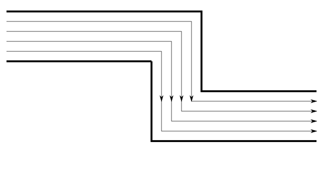
Plumbings come with a natural foliation of axis aligned polygonal curves that follow the inner and outermost boundary. Start with a plumbing $P$, and let $\gamma_{0}$ and $\gamma_{1}$ denote the outermost and innermost boundary components, respectively. Decompose $P$ into its straight and corner pieces. Given a straight piece $S$ and a number $t\in(0,1)$, let $w$ denote its width. Let $s_{t}$ denote the line segment parallel to the boundary sides of $S$ with distance $t\cdot w$ from $\gamma_{0}$. Draw this line segment for all straight pieces in $P$. Any corner piece is adjacent to two straight pieces, and each of its openings contains an endpoint of some $s_{t}$ and some $s_{t}^{\prime}$. Continue the segments $s_{t}$ and $s_{t}^{\prime}$ until they intersect (this point of intersection will be on the diagonal that separates the openings of the corner piece) and repeat this for all corner pieces to form a Jordan curve $\gamma_{t}$. We define $\gamma_{1/2}$ to be the core curve of $P$. We call $\{\gamma_{t}\}$ the plumbing foliation of $P$. Whenever we parameterize the elements of a plumbing foliation, we do so counterclockwise, so that the inner boundary component is always to the left of the curve in the foliation. See Figure 4.

.

A point on the core curve of $P$ where the core curve changes from a vertical segment to a horizontal segment or vice versa is called a bend point. Two bend points are called adjacent if there is no bend point between them. Every bend point is adjacent to exactly two other bend points. Let $z$ and $w$ be two adjacent bend points of $P$, so that the core curve passes through $z$ first. The $(z,w)$-junction is the union of the two corner pieces containing $z$ and $w$, and the straight piece that is between $z$ and $w$. Each $(z,w)$ junction takes two possible forms, depending on how the openings of the corner pieces are configured. We call the junctions $U$-junctions and $Z$-junctions, respectively. When considered with respect to the orientation of the core curve, there are four junctions to consider. See Figure 6.

In this section we define a procedure which takes a plumbing $\Gamma_{n}$ and creates a plumbing $\Gamma_{n+1}$ contained inside of $\Gamma_{n}$ taking up most of the area of $\Gamma_{n}$, but having a much smaller width. Roughly put, we will insert very thin vertical and horizontal rectangles segments inside of $\Gamma_{n}$ to form a new plumbing. This procedure will form the basis of our construction.

Let $\Gamma_{n}$ be a plumbing. Define

where $l_{n}$ is the min-length of $\Gamma_{n}$ and $w_{n}$ is the width of $\Gamma_{n}$. Subdivide $\Gamma_{n}$ into straight pieces and corner pieces, and denote the plumbing foliation of $\Gamma_{n}$ by $\{\gamma^{n}_{t}\}$. Parameterize $\gamma^{n}_{1/2}$ as a Jordan curve, say, by arc length. Denote $P_{0}$ as the unique plumbing piece of $\Gamma_{n}$ so that $\gamma^{n}_{1/2}(0)\in P_{0}$ and so that there exists $\delta>0$ so that $\gamma^{n}_{1/2}:[0,\delta)\rightarrow P_{0}$. Label the rest of the plumbing pieces $\{P_{i}\}_{i=0}^{m-1}$ according to the order $\gamma^{n}_{1/2}(t)$ passes through them. We will consider this list of pieces modulo $m$, so that $P_{m}=P_{0}$.

Choose some $\delta_{n}\in(0,1/100)$. We are going to subdivide the straight pieces $P_{i}$ further into rectangles by connecting the boundary sides by line segments placed distance approximately $\delta_{n}d_{n}$ apart; no line segment will be farther than $2\delta_{n}d_{n}$ from the adjacent line segments we place, and no line segment will be closer than $1/2\delta_{n}d_{n}$ from the adjacent line segments we place. We will simply refer to these new rectangles as subdivided rectangles. If $P_{i}$ is the straight piece of a $U$-junction, we must make sure that the number of subdivide rectangles of $P_{i}$ is even. If $P_{i}$ is an element of a $Z$-junction, the number of subdivided rectangles should be odd. See Figure 7.

Given any $t_{n}\in\mathbb{N}$, we select the elements of the plumbing foliation $\{\gamma^{n}_{j/t_{n}}\}_{j=0}^{t_{n}}.$ We will always assume that $t_{n}$ is an odd number, so that we are selecting $t_{n}+1$ equally spaced elements of the foliation. If $w_{n}$ is the width of $\Gamma_{n}$, then adjacent elements of the plumbing foliation inside of a straight piece are no more than distance $\frac{w_{n}}{t_{n}}$ apart.

For each straight piece $P_{i}$, we want to assign a labels $T$ and $B$ for its subdivided rectangles.

1. (1)

   If $P_{i-1}$’s boundary side extends the bottom boundary side of $P_{i}$, the first subdivided rectangle is marked as T.

2. (2)

   If $P_{i-1}$’s boundary side extends the upper boundary side of $P_{i}$, the first subdivided rectangle is marked as B.

We alternate T and B until we reach the end of the straight piece.

Given a straight piece $P$, we have $P=\cup R_{i}$, where $R_{i}$ are the subdivided rectangles of $P$ described above with base approximately $\delta_{n}d_{n}$ and with height no greater than $w_{n}$. Choose some positive integer $v_{n}=k^{2}$ for some $k\geq 3$ and then choose some subdivided rectangle $R_{i}$. Decompose the base of $R_{i}$ into $v_{n}$ many equal length segments. We will need the following definition and combinatorial fact.

The following lemma is simple, and we leave its proof to the reader, with Figure 8 as a hint. A rook placement satisfying the conditions of Lemma 4.2 is called a good $v_{n}$-rook placement.

Supose that $R_{i}$ is a subdivided rectangle of some straight piece, and that $R_{i}$ is designated as T. The plumbing foliation cuts $R_{i}$ into $t_{n}$ many rectangles. Orienting our point of view and counting downwards from the boundary side intersecting the interior complementary component, we call the first $2v_{n}$ many rectangles a $v_{n}$-slab inside $R_{i}$. A $v_{n}$-slab decomposes into a $v_{n}$ by $v_{n}$ grid. Rows are determined by every two elements of the plumbing foliation, and the columns are determined by the $v_{n}$ equally spaced points on the base of $R_{i}$. We choose a good $v_{n}$-rook placement for this grid. For each rook in this good $v_{n}$-rook placement, place a vertical line segment connecting the top and bottom of the rook through the middle. This segment has endpoints on two elements of the plumbing foliation for $\Gamma_{n}$ that determine the rows, and passes through exactly one foliation element between the two. See Figure 9.

We can split the rest of $R_{i}$ into $v_{n}$ slabs, going from the top down and repeating the rook placement of the top $v_{n}$-slab until we reach the element $\gamma^{n}_{1/t_{n}}$ of the plumbing foliation. We can choose $t_{n}$ to be larger if we need to so that the final $v_{n}$-slab has a bottom side determined by $\gamma^{n}_{1/t_{n}}$; we will always assume that $t_{n}$ satisfies this property.

One $v_{n}$ slab forms a rectangle with base length approximately $\delta_{n}d_{n}$ and height $2v_{n}w_{n}/t_{n}$. In our construction, the height $2v_{n}w_{n}/t_{n}$ will be much smaller than $\delta_{n}d_{n}$. The amount of $v_{n}$ slabs we need to stack to form an approximate $\delta_{n}d_{n}$ by $\delta_{n}d_{n}$ $v_{n}$-square is approximately $k_{n}$, where,

Or,

We also can see that $R_{i}$ decomposes into approximately

many $v_{n}$-squares.

We do the same thing with the rectangles labeled $B$, except instead of building $v_{n}$-slabs starting from the top down, we build $v_{n}$-slabs starting from the bottom up. We do not place any segments connecting elements of the plumbing foliation in corner pieces.

We now draw line segments along the plumbing foliation. In corner pieces, we add the intersection of all elements in the plumbing foliation with the corner piece. See Figure 10. In straight pieces, we do the same thing, except we remove the portion of the plumbing foliation within distance $w_{n}/t_{n}$ of the center of vertical line segments we placed in the previous step. See Figure 14.

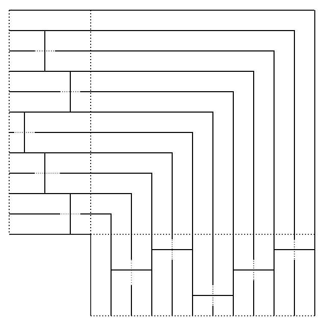
With the procedure above of adding in vertical and horizontal line segments into straight and corner pieces, we have constructed a topological subannulus contained inside of $\Gamma_{n}$. The only issue remaining is that its boundary components are not Jordan curves. To do this, we will thicken all of the segments in the horizontal and vertical directions by a small amount so that the segments we added become rectangles. The amount we thicken is given by

The following theorem is now clear:

The core curve of $\Gamma_{n+1}$ can be visualized in Figure 11.

We now construct the Jordan curve $\Gamma$. Fix $\epsilon_{0}>0$ and let $\Gamma_{0}$ be the topological annulus formed by taking the open square of side length $2(1+\epsilon_{0})$ centered at the origin and removing the closed square of side length $2(1-\epsilon_{0})$ centered at the origin. $\Gamma_{0}$ is a square plumbing, and parameterize its core curve using a constant speed parameterization. Using the procedure in the previous section, we construct a plumbing with the following parameters. At each stage $n$, we must choose a parameter $v_{n}$. We assume that $v_{n}$ is strictly increasing, and we always choose $v_{n}$ to be a perfect square. Moreover, we will demand that

We will always assume that the parameters $\delta_{n}$ satisfy

Notice that for any valid choice of $t_{n}$, the widths $w_{n}$ will always satisfy the inequality

Given these above quantities, we will always choose $t_{n}$ large enough so that it satisfies

By (5.1) and (5.4) we know that

From this it easily follows that

In this section, we will prove the following:

To prove this, the first step is to construct appropriate parameterizations of $\gamma^{n+1}_{1/2}$ given some parameterization of the core curves $\gamma^{n}_{1/2}$ of $\Gamma_{n}$. Since we will always work with the core curves in this section, we will call $\gamma^{n}_{1/2}:=\gamma^{n}$.

Recall that each straight piece $P$ of $\Gamma_{n}$ is decomposed into subdivided rectangles with base approximately $\delta_{n}d_{n}$ and height $w_{n}$. We do not decompose the corner pieces and leave them as is. For some small choice of $\delta$, $\gamma^{n}(0,\delta)$ is contained in one of these subdivided rectangles or corners, so we denote it as $R_{0}$. We label the rest of the subdivided rectangles and corner pieces in the order that $\gamma^{n}$ passes through them. This gives a list of subdivided rectangles and corners $\{R_{i}\}_{i=0}^{m-1}$. We will consider this list modulo $m$, so that $R_{0}=R_{m}$. Let and $t_{i}\in[0,1]$ for $i=1,\dots m$ be the first entry time of $\gamma^{n}$ in $R_{i}$. $t_{m}$ will be the exit time for $R_{m-1}$, which coincides with entering back inside $R_{0}$. $\gamma^{n}:(t_{m},1]\cup[0,t_{1})$ goes from the end of $R_{m-1}$ to the end of $R_{0}$.

We’ll show how to parameterize $\gamma^{n+1}$ inside of the intervals $(t_{i},t_{i+1})$. Here we take the convention that $(t_{m},t_{m+1})=(t_{m},1]\cup[0,t_{1})$. To do this, we will show where to place the points $\gamma^{n+1}(t_{i})$ and $\gamma^{n+1}(t_{i+1})$. Then for the subarc of $\gamma^{n+1}$ in between these points, we will use a constant speed parameterization. We will handle this with three cases.

For the first case, suppose that $R_{i}$ is a subdivided rectangle of a straight piece so that $R_{i+1}$ is not a corner piece. Orient $R_{i}$ so that the top boundary side is a subset of the innermost boundary component of $\Gamma_{n}$. If $R_{i}$ was labeled as B, then $\gamma^{n+1}(t_{i})$ will be the point on the intersection of $\gamma^{n+1}$ and the left side of $R_{i}$ between $\gamma^{n}_{\frac{t_{n}-1}{t_{n}}}$ and $\gamma^{n}_{1}$. We let $\gamma^{n+1}_{1/2}(t_{i+1})$ be the point on the intersection of $\gamma^{n+1}$ and the right side of $R_{i}$ between $\gamma^{n}_{\frac{1}{t_{n}}}$ and $\gamma^{n}_{0}$. If $R_{i}$ was labeled as T, we do the opposite. $\gamma^{n+1}(t_{i})$ will be the point on the intersection of $\gamma^{n+1}$ and the left side of $R_{i}$ between and $\gamma^{n}_{\frac{1}{t_{n}}}$ and $\gamma^{n}_{0}$, and $\gamma^{n+1}(t_{i+1})$ will be be the point on the intersection of $\gamma^{n+1}$ and the left side of $R_{i}$ between $\gamma^{n}_{\frac{t_{n}-1}{t_{n}}}$ and $\gamma^{n}_{1}$. See Figure 12.

Suppose that $R_{i}$ is a subdivided rectangle so that $R_{i+1}$ is a corner boundary piece. Then we label $\gamma^{n+1}(t_{i})$ using the procedure above. We let $\gamma^{n+1}(t_{i+1})$ be the point in the same straight piece as $\gamma^{n+1}(t_{i})$ that lies on the right side of $R_{i}$. See Figure 13.

Finally, suppose that $R_{i}$ is a corner piece. Then $R_{i-1}$ and $R_{i+1}$ fall into the above cases, which means that $\gamma^{n+1}(t_{i})$ and $\gamma^{n+1}(t_{i+1})$ have already been defined. The former corresponds to the first time that $\gamma^{n+1}$ enters the corner piece, and the latter corresponds to the last time $\gamma^{n+1}$ exits the corner piece. We again use the constant speed parameterization to parameterize the subarc between these two points. See Figure 13.

It follows that $\gamma^{n}$ converges uniformly to $\gamma$ for some continuous function $\gamma:[0,1]\rightarrow\mathbb{C}$. Since $\gamma$ is continuous and the widths of $\Gamma_{n}$ are strictly decreasing, we must have $\gamma([0,1])=\Gamma$. So to show $\Gamma$ is a Jordan curve it is sufficient to show that $\gamma$ is injective.

By Lemma 2.3, to show that $\Gamma$ is non-pierceable by rectifiable arcs, we only must prove that $\Gamma$ is not pierceable by unit length simple rectifiable curves which cross $\Gamma$.

We will always parameterize $\sigma$ crossing $\Gamma$ so that $\sigma(0)$ is in the bounded complementary component of $\Gamma$. The following lemma is easy to visualize, but its proof is cumbersome. The idea is that if $\sigma$ has endpoints in distinct complementary components of $\Gamma_{n}$, to cross $\Gamma$ at exactly one point, $\sigma$ is forced to remain in the part of $\Gamma_{n}$ we removed to construct $\Gamma_{n+1}$, otherwise it will cross more than once. Therefore, such a $\sigma$ must remain inside of one subdivided rectangle of $\Gamma_{n}$, so that it must completely cross a $v_{n}$-slab. See Figure 12 and Figure 14.

The statement and proof of Lemma 6.2 apply in exactly the same way if $v_{n}$-slabs are replaced by $v_{n}$-squares, since equation $(\ref{deltan})$ implies that $\lambda_{n}$, the number of $v_{n}$-squares contained inside of a subdivided rectangle, also tends to $\infty$ as $n\rightarrow\infty$. This means we may assume there are many $v_{n}$-squares in the bounded and unbounded complementary components of the core curve of $\Gamma_{n}$, and the reasoning of the proof still applies.

In fact, since the number of $v_{n}$-slabs and $v_{n}$-squares tends to $\infty$, for large enough $n$, the reasoning of Lemma 6.2 allows us to conclude that there are at least three adjacent $v_{n}$-slabs or $v_{n}$-squares so that $\sigma$ enters ever single rook of all three $v_{n}$-slabs or $v_{n}$-squares. We will use this observation in the basic estimates below.

We would like to focus on a convenient subarc of $\sigma$, which exists by the following lemma.

We will show that the subarc that begins at the top of a straight piece and exits at the bottom of a straight piece intersects with positive length. We first consider the special case that this subarc is a line segment.

Recall that we always may orient our view so that that this axis aligned line segment is vertical.

With a little more care, we can upgrade these observations above to the proof of Theorem 1.1.

If $\sigma$ intersects a thickened line segment in some rook, we will just assume that $\sigma$ passed through the thickened line segment. This causes $l_{n+1}$ to decrease, but fortunately this cannot happen often. Indeed, note that $2k_{n}v_{n}$, is a very small percentage of $t_{n}$, since by $(\ref{kn})$,

References

- [Beu40] Arne Beurling. Ensembles exceptionnels. Acta Math., 72:1–13, 1940.
- [Bis] Christopher J. Bishop. A curve with no simple crossings by segments. Preprint:.
- [Bis94] Christopher J. Bishop. Some homeomorphisms of the sphere conformal off a curve. Ann. Acad. Sci. Fenn. Ser. A I Math., 19(2):323–338, 1994.
- [Bis07] Christopher J. Bishop. Conformal welding and Koebe’s theorem. Ann. of Math. (2), 166(3):613–656, 2007.
- [GM05] John B. Garnett and Donald E. Marshall. Harmonic measure, volume 2 of New Mathematical Monographs. Cambridge University Press, Cambridge, 2005.
- [Pet] Anton Petrunin. Answer to: https://mathoverflow.net/questions/100025/how-many-times-line-segments-can-intersect-a-jordan-curve/100035.
- [PW12] Charles Pugh and Conan Wu. Jordan curves and funnel sections. J. Differential Equations, 253(1):225–243, 2012.
- [Sau18] Manfred Sauter. How twisted can a Jordan curve be? In Ulmer Seminare 2016/2017, Funktionalanalysis und Differentialgleichungen, Abschlussband mit Dreizeilenbeweisen und offenen Problemen, volume 20 of Ulmer Seminare, pages 133–140. Institute of Applied Analysis, Ulm University, 2018.