Improving Neural Network Training in Low Dimensional Random Bases
Abstract
Stochastic Gradient Descent (SGD) has proven to be remarkably effective in optimizing deep neural networks that employ ever-larger numbers of parameters. Yet, improving the efficiency of large-scale optimization remains a vital and highly active area of research. Recent work has shown that deep neural networks can be optimized in randomly-projected subspaces of much smaller dimensionality than their native parameter space. While such training is promising for more efficient and scalable optimization schemes, its practical application is limited by inferior optimization performance.
Here, we improve on recent random subspace approaches as follows: Firstly, we show that keeping the random projection fixed throughout training is detrimental to optimization. We propose re-drawing the random subspace at each step, which yields significantly better performance. We realize further improvements by applying independent projections to different parts of the network, making the approximation more efficient as network dimensionality grows. To implement these experiments, we leverage hardware-accelerated pseudo-random number generation to construct the random projections on-demand at every optimization step, allowing us to distribute the computation of independent random directions across multiple workers with shared random seeds. This yields significant reductions in memory and is up to 10 faster for the workloads in question.
1 Introduction
Despite significant growth in the number of parameters used in deep learning networks, Stochastic Gradient Descent (SGD) continues to be remarkably effective at finding minima of the highly over-parameterized weight space [9]. However, empirical evidence suggests that not all of the gradient directions are required to sustain effective optimization and that the descent may happen in much smaller subspaces [14]. Many methods are able to greatly reduce model redundancy while achieving high task performance at a lower computational cost [34, 29, 5, 36, 17, 15, 32, 21].
Notably, Li et al. [26] proposed a simple approach to both quantify and drastically reduce parameter redundancy by constraining the optimization to a (fixed) randomly-projected subspace of much smaller dimensionality than the native parameter space. While the work demonstrated successful low-dimensional optimization, its inferior performance compared with standard SGD limits its practical application.
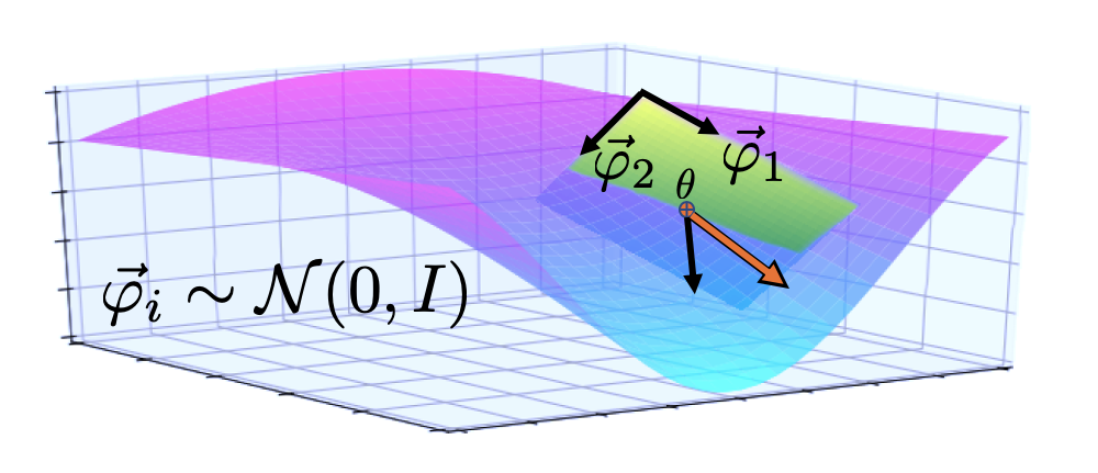
Here, we revisit optimization in low-dimensional random subspaces with the aim of improving its practical optimization performance. We show that while random subspace projections have computational benefits such as easy distribution on many workers, they become less efficient with growing projection dimensionality, or if the subspace projection is fixed throughout training. We observe that applying smaller independent random projections to different parts of the network and re-drawing them at every step significantly improves the obtained accuracy on fully-connected and several convolutional architectures, including ResNets on the MNIST, Fashion-MNIST and CIFAR-10 datasets.11 1 Our source code is available at https://github.com/graphcore-research/random-bases
2 Background
Using random projections to reduce dimensionality is appealing both computationally (fewer dimensions to operate on) and theoretically (due to their well-known approximation capabilities [20, 31, 13]). Sampled projections can map from sufficiently high-dimensional into low-dimensional Euclidean spaces without affecting the relative distances in a point sample. Thus, they can make investigations of certain complex structures more tractable [8]. Furthermore, they are computationally cheap to generate and can be easily stored, communicated, and re-created using random seeds [33].
2.1 Random projections for neural network optimization
Li et al. [26] utilized random projections to reduce the dimensionality of neural networks, aiming to quantify the difficulty of different tasks. Specifically, they constrained the network optimization into a fixed low-dimensional, randomly oriented hyper-plane to investigate how many dimensions are needed to reach 90% accuracy against the SGD baseline on a given task (Fixed Projection Descent, FPD). They found that this “intrinsic dimensionality” tended to be much lower than the parameter dimensionality of the network, suggesting that the network’s solution space of the problem was smaller than its parameterization implied. Since FPD performs the parameter update in the fixed low-dimensional subspace (not native parameter space), the amount of trainable parameters is reduced significantly. However, the optimization progress is only defined with respect to the particular projection matrix and constrained to the subspace sampled at initialization.
2.2 Random projections for derivative-free gradient approximation
As opposed to using the analytical gradient of the loss with respect to sampled subspaces, random directions also allow for stochastic gradient-free estimation [30, 23, 4, 37]. Notably, variants of the derivative-free Natural Evolution Strategies (NES) have recently been applied to train large-scale image classification and reinforcement learning policy networks with hundreds of thousands of dimensions, suggesting that low-dimensional random directions may be rich enough to capture gradient information of high-dimensional neural networks [33, 25]. We discuss the formal connection of our approach with ES in Section A of the Supplementary Material.
2.3 Random projections for analysis of the loss landscape
Another application area of dimensionality reduction through random projection is the analysis of the neural network loss landscape. In its simplest form, the loss surface can be projected onto linear subspace by evaluating a number of loss values in random directions. Li et al. [27] conducted a comprehensive visualization of the loss landscapes for various architecture choices. They observed a transition from smooth to highly chaotic surfaces with increasing network depth. He et al. [18] analyzed the low-loss regions in “asymmetric” random directions to argue that the location of a solution within a valley correlates with its generalization ability. Random projection can also make computationally prohibitive forms of analysis more feasible. For instance, [11] computed and analyzed the Hessian of lower-dimensional random hyperplanes of neural networks to investigate the relation of local curvature and the effectiveness of a given initialization. In follow-up work, [10] proposed a model of a neural network’s local geometry. As we will discuss in Section 4.5, our method allows for visualizations of the loss surface in the sampled random directions at every step to analyze the descent behavior.
2.4 Scalability and parallelization of random projections
Network training often leverages parallel computation of stochastic gradients on different workers that are exchanged and averaged at every step (data parallel SGD). However, inter-worker communication to exchange the locally-computed -dimensional gradients can become a prohibitive bottleneck for practical distributed implementations [2, 36]. Notably, optimization in random subspaces can make the parallel execution on many workers more efficient, since random vectors are computationally cheap to generate and can be shared by the workers before the start of the training as a sequence of random seeds [33]. The locally-computed gradient can thus be communicated using only the low-dimensional gradient vector, while the high-dimensional update can be regenerated using the random projection. Our approach actively leverages this property to enable an efficient implementation of large random projections.
3 Method
In this section, we formally propose our method for low-dimensional optimization in random bases. We consider the following setting: Given a data distribution from which samples are drawn, we seek to learn the parameters of a neural network by minimizing the empirical risk of the form , where denotes the network’s loss on the samples of the training set of size .
SGD optimizes the model using a stochastic gradient where are randomly drawn samples of at timestep . The weights are adjusted iteratively following the update equation with learning rate . In the commonly used mini-batch version of SGD, the update gradient is formed as an average of gradients over a mini-batch sample of size . To simplify the discussion, we have omitted the explicit notation of the mini-batch in the following gradient expressions.
3.1 Random bases descent
To reduce the network training dimensionality, we seek to project into a lower dimensional random subspace by applying a random projection matrix to the parameters , where denotes the network’s initialization and the low-dimensional trainable parameter vector of size with . If ’s column vectors are orthogonal and normalized, they form a randomly oriented base and can be interpreted as coordinates in the subspace. As such, the construction can be used to train in a -dimensional subspace of the network’s original -dimensional parameter space.
In this formulation, however, any optimization progress is constrained to the particular subspace that is determined by the network initialization and the projection matrix. To obtain a more general expression of subspace optimization, the random projection can instead be formulated as a constraint of the gradient descent in the original weight space. The constraint requires the gradient to be expressed in the random base with random basis vectors and coordinates . The gradient step can be directly used for descent in the native weight space following the standard update equation .
To obtain the -dimensional coordinate vector, we redefine the training objective itself to implement the random bases constraint:
Computing the gradient of this modified objective with respect to at and substituting it back into the basis yields a descent gradient that is restricted to the specified set of basis vectors:
.
The resulting optimization method is given in Algorithm 1. Note that this scheme never explicitly calculates a gradient with respect to , but performs the weight update using only the coordinate gradients in the respective base.
| Random Bases Descent (RBD) Algorithm | Parallelized RBD |
|---|---|
| Input: Learning rate , network initialization | Input: Learning rate , network initialization |
| Initialize: workers with known random seeds | |
| for | for |
| for each worker | |
| Sample random base | Sample random base |
| Reset coordinates to | Reset coordinates to |
| Compute coordinates | Compute coordinates |
| end for | |
| Send all coordinates from each worker to every other worker | |
| for each worker | |
| Reconstruct random bases for | |
| Update weights | Update weights |
| end for | |
| end for | end for |
3.1.1 Compartmentalized approximation
The gradient expression allows not only for the adjustment of the basis vectors at different steps (time axis), but can also be partitioned across the -dimensional parameter space (network axis). Such partitioning of the network into different compartments can improve the approximation capability of the subspace. Consider approximating a -dimensional vector in a random base with bounded coefficients: . As the dimensionality of grows, it may be required to generate exponentially many samples as the independently chosen random basis vectors become almost orthogonal with high probability [8]. For high-dimensional network architectures, it can thus be useful to reduce the approximation dimensionality through compartmentalization of the approximation target (the network parameters). For instance, could be partitioned into evenly sized compartments of dimension . The compartments would be approximated with independent bases of reduced dimensionality: While the overall number of coefficients and bases vectors remains unchanged, partitioning the space constrains the dimensionality of randomization, which can make random approximation much more efficient [13]. It can be instructive to consider extreme cases of compartmentalized approximations. If the , we recover the SGD gradient as every weight forms its own compartment with a trainable coefficient. If and is large enough to form an orthogonal base, the optimization becomes a randomly rotated version of SGD. Apart from evenly dividing the parameters, we construct compartmentalization schemes more closely related to the network architecture. For example, we use “layer-wise compartmentalization”, where the parameter vector of each layer uses independent bases. The bases dimension in each compartment can also be adjusted dynamically based on the number of parameters in the compartment. If the number and dimension of the compartments are chosen appropriately, the total amount of trainable coefficients can be kept low compared to the network dimensionality.
4 Results and discussion
4.1 Experimental setup
The architectures we use in our experiments are: a fully-connected (FC) network, a convolutional neural network (CNN), and a residual network (ResNet) [19]. Since we have to generate random vectors of the network size in every training step, for initial evaluation, we choose architectures with a moderate () number of parameters. All networks use ReLU nonlinearities and are trained with a softmax cross-entropy loss on the image classification tasks MNIST, Fashion-MNIST (FMNIST), and CIFAR-10. Unless otherwise noted, basis vectors are drawn from a normal distribution and normalized. We do not explicitly orthogonalize, but rely on the quasi-orthogonality of random directions in high dimensions [13]. Further details can be found in the Supplementary Material.
4.2 Efficient random bases generation
As apparent from Algorithm 1, the implementation depends on an efficient generation of the dimensional random subspace projections that are sampled at each step of the training. To meet the algorithmic demand for fast pseudo-random number generation (PRNG), we conduct these experiments using Graphcore’s first generation Intelligence Processing Unit (IPU)22 2 https://graphcore.ai. The Colossus™ MK1 IPU (GC2) accelerator is composed of 1216 independent cores with in-core PRNG hardware units that can generate up to 944 billion random samples per second [22]. This allows us to generate the necessary random base vectors locally on the processor where the computation happens — substituting fast local compute for expensive communication. The full projection is never kept in memory, but encoded as a sequence of random seeds; samples are generated on demand during the forward-pass and re-generated from the same seed during the backward-pass. Although our TensorFlow implementation did not rely on any hardware-specific optimizations, the use of the hardware-accelerated PRNG proved to be essential for fast experimentation. On a single IPU, random bases descent training of the CIFAR-10 CNN with the extremely sample intensive dimension k achieved a throughput of 31 images per second (100 epochs / 1.88 days), whereas training the same model on an 80 core CPU machine achieved 2.6 images/second (100 epochs / 22.5 days). To rule out the possibility that the measured speedup can be attributed to the forward-backward acceleration only, we also measured the throughput of our implementation on a GPU V100 accelerator but found no significant throughput improvement relative to the CPU baseline.
4.3 Distributed implementation
The training can be accelerated further through parallelization on many workers. Like with SGD, training can be made data parallel, where workers compute gradients on different mini-batches and then average them. RBD can also be parallelized by having different workers compute gradients in different random bases. Gradients can be exchanged using less communication bandwidth than SGD, by communicating the low-dimensional coefficients and the random seed of the base. Notably, the parallelization scheme is not limited to RBD but can also be applied to the fixed random projection methods of [26]. In Figure 5, we investigate whether training performance is affected when distributing RBD. We observe constant training performance and almost linear wall-clock scaling for 16 workers.
4.4 Performance on baseline tasks
| Model | NES | FPD | RBD | SGD |
|---|---|---|---|---|
| FC-MNIST | 22.51.7 (0.23) | 800.4 (0.81) | 93.8930.024 (0.96) | 98.270.09 |
| FC-FMNIST | 456 (0.52) | 77.30.29 (0.89) | 85.650.2 (0.98) | 87.320.21 |
| FC-CIFAR10 | 17.80.5 (0.34) | 21.41.2 (0.41) | 43.770.22 (0.84) | 52.090.22 |
| CNN-MNIST | 516 (0.51) | 88.90.6 (0.89) | 97.170.1 (0.98) | 99.410.09 |
| CNN-FMNIST | 374 (0.4) | 77.81.6 (0.85) | 85.560.1 (0.93) | 91.950.18 |
| CNN-CIFAR10 | 20.31 (0.25) | 37.20.8 (0.46) | 54.640.33 (0.67) | 81.40.4 |
We begin by establishing performance on the fully-connected and convolutional architectures for dimensions, which is the lowest reported intrinsic dimensionality for the image classification problems investigated by Li et al. [26]. Table 1 reports the validation accuracy after 100 epochs (plots in Supplementary Material, Figure B.6). All methods other than SGD use a dimensionality reduction factor of . As expected, SGD achieves the best validation accuracy. The NES method displays high training variance while failing to achieve even modest performance in any task. FPD falls short of the SGD target by percentage points, while exceeding the performance of NES. By changing the basis at each step, RBD manages to decrease the FPD-SGD gap by up to 20%. Just like SGD, the random subspace training shows little variance between independent runs with different initializations.
4.5 Properties of random bases optimization
It is worth noting that FPD tends to converge faster than other methods, but to a lower validation accuracy when compared to RBD. This suggests that fixing the basis is detrimental to learning. Having established baseline performances, we now move onto reducing the remaining performance gap to SGD.
Influence of dimensionality
Intuitively, performance should improve when using a larger number of basis vectors as the subspace descent is able to better approximate the “true” gradient. To analyze this, we follow Zhang et al. [38] in quantifying the similarity of the RBD gradient and the unrestricted SGD gradient with the Pearson Sample Correlation Coefficient. For CIFAR-10 CNN training, we find that using more random basis directions improves the correlation of the RBD gradient with SGD, as well as the achieved final accuracy (see Figure B.7 in the Supplementary Material). However, a linear improvement in the gradient approximation requires an exponential increase in the number of subspace directions. As a result, achieving 90% of the SGD performance requires a subspace dimension , which represents almost a tenth of the original network dimension k.
From another perspective, the finding implies that random bases descent with very few directions remains remarkably competitive with higher dimensional approximation. In fact, we find that training is possible with as few as two directions, although convergence happens at a slower pace. This raises the question as to whether longer training can make up for fewer available directions at each step. To explore this question, we train the CNN on CIFAR-10 for 2000 epochs (2.5 million steps) where optimization with random directions appears to converge and compare it with dimensionality and (full training curves are in Figure B.13 of the Supplementary Material). When trained to convergence, two random directions are sufficient to reach % CIFAR-10 validation accuracy. However, training with 10 and 50 directions surpasses this limit, implying that considering multiple directions in each step provides an optimization advantage that cannot be compensated with more time steps (SGD converges to % after training for the same number of epochs). The chosen dimensionality appears to determine the best possible accuracy at convergence, which is consistent with the intrinsic dimensionality findings of [26].
Role of sampled bases
The effectiveness of the optimization not only relies on the dimensionality of the random subspace, but also on the type of directions that are explored and their utility for decreasing the loss. We experimented with using Gaussian, Uniform and Bernoulli generating functions for the random bases. We observed a clear ranking in performance: Gaussian Uniform Bernoulli, which held in every experiment (Table 2, plots in Figure B.15 in the Supplementary Material).
| Model | Bernoulli-0.5 | Uniform | Normal |
|---|---|---|---|
| FC-MNIST, D=101,770 | 77.50.4 | 89.610.29 | 94.950.11 |
| FC-FMNIST, D=101,770 | 760.6 | 81.70.14 | 85.260.2 |
| FC-CIFAR10, D=394,634 | 29.120.33 | 36.520.2 | 42.60.5 |
| CNN-MNIST, D=93,322 | 676 | 876 | 96.750.18 |
| CNN-FMNIST, D=93,322 | 65.93.3 | 77.81.9 | 83.80.7 |
| CNN-CIFAR10, D=122,570 | 28.50.6 | 411.4 | 52.30.9 |
To analyse this discrepancy, we visualize the local loss surface under the different distributions at different steps during optimization. As apparent in Figure 2, the local loss surface depends heavily on the choice of bases-generating function. In particular, we ascribe the superior performance of the Normal distribution to its ability to find loss-minimizing directions in the landscape. While the properties of the subspace loss surface are not guaranteed to carry over to the full-dimensional space [27], the analysis could inform an improved design of the subspace sampling and shed light on the directional properties that matter most for successful gradient descent.
Relationship with SGD
An important question in the assessment of RBD is what type of descent behavior it produces in relation to full-dimensional SGD. While directly comparing the paths of optimizers in a high-dimensional space is challenging, we investigate potential differences in optimization behavior by testing whether we can “switch” between the optimizers without divergence. Specifically, we begin the optimization with RBD and switch to SGD at different points in training; vice versa, we start with SGD and switch to RBD. We do not tune the learning rates at the points where the optimizer switch occurs. We find that a switch between the low-dimensional RBD and standard SGD is possible at any point without divergence, and both update schemes are compatible at any point during training (Figure 3, further plots in Supplementary Material, Section B.5). After initial SGD training, RBD optimization continues to converge, but does not improve beyond the limit of training with just RBD. In fact, if the switch occurs at an accuracy level higher than the RBD accuracy limit, the RBD optimization regresses to RBD baseline level. Conversely, when training starts with RBD, SGD recovers its own baseline performance. The high compatibility of the low-dimensional and unrestricted descent suggests that the optimizers do not find disconnected regions of the loss landscape.
4.6 Improving approximation through compartmentalization
As discussed in Section 3.1.1, constraining the dimensionality of randomization can make the approximation more efficient. To test this in our context, Figure 5 compares the performance of the network with differing numbers of compartments, with the network’s parameters evenly split between compartments. We find benefits in both achieved accuracy and training time from this compartmentalization scheme. Notably, the scheme also boosts FPD performance, although it remains inferior to RBD (see Supplementary Material, Figure B.9).
To assess the viability of the random bases approach for deeper networks, we conduct experiments with ResNets [19]. To enable qualitative comparisons we use an 8-layered network with similar parameter count (k) at greater depth than the previously considered architectures. We compartmentalize the network layer-by-layer and allocate random bases coefficients proportionally to the number of weights in the layer. Table 3 shows the achieved accuracies after 80 epochs for varying reductions in the number of trainable parameters. RBD reaches 84% of the SGD baseline with a 10 reduction of trainable parameters and outperforms FPD for all compression factors; even at 75 reduction, its relative improvement is over 11%.
| Optimizer | Training Acc % | Validation Acc % | Correlation | |
|---|---|---|---|---|
| SGD | D=78330 | 88.890.13 | 83.840.34 | - |
| RBD, 10x reduction | 7982 | 73.340.03 | 70.26 0.02 | 0.420.18 |
| RBD, 25x reduction | 3328 | 70.370.03 | 70.37 0.01 | 0.400.20 |
| RBD, 50x reduction | 1782 | 67.730.02 | 65.42 0.02 | 0.380.22 |
| RDB, 75x reduction | 1018 | 65.080.03 | 62.44 0.04 | 0.380.23 |
| FPD, 10x reduction | 7982 | 58.460.01 | 58.350.04 | 0.3790.007 |
5 Conclusions and future work
In this work, we introduced an optimization scheme that restricts gradient descent to a few random directions, re-drawn at every step. This provides further evidence that viable solutions of neural network loss landscape can be found, even if only a small fraction of directions in the weight space are explored. In addition, we show that using compartmentalization to limit the dimensionality of the approximation can further improve task performance.
One limitation of the proposed method is that although our implementation can reduce communication significantly, generating the random matrices introduces additional cost. Future work could address this using more efficient sparse projection matrices [24, 28]. Furthermore, improved design of the directional sampling distribution could boost the descent efficiency and shed light on the directional properties that matter most for successful gradient descent. Many existing techniques that have been developed for randomized optimization such as covariance matrix adaptation [16] or explicit directional orthogonalization [7], among others, can be considered. Moreover, it is likely that non-linear subspace constructions could increase the expressiveness of the random approximation to enable more effective descent.
Given the ease of distribution, we see potential for training much larger models — where the size of the subspace is more akin to the size of today’s “large models”. The advent of hardware-accelerated PRNG may mean that randomized optimization strategies are well-poised to take advantage of massively parallel compute environments for the efficient optimization of very large-scale models.
Broader Impact
The reduced communication costs of the proposed method may lead to more energy-efficient ways to distribute computation, which are needed to address growing environmental impacts of deep learning [35, 12]. For language modelling in particular, we still seem to be in the regime where bigger models perform better [6]. New optimization approaches could help reducing the energy consumption of training ever larger models. However, Jevon’s Paradox suggests that increased efficiency may, counterintuitively, lead to increased total energy usage.
Acknowledgments and Disclosure of Funding
We thank Ivan Chelombiev, Anastasia Dietrich, Seth Nabarro, Badreddine Noune and the wider research team at Graphcore for insightful discussions and suggestions. We would also like to thank the anonymous reviewers for their contributions to this manuscript. Furthermore, we are grateful to Manuele Sigona and Graham Horn for providing technical support.
References
- [1] Martín Abadi et al. “Tensorflow: A System for Large-Scale Machine Learning” In Proceedings of 12th Symposium on Operating Systems Design and Implementation (OSDI 16), 2016, pp. 265–283
- [2] Dan Alistarh et al. “QSGD: Communication-Efficient SGD via Gradient Quantization and Encoding” In arXiv preprint arXiv:1610.02132 [cs.LG], 2016
- [3] David Barber “Evolutionary Optimization as a Variational Method” In David Barber, 2017 URL: https://davidbarber.github.io/blog/2017/04/03/variational-optimisation/
- [4] Albert. Berahas, Liyuan Cao, Krzysztof Choromanski and Katya Scheinberg “A Theoretical and Empirical Comparison of Gradient Approximations in Derivative-Free Optimization” In arXiv preprint arXiv:1905.01332 [math.OC], 2019
- [5] Jeremy Bernstein, Yu-Xiang Wang, Kamyar Azizzadenesheli and Anima Anandkumar “signSGD: Compressed Optimisation for Non-Convex Problems” In arXiv preprint arXiv:1802.04434 [cs.LG], 2018
- [6] Tom Brown et al. “Language Models are Few-Shot Learners” In arXiv preprint arXiv:2005.14165 [cs.CL], 2020
- [7] Krzysztof Choromanski et al. “Structured Evolution with Compact Architectures for Scalable Policy Optimization” In arXiv preprint arXiv:1804.02395 [cs.LG], 2018
- [8] Sanjoy Dasgupta and Anupam Gupta “An Elementary Proof of a Theorem of Johnson and Lindenstrauss” In Random Structures & Algorithms 22.1, 2003, pp. 60–65
- [9] Misha Denil et al. “Predicting Parameters in Deep Learning” In Advances in Neural Information Processing Systems 26 (NIPS 2013), 2013, pp. 2148–2156
- [10] Stanislav Fort and Surya Ganguli “Emergent Properties of the Local Geometry of Neural Loss Landscapes” In arXiv preprint arXiv:1910.05929 [cs.LG], 2019
- [11] Stanislav Fort and Adam Scherlis “The Goldilocks Zone: Towards Better Understanding of Neural Network Loss Landscapes” In Proceedings of 33rd AAAI Conference on Artificial Intelligence, 2019, pp. 3574–3581
- [12] Eva García-Martína, Crefeda Rodrigues, Graham Riley and Håkan Grahn “Estimation of energy consumption in machine learning” In Journal of Parallel and Distributed Computing 134 Elsevier, 2019, pp. 75–88
- [13] Alexander. Gorban, Ivan Tyukin, Danil. Prokhorov and Konstantin. Sofeikov “Approximation with Random Bases: Pro et Contra” In Information Sciences 364, 2016, pp. 129–145
- [14] Guy Gur-Ari, Daniel. Roberts and Ethan Dyer “Gradient Descent Happens in a Tiny Subspace” In arXiv preprint arXiv:1812.04754 [cs.LG], 2018
- [15] Song Han, Huizi Mao and William. Dally “Deep Compression: Compressing Deep Neural Networks with Pruning, Trained Quantization and Huffman Coding” In arXiv preprint arXiv:1510.00149 [cs.CV], 2015
- [16] Nikolaus Hansen “The CMA Evolution Strategy: A Tutorial” In arXiv preprint arXiv:1604.00772 [cs.LG], 2016
- [17] Babak Hassibi and David. Stork “Second Order Derivatives for Network Pruning: Optimal Brain Surgeon” In Advances in Neural Information Processing Systems 5 (NIPS 1992), 1992, pp. 164–171
- [18] Haowei He, Gao Huang and Yang Yuan “Asymmetric Valleys: Beyond Sharp and Flat Local Minima” In arXiv preprint arXiv:1902.00744 [cs.LG], 2019
- [19] Kaiming He, Xiangyu Zhang, Shaoqing Ren and Jian Sun “Deep Residual Learning for Image Recognition” In Proceedings of IEEE Conference on Computer Vision and Pattern Recognition, 2016, pp. 770–778
- [20] Boris Igelnik and Yoh-Han Pao “Stochastic Choice of Basis Functions in Adaptive Function Approximation and the Functional-Link Net” In IEEE Transactions on Neural Networks 6.6, 1995, pp. 1320–1329
- [21] Max Jaderberg, Andrea Vedaldi and Andrew Zisserman “Speeding up Convolutional Neural Networks with Low Rank Expansions” In arXiv preprint arXiv:1405.3866 [cs.CV], 2014
- [22] Zhe Jia, Blake Tillman, Marco Maggioni and Daniele Scarpazza “Dissecting the Graphcore IPU Architecture via Microbenchmarking” In arXiv preprint arXiv:1912.03413 [cs.DC], 2019
- [23] David Kozak, Stephen Becker, Alireza Doostan and Luis Tenorio “A Stochastic Subspace Approach to Gradient-Free Optimization in High Dimensions” In arXiv preprint arXiv:2003.02684 [math.OC], 2020
- [24] Quoc Le, Tamás Sarlós and Alex Smola “Fastfood-Approximating Kernel Expansions in Loglinear Time” In Proceedings of 30th International Conference on Machine Learning (ICML 2013) 85, 2013
- [25] Karel Lenc, Erich Elsen, Tom Schaul and Karen Simonyan “Non-Differentiable Supervised Learning with Evolution Strategies and Hybrid Methods” In arXiv preprint arXiv:1906.03139 [cs.NE], 2019
- [26] Chunyuan Li, Heerad Farkhoor, Rosanne Liu and Jason Yosinski “Measuring the Intrinsic Dimension of Objective Landscapes” In International Conference on Learning Representations (ICLR 2018), 2018
- [27] Hao Li et al. “Visualizing the Loss Landscape of Neural Nets” In Advances in Neural Information Processing Systems 31 (NeurIPS 2018), 2018, pp. 6389–6399
- [28] Ping Li, Trevor. Hastie and Kenneth. Church “Very Sparse Random Projections” In Proceedings of 12th ACM SIGKDD International Conference on Knowledge Discovery and Data Mining, 2006, pp. 287–296
- [29] Yujun Lin et al. “Deep Gradient Compression: Reducing the Communication Bandwidth for Distributed Training” In arXiv preprint arXiv:1712.01887 [cs.CV], 2017
- [30] Yurii Nesterov and Vladimir Spokoiny “Random Gradient-Free Minimization of Convex Functions”, 2011
- [31] Ali Rahimi and Benjamin Recht “Uniform Approximation of Functions with Random Bases” In Proceedings of 46th Annual Allerton Conference on Communication, Control, and Computing, 2008, pp. 555–561
- [32] Tara. Sainath et al. “Low-Rank Matrix Factorization for Deep Neural Network Training with High-Dimensional Output Targets” In Proceedings of IEEE International Conference on Acoustics, Speech and Signal Processing, 2013, pp. 6655–6659
- [33] Tim Salimans et al. “Evolution Strategies as a Scalable Alternative to Reinforcement Learning” In arXiv preprint arXiv:1703.03864 [stat.ML], 2017
- [34] Nikko Strom “Scalable Distributed DNN Training Using Commodity GPU Cloud Computing” In Proceedings of 16th Annual Conference of the International Speech Communication Association, 2015, pp. 1488–1492
- [35] Emma Strubell, Ananya Ganesh and Andrew McCallum “Energy and Policy Considerations for Deep Learning in NLP” In arXiv preprint arXiv:1906.02243 [cs.CL], 2019
- [36] Thijs Vogels, Sai Karimireddy and Martin Jaggi “PowerSGD: Practical Low-Rank Gradient Compression for Distributed Optimization” In Advances in Neural Information Processing Systems 32 (NeurIPS 2019), 2019, pp. 14259–14268
- [37] Daan Wierstra et al. “Natural Evolution Strategies.” In Journal of Machine Learning Research 15.1, 2014, pp. 949–980
- [38] Xingwen Zhang, Jeff Clune and Kenneth. Stanley “On the Relationship Between the OpenAI Evolution Strategy and Stochastic Gradient Descent” In arXiv preprint arXiv:1712.06564 [cs.NE], 2017
Improving Neural Network Training in Low Dimensional Random Bases
Supplementary Material
Appendix A Relationship with Evolution Strategies (ES)
In the main paper, we restrict the gradient to the random base
Formally, this constraint also applies to special cases of Natural Evolution Strategies [37, 3]. The evolutionary random bases gradient can be derived from the Taylor expansion of the loss under a perturbation , where denotes the Hessian matrix:
Taking the expectation with respect to perturbations drawn from a normal distribution with zero mean and constant variance results in the odd central moments of the Gaussians vanishing and leaves the gradient estimator
The sample approximation of the expected value then takes the form of a random basis with unit Gaussian base vectors and coordinates
Similar estimators can be obtained for other symmetric distributions with finite second moment. A practical downside of , however, is the high computational cost of the independent neural network loss evaluations that are required to obtain the coordinates . Moreover, the additional hyper-parameter that determines the magnitude of the perturbation needs to be carefully chosen [33]. Finally, it is worth noticing that the different evolutionary loss samples are typically evaluated on different mini-batches [38], whereas the approach discussed in this paper computes the coefficients on the same mini-batch.
Appendix B Further results
B.1 Convergence behaviour of random bases training
Figure B.6 provides the validation curves of different the random subspace methods for the baseline dimensionality .
B.2 Approximation with growing dimensionality
As discussed in Section 4.5, the performance of random bases descent improves when using a larger number of basis vectors. Figure B.7 quantifies the approximation quality in terms of achieved accuracy as well as correlation with the SGD gradient for an increasing number of base dimensions. A linear improvement in the gradient approximation requires an exponential increase in the number of subspace directions.
B.3 Quasi-orthogonality of random bases
While increasing the number of random directions improves RBD’s gradient approximation, the observed exponential growth of required samples makes reaching SGD-level performance difficult in practice. The diminishing returns of increasing the number of random bases may stem from the fact that high-dimensional random vectors become almost orthogonal with high probability; capturing relevant directions may thus become harder as approximation dimensionality grows [13].
We quantify the orthogonality of the base vectors with increasing dimensionality in Figure B.8. As expected, the mean cosine similarity across 100 pairs of random vectors decreases with growing dimensionality. For vectors with directions, as we use in these experiments, the mean cosine similarity is around , and tends further towards zero for higher dimensions. This suggests that explicit orthogonalization techniques might improve the approximation capabilities of the random bases for smaller or compartmentalized networks (for further discussion see Choromanski et al. [7]).
B.4 Compartmentalization
A simple way to limit the approximation dimensionality is compartmentalization, as discussed in Section 3.1.1. As shown in Figure 5 in the paper, compartmentalization can improve RBD’s approximation ability as well as reduce wall-clock time requirements.
B.4.1 Compartmentalized FPD
We test the effect of compartmentalization when used in combination with FPD [26]. Figure B.9 shows that compartmentalization improves the achieved FPD accuracy, although the final accuracies are lower than for RBD. This suggests that compartmentalization provides optimization benefits that are independent of a timestep-dependent base.
B.4.2 Layer compartmentalization
Apart from splitting the network into evenly-sized parts, it is a natural idea to compartmentalize in a way that reflects the network architecture. We test this on the 5-layer CNN by splitting the random base at each layer into independent bases with coordinates. For comparison, we train with uncompartmentalized base vectors using coordinates such that the overall amount of trainable parameters is preserved (see Figure B.10). We find that compartmentalizing the CNN network in such a way improves the achieved validation accuracy by 0.640.27, 1.020.17 and 3.850.64 percent on MNIST, FMNIST and CIFAR-10 respectively.
B.5 Relationship with SGD
B.6 Convergence with low dimensionality
Random bases descent with very few directions remains remarkably competitive with higher dimensional approximation. In fact, we find that training is possible with as few as two directions, although convergence happens at a slower pace. This raises the question as to whether longer training can make up for fewer available directions at each step. Such a trade-off would, for example, hold for a random walk on a convex bowl where the steps in random directions use a step size proportional to the slope encountered in the random direction. Lucky draws of directions that point to the bottom of the bowl will lead to a quick descent, while unlucky draws of flat directions will slow progress. In this setting, drawing more directions at every step and allowing more timesteps overall will both increase the likelihood of finding useful descent directions. However, in practice, we find that training on CIFAR-10 for longer does not make up for reduced dimensionality of the random base (see Figures B.13B.14 for CNN and ResNet-8 respectively. The chosen dimensionality determines the achieved accuracy at convergence.
.
B.7 Comparison of directional distributions
The effectiveness of the RBD’s descent is highly dependent on the choice of directions. To illustrate this, consider the case where the first direction vector is the actual full-dimensional SGD gradient; in this setting, SGD-like descent can be recovered through the use of Kronecker delta coordinates . We experimented with adjusting the generating distribution for the random bases using Gaussian, Uniform, and Bernoulli distributions. In high dimensions, unit Gaussians isotropically cover a sphere around the point in the parameter space, whereas directions drawn from a uniform distribution concentrate in directions pointing towards the corners of a hypercube (breaking rotational invariance). Likewise, directions drawn from a Bernoulli distribution are restricted by their discrete binary coordinates. On training with these different directional distributions, we observe a clear ranking in performance across used networks and datasets: Gaussian consistently outperforms Uniform directions, which itself outperform Bernoulli samples (see Figure B.15).
Appendix C Implementation details
C.1 Details on the datasets and networks
We use the (Fashion-)MNIST and CIFAR-10 dataset as provided by the TensorFlow Datasets API with inputs 28x28x1 and 32x32x3 respectively [1]. The CIFAR images are normalized to standard mean and variance using tf.image.per_image_standardization. We apply the following data augmentation in each mini-batch. (F)MNIST: Pad 6 pixels on each dimension of the feature map and apply random cropping back to original dimensions followed by random brightness adjustments (tf.image.random_brightness). CIFAR-10: Add 4 pixels padding and apply random cropping back to the original dimension, followed by random left-right flips (tf.image.random_flip_left_right). The datasets are used with the following networks:
- •
Fully-connected (FC) with one hidden layer of width 128 resulting in a total number of parameters of and for (F)MNIST and CIFAR-10 respectively.
- •
Convolutional (CNN) with the following hidden layers: Conv (3x3, valid) 32 outputs - max pooling (2x2) - Conv (3x3, valid) 64 outputs - max pooling (2x2) - Conv (3x3, valid) 64 outputs - 64 fully connected. This results in an (F)MNIST-dimension of and a CIFAR-10-dimension of .
- •
ResNets We use a ResNet [19] standard implementation provided by the Keras project at https://github.com/keras-team/keras-applications. The CIFAR-10 version of ResNet-8 and ResNet-32 have a dimensionality of and respectively.
Learning rates are tuned over powers of 2 in the range for each particular combination of network and dataset. Tuning uses the training data split only, i.e. training on a 75% random split of the training data and selecting for the lowest loss on the 25% held-out samples. All experiments use a batch size of 32.
Appendix D List of hyperparameters
We present a list of all relevant hyperparameters. More details can be found in the source code that has been released at https://github.com/graphcore-research/random-bases.
All experiments use a batch size of 32. We do not use momentum or learning rate schedules. Table 4 lists the standard learning rates for a basis dimension of . The learning rate can be scaled down as the dimensionality increases, which suggests that the variance of the gradient approximation decreases. For instance, the dimensionality scaling in Figure B.7 used the power-2 learning rates -1, -2, -3, -5 for the dimensions respectively. Learning rates have to be adjusted when different distributions are used; for example, the Normal, Bernoulli and Uniform distribution in Figure B.15 use the learning rates , and respectively.
| Network | Data set | Random bases descent | Fixed projection | SGD |
|---|---|---|---|---|
| MNIST | 1 | -1 | -8 | |
| FC | FMNIST | -1 | -1 | -7 |
| CIFAR-10 | -5 | -5 | -12 | |
| MNIST | -1 | -3 | -10 | |
| CNN | FMNIST | -3 | -1 | -9 |
| CIFAR-10 | -3 | -1 | -11 | |
| ResNet-8, | CIFAR-10 | 3 | - | -3 |