Long-range order for critical Book-Ising and Book-percolation
Abstract.
In this paper, we investigate the behaviour of statistical physics models on a book with pages that are isomorphic to half-planes. We show that even for models undergoing a continuous phase transition on , the phase transition becomes discontinuous as soon as the number of pages is sufficiently large. In particular, we prove that the Ising model on a three pages book has a discontinuous phase transition (if one allows oneself to consider large coupling constants along the line on which pages are glued). Our work confirms predictions in theoretical physics which relied on renormalization group, conformal field theory and numerics ([11, 23, 38]) some of which were motivated by the analysis of the Renyi entropy of certain quantum spin systems.
1. Introduction
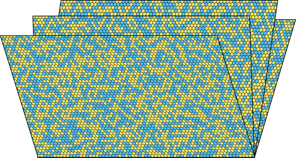
Consider the -pages book obtained by gluing copies of an upper-half plane along the bottom line , which is identified with , see Figures 1 and 3. We call these copies the pages of the book and identify with .
Our goal is to explore the behaviour of classical statistical physics systems on a -pages book. Of prime interest to us will be the family of Potts models as well as their corresponding graphical representations named Fortuin-Kasteleyn percolations.
1.1. Potts model on the book.
The Potts models are archetypical examples of statistical physics systems undergoing a phase transition in two dimensions. Fix an integer . For a finite graph of an infinite graph (we sometimes write if ), attribute a spin variable belonging to a certain set to each vertex . When , one speaks of the Ising model and use instead of for . A spin configuration is given by the collection of all the spins. Introduce the Hamiltonian of for free boundary conditions defined by
| (1) |
corresponding to a ferromagnetic nearest-neighbor interaction. For , we also define the Hamiltonian for monochromatic boundary conditions:
| (2) |
The above Hamiltonian corresponds to a ferromagnetic nearest-neighbor interaction. The Gibbs measure on at inverse temperature with (where is either free or monochromatic free) boundary conditions is defined by the formula
| (3) |
for every .
When or , one may define the Gibbs measure on at inverse-temperature with boundary conditions by taking the limit as of the previous measures. In infinite volume, the model undergoes a phase transition on and at some common [8] in the following sense. If
| (4) |
is the spontaneous magnetization of the model, then is equal to 0 if and is strictly positive if .
When , whether the phase transition is continuous (i.e. ) or discontinuous (i.e. ) has been the object of much interest in the past fifty years. It was proved in [33, 41] that the phase transition of the Ising model is continuous on . More generally, it was predicted by Baxter [5] that the phase transition of the Potts model on is continuous for and discontinuous for . See [14, 22] for a proof of this statement (see also [34] for a short proof in the case ).
In this paper, we investigate the question on and prove the following result.
Theorem 1.
There exists , such that for every , the -Potts model undergoes a first-order phase transition on . Equivalently, for every and every ,
As we shall explain below, it is natural in several respects to allow ourselves to strengthen the coupling constants along the edges of the gluing line .
For and , we then introduce the modified measure where is replaced by the Hamiltonian
(corresponding to changing coupling constants along the line from 1 to ) and the associated quantities , and .
To motivate the introduction of the parameter , let us briefly mention the slightly related problem of long-range Potts model on . The previous procedure is the analog of strengthening the coupling-constants between adjacent vertices in this context: As an example, in [2], coupling-constants are defined as and the following critical point is introduced ([2, 24], see also our recent work [15]),
In our present context, motivated by the predictions from [11, 23, 38, 39] (see Subsection 1.3 below), and by analogy with , we define below a notion of “optimal” number of pages needed to create a first-order phase transition. The advantage of the notions and comes from the fact that they are universal: they do not depend on the particular way of gluing pages together (as far as the glue is finite-range, say) or even the underlying lattice (it could be triangular or hexagonal for instance). For any , define
| (5) |
We obtain the following result on the behavior of the optimal number of pages depending on .
Theorem 2.
We have the following:
- (i)
- (ii)
- (iii)
for all .
We will discuss each of these items below, after Theorem 7 which is the analogous statement for FK percolation with cluster-weight .
Remark 1.
Interestingly, in the case , the effect of this first-order phase transition is to make the Ising model on each of the -pages independent of each other in the scaling limit. The statement below (written for , but it would also be valid for large enough and ) makes this factorization property more precise. Below, for a set , write .
Theorem 3.
Fix . Let be large enough so that . For any three sets , , and , containing a total of vertices that are all at a distance at least of , we have the following factorization property of -point correlations across :
If boundary conditions are prescribed instead, the condition on the parity of can be dropped and we get
Let us mention that the error term can be improved by looking more closely at our proof, but this is irrelevant for the conclusion of the paper.
1.2. Fortuin-Kasteleyn percolation on the book.
We now define the Fortuin-Kasteleyn percolation [25, 26] (we also refer to [28] for a manuscript and [12] for recent results). Let be a subgraph of an infinite graph , let be a partition of the vertices . A percolation configuration is an element . If we say that the edge is open, otherwise it is closed. We often see as a subgraph of with vertex-set and edge-set given by the set of open edges in .
The FK percolation measure on G with edge-weights and cluster-weight is defined by the formula
with if at least one endpoint is not in , and if both are, and where is the graph obtained from by wiring all the vertices in belonging to the same element of the partition . Let (resp. ) be the wired (resp. free) boundary conditions corresponding to the partitions equal to (resp. only singletons).
Below, we will use the notation (in ) if there exists a path of open edges between a vertex in and a vertex in (using vertices in only). We also write instead of when the set is a singleton, and to denote the fact that there exists an infinite path starting from .
We construct the FK percolation and on with wired or free boundary conditions by taking the limit as of the measures and . We also define, for an infinite graph containing the origin,
It was also proved that there exists such that for every integer and , is equal to 0 if and is strictly positive if . Again, the question of whether the phase transition is continuous (i.e. ) or discontinuous (i.e. ) was answered in the special case of : when , it is continuous [22] and when , it is discontinuous [14]. Here, we investigate this question on with . Our first result is as follows.
Theorem 4.
For any , there exists such that FK percolation undergoes a first-order phase transition on . I.e. for any ,
By choosing sufficiently large, the result also holds for arbitrary small and for free boundary conditions, i.e. for any ,
Proof of Theorem 1.
As in the case of Potts models, we define for any ,
The following result gives a precise picture of the optimal number of pages depending on . (See Fig. 2 for a plot of ). This extends Theorem 2 which was stated for Potts models ().
Theorem 5.
We have that
- a)
,
- b)
there exists such that for every ,
- c)
,
- d)
for all ,
- e)
for all .
We now comment on the different items in the above result.
- a)
- b)
- c)
The case is, arguably, the most interesting of all. As opposed to the case, this result will not be a straightforward consequence of (the proof of) Theorem 4. Its proof will be organized as follows:
- 1)
The proof that will be the focus of Section 5. The argument will be based on the random currents representation of the Ising model ([1, 13]). Random currents will indeed enable us to show that in the graph , far from the middle line , the spin system behaves (nearly) as if all edges along were wired together. This will be a key step of the proof as the precise values of arm-exponents in depend on what are the boundary conditions induced along .
- 2)
The second part of the proof is to show that pages are not sufficient to create an infinite cluster even if the edge-weights are arbitrary large on . Here, the second moment argument used for the case is not sufficient and a detailed analysis of the effect of a defect-line for critical Ising model is needed. This will be the subject of the companion paper [16].
- 1)
- d)
The proof that for any will consist in showing that a defect line with high coupling constants is sufficient in to create on its own an infinite cluster. The proof is given in Section 4. It will rely on the multiscale/renormalization argument built for Theorem 4 but will be simpler due to the planarity of .
- e)
Remark 2.
When (resp. ), it is not difficult to extend the analysis carried in this paper to a Book with pages (resp pages) in the following sense: consider the finite book with 3 pages (resp. 2 pages) of normal size and a fourth (resp third) page of size . These pages are glued along . We claim that by a slight adaptation of the multiscale proof in this paper, we can show that if the coupling constant is chosen high enough along , then with probability as , there is a macroscopic cluster in the book (resp long-range order in the book) with intensity larger than along the gluing line . This is consistent with predictions from [38, 39] (though with a different notion of pages).
In the whole paper, we focus on and . We drop them from the notation. In particular we write instead of . It will happen that we write , but we warn the reader that this means that the parameter is equal to (as the is always set to ).
1.3. Motivations from replicas and quantum spin systems.
Our results are motivated by several works in theoretical physics. To our knowledge, the first works which have considered the present gluing problem are the works [11, 23] by Cardy and Iglói-Turban-Berche. These two works rely on a renormalization group analysis in order to study the large tends to infinity case. Based on this RG analysis, both [11] and [23] suggest that if one glues an Ising model at on pages along a line, then the spins may spontaneously order near that line. The gluing of several pages of Ising arises naturally in their works in forms of replicas for a model with disorder, namely a Ising model with quenched magnetic disorder along its boundary .
More recently, in the works [38, 39] by Stéphan-Misguich-Pasquier and Stéphan, the authors combine conformal field theory arguments with numerical computations in order to give strong further support to these predictions. See also the simulations in [27].
The goal behind [38, 39] is in some sense also driven by the replica-trick but for a different underlying motivation than in [11, 23]. In these papers, the authors are interested in the Shannon entropy of the groundstate of the quantum Ising chain (or quantum Ising chain in transverse field), which is given on by the following Hamiltonian
For this Ising chain, the most natural basis, denoted , of is given by the eigenstates of which correspond to the actual spins in the classical two-dimensional model. In this basis, and for the critical parameter in the quantum Hamiltonian , the ground state can be written as
where denotes the probability for a classical Ising model11 1 For this correspondance to hold, the classical Ising model should not be on a -grid but rather on a lattice. We will not enter into these considerations here, but simply mention that our study does extend to this more general framework using a similar renormalization framework and the statement of [18] guaranteeing that the behaviour on is similar as the one on . in the infinite cylinder to generate at the configuration at the middle slice of the cylinder . The Shannon Entropy of the Quantum Ising chain in the basis is then defined as
The connection with Book-Ising goes as follows: one can express the entropy as a limit as of the so-called Renyi’s entropies :
Now, in the spirit of the celebrated Parisi replica’s trick, the idea in [38, 39] is to analyze via the analysis of the Renyi entropies . The link with Book-Ising is that the measure on which assigns a weight on each configuration proportional to can be realized as a Book-Ising on pages (where pages here are semi-infinite cylinders ). See Fig. 3 (with squares instead of semi-infinite cylinders).
Organization of the paper.
Acknowledgements.
The second author wishes to thank Jean-Marie Stéphan for very inspiring discussions on the physics side of this problem. The first author is funded by the ERC CriBLaM, the Swiss FNS and the NCCR SwissMap. The research of the second author is supported by the ERC grant LiKo 676999. The third author was funded by the ERC grant 851565.
2. Preliminaries and disconnection exponent on the Book
2.1. Disconnection exponent.
In the rest of the paper, depending on the context, will be either the box of size in . We will extensively rely through this paper on the following event. For any , let be the event that there exists a page in which is disconnected from in by a path in . Let us mention that the complementary event can also be interpreted using the dual representation of the Fortuin-Kasteleyn percolation on the page, where is defined as follows. For each page , let be the dual graph of , and set , where is the unique dual edge that crossed in its center. Then, we speak of a dual-open path of dual-edges for a path in which is open in (we write for the existence of a dual connection between the sets and ). Then, corresponds to the event that in each page, there exists a dual-open path from to , see Fig. 4.
Below, we will speak of a critical exponent for a family of probabilities as follows
Morally speaking, this critical exponent is ruling the speed of algebraic decay – in – of the probabilities . In what follows, we expect the families of probabilities (but this is currently unknown for most of the families under consideration) exhibit a behaviour of the form
where is a quantity that tends to 0 as tends to 0, but this is currently unknown for a number of them.
Definition 6.
The disconnection exponent is defined as the critical exponent of the family .
This disconnection exponent will be of central importance in this work as its value will exactly detect when (as increases) the phase-transition becomes first-order instead of second-order. Indeed the main ingredient for the proof of our main results.
Proposition 7.
For every , if is such that , then there exists such that
In other words, implies .
2.2. Arm-exponents in .
The following three one-arm exponents in the upper-half plane will help us obtain estimates on the disconnection exponent uniformly in . As they are not known to exist, we define them like the disconnection exponent (in the notation below we ignore the parameter as it is set to ):
- •
: the critical exponent for the family
- •
: the critical exponent for the family
- •
: the critical exponent for the family
Note that with these definitions, the following special cases are known:
- i)
- ii)
(see e.g. [17]).
For future reference (we will use these estimates later on), we write instead of .
Remark 3.
Since the free (resp. wired) boundary conditions are helping (resp. disadvantaging) a dual connection, we have that . We will note use this fact, but for all , one has
2.3. Proof of Theorem 4 given Proposition 7.
We first prove the following uniform control on .
Proposition 8.
There exists such that for every , .
Proof.
Assuming Proposition 7 holds, it is enough to find an integer large enough so that for every .
The most trivial bound on is obtained as follows. For not to occur, it must be that in each page, is connected to in the dual configuration ; see Fig. 4. Using the comparison between boundary conditions, one may split the book into disconnected pages and use that this event has a probability smaller than in each page. This reasoning gives
It is known from [32, 37] that , so we already obtain at this stage a proof of the upper-bound in item a) of Theorem 5, i.e
For the remaining , it was proved in [22] that , thus giving the existence of such that . The problem with this bound is that it deteriorates when tends to 4, for which is expected to be equal to 0. This reasoning would force us to choose a number of pages tending to as .
A slightly better bound is obtained by observing that by successively conditioning in each page, for all but the last page, the probability of having a dual path connecting is connected to in a page is smaller than since there exist at least two undiscovered pages (and therefore by comparison between boundary conditions the occurrence of the connection is smaller than the one under the full plane measure), which explains why we introduced above the exponent . (This observation will also be used in the proof of Lemma 12). This domination is valid as long as there are at least two remaining pages so we get
This exponent is know from [22] to be larger than some constant uniformly on . As a consequence, we deduce that uniformly in which thus proves the content of Proposition 8.
Remark 4.
As we will obtain by other means when (in Section 4), we may have focused here only on the case which is slightly simpler since the bound would already be sufficient. Yet we decided to include the proof below which works uniformly in because it highlights well the different boundary conditions at work near the joint line and because the exponent will also play a key role later (in the proof of the anchoring Lemma 12).
Remark 5.
In fact, we expect that as soon as percolation occurs in , then
This comes from the intuition that the infinite cluster at in is staying close to the axis, and that this cluster acts as a wiring of vertices. We will turn this intuition into a proof thanks to the random currents representation in the special case of in Section 5. As should be equal to (see [36, 20]), this is consistent with our results (and predictions) on in Theorem 5.
Proof of Theorem 4 given Proposition 8.
To prove Theorem 4, it remains to treat the general case where the edge-density on is an arbitrary number . (The same argument also applies to the case where edges along have the same weight as the other edges). Consider such that and such that the process given by the pairs of neighboring edges and in that are connected to each other in is dominating a FK percolation of parameter on (the existence of this integer is easy using finite energy). Then, one can easily check that the restriction to of FK percolation with parameter on is dominating FK percolation on with parameters and . This concludes the proof.
3. Proof of Proposition 7
3.1. Preliminaries.
Let . We call a cluster in a connected component of the graph with vertex-set and open edges with both endpoints in . We will use the notion of -block to be the translate by the vector of the union, in each page, of the squares . For simplicity we write instead of . Given a block , we write for the cluster in which has the largest intersection with (when there is more than one, pick one according to a deterministic rule).
We will need the following two definitions.
Definition 9 (-bad block).
A -block is -good if . When a block is not -good, we call it -bad. Introduce
Definition 10 (bridged block).
A -block is bridged in if there exist and such that
- •
and are -good.
- •
and are connected together in .
Introduce
3.2. Bound on .
The core of the proof of our theorem will be the following proposition.
Proposition 11.
For every and , there exists such that
| (6) |
for every , , , and .
The proof of Proposition 11 is divided into two independent lemmata, referred to as the anchoring lemma and the bridging lemma.
For , introduce the set to be the union of the half-annulus and the blocks with . For a set , introduce the boundary condition to be the wired boundary condition on , and free elsewhere (see Fig. 5).

Lemma 12 (Anchoring Lemma).
There exists such that for every , every integers , every , and every path from to staying above ,
Proof.
Consider the increasing coupling between random-cluster models (see e.g. [28] for details) between two configurations with
where is the restriction of to the first two pages (it is a subset of the plane), defined as follows (see for example [21]). The coupled configuration is written as an increasing function of i.i.d. uniform variables in which are indexed by the edges of . To define
we proceed inductively: the variables are used one at a time to sample given the values of the former edges that have been fixed . Once all edges have been fixed, the remaining variables are used to sample the remaining edges for .
Define now to be the number of pairs with and such that
- •
is -good in ;
- •
;
- •
is connected to in .
The fact that is increasing implies FKG property for , which itself gives
On the one hand, standard crossing estimates and mixing properties of the critical FK percolation with give that there exists such that
On the other hand, the definition of -good -blocks immediately gives that
Altogether, we deduce the following lower bound on the first moment of :
We now turn to a bound on the second moment. By dropping the first condition, replacing the second by , and observing that each belongs to at most 2 blocks, we obtain that
A standard application of crossing probabilities and quasi-multiplicativity, see e.g. [??], shows that
Cauchy-Schwarz inequality implies that the probability that is bounded from below by . Since implies the event under consideration, the claim is proved.
Remark 6.
At first sight, a natural way to try proving the Anchoring Lemma would be to run a direct second moment argument on the number, say , of points on the middle line which are connected to in the first page instead of considering the more complicated . This works well in the case, but as soon as this strategy seems difficult to implement. Indeed, the first moment would involve in this case the one-arm event in a page but for the FK measure in the full book graph . So far so good, but difficulties arise when controlling as a quasi-multiplicativity statement for this arm event would be needed. One way to achieve this would be to prove a version of the mixing lemma (as in [17] in the plane) for the FK measure on the book . This does not seem straightforward as different pages may interact via the joint line . This is the reason why we introduce in the proof above a suitable coupling argument in order to transfer the problem to a setting where one can apply a more standard second moment method.
We now turn to the Bridging lemma. For integers and a small real number , set and let be the event that there are at least integers such that and occurs.
Lemma 13 (Bridging Lemma).
For every , there exist and an integer such that for every and large enough,
Proof.
By monotonicity, it suffices to show the result for . Fix . By definition of , there exists such that for every large enough and ,
| (7) |
By conditioning on the configuration outside , the spatial Markov property and the comparison between boundary conditions combined with the previous displayed equation implies that the probability that occurs is larger than . In particular, the number of integers with such that occurs is dominating a binomial random variable with parameters and . We deduce that for small enough, the probability that there are fewer than such is smaller than .
We are now ready to dive into the proof of Proposition 11.
Proof of Proposition 11.
Fix and observe that if there is nothing to do22 2 At this stage one may wonder why we put in the right-hand side of (6) instead of simply . The reason comes from the conjecture that (7) can be obtained essentially in terms of the probability of a dual connection with wired boundary conditions on , and that in order to do that, one may want to assume that . We refer to Sections 4 and 5 for details of such an application.. We therefore now assume the opposite. Since the box of size around is included in and being bridged is an increasing event, the comparison between boundary conditions implies that it suffices to treat the case in the block with .
Fix and consider and given by the Bridging Lemma. Also, write . Thanks to the Bridging lemma and the comparison between boundary conditions,
and it suffices to show that there exists a universal constant such that

We now introduce a few quantities (see Fig. 6). For , let be the inner-most path in disconnecting and in (note that it is a subset of ). Define to be the set of in that are surrounding by , with the convention that the set is when does not exist. Similarly, define and as the corresponding quantities in . Finally, consider the set
as well as the set of pairs for which exists, and the set of triplets with and .
Now, condition on the states of the edges in and let be the boundary conditions that they induce on . Note that it can be done without revealing any edge outside of and that is measurable in terms of the states of these edges. For each , say that ends in and on the left and right respectively. For , let be the event that there exists with such that is -good and is connected to in . Similarly, define on the left. The comparison between boundary conditions and the anchoring lemma imply that
where in the last line we used the fact that on , , and that the assumptions that and guarantee the existence of .
3.3. Proof of Proposition 7.
The proof of Proposition 7 relies on the idea that clusters at scale and local density will merge and with high probability create new clusters at scale of local density slightly smaller than (this slight loss of density allows us to lose a few clusters at scale in the process). More precisely, we prove the following renormalization inequality.
Lemma 14.
Let such that and . There exist large enough (depending on and ) such that the following holds. For every and for every integers and ,
| (8) |
Proof.
Fix . Let be a large constant to be chosen later and set . For , let be the event that is -bad and all the blocks are -good for , and set
| (9) |
Observe that if all -blocks , , are -good, then the assumption that imposes that all the clusters are connected together in , which implies the existence of a cluster in with cardinality larger than . In particular, if is -bad, then either there exist two disjoint -bad -blocks, or there exists such that occurs. The union bound implies
| (10) |
By the spatial Markov property and the comparison between boundary conditions, we have
| (11) |
It remains to bound the first term in (10), which is the object of the end of the proof. If all -blocks with are -good, the same argument as above implies that is -good, therefore whenever . Now, let . Note that if is bridged in , then is also -good. Furthermore, when is not bridged (this event does not depend on edges in ), for to occur then must be -bad. As a consequence, the spatial Markov property and the comparison between boundary conditions implies that
| (12) |
where in the last line we invoked Proposition 11 for . Select so large that
Proof of Proposition 7.
Let satisfying . Choose and (where is provided by Lemma 14) such that the sequences
satisfy for every . Now, set so large that
and consider the sequence of scales defined33 3 Note that it gives for all . by
| (13) |
Applying Lemma 14 to , we see that the sequence satisfies
By induction, we obtain that for every , and therefore,
First using the estimate above and then translation invariance, we get that for every ,
| (14) |
Dividing both sides by , we obtain
which by measurability implies that the probability that 0 is connected to infinity is larger than or equal to .
4. Proof of Theorem 5 for
In this section, we prove the following two claims of Theorem 5: first we show that , when and second, we prove that for all and that . The more subtle case of will be analyzed in the next section with the help of random currents.
We start with the following proposition corresponding to the first claim.
Proposition 15.
For every , there exists such that for every and ,
In particular, .
The proof is based on a second-moment argument.
Proof.
Define the number of edges such that the endpoints of are respectively dual connected to the top of in the upper half-plane, and to the bottom of in the lower half-plane. Under (for which is completely wired), both pages behave independently and we immediately get that
In the other direction, the second moment gives, using classical quasi-multiplicativity estimates
where in the last inequality we used a result from [20] stating the existence of such that for every ,
| (15) |
Overall, we get by comparison between boundary conditions and Cauchy-Schwarz that
Now, on (which does not prescribe anything on edges in ), is not crossed horizontally if any of the edges of such that the endpoints of are dual-connected to top and bottom is in fact closed. Since there is at least one such edge, we get that
This concludes the proof of the first part of the proposition. For the second part, ergodicity gives that since otherwise the crossing probability would tend to 1.
We now turn to the other claim, which we split in two.
Proposition 16.
For any , we have .
Proof.
We wish to prove that for large enough, . In order to do that, we only need to prove the equivalent of Proposition 11, i.e. that for some constant , there exists such that
| (16) |
for every , , , and .
To do that, observe that for not to be bridged in ,
- •
either there must be a -bad box , an event which occurs with probability smaller than ,
- •
or all the boxes are -good, in which case if is the cluster gathering all the , we have that is dual connected to above and below .
Yet, when working on , one notices that contains a crossing from left to right in . In particular, conditioned on the bottom-most such crossing and everything below it, the spatial Markov property together with the comparison between boundary conditions of the model imply that the probability that there exists a dual path from to above is bounded by the probability that there exists a dual-connected path in from to , with free boundary conditions on and wired on the bottom. In particular, it is bounded by using classical mixing properties coming from [22]. Now, it was proved in [20] that for every (it was not done for but the same proof extends), there exists such that for every ,
| (17) |
Altogether, we deduce that for some constant ,
Similarly, one proves that
Combining this two displayed inequalities with the two bullets above gives (16) for , a fact which concludes the proof.
Proposition 17.
For any , we have .
Proof.
The lower bound is a straightforward consequence of the strong RSW Theorem from [22], that implies that on , the probability that there exists a dual path from to surrounding in is bounded from below by a constant . This contradicts the fact that this probability should tend to 0 for to be connected to infinity.
5. Book-Ising with three pages and random currents
The purpose of this section is to show that a first-order phase transition already arises with only pages for Book-Ising (). This corresponds to and our proof is consistent with the prediction from [38, 39]. The main technique will involve random currents. To highlight the main ideas, before handling the graph , we will start in the subsection below with an interesting question on its own where a positive (i.i.d) density of sites along the middle line are oriented in the direction. We will only give a short sketch of proof for the toy-model and will leave the detailed proof to the true Book-Ising (as such the former may be viewed as an outline of proof of the second in a simpler setting).
5.1. A positive density of is indistinguishable from a boundary condition.
In this subsection, we will give a sketch of proof of the following result: the decoupling property from Theorem 3 holds in the simpler setting of the half-plane where a positive density of sites on are wired together. This will serve as a useful toy model for Theorem 3. The reader comfortable with the random current terminology may skip this section if needed. The statement above is a 2D version of a result by Bodineau [10].
Let us set some notations: will denote the bias of our Bernoulli quenched disorder along the line . Let be i.i.d. Bernoulli random variables attached to each site on the middle line . Given , will denote the (random) graph where all points for which are wired together. Finally, denotes the Ising measures on with boundary conditions.
Theorem 18.
For any and any , there exist so that for any set made of vertices at a distance at least of , then with probability at least in the quenched disorder , we have
Remark 7.
Note that by Griffiths inequalities, we deduce that if we consider the graph constructed like but from instead of , we immediately get that for every three sets , and made of vertices all at a distance at least from , we have that with probability at least in the quenched disorder , we have that
The proof of the theorem requires the introduction of another representation, called the random-current representation. We refer to [1, 13] for details on this representation and briefly define it here. A current on is a function from to . A source of is a vertex for which is odd. The set of sources of is denoted by . Also set
Currents are useful as they lead to the following expression for spin-spin correlations:
| (18) |
For more general spin-observable , , one has the expression
Also, a classical use of the switching lemma enables one to compare the spin-spin correlations on two graphs as follows:
| (19) |
where attributes a weight proportional to if and otherwise, and the sign means that we take the product measure (see for example [3, Lemma 2.2]). For a general spin-observable , with , the identity becomes
where is the event that any cluster of intersecting must intersect at an even number of points.
We shall also need these expressions in the case of a graph with boundary conditions. This means that some points (called the boundary of ) are connected to an extra vertex called the ghost vertex. (See [13] for a detailed exposition). In such a case, the last expression for example reads as follows:
where currents under and are now allowed to go through the ghost vertex and their boundary is only considered on all vertices but the ghost (also is now the event that all the clusters which intersect are either connected to the ghost or intersect at an even number of points).
Sketch of proof of Theorem 18.
We will show that there exists such that for every made of vertices at a distance at least from ,
For any large , let be the finite random graph obtained from by connecting all the vertices which are such that to the ghost. We have
Applying the above formula, it remains to bound from below (for any large ) the following average with respect to :

We proceed as follows:
- (1)
Sample according to . If restricted to is already in , then whatever and are, we must have .
- (2)
Suppose then that this is not the case. Then, there is at least one cluster of intersecting and reaching (and there are of course at most such clusters). By union bound, let us focus on the case of only one point, say , and let us assume that connects with . Among all points in which are connected to via , choose to be, say, the furthest on the left and to lighten the notation assume it is equal to the origin. Notice that is measurable with respect to and that neither nor have been sampled yet.
- (3)
Let then sample so that the subgraph is now well defined.
- (4)
- (5)
Assuming is sufficiently dense around , the rest of the proof consists in showing that with probability at least , the current will create a bridge from to which, by planarity, will necessarily intersect . As such will be connected to the ghost via as desired.
- (6)
We also discuss a slightly more difficult theorem, but which is closer to the one in the next section. Let be the FK percolation measure where all the sites are wired together.
Theorem 19.
For any and any , there exist so that with probability at least in the quenched disorder , we have
| (20) |
Steck of proof of Theorem 18.
Define the subsets of :
Let be the finite graph in which all vertices in are connected (wired) to a ghost vertex and all vertices in are connected (wired) to a different ghost vertex and where the rest of of the boundary is free. Let also be the graph where all vertices in are connected to while all vertices in are connected to and where the rest of the boundary is free. The monotony properties of FK percolation and the Edwards-Sokal coupling give that
Notice that we have . Similarly as in the above proof, we may now use the switching lemma via the above identity (19) to obtain
From now on, the proof can be concluded in two steps.
- (1)
It can be extracted for instance from [17] that
- (2)
The second step is very similar to the argument outlined above: under , will connect at least a point to a point . The goal is thus to show that will create with high probability a bridge which will connect and to . To prove this, we argue as above: we set an intermediate scale and we claim that with probability at least , the sets (resp ) will be sufficiently dense at scale to create many bridges thanks a coupling between sourceless random-current and FK percolation with parameter (see the proof of Lemma (21) for a detailed proof).
At this stage, there is a subtle but important difference compared to the argument in the previous sketch of proof. It could be that the points and could be close to or . In such case, one cannot really use the argument described above. Yet, it can be proved in this case that the probability that itself is connected to a vertex of close (say at a distance at most ) to or is bounded by (see the next section for details).
5.2. Proof of Theorem 2(i)
The core of the proof will be the following result.
Proposition 20.
There exist such that for every and such that divides , every , every , and every ,
We start by explaining how to adapt the proof of Theorem 4 using Proposition 20 to obtain Theorem 2(i).
Proof of Theorem 2(i).
Fix and and assume for a moment that is chosen so that . When applied to , we see that the previous proposition implies that
From this, one can easily adapt the proof to reach the conclusion of the bridging lemma with (note that except for the first and last values of , the right-hand side is bounded by ). After this, Proposition 11 follows in the same way. Also, note that the assumption that is harmless as otherwise the statement of Proposition 11 is obvious. Once Proposition 11 has been obtained, the rest of the proof of the theorem is the same as for Theorem 4.
We conclude our paper by the proof of Proposition 20.
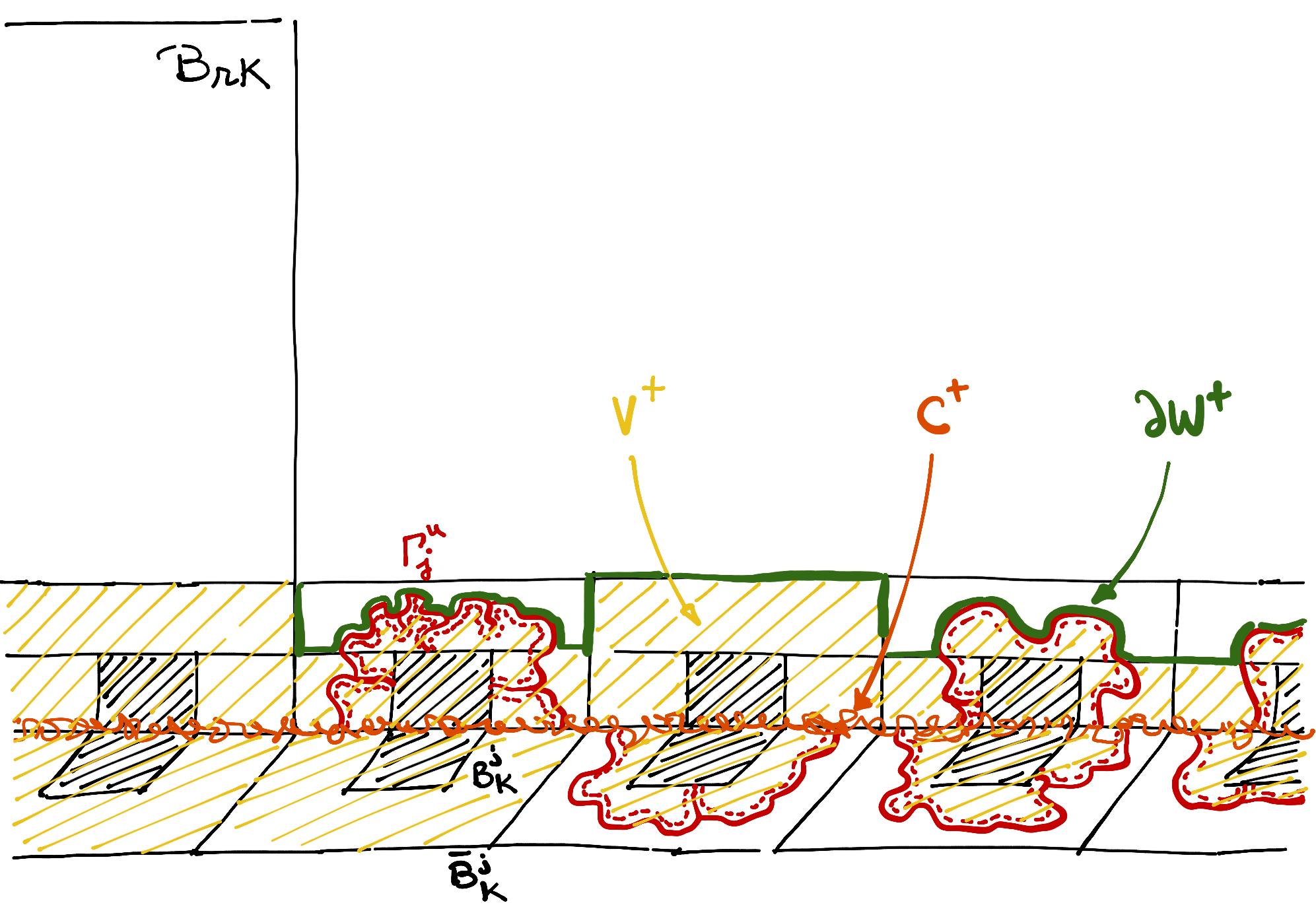
Proof of Proposition 20.
Set . We may assume as otherwise the statement is obvious. Let be the event that all the -blocks are -good for . By definition of ,
| (21) |
Below, we recommend to take a look at Fig. 8. Introduce to be the set of vertices at a distance at most from . Define to be the sets of indexes divisible by 6, positive or negative depending on whether is or , for which is surrounded in by a circuit in connecting to . Call the inner-most such circuit . Let
Adapting the anchoring lemma and using that , we deduce that for some small enough,
Using the comparison between boundary conditions, we may compare to independent random variables to get that dominates a binomial random variable with parameters and , so that for some constant small enough and independent of everything else,
| (22) |
We deduce from (21) and (22) that it suffices to show that
| (23) |
We now focus on deriving this inequality.
On , call the union of the for , which since is made of one single cluster. From now on, let be the (random) subset of obtained as
- •
the union of all the for ;
- •
the vertices of surrounded by the for every divisible by 6 for which the path exists for every ;
- •
the union of the for the remaining which are divisible by 6.
Similarly, one defines and with instead of . Also, set be the set of edges with both endpoints in .
Condition on for some configuration belonging to (by this we mean that any configuration coinciding with on is in ). Let be the graph induced by the edges in and be the boundary condition on obtained from the configuration equal to on , and 0 on the remaining part of .
The comparison between boundary conditions implies that for every ,
It therefore suffices to prove that each term on the right is smaller than . From now on, we call a pair , with a subset of and a boundary condition on possible if there exists and such that and . In this case we write for the corresponding set (they can be read off from and in a unique fashion).
Let be the intersection of with . Consider the boundary condition obtained from by wiring all the vertices in together, and all those in together. For every possible , going to the complement implies that
The following lemma will therefore conclude the proof.
Lemma 21.
There exist independent of everything such that for every possible ,
As in the case of Theorems 18 and 19 for which we sketched the proofs earlier, the derivation of this lemma will rely on the random-current representation. A first key property will be the identity (19) which follows from the switching lemma.
We will use also a second property of our model, which is a coupling between sourceless random-current and FK percolation with parameter . More precisely, consider the coupling obtained by considering and obtained from by setting
where is an independent family of Bernoulli random variables of parameter . Then, one has that under , with . While the recipe to get from is obvious, let us mention that in the other direction, for , one may recover the edges on which is odd by taking a uniform even subgraph of (see [4, 29, 31]).
We are now in a position to prove the lemma.
Proof.
Consider the graphs obtained from by identifying all the vertices in into two vertices , and obtained from by identifying vertices in to . Note that can be seen as a subgraph of where the latter is obtained from the former by adding edges with infinite coupling constants (or equivalently infinitely many edges with standard coupling constant) between the vertices of and ).
We have that
so that (19) gives that
and it therefore suffices to bound the probability on the right-hand side.
First, observe that the coupling between random-current and FK percolation implies that
Similarly for , , and . We therefore may restrict to realizations of that necessarily contain a path of from to , going say from to , with
As a consequence, it suffices to prove that in , with large probability there exists a path of from vertices in respectively on the left and right of (call the two parts and ). The same estimate will also holds for .
In order to do that, we write instead of and use the increasing coupling between and the random-cluster model described before the proof. It is sufficient to prove that
| (24) |
Indeed, on this event, one may divide clusters in pairs, and observe that each pair of clusters contains a loop (with one path in one cluster and the other in the other one) of connecting to with probability at least thanks to the fact that the odd part of is obtained from by taking an even subgraph of uniformly at random. Therefore, the probability that there exists no path at all will be smaller than .
To prove (24), first shift the whole configuration by in order to recenter everything around 0. On the one hand, crossing estimates imply that for such that ,
| (25) |
for some constant independent of everything. On the other hand, if denotes the intersection of with the annulus , we want to prove that
| (26) |
This will conclude the proof by observing that (25) and (26) together with the spatial Markov property and the comparison between boundary conditions easily imply (24) by following a proof quite similar to the bridging lemma.
To prove (26), we use a second-moment method very similar to the proof of the anchoring lemma. Let be the number of pairs and with connected to (recall the definition of these paths from the previous section, and remember that the whole configuration has been shifted by ). Note that by definition of a possible pair (since belonged to ), there are of order pairs of . Also, an easy comparison between boundary conditions and use of crossing estimates implies that
In the other direction, the comparison between boundary conditions and a standard use of the quasi-mulitiplicativity property gives that
5.3. Proof of Theorem 3.
The proof of the decoupling between the pages of stated in Theorem 3 follows easily by combining the proof of Proposition 20 together with the (sketch) of proof of the decoupling property from Theorem 18. Let us shortly explain why we have an error term in Theorem 3 versus in Theorem 18. To prove Theorem 3, we rely on the multiscale framework used throughout the paper. In particular, if all points in are at a distance at least from , consider such that
Recall (footnote below (13)) that . This implies in particular that , when is large enough. Let us now proceed as in the proof of Theorem 18 and let be the furthest point on the left of the joint line of an cluster emanating from, say the first point (other possible points being connected to via are handled similarly by union bound). We now consider the blocks at scales around the point . From our inductive proof, we know that each of these -block is good with probability at least . (See the estimates on below (13)). This implies that with probability at least , all -blocks around the point and up to distance are good. We can now use this overlapping chain of good blocks as in the proof of Lemma 21 to produce a bridging with the random current with probability at least which is the same as and thus concludes our proof.
References
- [1] M. Aizenman. Geometric analysis of fields and Ising models. I, II. Comm. Math. Phys., 86(1):1–48, 1982.
- [2] M. Aizenman, J.T. Chayes, L. Chayes, and C.M. Newman. Discontinuity of the magnetization in one-dimensional ising and potts models. Journal of Statistical Physics, 50(1-2):1–40, 1988.
- [3] M. Aizenman, H. Duminil-Copin, V. Sidoravicius. Random currents and continuity of Ising model’s spontaneous magnetization. Communications in Mathematical Physics, 334(2):719–742, 2015.
- [4] M. Aizenman, H. Duminil-Copin, V. Tassion, S. Warzel. Emergent planarity in two-dimensional Ising models with finite-range interactions Inventiones mathematicae, 216(3):661–743, 2019.
- [5] R.J. Baxter. Potts model at the critical temperature. Journal of Physics C: Solid State Physics, 6(23):L445, 1973.
- [6] V. Beffara and H. Duminil-Copin. Smirnov’s fermionic observable away from criticality. Ann. Probab., 40(6):2667–2689, 2012.
- [7] V. Beffara and H. Duminil-Copin. Lectures on planar percolation with a glimpse of Schramm Loewner Evolution. Probability Surveys, 10:1–50, 2013.
- [8] V. Beffara and H. Duminil-Copin. The self-dual point of the two-dimensional random-cluster model is critical for . Probab. Theory Related Fields, 153(3-4):511–542, 2012.
- [9] I. Benjamini, G. Kalai and O. Schramm. Noise sensitivity of Boolean functions and applications to percolation. Publications Mathématiques de l’Institut des Hautes Études Scientifiques, 90(1):5–43, 1999.
- [10] T. Bodineau, Translation invariant Gibbs states for the Ising model. Probability theory and related fields, 135(2):153–168, 2006.
- [11] J.L. Cardy, The Ising model in a random boundary field. Journal of Physics A: Mathematical and General, 24(22):L131, 1991.
- [12] H. Duminil-Copin. Lectures on the Ising and Potts models on the hypercubic lattice, arXiv:1707.00520, 2017.
- [13] H. Duminil-Copin. Random currents expansion of the Ising model. arXiv:1607:06933, 2016.
- [14] H. Duminil-Copin, M. Gagnebin, M. Harel, I. Manolescu, and V. Tassion. Discontinuity of the phase transition for the planar random-cluster and Potts models with . arXiv:1611.09877, 2016.
- [15] H. Duminil-Copin, C. Garban, and V. Tassion. Long-range models in revisited. Preprint, 2020.
- [16] H. Duminil-Copin, C. Garban, and V. Tassion. Defect lines for Potts model and FK percolation. In preparation, 2020.
- [17] H. Duminil-Copin, C. Hongler, P. Nolin. Connection probabilities and RSW type bounds for the two-dimensional FK Ising model. Communications on pure and applied mathematics, 64(9), 1165-1198, 2011.
- [18] H. Duminil-Copin, J.-H. Li, I. Manolescu. Universality for the random-cluster model on isoradial graphs. Electronic Journal of Probability, 23, 2018.
- [19] H. Duminil-Copin, I. Manolescu. Planar random-cluster model: scaling relations. In preparation, 2020.
- [20] H. Duminil-Copin, I. Manolescu, and V. Tassion. Planar random-cluster model: fractal properties of the critical phase. arXiv:2007.14707, 2020.
- [21] H. Duminil-Copin, A. Raoufi, and V. Tassion. Sharp phase transition for the random-cluster and potts models via decision trees. Annals of Mathematics, 189(1):75–99, 2019.
- [22] H. Duminil-Copin, V. Sidoravicius, and V. Tassion. Continuity of the phase transition for planar random-cluster and Potts models with . Communications in Mathematical Physics, 349(1):47–107, 2017.
- [23] F. Iglói, L. Turban and B. Berche. Critical behaviour near multiple junctions and dirty surfaces in the two-dimensional Ising model. Journal of Physics A: Mathematical and General 24.17:L1031, 1991.
- [24] J.Z. Imbrie and C.M. Newman. An intermediate phase with slow decay of correlations in one dimensional percolation, ising and potts models. Communications in mathematical physics, 118(2):303–336, 1988.
- [25] C. M. Fortuin and P. W. Kasteleyn, On the random-cluster model. I. Introduction and relation to other models, Physica, 57:536–564, 1972.
- [26] C. M. Fortuin, On the Random-Cluster model, Doctoral thesis, University of Leiden, 1971.
- [27] P. Grassberger. Critical phenomena on k-booklets. Physical Review E, 95(1):010102, 2017.
- [28] G. Grimmett, The random-cluster model, Grundlehren der Mathematischen Wissenschaften [Fundamental Principles of Mathematical Sciences], vol. 333, Springer-Verlag, Berlin, 2006.
- [29] G. Grimmett and S. Janson, Random Even Subgraphs, Electron. J. Probab, 16(1), 2009.
- [30] H. Kesten, Scaling relations for D-percolation, Communications in Mathematical Physics, 109(1):109–156, 1987.
- [31] T. Lupu and W. Werner, A note on Ising random currents, Ising-FK, loop-soups and the Gaussian free field, Electron. Commun. Probab., 21(13), 7 pages, 2016.
- [32] Y. Ikhlef and A. Ponsaing, Finite-Size Left-Passage Probability in Percolation, J Stat Phys., 149:10–36, 2012.
- [33] L. Onsager, Crystal statistics. I. A two-dimensional model with an order-disorder transition, Phys. Rev. (2), 65:117–149, 1944.
- [34] G. Ray, Y. Spinka A short proof of the discontinuity of phase transition in the planar random-cluster model with , arXiv:1904.10557v1 (2019).
- [35] O. Schramm and S. Smirnov. On the scaling limits of planar percolation. With an appendix by C. Garban. The Annals of Probability, 39(5):1768–1814, 2011.
- [36] S. Smirnov. Conformal invariance in random cluster models. I. Holomorphic fermions in the Ising model. Ann. of Math. (2), 172(2):1435–1467, 2010.
- [37] S. Smirnov and W. Werner, Critical exponents for two-dimensional percolation, Math. Res. Lett., 8(5–6):729–744, 2001.
- [38] J.M. Stéphan, G. Misguich and V. Pasquier. Rényi entropy of a line in two-dimensional Ising models. Physical Review B, 82(12), 125455, 2010.
- [39] J.M. Stéphan. Shannon and Rényi mutual information in quantum critical spin chains. Physical Review B, 90(4), 045424, 2014.
- [40] W. Werner. Lectures on two-dimensional critical percolation. In Statistical mechanics, volume 16 of IAS/Park City Math. Ser., pages 297–360. Amer. Math. Soc., Providence, RI, 2009.
- [41] C.N. Yang, The spontaneous magnetization of a two-dimensional Ising model, Phys. Rev. (2), 85:808–816, 1952.