State distinguishability under weak measurement and post-selection: A unified system and device perspective

The initial preparation procedure generates spin-up states $\ket{\uparrow_\xi}=\cos\alpha/2\ket{\uparrow_x}+\sin\alpha/2\ket{\downarrow_x}$ (all density matrices are represented in the measured $\sigma_{z}$ basis)

For the intermediate projective measurement (without post-selection), which will destroy all coherence, the state is left in a statistical mixture of eigenstates $\ket{\uparrow_z}$ and $\ket{\downarrow_z}$

On the contrary the weak measurement only disturbs the initial state slightly, such that the exact system state is given by

Note that following the original derivation of the WV in aharonov1988result; aharonov1990properties, the decoherence factor $\exp[-g^{2}/(2\Delta^{2})]$ vanish and is identical with (III.1) when $g/\Delta\to 0$.

To quantify the disturbance of the system during the measurement sequence we use the trace distance between to density matrices $D(\rho_{1},\rho_{2})=\frac{1}{2}\Tr(\abs{\rho_1 - \rho_2})$ as a measure of how much the system state after the measurement deviates from the state prior to the interaction. The trace distance has the properties of a metric in the space of density matrices and a natural interpretation as the distinguishability between the two states fuchs1999cryptographic; nielsen2002quantum. For a spin-1/2 particle the trace distance between two states $\rho_{1}$ and $\rho_{2}$ with matrix elements $(\rho_{1/2})_{ij}$ has the simple form $D(\rho_{1},\rho_{2})=\sqrt{a^{2}+\absolutevalue{b}^{2}}$, where $a=(\rho_{1})_{11}-(\rho_{2})_{11}$ and $b=(\rho_{1})_{10}-(\rho_{1})_{10}$, are the differences in the population and coherence of the two density matrices, respectively.

At first, we consider the trace distance between the initial state $\rho_{i}$ and the intermediate state after a strong or weak measurement. For a strong von Neumann measurement we have $D(\rho_{i},\rho_{s})=\frac{1}{2}\absolutevalue{\cos\alpha}$, while for the weak measurement

demonstrating that the distinguishability between the state prior to the measurement and the state after the measurement is smaller for the weak measurement case than in the projective counterpart. Interpreting $D(\rho_{i},\rho_{s/w})$ as the amount the system state changes, or equivalently, the amount of disturbance caused by the measurement, confirm that a weak measurement is minimal disturbing. For $g/\Delta\to 0$, such that $D(\rho_{i},\rho_{w})=0$, the initial state is undisturbed, but no information is obtained. In the opposite limit $g/\Delta\to\infty$ we recover the effect of a projective measurement, leading to an enhanced information gain in the trade-off for a larger state disturbance fuchs2001information. Both measurements are non-disturbing for $\alpha\in\{\pi/2,\,3\pi/2\}$, which is the case for a procedure which initially prepares an eigenstate of the measured observable.

To quantify the difference between both experimental schemes in terms of the corresponding amount of preserved coherence (the populations remain unaltered), we show the difference of the trace distance of both schemes $\mathcal{D}(\alpha)=D(\rho_{i},\rho_{s})-D(\rho_{i},\rho_{w})$ for different values of the order parameter $g/\Delta$ in Fig. 2 (a). This is a direct measure of the preserved coherence in a weak measurement process and is associated with the conservation of information inside the system during a weak measurement. For larger $\mathcal{D}(\alpha)$, and thus smaller $D(\rho_{i},\rho_{w})$, the amount of preserved coherence increase and is maximal for $\alpha\in\{0,\,\pi\}$ when the initial state $\rho_{i}=(\ket{\uparrow_z}\pm\ket{\downarrow_z})(\bra{\uparrow_z}\pm\bra{\downarrow_z})/2$ is an equal superposition of the eigenstates corresponding to the measured observable $\sigma_{z}$. We observe that $\mathcal{D}(\alpha)=\frac{1}{2}\absolutevalue{\cos\alpha}\exp[-g^{2}/(2\Delta^{2})]\geq 0$, implying that the strong measurement remove more information carried by the system than a weak measurement, but in return increase the information gain. This illustrate the fact that a weak measurement is less disturbing and will be used to obtain the trade-off relation between the information gain and the system disturbance fuchs1996quantum; fuchs2001information in the following sections.

The minimal disturbing characteristic of weak measurement does not only leads to a survival of coherence in face of performing a measurement, but additionally help to preserve the distinguishability of two different ensembles. Suppose we prepare two different initial states $\rho_{i}$ and $\rho_{i}^{\prime}$ with angles $\alpha$ and $\alpha^{\prime}$, respectively. Any measurement ultimately leads to a reduced distinguishability of these two ensembles due to the contraction property of the trace distance nielsen2002quantum. However, if the measurement is weak, the distinguishability between the two ensembles will never be smaller than for a projective measurement

The inequality $D(\rho_{w},\rho_{w}^{\prime})\geq D(\rho_{s},\rho_{s}^{\prime})$ has a geometrical interpretation on the Bloch sphere. Recalling that after the measurement the two ensembles of two-level systems are described by mixed states $\rho=\frac{1}{2}[\mathbf{1}+\mathbf{r}\cdot\bm{\sigma}]$, where $\mathbf{1}$ is the identity matrix, the bold $\bm{\sigma}$ is the vector of Pauli matrices and $\absolutevalue{\vb{r}}^{2}\leq 1$. In fact we have $\absolutevalue{\vb{r}_s}^{2}=\sin^{2}\alpha$, and $\absolutevalue{\vb{r}_w}^{2}=\sin^{2}\alpha+\cos^{2}\alpha\,\exp[-g^{2}/\Delta^{2}]$, and hence $\absolutevalue{\vb{r}_s}^{2}\leq\absolutevalue{\vb{r}_w}^{2}$. Thus the two mixed states after a strong measurement are each located on a sphere with smaller radius than for the weak measurement case.

The dependence of the distinguishability between two ensembles for the different measurement schemes, compared to the initial distinguishability, can be seen in Fig. 2(b) (we have fixed the preparation of the second ensemble to $\alpha^{\prime}=0$). The behavior of $D(\rho_{i},\rho_{i}^{\prime})$ (blue, solid) is expected, since the two ensembles have a maximal distinguishability when the two states are orthogonal for $\alpha=\pi$. For these orthogonal ensembles the distinguishability after the projective measurement (black, dash-dot) has vanished since the measurement of $\sigma_{z}$ will produce identical mixed states. To enhance the distinguishability of the two ensembles compared to a projective measurement, we can perform a weak measurement (gray) in order to minimally disturb each ensemble and retain their distance.

Note that this distinguishability between two ensembles is more robust against stronger coupling than the disturbance of a single ensemble. In Fig. 2 (a) a weak measurement for an order parameter of $g/\Delta=3$ is virtually equivalent to a projective measurement in terms of the state disturbance, whereas for the distinguishability of two ensembles in Fig. 2(b) there is still a significant distinction in the distinguishability between a projective and a weak measurement for $g/\Delta=10$.

The property of enhanced state distinguishability between the two mixed states following a weak measurement compared to the projective counterpart is directly manifested in the enhanced probability of correct state identification $P=\frac{1}{2}[1+D(\rho_{1},\rho_{2})]$, with the trace distance as the bias in favor of correct state identification for an optimal measurement strategy nielsen2002quantum. We thus have $P_{w}=\frac{1}{2}[1+D(\rho_{w},\rho_{w}^{\prime})]\geq P_{s}$. This could be used to identify the possibly unknown interaction strength $g$. Suppose two parties prepare orthogonal initial states, i.e. $D(\rho_{i},\rho_{i}^{\prime})=1$, and send these states through the same experiment with unknown coupling strength. An observer receiving $\rho_{w}$ or $\rho_{w}^{\prime}$ with equal probability, can infer the coupling strength $g=\Delta\sqrt{2\absolutevalue{\ln(2 P_w - 1)}}$, from the obtained success probability $P_{w}$ of state identification following the unknown interaction.

We shall now investigate the consequence of the post-selection measurement on the system, which projects on the spin-up state along the $\eta$-direction, with angle $\beta$ to the $x$-axis. The system after the projective post-selection measurement is described by

First, we note that due to the post-selection the two different initial preparations $\rho_{i}$ and $\rho_{i}^{\prime}$ will be found in the identical final state $\rho_{f}=\outerproduct{\uparrow_\eta}{\uparrow_\eta}$, independent of the previous measurement strength. Thus, from the perspective of the system state the two initial ensembles can not be distinguished anymore, i.e. $D(\rho_{f},\rho_{f}^{\prime})=0$. And by solely observing the final state of the system no inference about the type of the previous measurement can be achieved, whereas this information is encoded in the probe state disturbance vaidman2017weak.

In order to investigate the effect of the post-selection on the ensemble in more detail, we compare the post-selected final state $\rho_{f}$ with the case if the final measurement is non-selective. The state after the non-selective final measurement is obtained when re-mixing all different outcomes $\rho_{f}$, weighted with the probability $p_{f}$ that the corresponding measurement outcome was obtained. The state if then given by $\bar{\rho}=\sum_{f}p_{f}\rho_{f}$, and will contain dependencies of the initial preparation and the type of the previous measurement imprinted in the probability of success $p_{f}$. The trace distance between the initial state and the final non-selective state $\bar{\rho}$ for a general intermediate measurement is

where $A(\alpha,\beta)=\sin\alpha\cos^{2}\beta$ and $B(\alpha,\beta)=\cos\alpha\sin\beta\cos\beta$. In the strong and weak limit this simplifies to $D(\rho_{i},\bar{\rho}_{s})=\frac{1}{2}\sqrt{A(\alpha,\beta)^{2}+[\cos\alpha+B(\alpha+\frac{\pi}{2},\beta)]^{2}}$, and $D(\rho_{i},\bar{\rho}_{w})=\frac{1}{2}\absolutevalue{\sin(\alpha-\beta)}$, respectively. We found that $D(\rho_{i},\bar{\rho}_{s})\geq D(\rho_{i},\bar{\rho}_{w})$. This is in agreement with the inequality of Eq.(13) and the corresponding geometrical interpretation, that due to the increased disturbance of projective measurements, the states traverse a longer path on the Bloch sphere. The distance measure in the strong $D(\rho_{i},\bar{\rho}_{s})$ (gray, horizontal) and weak $D(\rho_{i},\bar{\rho}_{w})$ (black, dash-dot) limit can be seen in Fig. 3. For comparison we show the distance of the initial state with the two possible post-selected states $D(\rho_{i},\rho_{\uparrow})=\sqrt{\frac{1}{2}[1-\cos(\alpha- \beta)]}$ (blue, solid) and $D(\rho_{i},\rho_{\downarrow})=\sqrt{\frac{1}{2}[1+\cos(\alpha- \beta)]}$ (blue, dashed). We observe that $D(\rho_{i},\rho_{\uparrow,\downarrow})\geq D(\rho_{i},\bar{\rho}_{w})$, which imply that the distinguishability of the initial state and any post-selected final state is always larger than the initial state with the non-selective final state following a weak measurement. This inequality holds for arbitrary initial preparation $\alpha$ and final post-selection $\beta$. This demonstrates that the effect of post-selection is decisive if it follows a weak measurement, and can considerably increase the distinguishability to the initial state in comparison to the non-selective measurement. In contrast, for a previous projective measurement such a general inequality can not be found for arbitrary initial preparations.

To analyze the consequence on the state distinguishability caused by performing a post-selection in more general, we consider an arbitrary two-level system. The system is prepared in the pure state $\rho_{i}=\outerproduct{i}{i}$ and post-selected on the final state $\rho_{f}=\outerproduct{f}{f}$. The non-selective final state is $\bar{\rho}=p_{f}\outerproduct{f}{f}+p_{\perp}\outerproduct{f_\perp}{f_\perp}$, with the probability of success $p_{f}$ ($p_{\perp}$) for the post-selection $\rho_{f}$ (and the orthogonal state $\rho_{\perp}=\outerproduct{f_\perp}{f_\perp}$). The difference in the distinguishability for the selective and non-selective final measurement obeys

where we used that $D(\rho_{i},\sum_{j}p_{j}\rho_{j})\leq\sum_{j}p_{j}D(\rho_{i},\rho_{j})$. Since $p_{\perp}=1-p_{f}$, we further have

Since $0\leq p_{f}\leq 1$, we find that $D(\rho_{i},\rho_{f})\geq D(\rho_{i},\bar{\rho})$ if $\absolutevalue{\braket{f_\perp}{i}}\geq\absolutevalue{\braket{f}{i}}$. Thus, when the projection of the initial state onto the state orthogonal to the final post-selected state is larger than the projection onto the post-selection itself, than the process of post-selection is leading to an enhanced distinguishability compared to the non-selective case. This holds for arbitrary measurements and is in accordance with Fig. 3. However, the inequality for the intermediate weak measurement $D(\rho_{i},\rho_{f})\geq D(\rho_{i},\bar{\rho}_{w})$ holds for arbitrary initial states in a WV measurement protocol, but in general not if the previous measurement is projective.

We shall now relate the observed enhancement of the state distinguishability between the initial state and the different final states with the corresponding measurement outcome. We have seen that any post-selected sub-ensembles in a WV measurement protocol increase the distinguishability to the initial state compared to the non-selective case. For the case of post-selecting $\rho_{\uparrow}=\outerproduct{\uparrow_x}{\uparrow_x}$, the distance to the initial state $\rho_{i}=\cos\alpha/2\ket{\uparrow_x}+\sin\alpha/2\ket{\downarrow_x}$ is larger than between $\rho_{i}$ and the orthogonal state $\rho_{\downarrow}=\outerproduct{\downarrow_x}{\downarrow_x}$, i.e. $D(\rho_{i},\rho_{\uparrow})\geq D(\rho_{i},\rho_{\downarrow})$, for $\alpha\in[\pi/2,3\pi/2]$. Namely, when the projection of the initial state to the state orthogonal to the post-selection is larger than the projection to the post-selection itself. This is the same region of initial preparations $\alpha$, where the WV $\expectationvalue{\sigma_z}_{WV}=\tan(\alpha/2)$ exceed the eigenvalue range (see Fig. 1). Note that in the region of anomalous WV the contribution from the coherence part $\absolutevalue{b}^{2}=(\rho_{i})_{10}-(\rho_{\uparrow})_{10}=\frac{1}{4}(\cos\alpha+1)^{2}$ in the trace distance $D(\rho_{i},\rho_{\uparrow})$ exceeds the contribution from the population $a^{2}=(\rho_{i})_{11}-(\rho_{\uparrow})_{11}=\frac{1}{4}\sin^{2}\alpha$.

If we perform a strong von Neumann measurement the fidelity with the initial state vanish $F(\sigma_{i},\sigma_{s})=0$, since the post-measurement state $\sigma_{s}=\sum_{\nu}\matrixelement{\chi_\nu}{\rho_i}{\chi_\nu}\outerproduct{q-g a_\nu}{q-g a_\nu}$, and the initial state are orthogonal (for $a_{\nu}\neq 0$). The more interesting case is given if we perform a weak measurement instead. The fidelity between the initial pointer state and the state after the weak measurement interaction $\sigma_{w}=\sum_{\nu}\matrixelement{\chi_\nu}{\rho_i}{\chi_\nu}e^{-iga_{\nu}p}\outerproduct{\phi}{\phi}e^{iga_{\nu}p}$ is given by

For the specific case where we measure $\sigma_{z}$ with the initial system state $\rho_{i}=\outerproduct{\uparrow_\xi}{\uparrow_\xi}$ we found $F(\sigma_{i},\sigma_{w})=\exp[-g^{2}/(4\Delta^{2})]$.

Following this weak measurement we perform the post-selection on the system such that the final pointer state is given by $\sigma_{f}=\Tr_{S}(\Upsilon_{f})$, where $\Upsilon_{f}$ is the total state in Eq. (5), and thus the fidelity with the initial state is

This is the exact fidelity between the initial pointer state and the final state after a generalized measurement and post-selection. The fidelity between the initial state and the final state following the approximate WV derivation in aharonov1988result yield $F(\sigma_{i},\sigma_{WV})=\exp[-g^{2}(\operatorname{Re}\expectationvalue{A}_{WV})^{2}/(4\Delta^{2})]$. Note that for the ABL measurement protocol we trivially obtain a vanishing fidelity, $F(\sigma_{i},\sigma_{ABL})=0$.

Considering the case of measuring $\sigma_{z}$ with initial state $\rho_{i}=\outerproduct{\uparrow_\xi}{\uparrow_\xi}$ and post-selecting on $\ket{\uparrow_x}$ (corresponding to $\beta=0$), we found that the exact fidelity (20) is

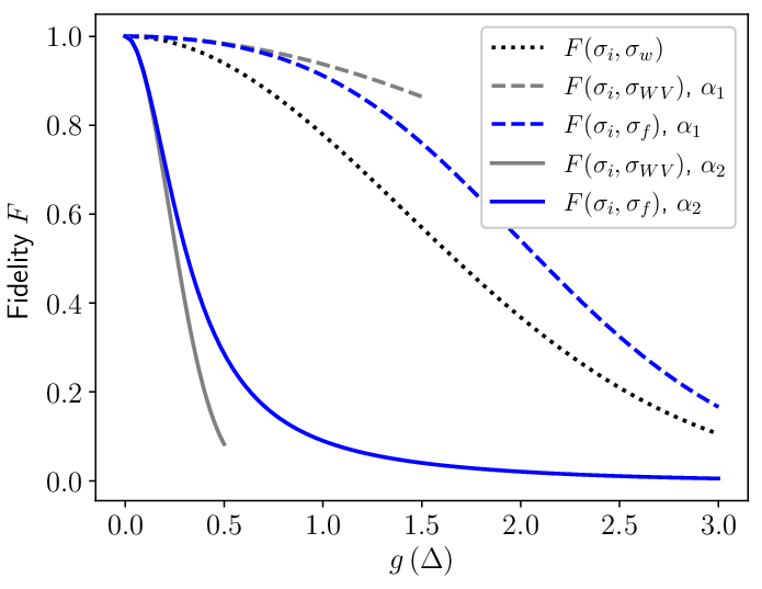
In Fig. 4 we show the fidelity (21) for increasing coupling strength $g$ and different preparation procedures $\alpha$. In the limit of $g\ll\Delta$ the fidelity of the WV measurement $F(\sigma_{i},\sigma_{WV})=\exp[-g^{2}\tan^{2}(\alpha/2)/(4\Delta^{2})]$ is recovered, but we can see that for larger coupling strength the WV is insufficient to describe the change of the pointer state and higher order terms need to be taken into account. In the projective measurement limit $g\gg\Delta$ the fidelity vanish. For comparison we have shown the fidelity without post-selection $F(\sigma_{i},\sigma_{w})=\exp[-g^{2}/(4\Delta^{2})]$.

However, we want to emphasize a feature of the pointer fidelity in relation to the performed post-selection. In Fig. 4 the fidelity between the initial state and the final state after post-selection $F(\sigma_{i},\sigma_{f})$ is larger than the fidelity without post-selection $F(\sigma_{i},\sigma_{w})$ for a preparation procedure with $\alpha_{1}=0.3\pi$, and in contrast $F(\sigma_{i},\sigma_{f})$ is smaller than $F(\sigma_{i},\sigma_{w})$ for the preparation angle $\alpha_{2}=0.9\pi$. The preparation procedure of the initial state $\rho_{i}(\alpha)$ has a larger overlap with the final post-selected state $\ket{\uparrow_x}$ for $\alpha_{1}$ or with the orthogonal state $\ket{\downarrow_x}$ for $\alpha_{2}$. Thus, for the case of $\bra{\downarrow_x}\rho_{i}(\alpha)\ket{\downarrow_x}\geq\bra{\uparrow_x}\rho_{i}(\alpha)\ket{\uparrow_x}$, the initial state $\rho_{i}(\alpha)$ and final state $\ket{\uparrow_x}$ tend to become orthogonal, leading to a larger WV and hence increased pointer shift. This ultimately reduce the fidelity $F(\sigma_{i},\sigma_{f})$. We shall now prove that this property is not accidental for the two angles shown, but holds for a general initial state $\ket{i}$ and final state $\ket{f}$ and corresponding orthogonal state $\ket{f_\perp}$. Essentially, we have to proof that

if $\absolutevalue{\braket{f_\perp}{i}}\geq\absolutevalue{\braket{f}{i}}$. Inserting the expressions for the fidelity we find that, $\cos\alpha\,e^{-g^{2}/(2\Delta^{2})}\geq\cos\alpha$. This is only true if $\cos\alpha\leq 0$, implying that $\alpha\in[{\pi}/{2},{3\pi}/{2}]$, which complete the proof. Note that this is the same region of initial states where the WV exceeds the eigenvalue range leading to anomalous pointer shifts.

We have seen that the outcome of a weak measurement including post-selection can cause the pointer state to shift almost arbitrarily large, leading to an enhancement effect for measuring the small coupling parameter $g$. This effect of large pointer shifts due to WV is used in the weak value amplification (WVA) technique, where a small signal can receive huge amplification effects due to post-selection hosten2008observation. This amplification is at the expense of a reduced post-selection probability for almost orthogonal initial and final states necessary to obtain large pointer shifts. Nevertheless, the WVA technique has been used to increase the measurement sensitivity of small effects in various experiments, and it was shown that WVA has an advantage in terms of quantum metrology by reducing different types of noise and making use of quantum resources hosten2008observation; dixon2009ultrasensitive; PhysRevLett.125.080501; starling2009optimizing; feizpour2011amplifying; dressel2013strengthening; jordan2014technical. Since the demonstrated advantage depends on the assumptions made about the experimental conditions, such as detector saturation or noise, there is still an ongoing debate under which conditions WVA can outperform a conventional measurement scheme brunner2010measuring; knee2013quantum; tanaka2013information; ferrie2014weak; knee2014amplification; zhang2015precision. However, considering realistic experimental conditions, e.g. including detector saturation and noise, it was conjectured vaidman2014comment and shown harris2017weak, that WVA can outperform conventional schemes, and can approach the quantum Cramér-Rao bound for parameter estimation pang2014entanglement; PhysRevLett.125.080501.

In the following we want to answer the question which measurement protocol provides the most unambiguous parameter detection, to extract the classical information? The larger the distinguishability between the initial $\sigma_{i}$ and final pointer state $\sigma_{f}$, the higher the probability to unambiguously correlate the measured pointer position to the previous interaction. Thus pointer readings are not mistakenly assigned to the interaction while the pointer is actually obtained from the initial position for large uncertainties. A measure to quantify this distinguishability between the pointer states is given by $1-F(\sigma_{i},\sigma_{f})$, implying that it is favorable to minimize the fidelity $F(\sigma_{i},\sigma_{f})$ in respect of increasing the unambiguous measurement detection.

In general, we observe, that the fidelity of the pointer between the initial and final state $F(\sigma_{i},\sigma_{f})$ is reduced for larger coupling strength and vanish for a projective measurement ($g\gg\Delta$). For moderate coupling strength $g\simeq\Delta$ the fidelity is reduced when an additional post-selection is performed on an almost orthogonal final state (see Fig. 4). Thus we assert that a conventional projective measurement is favorable in terms of an unambiguous retrodiction of the pointer shift. However, the conditions on the parameters ($g,\Delta$) are usually constraint by the experimental setup. And since the aim of WVA is to measure a very small parameter $g$, the constraint on $\Delta\ll g$ for projective measurements are severe. Thus, when taking into account this constraint imposed by the experimental setup the fidelity between initial and final pointer state is non-vanishing. Still pursuing for the least fidelity measure, we find that for an experiment with fixed $g\simeq\Delta$, the largest decrease of the fidelity $F(\sigma_{i},\sigma_{f})$ is observed when including post-selection on almost orthogonal initial and final states, precisely the requirements of anomalous WV (Fig. 4). We thus observe, that under the possible constraint imposed by the experiment, a weak measurement protocol including post-selection lead to the largest detection sensitivity of the small coupling parameter $g$.

Note that a weak measurement alone does not lead to a pronounced decrease of the fidelity and only in combination with a post-selection on an orthogonal state a significant decrease of the fidelity is observed. Thus the unambiguous differentiation between the pointer state before and after the measurement protocol is enhanced by a proper post-selection, in accordance with the observed increase of quantum Fisher information for post-selected weak measurements compared to weak measurements alone pang2015improving.

To quantify the measurement sensitivity of the extracted information from the pointer perspective, we will make use of the pointer fidelity. The fidelity for the pointer state imply that more information about the observable is extracted for lower values, in the sense that it makes the outcome more distinguishable from the initial state. We thus want to place an upper bound on the pointer fidelity $F_{b}$, such that information about the interaction can unambiguously obtained. Since the fidelity reduces for larger coupling strength, we deduce the minimum coupling strength $g_{min}$, in order to obtain $F_{b}$ for the different measurement protocols.

For a weak measurement without post-selection with $F_{b}(\sigma_{i},\sigma_{w})=\exp[-g^{2}/(4\Delta^{2})]$, we readily found that $g_{min}^{I}=2\Delta\sqrt{\absolutevalue{\ln F_{b}}}$. However, if we perform a subsequent post-selection on the system we can solve (21) for $g_{min}$ and obtain

where $C(\alpha)=1+\cos\alpha$. We can now compare the arguments of the square root from $g_{min}^{I}$, and $g_{min}^{II}$, to identify the regime in which the coupling strength is minimized by the post-selection procedure. Assuming that $g_{min}^{II}\leq g_{min}^{I}$, imply that, $\ln F_{b}\leq-\ln[\kappa(\alpha)/(2F_{b})]$, where $\kappa(\alpha)=C(\alpha)+\sqrt{C(\alpha)^{2}-4F_{b}^{2}\cos\alpha}$. This holds only when $\cos\alpha\leq 0$, i.e. $\alpha\in[\pi/2,3\pi/2]$. Thus, in the regime when initial and final state become orthogonal, then the post-selection procedure can improve the measurement sensitivity. This is to be understood in terms of obtaining the same pointer fidelity $F_{b}$ as in the case without post-selection for a smaller coupling strength $g_{min}^{II}\leq g_{min}^{I}$.

If we insert these lower bounds for the coupling strength into the trace distance of the system states of Eq. (13), we have a quantitative measure for the actual state disturbance after the intermediate weak measurement. We find that for the weak measurement case without post-selection

Using the relation between trace distance and fidelity $D(\sigma_{1},\sigma_{2})\leq\sqrt{1-F(\sigma_{1},\sigma_{2})^{2}}$ fuchs1999cryptographic, we obtain a lower bound on the state disturbance of the system with respect to the trace distance of the pointer $D_{p}(\sigma_{i},\sigma_{w})$

This is the trade-off relation for the state disturbance of the system state in terms of the pointer state change.

However, performing an additional post-selection the minimal coupling strength needed to obtain the same pointer fidelity $F_{b}$ is different. Using (13) and (23) we find for the minimal state disturbance

where $\gamma(\alpha)=4/\kappa^{2}(\alpha)$. If $\gamma(\alpha)\geq 1$ the distinguishability between the initial state and the state following the weak measurement is decreased compared to the non-post-selection scenario (24). We found that $\gamma(\alpha)=4/\kappa^{2}(\alpha)\geq 1$, if $\cos\alpha\leq 0$, which is the case for $\alpha\in[\pi/2,3\pi/2]$, and thus $D_{min}^{II}(\rho_{i},\rho_{w})\leq D_{min}^{I}(\rho_{i},\rho_{w})$. Hence, a reduced state disturbance due to post-selection is given for the same initial preparation where we obtain anomalous large WV and a reduced pointer fidelity. The state disturbance of (24) and (26) can be seen in Fig. 5, where a considerably large advantage in terms of a reduced disturbance due to post-selection can be found for the case of $\alpha_{3}=0.9\pi$ (solid). Note that technically the post-selection itself not reduces the system state disturbance in the sense that it cures a previous larger disturbance, but it allows to operate the experiment with a coupling strength $g_{min}$ smaller than for the case without post-selection in order to reach the same fidelity for the pointer state $F_{b}$.

This observation is in accordance with the advantage of the weak value amplification technique for small coupling strength. If we wish to measure a small coupling parameter $g$ the measurement sensitivity of the pointer can considerably increase if a post-selection on a system state orthogonal to the initial state is performed.

We have seen, that it is necessary to disturb the system in order to extract any information from it fuchs1996quantum; fuchs1998information; fuchs2001information, whereas the disturbance of the system in a WV measurement protocol is often neglected aharonov1990properties. Thus, it is assumed that $D(\rho_{i},\rho_{w})\simeq 0$. Given the lower bound of the coupling strength $g_{min}$ for a desired pointer fidelity, we can ask the question whether the disturbance of the weak measurement is actually negligible or not?

The disturbance of the system for the coupling strength $g_{min}$, needed to obtain the pointer fidelity $F_{b}$, is given by $D_{min}^{II}(\rho_{i},\rho_{w})$ (Eq. (26)) and $D_{min}^{I}(\rho_{i},\rho_{w})$ (Eq. (24)), for the case with and without post-selection, respectively. For realistic experimental conditions with an initial state of angle $\alpha=170^{\circ}$ and post-selecting for $\beta=0$, we found that the state disturbance for a pointer fidelity of $F_{b}=0.1$ is given by $D_{min}^{II}(\rho_{i},\rho_{w})=0.06$. And depending on the desired task, this disturbance can be considered as negligible. However, here we have used that following the weak measurement a post-selection on the system is performed such that the minimal coupling strength can be reduced to obtain the same pointer fidelity as opposed to the case of a single weak measurement with-out post-selection in which $g_{min}^{I}\geq g_{min}^{II}$. Consequently the disturbance for the case without post-selection for the same experimental conditions, is $D_{min}^{I}(\rho_{i},\rho_{w})=0.49$, and can by no means neglected.

Thus, for the measurement protocol including post-selection, which can operate with a smaller coupling strength to obtain the same detection sensitivity, we found that the disturbance due to the intermediate weak measurement can be neglected. In contrast, a single weak measurement without post-selection will significantly disturb the system to reach the equivalent measurement sensitivity.

Important for anomalous WV measurements is that the initial $\ket{i}=\cos\alpha/2\ket{\uparrow_x}+\sin\alpha/2\ket{\downarrow_x}$, and final $\ket{f}=\ket{\uparrow_x}$ state need to be almost orthogonal, resulting in a reduced signal intensity due to post-selection. Since the state disturbance during the weak measurement is usually neglected, the success probability of the post-selection measurement outcomes is likewise approximated by $P_{ap}=\absolutevalue{\bra{f}\ket{i}}^{2}=\absolutevalue{\cos{\alpha}/{2}}^{2}$, whereas the exact post-selection probability (7) is given by, $P_{f}=\frac{1}{2}(1+\cos\alpha\,\exp[-g^{2}/(2\Delta^{2})])$. For the experimental parameters from above with $g_{min}^{II}$ from (23), we found that $P_{ap}=0.0076$, but for the exact post-selection probability we have $P_{f}=0.071$, which exceed the approximated post-selection probability by nearly one order of magnitude. The fact that the exact post-selection probability is considerably larger than the approximated overlap of initial and final state, provides further advantage for the weak value amplification technique in the sense that the true number of counts is much larger than often assumed.

References

- [1] R. P. Feynman. Space-time approach to non-relativistic quantum mechanics. Rev. Mod. Phys., 20:367–387, Apr 1948.
- [2] Asher Peres. Quantum theory: concepts and methods, volume 57. Springer Science & Business Media, 2006.
- [3] Johann v Neumann. Mathematische grundlagen der quantenmechanik, volume 38. Springer-Verlag, 2013.
- [4] Gerhart Lüders. Über die zustandsänderung durch den meßprozeß. Annalen der Physik, 443(5-8):322–328, 1950.
- [5] Yakir Aharonov, Peter G Bergmann, and Joel L Lebowitz. Time symmetry in the quantum process of measurement. Physical Review, 134(6B):B1410, 1964.
- [6] Howard M Wiseman and Gerard J Milburn. Quantum measurement and control. Cambridge university press, 2009.
- [7] Yakir Aharonov, David Z Albert, and Lev Vaidman. How the result of a measurement of a component of the spin of a spin-1/2 particle can turn out to be 100. Physical review letters, 60(14):1351, 1988.
- [8] NWM Ritchie, J Greg Story, and Randall G Hulet. Realization of a measurement of a “weak value”. Physical review letters, 66(9):1107, 1991.
- [9] IM Duck, Paul M Stevenson, and ECG Sudarshan. The sense in which a” weak measurement” of a spin- particle’s spin component yields a value 100. Physical Review D, 40(6):2112, 1989.
- [10] HM Wiseman. Weak values, quantum trajectories, and the cavity-qed experiment on wave-particle correlation. Physical Review A, 65(3):032111, 2002.
- [11] Justin Dressel, Mehul Malik, Filippo M Miatto, Andrew N Jordan, and Robert W Boyd. Colloquium: Understanding quantum weak values: Basics and applications. Reviews of Modern Physics, 86(1):307, 2014.
- [12] Lev Vaidman. Weak value controversy. Philosophical Transactions of the Royal Society A: Mathematical, Physical and Engineering Sciences, 375(2106):20160395, 2017.
- [13] Aephraim M Steinberg. How much time does a tunneling particle spend in the barrier region? Physical review letters, 74(13):2405, 1995.
- [14] Nathan S Williams and Andrew N Jordan. Weak values and the leggett-garg inequality in solid-state qubits. Physical review letters, 100(2):026804, 2008.
- [15] R Mir, JS Lundeen, MW Mitchell, AM Steinberg, JL Garretson, and HM Wiseman. A double-slit ‘which-way’experiment on the complementarity–uncertainty debate. New Journal of Physics, 9(8):287, 2007.
- [16] AP Lund and HM Wiseman. Measuring measurement–disturbance relationships with weak values. New Journal of Physics, 12(9):093011, 2010.
- [17] Sacha Kocsis, Boris Braverman, Sylvain Ravets, Martin J Stevens, Richard P Mirin, L Krister Shalm, and Aephraim M Steinberg. Observing the average trajectories of single photons in a two-slit interferometer. Science, 332(6034):1170–1173, 2011.
- [18] Lee A Rozema, Ardavan Darabi, Dylan H Mahler, Alex Hayat, Yasaman Soudagar, and Aephraim M Steinberg. Violation of heisenberg’s measurement-disturbance relationship by weak measurements. Physical review letters, 109(10):100404, 2012.
- [19] AK Pan. Interference experiment, anomalous weak value, and leggett-garg test of macrorealism. Physical Review A, 102(3):032206, 2020.
- [20] Jeff S Lundeen and Aephraim M Steinberg. Experimental joint weak measurement on a photon pair as a probe of hardy’s paradox. Physical review letters, 102(2):020404, 2009.
- [21] Yakir Aharonov, Alonso Botero, Shmuel Nussinov, Sandu Popescu, Jeff Tollaksen, and Lev Vaidman. The classical limit of quantum optics: not what it seems at first sight. New Journal of Physics, 15(9):093006, 2013.
- [22] Ariel Danan, Demitry Farfurnik, Shimshon Bar-Ad, and Lev Vaidman. Asking photons where they have been. Physical review letters, 111(24):240402, 2013.
- [23] C Aris Chatzidimitriou-Dreismann. Weak values and two-state vector formalism in elementary scattering and reflectivity—a new effect. Universe, 5(2):58, 2019.
- [24] Jeff S Lundeen, Brandon Sutherland, Aabid Patel, Corey Stewart, and Charles Bamber. Direct measurement of the quantum wavefunction. Nature, 474(7350):188–191, 2011.
- [25] Jeff S Lundeen and Charles Bamber. Procedure for direct measurement of general quantum states using weak measurement. Physical review letters, 108(7):070402, 2012.
- [26] Guillaume S Thekkadath, Lambert Giner, Yamn Chalich, Matthew J Horton, Jash Banker, and Jeff S Lundeen. Direct measurement of the density matrix of a quantum system. Physical review letters, 117(12):120401, 2016.
- [27] Shengjun Wu. State tomography via weak measurements. Scientific reports, 3:1193, 2013.
- [28] Liang Xu, Huichao Xu, Feixiang Xu, Kaimin Zheng, and Lijian Zhang. Direct characterization of quantum measurement using weak values. arXiv preprint arXiv:2005.10423, 2020.
- [29] P Ben Dixon, David J Starling, Andrew N Jordan, and John C Howell. Ultrasensitive beam deflection measurement via interferometric weak value amplification. Physical review letters, 102(17):173601, 2009.
- [30] Holger F Hofmann. Uncertainty limits for quantum metrology obtained from the statistics of weak measurements. Physical Review A, 83(2):022106, 2011.
- [31] Liang Xu, Zexuan Liu, Animesh Datta, George C. Knee, Jeff S. Lundeen, Yan-qing Lu, and Lijian Zhang. Approaching quantum-limited metrology with imperfect detectors by using weak-value amplification. Phys. Rev. Lett., 125:080501, Aug 2020.
- [32] Christopher A Fuchs. Information gain vs. state disturbance in quantum theory. Fortschritte der Physik: Progress of Physics, 46(4-5):535–565, 1998.
- [33] Christopher A Fuchs and Asher Peres. Quantum-state disturbance versus information gain: Uncertainty relations for quantum information. Physical Review A, 53(4):2038, 1996.
- [34] Christopher A Fuchs and Kurt Jacobs. Information-tradeoff relations for finite-strength quantum measurements. Physical Review A, 63(6):062305, 2001.
- [35] Yakir Aharonov and Lev Vaidman. Properties of a quantum system during the time interval between two measurements. Physical Review A, 41(1):11, 1990.
- [36] Maximilian Schlosshauer. Analysis of quantum-state disturbance in a protective measurement of a spin-1/2 particle. Physical Review A, 92(6):062116, 2015.
- [37] Asger C Ipsen. Disturbance in weak measurements and the difference between quantum and classical weak values. Physical Review A, 91(6):062120, 2015.
- [38] Saki Tanaka and Naoki Yamamoto. Information amplification via postselection: A parameter-estimation perspective. Physical Review A, 88(4):042116, 2013.
- [39] George C Knee and Erik M Gauger. When amplification with weak values fails to suppress technical noise. Physical Review X, 4(1):011032, 2014.
- [40] Lijian Zhang, Animesh Datta, and Ian A Walmsley. Precision metrology using weak measurements. Physical review letters, 114(21):210801, 2015.
- [41] Jérémie Harris, Robert W Boyd, and Jeff S Lundeen. Weak value amplification can outperform conventional measurement in the presence of detector saturation. Physical review letters, 118(7):070802, 2017.
- [42] Igor D Ivanovic. How to differentiate between non-orthogonal states. Physics Letters A, 123(6):257–259, 1987.
- [43] Asher Peres. How to differentiate between non-orthogonal states. Physics Letters A, 128(1-2):19, 1988.
- [44] AW Bray, U Eichmann, and S Patchkovskii. Dissecting strong-field excitation dynamics with atomic-momentum spectroscopy. Physical Review Letters, 124(23):233202, 2020.
- [45] Xuanmin Zhu, Yuxiang Zhang, Shengshi Pang, Chang Qiao, Quanhui Liu, and Shengjun Wu. Quantum measurements with preselection and postselection. Physical Review A, 84(5):052111, 2011.
- [46] Richard Jozsa. Complex weak values in quantum measurement. Physical Review A, 76(4):044103, 2007.
- [47] Justin Dressel. Weak values as interference phenomena. Physical Review A, 91(3):032116, 2015.
- [48] Fixing the angle does not change the behaviour of the measurement outcomes as long as , where is an eigenstate of .
- [49] Christopher A Fuchs and Jeroen Van De Graaf. Cryptographic distinguishability measures for quantum-mechanical states. IEEE Transactions on Information Theory, 45(4):1216–1227, 1999.
- [50] Michael A Nielsen and Isaac Chuang. Quantum computation and quantum information, 2002.
- [51] Lev Vaidman, Alon Ben-Israel, Jan Dziewior, Lukas Knips, Mira Weißl, Jasmin Meinecke, Christian Schwemmer, Ran Ber, and Harald Weinfurter. Weak value beyond conditional expectation value of the pointer readings. Physical Review A, 96(3):032114, 2017.
- [52] Onur Hosten and Paul Kwiat. Observation of the spin hall effect of light via weak measurements. Science, 319(5864):787–790, 2008.
- [53] David J Starling, P Ben Dixon, Andrew N Jordan, and John C Howell. Optimizing the signal-to-noise ratio of a beam-deflection measurement with interferometric weak values. Physical Review A, 80(4):041803, 2009.
- [54] Amir Feizpour, Xingxing Xing, and Aephraim M Steinberg. Amplifying single-photon nonlinearity using weak measurements. Physical review letters, 107(13):133603, 2011.
- [55] Justin Dressel, Kevin Lyons, Andrew N Jordan, Trent M Graham, and Paul G Kwiat. Strengthening weak-value amplification with recycled photons. Physical Review A, 88(2):023821, 2013.
- [56] Andrew N Jordan, Julián Martínez-Rincón, and John C Howell. Technical advantages for weak-value amplification: when less is more. Physical Review X, 4(1):011031, 2014.
- [57] Nicolas Brunner and Christoph Simon. Measuring small longitudinal phase shifts: weak measurements or standard interferometry? Physical review letters, 105(1):010405, 2010.
- [58] George C Knee, G Andrew D Briggs, Simon C Benjamin, and Erik M Gauger. Quantum sensors based on weak-value amplification cannot overcome decoherence. Physical Review A, 87(1):012115, 2013.
- [59] Christopher Ferrie and Joshua Combes. Weak value amplification is suboptimal for estimation and detection. Physical review letters, 112(4):040406, 2014.
- [60] L Vaidman. Comment on” weak value amplification is suboptimal for estimation and detection”. arXiv preprint arXiv:1402.0199, 2014.
- [61] Shengshi Pang, Justin Dressel, and Todd A Brun. Entanglement-assisted weak value amplification. Physical Review Letters, 113(3):030401, 2014.
- [62] Shengshi Pang and Todd A Brun. Improving the precision of weak measurements by postselection measurement. Physical review letters, 115(12):120401, 2015.
- [63] Yong Wook Cheong and Seung-Woo Lee. Balance between information gain and reversibility in weak measurement. Physical review letters, 109(15):150402, 2012.
- [64] Longfei Fan, Wenchao Ge, Hyunchul Nha, and M Suhail Zubairy. Trade-off between information gain and fidelity under weak measurements. Physical Review A, 92(2):022114, 2015.
- [65] David RM Arvidsson-Shukur, Nicole Yunger Halpern, Hugo V Lepage, Aleksander A Lasek, Crispin HW Barnes, and Seth Lloyd. Quantum negativity provides advantage in postselected metrology. arXiv preprint arXiv:1903.02563, 2019.
- [66] Yaron Kedem. Using technical noise to increase the signal-to-noise ratio of measurements via imaginary weak values. Physical Review A, 85(6):060102, 2012.
- [67] DA Ivanov, T Yu Ivanova, SF Caballero-Benitez, and IB Mekhov. Feedback-induced quantum phase transitions using weak measurements. Physical Review Letters, 124(1):010603, 2020.
- [68] Maximilian Schlosshauer. Protective measurement of open quantum systems. Physical Review A, 101(1):012108, 2020.
- [69] Hammad Anwer, Sadiq Muhammad, Walid Cherifi, Nikolai Miklin, Armin Tavakoli, and Mohamed Bourennane. Experimental characterization of unsharp qubit observables and sequential measurement incompatibility via quantum random access codes. Physical Review Letters, 125(8):080403, 2020.