跳到论文正文
W Papers独立论文阅读器 arXiv:2011.04253 论文正文 计算阅读时间 · 0%
引用这篇论文根据当前论文元数据生成,正式投稿前建议核对。


License: CC BY 4.0
arXiv:2011.04253v2 [cs.CC] 09 Feb 2023

Machinery for Proving Sum-of-Squares Lower Bounds on Certification Problems

Aaron Potechin Thanks: University of Chicago. potechin@uchicago.edu. Supported in part by NSF grant CCF-2008920.    Goutham Rajendran Thanks: University of Chicago. goutham@uchicago.edu. Supported in part by NSF grants CCF-1816372 and CCF-2008920.
August 11, 2026
Abstract

In this paper, we construct general machinery for proving Sum-of-Squares lower bounds on certification problems by generalizing the techniques used by Barak et al. [BHK+16] to prove Sum-of-Squares lower bounds for planted clique. Using this machinery, we prove degree nεn^{\varepsilon} Sum-of-Squares lower bounds for tensor PCA, the Wishart model of sparse PCA, and a variant of planted clique which we call planted slightly denser subgraph.

1 Introduction

The Sum-of-Squares (SoS) hierarchy is an optimization technique that harnesses the power of semidefinite programming to solve optimization tasks. First independently investigated by Shor [Sho87], Nesterov [Nes00], Parillo [Par00], Lasserre [Las01] and Grigoriev [Gri01a, Gri01b], the SoS hierarchy offers a sequence of convex relaxations for polynomial optimization problems and is parameterized by an integer called the degree of the SoS hierarchy. As we increase the degree dd of the hierarchy, we get progressively stronger convex relaxations which are solvable in nO⁡(d)n^{O(d)} time11 1 There is a caveat, see [O’D17]. This has paved the way for the SoS hierarchy to be a powerful tool in algorithm design both in the worst case and the average case settings. Indeed, there has been tremendous success in using the SoS hierarchy to obtain efficient algorithms for combinatorial optimization problems (e.g., [GW95, ARV04, GS11, RRS17]) as well as problems stemming from Statistics and Machine Learning (e.g., [BBH+12, BKS15, HSS15, PS17, KS17]). In fact, SoS achieves the state-of-the-art approximation guarantees for many fundamental problems such as Sparsest Cut [ARV04], MaxCut [GW95], Tensor PCA [HSS15] and all Max-kk-CSPs [Rag08]. Moreover, for a large class of problems, it’s been shown that SoS relaxations are the most efficient among all semidefinite programming relaxations [LRS15].

On the flip side, some problems have remained intractable beyond a certain threshold even by considering higher degrees of the SoS hierarchy [BHK+16, KMOW17, MRX20, GJJ+20]. For example, consider the Planted Clique problem where we have to distinguish a random graph sampled from the Erdős-Rényi model G⁡(n,12)G(n,\frac{1}{2}) from a random graph which is obtained by first sampling a graph from G⁡(n,12)G(n,\frac{1}{2}) and then planting a clique of size n12−εn^{\frac{1}{2}-\varepsilon} for a small constant ε>0\varepsilon>0. It was shown in [BHK+16] that with high probability degree o⁡(log⁡n)o(\log n) SoS fails to solve this distinguishing problem.

There are many reasons for why studying lower bounds against the SoS hierarchy is important. Firstly, SoS is a generic proof system that captures a broad class of algorithmic reasoning [FKP19]. In particular, under mild conditions, SoS captures statistical query algorithms and algorithms based on low degree polynomials. Therefore, SoS lower bounds indicate to the algorithm designer the intrinsic hardness of the problem and suggest that if they want to break the algorithmic barrier, they need to search for algorithms that are not captured by SoS. Secondly, in average case problem settings, standard complexity theoretic assumptions such as P ≠\neq NP have not been shown to give insight into the limits of efficient algorithms. Instead, lower bounds against powerful proof systems such as SoS have served as strong evidence of computational hardness [HKP+17, Hop18, Kun21]. Thus, understanding the power of the SoS hierarchy on these problems is an important step towards understanding the approximability of these problems.

1.1 Our contributions

In this paper, we consider the following general category of problems: Given a random input, can we certify that it does not contain a given structure? Some important examples of this kind of problem are as follows.

  1. 1.

    Planted clique: Can we certify that a random graph does not have a large clique?

  2. 2.

    Tensor PCA: Given an order kk tensor TT with random independent Gaussian entries, can we certify that there is no unit vector xx such that ⟨T,x⊗…⊗x⟩\langle T,x\otimes\ldots\otimes x\rangle is large?

  3. 3.

    Wishart model of sparse PCA: Given an m×dm\times d matrix SS with random independent Gaussian entries (which corresponds to taking mm samples from 𝒩⁡(0,Id)\mathcal{N}(0,I_{d})), can we certify that there is no kk-sparse unit vector xx such that ‖S​x‖\left\lVert Sx\right\rVert is large?

These kinds of problems, known as certification problems, are closely related to their optimization or estimation variants. A certification algorithm is required to produce a proof/certificate of a bound that holds for all inputs, as opposed to most inputs. The Sum-of-Squares hierarchy provides such certificates in a canonical way for a wide variety of such problems, so analyzing SoS paves the way towards understanding the certification complexity of these problems. We investigate the following question.

For certification problems, what are the best bounds that SoS can certify?

In this work, we build general machinery for proving probabilistic Sum of Squares lower bounds on certification problems. To build our machinery, we generalize the techniques pioneered by [BHK+16] for proving Sum of Squares lower bounds for planted clique. We start with the standard framework for proving probabilistic Sum of Squares lower bounds:

  1. 1.

    Construct candidate pseudo-expectation values 𝔼~\tilde{\mathop{\mathbb{E}}} and the corresponding moment matrix Λ\Lambda (see Section 2.1).

  2. 2.

    Show that with high probability, Λ⪰0\Lambda\succeq 0.

For planted clique, [BHK+16] constructed 𝔼~\tilde{\mathop{\mathbb{E}}} and the corresponding moment matrix Λ\Lambda by introducing the pseudo-calibration technique (see Section 2.2). They then showed through a careful and highly technical analysis that with high probability Λ⪰0\Lambda\succeq 0.

In this paper, we investigate how generally the techniques used for planted clique can be applied. We show that by considering coefficient matrices based on the coefficients obtained by pseudo-calibration, we can give a general framework which captures most of the technical analysis for the sum of squares lower bound for planted clique [BHK+16]. Using this framework, we show that there are relatively simple conditions on these coefficient matrices which are sufficient to ensure that the moment matrix Λ\Lambda is PSD with high probability. This allows us to focus on the structure which is specific to each problem rather than the technical details of the analysis.

We exhibit the usefulness of our machinery by using it to achieve strong SoS lower bounds for the problems of Tensor PCA, Sparse PCA and a problem closely related to the Planted Clique problem that we call Planted Slightly Denser Subgraph. We do this with relative ease once the machinery is in place. The Sparse PCA lower bounds complement a long line of work on algorithmic guarantees that stretches for over two decades (the most recent one being [dKNS20]), thereby giving a complete picture (up to polylogarithmic factors) for the approximability-inapproximability thresholds for Sparse PCA.

We believe that our machinery is a promising approach for proving a variant of the low-degree conjecture (see [Hop18, HW20] for background on the low-degree conjecture). The low-degree conjecture is a fascinating open problem which says if there is a low-degree polynomial lower bound for a problem which is sufficiently symmetric then there is a sum of squares lower bound for a noisy version of the problem. If we can show that having a low-degree polynomial lower bound implies that the coefficient matrices obtained via pseudo-calibration (for the noisy version of the problem) obey the conditions required for our machinery, then this would prove this variant of the low-degree conjecture.

1.1.1 A brief summary of pseudo-calibration

A natural way to prove lower bounds on a certification problem is as follows.

  1. 1.

    Construct a “maximum entropy” planted distribution of inputs which has the given structure.

  2. 2.

    Show that we cannot distinguish between the random and planted distributions and thus cannot certify that a random input does not have the given structure.

Based on this idea, the pseudo-calibration technique introduced by [BHK+16] constructs candidate pseudo-expectation values 𝔼~\tilde{\mathop{\mathbb{E}}} so that as far as low degree tests are concerned, 𝔼~\tilde{\mathop{\mathbb{E}}} for the random distribution mimics the behavior of the given structure for the planted distribution (for details, see Section 2.2). This gives a candidate moment matrix Λ\Lambda which we can then analyze with our machinery. A majority of known high-degree average-case SoS lower bounds in the literature have pseudo-expectation values that were either obtained by, or could be obtained by pseudocalibration, e.g., Planted Clique [BHK+16], Max-kk-CSPs [KMOW17], Max-Cut on regular graphs [MRX20], Sherrington-Kirkpatrick problem [GJJ+20, MRX20]. It has also been successful for Densest-kk-subgraph but for the weaker Sherali-Adams Hierarchy [CM18].

Naturally, pseudocalibration is the starting point for our SoS lower bounds. That said, our machinery is quite general and can be applied even if the candidate moment matrix Λ\Lambda is not obtained via pseudo-calibration.

1.1.2 Our results on Tensor PCA, Sparse PCA, and Planted Slightly Denser Subgraph

In this section, we formally state the main hardness theorems we show by applying our machinery. We defer discussing prior work, how we improve on them, and other related work to Section 1.2.

We describe the planted distributions we use to show our SoS lower bounds for planted slightly denser subgraph, tensor PCA, and the the Wishart model of sparse PCA. We also state the random distributions for completeness and for contrast. We then state our results.

Planted slightly denser subgraph

We use the following distributions.

  • []

  • -

    Random distribution: Sample GG from G⁡(n,12)G(n,\frac{1}{2})

  • -

    Planted distribution: Let kk be an integer and let p>12p>\frac{1}{2}. Sample a graph G′G^{\prime} from G⁡(n,12)G(n,\frac{1}{2}). Choose a random subset SS of the vertices, where each vertex is picked independently with probability kn\frac{k}{n}. For all pairs i,ji,j of vertices in SS, rerandomize the edge (i,j)(i,j) where the probability of (i,j)(i,j) being in the graph is now pp. Set GG to be the resulting graph.

In Section 4, we compute the candidate moment matrix Λ\Lambda obtained by pseudo-calibration.

Theorem 1.1.

Let Cp>0C_{p}>0. There exists a constant C>0C>0 such that for all sufficiently small constants ε>0\varepsilon>0, if k≤n12−εk\leq n^{\frac{1}{2}-\varepsilon} and p=12+n−Cp​ε2p=\frac{1}{2}+\frac{n^{-C_{p}\varepsilon}}{2}, then with high probability, the candidate moment matrix Λ\Lambda given by pseudo-calibraton for degree nC​εn^{C\varepsilon} Sum-of-Squares is PSD.

Corollary 1.2.

Let Cp>0C_{p}>0. There exists a constant C>0C>0 such that for all sufficiently small constants ε>0\varepsilon>0, if k≤n12−εk\leq n^{\frac{1}{2}-\varepsilon} and p=12+n−Cp​ε2p=\frac{1}{2}+\frac{n^{-C_{p}\varepsilon}}{2}, then with high probability, degree nC​εn^{C\varepsilon} Sum-of-Squares cannot certify that a random graph GG from G⁡(n,12)G(n,\frac{1}{2}) does not have a subgraph of size ≈k\approx k with edge density ≈p\approx p.

Tensor PCA

Let k≥2k\geq 2 be an integer. We use the following distributions.

  • []

  • -

    Random distribution: Sample AA from 𝒩⁡(0,I[n]k)\mathcal{N}(0,I_{[n]^{k}}).

  • -

    Planted distribution: Let λ,Δ>0\lambda,\Delta>0. Sample uu from {−1Δ​n,0,1Δ​n}n\{-\frac{1}{\sqrt{\Delta n}},0,\frac{1}{\sqrt{\Delta n}}\}^{n} where the values are taken with probabilites Δ2,1−Δ,Δ2\frac{\Delta}{2},1-\Delta,\frac{\Delta}{2} respectively. Then sample BB from 𝒩⁡(0,I[n]k)\mathcal{N}(0,I_{[n]^{k}}). Set A=B+λ​u⊗kA=B+\lambda u^{\otimes k}.

In Section 5, we compute the candidate moment matrix Λ\Lambda obtained by pseudo-calibration.

Theorem 1.3.

Let k≥2k\geq 2 be an integer. There exist constants C,CΔ>0C,C_{\Delta}>0 such that for all sufficiently small constants ε>0\varepsilon>0, if λ≤nk4−ε\lambda\leq n^{\frac{k}{4}-\varepsilon} and Δ=n−CΔ​ε\Delta=n^{-C_{\Delta}\varepsilon} then with high probability, the candidate moment matrix Λ\Lambda given by pseudo-calibration for degree nC​εn^{C\varepsilon} Sum-of-Squares is PSD.

Corollary 1.4.

Let k≥2k\geq 2 be an integer. There exists a constant C>0C>0 such that for all sufficiently small constants ε>0\varepsilon>0, if λ≤nk4−ε\lambda\leq n^{\frac{k}{4}-\varepsilon}, then with high probability, degree nC​εn^{C\varepsilon} Sum-of-Squares cannot certify that for a random tensor AA from 𝒩⁡(0,I[n]k)\mathcal{N}(0,I_{[n]^{k}}), there is no vector uu such that ‖u‖≈1\left\lVert u\right\rVert\approx 1 and ⟨A,u⊗…⊗u⏟k times⟩≈λ\langle A,\underbrace{u\otimes\ldots\otimes u}_{\text{k times}}\rangle\approx\lambda.

Wishart model of Sparse PCA

We use the following distributions.

  • []

  • -

    Random distribution: v1,…,vmv_{1},\ldots,v_{m} are sampled from 𝒩⁡(0,Id)\mathcal{N}(0,I_{d}) and we take SS to be the m×dm\times d matrix with rows v1,…,vmv_{1},\ldots,v_{m}.

  • -

    Planted distribution: Sample uu from {−1k,0,1k}d\{-\frac{1}{\sqrt{k}},0,\frac{1}{\sqrt{k}}\}^{d} where the values are taken with probabilites k2​d,1−kd,k2​d\frac{k}{2d},1-\frac{k}{d},\frac{k}{2d} respectively. Then sample v1,…,vmv_{1},\ldots,v_{m} as follows. For each i∈[m]i\in[m], with probability Δ\Delta, sample viv_{i} from 𝒩⁡(0,Id+λ​u​uT)\mathcal{N}(0,I_{d}+\lambda uu^{T}) and with probability 1−Δ1-\Delta, sample viv_{i} from 𝒩⁡(0,Id)\mathcal{N}(0,I_{d}). Finally, take SS to be the m×dm\times d matrix with rows v1,…,vmv_{1},\ldots,v_{m}.

In Section 6, we compute the candidate moment matrix Λ\Lambda obtained by pseudo-calibration.

Theorem 1.5.

There exists a constant C>0C>0 such that for all sufficiently small constants ε>0\varepsilon>0, if m≤d1−ελ2,m≤k2−ελ2m\leq\frac{d^{1-\varepsilon}}{\lambda^{2}},m\leq\frac{k^{2-\varepsilon}}{\lambda^{2}}, and there exists a constant AA such that 0<A<140<A<\frac{1}{4}, d4​A≤k≤d1−A​εd^{4A}\leq k\leq d^{1-A\varepsilon}, and λk≤d−A​ε\frac{\sqrt{\lambda}}{\sqrt{k}}\leq d^{-A\varepsilon}, then with high probability, the candidate moment matrix Λ\Lambda given by pseudo-calibration for degree dC​εd^{C\varepsilon} Sum-of-Squares is PSD.

Corollary 1.6.

There exists a constant C>0C>0 such that for all sufficiently small constants ε>0\varepsilon>0, if m≤d1−ελ2,m≤k2−ελ2m\leq\frac{d^{1-\varepsilon}}{\lambda^{2}},m\leq\frac{k^{2-\varepsilon}}{\lambda^{2}}, and there exists a constant AA such that 0<A<140<A<\frac{1}{4}, d4​A≤k≤d1−A​εd^{4A}\leq k\leq d^{1-A\varepsilon}, and λk≤d−A​ε\frac{\sqrt{\lambda}}{\sqrt{k}}\leq d^{-A\varepsilon}, then with high probability, the degree dC​εd^{C\varepsilon} degree Sum-of-Squares cannot certify that for a random m×dm\times d matrix SS with Gaussian entries, there is no vector uu such that uu has ≈k\approx k nonzero entries, ‖u‖≈1\left\lVert u\right\rVert\approx 1, and ‖S​u‖2≈m+m​Δ​λ\left\lVert Su\right\rVert^{2}\approx m+m{\Delta}\lambda.

Remark 1.7.

Note that our planted distributions only approximately satisfy constraints such as having a subgraph of size kk, having a unit vector uu, and having uu be kk-sparse. While we would like to use planted distributions which satisfy such constraints exactly, these distributions bring additional technical difficulties. This same issue appeared in the SoS lower bounds for planted clique [BHK+16], which was recently resolved by Pang [Pan21]. Resolving this issue in general is a subtle but important open problem.

1.2 Relation to prior work on Planted Clique/Dense Subgraph, Tensor PCA, and Sparse PCA

1.2.1 Planted Dense Subgraph

In the planted dense subgraph problem, we are given a random graph GG where a dense subgraph of size kk has been planted and we are asked to find this planted dense subgraph. This is a natural generalization of the kk-clique problem [Kar72] and has been subject to a long line of work over the years (e.g. [FS+97, FPK01, Kho06, BCC+10, BCG+12, BKRW17, Man17]). In this work, we consider the following certification variant of planted dense subgraph.

Given a random graph GG sampled from the Erdős-Rényi model G⁡(n,12)G(n,\frac{1}{2}), certify an upper bound on the edge density of the densest subgraph on kk vertices.

For many different parameter regimes of the random and planted distributions (an example being planting Gk,qG_{k,q} in Gn,pG_{n,p} for constants p<qp<q), and when k=o⁡(n)k=o(\sqrt{n}), the hardness of the easier distinguishing version of planted dense subgraph problem has been posed as formal conjecture (often referred to as the PDS conjecture) before in the literature (see e.g., [HWX15, CX14, BBH18, BBH19]). This has also led to many reductions to other problems [BB19], although it’s not clear if these reductions can be made in the SoS framework without loss in the parameter dependence.

In our case, we consider the slightly planted denser subgraph version where for k≤n12−εk\leq n^{\frac{1}{2}-\varepsilon}, we plant a subgraph of density 12+1nO⁡(ε)\frac{1}{2}+\frac{1}{n^{O(\varepsilon)}}, i.e. p=12,q=12+1nO⁡(ε)p=\frac{1}{2},q=\frac{1}{2}+\frac{1}{n^{O(\varepsilon)}}. This has been widely believed to require sub-exponential time. Our work provides strong evidence towards this by exhibiting unconditional lower bounds against the powerful SoS hierarchy, even if we consider nO⁡(ε)n^{O(\varepsilon)} levels, which corresponds to nnO⁡(ε)n^{n^{O(\varepsilon)}} running time! We expect this to lead to this problem being used as a natural starting point for reductions to show sub-exponential time hardness for various problems.

Within the SoS literature, [BHK+16] show that for k≤n12−εk\leq n^{\frac{1}{2}-\varepsilon} for a constant ε>0\varepsilon>0, the degree o⁡(log⁡n)o(\log n) Sum-of-Squares cannot distinguish between a fully random graph sampled from G⁡(n,12)G(n,\frac{1}{2}) from a random graph which has a planted kk-clique. This implies that degree o⁡(log⁡n)o(\log n) SoS cannot certify an edge density better than 11 for the densest kk-subgraph if k≤n12−εk\leq n^{\frac{1}{2}-\varepsilon}.

In Corollary 1.2, we show that for k≤n12−εk\leq n^{\frac{1}{2}-\varepsilon} for a constant ε>0\varepsilon>0, degree nΩ⁡(ε)n^{\Omega(\varepsilon)} SoS cannot certify an edge density better than 12+1nO⁡(ε)\frac{1}{2}+\frac{1}{n^{O(\varepsilon)}}. The degree of SoS in our setting, nΩ⁡(ε)n^{\Omega(\varepsilon)} is vastly higher than the earlier known result which uses degree o⁡(log⁡n)o(\log n). To the best of our knowledge, this is the first result that proves such a high degree lower bound.

We remark that when we take k=n12−εk=n^{\frac{1}{2}-\varepsilon}, the true edge density of the densest kk-subgraph is 12+log⁡(n/k)k+o⁡(1k)≈12+1n1/4−ε/2\frac{1}{2}+\frac{\sqrt{\log(n/k)}}{\sqrt{k}}+\operatorname{o}(\frac{1}{\sqrt{k}})\approx\frac{1}{2}+\frac{1}{n^{1/4-\varepsilon/2}} as was shown in [GZ19, Corollary 2] whereas, by Corollary 1.2, the SoS optimum is as large as 12+1nε\frac{1}{2}+\frac{1}{n^{\varepsilon}}. This highlights a significant difference in the optimum value.

1.2.2 Tensor PCA

The Tensor Principal Component Analysis problem, originally introduced by [RM14], is a generalization of the PCA problem from machine learning to higher order tensors. Tensor PCA is a remarkably useful technique to exploit higher order moments of the data. It was originally applied in latent variable modeling [AGH+14, KRRA21, KRRA22a, KRRA22b, AGJ14a] but it has now found applications in topic modeling, video processing, collaborative filtering, community detection, etc. (see e.g. [HKZ12, AGJ14b, RM14, AGH+14, AGJ14a, DBKP11, LL10]). Formally, given an order kk tensor of the form λ​u⊗k+B\lambda u^{\otimes k}+B where u∈ℝnu\in\mathbb{R}^{n} is a unit vector and B∈ℝ[n]kB\in\mathbb{R}^{[n]^{k}} has independent Gaussian entries, we would like to recover uu. Here, λ\lambda is known as the signal-to-noise ratio.

This can be equivalently considered to be the problem of optimizing a homogenous degree kk polynomial f⁡(x)f(x), with random Gaussian coefficients over the unit sphere ‖x‖=1\left\lVert x\right\rVert=1. In general, polynomial optimization over the unit sphere is a fundamental primitive with a lot of connections to other areas of optimization (e.g. [FK08, BV09, BH17, BKS14, BKS15, BGG+17]). Tensor PCA is an average case version of the above problem and has been studied before in the literature [RM14, HSS15, BGL16, HKP+17]. In this work, we consider the certification version of this average case problem.

For an integer k≥2k\geq 2, given a random tensor A∈ℝ[n]kA\in\mathbb{R}^{[n]^{k}} with entries sampled independently from 𝒩⁡(0,1)\mathcal{N}(0,1), certify an upper bound on ⟨A,x⊗k⟩\langle A,x^{\otimes k}\rangle over unit vectors xx.

In [BGL16], it was shown that q≤nq\leq n levels of SoS certifies an upper bound of 2O⁡(k)​(n⋅polylog​(n))k/4qk/4−1/2\frac{2^{O(k)}(n\cdot\text{polylog}(n))^{k/4}}{q^{k/4-1/2}} for the Tensor PCA problem. When q=nεq=n^{\varepsilon} for sufficiently small ε\varepsilon, this gives an upper bound of nk4−O⁡(ε)n^{\frac{k}{4}-O(\varepsilon)}. Corollary 1.4 shows that this is tight.

In [HKP+17], they state a theorem similar to Corollary 1.4 and observe that it can be proved by applying the techniques used to prove the SoS lower bounds for planted clique. However, they do not give an explicit proof. Also, while they consider the setting where the random distribution has entries from {−1,1}\{-1,1\}, we work with the more natural setting where the distribution is 𝒩⁡(0,1)\mathcal{N}(0,1). We remark that our machinery can also easily recover their result with the entries being restricted to {−1,1}\{-1,1\}.

When k=2k=2, the maximum value of ⟨x⊗k,A⟩\langle x^{\otimes k},A\rangle over the unit sphere ‖x‖2=1\left\lVert x\right\rVert^{2}=1 is precisely the largest eigenvalue of (A+AT)/2(A+A^{T})/2 which is Θ⁡(n)\Theta(\sqrt{n}) with high probability. For any integer k≥2k\geq 2, the true maximum of ⟨x⊗k,A⟩\langle x^{\otimes k},A\rangle over ‖x‖2=1\left\lVert x\right\rVert^{2}=1 is O⁡(n)O(\sqrt{n}) with high probability [TS14]. In contrast, by Corollary 1.4, the optimum value of the degree nεn^{\varepsilon} SoS is as large as nk4−O⁡(ε)n^{\frac{k}{4}-O(\varepsilon)}. This exhibits an integrality gap of nk4−12−O⁡(ε)n^{\frac{k}{4}-\frac{1}{2}-O(\varepsilon)}.

1.2.3 Wishart model of Sparse PCA

The Wishart model of Sparse PCA, also known as the Spiked Covariance model, was originally proposed by [JL09]. In this problem, we observe mm vectors v1,…,vm∈ℝdv_{1},\ldots,v_{m}\in\mathbb{R}^{d} from the distribution 𝒩⁡(0,Id+λ​u​uT)\mathcal{N}(0,I_{d}+\lambda uu^{T}) where uu is a kk-sparse unit vector, and we would like to recover uu. Here, the sparsity of a vector is the number of nonzero entries and λ\lambda is known as the signal-to-noise ratio.

Sparse PCA is a fundamental routine that has applications in a diverse range of fields such as medicine, economics, image and signal processing and finance (e.g. [WLY12, NYS11, Maj09, TPW14, CK09, AMS11]). We remark that in many of these applications, to learn models with sparse structure, heuristics are often used, such as greedy algorithms (e.g. [JJR12, LYF14, JJR11, Zha08]) and score-based algorithms (e.g. [Chi02, NHM18, RKGA21]) but Sparse PCA is a more principled framework. It’s known that vanilla PCA does not yield good estimators in high dimensional settings [BAP+05, Pau07, JL09]. A large volume of work has gone into studying Sparse PCA and it’s variants, both from an algorithmic perspective (e.g. [AW08, Ma13, KNV+15, DM16, WBS+16]) as well as from an inapproximability perspective (e.g. [BR13a, MW15, DKS17, HKP+17, BB19]).

Given the decades of research on this problem and how fundamental it is for a multitude of applications and disciplines, understanding the computational threshold behavior of the Wishart model of Sparse PCA is an extremely important research topic in statistics. In particular, prior works have explored statistical query lower bounds, SDP lower bounds, lower bounds by reductions from widely believed conjectures, etc. On the other hand, there have only been two prior works on lower bounds against SoS, specifically only for degree 22 and degree 44 SoS, which can be attributed to the difficulty in proving such lower bounds. In this paper, we vastly strengthen these lower bounds and show almost-tight lower bounds for the SoS hierarchy of degree dεd^{\varepsilon} which corresponds to a running time of ddO⁡(ε)d^{d^{O(\varepsilon)}}.

Between this work and prior works, we completely understand the parameter regimes where sparse PCA is easy or conjectured to be hard up to polylogarithmic factors. In Fig. 1 and Fig. 2, we assign the different parameter regimes into the following categories.

  • -

    Diagonal thresholding: In this regime, Diagonal thresholding [JL09, AW08] recovers the sparse vector. Covariance thresholding [KNV+15, DM16] and SoS [dKNS20] can also be used in this regime. Covariance thresholding has better dependence on logarithmic factors and SoS works in the presence of adversarial errors.

  • -

    Vanilla PCA: Vanilla PCA can recover the vector, i.e. we do not need to use the fact that the vector is sparse (see e.g. [BR+13b, dKNS20]).

  • -

    Spectral: An efficient spectral algorithm recovers the sparse vector (see e.g. [dKNS20]).

  • -

    Can test but not recover: A simple spectral algorithm distinguishes the planted distribution from the random distribution but it is information theoretically impossible to recover the sparse vector [dKNS20, Appendix E].

  • -

    Hard: A regime where it is conjectured to be hard to distinguish between the random and the planted distributions. We discuss this in more detail below.

In Fig. 1 and Fig. 2, the regimes corresponding to Diagonal thresholding, Vanilla PCA and Spectral are dark green, while the regimes corresponding to Spectral* and Hard are light green and red respectively. The hard regime is the one studied in this work.

Refer to caption
Figure 1: The computational barrier diagram when λ≥1\lambda\geq 1
Refer to caption
Figure 2: The computational barrier diagram when λ<1\lambda<1

In the Hard parameter regime where m≪k2λ2m\ll\frac{k^{2}}{\lambda^{2}} and m≪dλ2m\ll\frac{d}{\lambda^{2}}, degree 22 and (weak) degree 44 SoS lower bounds have been explored in prior works, while we handle degree dO⁡(ε)d^{O(\varepsilon)}. In particular, the works [KNV+15, BR+13b] obtain degree 22 SoS lower bounds. [MW15] obtain degree 44 SoS lower bounds using an ad-hoc construction. It’s not clear if their construction can be generalized for higher degrees. Moreover, the bounds they obtain are tight up to polylogarithmic factors when λ\lambda is a constant but are not tight when λ\lambda is not a constant, so we improve their bounds even in the degree 44 case. We subsume all these earlier known results in this work with Corollary 1.6. This is a vast improvement over prior known sum of squares lower bounds and provides compelling evidence for the hardness of Sparse PCA in this parameter range.

The work [HKP+17] considers the related but qualitatively different Wigner model of Sparse PCA and they state degree dεd^{\varepsilon} SoS lower bounds, without explicitly proving these bounds. The techniques in that work do not recover our results because the matrix formed by the random samples in the Wishart model is asymmetric, and handling it correctly is far from being a mere technicality. On the other hand, our machinery can recover tight results on the Wigner model as well, though we only analyze the Wishart model in this paper.

In [dKNS20], they prove that if m≤dλ2m\leq\frac{d}{\lambda^{2}} and m≤(k2λ2)1−Ω⁡(ε)m\leq\left(\frac{k^{2}}{\lambda^{2}}\right)^{1-\Omega(\varepsilon)}, then degree nεn^{\varepsilon} polynomials cannot distinguish the random and planted distributions. Corollary 1.6 says that under mildly stronger assumptions, degree nεn^{\varepsilon} Sum-of-Squares cannot distinguish the random and planted distributions, so we confirm that SoS is no more powerful than low degree polynomials in this setting.

There have also been direct reductions from planted clique to Sparse PCA [BB19], and it’s natural to ask if these reductions can obtain SoS lower bounds on Sparse PCA from the known SoS lower bounds on planted clique [BHK+16]. To the best of our knowledge, no such reduction is known and constructing such a reduction would be challenging as it would have to be captured by SoS and avoid losing too much in the parameters. Still, it may well be possible to construct such a reduction.

1.3 An overview of the machinery: All three results from a single main theorem

Now that we have described our results, we want to highlight that all three results are obtained via applications of one main theorem, which we call the machinery. Theorem 1.1, Theorem 1.3 and Theorem 1.5 all essentially boil down to showing that a large moment matrix Λ\Lambda is PSD. To show this, the machinery constructs certain coefficient matrices from Λ\Lambda and gives conditions on these coefficient matrices which are sufficient to guarantee that Λ\Lambda is PSD with high probability. In this section, we give an informal sketch of the machinery and how it generalizes the techniques used to prove the SoS lower bound for planted clique [BHK+16]. We also motivate some of the conditions that arise in the machinery.

1.3.1 Shapes and graph matrices

Before we can describe how our machinery works, we need to describe shapes and graph matrices, which were originally introduced by [BHK+16, MP16] and later generalized in [AMP20]. Both the planted clique analysis and our analysis use shapes and graph matrices.

Shapes α\alpha are graphs that contain extra information about the vertices. Corresponding to each shape α\alpha, there is a matrix-valued function (i.e. a matrix whose entries depend on the input) MαM_{\alpha} that we call a graph matrix. Graph matrices are analogous to a Fourier basis, but for matrix-valued functions that exhibit a certain kind of symmetry. In our setting, Λ\Lambda will be such a matrix-valued function, so we can decompose Λ\Lambda as a linear combination of graph matrices.

Shapes and graph matrices have several properties which make them very useful to work with. First, ‖Mα‖\left\lVert M_{\alpha}\right\rVert can be bounded with high probability in terms of simple combinatorial properties of the shape α\alpha. Second, if two shapes α\alpha and β\beta match up in a certain way, we can combine them to form a larger shape α∘β\alpha\circ\beta. We call this operation shape composition. Third, each shape α\alpha has a canonical decomposition into three shapes, the left, middle and right parts of α\alpha, which we call σ\sigma, τ\tau, and σ′T{\sigma^{\prime}}^{T}. For this canonical decomposition, we have that α=σ∘τ∘σ′T\alpha=\sigma\circ\tau\circ{\sigma^{\prime}}^{T} and Mα≈Mσ​Mτ​Mσ′TM_{\alpha}\approx M_{\sigma}M_{\tau}M_{{\sigma^{\prime}}^{T}} 22 2 Actually, due to a technical issue related to automorphism groups, this equation is off by a multiplicative constant. For details, see Lemma 7.82.. This decomposition turns out to be crucial for both the planted clique analysis and our analysis.

1.3.2 Summary of the SoS lower bound for planted clique and the machinery

We now give a brief summary of the techniques for the SoS lower bound for planted clique and for our machinery. We elaborate on these steps in Section 1.3.3, we formally describe these steps in Section 3, and we carry out these steps in full generality in Section 7 and Section 8.

For planted clique, the SoS lower bound analysis works as follows

  1. 1.

    Using the technique of pseudo-calibration, construct a candidate moment matrix Λ\Lambda.

  2. 2.

    Decompose the moment matrix Λ\Lambda as a linear combination Λ=∑shapes ​αλα​Mα\Lambda=\sum_{\text{shapes }\alpha}{\lambda_{\alpha}M_{\alpha}} of graph matrices MαM_{\alpha}.

  3. 3.

    For each shape α\alpha, decompose α\alpha into a left part σ\sigma, a middle part τ\tau, and a right part σ′T{\sigma^{\prime}}^{T}. We then have that Mα≈Mσ​Mτ​Mσ′TM_{\alpha}\approx M_{\sigma}M_{\tau}M_{{\sigma^{\prime}}^{T}}.

  4. 4.

    Using the approximate decompositions Mα≈Mσ​Mτ​Mσ′TM_{\alpha}\approx M_{\sigma}M_{\tau}M_{{\sigma^{\prime}}^{T}}, give an approximate decomposition Λ≈L​Q​LT\Lambda\approx LQL^{T} of MM where Q⪰0Q\succeq 0 with high probability.

  5. 5.

    Show that with high probability, Λ=L​Q​LT−(L​Q​LT−M)⪰0\Lambda=LQL^{T}-(LQL^{T}-M)\succeq 0 by carefully analyzing the difference L​Q​LT−MLQL^{T}-M using similar techniques.

For our machinery, we use a similar framework. The key innovation of our machinery is that we introduce coefficient matrices (step 4) and carry out the analysis in terms of these coefficient matrices.

  1. 1.

    Construct a candidate moment matrix Λ\Lambda. This can be done either using pseudo-calibration or in a more ad-hoc manner.

  2. 2.

    Decompose the moment matrix Λ\Lambda as a linear combination Λ=∑shapes ​αλα​Mα\Lambda=\sum_{\text{shapes }\alpha}{\lambda_{\alpha}M_{\alpha}} of graph matrices MαM_{\alpha}.

  3. 3.

    For each shape α\alpha, decompose α\alpha into a left part σ\sigma, a middle part τ\tau, and a right part σ′T{\sigma^{\prime}}^{T}.

  4. 4.

    Based on the coefficients λα\lambda_{\alpha} and the decompositions of the shapes α\alpha into left, middle, and right parts, construct coefficient matrices HI​dUH_{Id_{U}} and HτH_{\tau}.

  5. 5.

    Based on the coefficient matrices HI​dUH_{Id_{U}} and HτH_{\tau}, obtain an approximate PSD decomposition of Λ\Lambda.

  6. 6.

    Show that the error terms (which we call intersection terms) can be bounded by the approximate PSD decomposition of Λ\Lambda.

We show that this analysis will succeed as long as three conditions on the coefficient matrices are satisfied (see Section 3 for a qualitative statement of these conditions and Section 7 for the precise statement of these conditions). Thus, in order to use our machinery to prove sum of squares lower bounds, it is sufficient to do the following.

  1. 1.

    Construct a candidate moment matrix Λ\Lambda.

  2. 2.

    Decompose the moment matrix Λ\Lambda as a linear combination Λ=∑shapes ​αλα​Mα\Lambda=\sum_{\text{shapes }\alpha}{\lambda_{\alpha}M_{\alpha}} of graph matrices MαM_{\alpha} (akin to Fourier decomposition) and find the corresponding coefficient matrices.

  3. 3.

    Verify the required conditions on the coefficient matrices.

1.3.3 A sketch of the intuition behind the machinery conditions

Giving an approximate PSD factorization

As discussed above, we decompose the moment matrix Λ\Lambda as a linear combination Λ=∑shapes ​αλα​Mα\Lambda=\sum_{\text{shapes }\alpha}{\lambda_{\alpha}M_{\alpha}} of graph matrices MαM_{\alpha}. We then decompose each α\alpha into left, middle, and right parts σ\sigma, τ\tau, and σ′T{\sigma^{\prime}}^{T}. We now have that

Λ=∑α=σ∘τ∘σ′Tλσ∘τ∘σ′T​Mσ∘τ∘σ′T\Lambda=\sum_{\alpha=\sigma\circ\tau\circ{\sigma^{\prime}}^{T}}{\lambda_{\sigma\circ\tau\circ{\sigma^{\prime}}^{T}}M_{\sigma\circ\tau\circ{\sigma^{\prime}}^{T}}}

We first consider the terms ∑σ,σ′λσ∘σ′T​Mσ∘σ′T≈∑σ,σ′λσ∘σ′T​Mσ​Mσ′T\sum_{\sigma,\sigma^{\prime}}\lambda_{\sigma\circ\sigma^{\prime T}}M_{\sigma\circ\sigma^{\prime T}}\approx\sum_{\sigma,\sigma^{\prime}}\lambda_{\sigma\circ\sigma^{\prime T}}M_{\sigma}M_{\sigma^{\prime T}} where τ\tau corresponds to an identity matrix and can be ignored.

If there existed real numbers vσv_{\sigma} for all left shapes σ\sigma such that λσ∘σ′T=vσ​vσ′\lambda_{\sigma\circ\sigma^{\prime T}}=v_{\sigma}v_{\sigma^{\prime}}, then we would have

∑σ,σ′λσ∘σ′T​Mσ​Mσ′T=∑σ,σ′vσ​vσ′​Mσ​Mσ′T=(∑σvσ​Mσ)​(∑σvσ​Mσ)T⪰0\sum_{\sigma,\sigma^{\prime}}\lambda_{\sigma\circ\sigma^{\prime T}}M_{\sigma}M_{\sigma^{\prime T}}=\sum_{\sigma,\sigma^{\prime}}v_{\sigma}v_{\sigma^{\prime}}M_{\sigma}M_{\sigma^{\prime T}}=(\sum_{\sigma}v_{\sigma}M_{\sigma})(\sum_{\sigma}v_{\sigma}M_{\sigma})^{T}\succeq 0

which shows that the contribution from these terms is positive semidefinite. In fact, this turns out to be the case for the planted clique analysis. However, this may not hold in general. To handle this, we note that the existence of vσv_{\sigma} can be relaxed as follows: Let HH be the matrix with rows and columns indexed by left shapes σ\sigma such that H⁡(σ,σ′)=λσ∘σ′TH(\sigma,\sigma^{\prime})=\lambda_{\sigma\circ\sigma^{\prime T}}. Up to scaling, HH will be one of our coefficient matrices. If HH is positive semidefinite then the contribution from these terms will also be positive semidefinite. In fact, this will be the PSD mass condition of our main theorem, the qualitative version of which can be found in Theorem 3.39.

Handling terms with a non-trivial middle part

Unfortunately, we also have terms λσ∘τ∘σ′T​Mσ∘τ∘σ′T\lambda_{\sigma\circ\tau\circ\sigma^{\prime T}}M_{\sigma\circ\tau\circ\sigma^{\prime T}} where τ\tau is non-trivial. Our strategy will be to charge these terms to other terms.

For the sake of simplicity, we will describe how to handle one term. A starting point is the following inequality. For a left shape σ\sigma, a middle shape τ\tau, a right shape σ′T\sigma^{\prime T}, and real numbers a,ba,b,

(a​Mσ−b​Mσ′​MτT)​(a​Mσ−b​Mσ′​MτT)T⪰0(aM_{\sigma}-bM_{\sigma^{\prime}}M_{\tau^{T}})(aM_{\sigma}-bM_{\sigma^{\prime}}M_{\tau^{T}})^{T}\succeq 0

which rearranges to

a​b​(Mσ​Mτ​Mσ′T+(Mσ​Mτ​Mσ′T)T)\displaystyle ab(M_{\sigma}M_{\tau}M_{\sigma^{\prime T}}+(M_{\sigma}M_{\tau}M_{\sigma^{\prime T}})^{T}) ⪯a2​Mσ​MσT+b2​Mσ′​MτT​Mτ​Mσ′T\displaystyle\preceq a^{2}M_{\sigma}M_{\sigma^{T}}+b^{2}M_{\sigma^{\prime}}M_{\tau^{T}}M_{\tau}M_{\sigma^{\prime T}}
⪯a2​Mσ​MσT+b2​‖Mτ‖2​Mσ′​Mσ′T\displaystyle\preceq a^{2}M_{\sigma}M_{\sigma^{T}}+b^{2}\left\lVert M_{\tau}\right\rVert^{2}M_{\sigma^{\prime}}M_{\sigma^{\prime T}}

If λσ∘τ∘σ′T2​‖Mτ‖2≤λσ∘σT​λσ′∘σ′T\lambda_{\sigma\circ\tau\circ\sigma^{\prime T}}^{2}\left\lVert M_{\tau}\right\rVert^{2}\leq\lambda_{\sigma\circ\sigma^{T}}\lambda_{\sigma^{\prime}\circ\sigma^{\prime T}}, then we can choose a,ba,b such that a2≤λσ∘σT,b2​‖Mτ‖2≤λσ′∘σ′Ta^{2}\leq\lambda_{\sigma\circ\sigma^{T}},b^{2}\left\lVert M_{\tau}\right\rVert^{2}\leq\lambda_{\sigma^{\prime}\circ\sigma^{\prime T}} and a​b=λσ∘τ∘σ′Tab=\lambda_{\sigma\circ\tau\circ\sigma^{\prime T}}. This will approximately imply

λσ∘τ∘σ′T​(Mσ∘τ∘σ′T+Mσ∘τ∘σ′TT)⪯λσ∘σT​Mσ∘σT+λσ′∘σ′T​Mσ′∘σ′T\lambda_{\sigma\circ\tau\circ\sigma^{\prime T}}(M_{\sigma\circ\tau\circ\sigma^{\prime T}}+M_{\sigma\circ\tau\circ\sigma^{\prime T}}^{T})\preceq\lambda_{\sigma\circ\sigma^{T}}M_{\sigma\circ\sigma^{T}}+\lambda_{\sigma^{\prime}\circ\sigma^{\prime T}}M_{\sigma^{\prime}\circ\sigma^{\prime T}}

which will give us a way to charge terms with a nontrivial middle part against terms with a trivial middle part.

While we could try to apply this inequality term by term, it is not strong enough to give us our results. Instead, we generalize this inequality to work with the entire set of shapes σ,σ′\sigma,\sigma^{\prime} for a fixed τ\tau. This will lead us to the middle shape bounds condition of our main theorem, the qualitative version of which can be found in Theorem 3.39.

Handing intersection terms

There’s one important technicality in the above heuristic calculations. Whenever we decompose α\alpha into left, middle, and right parts σ\sigma, τ\tau, and σ′T{\sigma^{\prime}}^{T}, Mσ​Mτ​Mσ′TM_{\sigma}M_{\tau}M_{{\sigma^{\prime}}^{T}} is only approximately equal to Mα=Mσ∘τ∘σ′TM_{\alpha}=M_{\sigma\circ\tau\circ{\sigma^{\prime}}^{T}}. All the other error terms have to be carefully handled in our analysis. We call these terms intersection terms.

These intersection terms themselves turn out to be graph matrices and our strategy is to now recursively decompose them into σ2∘τ2∘σ2′T\sigma_{2}\circ\tau_{2}\circ\sigma_{2}^{\prime T} and apply the previous ideas. To do this methodically, we employ several ideas such as the notion of intersection patterns and the generalized intersection tradeoff lemma (see Section 8). Properly handling the intersection terms is one of the most technically intensive parts of our work. This analysis leads us to the intersection term bounds condition of our main theorem, the qualitative version of which can be found in Theorem 3.39.

Applying the machinery

To apply the machinery to our problems of interest, we verify the spectral conditions that our coefficients should satisfy and then we can use our main theorem. The planted slightly denser subgraph application is straightforward and will serve as a good warmup to understand our machinery. In the applications to Tensor PCA and Sparse PCA, the shapes corresponding to the graph matrices with nonzero coefficients have nice structural properties that will be crucial for our analysis. We exploit this structure and use novel charging arguments to verify the conditions of our machinery.

1.4 Comparison to Other Sum-of-Squares Lower Bounds on Certification Problems

[BHK+16] proved sum of squares lower bounds for the planted clique problem. Our machinery vastly generalizes the techniques of their paper. However, for a specific technical reason, our machinery actually doesn’t recover the sum of squares lower bound for planted clique (See Remark 3.43). That said, this is because we have attempted to keep our framework as general as possible so that it is applicable to other problems, at the cost of losing a specific technicality that’s needed for planted clique in particular.

[HKP+17] remarked that the techniques used in [BHK+16] can be used to give Sum-of-Squares lower bounds for ±1\pm{1} variants of tensor PCA and sparse PCA, though this is not made explicit. In this paper, we use our machinery to make these lower bounds explicit. We also handle the Wishart model of sparse PCA, which is more natural and significantly harder to prove lower bounds for. In particular, the bounds we prove do not follow solely from the techniques used in prior works.

[KMOW17] proved that for random constraint satisfaction problems (CSPs) where the predicate has a balanced pairwise independent distribution of solutions, with high probability, degree Ω⁡(n)\Omega(n) SoS is required to certify that these CSPs do not have a solution. While they don’t state it in this manner, the pseudo-expectation values used by [KMOW17] can also be derived using pseudo-calibration [Raj22a, BCR20]. That said, their analysis for showing that the moment matrix is PSD is very different. It is an interesting question whether or not it is possible to unify these analyses.

[MRX20] showed that it’s possible to lift degree 22 SoS solutions to degree 44 SoS solutions under suitable conditions, and used it to obtain degree 44 SoS lower bounds for average case dd-regular Max-Cut and the Sherrington Kirkpatrick problem. Their construction is inspired by pseudo-calibration and their analysis also goes via graph matrices.

In a joint work with others [GJJ+20], we proved degree nεn^{\varepsilon} SoS lower bounds for the Sherrington-Kirkpatrick problem via an intermediate problem which we called Planted Affine Planes. In that work, the construction and analysis also goes via pseudo-calibration and graph matrices, but since the constructed moment matrix had a nontrivial nullspace, we had to do a certain kind of preprocessing to handle this nullspace. After this preprocessing, the moment matrix was dominated by its expected value, so the graph matrix norm bounds [AMP20] were sufficient to prove our result and we did not need to use this machinery, which would have been overkill.

[Kun20] recently proposed a technique to lift degree 22 SoS lower bounds to higher levels and applied it to construct degree 66 lower bounds for the Sherrington-Kirkpatrick problem. Interestingly, their construction does not go via pseudo-calibration.

In a joint work with other collaborators [JPR+21], we recently obtained SoS lower bounds for the problem of independent set on sparse Erdős-Rényi random graphs. To do this, we introduced a variant of psuedo-calibration which we called connected truncation. In that work, the analysis was similar to the planted clique analysis [BHK+16] and the analysis in this machinery. Indeed, several techniques from the analysis of our machinery were used, such as shifting to shapes by incurring factors of sizes of automorphism groups and bounding sums by defining the c⁡(α)c(\alpha) function. However, we proved our main lower bound directly in that work because we were trying to push the limits of our machinery and in general, the limits of known SoS lower bounds. In particular, we were working with sparse inputs where graph matrices behave differently ([JPR+21, RT23]). While this can be accommodated by our machinery by modifying certain parameters, we had other technical barriers such as missing edge indicators that were problem specific and hence, not handled here. Finally, while we have a slack of poly⁡(d​log⁡n){\mathrm{poly}}(d\log n) in our bounds in the machinery, in [JPR+21] we obtained a tighter bound in [JPR+21] which is tight up to a factor of O⁡(poly⁡(d)​log⁡n)O({\mathrm{poly}}(d)\log n) (where dd is the SoS degree).

1.5 Related Algorithmic Techniques

Low degree polynomials

Consider a problem where the input is sampled from one of two distributions and we would like to identify which distribution it was sampled from. Usually, one distribution is the completely random distribution while the other is a planted distribution that contains a given structure not present in the random distribution. In this setting, a closely related method is to use low-degree polynomials to try and distinguish the two distributions. More precisely, if there is a low-degree polynomial such that its expected value on the random distribution is very different than its expected value on the planted distribution, this distinguishes the two distributions. Recently, this method has been shown to be an excellent heuristic, as it recovers the conjectured hardness thresholds for several problems and is considerably easier to analyze [HKP+17, Hop18, KWB19].

Under mild conditions, the SoS hierarchy is at least as powerful as low degree polynomials [HKP+17]. However, it is unknown whether low degree polynomials generally have the same power as the SoS hierarchy or if there are situations where the SoS hierarchy is significantly more powerful. The low-degree conjecture [HKP+17, Hop18] says that if there is a low-degree polynomial lower bound for a problem which is sufficiently symmetric then if we consider a noisy version of the problem, no polynomial time algorithm can solve this problem. In particular, low-degree sum of squares cannot solve this problem.

So far, the low-degree conjecture has stood up well. [HW20] tested the low-degree conjecture by exploring problems where there is a low-degree polynomial lower bound yet the problem can be solved in polynomial time. They found that while such problems exist, so far all of these problems either rely on an asymmetric structure such as an error correcting code or can be made harder by adding some noise 33 3 As shown by [HW20], we have to be careful about what kind of noise we add. In particular, replacing a fraction of the input with random noise is insufficient. Instead, we should add some noise to every entry of the input.. Thus, a variant of the low-degree conjecture may well be true. It is a fascinating open problem to obtain SoS lower bounds directly from low-degree polynomial lower bounds.

In this paper, we confirm that for tensor PCA and the Wishart model of sparse PCA with slightly adjusted planted distributions, the SoS hierarchy is no more powerful than low-degree polynomials. Our machinery is also a potential approach for obtaining SoS lower bounds from low-degree polynomial lower bounds. In particular, if we could show that low-degree polynomial bounds for a problem imply that the conditions required by our machinery are satisfied for a noisy version of the problem, this would give the desired SoS lower bounds.

The Statistical Query Model

The statistical query model is another popular restricted class of algorithms introduced by [Kea98]. In this model, for an underlying distribution, we can access it by querying expected value of functions of the distribution. Concretely, for a distribution DD on ℝn\mathbb{R}^{n}, we have access to it via an oracle that given as query a function f:ℝn→[−1,1]f:\mathbb{R}^{n}\rightarrow[-1,1] returns 𝔼x∼Df⁡(x)\mathop{\mathbb{E}}_{x\sim D}f(x) up to some additive adversarial error. SQ algorithms capture a broad class of algorithms in statistics and machine learning and have been used to study information-computation tradeoffs. There has also been significant work trying to understand the limits of SQ algorithms (e.g. [FGR+17, FPV18, DKS17]).

An important distinction to note is that SQ algorithms do not take into account the complexity of the oracle, so SQ algorithms may have more power than SoS. On the other hand, SoS can work directly with the input samples while SQ algorithms can only query expected values of functions on the input, which may give SoS more power than SQ algorithms. Thus, in general, SQ algorithms and SoS are incomparable. That said, the recent work [BBH+20] showed that low-degree polynomials and statistical query algorithms have equivalent power under mild conditions. Under these conditions, SoS lower bounds give strictly stronger evidence of hardness.

1.6 Organization of the paper

In this work, we occasionally distinguish between the qualitative and quantitative versions of theorem statements. Qualitative theorem statements capture the essence of the inequalities we prove, and serve to illustrate the main forms of the bounds we desire, which are helpful to build intuition. Quantitative theorems on the other hand build on their qualitative counterparts by stating the precise bounds that are needed.

The remainder of this paper is organized as follows. In Section 2, we give some preliminaries. In particular, we describe the Sum-of-Squares hierarchy and present a brief overview of the machinery and some proof techniques that we use. In Section 3, we present the informal statement of the main theorem. In Section 4, Section 5 and Section 6, we qualitatively verify the conditions of the machinery for planted slightly denser subgraph, tensor PCA, and sparse PCA respectively. While these sections only verify the qualitative conditions, the results in these sections are precise and will be reused in Section 11, Section 12 and Section 13 to fully verify the conditions of the machinery.

In Section 7, we introduce the formal definitions and state the main theorem in full generality. We recall the definitions in the simpler case and also show how it generalizes (denoted by an asterisk *). We leave the exposition choice to the reader. This section also contains many examples to illustrate the definitions. In Section 8, we prove the main theorem while abstracting out the choice of several functions. In Section 9, we choose these functions so that that they satisfy the conditions needed for our main theorem. In Section 10, we give a general strategy to bound truncation error. In Section 11, Section 12 and Section 13, we prove Theorem 1.1, Theorem 1.3 and Theorem 1.5 respectively. We conclude in Section 14.

2 Preliminaries

2.1 The Sum of Squares Hierarchy

The SoS hierarchy is a powerful class of algorithms parameterized by it’s degree. As we increase the degree, we get progressively stronger algorithms (with longer running times). It’s been shown formally to obtain the state-of-the art guarantees for many problems both in the worst case and the average case setting. For constant degree SoS, the hierarchy can be optimized in polynomial time44 4 There is a caveat, see [O’D17]. In general, for degree-dd SoS, we can solve it in nO⁡(d)n^{O(d)} time. Most of our applications in this paper focus on showing hardness for the SoS hierarchy when the degree is nεn^{\varepsilon}, which corresponds to a subexponential running time.

We now formally describe the sum of squares hierarchy.

Definition 2.1 (Pseudo-expectation values).

Given polynomial constraints g1=0g_{1}=0,…,gm=0g_{m}=0, degree dd pseudo-expectation values are a linear map 𝔼~\tilde{\mathop{\mathbb{E}}} from polynomials of degree at most dd to ℝ\mathbb{R} satisfying the following conditions:

  1. 1.

    𝔼~​[1]=1\tilde{\mathop{\mathbb{E}}}[1]=1,

  2. 2.

    𝔼~​[f⋅gi]=0\tilde{\mathop{\mathbb{E}}}[f\cdot g_{i}]=0 for every i∈[m]i\in[m] and polynomial ff such that deg⁡(f⋅gi)≤d\deg(f\cdot g_{i})\leq d.

  3. 3.

    𝔼~​[f2]≥0\tilde{\mathop{\mathbb{E}}}[f^{2}]\geq 0 for every polynomial ff such that deg⁡(f2)≤d\deg(f^{2})\leq d.

The intuition behind pseudo-expectation values is that the conditions on the pseudo-expectation values are conditions that would be satisfied by any actual expected values over a distribution of solutions, so optimizing over pseudo-expectation values gives a relaxation of the problem. Moreover, the conditions on pseudo-expectation values can be captured by a semidefinite program. In particular, Item 3 in Definition 2.1 can be reexpressed in terms of a matrix called the moment matrix.

Definition 2.2 (Moment Matrix of 𝔼~\tilde{\mathop{\mathbb{E}}}).

Given degree dd pseudo-expectation values 𝔼~\tilde{\mathop{\mathbb{E}}}, define the associated moment matrix Λ\Lambda to be a matrix with rows and columns indexed by monomials pp and qq such that the entry corresponding to row pp and column qq is

Λ​[p,q]:=𝔼~​[p​q].\Lambda[p,q]:=\tilde{\mathop{\mathbb{E}}}\left[pq\right].

It is easy to verify that Item 3 in Definition 2.1 equivalent to Λ⪰0\Lambda\succeq 0.

For our setting, we are investigating the following kind of question. Given polynomial constraints g1=0g_{1}=0,…,gm=0g_{m}=0, can degree dd SoS certify that some other polynomial hh has value at most cc?

If there do not exist pseudo-expectation values 𝔼~\tilde{\mathop{\mathbb{E}}} satisfying the conditions in Definition 2.1 such that 𝔼~​[h]>c\tilde{\mathop{\mathbb{E}}}[h]>c then degree dd SoS certifies that 𝔼~​[h]≤c\tilde{\mathop{\mathbb{E}}}[h]\leq c. More precisely, by duality, there exists a degree dd SoS/Positivstellensatz proof that h≤ch\leq c. On the other hand, if there exist degree dd pseudo-expectation values 𝔼~\tilde{\mathop{\mathbb{E}}} satisfying the conditions in Definition 2.1 such that 𝔼~​[h]>c\tilde{\mathop{\mathbb{E}}}[h]>c then degree dd SoS fails to certify that h≤ch\leq c. This is what we need to show in order to prove SoS lower bounds on certification problems.

While originally introduced in the context of combinatorial optimization where it remains an effective technique [GW95, ARV04, GS11, RRS17], SoS algorithms have recently revolutionized robust machine learning, where we study learning algorithms for noisy data, where the noise could be either random or adversarial. Robust machine learning has found a variety of important safety-critical applications, e.g. in computer vision [SZS+13, GSS14, XWM+19, HZB+21, SL13, XTG+20, FKMB17, KGB16] and speech recognition [HSB+21, WLW+22, RZ22, RZP+20, LDHUG15, ABS18, NHP+19, OR22]. In this important field, SoS has recently lead to breakthrough algorithms for long-standing open problems [BDJ+20, LM21, Hop20, KKM18, FKP19, KS17, BK20a, BK20b, SS17]. Highlights include robustly learning mixtures of Gaussians (see [BDJ+20, LM21] and references therein), efficient robust algorithms for regression [KKM18], moment estimation [KS17], clustering [BK20a] and subspace recovery [BK20b]. See also the works [BBH+12, BKS15, HSS15, PS17]) for more.

2.2 Pseudo-calibration

To obtain SoS integrality gaps on random instances, we need to construct valid pseudo-expectation values for a random input instance of an optimization problem. Naturally, these pseudo-expectation values will depend on the input. Psuedo-calibration is a heuristic introduced by [BHK+16] to construct such candidate pseudo-expectation values almost mechanically by considering a planted distribution supported on instances of the problem with large objective value and using this planted distribution as a guide to construct the pseudo-expectation values.

Unfortunately, psuedo-calibration doesn’t guarantee feasibility of these candidate pseudo-expectation values and the corresponding moment matrix and this has to be verified separately for different problems. This verification of feasibility is relatively easy except for the PSDness condition, which often leads to highly technical and involved analyses. The machinery attempts to mitigate this problem by providing easily verifiable conditions to prove PSDness, regardless of whether the moment matrix was obtained via pseudo-calibration.

For our applications, psuedocalibration is used to obtain a candidate pseudoexpectation operator 𝔼~\tilde{\mathop{\mathbb{E}}} and a corresponding moment matrix Λ\Lambda from the random vs planted problem. This will be the starting point for all our applications. Here, we do not attempt to motivate and describe it in great detail. Instead, we will briefly describe the heuristic, the intuition behind it and show an example of how to use it. A detailed treatment can be found in [BHK+16].

Let ν\nu denote the random distribution and μ\mu denote the planted distribution. Let vv denote the input and xx denote the variables for our SoS relaxation. The main idea is that, for an input vv sampled from ν\nu and any polynomial f⁡(x)f(x) of degree at most the SoS degree, pseudo-calibration proposes that for any low-degree test g⁡(v)g(v), the correlation of 𝔼~​[f]\tilde{\mathop{\mathbb{E}}}[f] should match in the planted and random distributions. That is,

𝔼v∼ν[𝔼~​[f⁡(x)]​g​(v)]=𝔼(x,v)∼μ[f⁡(x)​g​(v)]\mathop{\mathbb{E}}_{v\sim\nu}[\tilde{\mathop{\mathbb{E}}}[f(x)]g(v)]=\mathop{\mathbb{E}}_{(x,v)\sim\mu}[f(x)g(v)]

Here, the notation (x,v)∼μ(x,v)\sim\mu means that in the planted distribution μ\mu, the input is vv and xx denotes the planted structure in that instance. For example, in planted clique, xx would be the indicator vector of the clique. If there are multiple, pick an arbitrary one.

Let ℱ{\mathcal{F}} denote the Fourier basis of polynomials for the input vv. By choosing different basis functions from ℱ{\mathcal{F}} as choices for gg such that the degree is at most nεn^{\varepsilon} (hence the term low-degree test), we get all lower order Fourier coefficients for 𝔼~​[f​(x)]\tilde{\mathop{\mathbb{E}}}[f(x)] when considered as a function of vv. Furthermore, the higher order coefficients are set to be 00 so that the candidate pseudoexpectation operator can be written as

𝔼~​f​(x)=∑g∈ℱd​e​g​(g)≤nε𝔼v∼ν[𝔼~​[f⁡(x)]​g​(v)]​g​(v)=∑g∈ℱd​e​g​(g)≤nε𝔼(x,v)∼μ[[f⁡(x)]​g​(v)]​g​(v)\tilde{\mathop{\mathbb{E}}}f(x)=\sum_{\begin{subarray}{c}g\in{\mathcal{F}}\\ deg(g)\leq n^{\varepsilon}\end{subarray}}\mathop{\mathbb{E}}_{v\sim\nu}[\tilde{\mathop{\mathbb{E}}}[f(x)]g(v)]g(v)=\sum_{\begin{subarray}{c}g\in{\mathcal{F}}\\ deg(g)\leq n^{\varepsilon}\end{subarray}}\mathop{\mathbb{E}}_{(x,v)\sim\mu}[[f(x)]g(v)]g(v)

The coefficients 𝔼(x,v)∼μ[[f⁡(x)]​g​(v)]\mathop{\mathbb{E}}_{(x,v)\sim\mu}[[f(x)]g(v)] can be explicitly computed in many settings, which therefore gives an explicit pseudoexpectation operator 𝔼~\tilde{\mathop{\mathbb{E}}}.

One intuition for pseudo-calibration is as follows. The planted distribution is usually chosen to be a maximum entropy distribution which still has the planted structure. This conforms to the philosophy that random instances are hard for SoS, such as the uniform Bernoulli distribution for planted clique or the Gaussian distribution for Tensor PCA. By conditioning on the lower order moments matching such a planted distribution, pseudo-calibration can be interpreted as sort of interpolating between the random and planted distributions by only looking at lower order Fourier characters. This intuition has proven to be successful, since pseudo-calibration been successfully exploited to construct SoS lower bounds for a wide variety of dense as well as sparse problems.

An advantage of pseudo-calibration is that this construction automatically satisfies some nice properties that the pseudoexpectation 𝔼~\tilde{\mathop{\mathbb{E}}} should satisfy. It’s linear in vv by construction. For all polynomial equalities of the form f⁡(x)=0f(x)=0 that is satisfied in the planted distribution, it’s true that 𝔼~​[f​(x)]=0\tilde{\mathop{\mathbb{E}}}[f(x)]=0. For other polynomial equalities of the form f⁡(x,v)=0f(x,v)=0 that are satisfied in the planted distribution, the equality 𝔼~​[f​(x,v)]=0\tilde{\mathop{\mathbb{E}}}[f(x,v)]=0 is approximately satisfied. In most cases, 𝔼~\tilde{\mathop{\mathbb{E}}} can be mildly adjusted to satisfy these exactly.

The condition 𝔼~​[1]=1\tilde{\mathop{\mathbb{E}}}[1]=1 is not automatically satisfied but in most applications, we usually require that 𝔼~​[1]=1±o⁡(1)\tilde{\mathop{\mathbb{E}}}[1]=1\pm\operatorname{o}(1). Indeed, this has been the case for all known successful applications of pseudo-calibration. Once we have this, we simply set our final pseudoexpectation operator to be 𝔼~′\tilde{\mathop{\mathbb{E}}}^{\prime} defined as 𝔼~′​[f⁡(x)]=𝔼~​[f⁡(x)]/𝔼~​[1]\tilde{\mathop{\mathbb{E}}}^{\prime}[f(x)]=\tilde{\mathop{\mathbb{E}}}[f(x)]/\tilde{\mathop{\mathbb{E}}}[1].

We remark that the condition 𝔼~​[1]=1±o⁡(1)\tilde{\mathop{\mathbb{E}}}[1]=1\pm\operatorname{o}(1) corresponds to having a low-degree polynomial lower bound and has been quite successful in predicting the right thresholds between approximability and inapproximability [HKP+17, Hop18, KWB19].

Example: Planted Clique

As an warmup, we review the pseudo-calibration calculation for planted clique. Here, the random distribution ν\nu is G⁡(n,12)G(n,\frac{1}{2}). The planted distribution μ\mu is as follows. For a given integer kk, first sample G′G^{\prime} from G⁡(n,12)G(n,\frac{1}{2}), then choose a random subset SS of the vertices where each vertex is picked independently with probability kn\frac{k}{n}. For all pairs i,ji,j of distinct vertices in SS, add the edge (i,j)(i,j) to the graph if not already present. Set GG to be the resulting graph.

The input is given by G∈{−1,1}([n]2)G\in\{-1,1\}^{\binom{[n]}{2}} where Gi,jG_{i,j} is 11 if the edge (i,j)(i,j) is present and −1-1 otherwise. Let x1,…,xnx_{1},\ldots,x_{n} be the boolean variables for our SoS program such that xix_{i} indicates if ii is in the clique.

Definition 2.3.

Given a set of vertices V⊆[n]V\subseteq[n], define xV=∏v∈Vxvx_{V}=\prod_{v\in V}{x_{v}}.

Definition 2.4.

Given a set of possible edges E⊆([n]2)E\subseteq\binom{[n]}{2}, define χE=(−1)|E∖E⁡(G)|=∏(i,j)∈EGi,j\chi_{E}=(-1)^{|E\setminus E(G)|}=\prod_{(i,j)\in E}G_{i,j}.

Pseudo-calibration says that for all small VV and EE,

𝔼G∼ν[E~​[xV]​χE]=𝔼μ[xV​χE]\mathop{\mathbb{E}}_{G\sim\nu}\left[\tilde{E}[x_{V}]\chi_{E}\right]=\mathop{\mathbb{E}}_{\mu}\left[x_{V}{\chi_{E}}\right]

Using standard Fourier analysis, this implies that if we take cE=𝔼μ[xV​χE]=(kn)|V∪V⁡(E)|c_{E}=\mathop{\mathbb{E}}_{\mu}\left[x_{V}{\chi_{E}}\right]=\left(\frac{k}{n}\right)^{|V\cup V(E)|} where V⁡(E)V(E) is the set of the endpoints of the edges in EE, then for all small VV,

𝔼~[xV]=∑E:E​ is smallcEχE=∑E:E​ is small(kn)|V∪V⁡(E)|χE\tilde{\mathop{\mathbb{E}}}[x_{V}]=\sum_{E:E\text{ is small}}{{c_{E}}\chi_{E}}=\sum_{E:E\text{ is small}}{\left(\frac{k}{n}\right)^{|V\cup V(E)|}\chi_{E}}

Since the values of 𝔼~​[xV]\tilde{\mathop{\mathbb{E}}}[x_{V}] are known, by multi-linearity, this can be naturally extended to obtain values 𝔼~​[f​(x)]\tilde{\mathop{\mathbb{E}}}[f(x)] for any polynomial ff of degree at most the SoS degree.

3 Informal Description of our Machinery

In this section, we informally describe our machinery for proving sum of squares lower bounds on planted problems. Our goal for this section is to qualitatively state the conditions under which we can show that the moment matrix Λ\Lambda is PSD with high probability (see Theorem 3.39). For simplicity, in this section we restrict ourselves to the setting where the input is {−1,1}(n2)\{-1,1\}^{\binom{n}{2}} (i.e. a random graph on nn vertices). We also defer the proofs of several important facts until Section 7. In Section 7, we give the general definitions, fill in the missing proofs, and give the full, quantitative statement of our main result (see Theorem 7.109).

3.1 Fourier analysis for matrix-valued functions: ribbons, shapes, and graph matrices

For our machinery, we need the definitions of ribbons, shapes, and graph matrices from [AMP20].

3.1.1 Ribbons

Ribbons lift the usual Fourier basis for functions {f:{±1}(n2)→ℝ}\{f\,:\,\{\pm 1\}^{n\choose 2}\rightarrow{\mathbb{R}}\} to matrix-valued functions.

Definition 3.1 (Simplified ribbons – see Definition 7.22).

Let n∈ℕn\in{\mathbb{N}}. A ribbon RR is a tuple (ER,AR,BR)(E_{R},A_{R},B_{R}) where ER⊆([n]2)E_{R}\subseteq{[n]\choose 2} and AR,BRA_{R},B_{R} are tuples of elements in [n][n]. RR thus specifies:

  1. 1.

    A Fourier character χER\chi_{E_{R}}.

  2. 2.

    Row and column indices ARA_{R} and BRB_{R}.

We think of RR as a graph with vertices

V⁡(R)={ endpoints of (i,j)∈ER }∪AR∪BRV(R)=\{\text{ endpoints of $(i,j)\in E_{R}$ }\}\cup A_{R}\cup B_{R}

and edges E⁡(R)=ERE(R)=E_{R}, where AR,BRA_{R},B_{R} are distinguished tuples of vertices.

Definition 3.2 (Matrix-valued function for a ribbon RR).

Given a ribbon RR, we define the matrix valued function MR:{±1}(n2)→ℝn!(n−|AR|)!×n!(n−|BR|)!M_{R}\,:\,\{\pm 1\}^{n\choose 2}\rightarrow{\mathbb{R}}^{\frac{n!}{(n-|A_{R}|)!}\times\frac{n!}{(n-|B_{R}|)!}} to have entries MR​(AR,BR)=χERM_{R}(A_{R},B_{R})=\chi_{E_{R}} and MR​(A′,B′)=0M_{R}(A^{\prime},B^{\prime})=0 whenever A′≠ARA^{\prime}\neq A_{R} or B′≠BRB^{\prime}\neq B_{R}.

The following proposition captures the main property of the matrix-valued functions MRM_{R} – they are an orthonormal basis. We leave the proof to the reader.

Proposition 3.3.

The matrix-valued functions MRM_{R} form an orthonormal basis for the vector space of matrix valued functions with respect to the inner product

⟨M,M′⟩=𝔼G∼{±1}(n2)[Tr⁡(M⁡(G)​(M′​(G))⊤)].\langle M,M^{\prime}\rangle=\mathop{\mathbb{E}}_{G\sim\{\pm 1\}^{n\choose 2}}\left[\Tr\left(M(G)(M^{\prime}(G))^{\top}\right)\right].

We don’t directly utilize this proposition in our work but this gives insight on to the structure of the matrix valued functions we define and motivates the definition of graph matrices, that we use extensively.

Example 3.4.

In Fig. 3, consider the ribbon RR as shown. We have AR=(1,3),BR=(4),V⁡(R)={1,2,3,4},ER={{1,2},{3,2},{2,4}}A_{R}=(1,3),B_{R}=(4),V(R)=\{1,2,3,4\},E_{R}=\{\{1,2\},\{3,2\},\{2,4\}\}. The Fourier character is χER=χ1,2​χ3,2​χ2,4\chi_{E_{R}}=\chi_{1,2}\chi_{3,2}\chi_{2,4}. And finally, MRM_{R} is a matrix with rows and columns indexed by tuples of length |AR|=2|A_{R}|=2 and |BR|=1|B_{R}|=1 respectively, with exactly one nonzero entry MR​((1,3),(4))=χERM_{R}((1,3),(4))=\chi_{E_{R}}. Succinctly,

MR=column (4)↓00row ​(1,3)→.χ1,2​χ3,2​χ2,4.00M_{R}=\begin{array}[]{rl@{}c@{}r}&&\makebox[0.0pt]{column $(4)$}\\[-2.15277pt] &&\,\downarrow\\[-2.15277pt] &\makebox[31.68878pt]{\Large$0$}&\vdots&\makebox[42.93306pt]{\Large$0$}\\[-0.86108pt] \text{row }(1,3)\rightarrow&\raisebox{2.15277pt}{\makebox[32.71089pt][l]{\leaders{\hbox{.}}{\hfill}\kern 0.0pt}}&\chi_{1,2}\chi_{3,2}\chi_{2,4}&\raisebox{2.15277pt}{\makebox[42.93306pt][r]{\leaders{\hbox{.}}{\hfill}\kern 0.0pt}}\\[0.0pt] &\makebox[31.68878pt]{\Large$0$}&\vdots&\makebox[42.93306pt]{\Large$0$}\\ \end{array}
Refer to caption
Figure 3: Example of a ribbon and a shape

3.1.2 Shapes and Graph Matrices

As described above, ribbons are an orthonormal basis for matrix-valued functions. However, we will need an orthogonal basis for the subset of those functions which are symmetric with respect to the action of SnS_{n}. For this, we use graph matrices, which are described by shapes. The idea is that each ribbon RR has a shape α\alpha which is obtained by replacing the vertices of RR with unspecified indices. Up to scaling, the graph matrix MαM_{\alpha} is the average of Mπ⁡(R)M_{\pi(R)} over all permutations π∈Sn\pi\in S_{n}.

Definition 3.5 (Simplified shapes – see Definition 7.34).

Informally, a shape α\alpha is just a ribbon RR where the vertices are specified by variables rather than having specific values in [n][n]. More precisely, a shape α=(V⁡(α),E⁡(α),Uα,Vα)\alpha=(V(\alpha),E(\alpha),U_{\alpha},V_{\alpha}) is a graph on vertices V⁡(α)V(\alpha), with

  1. 1.

    Edges E⁡(α)⊆(V⁡(α)2)E(\alpha)\subseteq{{V(\alpha)}\choose 2}

  2. 2.

    Distinguished tuples of vertices Uα=(u1,u2,…)U_{\alpha}=(u_{1},u_{2},\dots) and Vα=(v1,v2,…)V_{\alpha}=(v_{1},v_{2},\dots), where ui,vi∈V⁡(α)u_{i},v_{i}\in V(\alpha).

(Note that V⁡(α)V(\alpha) and VαV_{\alpha} are not the same object!)

Definition 3.6 (Shape transposes).

Given a shape α\alpha, we define α⊤\alpha^{\top} to be the shape α\alpha with UαU_{\alpha} and VαV_{\alpha} swapped i.e. Uσ⊤=VσU_{\sigma^{\top}}=V_{\sigma} and Vσ⊤=UσV_{\sigma^{\top}}=U_{\sigma}. Note that Mα⊤=Mα⊤M_{\alpha^{\top}}=M_{\alpha}^{\top}, where Mα⊤M_{\alpha}^{\top} is the usual transpose of the matrix-valued function MαM_{\alpha}.

Definition 3.7 (Graph matrices).

Let α\alpha be a shape. The graph matrix Mα:{±1}(n2)→ℝn!(n−|Uα|)!×n!(n−|Vα|)!M_{\alpha}\,:\,\{\pm 1\}^{n\choose 2}\rightarrow{\mathbb{R}}^{\frac{n!}{(n-|U_{\alpha}|)!}\times\frac{n!}{(n-|V_{\alpha}|)!}} is defined to be the matrix-valued function with A,BA,B-th entry

Mα(A,B)=∑R​ s.t. ​AR=A,BR=B∃φ:V⁡(α)→[n]:φ​ is injective,φ⁡(α)=RχERM_{\alpha}(A,B)=\sum_{\begin{subarray}{c}R\text{ s.t. }A_{R}=A,B_{R}=B\\ \exists\varphi:V(\alpha)\rightarrow[n]:\\ \varphi\text{ is injective},\varphi(\alpha)=R\end{subarray}}{\chi_{E_{R}}}

In other words, Mα=∑RMRM_{\alpha}=\sum_{R}M_{R} where the sum is over ribbons RR which can be obtained by assigning each vertex in V⁡(α)V(\alpha) a label from [n][n].

Example 3.8.

In Fig. 3, consider the shape α\alpha as shown. We have Uα=(u1,u2),Vα=(v1),V⁡(α)={u1,u2,v1,w1}U_{\alpha}=(u_{1},u_{2}),V_{\alpha}=(v_{1}),V(\alpha)=\{u_{1},u_{2},v_{1},w_{1}\} and E⁡(α)={{u1,w1},{u2,w1},{w1,v1}}E(\alpha)=\{\{u_{1},w_{1}\},\{u_{2},w_{1}\},\{w_{1},v_{1}\}\}. MαM_{\alpha} is a matrix with rows and columns indexed by tuples of length |Uα|=2|U_{\alpha}|=2 and |Vα|=1|V_{\alpha}|=1 respectively. The nonzero entries will have rows and columns indexed by (a1,a2)(a_{1},a_{2}) and b1b_{1} respectively for all distinct a1,a2,b1a_{1},a_{2},b_{1}, with the corresponding entry being Mα​((a1,a2),(b1))=∑c1∈[n]∖{a1,a2,b1}χa1,c1​χa2,c1,χc1,b1M_{\alpha}((a_{1},a_{2}),(b_{1}))=\sum_{c_{1}\in[n]\setminus\{a_{1},a_{2},b_{1}\}}\chi_{a_{1},c_{1}}\chi_{a_{2},c_{1}},\chi_{c_{1},b_{1}}. Here, the injective map φ\varphi maps u1,u2,w1,v1u_{1},u_{2},w_{1},v_{1} to a1,a2,c1,b1a_{1},a_{2},c_{1},b_{1} respectively and we sum over all such maps. Succinctly,

Mα=column (b1)↓row ​(a1,a2)→.∑c1∈[n]∖{a1,a2,b1}χa1,c1​χa2,c1​χc1,b1.M_{\alpha}=\begin{array}[]{rl@{}c@{}r}&&\makebox[0.0pt]{column $(b_{1})$}\\[-2.15277pt] &&\,\downarrow\\[-2.15277pt] &&\vdots&\\[-0.86108pt] \text{row }(a_{1},a_{2})\rightarrow&\raisebox{2.15277pt}{\makebox[32.71089pt][l]{\leaders{\hbox{.}}{\hfill}\kern 0.0pt}}&\sum_{c_{1}\in[n]\setminus\{a_{1},a_{2},b_{1}\}}\chi_{a_{1},c_{1}}\chi_{a_{2},c_{1}}\chi_{c_{1},b_{1}}&\raisebox{2.15277pt}{\makebox[42.93306pt][r]{\leaders{\hbox{.}}{\hfill}\kern 0.0pt}}\\[2.15277pt] &&\vdots&\\ \end{array}
Remark 3.9.

The fact that we are summing over all "free" vertices in V⁡(α)∖(Uα∪Vα)V(\alpha)\setminus(U_{\alpha}\cup V_{\alpha}) is how we are incorporating symmetry into the definition of these graph matrices.

The following examples illustrate that simple matrices such as the adjacency matrix of a graph and the identity matrix are also graph matrices.

Example 3.10 (Adjacency matrix).

Let α\alpha be the shape with two vertices V⁡(α)={u1,v1}V(\alpha)=\{u_{1},v_{1}\} and a single edge E⁡(α)={{u1,v1}}E(\alpha)=\{\{u_{1},v_{1}\}\}. The tuples Uα,VαU_{\alpha},V_{\alpha} are (u1),(v1)(u_{1}),(v_{1}), respectively. Then MαM_{\alpha} has entries (Mα)i,j​(G)=Gi​j(M_{\alpha})_{i,j}(G)=G_{ij} if i≠ji\neq j and (Mα)i,i=0(M_{\alpha})_{i,i}=0. If G∈{±1}(n2)G\in\{\pm 1\}^{n\choose 2} is thought of as a graph, then MαM_{\alpha} is precisely its ±1\pm 1 adjacency matrix with zeros on the diagonal.

Example 3.11 (Identity matrix).

If V⁡(α)={u}V(\alpha)=\{u\} is a singleton, E⁡(α)=∅E(\alpha)=\emptyset, and Uα=Vα=(u)U_{\alpha}=V_{\alpha}=(u), then Mα​(G)M_{\alpha}(G) is identically equal to the n×nn\times n identity matrix, independent of GG.

For more examples of graph matrices and why they can be a useful tool to work with, see [AMP20].

Remark 3.12.

As noted in [AMP20], we index graph matrices by tuples rather than sets so that they are symmetric (as a function of the input) under permutations of [n][n].

3.2 Factoring Graph Matrices and Decomposing Shapes into Left, Middle, and Right Parts

A crucial idea in our analysis is the idea from [BHK+16] of decomposing each shape α\alpha into left, middle, and right parts. This will allow us to give an approximate factorization of each graph matrix MαM_{\alpha}.

3.2.1 Leftmost and Rightmost Minimum Vertex Separators and Decomposition of Shapes into Left, Middle, and Right Parts

For each shape α\alpha we will identify three other shapes, which we denote by σ,τ,σ′T\sigma,\tau,{\sigma^{\prime}}^{T} and call (for reasons we will see soon) the left, middle, and right parts of α\alpha, respectively. The idea is that Mα≈Mσ​Mτ​Mσ′TM_{\alpha}\approx M_{\sigma}M_{\tau}M_{{\sigma^{\prime}}^{T}}. We obtain σ,τ\sigma,\tau, and σ′T{\sigma^{\prime}}^{T} by splitting the shape α\alpha along the leftmost and rightmost minimum vertex separators.

Definition 3.13 (Vertex Separators).

We say that a set of vertices SS is a vertex separator of α\alpha if every path from UαU_{\alpha} to VαV_{\alpha} in α\alpha (including paths of length 00) intersects SS. Note that for any vertex separator SS, Uα∩Vα⊆SU_{\alpha}\cap V_{\alpha}\subseteq S.

Definition 3.14 (Minimum Vertex Separators).

We say that SS is a minimum vertex separator of α\alpha if SS is a vertex separator of α\alpha and for any other vertex separator S′S^{\prime} of α\alpha, |S|≤|S′||S|\leq|S^{\prime}|.

Definition 3.15 (Leftmost and Rightmost Minimum Vertex Separators).
  1. 1.

    We say that SS is the leftmost minimum vertex separator of α\alpha if SS is a minimum vertex separator of α\alpha and for every other minimum vertex separator S′S^{\prime} of α\alpha, every path from UαU_{\alpha} to S′S^{\prime} intersects SS.

  2. 2.

    We say that TT is the rightmost minimum vertex separator of α\alpha if TT is a minimum vertex separator of α\alpha and for every other minimum vertex separator S′S^{\prime} of α\alpha, every path from S′S^{\prime} to VαV_{\alpha} intersects TT.

It is not immediately obvious that leftmost and rightmost minimum vertex separators are well-defined. For the simplified setting we are considering here, this was shown by [BHK+16]. We give a more general proof in Appendix A.

We now describe how to split α\alpha into left, middle, and right parts σ,τ\sigma,\tau, and σ′T{\sigma^{\prime}}^{T}.

Definition 3.16 (Decomposition Into Left, Middle, and Right Parts).

Let α\alpha be a shape and let SS and TT be the leftmost and rightmost minimum vertex separators of α\alpha. Given orderings OSO_{S} and OTO_{T} for SS and TT, we decompose α\alpha into left, middle, and right parts σ\sigma, τ\tau, and σ′T{\sigma^{\prime}}^{T} as follows.

  1. 1.

    The left part σ\sigma of α\alpha is the part of α\alpha reachable from UαU_{\alpha} without passing through SS. It includes SS but excludes all edges which are entirely within SS. More formally,

    1. (a)

      V⁡(σ)={u∈V⁡(α): there is a path ​P​ from ​Uα​ to ​u​ in ​α​ such that ​(V⁡(P)∖{u})∩S=∅}V(\sigma)=\{u\in V(\alpha):\text{ there is a path }P\text{ from }U_{\alpha}\text{ to }u\text{ in }\alpha\text{ such that }(V(P)\setminus\{u\})\cap S=\emptyset\}

    2. (b)

      Uσ=UαU_{\sigma}=U_{\alpha} and Vσ=SV_{\sigma}=S with the ordering OSO_{S}

    3. (c)

      E(σ)={{u,v}∈E(α):u,v∈V(σ),u∉S or v∉S}E(\sigma)=\{\{u,v\}\in E(\alpha):u,v\in V(\sigma),u\notin S\text{ or }v\notin S\}

  2. 2.

    The right part σ′T{\sigma^{\prime}}^{T} of α\alpha is the part of α\alpha reachable from VαV_{\alpha} without intersecting TT more than once. It includes TT but excludes all edges which are entirely within TT. More formally,

    1. (a)

      V⁡(σ′T)={u∈V⁡(α): there is a path ​P​ from ​Vα​ to ​u​ in ​α​ such that ​(V⁡(P)∖{u})∩T=∅}V({\sigma^{\prime}}^{T})=\{u\in V(\alpha):\text{ there is a path }P\text{ from }V_{\alpha}\text{ to }u\text{ in }\alpha\text{ such that }(V(P)\setminus\{u\})\cap T=\emptyset\}

    2. (b)

      Uσ′T=TU_{{\sigma^{\prime}}^{T}}=T with the ordering OTO_{T} and Vσ′T=VαV_{{\sigma^{\prime}}^{T}}=V_{\alpha}.

    3. (c)

      E(σ′T)={{u,v}∈E(α):u,v∈V(σ′T),u∉T or v∉T}E({\sigma^{\prime}}^{T})=\{\{u,v\}\in E(\alpha):u,v\in V({\sigma^{\prime}}^{T}),u\notin T\text{ or }v\notin T\}

  3. 3.

    The middle part τ\tau of α\alpha is, informally, the part of α\alpha between SS and TT (including SS and TT and all edges which are entirely within SS or within TT). More formally, let Uτ=SU_{\tau}=S with the ordering OSO_{S}, let Vτ=TV_{\tau}=T with the ordering OTO_{T}, and let E⁡(τ)=E⁡(α)∖(E⁡(σ)∪E⁡(σ′))E(\tau)=E(\alpha)\setminus(E(\sigma)\cup E(\sigma^{\prime})) be all of the edges of E⁡(α)E(\alpha) which do not appear in E⁡(σ)E(\sigma) or E⁡(σ′)E(\sigma^{\prime}). Then V⁡(τ)V(\tau) is all of the vertices incident to edges in E⁡(τ)E(\tau) together with S,TS,T.

Example 3.17.

Fig. 4 illustrates an example decomposition.

  1. 1.

    If we start with the shape α\alpha denoted as σ∘σ′T\sigma\circ\sigma^{\prime T}, observe that there is a unique minimum vertex separator, which consists of the middle vertex of degree 55, i.e. the one that’s not in either Uσ∘σ′TU_{\sigma\circ\sigma^{\prime T}} or Vσ∘σ′TV_{\sigma\circ\sigma^{\prime T}}. Then, α\alpha is decomposed in to the left part σ\sigma, a trivial middle part τ\tau (not shown in this figure) which has V⁡(τ)={u},Uτ=Vτ=(u),E⁡(τ)=∅V(\tau)=\{u\},U_{\tau}=V_{\tau}=(u),E(\tau)=\emptyset, and the right part σ′T\sigma^{\prime T}.

  2. 2.

    If we start with the shape α\alpha denoted as σ∘τ∘σ′T\sigma\circ\tau\circ\sigma^{\prime T}, then the leftmost minimum vertex separator is the vertex of degree 44 and the rightmost minimum vertex separator is the vertex of degree 55. Then, α\alpha is decomposed into the left part σ\sigma, the middle part τ\tau and the right part σ′T\sigma^{\prime T}, which are all shown in this figure.

Remark 3.18.

Note that the decomposition into left, middle, and right parts depends on the ordering for the vertices in SS and TT. As we will discuss later (see Section 7.8), we will use all possible orderings simultaneously and then scale things by an appropriate constant.
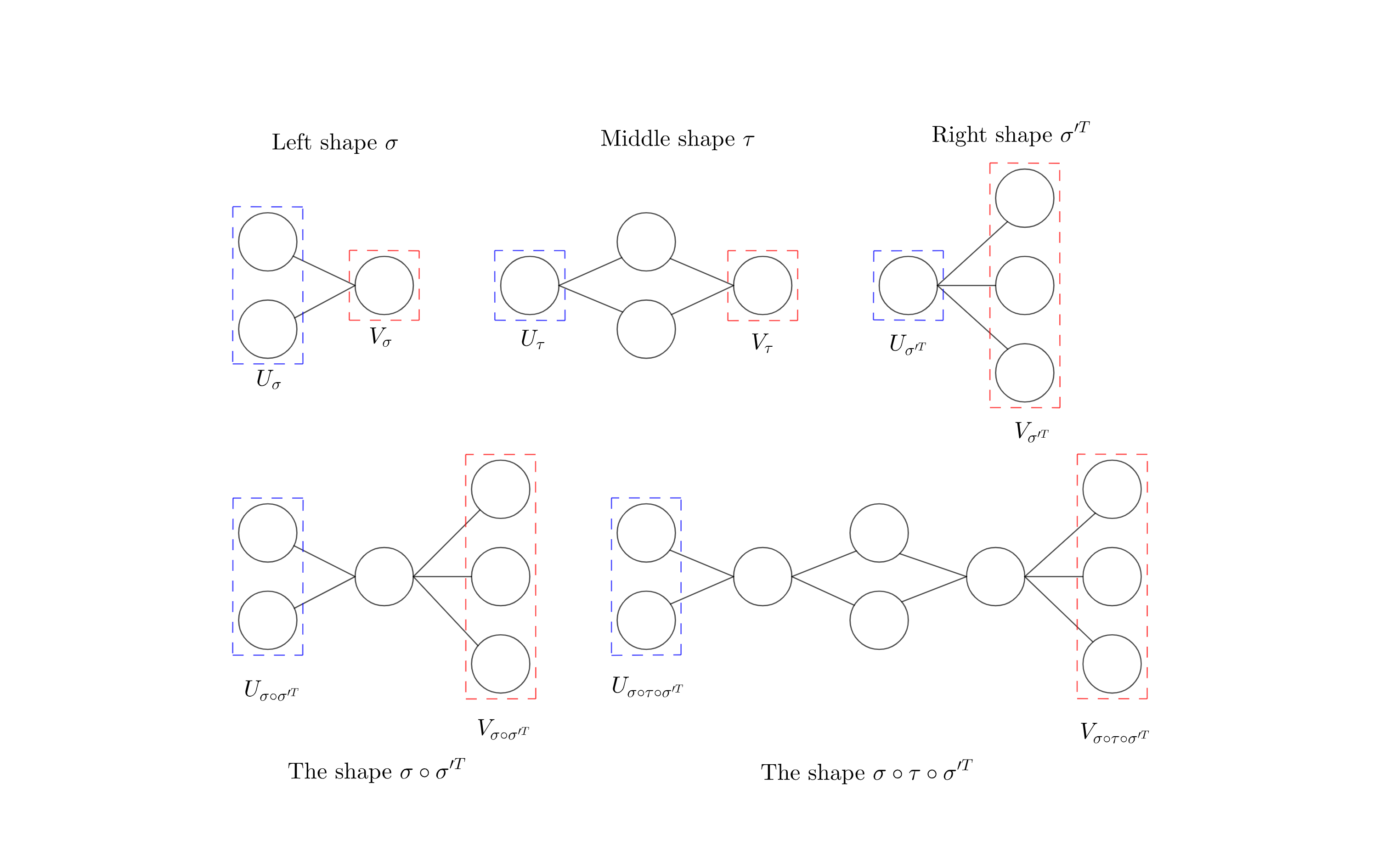
Refer to caption
Figure 4: Illustration of shape composition and decomposition.

Because of the minimality and leftmost/rightmost-ness of the vertex separators S,TS,T used to define σ,τ,σ′\sigma,\tau,\sigma^{\prime}, the shapes σ,τ,σ′\sigma,\tau,\sigma^{\prime} have some special combinatorial structure, which we capture in the following proposition. We defer the proof until Section 7 where we state a generalized version.

Proposition 3.19.

σ\sigma, τ\tau, and σ′T{\sigma^{\prime}}^{T} have the following properties:

  1. 1.

    Vσ=SV_{\sigma}=S is the unique minimum vertex separator of σ\sigma.

  2. 2.

    SS and TT are the leftmost and rightmost minimum vertex separators of τ\tau.

  3. 3.

    T=Uσ′TT=U_{{\sigma^{\prime}}^{T}} is the unique minimum vertex separator of σ′T{\sigma^{\prime}}^{T}.

Based on this, we define sets of shapes which can appear as left, middle, or right parts.

Definition 3.20 (Left, Middle, and Right Parts).

Let α\alpha be a shape.

  1. 1.

    We say that α\alpha is a left part if VαV_{\alpha} is the unique minimum vertex separator of α\alpha, all vertices of α\alpha are reachable from UαU_{\alpha} without passing through VαV_{\alpha}, and E⁡(α)E(\alpha) has no edges which are entirely contained in VαV_{\alpha}.

  2. 2.

    We say that α\alpha is a proper middle part if UαU_{\alpha} is the leftmost minimum vertex separator of α\alpha and VαV_{\alpha} is the rightmost minimum vertex separator of α\alpha

  3. 3.

    We say that α\alpha is a right part if UαU_{\alpha} is the unique minimum vertex separator of α\alpha, all vertices of α\alpha are reachable from VαV_{\alpha} without passing through UαU_{\alpha}, and E⁡(α)E(\alpha) has no edges which are entirely contained in UαU_{\alpha}.

Remark 3.21.

For technical reasons, later on we will need to consider improper middle parts τ\tau where UτU_{\tau} and VτV_{\tau} are not the leftmost and rightmost minimum vertex separators of τ\tau, which is why we make this distinction here.

The following proposition is also straightforward from the definitions.

Proposition 3.22.

A shape σ\sigma is a left part if and only if σT\sigma^{T} is a right part

3.2.2 Products of Graph Matrices

We now analyze what happens when we take the products of graph matrices. Roughly speaking, we will have that if α\alpha can be decomposed into left, middle, and right parts σ\sigma, τ\tau, and σ′T{\sigma^{\prime}}^{T} then Mα≈Mσ​Mτ​Mσ′TM_{\alpha}\approx M_{\sigma}M_{\tau}M_{{\sigma^{\prime}}^{T}}. However, this is only an approximation rather than an equality, and this will be the source of considerable technical difficulties.

We begin with a concatenation operation on ribbons.

Definition 3.23 (Ribbon Concatenation).

If R1R_{1} and R2R_{2} are two ribbons such that V⁡(R1)∩V⁡(R2)=BR1=AR2V(R_{1})\cap V(R_{2})=B_{R_{1}}=A_{R_{2}} and either R1R_{1} or R2R_{2} contains no edges entirely within BR1=AR2B_{R_{1}}=A_{R_{2}} then we define R1∘R2R_{1}\circ R_{2} to be the ribbon formed by glueing together R1R_{1} and R2R_{2} along BR1=AR2B_{R_{1}}=A_{R_{2}}. In other words,

  1. 1.

    V⁡(R1∘R2)=V⁡(R1)∪V⁡(R2)V(R_{1}\circ R_{2})=V(R_{1})\cup V(R_{2})

  2. 2.

    E⁡(R1∘R2)=E⁡(R1)∪E⁡(R2)E(R_{1}\circ R_{2})=E(R_{1})\cup E(R_{2})

  3. 3.

    AR1∘R2=AR1A_{R_{1}\circ R_{2}}=A_{R_{1}} and BR1∘R2=BR2B_{R_{1}\circ R_{2}}=B_{R_{2}}.

The following proposition is easy to check.

Proposition 3.24.

Whenever R1,R2R_{1},R_{2} are ribbons such that R1∘R2R_{1}\circ R_{2} is defined, MR1​MR2=MR1∘R2M_{R_{1}}M_{R_{2}}=M_{R_{1}\circ R_{2}}

We have an analogous definition for concatenating shapes:

Definition 3.25 (Shape Concatenation).

If α1\alpha_{1} and α2\alpha_{2} are two shapes such that V⁡(α1)∩V⁡(α2)=Vα1=Uα2V(\alpha_{1})\cap V(\alpha_{2})=V_{\alpha_{1}}=U_{\alpha_{2}} and either α1\alpha_{1} or α2\alpha_{2} contains no edges entirely within Vα1=Uα2V_{\alpha_{1}}=U_{\alpha_{2}} then we define α1∘α2\alpha_{1}\circ\alpha_{2} to be the shape formed by glueing together α1\alpha_{1} and α2\alpha_{2} along Vα1=Uα2V_{\alpha_{1}}=U_{\alpha_{2}}. In other words,

  1. 1.

    V⁡(α1∘α2)=V⁡(α1)∪V⁡(α2)V(\alpha_{1}\circ\alpha_{2})=V(\alpha_{1})\cup V(\alpha_{2})

  2. 2.

    E⁡(α1∘α2)=E⁡(α1)∪E⁡(α2)E(\alpha_{1}\circ\alpha_{2})=E(\alpha_{1})\cup E(\alpha_{2})

  3. 3.

    Uα1∘α2=Uα1U_{\alpha_{1}\circ\alpha_{2}}=U_{\alpha_{1}} and Vα1∘α2=Vα2V_{\alpha_{1}\circ\alpha_{2}}=V_{\alpha_{2}}.

Example 3.26.

Fig. 4 illustrates an example of shape composition. Observe how the shapes σ∘σ′T\sigma\circ\sigma^{\prime T} and σ∘τ∘σ′T\sigma\circ\tau\circ\sigma^{\prime T} are obtained from the shapes σ,τ\sigma,\tau and σ′T\sigma^{\prime T}.

The next proposition, again easy to check, shows that the shape concatenation operation respects the left/middle/right part decomposition.

Proposition 3.27.

If α\alpha can be decomposed into left, middle, and right parts σ,τ,σ′T\sigma,\tau,{\sigma^{\prime}}^{T} then α=σ∘τ∘σ′T\alpha=\sigma\circ\tau\circ{\sigma^{\prime}}^{T}.

We now discuss why Mα=Mσ∘τ∘σ′T≈Mσ​Mτ​Mσ′TM_{\alpha}=M_{\sigma\circ\tau\circ{\sigma^{\prime}}^{T}}\approx M_{\sigma}M_{\tau}M_{{\sigma^{\prime}}^{T}} is only an approximation rather than an equality. Consider the difference Mσ​Mτ​Mσ′T−Mσ∘τ∘σ′TM_{\sigma}M_{\tau}M_{{\sigma^{\prime}}^{T}}-M_{\sigma\circ\tau\circ{\sigma^{\prime}}^{T}}. The graph matrix Mσ∘τ∘σ′TM_{\sigma\circ\tau\circ{\sigma^{\prime}}^{T}} decomposes (by definition) into a sum over injective maps φ:V⁡(σ∘τ∘σ′T)→[n]\varphi\,:\,V(\sigma\circ\tau\circ{\sigma^{\prime}}^{T})\rightarrow[n]. Also by expanding definitions, the product Mσ​Mτ​Mσ′TM_{\sigma}M_{\tau}M_{{\sigma^{\prime}}^{T}} expands into a sum over triples of injective maps (φ1,φ2,φ3)(\varphi_{1},\varphi_{2},\varphi_{3}), where φ1:V⁡(σ)→[n],φ2:V⁡(τ)→[n],φ3:V⁡(σ′)→[n]\varphi_{1}\,:\,V(\sigma)\rightarrow[n],\varphi_{2}\,:\,V(\tau)\rightarrow[n],\varphi_{3}\,:\,V(\sigma^{\prime})\rightarrow[n] where φ1\varphi_{1} and φ2\varphi_{2} agree on Vσ=UτV_{\sigma}=U_{\tau} and φ2\varphi_{2} and φ3\varphi_{3} agree on Vτ=Uσ′TV_{\tau}=U_{{\sigma^{\prime}}^{T}}.

If they are combined into one map φ:V⁡(σ∪τ∪σ′)→[n]\varphi:V(\sigma\cup\tau\cup{\sigma^{\prime}})\rightarrow[n], the resulting φ\varphi may not be injective because φ1​(V⁡(σ)),φ2​(V⁡(τ)),φ3​(V⁡(σ′T))\varphi_{1}(V(\sigma)),\varphi_{2}(V(\tau)),\varphi_{3}(V({\sigma^{\prime}}^{T})) may have nontrivial intersection (beyond φ1​(Vσ)\varphi_{1}(V_{\sigma}) and φ2​(Vτ)\varphi_{2}(V_{\tau})). We call the resulting terms intersection terms and handling them properly is a major part of the technical analysis.

Remark 3.28.

Actually, the approximation Mα=Mσ∘τ∘σ′T≈Mσ​Mτ​Mσ′TM_{\alpha}=M_{\sigma\circ\tau\circ{\sigma^{\prime}}^{T}}\approx M_{\sigma}M_{\tau}M_{{\sigma^{\prime}}^{T}} is also off by a multiplicative constant because there is also a subtle issue involving the automorphism groups of these shapes. For now, we ignore this issue. For details about this issue, see Lemma 7.82.

3.3 Shape Coefficient Matrices

The idea for our analysis is as follows. Given a matrix-valued function Λ\Lambda which is symmetric under permutations of [n][n], we write Λ=∑αλα​Mα\Lambda=\sum_{\alpha}{\lambda_{\alpha}M_{\alpha}}. We then break each shape α\alpha up into left, middle, and right parts σ\sigma, τ\tau, and σ′T{\sigma^{\prime}}^{T}.

For this analysis, we use shape coefficient matrices HτH_{\tau} whose rows and columns are indexed by left shapes and whose entries depend on the coefficients λα\lambda_{\alpha}. We choose these matrices so that

Λ=∑τHτ​(σ,σ′)​Mσ∘τ∘σ′T≈∑τHτ​(σ,σ′)​Mσ​Mτ​Mσ′T\Lambda=\sum_{\tau}{H_{\tau}(\sigma,\sigma^{\prime})M_{\sigma\circ\tau\circ{\sigma^{\prime}}^{T}}}\approx\sum_{\tau}{H_{\tau}(\sigma,\sigma^{\prime})M_{\sigma}M_{\tau}M_{{\sigma^{\prime}}^{T}}}

To set this up, we separate the possible middle parts τ\tau into groups based on the size of UτU_{\tau} and whether or not they are trivial.

Definition 3.29.

We define ℐm​i​d\mathcal{I}_{mid} to be the set of all possible UτU_{\tau}. Here ℐm​i​d\mathcal{I}_{mid} is the set of tuples of unspecified vertices of the form U=(u1,…,uk)U=(u_{1},\ldots,u_{k}) where 0≤k≤d0\leq k\leq d.

Definition 3.30.

We say that a proper middle shape τ\tau is trivial if E⁡(τ)=∅E(\tau)=\emptyset and |Uτ∩Vτ|=|Uτ|=|Vτ||U_{\tau}\cap V_{\tau}|=|U_{\tau}|=|V_{\tau}| (i.e. VτV_{\tau} is a permutation of UτU_{\tau}).

For simplicity, the only proper trivial middle parts τ\tau we consider are shapes I​dUId_{U} corresponding to identity matrices.

Definition 3.31.

Given a tuple of unspecified vertices U=(u1,…,u|U|)U=(u_{1},\ldots,u_{|U|}) We define I​dUId_{U} to be the shape where V⁡(I​dU)=UV(Id_{U})=U, UI​dU=VI​dU=UU_{Id_{U}}=V_{Id_{U}}=U, and E⁡(I​dU)=∅E(Id_{U})=\emptyset.

We group all of the proper non-trivial middle parts τ\tau into sets ℳU\mathcal{M}_{U} based on the size of UτU_{\tau}.

Definition 3.32.

Given a tuple of unspecified vertices U=(u1,…,u|U|)U=(u_{1},\ldots,u_{|U|}), we define ℳU\mathcal{M}_{U} to be the set of proper non-trivial middle parts τ\tau such that UτU_{\tau} and VτV_{\tau} have the same size as UU. Note that UτU_{\tau} and VτV_{\tau} may intersect each other arbitrarily.

With these definitions, we can now define our shape coefficient matrices.

Definition 3.33.

Given U∈ℐm​i​dU\in\mathcal{I}_{mid}, we define ℒU\mathcal{L}_{U} to be the set of left shapes σ\sigma such that |Vσ|=|U||V_{\sigma}|=|U|.

Definition 3.34.

For each U∈ℐm​i​dU\in\mathcal{I}_{mid}, we define the shape coefficient matrix HI​dUH_{Id_{U}} to be the matrix indexed by left shapes σ,σ′∈ℒU\sigma,\sigma^{\prime}\in\mathcal{L}_{U} with entries HI​dU​(σ,σ′)=1|U|!​λσ∘σ′TH_{Id_{U}}(\sigma,\sigma^{\prime})=\frac{1}{|U|!}\lambda_{\sigma\circ{\sigma^{\prime}}^{T}}

Definition 3.35.

For each U∈ℐm​i​dU\in\mathcal{I}_{mid}, for each τ∈ℳU\tau\in\mathcal{M}_{U}, we define the shape coefficient matrix HτH_{\tau} to be the matrix indexed by left shapes σ,σ′∈ℒU\sigma,\sigma^{\prime}\in\mathcal{L}_{U} with entries Hτ​(σ,σ′)=1(|U|!)2​λσ∘τ∘σ′TH_{\tau}(\sigma,\sigma^{\prime})=\frac{1}{(|U|!)^{2}}\lambda_{\sigma\circ\tau\circ{\sigma^{\prime}}^{T}}

With these shape coefficient matrices, we have the following decomposition of Λ=∑αλα​Mα\Lambda=\sum_{\alpha}{\lambda_{\alpha}M_{\alpha}}.

Lemma 3.36.

Λ=∑U∈ℐm​i​d∑σ,σ′∈ℒUHI​dU​(σ,σ′)​Mσ∘σ′T+∑U∈ℐm​i​d∑τ∈ℳU∑σ,σ′∈ℒUHτ​(σ,σ′)​Mσ∘τ∘σ′T\Lambda=\sum_{U\in\mathcal{I}_{mid}}{\sum_{\sigma,\sigma^{\prime}\in\mathcal{L}_{U}}{H_{Id_{U}}(\sigma,\sigma^{\prime})M_{\sigma\circ{\sigma^{\prime}}^{T}}}}+\sum_{U\in\mathcal{I}_{mid}}{\sum_{\tau\in\mathcal{M}_{U}}{\sum_{\sigma,\sigma^{\prime}\in\mathcal{L}_{U}}{H_{\tau}(\sigma,\sigma^{\prime})M_{\sigma\circ\tau\circ{\sigma^{\prime}}^{T}}}}}

We defer the proof of this lemma to Lemma 7.85.

For technical reasons, we need to define one more operation to handle intersection terms. We call this operation the −γ,γ-\gamma,\gamma operation.

Definition 3.37.

Given U,V∈ℐm​i​dU,V\in\mathcal{I}_{mid} where |U|>|V||U|>|V|, we define ΓU,V\Gamma_{U,V} to be the set of left parts γ\gamma such that |Uγ|=|U||U_{\gamma}|=|U| and |Vγ|=|V||V_{\gamma}|=|V|.

Definition 3.38.

Given U,V∈ℐm​i​dU,V\in\mathcal{I}_{mid} where |U|>|V||U|>|V|, a shape coefficient matrix HI​dVH_{Id_{V}}, and a γ∈ΓU,V\gamma\in\Gamma_{U,V}, we define the shape coefficient matrix HI​dV−γ,γH^{-\gamma,\gamma}_{Id_{V}} to be the matrix indexed by left shapes σ,σ′∈ℒU\sigma,\sigma^{\prime}\in\mathcal{L}_{U} with entries HI​dV−γ,γ​(σ,σ′)=H⁡(σ∘γ,σ′∘γ)H^{-\gamma,\gamma}_{Id_{V}}(\sigma,\sigma^{\prime})=H(\sigma\circ\gamma,\sigma^{\prime}\circ\gamma)

3.4 Informal Theorem Statement

We are now ready to state a simplified, qualitative version of our main theorem. For the full, quantitative version of our main theorem, see Theorem 7.102.

Theorem 3.39.

There exist functions f⁡(τ):ℳU→ℝf(\tau):\mathcal{M}_{U}\rightarrow{\mathbb{R}} and f⁡(γ):ΓU,V→ℝf(\gamma):\Gamma_{U,V}\rightarrow{\mathbb{R}} depending on nn and other parameters such that if Λ=∑αλα​Mα\Lambda=\sum_{\alpha}{\lambda_{\alpha}M_{\alpha}} and the following conditions hold:

  1. 1.

    (PSD mass) For all U∈ℐm​i​dU\in\mathcal{I}_{mid}, HI​dU⪰0H_{Id_{U}}\succeq 0

  2. 2.

    (Middle shape bounds) For all U∈ℐm​i​dU\in\mathcal{I}_{mid} and all τ∈ℳU\tau\in\mathcal{M}_{U},

    [HI​dUf⁡(τ)​Hτf⁡(τ)​HτTHI​dU]⪰0\left[{\begin{array}[]{cc}H_{Id_{U}}&f(\tau)H_{\tau}\\ f(\tau)H^{T}_{\tau}&H_{Id_{U}}\end{array}}\right]\succeq 0
  3. 3.

    (Intersection term bounds) For all U,V∈ℐm​i​dU,V\in\mathcal{I}_{mid} such that |U|>|V||U|>|V| and all γ∈ΓU,V\gamma\in\Gamma_{U,V}, HI​dVγ−γ,γ⪯f⁡(γ)​HI​dUγH^{-\gamma,\gamma}_{Id_{V_{\gamma}}}\preceq f(\gamma)H_{Id_{U_{\gamma}}}

then with probability at least 1−o⁡(1)1-o(1) over G∼{±1}(n2)G\sim\{\pm 1\}^{n\choose 2} it holds that Λ⁡(G)⪰0\Lambda(G)\succeq 0.

Remark 3.40.

Condition 11 of Theorem 3.39 will follow from condition 22 but we state it explicitly since it will correspond to the dominating terms of the approximate PSD decomposition. And in applications, it will be both easy to verify and will shed light on the structure of the coefficients which in turn will be useful for verifying conditions 22 and 33.

Remark 3.41.

As we will demonstrate in the remainder of this paper, our machinery works well when the coefficients λα\lambda_{\alpha} has some decay for each vertex or edge in the shape. In many settings, this can be done quite easily by adding noise to the distribution, such as resampling part of the input, or by lowering the parameters slightly, such as m≤nk/4−εm\leq n^{k/4-\varepsilon} instead of m≤nk/4m\leq n^{k/4}.

3.4.1 Choice of functions f⁡(τ)f(\tau) and f⁡(γ)f(\gamma)

In a rough sense, f⁡(τ)f(\tau) measures the blow-up in the norm by using MτM_{\tau} instead of MI​dUM_{Id_{U}} in the corresponding term of the Fourier decomposition. So we choose f⁡(τ)f(\tau) to be ‖Mτ‖\left\lVert M_{\tau}\right\rVert, upto lower order terms. Our second condition verifies that the coefficients that arise because of this τ\tau (which are encoded in HτH_{\tau}) are sufficiently small to overpower this norm blowup.

The fact that ‖Mτ‖\left\lVert M_{\tau}\right\rVert is equal to O~​(n|V⁡(τ)|−|Uτ|2)\tilde{O}(n^{\frac{|V(\tau)|-|U_{\tau}|}{2}}) has been shown in previous works [BHK+16, AMP20]. So, we choose f⁡(τ)f(\tau) to be O~​(n|V⁡(τ)|−|Uτ|2)\tilde{O}(n^{\frac{|V(\tau)|-|U_{\tau}|}{2}}) where the problem instance is on Gn,1/2G_{n,1/2}. For problems with Gaussian or other inputs, similar forms of f⁡(τ)f(\tau) can be used, which have been shown formally in the work of [AMP20]. When we state the main theorem in general, we use a single f⁡(τ)f(\tau) that incorporates all of these settings.

f⁡(γ)f(\gamma) is a bit trickier to describe. In our analysis, we roughly collect intersection terms from the approximate PSD decomposition and charge them to shapes of the form σ∘γ∘γT∘σ′T\sigma\circ\gamma\circ\gamma^{T}\circ\sigma^{\prime T}. Using the same idea as the previous step, we charge these to shapes with trivial middle shapes. Roughly, f⁡(γ)f(\gamma) for a fixed γ\gamma upper bounds the blowup from the norms of the original shape as compared to the new intersection shape. The third condition argues that the the original coefficients are sufficiently small to compensate for these blowups.

For problems on Gn,1/2G_{n,1/2}, we set f⁡(γ)=O~​(n|V⁡(γ)∖Uγ|)f(\gamma)=\tilde{O}(n^{|V(\gamma)\setminus U_{\gamma}|}). For problems with Gaussian inputs, we choose essentially the same function, but they fall under the umbrella of generalized graph matrices, where V⁡(γ)V(\gamma) and UγU_{\gamma} are defined accordingly. Indeed, in our main theorem, we encompass both these settings with a single choice of f⁡(γ)f(\gamma).

3.5 An informal application to planted clique

Before we move on to further definitions needed for a more complete statement of the main theorem, we present an informal example.

Example 3.42.

When the pseudo-calibration method is applied to prove an SoS lower bound for the planted clique problem in nn node graphs with clique size kk, as in [BHK+16], the matrix-valued function which results is Λ=∑α:|V⁡(α)|≤t(kn)|V⁡(α)|Mα\Lambda=\sum_{\alpha\,:\,|V(\alpha)|\leq t}{\left(\frac{k}{n}\right)^{|V(\alpha)|}M_{\alpha}} where t≈log⁡(n)t\approx\log(n). One may then compute that the matrices HI​dUH_{Id_{U}} and HτH_{\tau} are as follows (at least so long as |V⁡(σ)|,|V⁡(τ)|,|V⁡(σ′)|≪t|V(\sigma)|,|V(\tau)|,|V(\sigma^{\prime})|\ll t; we ignore this detail for now). For all r∈[0,d2]r\in[0,\frac{d}{2}],

  1. 1.

    For UU with |U|=r|U|=r, HI​dU​(σ,σ′)=(kn)|V⁡(σ)|+|V⁡(σ′)|−rH_{Id_{U}}(\sigma,\sigma^{\prime})=\left(\frac{k}{n}\right)^{|V(\sigma)|+|V(\sigma^{\prime})|-r}

  2. 2.

    For all proper, non-trivial middle shapes τ\tau such that |Uτ|=|Vτ|=r|U_{\tau}|=|V_{\tau}|=r,

    Hτ​(σ,σ′)=(kn)|V⁡(σ)|+|V⁡(σ′)|+|V⁡(τ)|−2​rH_{\tau}(\sigma,\sigma^{\prime})=\left(\frac{k}{n}\right)^{|V(\sigma)|+|V(\sigma^{\prime})|+|V(\tau)|-2r}

Defining vrv_{r} to be the vector such that vr​(σ)=(kn)|V⁡(σ)|−r2v_{r}(\sigma)=\left(\frac{k}{n}\right)^{|V(\sigma)|-\frac{r}{2}}, we have that

  1. 1.

    For UU with |U|=r|U|=r, HI​dU=v|U|​v|U|TH_{Id_{U}}={v_{|U|}}{v^{T}_{|U|}}

  2. 2.

    For all proper, non-trivial middle shapes τ\tau such that |Uτ|=|Vτ|=r|U_{\tau}|=|V_{\tau}|=r, Hτ=(kn)|V⁡(τ)|−r​vr​vrTH_{\tau}=\left(\frac{k}{n}\right)^{|V(\tau)|-r}{v_{r}}{v^{T}_{r}}

  3. 3.

    For all left parts γ\gamma, HI​dVγ−γ,γ=(kn)2​|V⁡(γ)|−|Uγ|−|Vγ|​v|Uγ|​v|Uγ|TH^{-\gamma,\gamma}_{Id_{V_{\gamma}}}=\left(\frac{k}{n}\right)^{2|V(\gamma)|-|U_{\gamma}|-|V_{\gamma}|}v_{|U_{\gamma}|}v^{T}_{|U_{\gamma}|}

It turns out in this setting that we can take f⁡(τ)f(\tau) to be O~​(n|V⁡(τ)|−|Uτ|2)\tilde{O}(n^{\frac{|V(\tau)|-|U_{\tau}|}{2}}) and f⁡(γ)f(\gamma) to be O~​(n|V⁡(γ)∖Uγ|)\tilde{O}(n^{|V(\gamma)\setminus U_{\gamma}|}). Thus, as long as k≪nk\ll\sqrt{n},

  1. 1.

    For any UU and all τ\tau such that Vτ≠UτV_{\tau}\neq U_{\tau} with |Uτ|=|Vτ|=|U||U_{\tau}|=|V_{\tau}|=|U|, f⁡(τ)​Hτ⪯HI​dUf(\tau)H_{\tau}\preceq H_{Id_{U}}.

  2. 2.

    For all non-trivial left parts γ\gamma, HI​dVγ−γ,γ⪯f⁡(γ)​HI​dUγH^{-\gamma,\gamma}_{Id_{V_{\gamma}}}\preceq f(\gamma)H_{Id_{U_{\gamma}}}

Remark 3.43.

This does not quite satisfy the conditions of Theorem 3.39 because there are τ\tau such that Vτ=UτV_{\tau}=U_{\tau} but which are non-trivial because E⁡(τ)≠∅E(\tau)\neq\emptyset. For these τ\tau, condition 2 of Theorem 3.39 fails. In order to prove their SoS lower bounds for planted clique, [BHK+16] handle this issue by grouping together all of the τ\tau where Vτ=UτV_{\tau}=U_{\tau} into the indicator function for whether Vτ=UτV_{\tau}=U_{\tau} is a clique.

Since this issue is specific to planted clique, we don’t try to incorporate it into the machinery to avoid losing generality.

For the sake of exposition, a detailed analysis with figures of all the shapes and all the coefficient matrices that appear for the degree-44 SoS lower bound for planted clique is given in Appendix C. Note that we present these details purely for the interested reader and they are not needed to apply the machinery.

3.6 Generalizing the machinery

In this section, we restricted ourselves to the case when the input is from {−1,1}(n2)\{-1,1\}^{\binom{n}{2}} for simplicity. However, for our results we will need to handle more general types of inputs. We now briefly describe which kinds of inputs we will need to handle and how we handle them.

  1. 1.

    In general, the entries of the input may be labeled by more than 22 indices. For example, for tensor PCA on order 33 tensors, the entries of the input are indexed by 33 indices. To handle this, we will have shapes which have hyperedges rather than edges.

  2. 2.

    In general, the entries of the input will come from a distribution Ω\Omega rather than being ±1\pm{1}. To handle this, we will take an orthonormal basis {hk}\{h_{k}\} for Ω\Omega. We will then give each edge/hyperedge a label ll to specify which polynomial hlh_{l} should be applied to that entry of the input.

  3. 3.

    In general, there may be tt different types of indices rather than just one type of index. In this case, the symmetry group will be Sn1×…×SntS_{n_{1}}\times\ldots\times S_{n_{t}} rather than SnS_{n}. To handle this, we will have shapes with different types of vertices.

We formally make these generalizations in Section 7.

3.7 Further definitions needed for our applications

We will describe some more notations and definitions that will be useful to us to describe the qualitative bounds for our applications. For each of our applications, we will describe the corresponding modifications needed to the definitions already in place and present new definitions where necessary.

3.7.1 Planted slightly denser subgraph

Since the input is a graph G∈{−1,1}([n]2)G\in\{-1,1\}^{\binom{[n]}{2}}, most of what we introduced already apply to this setting. To describe the moment matrix, we need to define the truncation parameter.

Definition 3.44 (Truncation parameters).

For integers Ds​o​s,DV≥0D_{sos},D_{V}\geq 0, say that a shape α\alpha satisfies the truncation parameters Ds​o​s,DVD_{sos},D_{V} if

  • -

    The degrees of the monomials that UαU_{\alpha} and VαV_{\alpha} correspond to, are at most Ds​o​s2\frac{D_{sos}}{2}

  • -

    The left part σ\sigma, the middle part τ\tau and the right part σ′\sigma^{\prime} of α\alpha satisfy |V⁡(σ)|,|V⁡(τ)|,|V⁡(σ′)|≤DV|V(\sigma)|,|V(\tau)|,|V(\sigma^{\prime})|\leq D_{V}

3.7.2 Tensor PCA

We consider the input to be a tensor A∈ℝ[n]kA\in\mathbb{R}^{[n]^{k}}. The input entries are now sampled from the distribution 𝒩⁡(0,1)\mathcal{N}(0,1) instead of {−1,1}\{-1,1\}. So, we will work with the Hermite basis of polynomials. Let the standard unnormalized Hermite polynomials be denoted as h0(x)=1,h1(x)=x,h2(x)=x2−1,…h_{0}(x)=1,h_{1}(x)=x,h_{2}(x)=x^{2}-1,\ldots. Then, we work with the basis ha​(A):=∏e∈[n]khe​(Ae)h_{a}(A):=\prod_{e\in[n]^{k}}h_{e}(A_{e}) over a∈ℕ[n]ka\in\mathbb{N}^{[n]^{k}}. Accordingly, we will modify the graphs that represent ribbons (and by extension, shapes), to have labeled hyperedges of arity kk. So, an hyperedge ee with a label tt will correspond to the hermite polynomial ht​(Ae)h_{t}(A_{e}).

Definition 3.45 (Hyperedges).

Instead of standard edges, we will have labeled hyperedges of arity kk in the underlying graphs for our ribbons as well as shapes. The label for an hyperedge ee, denoted lel_{e}, is an element of ℕ\mathbb{N} which will correspond to the Hermite polynomial being evaluated on that entry.

Note that our hyperedges are ordered since the tensor AA is not necessarily symmetric.

For variables x1,…,xnx_{1},\ldots,x_{n}, the rows and columns of our moment matrix will now correspond to monomials of the form ∏i≤nxipi\prod_{i\leq n}x_{i}^{p_{i}} for pi≥0p_{i}\geq 0. To capture this, we use the notion of index shape pieces and index shapes. Informally, we split the above monomial product into groups based on their powers and each such group will form an index shape piece.

Definition 3.46 (Index shape piece).

An index shape piece Ui=((Ui,1,…,Ui,t),pi)U_{i}=((U_{i,1},\ldots,U_{i,t}),p_{i}) is a tuple of indices (Ui,1,…,Ui,t)(U_{i,1},\ldots,U_{i,t}) along with a power pi∈ℕp_{i}\in\mathbb{N}. Let V⁡(Ui)V(U_{i}) be the set {Ui,1,…,Ui,t}\{U_{i,1},\ldots,U_{i,t}\} of vertices of this index shape piece. When clear from context, we use UiU_{i} instead of V⁡(Ui)V(U_{i}).

If we realize Ui,1,…,Ui,tU_{i,1},\ldots,U_{i,t} to be indices a1,…,at∈[n]a_{1},\ldots,a_{t}\in[n], then, this realization of this index shape piece corresponds to the monomial ∏j≤txajpi\prod_{j\leq t}x_{a_{j}}^{p_{i}}.

Definition 3.47 (Index shape).

An index shape UU is a set of index shape pieces UiU_{i} that have different powers. Let V⁡(U)V(U) be the set of vertices ∪iV(Ui)\cup_{i}V(U_{i}). When clear from context, we use UU instead of V⁡(U)V(U).

Observe that each realization of an index shape corresponds to a row or column of the moment matrix.

Definition 3.48.

For two index shapes U,VU,V, we write U≡VU\equiv V if for all powers pp, the index shape pieces of power pp in UU and VV have the same length.

Definition 3.49.

Define ℐm​i​d{\mathcal{I}}_{mid} to be the set of all index shapes UU that contain only index shape pieces of power 11.

In the definition of shapes, the distinguished set of vertices should now be replaced by index shapes.

Definition 3.50 (Shapes).

Shapes are tuples α=(Hα,Uα,Vα)\alpha=(H_{\alpha},U_{\alpha},V_{\alpha}) where HαH_{\alpha} is a graph with hyperedges of arity kk and Uα,VαU_{\alpha},V_{\alpha} are index shapes such that Uα,Vα⊆V⁡(Hα)U_{\alpha},V_{\alpha}\subseteq V(H_{\alpha}).

Definition 3.51 (Proper shape).

A shape α\alpha is proper if it has no isolated vertices outside Uα∪VαU_{\alpha}\cup V_{\alpha}, no multi-edges and all the edges have a nonzero label.

To define the notion of vertex separators, we modify the notion of paths for hyperedges.

Definition 3.52 (Path).

A path is a sequence of vertices u1,…,utu_{1},\ldots,u_{t} such that ui,ui+1u_{i},u_{i+1} are in the same hyperedge, for all i≤t−1i\leq t-1.

The notions of vertex separator and decomposition into left, middle and right parts are identically defined with the above notion of hyperedges and paths. In Section 7, we will show that they are well defined.

In the definition of trivial shape τ\tau, we now require Uτ≡VτU_{\tau}\equiv V_{\tau}. For U∈ℐm​i​dU\in{\mathcal{I}}_{mid}, ℳU{\mathcal{M}}_{U} will be the set of proper non-trivial middle parts τ\tau with Uτ≡Vτ≡UU_{\tau}\equiv V_{\tau}\equiv U and ℒU{\mathcal{L}}_{U} will be the set of left parts σ\sigma such that Vσ≡UV_{\sigma}\equiv U. Similarly, for U,V∈ℐm​i​dU,V\in{\mathcal{I}}_{mid}, ℒU,V{\mathcal{L}}_{U,V} will be the set of left parts γ\gamma such that Uγ≡UU_{\gamma}\equiv U and Vγ≡VV_{\gamma}\equiv V.

In order to define the moment matrix, we need to truncate our shapes based on the number of vertices and the labels on our hyperedges. So, we make the following definition.

Definition 3.53 (Truncation parameters).

For integers Ds​o​s,DV,DE≥0D_{sos},D_{V},D_{E}\geq 0, say that a shape α\alpha satisfies the truncation parameters Ds​o​s,DV,DED_{sos},D_{V},D_{E} if

  • -

    The degrees of the monomials that UαU_{\alpha} and VαV_{\alpha} correspond to, are at most Ds​o​s2\frac{D_{sos}}{2}

  • -

    The left part σ\sigma, the middle part τ\tau and the right part σ′T\sigma^{\prime T} of α\alpha satisfy |V⁡(σ)|,|V⁡(τ)|,|V⁡(σ′T)|≤DV|V(\sigma)|,|V(\tau)|,|V(\sigma^{\prime T})|\leq D_{V}

  • -

    For each e∈E⁡(α)e\in E(\alpha), le≤DEl_{e}\leq D_{E}.

3.7.3 Sparse PCA

We consider the mm vectors v1,…,vm∈ℝdv_{1},\ldots,v_{m}\in\mathbb{R}^{d} to be the input. Similar to Tensor PCA, we will work with the Hermite basis of polynomials since the entries are sampled from the distribution 𝒩⁡(0,1)\mathcal{N}(0,1). In particular, if we denote the unnormalized Hermite polynomials by h0(x)=1,h1(x)=x,h2(x)=x2−1,…h_{0}(x)=1,h_{1}(x)=x,h_{2}(x)=x^{2}-1,\ldots, then, we work with the basis ha​(v):=∏i∈[m],j∈[n]hai,j​(vi,j)h_{a}(v):=\prod_{i\in[m],j\in[n]}h_{a_{i,j}}(v_{i,j}) over a∈ℕm×na\in\mathbb{N}^{m\times n}. To capture this basis, we will modify the graphs that represent ribbons (and by extension, shapes), to be bipartite graphs with two types of vertices, and have labeled edges that go across vertices of different types. So, an edge (i,j)(i,j) with label tt between a vertex ii of type 11 and a vertex jj of type 22 will correspond to ht​(vi,j)h_{t}(v_{i,j}).

Definition 3.54 (Vertices).

We will have two types of vertices, the vertices corresponding to the mm input vectors that we call type 11 vertices and the vertices corresponding to ambient dimension of the space that we call type 22 vertices.

Definition 3.55 (Edges).

Edges will go across vertices of different types, thereby forming a bipartite graph. An edge between a type 11 vertex ii and a type 2 vertex jj corresonds to the input entry vi,jv_{i,j}. Each edge will have a label in ℕ\mathbb{N} corresponding to the Hermite polynomial evaluated on that entry.

We will have variables x1,…,xnx_{1},\ldots,x_{n} in our SoS program, so we will work with index shape pieces and index shapes as in Tensor PCA, since the rows and columns of our moment matrix will now correspond to monomials of the form ∏i≤nxipi\prod_{i\leq n}x_{i}^{p_{i}} for pi≥0p_{i}\geq 0. But since in our decompositions into left, right and middle parts, we will have type 22 vertices as well in the vertex separators, we will define a generalized notion of index shape pieces and index shapes.

Definition 3.56 (Index shape piece).

An index shape piece Ui=((Ui,1,…,Ui,t),ti,pi)U_{i}=((U_{i,1},\ldots,U_{i,t}),t_{i},p_{i}) is a tuple of indices (Ui,1,…,Ui,t)(U_{i,1},\ldots,U_{i,t}) along a type ti∈{1,2}t_{i}\in\{1,2\} with a power pi∈ℕp_{i}\in\mathbb{N}. Let V⁡(Ui)V(U_{i}) be the set {Ui,1,…,Ui,t}\{U_{i,1},\ldots,U_{i,t}\} of vertices of this index shape piece. When clear from context, we use UiU_{i} instead of V⁡(Ui)V(U_{i}).

For an index shape piece ((Ui,1,…,Ui,t),ti,pi)((U_{i,1},\ldots,U_{i,t}),t_{i},p_{i}) with type ti=2t_{i}=2, if we realize Ui1,…,UitU_{i_{1}},\ldots,U_{i_{t}} to be indices a1,…,at∈[n]a_{1},\ldots,a_{t}\in[n], then, this index shape pieces correspond this to the monomial ∏j≤nxajpi\prod_{j\leq n}x_{a_{j}}^{p_{i}}.

Definition 3.57 (Index shape).

An index shape UU is a set of index shape pieces UiU_{i} that have either have different types or different powers. Let V⁡(U)V(U) be the set of vertices ∪iV(Ui)\cup_{i}V(U_{i}). When clear from context, we use UU instead of V⁡(U)V(U).

Observe that each realization of an index shape corresponds to a row or column of the moment matrix. For our moment matrix, the only nonzero rows correspond to index shapes that have only index shape pieces of type 22, since the only SoS variables are x1​…,xnx_{1}\ldots,x_{n}, but in order to do our analysis, we need to work with the generalized notion of index shapes that allow index shape pieces of both types.

Definition 3.58.

For two index shapes U,VU,V, we write U≡VU\equiv V if for all types tt and all powers pp, the index shape pieces of type tt and power pp in UU and VV have the same length.

Definition 3.59.

Define ℐm​i​d{\mathcal{I}}_{mid} to be the set of all index shapes UU that contain only index shape pieces of power 11.

Since we are working with standard graphs, the notion of path and vertex separator need no modifications, but we will now use the minimum weight vertex separator instead of the minimum vertex separator where we define the weight as follows.

Definition 3.60 (Weight of an index shape).

Suppose we have an index shape U={U1,U2}∈ℐm​i​dU=\{U_{1},U_{2}\}\in{\mathcal{I}}_{mid} where U1=((U1,1,…,U1,|U1|),1,1)U_{1}=((U_{1,1},\ldots,U_{1,|U_{1}|}),1,1) is an index shape piece of type 11 and U2=((U2,1,…,U2,|U2|),2,1)U_{2}=((U_{2,1},\ldots,U_{2,|U_{2}|}),2,1) is an index shape piece of type 22. Then, define the weight of this index shape to be w⁡(U)=m|U1|​n|U2|w(U)=\sqrt{m}^{|U_{1}|}\sqrt{n}^{|U_{2}|}.

We now give the modified definition of shapes.

Definition 3.61 (Shapes).

Shapes are tuples α=(Hα,Uα,Vα)\alpha=(H_{\alpha},U_{\alpha},V_{\alpha}) where HαH_{\alpha} is a graph with two types of vertices, has labeled edges only across vertices of different types and Uα,VαU_{\alpha},V_{\alpha} are index shapes such that Uα,Vα⊆V⁡(Hα)U_{\alpha},V_{\alpha}\subseteq V(H_{\alpha}).

Definition 3.62 (Proper shape).

A shape α\alpha is proper if it has no isolated vertices outside Uα∪VαU_{\alpha}\cup V_{\alpha}, no multi-edges and all the edges have a nonzero label.

In Section 7, we will show that with this new definition of weight and shapes, any shape α\alpha has a unique decomposition into σ∘τ∘σ′T\sigma\circ\tau\circ\sigma^{\prime T} where σ,τ,σ′T\sigma,\tau,\sigma^{\prime T} are left, middle and right parts respectively. Here, τ\tau may possibly be improper.

In the definition of trivial shape τ\tau, we now require Uτ≡VτU_{\tau}\equiv V_{\tau}. For U∈ℐm​i​dU\in{\mathcal{I}}_{mid}, ℳU{\mathcal{M}}_{U} will be the set of proper non-trivial middle parts τ\tau with Uτ≡Vτ≡UU_{\tau}\equiv V_{\tau}\equiv U and ℒU{\mathcal{L}}_{U} will be the set of left parts σ\sigma such that Vσ≡UV_{\sigma}\equiv U. Similarly, for U,V∈ℐm​i​dU,V\in{\mathcal{I}}_{mid}, ℒU,V{\mathcal{L}}_{U,V} will be the set of left parts γ\gamma such that Uγ≡UU_{\gamma}\equiv U and Vγ≡VV_{\gamma}\equiv V.

Finally, in order to define the moment matrix, we need to truncate our shapes based on the number of vertices and the labels on our edges. So, we make the following definition.

Definition 3.63 (Truncation parameters).

For integers Ds​o​s,DV,DE≥0D_{sos},D_{V},D_{E}\geq 0, say that a shape α\alpha satisfies the truncation parameters Ds​o​s,DV,DED_{sos},D_{V},D_{E} if

  • -

    The degrees of the monomials that UαU_{\alpha} and VαV_{\alpha} correspond to, are at most Ds​o​s2\frac{D_{sos}}{2}

  • -

    The left part σ\sigma, the middle part τ\tau and the right part σ′T\sigma^{\prime T} of α\alpha satisfy |V⁡(σ)|,|V⁡(τ)|,|V⁡(σ′T)|≤DV|V(\sigma)|,|V(\tau)|,|V(\sigma^{\prime T})|\leq D_{V}

  • -

    For each e∈E⁡(α)e\in E(\alpha), le≤DEl_{e}\leq D_{E}.

3.7.4 Relaxing the third condition

In Theorem 3.39, the third qualitative condition we’d like to show is as follows: For all U,V∈ℐm​i​dU,V\in\mathcal{I}_{mid} such that |U|>|V||U|>|V| and all γ∈ΓU,V\gamma\in\Gamma_{U,V}, HI​dVγ−γ,γ⪯f⁡(γ)​HI​dUγH^{-\gamma,\gamma}_{Id_{V_{\gamma}}}\preceq f(\gamma)H_{Id_{U_{\gamma}}}. For technical reasons, we won’t be able to show this directly. To handle this, we instead work with a slight modification of HI​dUγH_{Id_{U_{\gamma}}}, a matrix Hγ′H_{\gamma}^{\prime} that’s very close to HI​dUγH_{Id_{U_{\gamma}}}. So, what we will end up showing is: For all U,V∈ℐm​i​dU,V\in\mathcal{I}_{mid} such that |U|>|V||U|>|V| and all γ∈ΓU,V\gamma\in\Gamma_{U,V}, HI​dVγ−γ,γ⪯f⁡(γ)​Hγ′H^{-\gamma,\gamma}_{Id_{V_{\gamma}}}\preceq f(\gamma)H^{\prime}_{\gamma}.

Let DVD_{V} be the truncation parameter. A canonical choice for Hγ′H^{\prime}_{\gamma} is to take

  1. 1.

    Hγ′​(σ,σ′)=HI​dU​(σ,σ′)H^{\prime}_{\gamma}(\sigma,\sigma^{\prime})=H_{Id_{U}}(\sigma,\sigma^{\prime}) whenever |V⁡(σ∘γ)|≤DV|V(\sigma\circ\gamma)|\leq D_{V} and |V⁡(σ′∘γ)|≤DV|V(\sigma^{\prime}\circ\gamma)|\leq D_{V}.

  2. 2.

    Hγ′​(σ,σ′)=0H^{\prime}_{\gamma}(\sigma,\sigma^{\prime})=0 whenever |V⁡(σ∘γ)|>DV|V(\sigma\circ\gamma)|>D_{V} or |V⁡(σ′∘γ)|>DV|V(\sigma^{\prime}\circ\gamma)|>D_{V}.

With this choice, Hγ′H_{\gamma}^{\prime} is the same as HI​dUγH_{Id_{U_{\gamma}}} upto truncation error. We will formally bound the errors in the quantitative sections after we introduce the full machinery.

4 Application: Planted slightly denser subgraph

We first pseudocalibrate with respect to the random and planted distributions, enabling us to write the moment matrix in terms of graph matrices. Then, we show the qualitative bounds needed in our machinery.

4.1 Pseudo-calibration

We will pseudo-calibrate with respect the following pair of random and planted distributions which we denote ν\nu and μ\mu respectively.

See 1.1.2

We assume that the input is given as Gi,jG_{i,j} for i,j∈([n]2)i,j\in\binom{[n]}{2} where Gi,jG_{i,j} is 11 if the edge (i,j)(i,j) is present in the graph and −1-1 otherwise. We work with the Fourier basis χE\chi_{E} defined as χE​(G):=∏(i,j)∈EGi,j\chi_{E}(G):=\prod_{(i,j)\in E}G_{i,j}. For a subset I⊆[n]I\subseteq[n], define xI:=∏i∈IxIx_{I}:=\prod_{i\in I}x_{I}.

Lemma 4.1.

Let I⊆[n],E⊆([n]2)I\subseteq[n],E\subseteq\binom{[n]}{2}. Then,

𝔼μ[xI​χE​(G)]=(kn)|I∪V⁡(E)|​(2​p−1)|E|\mathop{\mathbb{E}}_{\mu}[x_{I}\chi_{E}(G)]=\left(\frac{k}{n}\right)^{|I\cup V(E)|}(2p-1)^{|E|}
Proof.

When we sample (G,S)(G,S) from μ\mu, we condition on whether I∪V⁡(E)⊆SI\cup V(E)\subseteq S.

𝔼(G,S)∼μ[xI​χE​(G)]\displaystyle\mathop{\mathbb{E}}_{(G,S)\sim\mu}[x_{I}\chi_{E}(G)] =Pr(G,S)∼μ[I∪V(E)⊆S]𝔼(G,S)∼μ[xIχE(G)|I∪V(E)⊆S]\displaystyle=Pr_{(G,S)\sim\mu}[I\cup V(E)\subseteq S]\mathop{\mathbb{E}}_{(G,S)\sim\mu}[x_{I}\chi_{E}(G)|I\cup V(E)\subseteq S]
+Pr(G,S)∼μ[I∪V(E)⊈S]𝔼(G,S)∼μ[xIχE(G)|I∪V(E)⊈S]\displaystyle\qquad+Pr_{(G,S)\sim\mu}[I\cup V(E)\not\subseteq S]\mathop{\mathbb{E}}_{(G,S)\sim\mu}[x_{I}\chi_{E}(G)|I\cup V(E)\not\subseteq S]

We claim that the second term is 00. In particular, 𝔼(G,S)∼μ[xI​χE​(G)|I∪V⁡(E)⊈S]=0\mathop{\mathbb{E}}_{(G,S)\sim\mu}[x_{I}\chi_{E}(G)|I\cup V(E)\not\subseteq S]=0 because when I∪V⁡(E)⊈SI\cup V(E)\not\subseteq S, either SS doesn’t contain a vertex in II or an edge (i,j)∈E(i,j)\in E is outside SS. If SS doesn’t contain a vertex in II, then xI=0x_{I}=0 and hence, the quantity is 00. And if an edge (i,j)∈E(i,j)\in E is outside SS, since this edge is sampled with probability 12\frac{1}{2}, by taking expectations, the quantity 𝔼(G,S)∼μ[xI​χE​(G)|I∪V⁡(E)⊈S]\mathop{\mathbb{E}}_{(G,S)\sim\mu}[x_{I}\chi_{E}(G)|I\cup V(E)\not\subseteq S] is 00.

Finally, note that Pr(G,S)∼μ[I∪V(E)⊆S]=(kn)|I∪V⁡(E)|Pr_{(G,S)\sim\mu}[I\cup V(E)\subseteq S]=\left(\frac{k}{n}\right)^{|I\cup V(E)|} and

𝔼(G,S)∼μ[xI​χE​(G)|I∪V⁡(E)⊆S]=𝔼(G,S)∼μ[χE​(G)|V⁡(E)⊆S]=(2​p−1)|E|\mathop{\mathbb{E}}_{(G,S)\sim\mu}[x_{I}\chi_{E}(G)|I\cup V(E)\subseteq S]=\mathop{\mathbb{E}}_{(G,S)\sim\mu}[\chi_{E}(G)|V(E)\subseteq S]=(2p-1)^{|E|}

The last equality follows because for each edge e∈Ee\in E, since ee is present independently with probability pp, the expected value of χe\chi_{e} is 1⋅p+(−1)⋅(1−p)=2​p−11\cdot p+(-1)\cdot(1-p)=2p-1.    

Define the degree of SoS to be Ds​o​s=nCs​o​s​εD_{sos}=n^{C_{sos}\varepsilon} for some constant Cs​o​s>0C_{sos}>0 that we choose later. And define the truncation parameter to be DV=nCV​εD_{V}=n^{C_{V}\varepsilon} for some constant CV>0C_{V}>0.

Remark 4.2 (Choice of parameters).

We first set ε\varepsilon to be a sufficiently small constant. Based on this choice, we will set CVC_{V} to be a sufficiently small constant to satisfy all the inequalities we use in our proof. Based on these choices, we can choose Cs​o​sC_{sos} to be sufficiently small to satisfy the inequalities we use.

We will now describe the decomposition of the moment matrix Λ\Lambda.

Definition 4.3.

If a shape α\alpha satisfies the following properties:

  • -

    α\alpha is proper,

  • -

    α\alpha satisfies the truncation parameter Ds​o​s,DVD_{sos},D_{V}.

then define

λα=(kn)|V⁡(α)|​(2​p−1)|E⁡(α)|\lambda_{\alpha}=\left(\frac{k}{n}\right)^{|V(\alpha)|}(2p-1)^{|E(\alpha)|}
Corollary 4.4.

Λ=∑λα​Mα\Lambda=\sum\lambda_{\alpha}M_{\alpha}.

4.2 Qualitative machinery bounds

In this section, we will prove the PSD mass condition and the qualitative versions of the middle shape and intersection term bounds.

Lemma 4.5 (PSD mass).

For all U∈ℐm​i​dU\in{\mathcal{I}}_{mid}, HI​dU⪰0H_{Id_{U}}\succeq 0

While this is easy to prove directly, we would like to introduce appropriate notation so that this lemma as well as the qualitative bounds to follow are immediate. Therefore, we state the qualitative conditions next and then prove them all together. Now, we define the following quantities which capture the contribution of the vertices within τ,γ\tau,\gamma to the Fourier coefficients.

Definition 4.6.

For U∈ℐm​i​dU\in{\mathcal{I}}_{mid} and τ∈ℳU\tau\in{\mathcal{M}}_{U}, define S⁡(τ)=(kn)|V⁡(τ)|−|Uτ|​(2​p−1)|E⁡(τ)|S(\tau)=\left(\frac{k}{n}\right)^{|V(\tau)|-|U_{\tau}|}(2p-1)^{|E(\tau)|}. And for all U,V∈ℐm​i​dU,V\in{\mathcal{I}}_{mid} where w⁡(U)>w⁡(V)w(U)>w(V) and γ∈ΓU,V\gamma\in\Gamma_{U,V}, define S⁡(γ)=(kn)|V⁡(γ)|−|Uγ|+|Vγ|2​(2​p−1)|E⁡(γ)|S(\gamma)=\left(\frac{k}{n}\right)^{|V(\gamma)|-\frac{|U_{\gamma}|+|V_{\gamma}|}{2}}(2p-1)^{|E(\gamma)|}.

We can now state our qualitative bounds, which we prove shortly.

Lemma 4.7 (Qualitative middle shape bounds).

For all U∈ℐm​i​dU\in{\mathcal{I}}_{mid} and τ∈ℳU\tau\in{\mathcal{M}}_{U},

[S⁡(τ)|A​u​t​(U)|​HI​dUHτHτTS⁡(τ)|A​u​t​(U)|​HI​dU]⪰0\begin{bmatrix}\frac{S(\tau)}{|Aut(U)|}H_{Id_{U}}&H_{\tau}\\ H_{\tau}^{T}&\frac{S(\tau)}{|Aut(U)|}H_{Id_{U}}\end{bmatrix}\succeq 0

In the following qualitative intersection term bounds, we use the canonical definition of Hγ′H_{\gamma}^{\prime} from Section 3.7.4.

Lemma 4.8 (Qualitative intersection term bounds).

For all U,V∈ℐm​i​dU,V\in{\mathcal{I}}_{mid} where w⁡(U)>w⁡(V)w(U)>w(V) and all γ∈ΓU,V\gamma\in\Gamma_{U,V},

|A​u​t​(V)||A​u​t​(U)|⋅1S​(γ)2​HI​dV−γ,γ=Hγ′\frac{|Aut(V)|}{|Aut(U)|}\cdot\frac{1}{S(\gamma)^{2}}H_{Id_{V}}^{-\gamma,\gamma}=H_{\gamma}^{\prime}

In order to prove these bounds, we define the following quantity to capture the contribution of the vertices within σ\sigma to the Fourier coefficients.

Definition 4.9.

For a shape σ∈ℒ\sigma\in{\mathcal{L}}, define T⁡(σ)=(kn)|V⁡(σ)|−|Vσ|2​(2​p−1)|E⁡(σ)|T(\sigma)=\left(\frac{k}{n}\right)^{|V(\sigma)|-\frac{|V_{\sigma}|}{2}}(2p-1)^{|E(\sigma)|}. For U∈ℐm​i​dU\in{\mathcal{I}}_{mid}, define vUv_{U} to be the vector indexed by σ∈ℒ\sigma\in{\mathcal{L}} such that vU​(σ)=T​(σ)v_{U}(\sigma)=T(\sigma) if σ∈ℒU\sigma\in{\mathcal{L}}_{U} and 00 otherwise.

The following propositions are immediate from Definition 4.3.

Proposition 4.10.

For all U∈ℐm​i​d,ρ∈𝒫UU\in{\mathcal{I}}_{mid},\rho\in{\mathcal{P}}_{U}, HI​dU=1|A​u​t​(U)|​vU​vUTH_{Id_{U}}=\frac{1}{|Aut(U)|}v_{U}v_{U}^{T}.

Proposition 4.11.

For any U∈ℐm​i​dU\in{\mathcal{I}}_{mid} and τ∈ℳU\tau\in{\mathcal{M}}_{U}, Hτ=1|A​u​t​(U)|2​S​(τ)​vU​vUTH_{\tau}=\frac{1}{|Aut(U)|^{2}}S(\tau)v_{U}v_{U}^{T}.

The first proposition implies that for all U∈ℐm​i​dU\in{\mathcal{I}}_{mid}, HI​dU⪰0H_{Id_{U}}\succeq 0, which is the PSD mass condition Lemma 4.5. Lemma 4.7 and Lemma 4.8 also follow easily.

Proof of Lemma 4.7.
[S⁡(τ)|A​u​t​(U)|​HI​dUHτHτTS⁡(τ)|A​u​t​(U)|​HI​dU]\displaystyle\begin{bmatrix}\frac{S(\tau)}{|Aut(U)|}H_{Id_{U}}&H_{\tau}\\ H_{\tau}^{T}&\frac{S(\tau)}{|Aut(U)|}H_{Id_{U}}\end{bmatrix} =[S⁡(τ)|A​u​t​(U)|​vU​vUTS⁡(τ)|A​u​t​(U)|2​vU​vUTS⁡(τ)|A​u​t​(U)|2​vU​vUTS⁡(τ)|A​u​t​(U)|​vU​vUT]⪰0\displaystyle=\begin{bmatrix}\frac{S(\tau)}{|Aut(U)|}v_{U}v_{U}^{T}&\frac{S(\tau)}{|Aut(U)|^{2}}v_{U}v_{U}^{T}\\ \frac{S(\tau)}{|Aut(U)|^{2}}v_{U}v_{U}^{T}&\frac{S(\tau)}{|Aut(U)|}v_{U}v_{U}^{T}\end{bmatrix}\succeq 0


Proof of Lemma 4.8.

Fix σ,σ′∈ℒU\sigma,\sigma^{\prime}\in{\mathcal{L}}_{U} such that |V⁡(σ∘γ)|,|V⁡(σ′∘γ)|≤DV|V(\sigma\circ\gamma)|,|V(\sigma^{\prime}\circ\gamma)|\leq D_{V}. Note that |V⁡(σ)|−|Vσ|2+|V⁡(σ′)|−|Vσ′|2+2​(|V⁡(γ)|−|Uγ|+|Vγ|2)=|V⁡(σ∘γ∘γT∘σ′T)||V(\sigma)|-\frac{|V_{\sigma}|}{2}+|V(\sigma^{\prime})|-\frac{|V_{\sigma^{\prime}}|}{2}+2(|V(\gamma)|-\frac{|U_{\gamma}|+|V_{\gamma}|}{2})=|V(\sigma\circ\gamma\circ\gamma^{T}\circ\sigma^{\prime T})|. Using Definition 4.3, we can easily verify that λσ∘γ∘γT∘σ′T=T⁡(σ)​T​(σ′)​S​(γ)2\lambda_{\sigma\circ\gamma\circ\gamma^{T}\circ\sigma^{\prime T}}=T(\sigma)T(\sigma^{\prime})S(\gamma)^{2}. Therefore, HI​dV−γ,γ​(σ,σ′)=|A​u​t​(U)||A​u​t​(V)|​S​(γ)2​HI​dU​(σ,σ′)H_{Id_{V}}^{-\gamma,\gamma}(\sigma,\sigma^{\prime})=\frac{|Aut(U)|}{|Aut(V)|}S(\gamma)^{2}H_{Id_{U}}(\sigma,\sigma^{\prime}). Since Hγ′​(σ,σ′)=HI​dU​(σ,σ′)H^{\prime}_{\gamma}(\sigma,\sigma^{\prime})=H_{Id_{U}}(\sigma,\sigma^{\prime}) whenever |V⁡(σ∘γ)|,|V⁡(σ′∘γ)|≤DV|V(\sigma\circ\gamma)|,|V(\sigma^{\prime}\circ\gamma)|\leq D_{V}, this completes the proof.    

5 Application: Tensor PCA

Just as in planted slightly denser subgraph, we pseudocalibrate, decompose the moment matrix and then show qualitative machinery bounds.

5.1 Pseudo-calibration

Definition 5.1 (Slack parameter).

Define the slack parameter to be Δ=n−CΔ​ε\Delta=n^{-C_{\Delta}\varepsilon} for a constant CΔ>0C_{\Delta}>0.

We will pseudo-calibrate with respect the following pair of random and planted distributions which we denote ν\nu and μ\mu respectively.

See 1.1.2

Let the Hermite polynomials be h0(x)=1,h1(x)=x,h2(x)=x2−1,…h_{0}(x)=1,h_{1}(x)=x,h_{2}(x)=x^{2}-1,\ldots. For a∈ℕ[n]ka\in\mathbb{N}^{[n]^{k}} and variables AeA_{e} for e∈[n]ke\in[n]^{k}, define ha​(A):=∏e∈[n]khe​(Ae)h_{a}(A):=\prod_{e\in[n]^{k}}h_{e}(A_{e}). We will work with this Hermite basis.

Lemma 5.2.

Let I∈ℕn,a∈ℕ[n]kI\in\mathbb{N}^{n},a\in\mathbb{N}^{[n]^{k}}. For i∈[n]i\in[n], let di=∑i∈e∈[n]kaed_{i}=\sum_{i\in e\in[n]^{k}}a_{e}. Let cc be the number of ii such that Ii+diI_{i}+d_{i} is nonzero. Then, if Ii+diI_{i}+d_{i} are all even, we have

𝔼μ[uI​ha​(A)]=Δc​(1Δ​n)|I|​∏e∈[n]k(λ(Δ​n)k2)ae\mathop{\mathbb{E}}_{\mu}[u^{I}h_{a}(A)]=\Delta^{c}\left(\frac{1}{\sqrt{\Delta n}}\right)^{|I|}\prod_{e\in[n]^{k}}\left(\frac{\lambda}{(\Delta n)^{\frac{k}{2}}}\right)^{a_{e}}

Else, 𝔼μ[uI​ha​(v)]=0\mathop{\mathbb{E}}_{\mu}[u^{I}h_{a}(v)]=0.

Proof.

When A∼μA\sim\mu, for all e∈[n]ke\in[n]^{k}, we have Ae=Be+λ​∏i≤kueiA_{e}=B_{e}+\lambda\prod_{i\leq k}u_{e_{i}}. where Be∼𝒩⁡(0,1)B_{e}\sim\mathcal{N}(0,1). Let’s analyze when the required expectation is nonzero. We can first condition on uu and use the fact that for a fixed tt, 𝔼g∼𝒩⁡(0,1)[hk​(g+t)]=tk\mathop{\mathbb{E}}_{g\sim\mathcal{N}(0,1)}[h_{k}(g+t)]=t^{k} to obtain

𝔼(ui,we)∼μ[uI​ha​(A)]=𝔼(ui)∼μ[uI​∏e∈[n]k(λ​∏i≤kuei)ae]=𝔼(ui)∼μ[∏i∈[n]uiIi+di]​∏e∈[n]kλae\mathop{\mathbb{E}}_{(u_{i},w_{e})\sim\mu}[u^{I}h_{a}(A)]=\mathop{\mathbb{E}}_{(u_{i})\sim\mu}[u^{I}\prod_{e\in[n]^{k}}(\lambda\prod_{i\leq k}u_{e_{i}})^{a_{e}}]=\mathop{\mathbb{E}}_{(u_{i})\sim\mu}[\prod_{i\in[n]}u_{i}^{I_{i}+d_{i}}]\prod_{e\in[n]^{k}}\lambda^{a_{e}}

Observe that this is nonzero precisely when all Ii+diI_{i}+d_{i} are even, in which case

𝔼(ui)∼μ[∏i∈[n]uiIi+di]=Δc​(1Δ​n)∑i≤nIi+di=Δc​(1Δ​n)|I|​∏e∈[n]k(1(Δ​n)k2)ae\mathop{\mathbb{E}}_{(u_{i})\sim\mu}[\prod_{i\in[n]}u_{i}^{I_{i}+d_{i}}]=\Delta^{c}\left(\frac{1}{\sqrt{\Delta n}}\right)^{\sum_{i\leq n}I_{i}+d_{i}}=\Delta^{c}\left(\frac{1}{\sqrt{\Delta n}}\right)^{|I|}\prod_{e\in[n]^{k}}\left(\frac{1}{(\Delta n)^{\frac{k}{2}}}\right)^{a_{e}}

where we used the fact that ∑e∈[n]kae=k​∑i∈[n]di\sum_{e\in[n]^{k}}a_{e}=k\sum_{i\in[n]}d_{i}. This completes the proof.    

Define the degree of SoS to be Ds​o​s=nCs​o​s​εD_{sos}=n^{C_{sos}\varepsilon} for some constant Cs​o​s>0C_{sos}>0 that we choose later. And define the truncation parameters to be DV=nCV​ε,DE=nCE​εD_{V}=n^{C_{V}\varepsilon},D_{E}=n^{C_{E}\varepsilon} for some constants CV,CE>0C_{V},C_{E}>0.

Remark 5.3 (Choice of parameters).

We first set ε\varepsilon to be a sufficiently small constant. Based on the choice of ε\varepsilon, we will set the constant CΔ>0C_{\Delta}>0 sufficiently small so that the planted distribution is well defined. Based on these choices, just as in 4.2 we choose CV,CE,Cs​o​sC_{V},C_{E},C_{sos} in that order.

The underlying graphs for the graph matrices have the following structure; There will be nn vertices of a single type and the edges will be ordered hyperedges of arity kk. For the analysis of Tensor PCA, we will use the following notation.

  • -

    For an index shape UU and a vertex ii, define d​e​gU​(i)deg^{U}(i) as follows: If i∈V⁡(U)i\in V(U), then it is the power of the unique index shape piece A∈UA\in U such that i∈V⁡(A)i\in V(A). Otherwise, it is 00.

  • -

    For an index shape UU, define d​e​g​(U)=∑i∈V⁡(U)d​e​gU​(i)deg(U)=\sum_{i\in V(U)}deg^{U}(i). This is also the degree of the monomial that UU corresponds to.

  • -

    For a shape α\alpha and vertex ii in α\alpha, let d​e​gα​(i)=∑i∈e∈E⁡(α)ledeg^{\alpha}(i)=\sum_{i\in e\in E(\alpha)}l_{e}.

  • -

    For any shape α\alpha, let d​e​g​(α)=d​e​g​(Uα)+d​e​g​(Vα)deg(\alpha)=deg(U_{\alpha})+deg(V_{\alpha}).

We will now describe the decomposition of the moment matrix Λ\Lambda.

Definition 5.4.

If a shape α\alpha satisfies the following properties:

  • -

    d​e​gα​(i)+d​e​gUα​(i)+d​e​gVα​(i)deg^{\alpha}(i)+deg^{U_{\alpha}}(i)+deg^{V_{\alpha}}(i) is even for all i∈V⁡(α)i\in V(\alpha),

  • -

    α\alpha is proper,

  • -

    α\alpha satisfies the truncation parameters Ds​o​s,DV,DED_{sos},D_{V},D_{E}.

then define

λα=Δ|V⁡(α)|​(1Δ​n)d​e​g​(α)​∏e∈E⁡(α)(λ(Δ​n)k2)le\lambda_{\alpha}=\Delta^{|V(\alpha)|}\left(\frac{1}{\sqrt{\Delta n}}\right)^{deg(\alpha)}\prod_{e\in E(\alpha)}\left(\frac{\lambda}{(\Delta n)^{\frac{k}{2}}}\right)^{l_{e}}

Otherwise, define λα=0\lambda_{\alpha}=0.

Corollary 5.5.

Λ=∑λα​Mα\Lambda=\sum\lambda_{\alpha}M_{\alpha}.

5.2 Qualitative machinery bounds

Just as in planted slightly denser subgraph, we prove the PSD mass condition and the qualitative middle shape and intersection term bounds, by first stating them and then introducing appropriate notation to prove them all in a unified manner.

Lemma 5.6 (PSD mass).

For all U∈ℐm​i​dU\in{\mathcal{I}}_{mid}, HI​dU⪰0H_{Id_{U}}\succeq 0

We define the following quantities to capture the contribution of the vertices within τ,γ\tau,\gamma to the Fourier coefficients.

Definition 5.7.

For U∈ℐm​i​dU\in{\mathcal{I}}_{mid} and τ∈ℳU\tau\in{\mathcal{M}}_{U}, if d​e​gτ​(i)deg^{\tau}(i) is even for all vertices i∈V⁡(τ)∖Uτ∖Vτi\in V(\tau)\setminus U_{\tau}\setminus V_{\tau}, define

S⁡(τ)=Δ|V⁡(τ)|−|Uτ|​∏e∈E⁡(τ)(λ(Δ​n)k2)leS(\tau)=\Delta^{|V(\tau)|-|U_{\tau}|}\prod_{e\in E(\tau)}\left(\frac{\lambda}{(\Delta n)^{\frac{k}{2}}}\right)^{l_{e}}

Otherwise, define S⁡(τ)=0S(\tau)=0. For all U,V∈ℐm​i​dU,V\in{\mathcal{I}}_{mid} where w⁡(U)>w⁡(V)w(U)>w(V) and γ∈ΓU,V\gamma\in\Gamma_{U,V}, if d​e​gγ​(i)deg^{\gamma}(i) is even for all vertices ii in V⁡(γ)∖Uγ∖VγV(\gamma)\setminus U_{\gamma}\setminus V_{\gamma}, define

S⁡(γ)=Δ|V⁡(γ)|−|Uγ|+|Vγ|2​∏e∈E⁡(γ)(λ(Δ​n)k2)leS(\gamma)=\Delta^{|V(\gamma)|-\frac{|U_{\gamma}|+|V_{\gamma}|}{2}}\prod_{e\in E(\gamma)}\left(\frac{\lambda}{(\Delta n)^{\frac{k}{2}}}\right)^{l_{e}}

Otherwise, define S⁡(γ)=0S(\gamma)=0.

We now state the qualitative bounds in terms of these quantities.

Lemma 5.8 (Qualitative middle shape bounds).

For all U∈ℐm​i​dU\in{\mathcal{I}}_{mid} and τ∈ℳU\tau\in{\mathcal{M}}_{U},

[S⁡(τ)|A​u​t​(U)|​HI​dUHτHτTS⁡(τ)|A​u​t​(U)|​HI​dU]⪰0\begin{bmatrix}\frac{S(\tau)}{|Aut(U)|}H_{Id_{U}}&H_{\tau}\\ H_{\tau}^{T}&\frac{S(\tau)}{|Aut(U)|}H_{Id_{U}}\end{bmatrix}\succeq 0

We again use the canonical definition of Hγ′H_{\gamma}^{\prime} from Section 3.7.4.

Lemma 5.9 (Qualitative intersection term bounds).

For all U,V∈ℐm​i​dU,V\in{\mathcal{I}}_{mid} where w⁡(U)>w⁡(V)w(U)>w(V) and all γ∈ΓU,V\gamma\in\Gamma_{U,V},

|A​u​t​(V)||A​u​t​(U)|⋅1S​(γ)2​HI​dV−γ,γ⪯Hγ′\frac{|Aut(V)|}{|Aut(U)|}\cdot\frac{1}{S(\gamma)^{2}}H_{Id_{V}}^{-\gamma,\gamma}\preceq H_{\gamma}^{\prime}

5.2.1 Proof of PSD mass condition

We introduce some notation which makes it easy to show the qualitative bounds and which also sheds light on the structure of the coefficient matrices. When we compose shapes σ,σ′\sigma,\sigma^{\prime}, from Definition 5.4, in order for λσ∘σ′\lambda_{\sigma\circ\sigma^{\prime}} to be nonzero, observe that all vertices ii in λσ∘σ′\lambda_{\sigma\circ\sigma^{\prime}} should have d​e​gσ∘σ′​(i)+d​e​gUσ∘σ′​(i)+d​e​gVσ∘σ′​(i)deg^{\sigma\circ\sigma^{\prime}}(i)+deg^{U_{\sigma\circ\sigma^{\prime}}}(i)+deg^{V_{\sigma\circ\sigma^{\prime}}}(i) to be even. To partially capture this notion conveniently, we will introduce the notion of parity vectors.

Definition 5.10.

Define a parity vector ρ\rho to be a vector whose entries are in {0,1}\{0,1\}. For U∈ℐm​i​dU\in{\mathcal{I}}_{mid}, define 𝒫U{\mathcal{P}}_{U} to be the set of parity vectors ρ\rho whose coordinates are indexed by UU.

Definition 5.11.

For a left shape σ\sigma, define ρσ∈𝒫Vσ\rho_{\sigma}\in{\mathcal{P}}_{V_{\sigma}}, called the parity vector of σ\sigma, to be the parity vector such that for each vertex i∈Vσi\in V_{\sigma}, the ii-th entry of ρσ\rho_{\sigma} is the parity of d​e​gUσ​(i)+d​e​gσ​(i)deg^{U_{\sigma}}(i)+deg^{\sigma}(i), that is (ρσ)i≡d​e​gUσ​(i)+d​e​gσ​(i)(mod2)(\rho_{\sigma})_{i}\equiv deg^{U_{\sigma}}(i)+deg^{\sigma}(i)\pmod{2}. For U∈ℐm​i​dU\in{\mathcal{I}}_{mid} and ρ∈𝒫U\rho\in{\mathcal{P}}_{U}, let ℒU,ρ{\mathcal{L}}_{U,\rho} be the set of all left shapes σ∈ℒU\sigma\in{\mathcal{L}}_{U} such that ρσ=ρ\rho_{\sigma}=\rho, that is, the set of all left shapes with parity vector ρ\rho.

For a shape τ\tau, for a τ\tau coefficient matrix HτH_{\tau} and parity vectors ρ∈𝒫Uτ,ρ′∈𝒫Vτ\rho\in{\mathcal{P}}_{U_{\tau}},\rho^{\prime}\in{\mathcal{P}}_{V_{\tau}}, define the τ\tau-coefficient matrix Hτ,ρ,ρ′H_{\tau,\rho,\rho^{\prime}} as Hτ,ρ,ρ′​(σ,σ′)=Hτ​(σ,σ′)H_{\tau,\rho,\rho^{\prime}}(\sigma,\sigma^{\prime})=H_{\tau}(\sigma,\sigma^{\prime}) if σ∈ℒUτ,ρ,σ′∈ℒVτ,ρ′\sigma\in{\mathcal{L}}_{U_{\tau},\rho},\sigma^{\prime}\in{\mathcal{L}}_{V_{\tau},\rho^{\prime}} and 00 otherwise. The following proposition is immediate.

Proposition 5.12.

For any shape τ\tau and τ\tau-coefficient matrix HτH_{\tau}, Hτ=∑ρ∈𝒫Uτ,ρ′∈𝒫VτHτ,ρ,ρ′H_{\tau}=\sum_{\rho\in{\mathcal{P}}_{U_{\tau}},\rho^{\prime}\in{\mathcal{P}}_{V_{\tau}}}H_{\tau,\rho,\rho^{\prime}}

Proposition 5.13.

For any U∈ℐm​i​dU\in{\mathcal{I}}_{mid}, HI​dU=∑ρ∈𝒫UHI​dU,ρ,ρH_{Id_{U}}=\sum_{\rho\in{\mathcal{P}}_{U}}H_{Id_{U},\rho,\rho}

Proof.

For any σ,σ′∈ℒU\sigma,\sigma^{\prime}\in{\mathcal{L}}_{U}, using Definition 5.4, note that in order for HI​dU​(σ,σ′)H_{Id_{U}}(\sigma,\sigma^{\prime}) to be nonzero, we must have ρσ=ρσ′\rho_{\sigma}=\rho_{\sigma^{\prime}}.    

We define the following quantity to capture the contribution of the vertices within σ\sigma to the Fourier coefficients.

Definition 5.14.

For a shape σ∈ℒ\sigma\in{\mathcal{L}}, if d​e​gσ​(i)+d​e​gUσ​(i)deg^{\sigma}(i)+deg^{U_{\sigma}}(i) is even for all vertices i∈V⁡(σ)∖Vσi\in V(\sigma)\setminus V_{\sigma}, define

T⁡(σ)=Δ|V⁡(σ)|−|Vσ|2​(1Δ​n)d​e​g​(Uσ)​∏e∈E⁡(σ)(λ(Δ​n)k2)leT(\sigma)=\Delta^{|V(\sigma)|-\frac{|V_{\sigma}|}{2}}\left(\frac{1}{\sqrt{\Delta n}}\right)^{deg(U_{\sigma})}\prod_{e\in E(\sigma)}\left(\frac{\lambda}{(\Delta n)^{\frac{k}{2}}}\right)^{l_{e}}

Otherwise, define T⁡(σ)=0T(\sigma)=0. For U∈ℐm​i​dU\in{\mathcal{I}}_{mid} and ρ∈𝒫U\rho\in{\mathcal{P}}_{U}, define vρv_{\rho} to be the vector indexed by σ∈ℒ\sigma\in{\mathcal{L}} such that vρ​(σ)v_{\rho}(\sigma) is T⁡(σ)T(\sigma) if σ∈ℒU,ρ\sigma\in{\mathcal{L}}_{U,\rho} and 00 otherwise.

With this notation, the PSD mass condition is easily shown.

Proof of the PSD mass condition Lemma 5.6.

For all U∈ℐm​i​d,ρ∈𝒫UU\in{\mathcal{I}}_{mid},\rho\in{\mathcal{P}}_{U}, Definition 5.4 implies HI​dU,ρ,ρ=1|A​u​t​(U)|​vρ​vρTH_{Id_{U},\rho,\rho}=\frac{1}{|Aut(U)|}v_{\rho}v_{\rho}^{T}. Therefore, HI​dU=∑ρ∈𝒫UHI​dU,ρ,ρ=1|A​u​t​(U)|​∑ρ∈𝒫Uvρ​vρT⪰0H_{Id_{U}}=\sum_{\rho\in{\mathcal{P}}_{U}}H_{Id_{U},\rho,\rho}=\frac{1}{|Aut(U)|}\sum_{\rho\in{\mathcal{P}}_{U}}v_{\rho}v_{\rho}^{T}\succeq 0.    

5.2.2 Qualitative middle shape bounds

The next proposition captures the fact that when we compose shapes σ,τ,σ′T\sigma,\tau,\sigma^{\prime T}, in order for λσ∘τ​σ′T\lambda_{\sigma\circ\tau\sigma^{\prime T}} to be nonzero, the parities of the degrees of the merged vertices should add up correspondingly.

Proposition 5.15.

For all U∈ℐm​i​dU\in{\mathcal{I}}_{mid} and τ∈ℳU\tau\in{\mathcal{M}}_{U}, there exist two sets of parity vectors Pτ,Qτ⊆𝒫UP_{\tau},Q_{\tau}\subseteq{\mathcal{P}}_{U} and a bijection π:Pτ→Qτ\pi:P_{\tau}\rightarrow Q_{\tau} such that Hτ=∑ρ∈PτHτ,ρ,π⁡(ρ)H_{\tau}=\sum_{\rho\in P_{\tau}}H_{\tau,\rho,\pi(\rho)}.

Proof.

Using Definition 5.4, in order for Hτ​(σ,σ′)H_{\tau}(\sigma,\sigma^{\prime}) to be nonzero, in σ∘τ∘σ′\sigma\circ\tau\circ\sigma^{\prime}, we must have that for all i∈Uτ∪Vτi\in U_{\tau}\cup V_{\tau}, d​e​gUσ​(i)+d​e​gUσ′​(i)+d​e​gσ∘τ∘σ′T​(i)deg^{U_{\sigma}}(i)+deg^{U_{\sigma^{\prime}}}(i)+deg^{\sigma\circ\tau\circ\sigma^{\prime T}}(i) must be even. In other words, for any ρ∈𝒫U\rho\in{\mathcal{P}}_{U}, there is at most one ρ′∈𝒫U\rho^{\prime}\in{\mathcal{P}}_{U} such that if we take σ∈ℒU,ρ,σ′∈ℒU\sigma\in{\mathcal{L}}_{U,\rho},\sigma^{\prime}\in{\mathcal{L}}_{U} with Hτ​(σ,σ′)H_{\tau}(\sigma,\sigma^{\prime}) nonzero, then the parity of σ′\sigma^{\prime} is ρ′\rho^{\prime}. Also, observe that ρ′\rho^{\prime} determines ρ\rho. We then take PτP_{\tau} to be the set of ρ\rho such that ρ′\rho^{\prime} exists, QτQ_{\tau} to be the set of ρ′\rho^{\prime} and in this case, we define π⁡(ρ)=ρ′\pi(\rho)=\rho^{\prime}.    

A straightforward verification of the conditions of Definition 5.4 implies the following proposition.

Proposition 5.16.

For any U∈ℐm​i​dU\in{\mathcal{I}}_{mid} and τ∈ℳU\tau\in{\mathcal{M}}_{U}, suppose we take ρ∈Pτ\rho\in P_{\tau}. Let π\pi be the bijection from 5.15 so that π⁡(ρ)∈Qτ\pi(\rho)\in Q_{\tau}. Then, Hτ,ρ,π⁡(ρ)=1|A​u​t​(U)|2​S​(τ)​vρ​vπ⁡(ρ)TH_{\tau,\rho,\pi(\rho)}=\frac{1}{|Aut(U)|^{2}}S(\tau)v_{\rho}v_{\pi(\rho)}^{T}.

We can now prove the qualitative middle shape bounds.

Proof of the qualitative middle shape bounds Lemma 5.8.

Let Pτ,Qτ,πP_{\tau},Q_{\tau},\pi be from 5.15. For ρ,ρ′∈𝒫U\rho,\rho^{\prime}\in{\mathcal{P}}_{U}, let Wρ,ρ′=vρ​(vρ′)TW_{\rho,\rho^{\prime}}=v_{\rho}(v_{\rho^{\prime}})^{T}. Then, HI​dU=∑ρ∈𝒫UHI​dU,ρ,ρ=1|A​u​t​(U)|​∑ρ∈𝒫UWρ,ρH_{Id_{U}}=\sum_{\rho\in{\mathcal{P}}_{U}}H_{Id_{U},\rho,\rho}=\frac{1}{|Aut(U)|}\sum_{\rho\in{\mathcal{P}}_{U}}W_{\rho,\rho} and Hτ=∑ρ∈PτHτ,ρ,π⁡(ρ)=1|A​u​t​(U)|2​S​(τ)​∑ρ∈PτWρ,π⁡(ρ)H_{\tau}=\sum_{\rho\in P_{\tau}}H_{\tau,\rho,\pi(\rho)}=\frac{1}{|Aut(U)|^{2}}S(\tau)\sum_{\rho\in P_{\tau}}W_{\rho,\pi(\rho)}. We have

[S⁡(τ)|A​u​t​(U)|​HI​dUHτHτTS⁡(τ)|A​u​t​(U)|​HI​dU]\displaystyle\begin{bmatrix}\frac{S(\tau)}{|Aut(U)|}H_{Id_{U}}&H_{\tau}\\ H_{\tau}^{T}&\frac{S(\tau)}{|Aut(U)|}H_{Id_{U}}\end{bmatrix} =S⁡(τ)|A​u​t​(U)|2​[∑ρ∈𝒫UWρ,ρ∑ρ∈PτWρ,π⁡(ρ)∑ρ∈PτWρ,π⁡(ρ)T∑ρ∈𝒫UWρ,ρ]\displaystyle=\frac{S(\tau)}{|Aut(U)|^{2}}\begin{bmatrix}\sum_{\rho\in{\mathcal{P}}_{U}}W_{\rho,\rho}&\sum_{\rho\in P_{\tau}}W_{\rho,\pi(\rho)}\\ \sum_{\rho\in P_{\tau}}W_{\rho,\pi(\rho)}^{T}&\sum_{\rho\in{\mathcal{P}}_{U}}W_{\rho,\rho}\end{bmatrix}

Since S⁡(τ)|A​u​t​(U)|2≥0\frac{S(\tau)}{|Aut(U)|^{2}}\geq 0, it suffices to prove that [∑ρ∈𝒫UWρ,ρ∑ρ∈PτWρ,π⁡(ρ)∑ρ∈PτWρ,π⁡(ρ)T∑ρ∈𝒫UWρ,ρ]⪰0\begin{bmatrix}\sum_{\rho\in{\mathcal{P}}_{U}}W_{\rho,\rho}&\sum_{\rho\in P_{\tau}}W_{\rho,\pi(\rho)}\\ \sum_{\rho\in P_{\tau}}W_{\rho,\pi(\rho)}^{T}&\sum_{\rho\in{\mathcal{P}}_{U}}W_{\rho,\rho}\end{bmatrix}\succeq 0. Consider

[∑ρ∈𝒫UWρ,ρ∑ρ∈PτWρ,π⁡(ρ)∑ρ∈PτWρ,π⁡(ρ)T∑ρ∈𝒫UWρ,ρ]=\displaystyle\begin{bmatrix}\sum_{\rho\in{\mathcal{P}}_{U}}W_{\rho,\rho}&\sum_{\rho\in P_{\tau}}W_{\rho,\pi(\rho)}\\ \sum_{\rho\in P_{\tau}}W_{\rho,\pi(\rho)}^{T}&\sum_{\rho\in{\mathcal{P}}_{U}}W_{\rho,\rho}\end{bmatrix}= [∑ρ∈𝒫U∖PτWρ,ρ00∑ρ∈𝒫U∖QτWρ,ρ]\displaystyle\begin{bmatrix}\sum_{\rho\in{\mathcal{P}}_{U}\setminus P_{\tau}}W_{\rho,\rho}&0\\ 0&\sum_{\rho\in{\mathcal{P}}_{U}\setminus Q_{\tau}}W_{\rho,\rho}\end{bmatrix}
+[∑ρ∈PτWρ,ρ∑ρ∈PτWρ,π⁡(ρ)∑ρ∈PτWρ,π⁡(ρ)T∑ρ∈PτWπ⁡(ρ),π⁡(ρ)]\displaystyle+\begin{bmatrix}\sum_{\rho\in P_{\tau}}W_{\rho,\rho}&\sum_{\rho\in P_{\tau}}W_{\rho,\pi(\rho)}\\ \sum_{\rho\in P_{\tau}}W_{\rho,\pi(\rho)}^{T}&\sum_{\rho\in P_{\tau}}W_{\pi(\rho),\pi(\rho)}\end{bmatrix}

We have ∑ρ∈𝒫U∖PτWρ,ρ=∑ρ∈𝒫U∖Pτvρ​vρT⪰0\sum_{\rho\in{\mathcal{P}}_{U}\setminus P_{\tau}}W_{\rho,\rho}=\sum_{\rho\in{\mathcal{P}}_{U}\setminus P_{\tau}}v_{\rho}v_{\rho}^{T}\succeq 0. Similarly, ∑ρ∈𝒫U∖QτWρ,ρ⪰0\sum_{\rho\in{\mathcal{P}}_{U}\setminus Q_{\tau}}W_{\rho,\rho}\succeq 0 and so, the first term in the above expression, [∑ρ∈𝒫U∖PτWρ,ρ00∑ρ∈𝒫U∖QτWρ,ρ]\begin{bmatrix}\sum_{\rho\in{\mathcal{P}}_{U}\setminus P_{\tau}}W_{\rho,\rho}&0\\ 0&\sum_{\rho\in{\mathcal{P}}_{U}\setminus Q_{\tau}}W_{\rho,\rho}\end{bmatrix} is positive semidefinite. For the second term,

[∑ρ∈PτWρ,ρ∑ρ∈PτWρ,π⁡(ρ)∑ρ∈PτWρ,π⁡(ρ)T∑ρ∈PτWπ⁡(ρ),π⁡(ρ)]\displaystyle\begin{bmatrix}\sum_{\rho\in P_{\tau}}W_{\rho,\rho}&\sum_{\rho\in P_{\tau}}W_{\rho,\pi(\rho)}\\ \sum_{\rho\in P_{\tau}}W_{\rho,\pi(\rho)}^{T}&\sum_{\rho\in P_{\tau}}W_{\pi(\rho),\pi(\rho)}\end{bmatrix} =∑ρ∈Pτ[Wρ,ρWρ,π⁡(ρ)Wρ,π⁡(ρ)TWπ⁡(ρ),π⁡(ρ)]\displaystyle=\sum_{\rho\in P_{\tau}}\begin{bmatrix}W_{\rho,\rho}&W_{\rho,\pi(\rho)}\\ W_{\rho,\pi(\rho)}^{T}&W_{\pi(\rho),\pi(\rho)}\end{bmatrix}
=∑ρ∈Pτ[vρ​vρTvρ​(vπ⁡(ρ))Tvπ⁡(ρ)​(vρ)Tvπ⁡(ρ)​(vπ⁡(ρ))T]\displaystyle=\sum_{\rho\in P_{\tau}}\begin{bmatrix}v_{\rho}v_{\rho}^{T}&v_{\rho}(v_{\pi(\rho)})^{T}\\ v_{\pi(\rho)}(v_{\rho})^{T}&v_{\pi(\rho)}(v_{\pi(\rho)})^{T}\end{bmatrix}
=∑ρ∈Pτ[vρvπ⁡(ρ)]​[vρvπ⁡(ρ)]\displaystyle=\sum_{\rho\in P_{\tau}}\begin{bmatrix}v_{\rho}\\ v_{\pi(\rho)}\end{bmatrix}\begin{bmatrix}v_{\rho}&v_{\pi(\rho)}\end{bmatrix}
⪰0\displaystyle\succeq 0


5.2.3 Qualitative intersection term bounds

Similar to 5.15, the next proposition captures the fact that when we compose shapes σ,γ,γT,σ′T\sigma,\gamma,\gamma^{T},\sigma^{\prime T}, in order for λσ∘γ∘γ′T∘σ′T\lambda_{\sigma\circ\gamma\circ\gamma^{\prime T}\circ\sigma^{\prime T}} to be nonzero, the parities of the degrees of the merged vertices should add up correspondingly.

We use the following notation. For all U,V∈ℐm​i​dU,V\in{\mathcal{I}}_{mid} where w⁡(U)>w⁡(V)w(U)>w(V), for γ∈ΓU,V\gamma\in\Gamma_{U,V} and parity vectors ρ,ρ′∈𝒫U\rho,\rho^{\prime}\in{\mathcal{P}}_{U}, define the γ∘γT\gamma\circ\gamma^{T}-coefficient matrix HI​dV,ρ,ρ′−γ,γH_{Id_{V},\rho,\rho^{\prime}}^{-\gamma,\gamma} as HI​dV,ρ,ρ′−γ,γ​(σ,σ′)=HI​dV−γ,γ​(σ,σ′)H_{Id_{V},\rho,\rho^{\prime}}^{-\gamma,\gamma}(\sigma,\sigma^{\prime})=H_{Id_{V}}^{-\gamma,\gamma}(\sigma,\sigma^{\prime}) if σ∈ℒU,ρ,σ′∈ℒU,ρ′\sigma\in{\mathcal{L}}_{U,\rho},\sigma^{\prime}\in{\mathcal{L}}_{U,\rho^{\prime}} and 00 otherwise.

Proposition 5.17.

For all U,V∈ℐm​i​dU,V\in{\mathcal{I}}_{mid} where w⁡(U)>w⁡(V)w(U)>w(V), for all γ∈ΓU,V\gamma\in\Gamma_{U,V}, there exists a set of parity vectors Pγ⊆𝒫UP_{\gamma}\subseteq{\mathcal{P}}_{U} such that HI​dV−γ,γ=∑ρ∈PγHI​dV,ρ,ρ−γ,γH_{Id_{V}}^{-\gamma,\gamma}=\sum_{\rho\in P_{\gamma}}H_{Id_{V},\rho,\rho}^{-\gamma,\gamma}.

Proof.

Take any ρ∈𝒫U\rho\in{\mathcal{P}}_{U}. For σ∈ℒU,ρ,σ′∈ℒU\sigma\in{\mathcal{L}}_{U,\rho},\sigma^{\prime}\in{\mathcal{L}}_{U}, since HI​dV−γ,γ​(σ,σ′)=λσ∘γ∘γT∘σ′T|A​u​t​(V)|H_{Id_{V}}^{-\gamma,\gamma}(\sigma,\sigma^{\prime})=\frac{\lambda_{\sigma\circ\gamma\circ\gamma^{T}\circ\sigma^{\prime T}}}{|Aut(V)|}, HI​dV−γ,γ​(σ,σ′)H_{Id_{V}}^{-\gamma,\gamma}(\sigma,\sigma^{\prime}) is nonzero precisely when λσ∘γ∘γT∘σ′T\lambda_{\sigma\circ\gamma\circ\gamma^{T}\circ\sigma^{\prime T}} is nonzero. For this quantity to be nonzero, using Definition 5.4, we get that it is necessary, but not sufficient, that the parity vector of σ′\sigma^{\prime} must also be ρ\rho. And also observe that there exists a set PγP_{\gamma} of parity vectors ρ\rho for which HI​dV,ρ,ρ−γ,γH_{Id_{V},\rho,\rho}^{-\gamma,\gamma} is nonzero and their sum is precisely HI​dV−γ,γH_{Id_{V}}^{-\gamma,\gamma}.    

For all U,V∈ℐm​i​dU,V\in{\mathcal{I}}_{mid} where w⁡(U)>w⁡(V)w(U)>w(V), for all γ∈ΓU,V\gamma\in\Gamma_{U,V} and parity vector ρ∈𝒫U\rho\in{\mathcal{P}}_{U}, define the matrix Hγ,ρ,ρ′H^{\prime}_{\gamma,\rho,\rho} as Hγ,ρ,ρ′​(σ,σ′)=Hγ′​(σ,σ′)H^{\prime}_{\gamma,\rho,\rho}(\sigma,\sigma^{\prime})=H^{\prime}_{\gamma}(\sigma,\sigma^{\prime}) if σ,σ′∈ℒU,ρ\sigma,\sigma^{\prime}\in{\mathcal{L}}_{U,\rho} and 00 otherwise. The following proposition is immediate from the definition.

Proposition 5.18.

For all U,V∈ℐm​i​dU,V\in{\mathcal{I}}_{mid} where w⁡(U)>w⁡(V)w(U)>w(V), for γ∈ΓU,V\gamma\in\Gamma_{U,V}, Hγ′=∑ρ∈PγHγ,ρ,ρ′H_{\gamma}^{\prime}=\sum_{\rho\in P_{\gamma}}H_{\gamma,\rho,\rho}^{\prime}.

Proposition 5.19.

For all U,V∈ℐm​i​dU,V\in{\mathcal{I}}_{mid} where w⁡(U)>w⁡(V)w(U)>w(V), for all γ∈ΓU,V\gamma\in\Gamma_{U,V} and ρ∈Pγ\rho\in P_{\gamma},

HI​dV,ρ,ρ−γ,γ=|A​u​t​(U)||A​u​t​(V)|​S​(γ)2​Hγ,ρ,ρ′H_{Id_{V},\rho,\rho}^{-\gamma,\gamma}=\frac{|Aut(U)|}{|Aut(V)|}S(\gamma)^{2}H^{\prime}_{\gamma,\rho,\rho}
Proof.

Fix σ,σ′∈ℒU,ρ\sigma,\sigma^{\prime}\in{\mathcal{L}}_{U,\rho} such that |V⁡(σ∘γ)|,|V⁡(σ′∘γ)|≤DV|V(\sigma\circ\gamma)|,|V(\sigma^{\prime}\circ\gamma)|\leq D_{V}. Note that |V⁡(σ)|−|Vσ|2+|V⁡(σ′)|−|Vσ′|2+2​(|V⁡(γ)|−|Uγ|+|Vγ|2)=|V⁡(σ∘γ∘γT∘σ′T)||V(\sigma)|-\frac{|V_{\sigma}|}{2}+|V(\sigma^{\prime})|-\frac{|V_{\sigma^{\prime}}|}{2}+2(|V(\gamma)|-\frac{|U_{\gamma}|+|V_{\gamma}|}{2})=|V(\sigma\circ\gamma\circ\gamma^{T}\circ\sigma^{\prime T})|. Using Definition 5.4, we can easily verify that λσ∘γ∘γT∘σ′T=T⁡(σ)​T​(σ′)​S​(γ)2\lambda_{\sigma\circ\gamma\circ\gamma^{T}\circ\sigma^{\prime T}}=T(\sigma)T(\sigma^{\prime})S(\gamma)^{2}. Therefore, HI​dV,ρ,ρ−γ,γ​(σ,σ′)=|A​u​t​(U)||A​u​t​(V)|​S​(γ)2​HI​dU,ρ,ρ​(σ,σ′)H_{Id_{V},\rho,\rho}^{-\gamma,\gamma}(\sigma,\sigma^{\prime})=\frac{|Aut(U)|}{|Aut(V)|}S(\gamma)^{2}H_{Id_{U},\rho,\rho}(\sigma,\sigma^{\prime}). Since Hγ,ρ,ρ′​(σ,σ′)=HI​dU,ρ,ρ​(σ,σ′)H^{\prime}_{\gamma,\rho,\rho}(\sigma,\sigma^{\prime})=H_{Id_{U},\rho,\rho}(\sigma,\sigma^{\prime}) whenever |V⁡(σ∘γ)|,|V⁡(σ′∘γ)|≤DV|V(\sigma\circ\gamma)|,|V(\sigma^{\prime}\circ\gamma)|\leq D_{V}, this completes the proof.    

With this, we can prove the qualitative intersection term bounds.

Proof of qualitative intersection term bounds Lemma 5.9.

We have

|A​u​t​(V)||A​u​t​(U)|⋅1S​(γ)2​HI​dV−γ,γ\displaystyle\frac{|Aut(V)|}{|Aut(U)|}\cdot\frac{1}{S(\gamma)^{2}}H_{Id_{V}}^{-\gamma,\gamma} =∑ρ∈Pγ|A​u​t​(V)||A​u​t​(U)|⋅1S​(γ)2​HI​dV,ρ,ρ−γ,γ=∑ρ∈PγHγ,ρ,ρ′⪯∑ρ∈𝒫UHγ,ρ,ρ′=Hγ′\displaystyle=\sum_{\rho\in P_{\gamma}}\frac{|Aut(V)|}{|Aut(U)|}\cdot\frac{1}{S(\gamma)^{2}}H_{Id_{V},\rho,\rho}^{-\gamma,\gamma}=\sum_{\rho\in P_{\gamma}}H^{\prime}_{\gamma,\rho,\rho}\preceq\sum_{\rho\in{\mathcal{P}}_{U}}H^{\prime}_{\gamma,\rho,\rho}=H^{\prime}_{\gamma}

where we used the fact that for all ρ∈𝒫U\rho\in{\mathcal{P}}_{U}, we have Hγ,ρ,ρ′⪰0H^{\prime}_{\gamma,\rho,\rho}\succeq 0.    

6 Application: Sparse PCA

Just as in earlier applications, we pseudocalibrate with respect to the random and planted distributions, enabling us to write the moment matrix in terms of graph matrices and then show the qualitative bounds needed in our machinery.

6.1 Pseudo-calibration

Definition 6.1 (Slack parameter).

Define the slack parameter to be Δ=d−CΔ​ε\Delta=d^{-C_{\Delta}\varepsilon} for a constant CΔ>0C_{\Delta}>0.

We will pseudo-calibrate with respect the following pair of random and planted distributions which we denote ν\nu and μ\mu respectively.

See 1.1.2

We will again work with the Hermite basis of polynomials. For a∈ℕm×da\in\mathbb{N}^{m\times d} and variables vi,jv_{i,j} for i∈[m],j∈[n]i\in[m],j\in[n], define ha​(v):=∏i∈[m],j∈[n]hai,j​(vi,j)h_{a}(v):=\prod_{i\in[m],j\in[n]}h_{a_{i,j}}(v_{i,j}). For a nonnegative integer tt, define t!!=(2​t)!t!​2t=1×3×…×tt!!=\frac{(2t)!}{t!2^{t}}=1\times 3\times\ldots\times t if tt is odd and 00 otherwise.

Lemma 6.2.

Let I∈ℕd,a∈ℕm×dI\in\mathbb{N}^{d},a\in\mathbb{N}^{m\times d}. For i∈[m]i\in[m], let ei=∑j∈[d]ai​je_{i}=\sum_{j\in[d]}a_{ij} and for j∈[d]j\in[d], let fj=Ij+∑i∈[m]ai​jf_{j}=I_{j}+\sum_{i\in[m]}a_{ij}. Let c1c_{1} (resp. c2c_{2}) be the number of ii (resp. jj) such that ei>0e_{i}>0 (resp. fj>0f_{j}>0). Then, if ei,fje_{i},f_{j} are all even, we have

𝔼μ[uI​ha​(v)]=(1k)|I|​(kd)c2​Δc1​∏i∈[m](ei−1)!!​∏i,jλai​jkai​j\mathop{\mathbb{E}}_{\mu}[u^{I}h_{a}(v)]=\left(\frac{1}{\sqrt{k}}\right)^{|I|}\left(\frac{k}{d}\right)^{c_{2}}\Delta^{c_{1}}\prod_{i\in[m]}(e_{i}-1)!!\prod_{i,j}\frac{\sqrt{\lambda}^{a_{ij}}}{\sqrt{k}^{a_{ij}}}

Else, 𝔼μ[uI​ha​(v)]=0\mathop{\mathbb{E}}_{\mu}[u^{I}h_{a}(v)]=0.

Proof.

v1,…,vm∼μv_{1},\ldots,v_{m}\sim\mu can be written as vi=gi+λ​bi​li​uv_{i}=g_{i}+\sqrt{\lambda}b_{i}l_{i}u where gi∼𝒩⁡(0,Id),li∼𝒩⁡(0,1),bi∈{0,1}g_{i}\sim\mathcal{N}(0,I_{d}),l_{i}\sim\mathcal{N}(0,1),b_{i}\in\{0,1\} where bi=1b_{i}=1 with probability Δ\Delta. Let’s analyze when the required expectation is nonzero. We can first condition on bi,li,ub_{i},l_{i},u and use the fact that for a fixed tt, 𝔼g∼𝒩⁡(0,1)[hk​(g+t)]=tk\mathop{\mathbb{E}}_{g\sim\mathcal{N}(0,1)}[h_{k}(g+t)]=t^{k} to obtain

𝔼(u,li,bi,gi)∼μ[uI​ha​(v)]=𝔼(u,li,bi)∼μ[uI​∏i,j(λ​bi​li​uj)ai​j]=𝔼(u,li,bi)∼μ[∏i∈[m](bi​li)ei​∏j∈[d]ujfj]​∏i,jλai​j\mathop{\mathbb{E}}_{(u,l_{i},b_{i},g_{i})\sim\mu}[u^{I}h_{a}(v)]=\mathop{\mathbb{E}}_{(u,l_{i},b_{i})\sim\mu}[u^{I}\prod_{i,j}(\sqrt{\lambda}b_{i}l_{i}u_{j})^{a_{ij}}]=\mathop{\mathbb{E}}_{(u,l_{i},b_{i})\sim\mu}[\prod_{i\in[m]}(b_{i}l_{i})^{e_{i}}\prod_{j\in[d]}u_{j}^{f_{j}}]\prod_{i,j}\sqrt{\lambda}^{a_{ij}}

For this to be nonzero, the set of c1c_{1} indices ii such that ei>0e_{i}>0, should not have been resampled otherwise bi=0b_{i}=0, each of which happens independently with probability Δ\Delta. And the set of c2c_{2} indices jj such that fj>0f_{j}>0 should have been such that uju_{j} is nonzero, each of which happens independently with probability kd\frac{k}{d}. Since li,ujl_{i},u_{j} are have zero expectation in ν\nu, we need ei,fje_{i},f_{j} to be even. The expectation then becomes

Δc1​(kd)c2​𝔼(u,li)∼μ[∏i∈[m]liei​∏j∈[d]ujfj]​∏i,jλai​j=(1k)|I|​(kd)c2​Δc1​∏i∈[m](ei−1)!!​∏i,jλai​jkai​j\Delta^{c_{1}}\left(\frac{k}{d}\right)^{c_{2}}\mathop{\mathbb{E}}_{(u,l_{i})\sim\mu}[\prod_{i\in[m]}l_{i}^{e_{i}}\prod_{j\in[d]}u_{j}^{f_{j}}]\prod_{i,j}\sqrt{\lambda}^{a_{ij}}=\left(\frac{1}{\sqrt{k}}\right)^{|I|}\left(\frac{k}{d}\right)^{c_{2}}\Delta^{c_{1}}\prod_{i\in[m]}(e_{i}-1)!!\prod_{i,j}\frac{\sqrt{\lambda}^{a_{ij}}}{\sqrt{k}^{a_{ij}}}

The last equality follows because, for each jj such that uju_{j} is nonzero, we have ujt=(1k)tu_{j}^{t}=(\frac{1}{\sqrt{k}})^{t} and 𝔼g∼𝒩⁡(0,1)[gt]=(t−1)!!\mathop{\mathbb{E}}_{g\sim\mathcal{N}(0,1)}[g^{t}]=(t-1)!! if tt is even.    

Define the degree of SoS to be Ds​o​s=dCs​o​s​εD_{sos}=d^{C_{sos}\varepsilon} for some constant Cs​o​s>0C_{sos}>0 that we choose later. Define the truncation parameters to be DV=dCV​ε,DE=dCE​εD_{V}=d^{C_{V}\varepsilon},D_{E}=d^{C_{E}\varepsilon} for some constants CV,CE>0C_{V},C_{E}>0. Regarding the choice of parameters, although we are working with a different problem, 5.3 directly applies.

The underlying graphs for the graph matrices have the following structure: There will be two types of vertices - dd type 11 vertices corresponding to the dimensions of the space and mm type 22 vertices corresponding to the different input vectors. The shapes will correspond to bipartite graphs with edges going between across of different types. For the analysis of Sparse PCA, we will use the following notation.

  • -

    For a shape α\alpha and type t∈{1,2}t\in\{1,2\}, let Vt​(α)V_{t}(\alpha) denote the vertices of V⁡(α)V(\alpha) that are of type tt. Let |α|t=|Vt​(α)||\alpha|_{t}=|V_{t}(\alpha)|.

  • -

    For an index shape UU and a vertex ii, define d​e​gU​(i)deg^{U}(i) as follows: If i∈V⁡(U)i\in V(U), then it is the power of the unique index shape piece A∈UA\in U such that i∈V⁡(A)i\in V(A). Otherwise, it is 00.

  • -

    For an index shape UU, define d​e​g​(U)=∑i∈V⁡(U)d​e​gU​(i)deg(U)=\sum_{i\in V(U)}deg^{U}(i). This is also the degree of the monomial pUp_{U}.

  • -

    For a shape α\alpha and vertex ii in α\alpha, let d​e​gα​(i)=∑i∈e∈E⁡(α)ledeg^{\alpha}(i)=\sum_{i\in e\in E(\alpha)}l_{e}.

  • -

    For any shape α\alpha, let d​e​g​(α)=d​e​g​(Uα)+d​e​g​(Vα)deg(\alpha)=deg(U_{\alpha})+deg(V_{\alpha}).

  • -

    For an index shape U∈ℐm​i​dU\in{\mathcal{I}}_{mid} and type t∈{1,2}t\in\{1,2\}, let Ut∈UU_{t}\in U denote the index shape piece of type tt in UU if it exists, otherwise define UtU_{t} to be ∅\emptyset. Note that this is well defined since for each type tt, there is at most one index shape piece of type tt in UU since U∈ℐm​i​dU\in{\mathcal{I}}_{mid}. Also, denote by |U|t|U|_{t} the length of the tuple UtU_{t}.

We will now describe the decomposition of the moment matrix Λ\Lambda.

Definition 6.3.

If a shape α\alpha satisfies the following properties:

  • -

    Both UαU_{\alpha} and VαV_{\alpha} only contain index shape pieces of type 11,

  • -

    d​e​gα​(i)+d​e​gUα​(i)+d​e​gVα​(i)deg^{\alpha}(i)+deg^{U_{\alpha}}(i)+deg^{V_{\alpha}}(i) is even for all i∈V⁡(α)i\in V(\alpha),

  • -

    α\alpha is proper,

  • -

    α\alpha satisfies the truncation parameters Ds​o​s,DV,DED_{sos},D_{V},D_{E}.

then define

λα=(1k)d​e​g​(α)​(kd)|α|1​Δ|α|2​∏j∈V2​(α)(d​e​gα​(j)−1)!!​∏e∈E⁡(α)λlekle\lambda_{\alpha}=\left(\frac{1}{\sqrt{k}}\right)^{deg(\alpha)}\left(\frac{k}{d}\right)^{|\alpha|_{1}}\Delta^{|\alpha|_{2}}\prod_{j\in V_{2}(\alpha)}(deg^{\alpha}(j)-1)!!\prod_{e\in E(\alpha)}\frac{\sqrt{\lambda}^{l_{e}}}{\sqrt{k}^{l_{e}}}

Otherwise, define λα=0\lambda_{\alpha}=0.

Corollary 6.4.

Λ=∑λα​Mα\Lambda=\sum\lambda_{\alpha}M_{\alpha}.

6.2 Qualitative machinery bounds

In this section, we will prove the main PSD mass condition and obtain qualitative bounds of the other two conditions, which we will reuse in the full verification. As in prior sections, we will state the bounds first, introduce notation and then prove them all in a unified manner.

Lemma 6.5 (PSD mass).

For all U∈ℐm​i​dU\in{\mathcal{I}}_{mid}, HI​dU⪰0H_{Id_{U}}\succeq 0

We define the following quantities to capture the contribution of the vertices within τ,γ\tau,\gamma to the Fourier coefficients.

Definition 6.6.

For U∈ℐm​i​dU\in{\mathcal{I}}_{mid} and τ∈ℳU\tau\in{\mathcal{M}}_{U}, if d​e​gτ​(i)deg^{\tau}(i) is even for all vertices i∈V⁡(τ)∖Uτ∖Vτi\in V(\tau)\setminus U_{\tau}\setminus V_{\tau}, define

S⁡(τ)=(kd)|τ|1−|Uτ|1​Δ|τ|2−|Uτ|2​∏j∈V2​(τ)∖Uτ∖Vτ(d​e​gτ​(j)−1)!!​∏e∈E⁡(τ)λlekleS(\tau)=\left(\frac{k}{d}\right)^{|\tau|_{1}-|U_{\tau}|_{1}}\Delta^{|\tau|_{2}-|U_{\tau}|_{2}}\prod_{j\in V_{2}(\tau)\setminus U_{\tau}\setminus V_{\tau}}(deg^{\tau}(j)-1)!!\prod_{e\in E(\tau)}\frac{\sqrt{\lambda}^{l_{e}}}{\sqrt{k}^{l_{e}}}

Otherwise, define S⁡(τ)=0S(\tau)=0. For all U,V∈ℐm​i​dU,V\in{\mathcal{I}}_{mid} where w⁡(U)>w⁡(V)w(U)>w(V) and γ∈ΓU,V\gamma\in\Gamma_{U,V}, if d​e​gγ​(i)deg^{\gamma}(i) is even for all vertices ii in V⁡(γ)∖Uγ∖VγV(\gamma)\setminus U_{\gamma}\setminus V_{\gamma}, define

S⁡(γ)=(kd)|γ|1−|Uγ|1+|Vγ|12​Δ|γ|2−|Uγ|2+|Vγ|22​∏j∈V2​(γ)∖Uγ∖Vγ(d​e​gγ​(j)−1)!!​∏e∈E⁡(γ)λlekleS(\gamma)=\left(\frac{k}{d}\right)^{|\gamma|_{1}-\frac{|U_{\gamma}|_{1}+|V_{\gamma}|_{1}}{2}}\Delta^{|\gamma|_{2}-\frac{|U_{\gamma}|_{2}+|V_{\gamma}|_{2}}{2}}\prod_{j\in V_{2}(\gamma)\setminus U_{\gamma}\setminus V_{\gamma}}(deg^{\gamma}(j)-1)!!\prod_{e\in E(\gamma)}\frac{\sqrt{\lambda}^{l_{e}}}{\sqrt{k}^{l_{e}}}

Otherwise, define S⁡(γ)=0S(\gamma)=0.

For getting the best bounds, it will be convenient to discretize the Normal distribution. The following fact follows from standard results on Gaussian quadrature, see for e.g. [DKS17, Lemma 4.3].

Fact 6.7 (Discretizing the Normal distribution).

There is an absolute constant Cd​i​s​cC_{disc} such that, for any positive integer DD, there exists a distribution ℰ{\mathcal{E}} over the real numbers supported on DD points p1,…,pDp_{1},\ldots,p_{D}, such that |pi|≤Cd​i​s​c​D|p_{i}|\leq C_{disc}\sqrt{D} for all i≤Di\leq D and 𝔼g∼ℰ[gt]=𝔼g∼𝒩⁡(0,1)[gt]\mathop{\mathbb{E}}_{g\sim{\mathcal{E}}}[g^{t}]=\mathop{\mathbb{E}}_{g\sim\mathcal{N}(0,1)}[g^{t}] for all t=0,1,…,2​D−1t=0,1,\ldots,2D-1.

Definition 6.8.

For any shape τ\tau, suppose U′=(Uτ)2,V′=(Vτ)2U^{\prime}=(U_{\tau})_{2},V^{\prime}=(V_{\tau})_{2} are the type 22 vertices in Uτ,VτU_{\tau},V_{\tau} respectively. Define R⁡(τ)=(Cd​i​s​c​DE)∑j∈U′∪V′d​e​gτ​(j)R(\tau)=(C_{disc}\sqrt{D_{E}})^{\sum_{j\in U^{\prime}\cup V^{\prime}}deg^{\tau}(j)}.

We can now state our qualitative bounds.

Lemma 6.9 (Qualitative middle shape bounds).

For all U∈ℐm​i​dU\in{\mathcal{I}}_{mid} and τ∈ℳU\tau\in{\mathcal{M}}_{U},

[S⁡(τ)​R​(τ)|A​u​t​(U)|​HI​dUHτHτTS⁡(τ)​R​(τ)|A​u​t​(U)|​HI​dU]⪰0\begin{bmatrix}\frac{S(\tau)R(\tau)}{|Aut(U)|}H_{Id_{U}}&H_{\tau}\\ H_{\tau}^{T}&\frac{S(\tau)R(\tau)}{|Aut(U)|}H_{Id_{U}}\end{bmatrix}\succeq 0

We again use the canonical definition of Hγ′H_{\gamma}^{\prime} from Section 3.7.4.

Lemma 6.10 (Qualitative intersection term bounds).

For all U,V∈ℐm​i​dU,V\in{\mathcal{I}}_{mid} where w⁡(U)>w⁡(V)w(U)>w(V) and all γ∈ΓU,V\gamma\in\Gamma_{U,V},

|A​u​t​(V)||A​u​t​(U)|⋅1S​(γ)2​R​(γ)2​HI​dV−γ,γ⪯Hγ′\frac{|Aut(V)|}{|Aut(U)|}\cdot\frac{1}{S(\gamma)^{2}R(\gamma)^{2}}H_{Id_{V}}^{-\gamma,\gamma}\preceq H_{\gamma}^{\prime}

6.2.1 Proof of the PSD mass condition

Most of the notation and analysis here are similar to the case of Tensor PCA, we just need to appropriately modify them since there are two types of vertices in the Sparse PCA application. When we compose shapes σ,σ′\sigma,\sigma^{\prime}, from Definition 6.3, in order for λσ∘σ′\lambda_{\sigma\circ\sigma^{\prime}} to be nonzero, observe that all vertices ii in λσ∘σ′\lambda_{\sigma\circ\sigma^{\prime}} should have d​e​gσ∘σ′​(i)+d​e​gUσ∘σ′​(i)+d​e​gVσ∘σ′​(i)deg^{\sigma\circ\sigma^{\prime}}(i)+deg^{U_{\sigma\circ\sigma^{\prime}}}(i)+deg^{V_{\sigma\circ\sigma^{\prime}}}(i) to be even. To capture this notion conveniently, we again use the notion of parity vectors.

Definition 6.11.

Define a parity vector ρ\rho to be a vector whose entries are in {0,1}\{0,1\}. For U∈ℐm​i​dU\in{\mathcal{I}}_{mid}, define 𝒫U{\mathcal{P}}_{U} to be the set of parity vectors ρ\rho whose coordinates are indexed by U1U_{1} followed by U2U_{2}.

Definition 6.12.

For a left shape σ\sigma, define ρσ∈𝒫Vσ\rho_{\sigma}\in{\mathcal{P}}_{V_{\sigma}}, called the parity vector of σ\sigma, to be the parity vector such that for each vertex i∈Vσi\in V_{\sigma}, the ii-th entry of ρσ\rho_{\sigma} is the parity of d​e​gUσ​(i)+d​e​gσ​(i)deg^{U_{\sigma}}(i)+deg^{\sigma}(i), that is, (ρσ)i≡d​e​gUσ​(i)+d​e​gσ​(i)(mod2)(\rho_{\sigma})_{i}\equiv deg^{U_{\sigma}}(i)+deg^{\sigma}(i)\pmod{2}. For U∈ℐm​i​dU\in{\mathcal{I}}_{mid} and ρ∈𝒫U\rho\in{\mathcal{P}}_{U}, let ℒU,ρ{\mathcal{L}}_{U,\rho} be the set of all left shapes σ∈ℒU\sigma\in{\mathcal{L}}_{U} such that ρσ=ρ\rho_{\sigma}=\rho, that is, the set of all left shapes with parity vector ρ\rho.

For a shape τ\tau, for a τ\tau coefficient matrix HτH_{\tau} and parity vectors ρ∈𝒫Uτ,ρ′∈𝒫Vτ\rho\in{\mathcal{P}}_{U_{\tau}},\rho^{\prime}\in{\mathcal{P}}_{V_{\tau}}, define the τ\tau-coefficient matrix Hτ,ρ,ρ′H_{\tau,\rho,\rho^{\prime}} as Hτ,ρ,ρ′​(σ,σ′)=Hτ​(σ,σ′)H_{\tau,\rho,\rho^{\prime}}(\sigma,\sigma^{\prime})=H_{\tau}(\sigma,\sigma^{\prime}) if σ∈ℒUτ,ρ,σ′∈ℒVτ,ρ′\sigma\in{\mathcal{L}}_{U_{\tau},\rho},\sigma^{\prime}\in{\mathcal{L}}_{V_{\tau},\rho^{\prime}} and 00 otherwise. This immediately implies the following proposition.

Proposition 6.13.

For any shape τ\tau and τ\tau-coefficient matrix HτH_{\tau}, Hτ=∑ρ∈𝒫Uτ,ρ′∈𝒫VτHτ,ρ,ρ′H_{\tau}=\sum_{\rho\in{\mathcal{P}}_{U_{\tau}},\rho^{\prime}\in{\mathcal{P}}_{V_{\tau}}}H_{\tau,\rho,\rho^{\prime}}

Proposition 6.14.

For any U∈ℐm​i​dU\in{\mathcal{I}}_{mid}, HI​dU=∑ρ∈𝒫UHI​dU,ρ,ρH_{Id_{U}}=\sum_{\rho\in{\mathcal{P}}_{U}}H_{Id_{U},\rho,\rho}

Proof.

For any σ,σ′∈ℒU\sigma,\sigma^{\prime}\in{\mathcal{L}}_{U}, using Definition 6.3, note that in order for HI​dU​(σ,σ′)H_{Id_{U}}(\sigma,\sigma^{\prime}) to be nonzero, we must have ρσ=ρσ′\rho_{\sigma}=\rho_{\sigma^{\prime}}.    

We now discretize the normal distribution while matching the first 2​DE−12D_{E}-1 moments.

Definition 6.15.

Let 𝒟{\mathcal{D}} be a distribution over the real numbers obtained by setting D=DED=D_{E} in 6.7. So, in particular, for any xx sampled from 𝒟{\mathcal{D}}, we have |x|≤Cd​i​s​c​DE|x|\leq C_{disc}\sqrt{D_{E}} and for t≤2​DE−1t\leq 2D_{E}-1, 𝔼x∼𝒟[xt]=(t−1)!!\mathop{\mathbb{E}}_{x\sim{\mathcal{D}}}[x^{t}]=(t-1)!!.

We define the following quantities to capture the contribution of the vertices within σ\sigma to the Fourier coefficients.

Definition 6.16.

For a shape σ∈ℒ\sigma\in{\mathcal{L}}, if d​e​gσ​(i)+d​e​gUσ​(i)deg^{\sigma}(i)+deg^{U_{\sigma}}(i) is even for all vertices i∈V⁡(σ)∖Vσi\in V(\sigma)\setminus V_{\sigma}, define

T⁡(σ)=(1k)d​e​g​(Uσ)​(kd)|σ|1−|Vσ|12​Δ|σ|2−|Vσ|22​∏j∈V2​(σ)∖Vσ(d​e​gσ​(j)−1)!!​∏e∈E⁡(σ)λlekleT(\sigma)=\left(\frac{1}{\sqrt{k}}\right)^{deg(U_{\sigma})}\left(\frac{k}{d}\right)^{|\sigma|_{1}-\frac{|V_{\sigma}|_{1}}{2}}\Delta^{|\sigma|_{2}-\frac{|V_{\sigma}|_{2}}{2}}\prod_{j\in V_{2}(\sigma)\setminus V_{\sigma}}(deg^{\sigma}(j)-1)!!\prod_{e\in E(\sigma)}\frac{\sqrt{\lambda}^{l_{e}}}{\sqrt{k}^{l_{e}}}

Otherwise, define T⁡(σ)=0T(\sigma)=0.

Definition 6.17.

Let U∈ℐm​i​dU\in{\mathcal{I}}_{mid}. Let xix_{i} for i∈U2i\in U_{2} be variables. Denote them collectively as xU2x_{U_{2}}. For ρ∈𝒫U\rho\in{\mathcal{P}}_{U}, define vρ,xU2v_{\rho,x_{U_{2}}} to be the vector indexed by left shapes σ∈ℒ\sigma\in{\mathcal{L}} such that the σ\sigmath entry is T⁡(σ)​∏i∈U2xid​e​gσ​(i)T(\sigma)\prod_{i\in{U_{2}}}x_{i}^{deg^{\sigma}(i)} if σ∈ℒU,ρ\sigma\in{\mathcal{L}}_{U,\rho} and 00 otherwise.

The following proposition is obvious and immediately implies the PSD mass condition.

Proposition 6.18.

For any U∈ℐm​i​d,ρ∈𝒫UU\in{\mathcal{I}}_{mid},\rho\in{\mathcal{P}}_{U}, suppose xix_{i} for i∈U2i\in U_{2} are random variables sampled from 𝒟{\mathcal{D}}. Then, HI​dU,ρ,ρ=1|A​u​t​(U)|​𝔼x[vρ,xU2​vρ,xU2T]H_{Id_{U},\rho,\rho}=\frac{1}{|Aut(U)|}\mathop{\mathbb{E}}_{x}[v_{\rho,x_{U_{2}}}v_{\rho,x_{U_{2}}}^{T}].

Proof.

Observe that for σ,σ′∈ℒU,ρ\sigma,\sigma^{\prime}\in{\mathcal{L}}_{U,\rho} and t∈{1,2}t\in\{1,2\}, (|σ|t−|Vσ|t2)+(|σ′|t−|Vσ′|t2)=|σ∘σ′|t(|\sigma|_{t}-\frac{|V_{\sigma}|_{t}}{2})+(|\sigma^{\prime}|_{t}-\frac{|V_{\sigma^{\prime}}|_{t}}{2})=|\sigma\circ\sigma^{\prime}|_{t}. The result follows by verifying the conditions of Definition 6.3 and using Definition 6.15.    

Proof of the PSD mass condition Lemma 6.5.

We have HI​dU=∑ρ∈𝒫UHI​dU,ρ,ρ⪰0H_{Id_{U}}=\sum_{\rho\in{\mathcal{P}}_{U}}H_{Id_{U},\rho,\rho}\succeq 0 because of the above proposition.    

6.2.2 Qualitative middle shape bounds

The next proposition captures the fact that when we compose shapes σ,τ,σ′T\sigma,\tau,\sigma^{\prime T}, in order for λσ∘τ∘σ′T\lambda_{\sigma\circ\tau\circ\sigma^{\prime T}} to be nonzero, the parities of the degrees of the merged vertices should add up correspondingly.

Proposition 6.19.

For all U∈ℐm​i​dU\in{\mathcal{I}}_{mid} and τ∈ℳU\tau\in{\mathcal{M}}_{U}, there exist two sets of parity vectors Pτ,Qτ⊆𝒫UP_{\tau},Q_{\tau}\subseteq{\mathcal{P}}_{U} and a bijection π:Pτ→Qτ\pi:P_{\tau}\rightarrow Q_{\tau} such that Hτ=∑ρ∈PτHτ,ρ,π⁡(ρ)H_{\tau}=\sum_{\rho\in P_{\tau}}H_{\tau,\rho,\pi(\rho)}.

Proof.

Using Definition 6.3, in order for Hτ​(σ,σ′)H_{\tau}(\sigma,\sigma^{\prime}) to be nonzero, we must have that, in σ∘τ∘σ′\sigma\circ\tau\circ\sigma^{\prime}, for all i∈Uτ∪Vτi\in U_{\tau}\cup V_{\tau}, d​e​gUσ​(i)+d​e​gUσ′​(i)+d​e​gσ∘τ∘σ′T​(i)deg^{U_{\sigma}}(i)+deg^{U_{\sigma^{\prime}}}(i)+deg^{\sigma\circ\tau\circ\sigma^{\prime T}}(i) must be even. In other words, for any ρ∈𝒫U\rho\in{\mathcal{P}}_{U}, there is at most one ρ′∈𝒫U\rho^{\prime}\in{\mathcal{P}}_{U} such that if we take σ∈ℒU,ρ,σ′∈ℒU\sigma\in{\mathcal{L}}_{U,\rho},\sigma^{\prime}\in{\mathcal{L}}_{U} with Hτ​(σ,σ′)H_{\tau}(\sigma,\sigma^{\prime}) nonzero, then the parity of σ′\sigma^{\prime} is ρ′\rho^{\prime}. Also, observe that ρ′\rho^{\prime} determines ρ\rho. We then take PτP_{\tau} to be the set of ρ\rho such that ρ′\rho^{\prime} exists, QτQ_{\tau} to be the set of ρ′\rho^{\prime} and in this case, we define π⁡(ρ)=ρ′\pi(\rho)=\rho^{\prime}.    

Proposition 6.20.

For any U∈ℐm​i​dU\in{\mathcal{I}}_{mid} and τ∈ℳU\tau\in{\mathcal{M}}_{U}, suppose we take ρ∈Pτ\rho\in P_{\tau}. Let π\pi be the bijection from 6.19 so that π⁡(ρ)∈Qτ\pi(\rho)\in Q_{\tau}. Let U′=(Uτ)2,V′=(Vτ)2U^{\prime}=(U_{\tau})_{2},V^{\prime}=(V_{\tau})_{2} be the type 22 vertices in Uτ,VτU_{\tau},V_{\tau} respectively. Let xix_{i} for i∈U′∪V′i\in U^{\prime}\cup V^{\prime} be random variables independently sampled from 𝒟{\mathcal{D}}. Define xU′x_{U^{\prime}} (resp. xV′x_{V^{\prime}}) to be the subset of variables xix_{i} for i∈U′i\in U^{\prime} (resp. i∈V′i\in V^{\prime}). Then,

Hτ,ρ,π⁡(ρ)=1|A​u​t​(U)|2​S​(τ)​𝔼x[vρ,xU′​(∏i∈U′∪V′xid​e​gτ​(i))​vπ⁡(ρ),xV′T]H_{\tau,\rho,\pi(\rho)}=\frac{1}{|Aut(U)|^{2}}S(\tau)\mathop{\mathbb{E}}_{x}\left[v_{\rho,x_{U^{\prime}}}\left(\prod_{i\in U^{\prime}\cup V^{\prime}}x_{i}^{deg^{\tau}(i)}\right)v_{\pi(\rho),x_{V^{\prime}}}^{T}\right]
Proof.

For σ∈LU,ρ,σ′∈ℒU,π⁡(ρ)\sigma\in L_{U,\rho},\sigma^{\prime}\in{\mathcal{L}}_{U,\pi(\rho)} and t∈{1,2}t\in\{1,2\}, we have (|τ|t−|​Uτ|t)+(|σ|t−|Vσ|t2)+(|σ′|t−|Vσ′|t2)=|σ∘τ∘σ′|t(|\tau|_{t}-|U_{\tau}|_{t})+(|\sigma|_{t}-\frac{|V_{\sigma}|_{t}}{2})+(|\sigma^{\prime}|_{t}-\frac{|V_{\sigma^{\prime}}|_{t}}{2})=|\sigma\circ\tau\circ\sigma^{\prime}|_{t}. The result then follows by a straightforward verification of the conditions of Definition 6.3 using Definition 6.15.    

We are ready to show the qualitative middle shape bounds.

Proof of the qualitative middle shape bounds Lemma 6.9.

Let Pτ,Qτ,πP_{\tau},Q_{\tau},\pi be from 6.19. Let U′=(Uτ)2,V′=(Vτ)2U^{\prime}=(U_{\tau})_{2},V^{\prime}=(V_{\tau})_{2} be the type 22 vertices in Uτ,VτU_{\tau},V_{\tau} respectively. Let xix_{i} for i∈U′∪V′i\in U^{\prime}\cup V^{\prime} be random variables independently sampled from 𝒟{\mathcal{D}}. Define xU′x_{U^{\prime}} (resp. xV′x_{V^{\prime}}) to be the subset of variables xix_{i} for i∈U′i\in U^{\prime} (resp. i∈V′i\in V^{\prime}).

For ρ∈𝒫U\rho\in{\mathcal{P}}_{U}, define Wρ,ρ=𝔼yU2∼𝒟U2[vρ,yU2​vρ,yU2T]W_{\rho,\rho}=\mathop{\mathbb{E}}_{y_{U_{2}}\sim{\mathcal{D}}^{U_{2}}}[v_{\rho,y_{U_{2}}}v_{\rho,y_{U_{2}}}^{T}] so that HI​dU,ρ,ρ=1|A​u​t​(U)|​Wρ,ρH_{Id_{U},\rho,\rho}=\frac{1}{|Aut(U)|}W_{\rho,\rho}. Observe that Wρ,ρ=𝔼[vρ,xU′​vρ,xU′T]=𝔼[vρ,xV′​vρ,xV′T]W_{\rho,\rho}=\mathop{\mathbb{E}}[v_{\rho,x_{U^{\prime}}}v_{\rho,x_{U^{\prime}}}^{T}]=\mathop{\mathbb{E}}[v_{\rho,x_{V^{\prime}}}v_{\rho,x_{V^{\prime}}}^{T}] because xU′x_{U^{\prime}} and xV′x_{V^{\prime}} are also sets of variables sampled from 𝒟{\mathcal{D}} and, U′U^{\prime}, V′V^{\prime} have the same size as U2U_{2} because Uτ=Vτ=UU_{\tau}=V_{\tau}=U.

For ρ,ρ′∈𝒫U\rho,\rho^{\prime}\in{\mathcal{P}}_{U}, define Yρ,ρ′=𝔼[vρ,xU′​(∏i∈U′∪V′xid​e​gτ​(i))​vπ⁡(ρ),xV′T]Y_{\rho,\rho^{\prime}}=\mathop{\mathbb{E}}\left[v_{\rho,x_{U^{\prime}}}\left(\prod_{i\in U^{\prime}\cup V^{\prime}}x_{i}^{deg^{\tau}(i)}\right)v_{\pi(\rho),x_{V^{\prime}}}^{T}\right]. Then, Hτ=∑ρ∈PτHτ,ρ,π⁡(ρ)=1|A​u​t​(U)|2​S​(τ)​∑ρ∈PτYρ,π⁡(ρ)H_{\tau}=\sum_{\rho\in P_{\tau}}H_{\tau,\rho,\pi(\rho)}=\frac{1}{|Aut(U)|^{2}}S(\tau)\sum_{\rho\in P_{\tau}}Y_{\rho,\pi(\rho)}. We have

[S⁡(τ)​R​(τ)|A​u​t​(U)|​HI​dUHτHτTS⁡(τ)​R​(τ)|A​u​t​(U)|​HI​dU]\displaystyle\begin{bmatrix}\frac{S(\tau)R(\tau)}{|Aut(U)|}H_{Id_{U}}&H_{\tau}\\ H_{\tau}^{T}&\frac{S(\tau)R(\tau)}{|Aut(U)|}H_{Id_{U}}\end{bmatrix} =S⁡(τ)|A​u​t​(U)|2​[R⁡(τ)​∑ρ∈𝒫UWρ,ρ∑ρ∈PτYρ,π⁡(ρ)∑ρ∈PτYρ,π⁡(ρ)TR⁡(τ)​∑ρ∈𝒫UWρ,ρ]\displaystyle=\frac{S(\tau)}{|Aut(U)|^{2}}\begin{bmatrix}R(\tau)\sum_{\rho\in{\mathcal{P}}_{U}}W_{\rho,\rho}&\sum_{\rho\in P_{\tau}}Y_{\rho,\pi(\rho)}\\ \sum_{\rho\in P_{\tau}}Y_{\rho,\pi(\rho)}^{T}&R(\tau)\sum_{\rho\in{\mathcal{P}}_{U}}W_{\rho,\rho}\end{bmatrix}

Since S⁡(τ)|A​u​t​(U)|2≥0\frac{S(\tau)}{|Aut(U)|^{2}}\geq 0, it suffices to prove that [R⁡(τ)​∑ρ∈𝒫UWρ,ρ∑ρ∈PτYρ,π⁡(ρ)∑ρ∈PτYρ,π⁡(ρ)TR⁡(τ)​∑ρ∈𝒫UWρ,ρ]⪰0\begin{bmatrix}R(\tau)\sum_{\rho\in{\mathcal{P}}_{U}}W_{\rho,\rho}&\sum_{\rho\in P_{\tau}}Y_{\rho,\pi(\rho)}\\ \sum_{\rho\in P_{\tau}}Y_{\rho,\pi(\rho)}^{T}&R(\tau)\sum_{\rho\in{\mathcal{P}}_{U}}W_{\rho,\rho}\end{bmatrix}\succeq 0. Consider

[R⁡(τ)​∑ρ∈𝒫UWρ,ρ∑ρ∈PτYρ,π⁡(ρ)∑ρ∈PτYρ,π⁡(ρ)TR⁡(τ)​∑ρ∈𝒫UWρ,ρ]=\displaystyle\begin{bmatrix}R(\tau)\sum_{\rho\in{\mathcal{P}}_{U}}W_{\rho,\rho}&\sum_{\rho\in P_{\tau}}Y_{\rho,\pi(\rho)}\\ \sum_{\rho\in P_{\tau}}Y_{\rho,\pi(\rho)}^{T}&R(\tau)\sum_{\rho\in{\mathcal{P}}_{U}}W_{\rho,\rho}\end{bmatrix}= R⁡(τ)​[∑ρ∈𝒫U∖PτWρ,ρ00∑ρ∈𝒫U∖QτWρ,ρ]\displaystyle R(\tau)\begin{bmatrix}\sum_{\rho\in{\mathcal{P}}_{U}\setminus P_{\tau}}W_{\rho,\rho}&0\\ 0&\sum_{\rho\in{\mathcal{P}}_{U}\setminus Q_{\tau}}W_{\rho,\rho}\end{bmatrix}
+[R⁡(τ)​∑ρ∈PτWρ,ρ∑ρ∈PτYρ,π⁡(ρ)∑ρ∈PτYρ,π⁡(ρ)TR⁡(τ)​∑ρ∈PτWπ⁡(ρ),π⁡(ρ)]\displaystyle+\begin{bmatrix}R(\tau)\sum_{\rho\in P_{\tau}}W_{\rho,\rho}&\sum_{\rho\in P_{\tau}}Y_{\rho,\pi(\rho)}\\ \sum_{\rho\in P_{\tau}}Y_{\rho,\pi(\rho)}^{T}&R(\tau)\sum_{\rho\in P_{\tau}}W_{\pi(\rho),\pi(\rho)}\end{bmatrix}

We have ∑ρ∈𝒫U∖PτWρ,ρ=∑ρ∈𝒫U∖Pτ𝔼[vρ,xU′​vρ,xU′T]⪰0\sum_{\rho\in{\mathcal{P}}_{U}\setminus P_{\tau}}W_{\rho,\rho}=\sum_{\rho\in{\mathcal{P}}_{U}\setminus P_{\tau}}\mathop{\mathbb{E}}[v_{\rho,x_{U^{\prime}}}v_{\rho,x_{U^{\prime}}}^{T}]\succeq 0. Similarly, ∑ρ∈𝒫U∖QτWρ,ρ⪰0\sum_{\rho\in{\mathcal{P}}_{U}\setminus Q_{\tau}}W_{\rho,\rho}\succeq 0. Also, R⁡(τ)≥0R(\tau)\geq 0 and so, the first term in the above expression, R⁡(τ)​[∑ρ∈𝒫U∖PτWρ,ρ00∑ρ∈𝒫U∖QτWρ,ρ]R(\tau)\begin{bmatrix}\sum_{\rho\in{\mathcal{P}}_{U}\setminus P_{\tau}}W_{\rho,\rho}&0\\ 0&\sum_{\rho\in{\mathcal{P}}_{U}\setminus Q_{\tau}}W_{\rho,\rho}\end{bmatrix} is positive semidefinite. For the second term,

[R⁡(τ)​∑ρ∈PτWρ,ρ∑ρ∈PτYρ,π⁡(ρ)∑ρ∈PτYρ,π⁡(ρ)TR⁡(τ)​∑ρ∈PτWπ⁡(ρ),π⁡(ρ)]\displaystyle\begin{bmatrix}R(\tau)\sum_{\rho\in P_{\tau}}W_{\rho,\rho}&\sum_{\rho\in P_{\tau}}Y_{\rho,\pi(\rho)}\\ \sum_{\rho\in P_{\tau}}Y_{\rho,\pi(\rho)}^{T}&R(\tau)\sum_{\rho\in P_{\tau}}W_{\pi(\rho),\pi(\rho)}\end{bmatrix}
=∑ρ∈Pτ[R⁡(τ)​𝔼[vρ,xU′​vρ,xU′T]𝔼[vρ,xU′​(∏i∈U′∪V′xid​e​gτ​(i))​vπ⁡(ρ),xV′T]𝔼[vρ,xU′T​(∏i∈U′∪V′xid​e​gτ​(i))​vπ⁡(ρ),xV′]R⁡(τ)​𝔼[vπ⁡(ρ),xV′​vπ⁡(ρ),xV′T]]\displaystyle\qquad=\sum_{\rho\in P_{\tau}}\begin{bmatrix}R(\tau)\mathop{\mathbb{E}}[v_{\rho,x_{U^{\prime}}}v_{\rho,x_{U^{\prime}}}^{T}]&\mathop{\mathbb{E}}\left[v_{\rho,x_{U^{\prime}}}\left(\prod_{i\in U^{\prime}\cup V^{\prime}}x_{i}^{deg^{\tau}(i)}\right)v_{\pi(\rho),x_{V^{\prime}}}^{T}\right]\\ \mathop{\mathbb{E}}\left[v_{\rho,x_{U^{\prime}}}^{T}\left(\prod_{i\in U^{\prime}\cup V^{\prime}}x_{i}^{deg^{\tau}(i)}\right)v_{\pi(\rho),x_{V^{\prime}}}\right]&R(\tau)\mathop{\mathbb{E}}[v_{\pi(\rho),x_{V^{\prime}}}v_{\pi(\rho),x_{V^{\prime}}}^{T}]\end{bmatrix}
=∑ρ∈Pτ𝔼[R⁡(τ)​vρ,xU′​vρ,xU′Tvρ,xU′​(∏i∈U′∪V′xid​e​gτ​(i))​vπ⁡(ρ),xV′Tvρ,xU′T​(∏i∈U′∪V′xid​e​gτ​(i))​vπ⁡(ρ),xV′R⁡(τ)​vπ⁡(ρ),xV′​vπ⁡(ρ),xV′T]\displaystyle\qquad=\sum_{\rho\in P_{\tau}}\mathop{\mathbb{E}}\begin{bmatrix}R(\tau)v_{\rho,x_{U^{\prime}}}v_{\rho,x_{U^{\prime}}}^{T}&v_{\rho,x_{U^{\prime}}}\left(\prod_{i\in U^{\prime}\cup V^{\prime}}x_{i}^{deg^{\tau}(i)}\right)v_{\pi(\rho),x_{V^{\prime}}}^{T}\\ v_{\rho,x_{U^{\prime}}}^{T}\left(\prod_{i\in U^{\prime}\cup V^{\prime}}x_{i}^{deg^{\tau}(i)}\right)v_{\pi(\rho),x_{V^{\prime}}}&R(\tau)v_{\pi(\rho),x_{V^{\prime}}}v_{\pi(\rho),x_{V^{\prime}}}^{T}\end{bmatrix}

We will prove that the term inside the expectation is positive semidefinite for each ρ∈Pτ\rho\in P_{\tau} and each sampling of the xix_{i} from 𝒟{\mathcal{D}}, which will complete the proof. Fix ρ∈Pτ\rho\in P_{\tau} and any sampling of the xix_{i} from 𝒟{\mathcal{D}}. Let w1=vρ,XU′,w2=vπ⁡(ρ),xV′w_{1}=v_{\rho,X_{U^{\prime}}},w_{2}=v_{\pi(\rho),x_{V^{\prime}}}. Let E=∏i∈U′∪V′xid​e​gτ​(i)E=\prod_{i\in U^{\prime}\cup V^{\prime}}x_{i}^{deg^{\tau}(i)}. We would like to prove that [R⁡(τ)​w1​w1TE​w1​w2TE​w1T​w2R⁡(τ)​w2​w2T]⪰0\begin{bmatrix}R(\tau)w_{1}w_{1}^{T}&Ew_{1}w_{2}^{T}\\ Ew_{1}^{T}w_{2}&R(\tau)w_{2}w_{2}^{T}\end{bmatrix}\succeq 0. For all yy sampled from 𝒟{\mathcal{D}}, |y|≤Cd​i​s​c​DE|y|\leq C_{disc}\sqrt{D_{E}} and so, |E|≤(Cd​i​s​c​DE)∑j∈U′∪V′d​e​gτ​(j)=R⁡(τ)|E|\leq(C_{disc}\sqrt{D_{E}})^{\sum_{j\in U^{\prime}\cup V^{\prime}}deg^{\tau}(j)}=R(\tau).

If E≥0E\geq 0, then

[R⁡(τ)​w1​w1TE​w1​w2TE​w1T​w2R⁡(τ)​w2​w2T]\displaystyle\begin{bmatrix}R(\tau)w_{1}w_{1}^{T}&Ew_{1}w_{2}^{T}\\ Ew_{1}^{T}w_{2}&R(\tau)w_{2}w_{2}^{T}\end{bmatrix} =(R⁡(τ)−E)​[w1​w1T00w2​w2T]+E​[w1​w1Tw1​w2Tw1T​w2w2​w2T]\displaystyle=(R(\tau)-E)\begin{bmatrix}w_{1}w_{1}^{T}&0\\ 0&w_{2}w_{2}^{T}\end{bmatrix}+E\begin{bmatrix}w_{1}w_{1}^{T}&w_{1}w_{2}^{T}\\ w_{1}^{T}w_{2}&w_{2}w_{2}^{T}\end{bmatrix}
=(R⁡(τ)−E)​([w10]​[w10]+[0w2]​[0w2])+E​[w1w2]​[w1w2]\displaystyle=(R(\tau)-E)\left(\begin{bmatrix}w_{1}\\ 0\end{bmatrix}\begin{bmatrix}w_{1}&0\end{bmatrix}+\begin{bmatrix}0\\ w_{2}\end{bmatrix}\begin{bmatrix}0&w_{2}\end{bmatrix}\right)+E\begin{bmatrix}w_{1}\\ w_{2}\end{bmatrix}\begin{bmatrix}w_{1}&w_{2}\end{bmatrix}
⪰0\displaystyle\succeq 0

since R⁡(τ)−E≥0R(\tau)-E\geq 0 And if E<0E<0,

[R⁡(τ)​w1​w1TE​w1​w2TE​w1T​w2R⁡(τ)​w2​w2T]\displaystyle\begin{bmatrix}R(\tau)w_{1}w_{1}^{T}&Ew_{1}w_{2}^{T}\\ Ew_{1}^{T}w_{2}&R(\tau)w_{2}w_{2}^{T}\end{bmatrix} =(R⁡(τ)+E)​[w1​w1T00w2​w2T]−E​[w1​w1T−w1​w2T−w1T​w2w2​w2T]\displaystyle=(R(\tau)+E)\begin{bmatrix}w_{1}w_{1}^{T}&0\\ 0&w_{2}w_{2}^{T}\end{bmatrix}-E\begin{bmatrix}w_{1}w_{1}^{T}&-w_{1}w_{2}^{T}\\ -w_{1}^{T}w_{2}&w_{2}w_{2}^{T}\end{bmatrix}
=(R⁡(τ)+E)​([w10]​[w10]+[0w2]​[0w2])−E​[w1−w2]​[w1−w2]\displaystyle=(R(\tau)+E)\left(\begin{bmatrix}w_{1}\\ 0\end{bmatrix}\begin{bmatrix}w_{1}&0\end{bmatrix}+\begin{bmatrix}0\\ w_{2}\end{bmatrix}\begin{bmatrix}0&w_{2}\end{bmatrix}\right)-E\begin{bmatrix}w_{1}\\ -w_{2}\end{bmatrix}\begin{bmatrix}w_{1}&-w_{2}\end{bmatrix}
⪰0\displaystyle\succeq 0

since R⁡(τ)+E≥0R(\tau)+E\geq 0.    

6.2.3 Qualitative intersection term bounds

Just as in 6.19, the next proposition captures the fact that when we compose shapes σ,γ,γT,σ′T\sigma,\gamma,\gamma^{T},\sigma^{\prime T}, in order for λσ∘γ∘γT∘σ′T\lambda_{\sigma\circ\gamma\circ\gamma^{T}\circ\sigma^{\prime T}} to be nonzero, the parities of the degrees of the merged vertices should add up correspondingly. Just as in the tensor PCA application, we similarly define HI​dV,ρ,ρ′−γ,γH_{Id_{V},\rho,\rho^{\prime}}^{-\gamma,\gamma} and Hγ,ρ,ρ′H^{\prime}_{\gamma,\rho,\rho}. The following propositions are simple and proved the same way.

Proposition 6.21.

For all U,V∈ℐm​i​dU,V\in{\mathcal{I}}_{mid} where w⁡(U)>w⁡(V)w(U)>w(V), for all γ∈ΓU,V\gamma\in\Gamma_{U,V}, there exists a set of parity vectors Pγ⊆𝒫UP_{\gamma}\subseteq{\mathcal{P}}_{U} such that HI​dV−γ,γ=∑ρ∈PγHI​dV,ρ,ρ−γ,γH_{Id_{V}}^{-\gamma,\gamma}=\sum_{\rho\in P_{\gamma}}H_{Id_{V},\rho,\rho}^{-\gamma,\gamma}.

Proposition 6.22.

For all U,V∈ℐm​i​dU,V\in{\mathcal{I}}_{mid} where w⁡(U)>w⁡(V)w(U)>w(V), for γ∈ΓU,V\gamma\in\Gamma_{U,V}, Hγ′=∑ρ∈PγHγ,ρ,ρ′H_{\gamma}^{\prime}=\sum_{\rho\in P_{\gamma}}H_{\gamma,\rho,\rho}^{\prime}.

We will now define vectors which are truncations of vρ,xU2v_{\rho,x_{U_{2}}}. This definition and the following proposition are mostly a matter of technicality and they are essentially similar to the PSD mass condition analysis.

Definition 6.23.

Let U,V∈ℐm​i​dU,V\in{\mathcal{I}}_{mid} where w⁡(U)>w⁡(V)w(U)>w(V), and let γ∈ΓU,V\gamma\in\Gamma_{U,V}. Let xix_{i} for i∈U2i\in U_{2} be variables. Denote them collectively as xU2x_{U_{2}}. For ρ∈𝒫U\rho\in{\mathcal{P}}_{U}, define vρ,xU2−γv_{\rho,x_{U_{2}}}^{-\gamma} to be the vector indexed by left shapes σ∈ℒ\sigma\in{\mathcal{L}} such that the σ\sigmath entry is vρ,xU2​(σ)v_{\rho,x_{U_{2}}}(\sigma) if |V⁡(σ∘γ)|≤DV|V(\sigma\circ\gamma)|\leq D_{V} and 00 otherwise.

With this, we can decompose each slice HI​dV,ρ,ρ−γ,γH_{Id_{V},\rho,\rho}^{-\gamma,\gamma}.

Proposition 6.24.

For any U,V∈ℐm​i​dU,V\in{\mathcal{I}}_{mid} where w⁡(U)>w⁡(V)w(U)>w(V), and for any γ∈ΓU,V\gamma\in\Gamma_{U,V}, suppose we take ρ∈Pγ\rho\in P_{\gamma}. When we compose γ\gamma with γT\gamma^{T} to get γ∘γT\gamma\circ\gamma^{T}, let U′=(Uγ∘γT)2,V′=(Vγ∘γT)2U^{\prime}=(U_{\gamma\circ\gamma^{T}})_{2},V^{\prime}=(V_{\gamma\circ\gamma^{T}})_{2} be the type 22 vertices in Uγ∘γT,Vγ∘γTU_{\gamma\circ\gamma^{T}},V_{\gamma\circ\gamma^{T}} respectively. And let W′W^{\prime} be the set of type 22 vertices in γ∘γT\gamma\circ\gamma^{T} that were identified in the composition when we set Vγ=UγTV_{\gamma}=U_{\gamma}^{T}. Let xix_{i} for i∈U′∪W′∪V′i\in U^{\prime}\cup W^{\prime}\cup V^{\prime} be random variables independently sampled from 𝒟{\mathcal{D}}. Define xU′x_{U^{\prime}} (resp. xV′,xW′x_{V^{\prime}},x_{W^{\prime}}) to be the subset of variables xix_{i} for i∈U′i\in U^{\prime} (resp. i∈V′,i∈W′i\in V^{\prime},i\in W^{\prime}). Then,

HI​dV,ρ,ρ−γ,γ=1|A​u​t​(V)|​S​(γ)2​𝔼x[(vρ,xU′−γ)​(∏i∈U′∪W′∪V′xid​e​gγ∘γT​(i))​(vρ,xV′−γ)T]H_{Id_{V},\rho,\rho}^{-\gamma,\gamma}=\frac{1}{|Aut(V)|}S(\gamma)^{2}\mathop{\mathbb{E}}_{x}\left[(v_{\rho,x_{U^{\prime}}}^{-\gamma})\left(\prod_{i\in U^{\prime}\cup W^{\prime}\cup V^{\prime}}x_{i}^{deg^{\gamma\circ\gamma^{T}}(i)}\right)(v_{\rho,x_{V^{\prime}}}^{-\gamma})^{T}\right]
Proof.

Fix σ,σ′∈ℒU,ρ\sigma,\sigma^{\prime}\in{\mathcal{L}}_{U,\rho} such that |V⁡(σ∘γ)|,|V⁡(σ′∘γ)|≤DV|V(\sigma\circ\gamma)|,|V(\sigma^{\prime}\circ\gamma)|\leq D_{V}. Note that for t∈{1,2}t\in\{1,2\}, |σ|t−|Vσ|t2+|​σ′|t−|Vσ′|t2+2​(|γ|t−|Uγ|t+|Vγ|t2)=|σ∘γ∘γT∘σ′T|t|\sigma|_{t}-\frac{|V_{\sigma}|_{t}}{2}+|\sigma^{\prime}|_{t}-\frac{|V_{\sigma^{\prime}}|_{t}}{2}+2(|\gamma|_{t}-\frac{|U_{\gamma}|_{t}+|V_{\gamma}|_{t}}{2})=|\sigma\circ\gamma\circ\gamma^{T}\circ\sigma^{\prime T}|_{t}. We can easily verify the equality using Definition 6.3 and Definition 6.15.    

Proposition 6.25.

For any U,V∈ℐm​i​dU,V\in{\mathcal{I}}_{mid} where w⁡(U)>w⁡(V)w(U)>w(V), and for any γ∈ΓU,V\gamma\in\Gamma_{U,V}, suppose we take ρ∈𝒫U\rho\in{\mathcal{P}}_{U}. Then,

Hγ,ρ,ρ′=1|A​u​t​(U)|​𝔼yU2∼𝒟U2[(vρ,yU2−γ)​(vρ,yU2−γ)T]H^{\prime}_{\gamma,\rho,\rho}=\frac{1}{|Aut(U)|}\mathop{\mathbb{E}}_{y_{U_{2}}\sim{\mathcal{D}}^{U_{2}}}\left[(v_{\rho,y_{U_{2}}}^{-\gamma})(v_{\rho,y_{U_{2}}}^{-\gamma})^{T}\right]

We can finally show the qualitative intersection term bounds.

Proof of the qualitative intersection term bounds Lemma 6.10.

Let U′,V′,W′U^{\prime},V^{\prime},W^{\prime} be as in 6.24. We have

|A​u​t​(V)||A​u​t​(U)|⋅1S​(γ)2​R​(γ)2​HI​dV−γ,γ\displaystyle\frac{|Aut(V)|}{|Aut(U)|}\cdot\frac{1}{S(\gamma)^{2}R(\gamma)^{2}}H_{Id_{V}}^{-\gamma,\gamma} =∑ρ∈Pγ|A​u​t​(V)||A​u​t​(U)|⋅1S​(γ)2​R​(γ)2​HI​dV,ρ,ρ−γ,γ\displaystyle=\sum_{\rho\in P_{\gamma}}\frac{|Aut(V)|}{|Aut(U)|}\cdot\frac{1}{S(\gamma)^{2}R(\gamma)^{2}}H_{Id_{V},\rho,\rho}^{-\gamma,\gamma}
=∑ρ∈Pγ1|A​u​t​(U)|⋅1R​(γ)2𝔼x[(vρ,xU′−γ)(∏i∈U′∪W′∪V′xid​e​gγ∘γT​(i))(vρ,xV′−γ)T]\displaystyle=\sum_{\rho\in P_{\gamma}}\frac{1}{|Aut(U)|}\cdot\frac{1}{R(\gamma)^{2}}\mathop{\mathbb{E}}_{x}\left[(v_{\rho,x_{U^{\prime}}}^{-\gamma})\left(\prod_{i\in U^{\prime}\cup W^{\prime}\cup V^{\prime}}x_{i}^{deg^{\gamma\circ\gamma^{T}}(i)}\right)(v_{\rho,x_{V^{\prime}}}^{-\gamma})^{T}\right]

We will now prove that, for all ρ∈Pγ\rho\in P_{\gamma},

1|A​u​t​(U)|⋅1R​(γ)2𝔼x[(vρ,xU′−γ)(∏i∈U′∪W′∪V′xid​e​gγ∘γT​(i))(vρ,xV′−γ)T]⪯Hγ,ρ,ρ′\displaystyle\frac{1}{|Aut(U)|}\cdot\frac{1}{R(\gamma)^{2}}\mathop{\mathbb{E}}_{x}\left[(v_{\rho,x_{U^{\prime}}}^{-\gamma})\left(\prod_{i\in U^{\prime}\cup W^{\prime}\cup V^{\prime}}x_{i}^{deg^{\gamma\circ\gamma^{T}}(i)}\right)(v_{\rho,x_{V^{\prime}}}^{-\gamma})^{T}\right]\preceq H^{\prime}_{\gamma,\rho,\rho}

which reduces to proving that

2R​(γ)2​𝔼x[(vρ,xU′−γ)​(∏i∈U′∪W′∪V′xid​e​gγ∘γT​(i))​(vρ,xV′−γ)T]\displaystyle\frac{2}{R(\gamma)^{2}}\mathop{\mathbb{E}}_{x}\left[(v_{\rho,x_{U^{\prime}}}^{-\gamma})\left(\prod_{i\in U^{\prime}\cup W^{\prime}\cup V^{\prime}}x_{i}^{deg^{\gamma\circ\gamma^{T}}(i)}\right)(v_{\rho,x_{V^{\prime}}}^{-\gamma})^{T}\right] ⪯2​𝔼yU2∼𝒟U2[(vρ,yU2−γ)​(vρ,yU2−γ)T]\displaystyle\preceq 2\mathop{\mathbb{E}}_{y_{U_{2}}\sim{\mathcal{D}}^{U_{2}}}\left[(v_{\rho,y_{U_{2}}}^{-\gamma})(v_{\rho,y_{U_{2}}}^{-\gamma})^{T}\right]
=𝔼x[(vρ,xU′−γ)​(vρ,xU′−γ)T+(vρ,xV′−γ)​(vρ,xV′−γ)T]\displaystyle=\mathop{\mathbb{E}}_{x}\left[(v_{\rho,x_{U^{\prime}}}^{-\gamma})(v_{\rho,x_{U^{\prime}}}^{-\gamma})^{T}+(v_{\rho,x_{V^{\prime}}}^{-\gamma})(v_{\rho,x_{V^{\prime}}}^{-\gamma})^{T}\right]

where the last equality followed from linearity of expectation and the fact that U′≡V′≡U2U^{\prime}\equiv V^{\prime}\equiv U_{2}.

Since HI​dV,ρ,ρ−γ,γH_{Id_{V},\rho,\rho}^{-\gamma,\gamma} is symmetric, we have

𝔼x[(vρ,xU′−γ)​(∏i∈U′∪W′∪V′xid​e​gγ∘γT​(i))​(vρ,xV′−γ)T]=𝔼x[(vρ,xV′−γ)​(∏i∈U′∪W′∪V′xid​e​gγ∘γT​(i))​(vρ,xU′−γ)T]\mathop{\mathbb{E}}_{x}\left[(v_{\rho,x_{U^{\prime}}}^{-\gamma})\left(\prod_{i\in U^{\prime}\cup W^{\prime}\cup V^{\prime}}x_{i}^{deg^{\gamma\circ\gamma^{T}}(i)}\right)(v_{\rho,x_{V^{\prime}}}^{-\gamma})^{T}\right]=\mathop{\mathbb{E}}_{x}\left[(v_{\rho,x_{V^{\prime}}}^{-\gamma})\left(\prod_{i\in U^{\prime}\cup W^{\prime}\cup V^{\prime}}x_{i}^{deg^{\gamma\circ\gamma^{T}}(i)}\right)(v_{\rho,x_{U^{\prime}}}^{-\gamma})^{T}\right]

So, it suffices to prove

1R​(γ)2\displaystyle\frac{1}{R(\gamma)^{2}} 𝔼x[(vρ,xU′−γ)​(∏i∈U′∪W′∪V′xid​e​gγ∘γT​(i))​(vρ,xV′−γ)T+(vρ,xV′−γ)​(∏i∈U′∪W′∪V′xid​e​gγ∘γT​(i))​(vρ,xU′−γ)T]\displaystyle\mathop{\mathbb{E}}_{x}\left[(v_{\rho,x_{U^{\prime}}}^{-\gamma})\left(\prod_{i\in U^{\prime}\cup W^{\prime}\cup V^{\prime}}x_{i}^{deg^{\gamma\circ\gamma^{T}}(i)}\right)(v_{\rho,x_{V^{\prime}}}^{-\gamma})^{T}+(v_{\rho,x_{V^{\prime}}}^{-\gamma})\left(\prod_{i\in U^{\prime}\cup W^{\prime}\cup V^{\prime}}x_{i}^{deg^{\gamma\circ\gamma^{T}}(i)}\right)(v_{\rho,x_{U^{\prime}}}^{-\gamma})^{T}\right]
⪯𝔼x[(vρ,xU′−γ)​(vρ,xU′−γ)T+(vρ,xV′−γ)​(vρ,xV′−γ)T]\displaystyle\preceq\mathop{\mathbb{E}}_{x}\left[(v_{\rho,x_{U^{\prime}}}^{-\gamma})(v_{\rho,x_{U^{\prime}}}^{-\gamma})^{T}+(v_{\rho,x_{V^{\prime}}}^{-\gamma})(v_{\rho,x_{V^{\prime}}}^{-\gamma})^{T}\right]

We will prove that for every sampling of the xix_{i} from 𝒟{\mathcal{D}}, we have

1R​(γ)2\displaystyle\frac{1}{R(\gamma)^{2}} ((vρ,xU′−γ)​(∏i∈U′∪W′∪V′xid​e​gγ∘γT​(i))​(vρ,xV′−γ)T+(vρ,xV′−γ)​(∏i∈U′∪W′∪V′xid​e​gγ∘γT​(i))​(vρ,xU′−γ)T)\displaystyle\left((v_{\rho,x_{U^{\prime}}}^{-\gamma})\left(\prod_{i\in U^{\prime}\cup W^{\prime}\cup V^{\prime}}x_{i}^{deg^{\gamma\circ\gamma^{T}}(i)}\right)(v_{\rho,x_{V^{\prime}}}^{-\gamma})^{T}+(v_{\rho,x_{V^{\prime}}}^{-\gamma})\left(\prod_{i\in U^{\prime}\cup W^{\prime}\cup V^{\prime}}x_{i}^{deg^{\gamma\circ\gamma^{T}}(i)}\right)(v_{\rho,x_{U^{\prime}}}^{-\gamma})^{T}\right)
⪯(vρ,xU′−γ)​(vρ,xU′−γ)T+(vρ,xV′−γ)​(vρ,xV′−γ)T\displaystyle\preceq(v_{\rho,x_{U^{\prime}}}^{-\gamma})(v_{\rho,x_{U^{\prime}}}^{-\gamma})^{T}+(v_{\rho,x_{V^{\prime}}}^{-\gamma})(v_{\rho,x_{V^{\prime}}}^{-\gamma})^{T}

Then, taking expectations will give the result. Indeed, fix a sampling of the xix_{i} from 𝒟{\mathcal{D}}. Let E=∏i∈U′∪W′∪V′xid​e​gγ∘γT​(i)E=\prod_{i\in U^{\prime}\cup W^{\prime}\cup V^{\prime}}x_{i}^{deg^{\gamma\circ\gamma^{T}}(i)} and let w1=vρ,xU′−γ,w2=vρ,xV′−γw_{1}=v_{\rho,x_{U^{\prime}}}^{-\gamma},w_{2}=v_{\rho,x_{V^{\prime}}}^{-\gamma}. Then, the inequality we need to show is

ER​(γ)2​(w1​w2T+w2​w1T)⪯w1​w1T+w2​w2T\frac{E}{R(\gamma)^{2}}(w_{1}w_{2}^{T}+w_{2}w_{1}^{T})\preceq w_{1}w_{1}^{T}+w_{2}w_{2}^{T}

Now, since |xi|≤Cd​i​s​c​DE|x_{i}|\leq C_{disc}\sqrt{D_{E}} for all ii, we have |E|≤∏i∈U′∪W′∪V′(Cd​i​s​c​DE)d​e​gγ∘γT​(i)=R​(γ)2|E|\leq\prod_{i\in U^{\prime}\cup W^{\prime}\cup V^{\prime}}(C_{disc}\sqrt{D_{E}})^{deg^{\gamma\circ\gamma^{T}}(i)}=R(\gamma)^{2}. If E≥0E\geq 0, using ER​(γ)2​(w1−w2)​(w1−w2)T⪰0\frac{E}{R(\gamma)^{2}}(w_{1}-w_{2})(w_{1}-w_{2})^{T}\succeq 0 gives

ER​(γ)2​(w1​w2T+w2​w1T)\displaystyle\frac{E}{R(\gamma)^{2}}(w_{1}w_{2}^{T}+w_{2}w_{1}^{T}) ⪯ER​(γ)2​(w1​w1T+w2​w2T)⪯w1​w1T+w2​w2T\displaystyle\preceq\frac{E}{R(\gamma)^{2}}(w_{1}w_{1}^{T}+w_{2}w_{2}^{T})\preceq w_{1}w_{1}^{T}+w_{2}w_{2}^{T}

since 0≤E≤R​(γ)20\leq E\leq R(\gamma)^{2}. And if E<0E<0, using −ER​(γ)2​(w1+w2)​(w1+w2)T⪰0\frac{-E}{R(\gamma)^{2}}(w_{1}+w_{2})(w_{1}+w_{2})^{T}\succeq 0 gives

ER​(γ)2​(w1​w2T+w2​w1T)\displaystyle\frac{E}{R(\gamma)^{2}}(w_{1}w_{2}^{T}+w_{2}w_{1}^{T}) ⪯−ER​(γ)2​(w1​w1T+w2​w2T)⪯w1​w1T+w2​w2T\displaystyle\preceq\frac{-E}{R(\gamma)^{2}}(w_{1}w_{1}^{T}+w_{2}w_{2}^{T})\preceq w_{1}w_{1}^{T}+w_{2}w_{2}^{T}

since 0≤−E≤R​(γ)20\leq-E\leq R(\gamma)^{2}. Finally, we use the fact that for all ρ∈𝒫U\rho\in{\mathcal{P}}_{U}, we have Hγ,ρ,ρ′⪰0H^{\prime}_{\gamma,\rho,\rho}\succeq 0 which can be proved the same way as the proof of Lemma 6.5. Therefore,

|A​u​t​(V)||A​u​t​(U)|⋅1S​(γ)2​R​(γ)2​HI​dV−γ,γ\displaystyle\frac{|Aut(V)|}{|Aut(U)|}\cdot\frac{1}{S(\gamma)^{2}R(\gamma)^{2}}H_{Id_{V}}^{-\gamma,\gamma} ⪯∑ρ∈PγHγ,ρ,ρ′⪯∑ρ∈𝒫UHγ,ρ,ρ′=Hγ′\displaystyle\preceq\sum_{\rho\in P_{\gamma}}H^{\prime}_{\gamma,\rho,\rho}\preceq\sum_{\rho\in{\mathcal{P}}_{U}}H^{\prime}_{\gamma,\rho,\rho}=H^{\prime}_{\gamma}


6.3 Intuition for quantitative bounds

In this section, we will give some intuition on the bounds needed for our main theorem Theorem 1.5, which is formally proved in Section 13. Informally, the theorem states that when m≤dλ2m\leq\frac{d}{\lambda^{2}} and m≤k2λ2m\leq\frac{k^{2}}{\lambda^{2}}, then Λ⪰0\Lambda\succeq 0 with high probability.

We will try and understand why the inequality λσ∘τ∘σ′T2​‖Mτ‖2≤λσ∘σT​λσ′∘σ′T\lambda_{\sigma\circ\tau\circ\sigma^{\prime T}}^{2}\left\lVert M_{\tau}\right\rVert^{2}\leq\lambda_{\sigma\circ\sigma^{T}}\lambda_{\sigma^{\prime}\circ\sigma^{\prime T}} holds. Assume for simplicity that d<nd<n and consider the shapes in Fig. 5. The assumption d<nd<n is used in this example since otherwise, if d>nd>n, the decomposition differs from what’s shown in the figure.

Refer to caption
Figure 5: Shapes σ∘τ1∘σT,σ∘τ2∘σT\sigma\circ\tau_{1}\circ\sigma^{T},\sigma\circ\tau_{2}\circ\sigma^{T} and σ∘σT\sigma\circ\sigma^{T}. All edges have label 11.

Firstly, the shape σ∘σT\sigma\circ\sigma^{T} has a coefficient of λσ∘σT≈(1k)4​(kd)2\lambda_{\sigma\circ\sigma^{T}}\approx\left(\frac{1}{\sqrt{k}}\right)^{4}\left(\frac{k}{d}\right)^{2}. The first shape σ∘τ1∘σT\sigma\circ\tau_{1}\circ\sigma^{T} has a coefficient of λσ∘τ1∘σT≈(1k)4​(kd)4​(λk)4\lambda_{\sigma\circ\tau_{1}\circ\sigma^{T}}\approx\left(\frac{1}{\sqrt{k}}\right)^{4}\left(\frac{k}{d}\right)^{4}\left(\frac{\sqrt{\lambda}}{\sqrt{k}}\right)^{4} and with high probability, upto lower order terms, ‖Mτ1‖≤m​d\left\lVert M_{\tau_{1}}\right\rVert\leq md (these norm bounds follow from [AMP20] and we will formally state them in later sections). So, the inequality λσ∘τ1∘σT2​‖Mτ1‖2≤λσ∘σT​λσ∘σT\lambda_{\sigma\circ\tau_{1}\circ\sigma^{T}}^{2}\left\lVert M_{\tau_{1}}\right\rVert^{2}\leq\lambda_{\sigma\circ\sigma^{T}}\lambda_{\sigma\circ\sigma^{T}} rearranges to m≤dλ2m\leq\frac{d}{\lambda^{2}}. But this is precisely one of the assumptions on mm. Moreover, this also confirms that we need this assumption on mm in order for our strategy to go through.

The second shape σ∘τ2∘σT\sigma\circ\tau_{2}\circ\sigma^{T} has a coefficient of λσ∘τ2∘σT≈(1k)4​(kd)4​(λk)8\lambda_{\sigma\circ\tau_{2}\circ\sigma^{T}}\approx\left(\frac{1}{\sqrt{k}}\right)^{4}\left(\frac{k}{d}\right)^{4}\left(\frac{\sqrt{\lambda}}{\sqrt{k}}\right)^{8} and with high probability, upto lower order terms, ‖Mτ2‖≤m2​d\left\lVert M_{\tau_{2}}\right\rVert\leq m^{2}d. So, the inequality λσ∘τ2∘σT2​‖Mτ2‖2≤λσ∘σT​λσ∘σT\lambda_{\sigma\circ\tau_{2}\circ\sigma^{T}}^{2}\left\lVert M_{\tau_{2}}\right\rVert^{2}\leq\lambda_{\sigma\circ\sigma^{T}}\lambda_{\sigma\circ\sigma^{T}} rearranges to m2≤k2​dλ4m^{2}\leq\frac{k^{2}d}{\lambda^{4}}. But this is obtained simply by multiplying our assumptions on mm, namely m≤k2λ2m\leq\frac{k^{2}}{\lambda^{2}} and m≤dλ2m\leq\frac{d}{\lambda^{2}}.

Moreover, consider a shape of the form σ∘τ3∘σT\sigma\circ\tau_{3}\circ\sigma^{T} where τ3\tau_{3} is similar to τ2\tau_{2} except it has tt (instead of 33) different circle vertices that are common neighbors to the top 2 square vertices. Analyzing our required inequality, we get for our strategy to go through, mm has to satisfy m≤k2λ2⋅(dk2)2t+1m\leq\frac{k^{2}}{\lambda^{2}}\cdot\left(\frac{d}{k^{2}}\right)^{\frac{2}{t+1}}. By taking tt arbitrarily large, we can see that the condition m≤k2λ2m\leq\frac{k^{2}}{\lambda^{2}} is needed.

So, we get that for our analysis to go through, the assumptions m≤dλ2m\leq\frac{d}{\lambda^{2}} and m≤k2λ2m\leq\frac{k^{2}}{\lambda^{2}} are necessary. We will prove that in fact, these are sufficient. To do this, we use a charging argument that exploits the special structure of the shapes α\alpha that appear in our decomposition of Λ\Lambda and their coefficients λα\lambda_{\alpha}, as we obtained in Definition 6.3. For details, see Section 13.

7 Definitions and Main Theorem Statement

7.1 Section Introduction

In this section, we make our definitions and results more precise. We also generalize our definitions and results to handle problems where one or more of the following is true:

  1. 1.

    The input entries correspond to hyperedges rather than edges.

  2. 2.

    We have different types of indices.

  3. 3.

    Ω\Omega is a more complicated distribution than {−1,+1}\{-1,+1\}.

  4. 4.

    We have to consider matrix indices which are not multilinear.

Throughout this section and the remainder of this manuscript, we give the reader a choice for the level of generality of this machinery. In particular, we will first recall our definition for the simpler case when our input is {−1,+1}(n2)\{-1,+1\}^{\binom{n}{2}} and we only consider multilinear indices. We will then discuss how this simpler definition generalizes. We denote these generalizations with an asterix ∗*.

7.1.1 Additional Parameters for the General Case*

In the general case we will need a few additional parameters which we define here.

Definition 7.1.
  1. 1.

    We define kk to be the arity of the hyperedges corresponding to the input.

  2. 2.

    We define tm​a​xt_{max} to be the number of different types of indices. We define nin_{i} to be the number of possibilities for indicies of type ii and we define n=max{ni:i∈[tmax]}n=\max{\{n_{i}:i\in[t_{max]}\}}.

7.2 Indices, Input Entries, Vertices, and Edges

Note: For this section, we use XX to denote the input, we use xx to denote entries of the input and we use yy to denote solution variables.

Definition 7.2 (Vertices: Simplified Case).

When the input and solution variables are indexed by one type of index which takes values in [n][n] then we represent the index ii by a vertex labeled ii.

If we want to leave an index unspecified, we instead represent it by a vertex labeled with a variable (we will generally use uu, vv, or ww for these variables).

Definition 7.3 (Vertices: General Case*).

When the input and solution variables are indexed by several types of indices where indices of type tt take values in [nt][n_{t}], we represent an index of type tt with value ii as a vertex labeled by the tuple (t,i)(t,i). We say that such a vertex has type tt.

If we want to leave an index of type tt unspecified, we instead represent it by a vertex labeled with a tuple (t,?)(t,?) where ?? is a variable (which will generally be uu, vv, or ww).

Definition 7.4 (Edges: Simplified Case).

When the input is X∈{−1,+1}(n2)X\in\{-1,+1\}^{\binom{n}{2}}, we represent the entries of the input by the undirected edges {(i,j):i<j∈[n]}\{(i,j):i<j\in[n]\}. Given an edge e=(i,j)e=(i,j), we take xe=xi​jx_{e}=x_{ij} to be the input entry corresponding to ee.

Definition 7.5 (Edges: General Case*).

In general, we represent the entries of the input by hyperedges whose form depends on nature of the input. We still take xex_{e} to be the input entry corresponding to ee.

Example 7.6.

If the input is an n1×n2n_{1}\times n_{2} matrix XX then we will have two types of indices, one for the row and one for the column. Thus, we will have the vertices {(1,i):i∈[n1]}∪{(2,j):j∈[n2]}\{(1,i):i\in[n_{1}]\}\cup\{(2,j):j\in[n_{2}]\}. In this case, we have an edge ((1,i),(2,j))((1,i),(2,j)) for each entry xi​jx_{ij} of the input.

Example 7.7.

If the input is an n×nn\times n matrix XX which is not symmetric then we only need the indices [n][n]. In this case, we have a directed edge (i,j)(i,j) for each entry xi​jx_{ij} where i≠ji\neq j. If the entries xi​ix_{ii} are also part of the input than we also have loops (i,i)(i,i) for these entries.

Example 7.8.

If our input is a symmetric n×n×nn\times n\times n tensor XX (i.e. xi​j​k=xi​k​j=xj​i​k=xj​k​i=xk​i​j=xk​j​ix_{ijk}=x_{ikj}=x_{jik}=x_{jki}=x_{kij}=x_{kji}) and xi​j​k=0x_{ijk}=0 whenever i,j,ki,j,k are not distinct then we only need the indices [n][n]. In this case, we have an undirected hyperedge e=(i,j,k)e=(i,j,k) for each entry xe=xi​j​kx_{e}=x_{ijk} of the input where i,j,ki,j,k are distinct.

Example 7.9.

If the input is an n1×n2×n3n_{1}\times n_{2}\times n_{3} tensor XX then we will have three types of indices. Thus, we will have the vertices {(1,i):i∈[n1]}∪{(2,j):j∈[n2]}∪{(3,k):k∈[n3]}\{(1,i):i\in[n_{1}]\}\cup\{(2,j):j\in[n_{2}]\}\cup\{(3,k):k\in[n_{3}]\}. In this case, we have a hyperedge e=((1,i),(2,j),(3,k))e=((1,i),(2,j),(3,k)) for each entry xe=xi​j​kx_{e}=x_{ijk} of the input.

7.3 Matrix Indices and Monomials

In this subsection, we discuss how our matrices are indexed and how we associate matrix indices with monomials. We also describe the automorphism groups of matrix indices.

Definition 7.10 (Matrix Indices: Simplified Case).

If there is only one type of index and we have the constraints yi2=1y^{2}_{i}=1 or yi2=yiy^{2}_{i}=y_{i} on the solution variables then we define a matrix index AA to be a tuple of indices (a1,…,a|A|)(a_{1},\ldots,a_{|A|}). We make the following definitions about matrix indices:

  1. 1.

    We associate the monomial ∏j=1|A|yaj\prod_{j=1}^{|A|}{y_{a_{j}}} to AA.

  2. 2.

    We define V⁡(A)V(A) to be the set of vertices {ai:i∈[|A|]}\{a_{i}:i\in[|A|]\}. For brevity, we will often write AA instead of V⁡(A)V(A) when it is clear from context that we are referring to AA as a set of vertices rather than a matrix index.

  3. 3.

    We take the automorphism group of AA to be A​u​t​(A)=S|A|Aut(A)=S_{|A|} (the permutations of the elements of AA)

Example 7.11.

The matrix index A=(4,6,1)A=(4,6,1) represents the monomial y4​y6​y1=y1​y4​y6{y_{4}}{y_{6}}{y_{1}}={y_{1}}{y_{4}}{y_{6}} and A​u​t​(A)=S3Aut(A)=S_{3}

Remark 7.12.

We take AA to be an ordered tuple rather than a set for technical reasons.

In general, we need a more intricate definition for matrix indices. We start by defining matrix index pieces

Definition 7.13 (Matrix Index Piece Definition*).

We define a matrix index piece Ai=((ai​1,…,ai​|Ai|),ti,pi)A_{i}=((a_{i1},\ldots,a_{i|A_{i}|}),t_{i},p_{i}) to be a tuple of indices (ai​1,…,ai​|Ai|)(a_{i1},\ldots,a_{i|A_{i}|}) together with a type tit_{i} and a power pip_{i}. We make the following definitions about matrix index pieces:

  1. 1.

    We associate the monomial pAi=∏j=1|Ai|yti​jpip_{A_{i}}=\prod_{j=1}^{|A_{i}|}{y^{p_{i}}_{{t_{i}}j}} with AiA_{i}.

  2. 2.

    We define V⁡(Ai)V(A_{i}) to be the set of vertices {(ti,ai​j):j∈[|Ai|]}\{(t_{i},a_{ij}):j\in[|A_{i}|]\}.

  3. 3.

    We take the automorphism group of AiA_{i} to be A​u​t​(Ai)=S|Ai|Aut(A_{i})=S_{|A_{i}|}

  4. 4.

    We say that AiA_{i} and AjA_{j} are disjoint if V⁡(Ai)∩V⁡(Aj)=∅V(A_{i})\cap V(A_{j})=\emptyset (i.e. ti≠tjt_{i}\neq t_{j} or {ai​1,…,ai​|Ai|}∩{aj​1,…,aj​|Aj|}=∅\{a_{i1},\ldots,a_{i|A_{i}|}\}\cap\{a_{j1},\ldots,a_{j|A_{j}|}\}=\emptyset)

Definition 7.14 (General Matrix Index Definition*).

We define a matrix index A={Ai}A=\{A_{i}\} to be a set of disjoint matrix index pieces. We make the following definitions about matrix indices:

  1. 1.

    We associate the monomial pA=∏Ai∈Ap⁡(Ai)p_{A}=\prod_{A_{i}\in A}{p(A_{i})} with AA.

  2. 2.

    We define V⁡(A)V(A) to be the set of vertices ∪Ai∈AV(Ai)\cup_{A_{i}\in A}{V(A_{i})}. For brevity, we will often write AA instead of V⁡(A)V(A) when it is clear from context that we are referring to AA as a set of vertices rather than a matrix index.

  3. 3.

    We take the automorphism group of AA to be A​u​t​(A)=∏Ai∈AA​u​t​(Ai)Aut(A)=\prod_{A_{i}\in A}{Aut(A_{i})}

Example 7.15 (*).

If A1=((2),1,1)A_{1}=((2),1,1), A2=((3,1),1,2)A_{2}=((3,1),1,2), and A3=((1,2,3),2,1)A_{3}=((1,2,3),2,1) then A={A1,A2,A3}A=\{A_{1},A_{2},A_{3}\} represesents the monomial p=y12​y132​y112​y21​y22​y23p={y_{12}}{y^{2}_{13}}{y^{2}_{11}}{y_{21}}{y_{22}}{y_{23}} and we have A​u​t​(A)=S1×S2×S3Aut(A)=S_{1}\times S_{2}\times S_{3}

7.4 Fourier Characters and Ribbons

A key idea is to analyze Fourier characters of the input.

Definition 7.16 (Simplified Fourier Characters).

If the input distribution is Ω={−1,1}\Omega=\{-1,1\} then given a multi-set of edges EE, we define χE​(X)=∏e∈Exe\chi_{E}(X)=\prod_{e\in E}{x_{e}}.

Example 7.17.

If the input is a graph G∈{−1,1}(n2)G\in\{-1,1\}^{\binom{n}{2}} and EE is a set of potential edges of GG (with no multiple edges) then χE​(G)=(−1)|E∖E⁡(G)|\chi_{E}(G)=(-1)^{|E\setminus E(G)|}.

In general, the Fourier characters are somewhat more complicated.

Definition 7.18 (Orthonormal Basis for Ω{\Omega}*).

We define the polynomials {hi:i∈ℤ∩[0,|s​u​p​p​(Ω)|−1]}\{h_{i}:i\in\mathbb{Z}\cap[0,|supp(\Omega)|-1]\} to be the unique polynomials (which can be found through the Gram-Schmidt process) such that

  1. 1.

    ∀i,EΩ​[hi2​(x)]=1\forall i,E_{\Omega}[h^{2}_{i}(x)]=1

  2. 2.

    ∀i≠j,EΩ​[hi​(x)​hj​(x)]=0\forall i\neq j,E_{\Omega}[h_{i}(x)h_{j}(x)]=0

  3. 3.

    For all ii, the leading coefficient of hi​(x)h_{i}(x) is positive.

Example 7.19.

If Ω\Omega is the normal distribution then the polynomials {hi}\{h_{i}\} are the Hermite polynomials with the appropriate normalization so that for all ii, EΩ​[hi2​(x)]=1E_{\Omega}[h^{2}_{i}(x)]=1. In particular, h0​(x)=1h_{0}(x)=1, h1​(x)=xh_{1}(x)=x, h2​(x)=x2−12!h_{2}(x)=\frac{x^{2}-1}{\sqrt{2!}}, h3​(x)=x3−3​x3!h_{3}(x)=\frac{x^{3}-3x}{\sqrt{3!}}, etc.

Definition 7.20 (General Fourier Characters*).

Given a multi-set of hyperedges EE, each of which has a label l⁡(e)∈[|s​u​p​p​o​r​t​(Ω)|−1]l(e)\in[|support(\Omega)|-1] (or ℕ\mathbb{N} if Ω\Omega has infinite support), we define χE=∏e∈Ehl⁡(e)​(Xe)\chi_{E}=\prod_{e\in E}{h_{l(e)}{(X_{e})}}.

We say that such a multi-set of hyperedges EE is proper if it contains no duplicate hyperedges, i.e. it is a set (though the labels on the hyperedges can be arbitrary non-negative integers). Otherwise, we say that EE is improper.

Remark 7.21.

The Fourier characters are {χE:E​ is proper}\{\chi_{E}:E\text{ is proper}\}. For improper EE, χE\chi_{E} can be decomposed as a linear combination of χEj\chi_{E_{j}} where each EjE_{j} is proper. We allow improper EE because it is sometimes more convenient to have improper EE in the middle of the analysis and then do this decomposition at the end.

Definition 7.22 (Ribbons).

A ribbon RR is a tuple (HR,AR,BR)(H_{R},A_{R},B_{R}) where HRH_{R} is a multi-graph (*or multi-hypergraph with labeled edges in the general case) whose vertices are indices of the input and ARA_{R} and BRB_{R} are matrix indices such that V⁡(AR)⊆V⁡(HR)V(A_{R})\subseteq V(H_{R}) and V⁡(BR)⊆V⁡(HR)V(B_{R})\subseteq V(H_{R}). We make the following definitions about ribbons:

  1. 1.

    We define V⁡(R)=V⁡(HR)V(R)=V(H_{R}) and E⁡(R)=E⁡(HR)E(R)=E(H_{R})

  2. 2.

    We define χR=χE⁡(R)\chi_{R}=\chi_{E(R)}.

  3. 3.

    We define MRM_{R} to be the matrix such that (MR)AR​BR=χR(M_{R})_{{A_{R}}{B_{R}}}=\chi_{R} and MA​B=0M_{AB}=0 whenever A≠ARA\neq A_{R} or B≠BRB\neq B_{R}.

We say that RR is a proper ribbon if HRH_{R} contains no isolated vertices outside of AR∪BRA_{R}\cup B_{R} and E⁡(R)E(R) is proper. If there is an isolated vertex in (V⁡(R)∖AR)∖BR(V(R)\setminus A_{R})\setminus B_{R} or E⁡(R)E(R) is improper then we say that RR is an improper ribbon.

Proper ribbons are useful because they give an orthonormal basis for the space of matrix valued functions.

Definition 7.23 (Inner products of matrix functions).

For a pair of real matrices M1,M2M_{1},M_{2} of the same dimension, we write ⟨M1,M2⟩=t​r​(M1​M2T)\langle{M_{1},M_{2}}\rangle=tr({M_{1}}{M_{2}}^{T}) (i.e. ⟨M1,M2⟩\langle{M_{1},M_{2}}\rangle is the entrywise dot product of M1M_{1} and M2M_{2}). For a pair of matrix-valued functions M1,M2M_{1},M_{2} (of the same dimensions), we define

⟨M1,M2⟩=EX​[⟨M1​(X),M2​(X)⟩]\langle{M_{1},M_{2}}\rangle=E_{X}\left[\langle{M_{1}(X),M_{2}(X)}\rangle\right]
Proposition 7.24.

If RR and R′R^{\prime} are two proper ribbons then ⟨MR,MR′⟩=1\langle{M_{R},M_{R^{\prime}}}\rangle=1 if R=R′R=R^{\prime} and is 00 otherwise.

7.5 Shapes

In this subsection, we describe a basis for SS-invariant matrix valued functions where each matrix in this basis can be described by a relatively small shape α\alpha. The fundamental idea behind shapes is that we keep the structure of the objects we are working with but leave the elements of the object unspecified.

7.5.1 Simplified Index Shapes

Definition 7.25 (Simplified Index shapes).

With our simplifying assumptions, an index shape UU is a tuple of unspecified indices (u1,⋯,u|U|)(u_{1},\cdots,u_{|U|}). We make the following definitions about index shapes:

  1. 1.

    We define V⁡(U)V(U) to be the set of vertices {ui:i∈[|U|]}\{u_{i}:i\in[|U|]\}. For brevity, we will often write UU instead of V⁡(U)V(U) when it is clear from context that we are referring to UU as a set of vertices rather than an index shape.

  2. 2.

    We define the weight of UU to be w⁡(U)=|U|w(U)=|U|.

  3. 3.

    We take the automorphism group of UU to be A​u​t​(U)=S|U|Aut(U)=S_{|U|} (the permutations of the elements of UU)

Definition 7.26.

We say that a matrix index A=(a1,…,a|A|)A=(a_{1},\ldots,a_{|A|}) has index shape U=(u1,…,u|U|)U=(u_{1},\ldots,u_{|U|}) if |U|=|A||U|=|A|. Note that in this case, if we take the map φ:{uj:j∈[|U|]}→[n]\varphi:\{u_{j}:j\in[|U|]\}\rightarrow[n] where φ⁡(uj)=aj\varphi(u_{j})=a_{j} then φ⁡(U)=(φ⁡(u1),…,φ⁡(u|U|))=(a1,…,a|A|)=A\varphi(U)=(\varphi(u_{1}),\ldots,\varphi(u_{|U|}))=(a_{1},\ldots,a_{|A|})=A

Definition 7.27.

We say that index shapes U=(u1,…,u|U|)U=(u_{1},\ldots,u_{|U|}) and V=(v1,…,v|V|)V=(v_{1},\ldots,v_{|V|}) are equivalent (which we write as U≡VU\equiv V) if |U|=|V||U|=|V|. If U≡VU\equiv V then we can set U=VU=V by setting vj=ujv_{j}=u_{j} for all j∈[|U|]j\in[|U|].

Example 7.28.

The matrix index A={4,6,1}A=\{4,6,1\} has shape U={u1,u2,u3}U=\{u_{1},u_{2},u_{3}\} which has weight 33.

7.5.2 General Index Shapes*

In general, we define general index shapes in the same way that we defined general matrix indices (just with unspecified indices)

Definition 7.29 (Index Shape Piece Definition).

We define a index shape piece Ui=((ui​1,…,ui​|Ui|),ti,pi)U_{i}=((u_{i1},\ldots,u_{i|U_{i}|}),t_{i},p_{i}) to be a tuple of indices (ui​1,…,ui​|Ai|)(u_{i1},\ldots,u_{i|A_{i}|}) together with a type tit_{i} and a power pip_{i}. We make the following definitions about index shape pieces:

  1. 1.

    We define V⁡(Ui)V(U_{i}) to be the set of vertices {(ti,ui​j):j∈[|Ui|]}\{(t_{i},u_{ij}):j\in[|U_{i}|]\}.

  2. 2.

    We define w⁡(Ui)=|Ui|​l​o​gn​(nti)w(U_{i})=|U_{i}|log_{n}(n_{t_{i}})

  3. 3.

    We take the automorphism group of UiU_{i} to be A​u​t​(Ui)=S|Ui|Aut(U_{i})=S_{|U_{i}|}

Definition 7.30 (General Index Shape Definition).

We define an index shape U={Ui}U=\{U_{i}\} to be a set of index shape pieces such that for all i′≠ii^{\prime}\neq i, either ti′≠tit_{i^{\prime}}\neq t_{i} or pi′≠pip_{i^{\prime}}\neq p_{i}. We make the following definitions about index shapes:

  1. 1.

    We define V⁡(U)V(U) to be the set of vertices ∪Ui∈UV(Ui)\cup_{U_{i}\in U}{V(U_{i})}. For brevity, we will often write UU instead of V⁡(U)V(U) when it is clear from context that we are referring to UU as a set of vertices rather than an index shape.

  2. 2.

    We define w⁡(U)w(U) to be w⁡(U)=∑Ui∈Uw⁡(Ui)w(U)=\sum_{U_{i}\in U}{w(U_{i})}

  3. 3.

    We take the automorphism group of UU to be A​u​t​(U)=∏Ui∈UA​u​t​(Ui)Aut(U)=\prod_{U_{i}\in U}{Aut(U_{i})}

Remark 7.31.

For technical reasons, we want to ensure that if two index shapes UU and U′U^{\prime} have the same weight then UU and U′U^{\prime} have the same number of each type of vertex. To ensure this, we add an infinitesimal perturbation to each nin_{i} if necessary.

Definition 7.32.

We say that a matrix index AA has index shape UU if there is an assignment of values to the unspecified indices of UU which results in AA. More precisely, we say that AA has index shape UU if there is a map φ:{ui​j}→ℕ\varphi:\{u_{ij}\}\rightarrow\mathbb{N} such that if we define φ⁡(Ui)\varphi(U_{i}) to be φ⁡(Ui)=((φ⁡(ui​1),…,φ⁡(ui​|Ui|)),ti,pi)\varphi(U_{i})=((\varphi(u_{i1}),\ldots,\varphi(u_{i|U_{i}|})),t_{i},p_{i}) then φ⁡(U)={φ⁡(Ui)}={Ai}=A\varphi(U)=\{\varphi(U_{i})\}=\{A_{i}\}=A.

Definition 7.33.

If UU and VV are two index shapes, we say that UU is equivalent to VV (which we write as U≡VU\equiv V) if UU and VV have the same number of index shape pieces and we can order the index shape pieces of UU and VV so that writing U={Ui}U=\{U_{i}\} and V={Vi}V=\{V_{i}\} where Ui=((ui​1,…,ui​|Ui|),ti,pi)U_{i}=((u_{i1},\ldots,u_{i|U_{i}|}),t_{i},p_{i}) and Vi=((vi​1,…,vi​|Vi|),ti′,pi′)V_{i}=((v_{i1},\ldots,v_{i|V_{i}|}),t^{\prime}_{i},p^{\prime}_{i}), we have that for all ii, |Vi|=|Ui||V_{i}|=|U_{i}|, ti′=tit^{\prime}_{i}=t_{i}, and pi′=pip^{\prime}_{i}=p_{i}. If U≡VU\equiv V then we can set U=VU=V by setting ui​j=vi​ju_{ij}=v_{ij} for all ii and all j∈[|Ui|]j\in[|U_{i}|].

7.5.3 Ribbon Shapes

With these definitions, we are now ready to define shapes and the matrices associated to them.

Definition 7.34 (Shapes).

A ribbon shape α\alpha (which we call a shape for brevity) is a tuple α=(Hα,Uα,Vα)\alpha=(H_{\alpha},U_{\alpha},V_{\alpha}) where HαH_{\alpha} is a multi-graph (*or multi-hypergraph with labeled edges in the general case) whose vertices are unspecified distinct indices of the input (*whose type is specified in the general case) and UαU_{\alpha} and VαV_{\alpha} are index shapes such that V⁡(Uα)⊆V⁡(Hα)V(U_{\alpha})\subseteq V(H_{\alpha}) and V⁡(Vα)⊆V⁡(Hα)V(V_{\alpha})\subseteq V(H_{\alpha}). We make the following definitions about shapes:

  1. 1.

    We define V⁡(α)=V⁡(Hα)V(\alpha)=V(H_{\alpha}) (note that V⁡(α)V(\alpha) and VαV_{\alpha} are not the same thing) and we define E⁡(α)=E⁡(Hα)E(\alpha)=E(H_{\alpha}).

  2. 2.

    We say that a shape α\alpha is proper if it contains no isolated vertices outside of V⁡(Uα)∪V⁡(Vα)V(U_{\alpha})\cup V(V_{\alpha}), E⁡(α)E(\alpha) has no multiple edges/hyperedges and edges in E⁡(α)E(\alpha) do not have label 00. If there is an isolated vertex in V⁡(α)∖V⁡(Uα)∖V⁡(Vα)V(\alpha)\setminus V(U_{\alpha})\setminus V(V_{\alpha}) or E⁡(α)E(\alpha) has a multiple edge/hyperedge then we say that α\alpha is an improper shape.

Note: For brevity, we will often write UαU_{\alpha} and VαV_{\alpha} instead of V⁡(Uα)V(U_{\alpha}) and V⁡(Vα)V(V_{\alpha}) when it is clear from context that we are referring to UαU_{\alpha} and VαV_{\alpha} as sets of vertices rather than index shapes.

Definition 7.35 (Trivial shapes).

We say that a shape α\alpha is trivial if V⁡(α)=V⁡(Uα)=V⁡(Vα)V(\alpha)=V(U_{\alpha})=V(V_{\alpha}) and E⁡(α)=∅E(\alpha)=\emptyset. Otherwise, we say that α\alpha is non-trivial.

Remark 7.36.

Note that all trivial shapes can do is permute the order of the vertices in V⁡(Uα)=V⁡(Vα)V(U_{\alpha})=V(V_{\alpha}).

Definition 7.37.

Informally, we say that a ribbon RR has shape α\alpha if replacing the indices in RR with unspecified labels results in α\alpha. Formally, we say that RR has shape α\alpha if there is an injective mapping φ:V⁡(α)→[n]\varphi:V(\alpha)\rightarrow[n] (*or [tm​a​x]×[n][t_{max}]\times[n] in the general case) such that φ⁡(α)=R\varphi(\alpha)=R, i.e. φ⁡(Hα)=HR\varphi(H_{\alpha})=H_{R}, φ⁡(Uα)=AR\varphi(U_{\alpha})=A_{R}, and φ⁡(Vα)=BR\varphi(V_{\alpha})=B_{R}

Definition 7.38.

We say that two shapes α\alpha and β\beta are equivalent (which we write as α≡β\alpha\equiv\beta) if they are the same up to renaming their indices. More precisely, we say that α≡β\alpha\equiv\beta if there is a bijective map π:V⁡(Hα)→V⁡(Hβ)\pi:V(H_{\alpha})\rightarrow V(H_{\beta}) such that π⁡(Hα)=Hβ\pi(H_{\alpha})=H_{\beta}, π⁡(Uα)=Uβ\pi(U_{\alpha})=U_{\beta}, and π⁡(Vα)=Vβ\pi(V_{\alpha})=V_{\beta}.

Definition 7.39.

Given a shape α\alpha and matrix indices A,BA,B of shapes UαU_{\alpha} and VαV_{\alpha} respectively, we define ℛ⁡(α,A,B)\mathcal{R}(\alpha,A,B) to be the set of ribbons RR such that RR has shape α\alpha, AR=AA_{R}=A, and BR=BB_{R}=B.

Definition 7.40.

For a shape α\alpha, we define the matrix-valued function MαM_{\alpha} to have entries Mα​(A,B)M_{\alpha}(A,B) given by

(Mα)A,B​(X)=∑R∈ℛ⁡(α,A,B)χR​(X)(M_{\alpha})_{A,B}(X)=\sum_{R\in\mathcal{R}(\alpha,A,B)}\chi_{R}(X)

For examples of MαM_{\alpha}, see [AMP20].

Proposition 7.41.

The MαM_{\alpha}’s for proper shapes α\alpha are an orthogonal basis for the SS-invariant functions.55 5 Because of orthogonality of the underlying Fourier characters, it is not hard to check that when α≠α′\alpha\neq\alpha^{\prime} and Mα,Mα′M_{\alpha},M_{\alpha^{\prime}} have the same dimensions, ⟨Mα,Mα′⟩=0\langle{M_{\alpha},M_{\alpha^{\prime}}}\rangle=0.

Remark 7.42.

Conceptually, one may think of forming an orthonormal basis for this space with the functions Mα/⟨Mα,Mα⟩M_{\alpha}/\sqrt{\langle{M_{\alpha},M_{\alpha}}\rangle}, but for technical reasons it is easiest to work with these functions without normalizing them to 11. By orthogonality and the fact that every Boolean function is a polynomial, any SS-invariant matrix-valued function Λ\Lambda is expressible as

Λ=∑α⟨Λ,Mα⟩⟨Mα,Mα⟩⋅Mα\Lambda=\sum_{\alpha}\frac{\langle{\Lambda,M_{\alpha}}\rangle}{\langle{M_{\alpha},M_{\alpha}}\rangle}\cdot M_{\alpha}

In the proof of our main theorem, we encounter improper shapes. We can handle them by decomposing them into proper shapes using basic Fourier analysis. For now, we will illustrate how this can be done via an example.

Example 7.43 (Reducing improper shape to proper shapes*).

Consider the case when the input distribution is Gaussian and there is only one type of vertex. Consider the improper shape α\alpha where Uα=(u1,u2,u3)U_{\alpha}=(u_{1},u_{2},u_{3}), Vα=(v1,v2,v3)V_{\alpha}=(v_{1},v_{2},v_{3}), and V⁡(α)=Uα∪Vα∪{w1,w2,w3,w4}V(\alpha)=U_{\alpha}\cup V_{\alpha}\cup\{w_{1},w_{2},w_{3},w_{4}\} with edges

E⁡(α)=\displaystyle E(\alpha)= {(u1,w1),(u2,w1),(u3,w1),(u1,w2),(u2,w2),(u3,w2)}\displaystyle\{(u_{1},w_{1}),(u_{2},w_{1}),(u_{3},w_{1}),(u_{1},w_{2}),(u_{2},w_{2}),(u_{3},w_{2})\}
∪{(w1,w3),(w1,w3),(w2,w4),(w2,w4)}\displaystyle\cup\{(w_{1},w_{3}),(w_{1},w_{3}),(w_{2},w_{4}),(w_{2},w_{4})\}
∪{(w3,v1),(w3,v2),(w3,v3),(w4,v1),(w4,v2),(w4,v3)}\displaystyle\cup\{(w_{3},v_{1}),(w_{3},v_{2}),(w_{3},v_{3}),(w_{4},v_{1}),(w_{4},v_{2}),(w_{4},v_{3})\}

where all edges have label 11. MαM_{\alpha} can be decomposed into a linear combination Mα1M_{\alpha_{1}}, Mα2M_{\alpha_{2}}, and Mα3M_{\alpha_{3}} for the following proper shapes α1\alpha_{1}, α2\alpha_{2}, and α3\alpha_{3}

  1. 1.

    α1\alpha_{1} is the same as α\alpha except that the edges {(w1,w3),(w1,w3),(w2,w4),(w2,w4)}\{(w_{1},w_{3}),(w_{1},w_{3}),(w_{2},w_{4}),(w_{2},w_{4})\} are replaced by {(w1,w3)2,(w2,w4)2}\{(w_{1},w_{3})_{2},(w_{2},w_{4})_{2}\}. The subscript notation means that we replaced the multiedge by a single edge with label 22 so the edge now corresponds to the Hermite polynomial h2​(x)h_{2}(x) as in Example 7.19.

  2. 2.

    α2\alpha_{2} is the same as α\alpha except that the edges {(w1,w3),(w1,w3),(w2,w4),(w2,w4)}\{(w_{1},w_{3}),(w_{1},w_{3}),(w_{2},w_{4}),(w_{2},w_{4})\} are replaced by {(w1,w3)2}\{(w_{1},w_{3})_{2}\}.

  3. 3.

    α3\alpha_{3} is the same as α\alpha except that the edges {(w1,w3),(w1,w3),(w2,w4),(w2,w4)}\{(w_{1},w_{3}),(w_{1},w_{3}),(w_{2},w_{4}),(w_{2},w_{4})\} are deleted.

With our definition of graph matrices

Mα=2​Mα1+2​Mα2+2​Mα3M_{\alpha}=2M_{\alpha_{1}}+\sqrt{2}M_{\alpha_{2}}+2M_{\alpha_{3}}

7.6 Composing Ribbons and Shapes

Definition 7.44 (Composing Ribbons).

We say that ribbons R1R_{1} and R2R_{2} are composable if BR1=AR2B_{R_{1}}=A_{R_{2}}. Note that this definition is not symmetric so we may have that R1R_{1} and R2R_{2} are composable but R2R_{2} and R1R_{1} are not composable.

We say that R1R_{1} and R2R_{2} are properly composable if we also have that V⁡(R1)∩V⁡(R2)=V⁡(BR1)=V⁡(AR2)V(R_{1})\cap V(R_{2})=V(B_{R_{1}})=V(A_{R_{2}}) (there are no unexpected intersections between R1R_{1} and R2R_{2}).

If R1R_{1} and R2R_{2} are composable ribbons then we define the composition of R1R_{1} and R2R_{2} to be the ribbon R1∘R2R_{1}\circ R_{2} such that

  1. 1.

    AR1∘R2=AR1A_{R_{1}\circ R_{2}}=A_{R_{1}} and BR1∘R2=BR2B_{R_{1}\circ R_{2}}=B_{R_{2}}

  2. 2.

    V⁡(R1∘R2)=V⁡(R1)∪V⁡(R2)V(R_{1}\circ R_{2})=V(R_{1})\cup V(R_{2})

  3. 3.

    E⁡(R1∘R2)=E⁡(R1)∪E⁡(R2)E(R_{1}\circ R_{2})=E(R_{1})\cup E(R_{2}) (and thus χR1∘R2=χR1​χR2\chi_{R_{1}\circ R_{2}}=\chi_{R_{1}}\chi_{R_{2}})

We say that ribbons R1,…,RkR_{1},\ldots,R_{k} are composable/properly composable if for all j∈[k−1]j\in[k-1], R1∘…∘RjR_{1}\circ\ldots\circ R_{j} and Rj+1R_{j+1} are composable/properly composable. If R1,…,RkR_{1},\ldots,R_{k} are composable then we define R1∘…∘RkR_{1}\circ\ldots\circ R_{k} to be R1∘…∘Rk=(R1∘…∘Rk−1)∘RkR_{1}\circ\ldots\circ R_{k}=(R_{1}\circ\ldots\circ R_{k-1})\circ R_{k}

Proposition 7.45.

Ribbon composition is associative, i.e. if R1,R2,R3R_{1},R_{2},R_{3} are composable/properly composable ribbons then R2,R3R_{2},R_{3} are composable/properly composable, R1,(R2∘R3)R_{1},(R_{2}\circ R_{3}) are composable/properly composable, and R1∘(R2∘R3)=(R1∘R2)∘R3R_{1}\circ(R_{2}\circ R_{3})=(R_{1}\circ R_{2})\circ R_{3}

Proposition 7.46.

If R1R_{1} and R2R_{2} are composable ribbons then MR1∪R2=MR1​MR2M_{R_{1}\cup R_{2}}=M_{R_{1}}M_{R_{2}}.

We have similar definitions for composing shapes.

Definition 7.47 (Composing Shapes).

We say that shapes α\alpha and β\beta are composable if Uβ≡VαU_{\beta}\equiv V_{\alpha}. Note that this definition is not symmetric so we may have that α\alpha and β\beta are composable but β\beta and α\alpha are not composable.

If α\alpha and β\beta are composable shapes then we define the composition of α\alpha and β\beta to be the shape α∘β\alpha\circ\beta such that

  1. 1.

    Uα∘β=UαU_{\alpha\circ\beta}=U_{\alpha} and Vα∘β=VβV_{\alpha\circ\beta}=V_{\beta}

  2. 2.

    After setting Uβ=VαU_{\beta}=V_{\alpha}, we take V⁡(α∘β)=V⁡(α)∪V⁡(β)V(\alpha\circ\beta)=V(\alpha)\cup V(\beta)

  3. 3.

    E⁡(α∘β)=E⁡(α)∪E⁡(β)E(\alpha\circ\beta)=E(\alpha)\cup E(\beta)

We say that shapes α1,…,αk\alpha_{1},\ldots,\alpha_{k} are composable if for all j∈[k−1]j\in[k-1], α1∘…∘αj\alpha_{1}\circ\ldots\circ\alpha_{j} and αj+1\alpha_{j+1} are composable. If α1,…,αk\alpha_{1},\ldots,\alpha_{k} are composable then we define the shape α1∘…∘αk\alpha_{1}\circ\ldots\circ\alpha_{k} to be α1∘…∘αk=(α1∘…∘αk−1)∘αk\alpha_{1}\circ\ldots\circ\alpha_{k}=(\alpha_{1}\circ\ldots\circ\alpha_{k-1})\circ\alpha_{k}

Proposition 7.48.

Shape composition is associative, i.e. if α1,α2,α3\alpha_{1},\alpha_{2},\alpha_{3} are composable shapes then α2,α3\alpha_{2},\alpha_{3} are composable, α1,(α2∘α3)\alpha_{1},(\alpha_{2}\circ\alpha_{3}) are composable, and α1∘(α2∘α3)=(α1∘α2)∘α3\alpha_{1}\circ(\alpha_{2}\circ\alpha_{3})=(\alpha_{1}\circ\alpha_{2})\circ\alpha_{3}

Example 7.49.

Fig. 6 illustrates an example of shape composition. We have two types of vertices that we diagrammaticaly represent by squares and circles. Observe how the shapes σ∘σ′T\sigma\circ\sigma^{\prime T} and σ∘τ∘σ′T\sigma\circ\tau\circ\sigma^{\prime T} are obtained from the shapes σ,τ\sigma,\tau and σ′T\sigma^{\prime T}.

Refer to caption
Figure 6: Illustration of shape composition and decomposition.

7.7 Decomposition of Shapes into Left, Middle, and Right parts

In this subsection, we describe how shapes can be decomposed into left, middle, and right parts based on the leftmost and rightmost minimum vertex separators, which is a crucial idea for our analysis.

Definition 7.50 (Paths).

A path in a shape α\alpha is a sequence of vertices v1,…,vtv_{1},\ldots,v_{t} such that vi,vi+1v_{i},v_{i+1} are in some edge/hyperedge together. A pair of paths is vertex-disjoint if the corresponding sequences of vertices are disjoint.

Definition 7.51 (Vertex separators).

Let α\alpha be a shape and let UU and VV be sets of vertices in α\alpha. We say that a set of vertices S⊆V⁡(α)S\subseteq V(\alpha) is a vertex separator of UU and VV if every path in α\alpha from UU to VV contains at least one vertex in SS. Note that any vertex separator SS of UU and VV must contain all of the vertices in U∩VU\cap V.

As a special case, we say that SS is a vertex separator of α\alpha if SS is a vertex separator of UαU_{\alpha} and VαV_{\alpha}

We define the weight of a set of vertices S⊆V⁡(α)S\subseteq V(\alpha) in the same way that weight is defined for index shapes.

Definition 7.52 (Simplified Weight).

When there is only one type of index, the weight of a set of vertices S⊆V⁡(α)S\subseteq V(\alpha) is simply |S||S|.

Definition 7.53 (General Weight*).

In general, given a set of vertices S⊆V⁡(α)S\subseteq V(\alpha), writing S=∪tStS=\cup_{t}{S_{t}} where StS_{t} is the set of vertices of type tt in SS, we define the weight of SS to be w⁡(S)=∑t|St|​l​o​gn​(nt)w(S)=\sum_{t}{|S_{t}|log_{n}(n_{t})}

Remark 7.54 (*).

Again, if necessary, we add an infinitesimal perturbation to n1,n2,…,ntm​a​xn_{1},n_{2},\ldots,n_{t_{max}} so that if two separators SS and S′S^{\prime} have the same weight then SS and S′S^{\prime} have the same number of each type of vertex.

Definition 7.55 (Leftmost and rightmost minimum vertex separators).

The leftmost minimum vertex separator is the vertex separator SS of minimum weight such that for every other minimum-weight vertex separator S′S^{\prime}, SS is a separator of UαU_{\alpha} and S′S^{\prime}. The rightmost minimum vertex separator is the vertex separator TT of minimum weight such that for every other minimum-weight vertex separator T′T^{\prime}, TT is a separator of T′T^{\prime} and VαV_{\alpha}

The work [BHK+16] showed that under our simplifying assumptions, leftmost and rightmost minimum vertex separators are well defined. For a general proof that leftmost and rightmost minimum vertex separators are well defined, see Appendix A.

We now have the following crucial idea. Every shape α\alpha can be decomposed into the composition of three composable shapes σ,τ,σ′T\sigma,\tau,{\sigma^{\prime}}^{T} based on the leftmost and rightmost minimum vertex separators S,TS,T of α\alpha together with orderings of SS and TT.

Definition 7.56 (Simplified Separators With Orderings).

Under our simplifying assumptions, given a set of vertices S⊆V⁡(α)S\subseteq V(\alpha) and an ordering OS=s1,…,s|S|O_{S}=s_{1},\ldots,s_{|S|} of the vertices of SS, we define the index shape (S,OS)(S,O_{S}) to be (S,OS)=(s1,…,s|S|)(S,O_{S})=(s_{1},\ldots,s_{|S|}).

Definition 7.57 (General Separators With Orderings*).

In the general case, we need to give an ordering for each type of vertex. Let S⊆V⁡(α)S\subseteq V(\alpha) be a subset of the vertices of α\alpha and write S=∪tStS=\cup_{t}{S_{t}} where StS_{t} is the set of vertices in SS of type tt. Given OS={Ot}O_{S}=\{O_{t}\} where Ot=st​1,…,st​|St|O_{t}=s_{t1},\ldots,s_{t|S_{t}|} is an ordering of the vertices of StS_{t}, we define the index shape piece (St,Ot)(S_{t},O_{t}) to be (St,Ot)=((st​1,…,st​|St|),t,1)(S_{t},O_{t})=((s_{t1},\ldots,s_{t|S_{t}|}),t,1) and we define the index shape (S,OS)(S,O_{S}) to be (S,OS)={(St,Ot)}(S,O_{S})=\{(S_{t},O_{t})\}.

Proposition 7.58.

The number of possible orderings OO for SS is equal to |A​u​t​((,,,))||Aut((S,O_{S}))|

Definition 7.59 (Shape transposes).

Given a shape α\alpha, we define αT\alpha^{T} to be the shape α\alpha with UαU_{\alpha} and VαV_{\alpha} swapped i.e. UσT=VσU_{\sigma^{T}}=V_{\sigma} and VσT=UσV_{\sigma^{T}}=U_{\sigma}.

Definition 7.60 (Left, middle, and right parts).

Let α\alpha be a shape. Let SS and TT be the leftmost and rightmost minimal vertex separators of α\alpha together with orderings OS,OTO_{S},O_{T} of SS and TT.

  • -

    We define the left part σα\sigma_{\alpha} of α\alpha to be the shape such that

    1. 1.

      HσαH_{\sigma_{\alpha}} is the induced subgraph of HαH_{\alpha} on all of the vertices of α\alpha reachable from UαU_{\alpha} without passing through SS (note that HσαH_{\sigma_{\alpha}} includes the vertices of SS) except that we remove any edges/hyperedges which are contained entirely within SS.

    2. 2.

      Uσα=UαU_{\sigma_{\alpha}}=U_{\alpha} and Vσα=(S,OS)V_{\sigma_{\alpha}}=(S,O_{S})

  • -

    We define the right part σ′αT{\sigma^{\prime}}^{T}_{\alpha} of α\alpha to be the shape such that

    1. 1.

      Hσ′αTH_{{\sigma^{\prime}}^{T}_{\alpha}} is the induced subgraph of HαH_{\alpha} on all of the vertices of α\alpha reachable from VαV_{\alpha} without passing through TT (note that Hσ′αTH_{{\sigma^{\prime}}^{T}_{\alpha}} includes the vertices of TT) except that we remove any edges/hyperedges which are contained entirely within TT.

    2. 2.

      Vσ′αT=VαV_{{\sigma^{\prime}}^{T}_{\alpha}}=V_{\alpha} and Uσ′αT=(T,OT)U_{{\sigma^{\prime}}^{T}_{\alpha}}=(T,O_{T})

  • -

    We define the middle part τα\tau_{\alpha} of α\alpha to be the shape such that

    1. 1.

      HταH_{\tau_{\alpha}} is the induced subgraph of HαH_{\alpha} on all of the vertices of α\alpha which are not reachable from UαU_{\alpha} and VαV_{\alpha} without touching SS and TT (note that HταH_{\tau_{\alpha}} includes the vertices of SS and TT). HταH_{\tau_{\alpha}} also includes the hyperedges entirely within SS and the hyperedges entirely within TT.

    2. 2.

      Uτα=(S,OS)U_{\tau_{\alpha}}=(S,O_{S}) and Vτα=(T,OT)V_{\tau_{\alpha}}=(T,O_{T})

.

Example 7.61.

Fig. 6 illustrates an example decomposition. We have two types of vertices that we diagrammatically represent by squares and circles. In this example, we assume that the set containing a single circle vertex has a lower weight compared to a set of two square vertices.

  1. 1.

    If we start with the shape σ∘σ′T\sigma\circ\sigma^{\prime T}, then it can be decomposed uniquely in to the composition of the left shape σ\sigma, the right shape σ′T\sigma^{\prime T}. In this case, the middle shape (not shown in this figure) is trivial.

  2. 2.

    If we start with the shape σ∘τ∘σ′T\sigma\circ\tau\circ\sigma^{\prime T}, then it can be decomposed uniquely into the composition of the left shape σ\sigma, the middle shape τ\tau and the right shape σ′T\sigma^{\prime T}, which are all shown in this figure.

Proposition 7.62.

If σ,τ,σ′T\sigma,\tau,{\sigma^{\prime}}^{T} are the left, middle, and rights parts for α\alpha for given orderings OS,OTO_{S},O_{T} of SS and TT then α=σ∘τ∘σ′T\alpha=\sigma\circ\tau\circ{\sigma^{\prime}}^{T}.

Remark 7.63.

One may ask which ordering(s) we should take of SS and TT. The answer is that we will take all of the possible orderings of SS and TT simultaneously, giving equal weight to each.

Based on this decomposition and the following claim, we make the following definitions for what it means for a shape to be a left, middle, or right part.

Claim 7.64 (Proved in Section 6.1 in [BHK+16]).
66 6 The proof in [BHK+16] only explicitly treats the case when the shapes α\alpha are graphs, but the proof easily generalizes to the case when the α\alpha are hypergraphs.
  • -

    Every shape σ\sigma which is the left part of some other shape α\alpha has that VσV_{\sigma} is its left-most and right-most minimum-weight separator.

  • -

    Every shape σT{\sigma}^{T} which is the right part of some other shape α\alpha has that UσTU_{{\sigma}^{T}} is its left-most and right-most minimum-weight separator.

  • -

    Every shape τ\tau which is the middle part of some other shape α\alpha has UτU_{\tau} as its left-most minimum size separator and VτV_{\tau} as its right-most minimum-weight separator.

Definition 7.65.
  1. 1.

    We say that a shape σ\sigma is a left shape if σ\sigma is a proper shape, VσV_{\sigma} is the left-most and right-most minimum-weight separator of σ\sigma, every vertex in V⁡(σ)∖VσV(\sigma)\setminus V_{\sigma} is reachable from UσU_{\sigma} without touching VσV_{\sigma}, and σ\sigma has no hyperedges entirely within VσV_{\sigma}.

  2. 2.

    We say that a shape τ\tau is a proper middle shape if τ\tau is a proper shape, UτU_{\tau} is the left-most minimum-weight separator of τ\tau, and VτV_{\tau} is the right most minimum-weight separator of τ\tau. In the analysis, we will also need to consider improper middle shapes τ\tau which may not be proper shapes and which may have smaller separators between UτU_{\tau} and VτV_{\tau}.

  3. 3.

    We say that a shape σT{\sigma}^{T} is a right shape if σT{\sigma}^{T} is a proper shape, UσTU_{{\sigma}^{T}} is the left-most and right-most minimum-weight separator of σT{\sigma}^{T}, every vertex in V⁡(σT)∖UσTV({\sigma}^{T})\setminus U_{{\sigma}^{T}} is reachable from VσTV_{{\sigma}^{T}} without touching UσTU_{{\sigma}^{T}}, and σT{\sigma}^{T} has no hyperedges entirely within UσTU_{{\sigma}^{T}}.

Proposition 7.66.

For all shapes σ\sigma, σ\sigma is a left shape if and only if σT\sigma^{T} is a right shape.

Remark 7.67.

As the reader has likely guessed, throughout this section we use σ\sigma to denote left parts and τ\tau to denote middle parts. Instead of having a separate letter for right parts, we express right parts as the transpose of a left part.

7.8 Coefficient matrices

We will have that Λ=∑αλα​Mα\Lambda=\sum_{\alpha}{\lambda_{\alpha}M_{\alpha}}. To analyze Λ\Lambda, it is extremely useful to express these coefficients in terms of matrices. To do this, we will need a few more definitions. We start by defining the sets of index shapes that can appear when analyzing Λ\Lambda.

Definition 7.68.

Given a moment matrix Λ\Lambda, we define the following sets of index shapes.

  1. 1.

    We define ℐ(Λ)={U:∃ matrix index A:A is a row index of Λ,A has shape U}\mathcal{I}(\Lambda)=\{U:\exists\text{ matrix index }A:A\text{ is a row index of }\Lambda,A\text{ has shape }U\} to be the set of index shapes which describe row and column indices of Λ\Lambda.

  2. 2.

    We define wm​a​xw_{max} to be wm​a​x=max⁡{w⁡(U):U∈ℐ⁡(Λ)}w_{max}=\max{\{w(U):U\in\mathcal{I}(\Lambda)\}}.

  3. 3.

    With our simplifying assumptions, we define ℐm​i​d\mathcal{I}_{mid} to be ℐm​i​d={U:|U|≤wm​a​x}\mathcal{I}_{mid}=\{U:|U|\leq w_{max}\}

  4. 3*.

    In general, we define ℐm​i​d\mathcal{I}_{mid} to be ℐm​i​d={U:w(U)≤wm​a​x,∀Ui∈U,pi=1}\mathcal{I}_{mid}=\{U:w(U)\leq w_{max},\forall U_{i}\in U,p_{i}=1\}

We also need to define the sets of shapes which can appear when analyzing Λ\Lambda.

Definition 7.69 (Truncation Parameters).

Given a moment matrix Λ=∑αλα​Mα\Lambda=\sum_{\alpha}{\lambda_{\alpha}M_{\alpha}}, we define DV,DED_{V},D_{E} to be the smallest natural numbers such that for all shapes α\alpha such that λα≠0\lambda_{\alpha}\neq 0, decomposing α\alpha as α=σ∘τ∘σ′T\alpha=\sigma\circ\tau\circ{\sigma^{\prime}}^{T},

  1. 1.

    |V⁡(σ)|≤DV|V(\sigma)|\leq D_{V}, |V⁡(τ)|≤DV|V(\tau)|\leq D_{V}, and |V⁡(σ′)|≤DV|V(\sigma^{\prime})|\leq D_{V}.

  2. 2.*

    For all edges e∈E⁡(σ)∪E⁡(τ)∪E⁡(σ′)e\in E(\sigma)\cup E(\tau)\cup E(\sigma^{\prime}), le≤DEl_{e}\leq D_{E}.

Remark 7.70.

Under our simplifying assumptions, all edges have label 11 so we will take DE=1D_{E}=1 and ignore conditions involving DED_{E}.

Definition 7.71.

Given a moment matrix Λ\Lambda, we define the following sets of shapes:

  1. 1.

    ℒ={σ:σ is a left shape,Uσ∈ℐ(Λ),Vσ∈ℐm​i​d,|V(σ)|≤DV,∀e∈E(σ),le≤DE}\mathcal{L}=\{\sigma:\sigma\text{ is a left shape},U_{\sigma}\in\mathcal{I}(\Lambda),V_{\sigma}\in\mathcal{I}_{mid},|V(\sigma)|\leq D_{V},\forall e\in E(\sigma),l_{e}\leq D_{E}\}

  2. 2.

    Given V∈ℐm​i​dV\in\mathcal{I}_{mid}, we define ℒV={σ∈ℒ:Vσ≡V}\mathcal{L}_{V}=\{\sigma\in\mathcal{L}:V_{\sigma}\equiv V\}

  3. 3.

    Given U∈ℐm​i​dU\in\mathcal{I}_{mid}, we define ℳU={τ:τ is a non-trivial proper middle shape,Uτ≡Vτ≡U,|V(τ)|≤DV,∀e∈E(τ),le≤DE}\mathcal{M}_{U}=\{\tau:\tau\text{ is a non-trivial proper middle shape},U_{\tau}\equiv V_{\tau}\equiv U,|V(\tau)|\leq D_{V},\forall e\in E(\tau),l_{e}\leq D_{E}\}

Definition 7.72.

Given a moment matrix Λ\Lambda, we define a Λ\Lambda-coefficient matrix (which we call a coefficient matrix for brevity) to be a matrix whose rows and columns are indexed by left shapes σ,σ′∈ℒ\sigma,\sigma^{\prime}\in\mathcal{L}.

We say that a coefficient matrix HH is SOS-symmetric if H⁡(σ,σ′)H(\sigma,\sigma^{\prime}) is invariant under permuting the vertices of UσU_{\sigma} and permuting the vertices of Uσ′U_{\sigma^{\prime}} (*more precisely, for the general case we permute the vertices within each index shape piece of UσU_{\sigma} and permute the vertices within each index shape piece of Uσ′U_{\sigma^{\prime}}).

Definition 7.73.

Given a shape τ\tau, we say that a coefficient matrix HH is a τ\tau-coefficient matrix if H⁡(σ,σ′)=0H(\sigma,\sigma^{\prime})=0 whenever Vσ≢UτV_{\sigma}\not\equiv U_{\tau} or Vτ≢Uσ′TV_{\tau}\not\equiv U_{{\sigma^{\prime}}^{T}}.

Definition 7.74.

Given an index shape UU, we define I​dUId_{U} to be the shape with UI​dU=VI​dU=UU_{Id_{U}}=V_{Id_{U}}=U, no other vertices, and no edges.

Given a shape τ\tau and a τ\tau-coefficient matrix HH, we create two different matrix-valued functions, Mτf​a​c​t​(H)M^{fact}_{\tau}(H) and Mτo​r​t​h​(H)M^{orth}_{\tau}(H). As we will see, we can express Λ\Lambda in terms of Mo​r​t​hM^{orth} but to show PSDness we will need to shift to Mf​a​c​tM^{fact}. We analyze the difference betweem Mf​a​c​tM^{fact} and Mo​r​t​hM^{orth} in subsections 8.2, 8.3, and 8.4.

Definition 7.75.

Given a shape τ\tau and a τ\tau-coefficient matrix HH, define

Mτf​a​c​t​(H)=∑σ∈ℒUτ,σ′∈ℒVτH⁡(σ,σ′)​Mσ​Mτ​Mσ′TM^{fact}_{\tau}(H)=\sum_{\sigma\in\mathcal{L}_{U_{\tau}},\sigma^{\prime}\in\mathcal{L}_{V_{\tau}}}{H(\sigma,\sigma^{\prime})M_{\sigma}M_{\tau}M_{\sigma^{\prime}}^{T}}
Proposition 7.76.

For all AA and BB with shapes in ℐ⁡(Λ)\mathcal{I}(\Lambda),

(Mτf​a​c​t​(H))​(A,B)=\displaystyle\left(M^{fact}_{\tau}(H)\right)(A,B)=
∑σ∈ℒUτ,σ′∈ℒVτH⁡(σ,σ′)​∑A′,B′∑R1∈ℛ(σ,A,A′),R2∈ℛ(τ,A′,B′),R3∈ℛ⁡(σ′T,B′,B)MR1​(A,A′)​MR2​(A′,B′)​MR3​(B′,B)\displaystyle\sum_{\sigma\in\mathcal{L}_{U_{\tau}},\sigma^{\prime}\in\mathcal{L}_{V_{\tau}}}{H(\sigma,\sigma^{\prime})\sum_{A^{\prime},B^{\prime}}{\sum_{R_{1}\in\mathcal{R}(\sigma,A,A^{\prime}),R_{2}\in\mathcal{R}(\tau,A^{\prime},B^{\prime}),\atop R_{3}\in\mathcal{R}({\sigma^{\prime}}^{T},B^{\prime},B)}M_{R_{1}}(A,A^{\prime})M_{R_{2}}(A^{\prime},B^{\prime})M_{R_{3}}(B^{\prime},B)}}

If R1,R2,R3R_{1},R_{2},R_{3} are properly composable then R=R1∘R2∘R3R=R_{1}\circ R_{2}\circ R_{3} has the expected shape σ∘τ∘σ′T\sigma\circ\tau\circ{\sigma^{\prime}}^{T}. Otherwise, R1∘R2∘R3R_{1}\circ R_{2}\circ R_{3} will have a different shape. We define Mτo​r​t​h​(H)M^{orth}_{\tau}(H) to be the same sum as Mτf​a​c​t​(H)M^{fact}_{\tau}(H) except that it is restricted to properly composable ribbons R1,R2,R3R_{1},R_{2},R_{3}.

Definition 7.77.

We define Mτo​r​t​h​(H)M^{orth}_{\tau}(H) so that for all AA and BB with shapes in ℐ⁡(Λ)\mathcal{I}(\Lambda),

(Mτo​r​t​h​(H))​(A,B)\displaystyle\left(M^{orth}_{\tau}(H)\right)(A,B)
=∑σ∈ℒUτ,σ′∈ℒVτH⁡(σ,σ′)​∑A′,B′∑R1∈ℛ(σ,A,A′),R2∈ℛ(τ,A′,B′),R3∈ℛ⁡(σ′T,B′,B),R1,R2,R3​ are properly composableMR1​(A,A′)​MR2​(A′,B′)​MR3​(B′,B)\displaystyle=\sum_{\sigma\in\mathcal{L}_{U_{\tau}},\sigma^{\prime}\in\mathcal{L}_{V_{\tau}}}{H(\sigma,\sigma^{\prime})\sum_{A^{\prime},B^{\prime}}{\sum_{R_{1}\in\mathcal{R}(\sigma,A,A^{\prime}),R_{2}\in\mathcal{R}(\tau,A^{\prime},B^{\prime}),\atop{R_{3}\in\mathcal{R}({\sigma^{\prime}}^{T},B^{\prime},B),R_{1},R_{2},R_{3}\text{ are properly composable}}}M_{R_{1}}(A,A^{\prime})M_{R_{2}}(A^{\prime},B^{\prime})M_{R_{3}}(B^{\prime},B)}}
=∑σ∈ℒUτ,σ′∈ℒVτH⁡(σ,σ′)​∑A′,B′∑R1∈ℛ(σ,A,A′),R2∈ℛ(τ,A′,B′),R3∈ℛ⁡(σ′T,B′,B),R1,R2,R3​ are properly composableMR1∘R2∘R3​(A,B)\displaystyle=\sum_{\sigma\in\mathcal{L}_{U_{\tau}},\sigma^{\prime}\in\mathcal{L}_{V_{\tau}}}{H(\sigma,\sigma^{\prime})\sum_{A^{\prime},B^{\prime}}{\sum_{R_{1}\in\mathcal{R}(\sigma,A,A^{\prime}),R_{2}\in\mathcal{R}(\tau,A^{\prime},B^{\prime}),\atop{R_{3}\in\mathcal{R}({\sigma^{\prime}}^{T},B^{\prime},B),R_{1},R_{2},R_{3}\text{ are properly composable}}}M_{R_{1}\circ R_{2}\circ R_{3}}(A,B)}}

It would be nice if we had that Mτo​r​t​h​(H)=∑σ∈ℛUτ,σ′∈ℛVτH⁡(σ,σ′)​Mσ∘τ∘σ′TM^{orth}_{\tau}(H)=\sum_{\sigma\in\mathcal{R}_{U_{\tau}},\sigma^{\prime}\in\mathcal{R}_{V_{\tau}}}{H(\sigma,\sigma^{\prime})M_{\sigma\circ\tau\circ{\sigma^{\prime}}^{T}}}. However, this is not quite correct because there is an additional term related to automorphism groups.

Definition 7.78.

Given a shape α\alpha, define A​u​t​(α)Aut(\alpha) to be the set of mappings from α\alpha to itself which keep UαU_{\alpha} and VαV_{\alpha} fixed.

Example 7.79.

Consider the shape σ\sigma where Uσ=(u1,u2,u3)U_{\sigma}=(u_{1},u_{2},u_{3}), Vσ=(v1,v2,v3)V_{\sigma}=(v_{1},v_{2},v_{3}), and V⁡(σ)=Uσ∪Vσ∪{w1,w2,w3}V(\sigma)=U_{\sigma}\cup V_{\sigma}\cup\{w_{1},w_{2},w_{3}\} with edges

E⁡(α)=\displaystyle E(\alpha)= {(u1,w1),(u2,w1),(u3,w1),(u1,w2),(u2,w2),(u3,w2),(u1,w3),(u2,w3),(u3,w3)}\displaystyle\{(u_{1},w_{1}),(u_{2},w_{1}),(u_{3},w_{1}),(u_{1},w_{2}),(u_{2},w_{2}),(u_{3},w_{2}),(u_{1},w_{3}),(u_{2},w_{3}),(u_{3},w_{3})\}
∪{(w1,v1),(w1,v2),(w2,v1),(w2,v2),(w3,v1),(w3,v2)}\displaystyle\cup\{(w_{1},v_{1}),(w_{1},v_{2}),(w_{2},v_{1}),(w_{2},v_{2}),(w_{3},v_{1}),(w_{3},v_{2})\}

where all edges have label 11. Then, A​u​t​(σ)=A​u​t​(σT)=S3Aut(\sigma)=Aut(\sigma^{T})=S_{3} and A​u​t​(σ∘σT)=S3×S2×S3Aut(\sigma\circ\sigma^{T})=S_{3}\times S_{2}\times S_{3}. Note that in this case A​u​t​(σ∘σT)/(A​u​t​(σ)×A​u​t​(σT))=S2Aut(\sigma\circ\sigma^{T})/(Aut(\sigma)\times Aut(\sigma^{T}))=S_{2}. The last computation will be useful for the definition that follows.

Definition 7.80.

Given composable shapes σ,τ,σ′T\sigma,\tau,{\sigma^{\prime}}^{T}, we define

D​e​c​o​m​p​(σ,τ,σ′)=A​u​t​(σ∘τ∘σ′)/(A​u​t​(σ)×A​u​t​(τ)×A​u​t​(σ′T))Decomp(\sigma,\tau,\sigma^{\prime})=Aut(\sigma\circ\tau\circ{\sigma^{\prime}})/(Aut(\sigma)\times Aut(\tau)\times Aut({\sigma^{\prime}}^{T}))
Remark 7.81.

Each element π∈D​e​c​o​m​p​(σ,τ,σ′)\pi\in Decomp(\sigma,\tau,\sigma^{\prime}) decomposes σ∘τ∘σ′T\sigma\circ\tau\circ{\sigma^{\prime}}^{T} into σ\sigma, τ\tau, and σ′T{\sigma^{\prime}}^{T} by specifying copies π⁡(σ)\pi(\sigma), π⁡(τ)\pi(\tau), π⁡(σ′T)\pi({\sigma^{\prime}}^{T}) of σ\sigma, τ\tau, and σ′T{\sigma^{\prime}}^{T} such that π⁡(σ)∘π⁡(τ)∘π⁡(σ′T)=π⁡(σ∘τ∘σ′T)=σ∘τ∘σ′T\pi(\sigma)\circ\pi(\tau)\circ\pi({\sigma^{\prime}}^{T})=\pi(\sigma\circ\tau\circ{\sigma^{\prime}}^{T})=\sigma\circ\tau\circ{\sigma^{\prime}}^{T}. Thus, |D​e​c​o​m​p​(σ,τ,σ′)||Decomp(\sigma,\tau,\sigma^{\prime})| is the number of ways to decompose σ∘τ∘σ′T\sigma\circ\tau\circ{\sigma^{\prime}}^{T} into σ\sigma, τ\tau, and σ′T{\sigma^{\prime}}^{T}.

Lemma 7.82.
Mτo​r​t​h​(H)=∑σ∈ℒUτ,σ′∈ℒVτH⁡(σ,σ′)​|D​e​c​o​m​p​(σ,τ,σ′T)|​Mσ∘τ∘σ′TM^{orth}_{\tau}(H)=\sum_{\sigma\in\mathcal{L}_{U_{\tau}},\sigma^{\prime}\in\mathcal{L}_{V_{\tau}}}{H(\sigma,\sigma^{\prime})|Decomp(\sigma,\tau,{\sigma^{\prime}}^{T})|M_{\sigma\circ\tau\circ{\sigma^{\prime}}^{T}}}
Proof sketch.

Observe that there is a bijection between ribbons RR with shape σ∘τ∘σ′T\sigma\circ\tau\circ{\sigma^{\prime}}^{T} together with an element π∈D​e​c​o​m​p​(σ,τ,σ′)\pi\in Decomp(\sigma,\tau,\sigma^{\prime}) and triples of ribbons (R1,R2,R3)(R_{1},R_{2},R_{3}) such that

  1. 1.

    R1,R2,R3R_{1},R_{2},R_{3} have shapes σ\sigma, τ\tau, and σ′T{\sigma^{\prime}}^{T}, respectively.

  2. 2.

    V⁡(R1)∩V⁡(R2)=AR2=BR1V(R_{1})\cap V(R_{2})=A_{R_{2}}=B_{R_{1}}, V⁡(R2)∩V⁡(R3)=AR3=BR2V(R_{2})\cap V(R_{3})=A_{R_{3}}=B_{R_{2}}, and V⁡(R1)∩V⁡(R3)=AR2∩BR2V(R_{1})\cap V(R_{3})=A_{R_{2}}\cap B_{R_{2}}

To see this, note that given such ribbons R1,R2,R3R_{1},R_{2},R_{3}, the ribbon R=R1∘R2∘R3R=R_{1}\circ R_{2}\circ R_{3} has shape σ∘τ∘σ′T\sigma\circ\tau\circ{\sigma^{\prime}}^{T} and the ribbons R1,R2,R3R_{1},R_{2},R_{3} specify a decomposition of σ∘τ∘σ′T\sigma\circ\tau\circ{\sigma^{\prime}}^{T} into σ\sigma, τ\tau, and σ′T{\sigma^{\prime}}^{T}.

Conversely, given RR and an element π∈D​e​c​o​m​p​(σ,τ,σ′)\pi\in Decomp(\sigma,\tau,\sigma^{\prime}), π\pi specifies how to decompose RR into ribbons R1,R2,R3R_{1},R_{2},R_{3} of shapes σ\sigma, τ\tau, and σ′T{\sigma^{\prime}}^{T}.

For a more rigorous proof, see Appendix B.    

Remark 7.83.

As this lemma shows, we have to be very careful about symmetry groups in our analysis. For accuracy, it is safest to check that the coefficients for each individual ribbon match.

Given a matrix-valued function Λ\Lambda, we can associate coefficient matrices to Λ\Lambda as follows:

Definition 7.84.

Given a matrix-valued function Λ=∑α:α​ is properλαMα\Lambda=\sum_{\alpha:\alpha\text{ is proper}}{\lambda_{\alpha}M_{\alpha}},

  1. 1.

    For each index shape U∈ℐm​i​dU\in\mathcal{I}_{mid} and every σ,σ′∈ℒU\sigma,\sigma^{\prime}\in\mathcal{L}_{U}, we take HI​dU​(σ,σ′)=1|A​u​t​(U)|​λσ∘σ′TH_{Id_{U}}(\sigma,\sigma^{\prime})=\frac{1}{|Aut(U)|}\lambda_{\sigma\circ{\sigma^{\prime}}^{T}}

  2. 2.

    For each U∈ℐm​i​dU\in\mathcal{I}_{mid}, τ∈ℳU\tau\in\mathcal{M}_{U} and σ,σ′∈ℒU\sigma,\sigma^{\prime}\in\mathcal{L}_{U}, we take Hτ​(σ,σ′)=1|A​u​t​(Uτ)|⋅|A​u​t​(Vτ)|​λσ∘τ∘σ′TH_{\tau}(\sigma,\sigma^{\prime})=\frac{1}{|Aut(U_{\tau})|\cdot|Aut(V_{\tau})|}\lambda_{\sigma\circ\tau\circ{\sigma^{\prime}}^{T}}

Lemma 7.85.

Λ=∑U∈ℐm​i​dMI​dUo​r​t​h​(HI​dU)+∑U∈ℐm​i​d∑τ∈ℳUMτo​r​t​h​(Hτ)\Lambda=\sum_{U\in\mathcal{I}_{mid}}{M^{orth}_{Id_{U}}(H_{Id_{U}})}+\sum_{U\in\mathcal{I}_{mid}}{\sum_{\tau\in\mathcal{M}_{U}}{M^{orth}_{\tau}(H_{\tau})}}

Proof.

We check that the coefficients for each individual ribbon RR match. There are two cases to consider.

If RR has shape α\alpha where α\alpha has a unique minimum vertex separator SS, then there is a bijection between orderings OSO_{S} for SS and pairs of ribbons R1,R2R_{1},R_{2} such that R1∘R2=RR_{1}\circ R_{2}=R and the shapes σ,σ′T\sigma,{\sigma^{\prime}}^{T} of R1,R2R_{1},R_{2} are left and right shapes respectively.

To see this, observe that when we concatenate R1R_{1} and R2R_{2}, this assigns the matrix index BR1=AR2B_{R_{1}}=A_{R_{2}} to SS, which is equivalent to specifying an ordering OSO_{S} for SS. Conversely, given an ordering OSO_{S} for SS, we take R1R_{1} to be the part of RR between ARA_{R} and (S,OS)(S,O_{S}) and we take R2R_{2} to be the part of RR between (S,OS)(S,O_{S}) and BRB_{R}.

From this bijection, it follows that the coefficient of MRM_{R} is λα\lambda_{\alpha} on both sides of the equation.

Similarly, if RR has shape α\alpha where α\alpha does not have a unique minimal vertex separator, then there is a bijection between orderings OS,OTO_{S},O_{T} for the leftmost and rightmost minimum vertex separators S,TS,T of RR and triples of ribbons R1,R2,R3R_{1},R_{2},R_{3} such that R1∘R2∘R3=RR_{1}\circ R_{2}\circ R_{3}=R and the shapes σ,τ,σ′T\sigma,\tau,{\sigma^{\prime}}^{T} of R1,R2,R3R_{1},R_{2},R_{3} are left, proper middle, and right shapes respectively.

To see this, observe that when we concatenate R1R_{1}, R2R_{2}, and R3R_{3}, this assigns the matrix index BR1=AR2B_{R_{1}}=A_{R_{2}} to SS and assigns the matrix index BR2=AR3B_{R_{2}}=A_{R_{3}} to TT, which is equivalent to specifying orderings OS,OTO_{S},O_{T} for S,TS,T. Conversely, given orderings OS,OTO_{S},O_{T} for S,TS,T, we take R1R_{1} to be the part of RR between ARA_{R} and (S,OS)(S,O_{S}), we take R2R_{2} to be the part of RR between (S,OS)(S,O_{S}) and (T,OT)(T,O_{T}), and we take R2R_{2} to be the part of RR between (T,OT)(T,O_{T}) and BRB_{R}.

From this bijection, it again follows that the coefficient of MRM_{R} is λα\lambda_{\alpha} on both sides of the equation.    

7.9 The −γ,−γ-\gamma,-\gamma operation and qualitative theorem statement

In the intersection term analysis (see subsections 8.2, 8.3, and 8.4), we will need to further decompose left shapes σ\sigma as σ=σ2∘γ\sigma=\sigma_{2}\circ\gamma where σ2\sigma_{2} and γ\gamma are themselves left shapes. Accordingly, we make the following definitions

Definition 7.86.

Given a moment matrix Λ\Lambda, we define the following sets of left shapes:

  1. 1.

    Γ={γ:γ is a non-trivial left shape,Uγ,Vγ∈ℐm​i​d,|V(γ)|≤DV,∀e∈E(γ),le≤DE}\Gamma=\{\gamma:\gamma\text{ is a non-trivial left shape},U_{\gamma},V_{\gamma}\in\mathcal{I}_{mid},|V(\gamma)|\leq D_{V},\forall e\in E(\gamma),l_{e}\leq D_{E}\}

  2. 2.

    Given U,V∈ℐm​i​dU,V\in\mathcal{I}_{mid} such that w⁡(U)>w⁡(V)w(U)>w(V), define ΓU,V={γ∈Γ:Uγ≡U,Vγ≡V}\Gamma_{U,V}=\{\gamma\in\Gamma:U_{\gamma}\equiv U,V_{\gamma}\equiv V\}.

  3. 3.

    Given U∈ℐm​i​dU\in\mathcal{I}_{mid}, define ΓU,∗={γ∈Γ:Uγ≡U}\Gamma_{U,*}=\{\gamma\in\Gamma:U_{\gamma}\equiv U\}

  4. 4.

    Given V∈ℐm​i​dV\in\mathcal{I}_{mid}, define Γ∗,V={γ∈Γ:Vγ≡V}\Gamma_{*,V}=\{\gamma\in\Gamma:V_{\gamma}\equiv V\}

Remark 7.87.

Under our simplifying assumptions, Γ\Gamma is the same as ℒ\mathcal{L} except that Γ\Gamma excludes the trivial shapes. In general, while ℒ\mathcal{L} requires that Uσ∈ℐ⁡(Λ)U_{\sigma}\in\mathcal{I}(\Lambda), Γ\Gamma requires that Uγ∈ℐm​i​dU_{\gamma}\in\mathcal{I}_{mid}. Note that ℐ⁡(Λ)\mathcal{I}(\Lambda) and ℐm​i​d\mathcal{I}_{mid} may be incomparable because

  1. 1.

    There may be index shapes U∈ℐm​i​dU\in\mathcal{I}_{mid} such that no matrix index of Λ\Lambda has shape UU.

  2. 2.

    All index shape pieces UiU_{i} for index shapes U∈ℐm​i​dU\in\mathcal{I}_{mid} must have pi=1p_{i}=1 while this is not the case for ℐ⁡(Λ)\mathcal{I}(\Lambda).

We now state our theorem qualitatively after giving one more definition.

Definition 7.88.

Given a shape τ\tau, left shapes γ∈Γ∗,Uτ\gamma\in{\Gamma}_{*,U_{\tau}} and γ′∈Γ∗,Vτ\gamma^{\prime}\in{\Gamma}_{*,V_{\tau}}, and a τ\tau-coefficient matrix HH, define H−γ,γ′H^{-\gamma,\gamma^{\prime}} to be the (γ∘τ∘γ′T)(\gamma\circ\tau\circ{\gamma^{\prime}}^{T})-coefficient matrix with entries

  1. 1.

    H−γ,γ′​(σ,σ′)=H⁡(σ∘γ,σ′∘γ′)H^{-\gamma,\gamma^{\prime}}(\sigma,\sigma^{\prime})=H(\sigma\circ\gamma,\sigma^{\prime}\circ\gamma^{\prime}) if |V⁡(σ∘γ)|≤DV|V(\sigma\circ\gamma)|\leq D_{V} and |V⁡(σ′∘γ′)|≤DV|V(\sigma^{\prime}\circ\gamma^{\prime})|\leq D_{V}.

  2. 2.

    H−γ,γ′​(σ,σ′)=0H^{-\gamma,\gamma^{\prime}}(\sigma,\sigma^{\prime})=0 if |V⁡(σ∘γ)|>DV|V(\sigma\circ\gamma)|>D_{V} or |V⁡(σ′∘γ′)|>DV|V(\sigma^{\prime}\circ\gamma^{\prime})|>D_{V}.

Remark 7.89.

For the theorem, we will only need the case when γ′=γ\gamma^{\prime}=\gamma

Our qualitative theorem statement is as follows:

Theorem 7.90.

Let Λ=∑U∈ℐm​i​dMI​dUo​r​t​h​(HI​dU)+∑U∈ℐm​i​d∑τ∈ℳUMτo​r​t​h​(Hτ)\Lambda=\sum_{U\in\mathcal{I}_{mid}}{M^{orth}_{Id_{U}}(H_{Id_{U}})}+\sum_{U\in\mathcal{I}_{mid}}{\sum_{\tau\in\mathcal{M}_{U}}{M^{orth}_{\tau}(H_{\tau})}} be an SOS-symmetric matrix valued function.

There exist functions f⁡(τ)f(\tau) and f⁡(γ)f(\gamma) depending on nn and other parameters such that if the following conditions hold:

  1. 1.

    For all U∈ℐm​i​dU\in\mathcal{I}_{mid}, HI​dU⪰0H_{Id_{U}}\succeq 0

  2. 2.

    For all U∈ℐm​i​dU\in\mathcal{I}_{mid} and all τ∈ℳU\tau\in\mathcal{M}_{U},

    [HI​dUf⁡(τ)​Hτf⁡(τ)​HτTHI​dU]⪰0\left[{\begin{array}[]{cc}H_{Id_{U}}&f(\tau)H_{\tau}\\ f(\tau)H^{T}_{\tau}&H_{Id_{U}}\end{array}}\right]\succeq 0
  3. 3.

    For all U,V∈ℐm​i​dU,V\in\mathcal{I}_{mid} where w⁡(U)>w⁡(V)w(U)>w(V) and all γ∈ΓU,V\gamma\in\Gamma_{U,V}, HI​dV−γ,γ⪯f⁡(γ)​HI​dUH^{-\gamma,\gamma}_{Id_{V}}\preceq f(\gamma)H_{Id_{U}}

then with high probability Λ⪰0\Lambda\succeq 0

Remark 7.91.

Roughly speaking, conditions 1 and 2 give us an approximate PSD decomposition for the moment matrix MM. Condition 3 comes from the intersection term analysis, which is the most technically intensive part of the proof.

7.10 Quantitative theorem statement

To state our theorem quantitatively, we will need a few more things. First, the conditions of the theorem will involve functions Bn​o​r​m​(α)B_{norm}(\alpha), B⁡(γ)B(\gamma), N⁡(γ)N(\gamma), and c⁡(α)c(\alpha). Roughly speaking, these functions will be used as follows in the analysis:

  1. 1.

    Bn​o​r​m​(α)B_{norm}(\alpha) will bound the norms of the matrices MαM_{\alpha}

  2. 2.

    B⁡(γ)B(\gamma) and N⁡(γ)N(\gamma) will help us bound the intersection terms (see Section 8.4).

  3. 3.

    c⁡(α)c(\alpha) will help us sum over the possible γ\gamma and τ\tau.

Second, for technical reasons it turns out that comparing HI​dVγ−γ,γH^{-\gamma,\gamma}_{Id_{V_{\gamma}}} to HI​dUγH_{Id_{U_{\gamma}}} doesn’t quite work. Instead, we compare HI​dVγ−γ,γH^{-\gamma,\gamma}_{Id_{V_{\gamma}}} to a matrix Hγ′H^{\prime}_{\gamma} of our choice where Hγ′H^{\prime}_{\gamma} is very close to HI​dUγH_{Id_{U_{\gamma}}} (Hγ′H^{\prime}_{\gamma} will be the same as HI​dUγH_{Id_{U_{\gamma}}} up to truncation error).

Definition 7.92.

Given a function Bn​o​r​m​(α)B_{norm}(\alpha), we define the distance dτ​(Hτ,Hτ′)d_{\tau}(H_{\tau},H^{\prime}_{\tau}) between two τ\tau-coefficient matrices HτH_{\tau} and Hτ′H^{\prime}_{\tau} to be

dτ​(Hτ,Hτ′)=∑σ∈ℒUτ,σ′∈ℒVτ|Hτ′​(σ,σ′)−Hτ​(σ,σ′)|​Bn​o​r​m​(σ)​Bn​o​r​m​(τ)​Bn​o​r​m​(σ′)d_{\tau}(H_{\tau},H^{\prime}_{\tau})=\sum_{\sigma\in\mathcal{L}_{U_{\tau}},\sigma^{\prime}\in\mathcal{L}_{V_{\tau}}}{|H^{\prime}_{\tau}(\sigma,\sigma^{\prime})-H_{\tau}(\sigma,\sigma^{\prime})|B_{norm}(\sigma)B_{norm}(\tau)B_{norm}(\sigma^{\prime})}

Third, we need an SOS-symmetric analogue of the identity matrix.

Definition 7.93.

We define I​dS​y​mId_{Sym} to be the matrix such that

  1. 1.

    The rows and columns of I​dS​y​mId_{Sym} are indexed by the matrix indices A,BA,B whose index shape is in ℐ⁡(Λ)\mathcal{I}(\Lambda).

  2. 2.

    I​dS​y​m​(A,B)=1Id_{Sym}(A,B)=1 if pA=pBp_{A}=p_{B} and I​dS​y​m​(A,B)=0Id_{Sym}(A,B)=0 if pA≠pBp_{A}\neq p_{B}.

Proposition 7.94.

If MM has SOS-symmetry and the rows and columns of I​dS​y​mId_{Sym} are indexed by matrix indices A,BA,B whose index shape is in ℐ⁡(Λ)\mathcal{I}(\Lambda) then M⪯‖M‖​I​dS​y​mM\preceq\left\lVert M\right\rVert Id_{Sym}

Corollary 7.95.

For all τ\tau and all SOS-symmetric τ\tau-coefficient matrices HτH_{\tau} and Hτ′H^{\prime}_{\tau},

Mτf​a​c​t​(Hτ′)+MτTf​a​c​t​(HτT′)−Mτf​a​c​t​(Hτ)−MτTf​a​c​t​(HτT)⪯2​dτ​(Hτ,Hτ′)​I​dS​y​mM^{fact}_{\tau}(H^{\prime}_{\tau})+M^{fact}_{{\tau}^{T}}(H^{\prime}_{{\tau}^{T}})-M^{fact}_{\tau}(H_{\tau})-M^{fact}_{{\tau}^{T}}(H_{{\tau}^{T}})\preceq 2d_{\tau}(H_{\tau},H^{\prime}_{\tau})Id_{Sym}

Note that if τ\tau, HτH_{\tau} and Hτ′H^{\prime}_{\tau} are all symmetric then

Mτf​a​c​t​(Hτ′)−Mτf​a​c​t​(Hτ)⪯dτ​(Hτ,Hτ′)​I​dS​y​mM^{fact}_{\tau}(H^{\prime}_{\tau})-M^{fact}_{\tau}(H_{\tau})\preceq d_{\tau}(H_{\tau},H^{\prime}_{\tau})Id_{Sym}

Finally, we need a few more definitions about shapes α\alpha.

Definition 7.96 (ℳ′\mathcal{M}^{\prime}).

We define ℳ′\mathcal{M}^{\prime} to be the set of all shapes α\alpha such that

  1. 1.

    |V⁡(α)|≤3​DV|V(\alpha)|\leq 3D_{V}

  2. 2.*

    ∀e∈E⁡(α),le≤DE\forall e\in E(\alpha),l_{e}\leq D_{E}

  3. 3.*

    All edges e∈E⁡(α)e\in E(\alpha) have multiplicity at most 3​DV3D_{V}.

Definition 7.97 (SαS_{\alpha}).

Given a shape α\alpha, define SαS_{\alpha} to be the leftmost minimum vertex separator of α\alpha

Definition 7.98 (IαI_{\alpha}).

Given a shape α\alpha, define IαI_{\alpha} to be the set of vertices in V⁡(α)∖(Uα∪Vα)V(\alpha)\setminus(U_{\alpha}\cup V_{\alpha}) which are isolated.

Our main theorem will require the choice of several functions and parameters q,Bv​e​r​t​e​x,Be​d​g​e​(e),Bn​o​r​m​(α),B⁡(γ),N⁡(γ),c⁡(α)q,B_{vertex},B_{edge}(e),B_{norm}(\alpha),B(\gamma),N(\gamma),c(\alpha) satisfying certain conditions. Be​d​g​eB_{edge} is not needed in the simplified case. For simplicity, we defer the formal conditions to the next section.

Definition 7.99 (ε\varepsilon-feasible parameters).

For ε>0\varepsilon>0, define q,Bv​e​r​t​e​x,Be​d​g​e​(e),Bn​o​r​m​(α),B⁡(γ),N⁡(γ),c⁡(α)q,B_{vertex},B_{edge}(e),B_{norm}(\alpha),B(\gamma),N(\gamma),c(\alpha) to be ε\varepsilon-feasible parameters if they satisfy the conditions in Theorem 8.1.

For our applications, we can work with the parameters as given by the following lemma, justified in Section 9.

Lemma 7.100.

For all ε>0\varepsilon>0, the parameters

  1. 1.

    q=3​⌈DV​l​n​(n)+l​n​(1ε)3+DV​l​n​(5)+3​DV2​l​n​(2)⌉q=3\left\lceil{{D_{V}}ln(n)+\frac{ln(\frac{1}{\varepsilon})}{3}+{D_{V}}ln(5)+3{D^{2}_{V}}ln(2)}\right\rceil

  2. 2.

    Bv​e​r​t​e​x=6​DV​2​e​q4B_{vertex}=6{D_{V}}\sqrt[4]{2eq}

  3. 3.

    Bn​o​r​m​(α)=Bv​e​r​t​e​x|V⁡(α)∖Uα|+|V⁡(α)∖Vα|​nw⁡(V⁡(α))+w⁡(Iα)−w⁡(Sα)2B_{norm}(\alpha)={B_{vertex}^{|V(\alpha)\setminus U_{\alpha}|+|V(\alpha)\setminus V_{\alpha}|}}n^{\frac{w(V(\alpha))+w(I_{\alpha})-w(S_{\alpha})}{2}}

  4. 4.

    B⁡(γ)=Bv​e​r​t​e​x|V⁡(γ)∖Uγ|+|V⁡(γ)∖Vγ|​nw⁡(V⁡(γ)∖Uγ)2B(\gamma)=B_{vertex}^{|V(\gamma)\setminus U_{\gamma}|+|V(\gamma)\setminus V_{\gamma}|}n^{\frac{w(V(\gamma)\setminus U_{\gamma})}{2}}

  5. 5.

    N⁡(γ)=(3​DV)2​|V⁡(γ)∖Vγ|+|V⁡(γ)∖Uγ|N(\gamma)=(3D_{V})^{2|V(\gamma)\setminus V_{\gamma}|+|V(\gamma)\setminus U_{\gamma}|}

  6. 6.

    c⁡(α)=100​(3​DV)|Uα∖Vα|+|Vα∖Uα|+2​|E⁡(α)|​2|V⁡(α)∖(Uα∪Vα)|c(\alpha)=100(3D_{V})^{|U_{\alpha}\setminus V_{\alpha}|+|V_{\alpha}\setminus U_{\alpha}|+2|E(\alpha)|}2^{|V(\alpha)\setminus(U_{\alpha}\cup V_{\alpha})|}

are ε\varepsilon-feasible.

Remark 7.101.

In our applications, we show SoS lower bounds for nεn^{\varepsilon} degrees of SoS, where input size is nO⁡(1)n^{O(1)}. In this setting, we take DV,DED_{V},D_{E} to be of the order of nO⁡(ε)n^{O(\varepsilon)}. Therefore, for simplicity, we can interpret the parameters as

q=nO⁡(ε),Bv​e​r​t​e​x=nO⁡(ε),Bn​o​r​m​(α)=nO⁡(ε)​|V⁡(α)|​nw⁡(V⁡(α))+w⁡(Iα)−w⁡(Sα)2q=n^{O(\varepsilon)},B_{vertex}=n^{O(\varepsilon)},B_{norm}(\alpha)=n^{O(\varepsilon)|V(\alpha)|}n^{\frac{w(V(\alpha))+w(I_{\alpha})-w(S_{\alpha})}{2}}
B⁡(γ)=nO⁡(ε)​|V⁡(γ)|​nw⁡(V⁡(γ)∖Uγ)2,N⁡(γ)=nO⁡(ε)​|V⁡(γ)|,c⁡(α)=nO⁡(ε)​|V⁡(α)|B(\gamma)=n^{O(\varepsilon)|V(\gamma)|}n^{\frac{w(V(\gamma)\setminus U_{\gamma})}{2}},N(\gamma)=n^{O(\varepsilon)|V(\gamma)|},c(\alpha)=n^{O(\varepsilon)|V(\alpha)|}

We can now state our main theorem.

Theorem 7.102.

Given the moment matrix Λ=∑U∈ℐm​i​dMI​dUo​r​t​h​(HI​dU)+∑U∈ℐm​i​d∑τ∈ℳUMτo​r​t​h​(Hτ)\Lambda=\sum_{U\in\mathcal{I}_{mid}}{M^{orth}_{Id_{U}}(H_{Id_{U}})}+\sum_{U\in\mathcal{I}_{mid}}{\sum_{\tau\in\mathcal{M}_{U}}{M^{orth}_{\tau}(H_{\tau})}}, for all ε>0\varepsilon>0, if we take ε\varepsilon-feasible parameters, and we have SOS-symmetric coefficient matrices {Hγ′:γ∈Γ}\{H^{\prime}_{\gamma}:\gamma\in\Gamma\} such that the following conditions hold:

  1. 1.

    (PSD mass) For all U∈ℐm​i​dU\in\mathcal{I}_{mid}, HI​dU⪰0H_{Id_{U}}\succeq 0

  2. 2.

    (Middle shape bounds) For all U∈ℐm​i​dU\in\mathcal{I}_{mid} and τ∈ℳU\tau\in\mathcal{M}_{U},

    [1|A​u​t​(U)|​c​(τ)​HI​dUBn​o​r​m​(τ)​HτBn​o​r​m​(τ)​HτT1|A​u​t​(U)|​c​(τ)​HI​dU]⪰0\left[{\begin{array}[]{cc}\frac{1}{|Aut(U)|c(\tau)}H_{Id_{U}}&B_{norm}(\tau)H_{\tau}\\ B_{norm}(\tau)H^{T}_{\tau}&\frac{1}{|Aut(U)|c(\tau)}H_{Id_{U}}\end{array}}\right]\succeq 0
  3. 3.

    (Intersection term bounds) For all U,V∈ℐm​i​dU,V\in\mathcal{I}_{mid} where w⁡(U)>w⁡(V)w(U)>w(V) and all γ∈ΓU,V\gamma\in\Gamma_{U,V},

    c​(γ)2​N​(γ)2​B​(γ)2​HI​dV−γ,γ⪯Hγ′c(\gamma)^{2}{N(\gamma)}^{2}{B(\gamma)^{2}}H^{-\gamma,\gamma}_{Id_{V}}\preceq H^{\prime}_{\gamma}

then with probability at least 1−ε1-\varepsilon,

Λ⪰12​(∑U∈ℐm​i​dMI​dUf​a​c​t​(HI​dU))−3​(∑U∈ℐ∑γ∈ΓU,∗dI​dU​(Hγ′,HI​dU)|A​u​t​(U)|​c​(γ))​I​ds​y​m\Lambda\succeq\frac{1}{2}\left(\sum_{U\in\mathcal{I}_{mid}}{M^{fact}_{Id_{U}}{(H_{Id_{U}})}}\right)-3\left(\sum_{U\in\mathcal{I}}{\sum_{\gamma\in\Gamma_{U,*}}{\frac{d_{Id_{U}}(H^{\prime}_{\gamma},H_{Id_{U}})}{|Aut(U)|c(\gamma)}}}\right)Id_{sym}

(Truncation error bounds) If it is also true that whenever ‖Mα‖≤Bn​o​r​m​(α)\left\lVert M_{\alpha}\right\rVert\leq B_{norm}(\alpha) for all α∈ℳ′\alpha\in\mathcal{M}^{\prime},

∑U∈ℐm​i​dMI​dUf​a​c​t​(HI​dU)⪰6​(∑U∈ℐ∑γ∈ΓU,∗dI​dU​(Hγ′,HI​dU)|A​u​t​(U)|​c​(γ))​I​ds​y​m\sum_{U\in\mathcal{I}_{mid}}{M^{fact}_{Id_{U}}{(H_{Id_{U}})}}\succeq 6\left(\sum_{U\in\mathcal{I}}{\sum_{\gamma\in\Gamma_{U,*}}{\frac{d_{Id_{U}}(H^{\prime}_{\gamma},H_{Id_{U}})}{|Aut(U)|c(\gamma)}}}\right)Id_{sym}

then with probability at least 1−ε1-\varepsilon, Λ⪰0\Lambda\succeq 0.

7.10.1 General Main Theorem

Before stating the general main theorem, we need to modify a few definitions for α\alpha and give a few definitions for Ω\Omega

Definition 7.103 (Sα,m​i​nS_{\alpha,min} and Sα,m​a​xS_{\alpha,max}).

Given a shape α∈ℳ′\alpha\in\mathcal{M}^{\prime}, define Sα,m​i​nS_{\alpha,min} to be the leftmost minimum vertex separator of α\alpha if all edges with multiplicity at least 22 are deleted and define Sα,m​a​xS_{\alpha,max} to be the leftmost minimum vertex separator of α\alpha if all edges with multiplicity at least 22 are present.

Definition 7.104 (General IαI_{\alpha}).

Given a shape α\alpha, define IαI_{\alpha} to be the set of vertices in V⁡(α)∖(Uα∪Vα)V(\alpha)\setminus(U_{\alpha}\cup V_{\alpha}) such that all edges incident with that vertex have multplicity at least 22.

Definition 7.105 (BΩB_{\Omega}).

We take BΩ​(j)B_{\Omega}(j) to be a non-decreasing function such that for all j∈ℕj\in\mathbb{N}, EΩ​[xj]≤BΩ​(j)jE_{\Omega}[x^{j}]\leq B_{\Omega}(j)^{j}

Definition 7.106 (hj+h^{+}_{j}).

For all jj, we define hj+h^{+}_{j} to be the polynomial hjh_{j} where we make all of the coefficients have positive sign.

Lemma 7.107.

If Ω=N⁡(0,1)\Omega=N(0,1) then we can take BΩ​(j)=jB_{\Omega}(j)=\sqrt{j} and we have that

hj+​(x)≤1j!​(x2+j)j2≤(ej​(x2+j))j2h^{+}_{j}(x)\leq\frac{1}{\sqrt{j!}}(x^{2}+j)^{\frac{j}{2}}\leq\left(\frac{e}{j}(x^{2}+j)\right)^{\frac{j}{2}}

For a proof, see [AMP20, Lemma 8.15]. We again give a choice of ε\varepsilon-feasible parameters used in our applications, justified in Section 9.

Lemma 7.108.

For all ε>0\varepsilon>0, the parameters

  1. 1.

    q=⌈3​DV​l​n​(n)+l​n​(1ε)+(3​DV)k​l​n​(DE+1)+3​DV​l​n​(5)⌉q=\left\lceil{3{D_{V}}ln(n)+ln(\frac{1}{\varepsilon})+{(3D_{V})^{k}}ln(D_{E}+1)+3{D_{V}}ln(5)}\right\rceil

  2. 2.

    Bv​e​r​t​e​x=6​q​DVB_{vertex}=6q{D_{V}}

  3. 3.

    Be​d​g​e​(e)=2​hle+​(BΩ​(6​DV​DE))​maxj∈[0,3​DV​DE]​{(hj+​(BΩ​(2​q​j)))lemax⁡{j,le}}B_{edge}(e)=2h^{+}_{l_{e}}(B_{\Omega}(6{D_{V}}D_{E}))\max_{j\in[0,3{D_{V}}D_{E}]}{\left\{\left(h^{+}_{j}(B_{\Omega}(2qj))\right)^{\frac{l_{e}}{\max{\{j,l_{e}\}}}}\right\}}

    As a special case, if Ω=N⁡(0,1)\Omega=N(0,1) then we can take Be​d​g​e​(e)=(400​DV2​DE2​q)leB_{edge}(e)=\left(400{D^{2}_{V}}{D^{2}_{E}}q\right)^{l_{e}}

  4. 4.

    Bn​o​r​m​(α)=2​e​Bv​e​r​t​e​x|V⁡(α)∖Uα|+|V⁡(α)∖Vα|​(∏e∈E⁡(α)Be​d​g​e​(e))​nw⁡(V⁡(α))+w⁡(Iα)−w⁡(Sα,m​i​n)2B_{norm}(\alpha)=2e{B_{vertex}^{|V(\alpha)\setminus U_{\alpha}|+|V(\alpha)\setminus V_{\alpha}|}}\left(\prod_{e\in E(\alpha)}{B_{edge}(e)}\right)n^{\frac{w(V(\alpha))+w(I_{\alpha})-w(S_{\alpha,min})}{2}}

  5. 5.

    B⁡(γ)=Bv​e​r​t​e​x|V⁡(γ)∖Uγ|+|V⁡(γ)∖Vγ|​(∏e∈E⁡(γ)Be​d​g​e​(e))​nw⁡(V⁡(γ)∖Uγ)2B(\gamma)=B_{vertex}^{|V(\gamma)\setminus U_{\gamma}|+|V(\gamma)\setminus V_{\gamma}|}\left(\prod_{e\in E(\gamma)}{B_{edge}(e)}\right)n^{\frac{w(V(\gamma)\setminus U_{\gamma})}{2}}

  6. 6.

    N⁡(γ)=(3​DV)2​|V⁡(γ)∖Vγ|+|V⁡(γ)∖Uγ|N(\gamma)=(3D_{V})^{2|V(\gamma)\setminus V_{\gamma}|+|V(\gamma)\setminus U_{\gamma}|}

  7. 7.

    c⁡(α)=100​(3​tm​a​x​DV)|Uα∖Vα|+|Vα∖Uα|+k​|E⁡(α)|​(2​tm​a​x)|V⁡(α)∖(Uα∪Vα)|c(\alpha)=100(3{t_{max}}D_{V})^{|U_{\alpha}\setminus V_{\alpha}|+|V_{\alpha}\setminus U_{\alpha}|+k|E(\alpha)|}(2t_{max})^{|V(\alpha)\setminus(U_{\alpha}\cup V_{\alpha})|}

are ε\varepsilon-feasible.

Similar to 7.101, in our applications, we can interpret the above parameters in a much simpler manner. Just as in all our applications, assume we work with the Gaussian distribution Ω=N⁡(0,1)\Omega=N(0,1), kk is a constant and we work with SoS degree nεn^{\varepsilon}. Then, we think of each vertex or edge of the shape α\alpha or γ\gamma essentially contributing a factor of nεn^{\varepsilon}. Therefore, we can interpret

q=nO⁡(ε),Bv​e​r​t​e​x=nO⁡(ε),Be​d​g​e=nO⁡(ε)​|E⁡(α)|q=n^{O(\varepsilon)},B_{vertex}=n^{O(\varepsilon)},B_{edge}=n^{O(\varepsilon)|E(\alpha)|}
Bn​o​r​m​(α)=nO⁡(ε)​(|V⁡(α)|+|E⁡(α)|)​nw⁡(V⁡(α))+w⁡(Iα)−w⁡(Sα,m​i​n)2,B⁡(γ)=nO⁡(ε)​(|V⁡(γ)|+|E⁡(γ)|)​nw⁡(V⁡(γ)∖Uγ)2B_{norm}(\alpha)=n^{O(\varepsilon)(|V(\alpha)|+|E(\alpha)|)}n^{\frac{w(V(\alpha))+w(I_{\alpha})-w(S_{\alpha,min})}{2}},B(\gamma)=n^{O(\varepsilon)(|V(\gamma)|+|E(\gamma)|)}n^{\frac{w(V(\gamma)\setminus U_{\gamma})}{2}}
N⁡(γ)=nO⁡(ε)​|V⁡(γ)|,c⁡(α)=nO⁡(ε)​(|V⁡(α)|+|E⁡(α)|)N(\gamma)=n^{O(\varepsilon)|V(\gamma)|},c(\alpha)=n^{O(\varepsilon)(|V(\alpha)|+|E(\alpha)|)}
Theorem 7.109.

Given the moment matrix Λ=∑U∈ℐm​i​dMI​dUo​r​t​h​(HI​dU)+∑U∈ℐm​i​d∑τ∈ℳUMτo​r​t​h​(Hτ)\Lambda=\sum_{U\in\mathcal{I}_{mid}}{M^{orth}_{Id_{U}}(H_{Id_{U}})}+\sum_{U\in\mathcal{I}_{mid}}{\sum_{\tau\in\mathcal{M}_{U}}{M^{orth}_{\tau}(H_{\tau})}}, for all ε>0\varepsilon>0, if we take ε\varepsilon-feasible parameters and we have SOS-symmetric coefficient matrices {Hγ′:γ∈Γ}\{H^{\prime}_{\gamma}:\gamma\in\Gamma\} such that the following conditions hold:

  1. 1.

    (PSD mass) For all U∈ℐm​i​dU\in\mathcal{I}_{mid}, HI​dU⪰0H_{Id_{U}}\succeq 0

  2. 2.

    (Middle shape bounds) For all U∈ℐm​i​dU\in\mathcal{I}_{mid} and τ∈ℳU\tau\in\mathcal{M}_{U},

    [1|A​u​t​(U)|​c​(τ)​HI​dUBn​o​r​m​(τ)​HτBn​o​r​m​(τ)​HτT1|A​u​t​(U)|​c​(τ)​HI​dU]⪰0\left[{\begin{array}[]{cc}\frac{1}{|Aut(U)|c(\tau)}H_{Id_{U}}&B_{norm}(\tau)H_{\tau}\\ B_{norm}(\tau)H^{T}_{\tau}&\frac{1}{|Aut(U)|c(\tau)}H_{Id_{U}}\end{array}}\right]\succeq 0
  3. 3.

    (Intersection term bounds) For all U,V∈ℐm​i​dU,V\in\mathcal{I}_{mid} where w⁡(U)>w⁡(V)w(U)>w(V) and all γ∈ΓU,V\gamma\in\Gamma_{U,V},

    c​(γ)2​N​(γ)2​B​(γ)2​HI​dV−γ,γ⪯Hγ′c(\gamma)^{2}{N(\gamma)}^{2}{B(\gamma)^{2}}H^{-\gamma,\gamma}_{Id_{V}}\preceq H^{\prime}_{\gamma}

then with probability at least 1−ε1-\varepsilon,

Λ⪰12​(∑U∈ℐm​i​dMI​dUf​a​c​t​(HI​dU))−3​(∑U∈ℐ∑γ∈ΓU,∗dI​dU​(Hγ′,HI​dU)|A​u​t​(U)|​c​(γ))​I​ds​y​m\Lambda\succeq\frac{1}{2}\left(\sum_{U\in\mathcal{I}_{mid}}{M^{fact}_{Id_{U}}{(H_{Id_{U}})}}\right)-3\left(\sum_{U\in\mathcal{I}}{\sum_{\gamma\in\Gamma_{U,*}}{\frac{d_{Id_{U}}(H^{\prime}_{\gamma},H_{Id_{U}})}{|Aut(U)|c(\gamma)}}}\right)Id_{sym}

(Truncation error bounds) If it is also true that whenever ‖Mα‖≤Bn​o​r​m​(α)\left\lVert M_{\alpha}\right\rVert\leq B_{norm}(\alpha) for all α∈ℳ′\alpha\in\mathcal{M}^{\prime},

∑U∈ℐm​i​dMI​dUf​a​c​t​(HI​dU)⪰6​(∑U∈ℐm​i​d∑γ∈ΓU,∗dI​dU​(Hγ′,HI​dU)|A​u​t​(U)|​c​(γ))​I​ds​y​m\sum_{U\in\mathcal{I}_{mid}}{M^{fact}_{Id_{U}}{(H_{Id_{U}})}}\succeq 6\left(\sum_{U\in{\mathcal{I}}_{mid}}{\sum_{\gamma\in\Gamma_{U,*}}{\frac{d_{Id_{U}}(H^{\prime}_{\gamma},H_{Id_{U}})}{|Aut(U)|c(\gamma)}}}\right)Id_{sym}

then with probability at least 1−ε1-\varepsilon, Λ⪰0\Lambda\succeq 0.

7.11 Choosing Hγ′H^{\prime}_{\gamma} and Truncation Error

A canonical choice for Hγ′H^{\prime}_{\gamma} is to take

  1. 1.

    Hγ′​(σ,σ′)=HI​dU​(σ,σ′)H^{\prime}_{\gamma}(\sigma,\sigma^{\prime})=H_{Id_{U}}(\sigma,\sigma^{\prime}) whenever |V⁡(σ∘γ)|≤DV|V(\sigma\circ\gamma)|\leq D_{V} and |V⁡(σ′∘γ)|≤DV|V(\sigma^{\prime}\circ\gamma)|\leq D_{V}.

  2. 2.

    Hγ′​(σ,σ′)=0H^{\prime}_{\gamma}(\sigma,\sigma^{\prime})=0 whenever |V⁡(σ∘γ)|>DV|V(\sigma\circ\gamma)|>D_{V} or |V⁡(σ′∘γ)|>DV|V(\sigma^{\prime}\circ\gamma)|>D_{V}.

With this choice, the truncation error is

dI​dUγ(HI​dUγ,Hγ′)=∑σ,σ′∈ℒUγ:V⁡(σ)≤DV,V⁡(σ′)≤DV,|V⁡(σ∘γ)|>DV​ or ​|V⁡(σ′∘γ)|>DVBn​o​r​m(σ)Bn​o​r​m(σ′)HI​dUγ(σ,σ′)d_{Id_{U_{\gamma}}}(H_{Id_{U_{\gamma}}},H^{\prime}_{\gamma})=\sum_{\sigma,\sigma^{\prime}\in\mathcal{L}_{U_{\gamma}}:V(\sigma)\leq D_{V},V(\sigma^{\prime})\leq D_{V},\atop|V(\sigma\circ\gamma)|>D_{V}\text{ or }|V(\sigma^{\prime}\circ\gamma)|>D_{V}}{B_{norm}(\sigma)B_{norm}(\sigma^{\prime})H_{Id_{U_{\gamma}}}(\sigma,\sigma^{\prime})}

8 Proof of the Main Theorem

In this section, we prove the main theorem under the assumption that the functions Bn​o​r​m​(α)B_{norm}(\alpha), B⁡(γ)B(\gamma), N⁡(γ)N(\gamma), and c⁡(α)c(\alpha) have certain properties. More precisely, we prove the following theorem.

Theorem 8.1.

For all ε>0\varepsilon>0 and all ε′∈(0,120]\varepsilon^{\prime}\in(0,\frac{1}{20}], for any moment matrix

Λ=∑U∈ℐm​i​dMI​dUo​r​t​h​(HI​dU)+∑U∈ℐm​i​d∑τ∈ℳUMτo​r​t​h​(Hτ),\Lambda=\sum_{U\in\mathcal{I}_{mid}}{M^{orth}_{Id_{U}}(H_{Id_{U}})}+\sum_{U\in\mathcal{I}_{mid}}{\sum_{\tau\in\mathcal{M}_{U}}{M^{orth}_{\tau}(H_{\tau})}},

if Bn​o​r​m​(α)B_{norm}(\alpha), B⁡(γ)B(\gamma), N⁡(γ)N(\gamma), and c⁡(α)c(\alpha) are functions such that

  1. 1.

    With probability at least (1−ε)(1-\varepsilon), for all shapes α∈ℳ′,‖Mα‖≤Bn​o​r​m​(α)\alpha\in\mathcal{M}^{\prime},||M_{\alpha}||\leq B_{norm}(\alpha).

  2. 2.

    For all τ∈ℳ′\tau\in\mathcal{M}^{\prime}, γ∈Γ∗,Uτ\gamma\in\Gamma_{*,U_{\tau}}, γ′∈Γ∗,Vτ\gamma^{\prime}\in\Gamma_{*,V_{\tau}}, and all intersection patterns P∈𝒫γ,τ,γ′P\in\mathcal{P}_{\gamma,\tau,\gamma^{\prime}},

    Bn​o​r​m​(τP)≤B⁡(γ)​B​(γ′)​Bn​o​r​m​(τ)B_{norm}(\tau_{P})\leq B(\gamma)B(\gamma^{\prime})B_{norm}(\tau)

    Note: Intersection patterns and 𝒫γ,τ,γ′\mathcal{P}_{\gamma,\tau,\gamma^{\prime}} will be defined later, see Definitions 8.8 and 8.9.

  3. 3.

    For all composable γ1,γ2\gamma_{1},\gamma_{2}, B⁡(γ1)​B​(γ2)=B⁡(γ1∘γ2)B(\gamma_{1})B(\gamma_{2})=B(\gamma_{1}\circ\gamma_{2}).

  4. 4.

    ∀U∈ℐm​i​d,∑γ∈ΓU,∗1|A​u​t​(U)|​c​(γ)<ε′\forall U\in\mathcal{I}_{mid},\sum_{\gamma\in\Gamma_{U,*}}{\frac{1}{|Aut(U)|c(\gamma)}}<\varepsilon^{\prime}

  5. 5.

    ∀V∈ℐm​i​d,∑γ∈Γ∗,V1|A​u​t​(Uγ)|​c​(γ)<ε′\forall V\in\mathcal{I}_{mid},\sum_{\gamma\in\Gamma_{*,V}}{\frac{1}{|Aut(U_{\gamma})|c(\gamma)}}<\varepsilon^{\prime}

  6. 6.

    ∀U∈ℐm​i​d,∑τ∈ℳU1|A​u​t​(U)|​c​(τ)<ε′\forall U\in\mathcal{I}_{mid},\sum_{\tau\in\mathcal{M}_{U}}{\frac{1}{|Aut(U)|c(\tau)}}<\varepsilon^{\prime}

  7. 7.

    For all τ∈ℳ′\tau\in\mathcal{M}^{\prime}, γ∈Γ∗,Uτ∪{I​dUτ}\gamma\in\Gamma_{*,U_{\tau}}\cup\{Id_{U_{\tau}}\}, and γ′∈Γ∗,Vτ∪{I​dVτ}\gamma^{\prime}\in\Gamma_{*,V_{\tau}}\cup\{Id_{V_{\tau}}\},

    ∑j>0∑γ1,γ1′,⋯,γj,γj′∈Γγ,γ′,j∏i:γi​ is non-trivial1|A​u​t​(Uγi)|∏i:γi′​ is non-trivial1|A​u​t​(Uγi′)|∑P1,⋯,Pj:Pi∈𝒫γi,τPi−1,γi′T(∏i=1jN(Pi))\displaystyle\sum_{j>0}{\sum_{\gamma_{1},\gamma^{\prime}_{1},\cdots,\gamma_{j},\gamma^{\prime}_{j}\in\Gamma_{\gamma,\gamma^{\prime},j}}{\prod_{i:\gamma_{i}\text{ is non-trivial}}{\frac{1}{|Aut(U_{\gamma_{i}})|}}\prod_{i:\gamma^{\prime}_{i}\text{ is non-trivial}}{\frac{1}{|Aut(U_{\gamma^{\prime}_{i}})|}}}}\sum_{P_{1},\cdots,P_{j}:P_{i}\in\mathcal{P}_{\gamma_{i},\tau_{P_{i-1}},{\gamma^{\prime}_{i}}^{T}}}{\left(\prod_{i=1}^{j}{N(P_{i})}\right)}
    ≤N⁡(γ)​N​(γ′)(|A​u​t​(Uγ)|)1γ​ is non-trivial​(|A​u​t​(Uγ′)|)1γ′​ is non-trivial\displaystyle\leq\frac{N(\gamma)N(\gamma^{\prime})}{(|Aut(U_{\gamma})|)^{1_{\gamma\text{ is non-trivial}}}(|Aut(U_{\gamma^{\prime}})|)^{1_{\gamma^{\prime}\text{ is non-trivial}}}}

    Note: Γγ,γ′,j\Gamma_{\gamma,\gamma^{\prime},j} will be defined later, see Definition 8.18.

and we have SOS-symmetric coefficient matrices {Hγ′:γ∈Γ}\{H^{\prime}_{\gamma}:\gamma\in\Gamma\} such that the following conditions hold:

  1. 1.

    For all U∈ℐm​i​dU\in\mathcal{I}_{mid}, HI​dU⪰0H_{Id_{U}}\succeq 0

  2. 2.

    For all U∈ℐm​i​dU\in\mathcal{I}_{mid} and τ∈ℳU\tau\in\mathcal{M}_{U},

    [1|A​u​t​(U)|​c​(τ)​HI​dUBn​o​r​m​(τ)​HτBn​o​r​m​(τ)​HτT1|A​u​t​(U)|​c​(τ)​HI​dU]⪰0\left[{\begin{array}[]{cc}\frac{1}{|Aut(U)|c(\tau)}H_{Id_{U}}&B_{norm}(\tau)H_{\tau}\\ B_{norm}(\tau)H^{T}_{\tau}&\frac{1}{|Aut(U)|c(\tau)}H_{Id_{U}}\end{array}}\right]\succeq 0
  3. 3.

    For all U,V∈ℐm​i​dU,V\in\mathcal{I}_{mid} where w⁡(U)>w⁡(V)w(U)>w(V) and all γ∈ΓU,V\gamma\in\Gamma_{U,V},

    c​(γ)2​N​(γ)2​B​(γ)2​HI​dV−γ,γ⪯Hγ′c(\gamma)^{2}{N(\gamma)}^{2}{B(\gamma)^{2}}H^{-\gamma,\gamma}_{Id_{V}}\preceq H^{\prime}_{\gamma}

then with probability at least 1−ε1-\varepsilon,

Λ⪰12​(∑U∈ℐm​i​dMI​dUf​a​c​t​(HI​dU))−3​(∑U∈ℐm​i​d∑γ∈ΓU,∗dI​dU​(Hγ′,HI​dU)|A​u​t​(U)|​c​(γ))​I​ds​y​m\Lambda\succeq\frac{1}{2}\left(\sum_{U\in\mathcal{I}_{mid}}{M^{fact}_{Id_{U}}{(H_{Id_{U}})}}\right)-3\left(\sum_{U\in\mathcal{I}_{mid}}{\sum_{\gamma\in\Gamma_{U,*}}{\frac{d_{Id_{U}}(H^{\prime}_{\gamma},H_{Id_{U}})}{|Aut(U)|c(\gamma)}}}\right)Id_{sym}

If it is also true that whenever ‖Mα‖≤Bn​o​r​m​(α)||M_{\alpha}||\leq B_{norm}(\alpha) for all α∈ℳ′\alpha\in\mathcal{M}^{\prime},

∑U∈ℐm​i​dMI​dUf​a​c​t​(HI​dU)⪰6​(∑U∈ℐm​i​d∑γ∈ΓU,∗dI​dU​(Hγ′,HI​dU)|A​u​t​(U)|​c​(γ))​I​ds​y​m\sum_{U\in\mathcal{I}_{mid}}{M^{fact}_{Id_{U}}{(H_{Id_{U}})}}\succeq 6\left(\sum_{U\in\mathcal{I}_{mid}}{\sum_{\gamma\in\Gamma_{U,*}}{\frac{d_{Id_{U}}(H^{\prime}_{\gamma},H_{Id_{U}})}{|Aut(U)|c(\gamma)}}}\right)Id_{sym}

then with probability at least 1−ε1-\varepsilon, Λ⪰0\Lambda\succeq 0.

Throughout this section, we assume that we have functions Bn​o​r​m​(α)B_{norm}(\alpha), B⁡(γ)B(\gamma), N⁡(γ)N(\gamma), and c⁡(α)c(\alpha). If ∀α∈ℳ′,‖Mα‖≤Bn​o​r​m​(α)\forall\alpha\in\mathcal{M}^{\prime},||M_{\alpha}||\leq B_{norm}(\alpha) then we say that the norm bounds hold. For the other properties of these functions, we will either restate these properties in our intermediate results to highlight where these properties are needed or just state that the conditions on these functions are satisfied for brevity.

8.1 Warm-up: Analysis with no intersection terms

In this subsection, we show how the analysis works if we ignore the difference between Mf​a​c​tM^{fact} and Mo​r​t​hM^{orth}

Theorem 8.2.

For all ε′∈(0,12]\varepsilon^{\prime}\in(0,\frac{1}{2}], if the norm bounds hold and the following conditions hold

  1. 1.

    For all U∈ℐm​i​dU\in\mathcal{I}_{mid}, HI​dU⪰0H_{Id_{U}}\succeq 0

  2. 2.

    For all U∈ℐm​i​dU\in\mathcal{I}_{mid} and all τ∈ℳU\tau\in\mathcal{M}_{U}

    [1|A​u​t​(U)|​c​(τ)​HI​dUBn​o​r​m​(τ)​HτBn​o​r​m​(τ)​HτT1|A​u​t​(U)|​c​(τ)​HI​dU]⪰0\left[{\begin{array}[]{cc}\frac{1}{|Aut(U)|c(\tau)}H_{Id_{U}}&B_{norm}(\tau)H_{\tau}\\ B_{norm}(\tau)H^{T}_{\tau}&\frac{1}{|Aut(U)|c(\tau)}H_{Id_{U}}\end{array}}\right]\succeq 0
  3. 3.

    ∀U∈ℐm​i​d,∑τ∈ℳU1|A​u​t​(U)|​c​(τ)≤ε′\forall U\in\mathcal{I}_{mid},\sum_{\tau\in\mathcal{M}_{U}}{\frac{1}{|Aut(U)|c(\tau)}}\leq\varepsilon^{\prime}.

then

∑U∈ℐm​i​dMI​dUf​a​c​t​(HI​dU)+∑U∈ℐm​i​d∑τ∈ℳUMτf​a​c​t​(Hτ)⪰(1−2​ε′)​∑U∈ℐm​i​dMI​dUf​a​c​t​(HI​dU)⪰0\sum_{U\in\mathcal{I}_{mid}}{M^{fact}_{Id_{U}}(H_{Id_{U}})}+\sum_{U\in\mathcal{I}_{mid}}{\sum_{\tau\in\mathcal{M}_{U}}{M^{fact}_{\tau}(H_{\tau})}\succeq(1-2\varepsilon^{\prime})\sum_{U\in\mathcal{I}_{mid}}{M^{fact}_{Id_{U}}(H_{Id_{U}})}}\succeq 0
Proof.

We first show how a single term Mσ​Mτ​Mσ′TM_{\sigma}M_{\tau}M_{{\sigma^{\prime}}^{T}} plus its transpose Mσ′​MτT​MσTM_{\sigma^{\prime}}M_{{\tau}^{T}}M_{{\sigma}^{T}} can be bounded.

Lemma 8.3.

If the norm bounds hold then for all τ∈ℳ′\tau\in\mathcal{M}^{\prime} and shapes σ,σ′\sigma,\sigma^{\prime} such that σ,τ,σ′T\sigma,\tau,{\sigma^{\prime}}^{T} are composable, for all a,ba,b such that a>0a>0, b>0b>0, and a​b=Bn​o​r​m​(τ)2ab=B_{norm}(\tau)^{2},

Mσ​Mτ​Mσ′T+Mσ′​MτT​MσT⪯a​Mσ​MσT+b​Mσ′​Mσ′TM_{\sigma}M_{\tau}M_{{\sigma^{\prime}}^{T}}+M_{\sigma^{\prime}}M_{{\tau}^{T}}M_{{\sigma}^{T}}\preceq aM_{\sigma}M_{\sigma^{T}}+bM_{\sigma^{\prime}}M_{{\sigma^{\prime}}^{T}}
Proof.

Observe that

0⪯\displaystyle 0\preceq (a​Mσ−bBn​o​r​m​(τ)​Mσ′​MτT)​(a​Mσ−bBn​o​r​m​(τ)​Mσ′​MτT)T=\displaystyle\left(\sqrt{a}M_{\sigma}-\frac{\sqrt{b}}{B_{norm}(\tau)}M_{{\sigma^{\prime}}}M_{\tau^{T}}\right)\left(\sqrt{a}M_{\sigma}-\frac{\sqrt{b}}{B_{norm}(\tau)}M_{{\sigma^{\prime}}}M_{\tau^{T}}\right)^{T}=
(a​Mσ−bBn​o​r​m​(τ)​Mσ′​Mτ)​(a​MσT−bBn​o​r​m​(τ)​Mτ​Mσ′T)=\displaystyle\left(\sqrt{a}M_{\sigma}-\frac{\sqrt{b}}{B_{norm}(\tau)}M_{{\sigma^{\prime}}}M_{\tau}\right)\left(\sqrt{a}M_{{\sigma}^{T}}-\frac{\sqrt{b}}{B_{norm}(\tau)}M_{{\tau}}M_{{\sigma^{\prime}}^{T}}\right)=
a​Mσ​MσT−Mσ​Mτ​Mσ′T−Mσ′​MτT​MσT+bBn​o​r​m​(τ)2​Mσ′​MτT​Mτ​Mσ′T⪯\displaystyle aM_{\sigma}M_{\sigma^{T}}-M_{\sigma}M_{\tau}M_{{\sigma^{\prime}}^{T}}-M_{\sigma^{\prime}}M_{{\tau}^{T}}M_{{\sigma}^{T}}+\frac{b}{B_{norm}(\tau)^{2}}M_{\sigma^{\prime}}M_{\tau^{T}}M_{\tau}M_{{\sigma^{\prime}}^{T}}\preceq
a​Mσ​MσT−Mσ​Mτ​Mσ′T−Mσ′​MτT​MσT+bBn​o​r​m​(τ)2​Mσ′​(Bn​o​r​m​(τ)2​I​d)​Mσ′T\displaystyle aM_{\sigma}M_{\sigma^{T}}-M_{\sigma}M_{\tau}M_{{\sigma^{\prime}}^{T}}-M_{\sigma^{\prime}}M_{{\tau}^{T}}M_{{\sigma}^{T}}+\frac{b}{B_{norm}(\tau)^{2}}M_{\sigma^{\prime}}(B_{norm}(\tau)^{2}{Id})M_{{\sigma^{\prime}}^{T}}

Thus, Mσ​Mτ​Mσ′T+Mσ′​MτT​MσT⪯a​Mσ​MσT+b​Mσ′​Mσ′TM_{\sigma}M_{\tau}M_{{\sigma^{\prime}}^{T}}+M_{\sigma^{\prime}}M_{{\tau}^{T}}M_{{\sigma}^{T}}\preceq aM_{\sigma}M_{\sigma^{T}}+bM_{\sigma^{\prime}}M_{{\sigma^{\prime}}^{T}}, as needed.    

Unfortunately, if we try to bound everything term by term, there may be too many terms to bound. Instead, we generalize this argument for vectors and coefficient matrices.

Definition 8.4.

Let τ\tau be a shape. We say that a vector vv is a left τ\tau-vector if the coordinates of vv are indexed by left shapes σ∈ℒUτ\sigma\in\mathcal{L}_{U_{\tau}}. We say that a vector ww is a right τ\tau-vector if the coordinates of ww are indexed by left shapes σ′∈ℒVτ\sigma^{\prime}\in\mathcal{L}_{V_{\tau}}.

Lemma 8.5.

For all τ∈ℳ′\tau\in\mathcal{M}^{\prime}, if the norm bounds hold, vv is a left τ\tau-vector, and ww is a right τ\tau-vector then

Mτf​a​c​t​(v​wT)+MτTf​a​c​t​(w​vT)⪯Bn​o​r​m​(τ)​(MI​dUτf​a​c​t​(v​vT)+MI​dVτf​a​c​t​(w​wT))M^{fact}_{\tau}(vw^{T})+M^{fact}_{{\tau}^{T}}(wv^{T})\preceq B_{norm}(\tau)\left(M^{fact}_{Id_{U_{\tau}}}(vv^{T})+M^{fact}_{Id_{V_{\tau}}}(ww^{T})\right)

and

−Mτf​a​c​t​(v​wT)−MτTf​a​c​t​(w​vT)⪯Bn​o​r​m​(τ)​(MI​dUτf​a​c​t​(v​vT)+MI​dVτf​a​c​t​(w​wT))-M^{fact}_{\tau}(vw^{T})-M^{fact}_{{\tau}^{T}}(wv^{T})\preceq B_{norm}(\tau)\left(M^{fact}_{Id_{U_{\tau}}}(vv^{T})+M^{fact}_{Id_{V_{\tau}}}(ww^{T})\right)
Proof.

Observe that

0⪯\displaystyle 0\preceq (∑σvσ​Mσ∓wσ​Mσ​MτTBn​o​r​m​(τ))​(∑σ′vσ′​Mσ′∓wσ′​Mσ′​MτTBn​o​r​m​(τ))T=\displaystyle\left(\sum_{\sigma}{v_{\sigma}M_{\sigma}\mp\frac{w_{\sigma}M_{\sigma}M_{{\tau}^{T}}}{B_{norm}(\tau)}}\right)\left(\sum_{\sigma^{\prime}}{v_{\sigma^{\prime}}M_{\sigma^{\prime}}\mp\frac{w_{\sigma^{\prime}}M_{\sigma^{\prime}}M_{{\tau}^{T}}}{B_{norm}(\tau)}}\right)^{T}=
(∑σvσ​Mσ∓wσ​Mσ​MτTBn​o​r​m​(τ))​(∑σ′vσ′​Mσ′T∓wσ′​Mτ​Mσ′TBn​o​r​m​(τ))=\displaystyle\left(\sum_{\sigma}{v_{\sigma}M_{\sigma}\mp\frac{w_{\sigma}M_{\sigma}M_{{\tau}^{T}}}{B_{norm}(\tau)}}\right)\left(\sum_{\sigma^{\prime}}{v_{\sigma^{\prime}}M_{{\sigma^{\prime}}^{T}}\mp\frac{w_{{\sigma^{\prime}}}M_{\tau}M_{{\sigma^{\prime}}^{T}}}{B_{norm}(\tau)}}\right)=
∑σ,σ′(vσ​vσ′)​Mσ​Mσ′T∓∑σ,σ′(vσ​wσ′)Bn​o​r​m​(τ)​Mσ​Mτ​Mσ′\displaystyle\sum_{\sigma,\sigma^{\prime}}{\left(v_{\sigma}v_{\sigma^{\prime}}\right)M_{\sigma}M_{{\sigma^{\prime}}^{T}}}\mp\sum_{\sigma,\sigma^{\prime}}{\frac{\left(v_{\sigma}w_{\sigma^{\prime}}\right)}{B_{norm}(\tau)}M_{\sigma}M_{\tau}M_{\sigma^{\prime}}}
∓∑σ,σ′(wσ​vσ′)Bn​o​r​m​(τ)MσMτTMσ′+1Bn​o​r​m​(τ)2∑σ,σ′(vσvσ′)MσMτMτTMσ′T\displaystyle\mp\sum_{\sigma,\sigma^{\prime}}{\frac{\left(w_{\sigma}v_{\sigma^{\prime}}\right)}{B_{norm}(\tau)}M_{\sigma}M_{{\tau}^{T}}M_{\sigma^{\prime}}}+\frac{1}{B_{norm}(\tau)^{2}}\sum_{\sigma,\sigma^{\prime}}{\left(v_{\sigma}v_{\sigma^{\prime}}\right)M_{\sigma}M_{\tau}M_{{\tau}^{T}}M_{{\sigma^{\prime}}^{T}}}

Further observe that

  1. 1.

    ∑σ,σ′(vσ​vσ′)​Mσ​Mσ′T=MI​dUτf​a​c​t​(v​vT)\sum_{\sigma,\sigma^{\prime}}{\left(v_{\sigma}v_{\sigma^{\prime}}\right)M_{\sigma}M_{{\sigma^{\prime}}^{T}}}=M^{fact}_{Id_{U_{\tau}}}(vv^{T})

  2. 2.

    ∑σ,σ′(vσ​wσ′)​Mσ​Mτ​Mσ′T=Mτf​a​c​t​(v​wT)\sum_{\sigma,\sigma^{\prime}}{\left(v_{\sigma}w_{\sigma^{\prime}}\right)M_{\sigma}M_{\tau}M_{{\sigma^{\prime}}^{T}}}=M^{fact}_{\tau}(vw^{T})

  3. 3.

    ∑σ,σ′(wσ​vσ′)​Mσ​MτT​Mσ′T=MτTf​a​c​t​(w​vT)\sum_{\sigma,\sigma^{\prime}}{\left(w_{\sigma}v_{\sigma^{\prime}}\right)M_{\sigma}M_{{\tau}^{T}}M_{{\sigma^{\prime}}^{T}}}=M^{fact}_{{\tau}^{T}}(wv^{T})

  4. 4.
    ∑σ,σ′(wσ​wσ′)​Mσ​Mτ​MτT​Mσ′T\displaystyle\sum_{\sigma,\sigma^{\prime}}{\left(w_{\sigma}w_{\sigma^{\prime}}\right)M_{\sigma}M_{\tau}M_{{\tau}^{T}}M_{{\sigma^{\prime}}^{T}}} =(∑σwσ​Mσ)​Mτ​MτT​(∑σwσ​Mσ)T\displaystyle=\left(\sum_{\sigma}{w_{\sigma}M_{\sigma}}\right)M_{\tau}M_{{\tau}^{T}}\left(\sum_{\sigma}{w_{\sigma}M_{\sigma}}\right)^{T}
    ⪯(∑σwσ​Mσ)​Bn​o​r​m​(τ)2​I​d​(∑σwσ​Mσ)T\displaystyle\preceq\left(\sum_{\sigma}{w_{\sigma}M_{\sigma}}\right)B_{norm}(\tau)^{2}{Id}\left(\sum_{\sigma}{w_{\sigma}M_{\sigma}}\right)^{T}
    =Bn​o​r​m​(τ)2​∑σ,σ′(wσ​wσ′)​Mσ​Mσ′T\displaystyle=B_{norm}(\tau)^{2}\sum_{\sigma,\sigma^{\prime}}{\left(w_{\sigma}w_{\sigma^{\prime}}\right)M_{\sigma}M_{{\sigma^{\prime}}^{T}}}
    =Bn​o​r​m​(τ)2​MI​dVτf​a​c​t​(w​wT)\displaystyle={B_{norm}(\tau)^{2}}M^{fact}_{Id_{V_{\tau}}}(ww^{T})

Putting everything together,

Mτf​a​c​t​(v​wT)+MτTf​a​c​t​(w​vT)Bn​o​r​m​(τ)⪯MI​dUτf​a​c​t​(v​vT)+MI​dVτf​a​c​t​(w​wT)\frac{M^{fact}_{\tau}(vw^{T})+M^{fact}_{{\tau}^{T}}(wv^{T})}{B_{norm}(\tau)}\preceq M^{fact}_{Id_{U_{\tau}}}(vv^{T})+M^{fact}_{Id_{V_{\tau}}}(ww^{T})

and

−Mτf​a​c​t​(v​wT)+MτTf​a​c​t​(w​vT)Bn​o​r​m​(τ)⪯MI​dUτf​a​c​t​(v​vT)+MI​dVτf​a​c​t​(w​wT)-\frac{M^{fact}_{\tau}(vw^{T})+M^{fact}_{{\tau}^{T}}(wv^{T})}{B_{norm}(\tau)}\preceq M^{fact}_{Id_{U_{\tau}}}(vv^{T})+M^{fact}_{Id_{V_{\tau}}}(ww^{T})

as needed.    

Corollary 8.6.

For all τ∈ℳ′\tau\in\mathcal{M}^{\prime}, if the norm bounds hold and HUH_{U} and HVH_{V} are matrices such that

[HUBn​o​r​m​(τ)​HτBn​o​r​m​(τ)​HτTHV]⪰0\left[{\begin{array}[]{cc}H_{U}&B_{norm}(\tau)H_{\tau}\\ B_{norm}(\tau)H^{T}_{\tau}&H_{V}\end{array}}\right]\succeq 0

then Mτf​a​c​t​(Hτ)+MτTf​a​c​t​(HτT)⪯MI​dUτf​a​c​t​(HU)+MI​dVτf​a​c​t​(HV)M^{fact}_{\tau}(H_{\tau})+M^{fact}_{{\tau}^{T}}(H_{\tau^{T}})\preceq M^{fact}_{Id_{U_{\tau}}}(H_{U})+M^{fact}_{Id_{V_{\tau}}}(H_{V})

Proof.

If [HUBn​o​r​m​(τ)​HτBn​o​r​m​(τ)​HτTHV]⪰0\left[{\begin{array}[]{cc}H_{U}&B_{norm}(\tau)H_{\tau}\\ B_{norm}(\tau)H^{T}_{\tau}&H_{V}\end{array}}\right]\succeq 0 then we can write

[HUBn​o​r​m​(τ)​HτBn​o​r​m​(τ)​HτTHV]=∑i(vi,wi)​(vi,wi)T\left[{\begin{array}[]{cc}H_{U}&B_{norm}(\tau)H_{\tau}\\ B_{norm}(\tau)H^{T}_{\tau}&H_{V}\end{array}}\right]=\sum_{i}{(v_{i},w_{i})(v_{i},w_{i})^{T}}

Since the Mf​a​c​tM^{fact} operations are linear, the result now follows by summing the equation

Mτf​a​c​t​(vi​wiT)+MτTf​a​c​t​(wi​viT)⪯Bn​o​r​m​(τ)​(MI​dUτf​a​c​t​(vi​viT)+MI​dVτf​a​c​t​(wi​wiT))M^{fact}_{\tau}({v_{i}}w_{i}^{T})+M^{fact}_{{\tau}^{T}}({w_{i}}v_{i}^{T})\preceq B_{norm}(\tau)\left(M^{fact}_{Id_{U_{\tau}}}({v_{i}}v_{i}^{T})+M^{fact}_{Id_{V_{\tau}}}({w_{i}}w_{i}^{T})\right)

over all ii.    

Theorem 8.2 now follows directly. For all U∈ℐm​i​dU\in\mathcal{I}_{mid} and all τ∈ℳU\tau\in\mathcal{M}_{U}, using Corollary 8.6 with HU=HV=1|A​u​t​(U)|​c​(τ)​HI​dUH_{U}=H_{V}=\frac{1}{|Aut(U)|c(\tau)}H_{Id_{U}},

Mτf​a​c​t​(Hτ)+MτTf​a​c​t​(HτT)⪯1|A​u​t​(U)|​c​(τ)​MI​dUf​a​c​t​(HI​dU)+1|A​u​t​(U)|​c​(τ)​MI​dUf​a​c​t​(HI​dU)M^{fact}_{\tau}(H_{\tau})+M^{fact}_{{\tau}^{T}}(H_{\tau^{T}})\preceq\frac{1}{|Aut(U)|c(\tau)}M^{fact}_{Id_{U}}(H_{Id_{U}})+\frac{1}{|Aut(U)|c(\tau)}M^{fact}_{Id_{U}}(H_{Id_{U}})

Summing this equation over all U∈ℐm​i​dU\in\mathcal{I}_{mid} and all τ∈ℳU\tau\in\mathcal{M}_{U}, we obtain that

∑U∈ℐm​i​d∑τ∈ℳUMτf​a​c​t​(Hτ)⪯2​ε′​∑U∈ℐm​i​dMI​dUf​a​c​t​(HI​dU)\sum_{U\in\mathcal{I}_{mid}}{\sum_{\tau\in\mathcal{M}_{U}}{M^{fact}_{\tau}(H_{\tau})}}\preceq 2\varepsilon^{\prime}\sum_{U\in\mathcal{I}_{mid}}{M^{fact}_{Id_{U}}(H_{Id_{U}})}

as needed.    

8.2 Intersection Term Analysis Strategy

As we saw in the previous subsection, the analysis works out nicely if we work with Mf​a​c​tM^{fact}. Unfortunately, our matrices are expressed in terms of Mo​r​t​hM^{orth}. In this subsection, we describe our strategy for analyzing the difference between Mf​a​c​tM^{fact} and Mo​r​t​hM^{orth}.

Recall the following expressions for (Mτf​a​c​t​(H))​(A,B)\left(M^{fact}_{\tau}(H)\right)(A,B) and (Mτo​r​t​h​(H))​(A,B)\left(M^{orth}_{\tau}(H)\right)(A,B) where AA has shape UτU_{\tau} and BB has shape VτV_{\tau}:

(Mτf​a​c​t​(H))​(A,B)=∑σ∈ℒUτ,σ′∈ℒVτH⁡(σ,σ′)​∑A′,B′∑R1∈ℛ(σ,A,A′),R2∈ℛ(τ,A′,B′),R3∈ℛ⁡(σ′T,B′,B)MR1​(A,A′)​MR2​(A′,B′)​MR3​(B′,B)\left(M^{fact}_{\tau}(H)\right)(A,B)=\sum_{\sigma\in\mathcal{L}_{U_{\tau}},\sigma^{\prime}\in\mathcal{L}_{V_{\tau}}}{H(\sigma,\sigma^{\prime})\sum_{A^{\prime},B^{\prime}}{\sum_{R_{1}\in\mathcal{R}(\sigma,A,A^{\prime}),R_{2}\in\mathcal{R}(\tau,A^{\prime},B^{\prime}),\atop R_{3}\in\mathcal{R}({\sigma^{\prime}}^{T},B^{\prime},B)}M_{R_{1}}(A,A^{\prime})M_{R_{2}}(A^{\prime},B^{\prime})M_{R_{3}}(B^{\prime},B)}}
(Mτo​r​t​h​(H))​(A,B)\displaystyle\left(M^{orth}_{\tau}(H)\right)(A,B)
=∑σ∈ℒUτ,σ′∈ℒVτH⁡(σ,σ′)​∑A′,B′∑R1∈ℛ(σ,A,A′),R2∈ℛ(τ,A′,B′),R3∈ℛ⁡(σ′T,B′,B),R1,R2,R3​ are properly composableMR1​(A,A′)​MR2​(A′,B′)​MR3​(B′,B)\displaystyle=\sum_{\sigma\in\mathcal{L}_{U_{\tau}},\sigma^{\prime}\in\mathcal{L}_{V_{\tau}}}{H(\sigma,\sigma^{\prime})\sum_{A^{\prime},B^{\prime}}{\sum_{R_{1}\in\mathcal{R}(\sigma,A,A^{\prime}),R_{2}\in\mathcal{R}(\tau,A^{\prime},B^{\prime}),\atop{R_{3}\in\mathcal{R}({\sigma^{\prime}}^{T},B^{\prime},B),R_{1},R_{2},R_{3}\text{ are properly composable}}}M_{R_{1}}(A,A^{\prime})M_{R_{2}}(A^{\prime},B^{\prime})M_{R_{3}}(B^{\prime},B)}}

This implies that (Mτf​a​c​t​(H))​(A,B)−(Mτo​r​t​h​(H))​(A,B)\left(M^{fact}_{\tau}(H)\right)(A,B)-\left(M^{orth}_{\tau}(H)\right)(A,B) is equal to

∑σ∈ℒUτ,σ′∈ℒVτH⁡(σ,σ′)​∑A′,B′∑R1∈ℛ⁡(σ,A,A′),R2∈ℛ⁡(τ,A′,B′), and ​R3∈ℛ⁡(σ′T,B′,B)R1,R2,R3​ are not properly composableMR1​(A,A′)​MR2​(A′,B′)​MR3​(B′,B)\sum_{\sigma\in\mathcal{L}_{U_{\tau}},\sigma^{\prime}\in\mathcal{L}_{V_{\tau}}}{H(\sigma,\sigma^{\prime})\sum_{A^{\prime},B^{\prime}}{\sum_{R_{1}\in\mathcal{R}(\sigma,A,A^{\prime}),R_{2}\in\mathcal{R}(\tau,A^{\prime},B^{\prime}),\text{ and }R_{3}\in\mathcal{R}({\sigma^{\prime}}^{T},B^{\prime},B)\atop R_{1},R_{2},R_{3}\text{ are not properly composable}}M_{R_{1}}(A,A^{\prime})M_{R_{2}}(A^{\prime},B^{\prime})M_{R_{3}}(B^{\prime},B)}}

Thus, to understand the difference between Mf​a​c​tM^{fact} and Mo​r​t​hM^{orth}, we need to analyze the terms χR1​χR2​χR3=χR1∘R2∘R3\chi_{R_{1}}\chi_{R_{2}}\chi_{R_{3}}=\chi_{R_{1}\circ R_{2}\circ R_{3}} for ribbons R1,R2,R3R_{1},R_{2},R_{3} which are composable but not properly composable. These terms, which we call intersection terms, are not negligible and must be analyzed carefully. In particular, we decompose each resulting ribbon R=R1∘R2∘R3R=R_{1}\circ R_{2}\circ R_{3} into new left, middle, and right parts. We do this as follows:

  1. 1.

    Let V∗V_{*} be the set of vertices which appear more than once in V⁡(R1∘R2∘R3)V(R_{1}\circ R_{2}\circ R_{3}). In other words, V∗V_{*} is the set of vertices involved in the intersections between R1R_{1}, R2R_{2}, and R3R_{3} (not counting the facts that BR1=AR2B_{R_{1}}=A_{R_{2}} and BR2=AR3B_{R_{2}}=A_{R_{3}} because we expect these intersections).

  2. 2.

    Let A′A^{\prime} be the leftmost minimum vertex separator of AR1A_{R_{1}} and BR1∪V∗B_{R_{1}}\cup V_{*} in R1R_{1}. We turn A′A^{\prime} into a matrix index by specifying an ordering OA′O_{A^{\prime}} for the vertices in A′A^{\prime}.

  3. 3.

    Let B′B^{\prime} be the leftmost minimum vertex separator of AR3∪V∗A_{R_{3}}\cup V_{*} and BR3B_{R_{3}} in R2R_{2}. We turn B′B^{\prime} into a matrix index by specifying an ordering OB′O_{B^{\prime}} for the vertices in B′B^{\prime}.

  4. 4.

    Decompose R1R_{1} as R1=R′1∪R4R_{1}={R^{\prime}}_{1}\cup R_{4} where R′1{R^{\prime}}_{1} is the part of R1R_{1} between AR1A_{R_{1}} and A′A^{\prime} and R4R_{4} is the part of R1R_{1} between B′B^{\prime} and BR1=AR2B_{R_{1}}=A_{R_{2}}. Similarly, decompose R3R_{3} as R3=R5∪R′3R_{3}=R_{5}\cup{R^{\prime}}_{3} where R5R_{5} is the part of R3R_{3} between BR1=AR2B_{R_{1}}=A_{R_{2}} and B′B^{\prime} and R′3{R^{\prime}}_{3} is the part of R3R_{3} between B′B^{\prime} and BR3B_{R_{3}}.

  5. 5.

    Take R2′=R4∘R2∘R5R^{\prime}_{2}=R_{4}\circ R_{2}\circ R_{5} and note that R1′∘R2′∘R3′=R1∘R2∘R3R^{\prime}_{1}\circ R^{\prime}_{2}\circ R^{\prime}_{3}=R_{1}\circ R_{2}\circ R_{3}. We view R1′,R2′,R3′R^{\prime}_{1},R^{\prime}_{2},R^{\prime}_{3} as the left, middle, and right parts of R=R1∘R2∘R3R=R_{1}\circ R_{2}\circ R_{3}

While we will verify our analysis by checking the coefficients of the ribbons, we want to express everything in terms of shapes. We use the following conventions for the names of the shapes:

  1. 1.

    As usual, we let σ\sigma, τ\tau, and σ′T{\sigma^{\prime}}^{T} be the shapes of R1R_{1}, R2R_{2}, and R3R_{3}.

  2. 2.

    We let γ\gamma and γ′T{\gamma^{\prime}}^{T} be the shapes of R4R_{4} and R5R_{5}.

  3. 3.

    We let σ2\sigma_{2}, τP\tau_{P}, and σ2′T{\sigma^{\prime}_{2}}^{T} be the shapes of R1′R^{\prime}_{1}, R2′R^{\prime}_{2}, and R3′R^{\prime}_{3}. Here PP is the intersection pattern induced by R4R_{4}, R2R_{2}, and R5R_{5} which we define in the next subsection.

Remark 8.7.

A key feature of our analysis is that it will work the same way regardless of the shapes σ2,σ2′T\sigma_{2},{\sigma^{\prime}_{2}}^{T} of R1′R^{\prime}_{1} and R3′R^{\prime}_{3}. In other words, if we replace σ2\sigma_{2} by σ2​a\sigma_{2a} and σ2′\sigma^{\prime}_{2} by σ2​a′\sigma^{\prime}_{2a} for a given intersection term, this just replaces σ=σ2∪γ\sigma=\sigma_{2}\cup\gamma with σa=σ2​a∪γ\sigma_{a}=\sigma_{2a}\cup\gamma and σ′=σ2′∪γ′\sigma^{\prime}=\sigma^{\prime}_{2}\cup\gamma^{\prime} with σa′=σ2​a′∪γ′\sigma^{\prime}_{a}=\sigma^{\prime}_{2a}\cup\gamma^{\prime}. This allows us to focus on the shapes γ\gamma, τ\tau, and γ′T{\gamma^{\prime}}^{T} and is the reason why the −γ,γ-\gamma,\gamma operation appears in our results.

8.3 Intersection Term Analysis

In this section, we implement our strategy for analyzing intersection terms. For simplicity, we only give rough definitions and proof sketches here. For a more rigorous treatment, see Apendix B.

We begin by defining intersection patterns which describe how the ribbons R1R_{1}, R2R_{2}, and R3R_{3} intersect.

Definition 8.8 (Rough Definition of Intersection Patterns).

Given τ∈ℳ′\tau\in\mathcal{M}^{\prime}, γ∈Γ∗,Uτ∪{I​dUτ}\gamma\in\Gamma_{*,U_{\tau}}\cup\{Id_{U_{\tau}}\}, γ′∈Γ∗,Vτ∪{I​dVτ}\gamma^{\prime}\in\Gamma_{*,V_{\tau}}\cup\{Id_{V_{\tau}}\}, and ribbons R1R_{1}, R2R_{2}, and R3R_{3} of shapes γ\gamma, τ\tau, and γ′T{\gamma^{\prime}}^{T} which are composable but not properly composable, we define the intersection pattern PP induced by R1R_{1}, R2R_{2}, and R3R_{3} and the resulting shape τP\tau_{P} as follows:

  1. 1.

    We take V⁡(P)=V⁡(γ∘τ∘γ′T)V(P)=V(\gamma\circ\tau\circ{\gamma^{\prime}}^{T}).

  2. 2.

    We take E⁡(P)E(P) to be the set of edges (u,v)(u,v) such that u,vu,v are distinct vertices in V⁡(σ∘τ∘σ′T)V(\sigma\circ\tau\circ{\sigma^{\prime}}^{T}) but uu and vv correspond to the same vertex in R1∘R2∘R3R_{1}\circ R_{2}\circ R_{3}

  3. 3.

    We define τP\tau_{P} to be the shape of the ribbon R=R1∘R2∘R3R=R_{1}\circ R_{2}\circ R_{3}

Definition 8.9.

Given τ∈ℳ′\tau\in\mathcal{M}^{\prime}, γ∈Γ∗,Uτ∪{I​dUτ}\gamma\in\Gamma_{*,U_{\tau}}\cup\{Id_{U_{\tau}}\}, and γ′∈Γ∗,Vτ∪{I​dVτ}\gamma^{\prime}\in\Gamma_{*,V_{\tau}}\cup\{Id_{V_{\tau}}\}, we define 𝒫γ,τ,γ′T\mathcal{P}_{\gamma,\tau,{\gamma^{\prime}}^{T}} to be the set of all possible intersection patterns PP which can be induced by ribbons R1R_{1}, R2R_{2}, and R3R_{3} of shapes γ\gamma, τ\tau, and γ′T{\gamma^{\prime}}^{T}.

Remark 8.10.

Note that if γ=I​dUτ\gamma=Id_{U_{\tau}} and γ′=I​dVτ\gamma^{\prime}=Id_{V_{\tau}} then 𝒫γ,τ,γ′T=∅\mathcal{P}_{\gamma,\tau,{\gamma^{\prime}}^{T}}=\emptyset as every intersection pattern must have an unexpected intersection so either γ\gamma or γ′\gamma^{\prime} must be non-trivial.

It would be nice if the intersection pattern PP together with the ribbon RR allowed us to recover the original ribbons R1R_{1}, R2R_{2}, and R3R_{3}. Unfortunately, it is possible for different triples of ribbons to result in the same intersection pattern PP and ribbon RR. That said, the number of such triples cannot be too large, and this is sufficient for our purposes.

Definition 8.11.

Given an intersection pattern P∈𝒫γ,τ,γ′TP\in\mathcal{P}_{\gamma,\tau,{\gamma^{\prime}}^{T}}, let RR be a ribbon of shape τP\tau_{P}. We define N⁡(P)N(P) to be the number of different triples of ribbons R1,R2,R3R_{1},R_{2},R_{3} such that R1∘R2∘R3=RR_{1}\circ R_{2}\circ R_{3}=R and R1,R2,R3R_{1},R_{2},R_{3} induce the intersection pattern PP.

Lemma 8.12.

For all intersection patterns P∈𝒫γ,τ,γ′TP\in\mathcal{P}_{\gamma,\tau,{\gamma^{\prime}}^{T}}, N⁡(P)≤|V⁡(τP)||V⁡(γ)∖Uγ|+|V⁡(γ′)∖Uγ′|N(P)\leq|V(\tau_{P})|^{|V(\gamma)\setminus U_{\gamma}|+|V(\gamma^{\prime})\setminus U_{\gamma^{\prime}}|}

Proof sketch.

This can be proved by making the following observations:

  1. 1.

    AR1=ARA_{R_{1}}=A_{R} and BR3=BRB_{R_{3}}=B_{R}.

  2. 2.

    All of the remining vertices in V⁡(R1)V(R_{1}) and V⁡(R3)V(R_{3}) must be equal to some vertex in V⁡(R)V(R).

  3. 3.

    Once R1R_{1} and R3R_{3} are determined, there is at most one ribbon R2R_{2} such that R1,R2,R3R_{1},R_{2},R_{3} are composable, R=R1∘R2∘R3R=R_{1}\circ R_{2}\circ R_{3}, and R1,R2,R3R_{1},R_{2},R_{3} induce the intersection pattern PP.


With these definitions, we can now analyze the intersection terms.

Definition 8.13.

Given a left shape σ\sigma, define eσe_{\sigma} to be the vector which has a 11 in coordinate σ\sigma and has a 00 in all other coordinates.

Lemma 8.14.

For all τ∈ℳ′\tau\in\mathcal{M}^{\prime}, σ∈ℒUτ\sigma\in\mathcal{L}_{U_{\tau}}, and σ′∈ℒVτ\sigma^{\prime}\in\mathcal{L}_{V_{\tau}},

Mτf​a​c​t(eσeσ′T)−Mτo​r​t​h(eσeσ′T)=∑σ2∈ℒ,γ∈Γ:σ2∘γ=σ1|A​u​t​(Uγ)|∑P∈𝒫γ,τ,I​dVτN(P)MτPo​r​t​h(eσ2eσ′T)\displaystyle M^{fact}_{\tau}(e_{\sigma}e^{T}_{\sigma^{\prime}})-M^{orth}_{\tau}(e_{\sigma}e^{T}_{\sigma^{\prime}})=\sum_{\sigma_{2}\in\mathcal{L},\gamma\in\Gamma:\sigma_{2}\circ\gamma=\sigma}{\frac{1}{|Aut(U_{\gamma})|}\sum_{P\in\mathcal{P}_{\gamma,\tau,Id_{V_{\tau}}}}N(P)M^{orth}_{\tau_{P}}(e_{\sigma_{2}}e^{T}_{\sigma^{\prime}})}
+∑σ2′∈ℒ,γ′∈Γ:σ2′∘γ′=σ′1|A​u​t​(Uγ′)|∑P∈𝒫I​dUτ,τ,γ′TN(P)MτPo​r​t​h(eσeσ2′T)\displaystyle+\sum_{\sigma^{\prime}_{2}\in\mathcal{L},\gamma^{\prime}\in\Gamma:\sigma^{\prime}_{2}\circ\gamma^{\prime}=\sigma^{\prime}}{\frac{1}{|Aut(U_{\gamma^{\prime}})|}\sum_{P\in\mathcal{P}_{Id_{U_{\tau}},\tau,{\gamma^{\prime}}^{T}}}N(P)M^{orth}_{\tau_{P}}(e_{\sigma}e^{T}_{\sigma^{\prime}_{2}})}
+∑σ2∈ℒ,γ∈Γ:σ2∘γ=σ∑σ2′∈ℒ,γ′∈Γ:σ2′∘γ′=σ′1|A​u​t​(Uγ)|⋅|A​u​t​(Uγ′)|∑P∈𝒫γ,τ,γ′TN(P)MτPo​r​t​h(eσ2eσ2′T)\displaystyle+\sum_{\sigma_{2}\in\mathcal{L},\gamma\in\Gamma:\sigma_{2}\circ\gamma=\sigma}{\sum_{\sigma^{\prime}_{2}\in\mathcal{L},\gamma^{\prime}\in\Gamma:\sigma^{\prime}_{2}\circ\gamma^{\prime}=\sigma^{\prime}}{\frac{1}{|Aut(U_{\gamma})|\cdot|Aut(U_{\gamma^{\prime}})|}\sum_{P\in\mathcal{P}_{\gamma,\tau,{\gamma^{\prime}}^{T}}}N(P)M^{orth}_{\tau_{P}}(e_{\sigma_{2}}e^{T}_{\sigma^{\prime}_{2}})}}
Proof sketch.

This lemma follows from the following bijection. Consider the third term

∑σ2∈ℒ,γ∈Γ:σ2∘γ=σ∑σ2′∈ℒ,γ′∈Γ:σ2′∘γ′=σ′1|A​u​t​(Uγ)|⋅|A​u​t​(Uγ′)|∑P∈𝒫γ,τ,γ′TN(P)MτPo​r​t​h(eσ2eσ2′T)\sum_{\sigma_{2}\in\mathcal{L},\gamma\in\Gamma:\sigma_{2}\circ\gamma=\sigma}{\sum_{\sigma^{\prime}_{2}\in\mathcal{L},\gamma^{\prime}\in\Gamma:\sigma^{\prime}_{2}\circ\gamma^{\prime}=\sigma^{\prime}}{\frac{1}{|Aut(U_{\gamma})|\cdot|Aut(U_{\gamma^{\prime}})|}\sum_{P\in\mathcal{P}_{\gamma,\tau,{\gamma^{\prime}}^{T}}}N(P)M^{orth}_{\tau_{P}}(e_{\sigma_{2}}e^{T}_{\sigma^{\prime}_{2}})}}

On one side, we have the following data:

  1. 1.

    Ribbons R1R_{1}, R2R_{2}, and R3R_{3} of shapes γ,τ,γ′T\gamma,\tau,{\gamma^{\prime}}^{T} such that R1,R2,R3R_{1},R_{2},R_{3} are composable but R1R_{1} and R2∘R3R_{2}\circ R_{3} are not properly composable (i.e. R1R_{1} has an unexpected intersection with R2R_{2} and/or R3R_{3}) and R1∘R2R_{1}\circ R_{2} and R3R_{3} are not properly composable (i.e. R3R_{3} has an unexpected intersection with R1R_{1} and/or R2R_{2}).

  2. 2.

    An ordering OA′O_{A^{\prime}} on the leftmost minimum vertex separator A′A^{\prime} of AR1A_{R_{1}} and V∗∪BR1V_{*}\cup B_{R_{1}} (recall that V∗V_{*} is the set of vertices which appear more than once in V⁡(R1∘R2∘R3)V(R_{1}\circ R_{2}\circ R_{3})).

  3. 3.

    An ordering OB′O_{B^{\prime}} on the rightmost minimum vertex separator B′B^{\prime} of V∗∪AR3V_{*}\cup A_{R_{3}} and BR3B_{R_{3}}.

On the other side, we have the following data

  1. 1.

    An intersection pattern P∈𝒫γ,τ,γ′TP\in\mathcal{P}_{\gamma,\tau,{\gamma^{\prime}}^{T}} where γ\gamma and γ′T{\gamma^{\prime}}^{T} are non-trivial.

  2. 2.

    Ribbons R1′R^{\prime}_{1}, R2′R^{\prime}_{2}, R3′R^{\prime}_{3} of shapes σ2\sigma_{2}, τP\tau_{P}, σ2′T{\sigma^{\prime}_{2}}^{T} which are properly composable

  3. 3.

    A number in [N⁡(P)][N(P)] describing which possible triple of ribbons resulted in the intersection pattern PP and the ribbon R2′R^{\prime}_{2}.

To see this bijection, note that given the data on the first side, we can recover the ribbons R1′R^{\prime}_{1}, R2′R^{\prime}_{2}, and R3′R^{\prime}_{3} as follows:

  1. 1.

    We decompose R1R_{1} as R1=R1′∘R4R_{1}=R^{\prime}_{1}\circ R_{4} where BR1′=AR4=A′B_{R^{\prime}_{1}}=A_{R_{4}}=A^{\prime} with the ordering OA′O_{A^{\prime}}.

  2. 2.

    We decompose R3R_{3} as R3=R5∘R3′R_{3}=R_{5}\circ R^{\prime}_{3} where where BR5=AR3′=B′B_{R_{5}}=A_{R^{\prime}_{3}}=B^{\prime} with the ordering OB′O_{B^{\prime}}.

  3. 3.

    We take R2′=R4∘R2∘R5R^{\prime}_{2}=R_{4}\circ R_{2}\circ R_{5}.

The intersection pattern PP and the number in [N⁡(P)][N(P)] can be obtained from R1R_{1}, R2R_{2}, and R3R_{3}.

Conversely, with the data on the other side, we can recover the data on the first side as follows:

  1. 1.

    R2′R^{\prime}_{2} gives an ordering OA′O_{A^{\prime}} for A′=AR2′A^{\prime}=A_{R^{\prime}_{2}} and an ordering OB′O_{B^{\prime}} for B′=BR2′B^{\prime}=B_{R^{\prime}_{2}}.

  2. 2.

    The ribbon R2′R^{\prime}_{2}, intersection pattern PP, and number in [N⁡(P)][N(P)] allow us to recover R4R_{4}, R2R_{2}, and R5R_{5}.

  3. 3.

    We take R1=R1′∘R4R_{1}=R^{\prime}_{1}\circ R_{4} and R3=R5∘R3′R_{3}=R_{5}\circ R^{\prime}_{3}.

Thus, both sides have the same coefficient for each ribbon.

The analysis for the the first term is the same except that when γ′\gamma^{\prime} is trivial, we always take γ′=I​dVτ\gamma^{\prime}=Id_{V_{\tau}}. Thus, we always have that B′=BR2′=BR2B^{\prime}=B_{R^{\prime}_{2}}=B_{R_{2}} (with the same ordering) and R3′=R3=I​dB′R^{\prime}_{3}=R_{3}=Id_{B^{\prime}}. Because of this, there is no need to specify R3R_{3}, R3′R^{\prime}_{3}, R5R_{5}, or an ordering on B′B^{\prime}.

Similarly, the analysis for the the second term is the same except that when γ\gamma is trivial, we always take γ=I​dUτ\gamma=Id_{U_{\tau}}. Thus, we always have that A′=AR2′=AR2A^{\prime}=A_{R^{\prime}_{2}}=A_{R_{2}} (with the same ordering) and R1′=R1=I​dA′R^{\prime}_{1}=R_{1}=Id_{A^{\prime}}. Because of this, there is no need to specify R1R_{1}, R1′R^{\prime}_{1}, R4R_{4}, or an ordering on A′A^{\prime}.    

Applying Lemma 8.14 for all σ\sigma and σ′\sigma^{\prime} simultaneously, we obtain the following corollary.

Definition 8.15.

For all U,V∈ℐm​i​dU,V\in\mathcal{I}_{mid}, given a γ∈ΓU,V\gamma\in\Gamma_{U,V} and a vector vv indexed by left shapes σ∈ℒV\sigma\in\mathcal{L}_{V}, define v−γv^{-\gamma} to be the vector indexed by left shapes σ2∈ℒU\sigma_{2}\in\mathcal{L}_{U} such that v−γ​(σ2)=v⁡(σ2∘γ)v^{-\gamma}(\sigma_{2})=v(\sigma_{2}\circ\gamma) if σ2∘γ∈ℒV\sigma_{2}\circ\gamma\in\mathcal{L}_{V} and v−γ​(σ2)=0v^{-\gamma}(\sigma_{2})=0 otherwise.

Proposition 8.16.

For all composable γ2,γ1∈Γ\gamma_{2},\gamma_{1}\in\Gamma and all vectors vv indexed by left shapes in ℒVγ1\mathcal{L}_{V_{\gamma_{1}}}, (v−γ1)−γ2=v−γ2∘γ1(v^{-\gamma_{1}})^{-\gamma_{2}}=v^{-\gamma_{2}\circ\gamma_{1}}

Corollary 8.17.

For all τ∈ℳ′\tau\in\mathcal{M}^{\prime}, for all left τ\tau-vectors vv and all right τ\tau-vectors ww,

Mτo​r​t​h​(v​wT)=Mτf​a​c​t​(v​wT)−∑γ∈Γ∗,Uτ1|A​u​t​(Uγ)|​∑P∈𝒫γ,τ,I​dVτN⁡(P)​MτPo​r​t​h​(v−γ​wT)\displaystyle M^{orth}_{\tau}(vw^{T})=M^{fact}_{\tau}(vw^{T})-\sum_{\gamma\in\Gamma_{*,U_{\tau}}}{\frac{1}{|Aut(U_{\gamma})|}\sum_{P\in\mathcal{P}_{\gamma,\tau,Id_{V_{\tau}}}}N(P)M^{orth}_{\tau_{P}}(v^{-\gamma}w^{T})}
−∑γ′∈Γ∗,Vτ1|A​u​t​(Uγ′)|∑P∈𝒫I​dUτ,τ,γ′TN(P)MτPo​r​t​h(v(w−γ)T)\displaystyle-\sum_{\gamma^{\prime}\in\Gamma_{*,V_{\tau}}}{\frac{1}{|Aut(U_{\gamma^{\prime}})|}\sum_{P\in\mathcal{P}_{Id_{U_{\tau}},\tau,{\gamma^{\prime}}^{T}}}N(P)M^{orth}_{\tau_{P}}(v(w^{-\gamma})^{T})}
−∑γ∈Γ∗,Uτ∑γ′∈Γ∗,Vτ1|A​u​t​(Uγ)|⋅|A​u​t​(Uγ′)|∑P∈𝒫γ,τ,γ′TN(P)MτPo​r​t​h(v−γ(w−γ′)T)\displaystyle-\sum_{\gamma\in\Gamma_{*,U_{\tau}}}{\sum_{\gamma^{\prime}\in\Gamma_{*,V_{\tau}}}{\frac{1}{|Aut(U_{\gamma})|\cdot|Aut(U_{\gamma^{\prime}})|}\sum_{P\in\mathcal{P}_{\gamma,\tau,{\gamma^{\prime}}^{T}}}N(P)M^{orth}_{\tau_{P}}(v^{-\gamma}(w^{-\gamma^{\prime}})^{T})}}

Applying Corollary 8.17 iteratively, we obtain the following theorem:

Definition 8.18.

Given γ,γ′∈Γ∪{I​dU:U∈ℐm​i​d}\gamma,\gamma^{\prime}\in\Gamma\cup\{Id_{U}:U\in\mathcal{I}_{mid}\} and j>0j>0, let Γγ,γ′,j\Gamma_{\gamma,\gamma^{\prime},j} be the set of all γ1,γ1′,⋯,γj,γj′∈Γ∪{I​dU:U∈ℐm​i​d}\gamma_{1},\gamma^{\prime}_{1},\cdots,\gamma_{j},\gamma^{\prime}_{j}\in\Gamma\cup\{Id_{U}:U\in\mathcal{I}_{mid}\} such that:

  1. 1.

    γj,…,γ1\gamma_{j},\ldots,\gamma_{1} are composable and γj∘…∘γ1=γ\gamma_{j}\circ\ldots\circ\gamma_{1}=\gamma

  2. 2.

    γj′,…,γ1′\gamma^{\prime}_{j},\ldots,\gamma^{\prime}_{1} are composable and γj′∘…∘γ1′=γ′\gamma^{\prime}_{j}\circ\ldots\circ\gamma^{\prime}_{1}=\gamma^{\prime}

  3. 3.

    For all i∈[1,j]i\in[1,j], γi\gamma_{i} or γi′\gamma^{\prime}_{i} is non-trivial (i.e. γi≠I​dUγi\gamma_{i}\neq Id_{U_{\gamma_{i}}} or γi′≠I​dUγi′\gamma^{\prime}_{i}\neq Id_{U_{\gamma^{\prime}_{i}}}).

Remark 8.19.

Note that if γ=I​dU\gamma=Id_{U} and γ′=I​dV\gamma^{\prime}=Id_{V} then for all j>0j>0, Γγ,γ′,j=∅\Gamma_{\gamma,\gamma^{\prime},j}=\emptyset.

Theorem 8.20.

For all τ∈ℳ′\tau\in\mathcal{M}^{\prime}, left τ\tau-vectors vv, and right τ\tau-vectors ww,

Mτo​r​t​h​(v​wT)=Mτf​a​c​t​(v​wT)+\displaystyle M^{orth}_{\tau}(v{w^{T}})=M^{fact}_{\tau}(v{w^{T}})+
∑γ∈Γ∗,Uτ∪{I​dUτ},γ′∈Γ∗,Vτ∪{I​dVτ}:γ​ or ​γ′​ is non-trivial ∑j>0(−1)j∑γ1,γ1′,⋯,γj,γj′∈Γγ,γ′,j∏i:γi​ is non-trivial1|A​u​t​(Uγi)|∏i:γi′​ is non-trivial1|A​u​t​(Uγi′)|\displaystyle\sum_{\gamma\in\Gamma_{*,U_{\tau}}\cup\{Id_{U_{\tau}}\},\gamma^{\prime}\in\Gamma_{*,V_{\tau}}\cup\{Id_{V_{\tau}}\}:\atop\gamma\text{ or }\gamma^{\prime}\text{ is non-trivial }}\sum_{j>0}{(-1)^{j}\sum_{\gamma_{1},\gamma^{\prime}_{1},\cdots,\gamma_{j},\gamma^{\prime}_{j}\in\Gamma_{\gamma,\gamma^{\prime},j}}{\prod_{i:\gamma_{i}\text{ is non-trivial}}{\frac{1}{|Aut(U_{\gamma_{i}})|}}\prod_{i:\gamma^{\prime}_{i}\text{ is non-trivial}}{\frac{1}{|Aut(U_{\gamma^{\prime}_{i}})|}}}}
∑P1,⋯,Pj:Pi∈𝒫γi,τPi−1,γi′T(∏i=1jN(Pi))MτPjf​a​c​t(v−γ(w−γ′)T)\displaystyle\sum_{P_{1},\cdots,P_{j}:P_{i}\in\mathcal{P}_{\gamma_{i},\tau_{P_{i-1}},{\gamma^{\prime}_{i}}^{T}}}{\left(\prod_{i=1}^{j}{N(P_{i})}\right)M^{fact}_{\tau_{P_{j}}}(v^{-\gamma}{(w^{-\gamma^{\prime}})^{T}})}

where we take τP0=τ\tau_{P_{0}}=\tau.

8.4 Bounding the difference between Mf​a​c​tM^{fact} and Mo​r​t​hM^{orth}

In this subsection, we bound the difference between Mτf​a​c​t​(Hτ)M^{fact}_{\tau}(H_{\tau}) and Mτo​r​t​h​(Hτ)M^{orth}_{\tau}(H_{\tau}). We recall the following conditions on B⁡(γ)B(\gamma), N⁡(γ)N(\gamma), and c⁡(γ)c(\gamma):

  1. 1.

    For all τ∈ℳ′\tau\in\mathcal{M}^{\prime}, γ∈Γ∗,Uτ∪{I​dUτ}\gamma\in\Gamma_{*,U_{\tau}}\cup\{Id_{U_{\tau}}\}, and γ′∈Γ∗,Vτ∪{I​dVτ}\gamma^{\prime}\in\Gamma_{*,V_{\tau}}\cup\{Id_{V_{\tau}}\},

    ∑j>0∑γ1,γ1′,⋯,γj,γj′∈Γγ,γ′,j(∏i:γi​ is non-trivial1|A​u​t​(Uγi)|)(∏i:γi′​ is non-trivial1|A​u​t​(Uγi′)|)\displaystyle\sum_{j>0}{\sum_{\gamma_{1},\gamma^{\prime}_{1},\cdots,\gamma_{j},\gamma^{\prime}_{j}\in\Gamma_{\gamma,\gamma^{\prime},j}}{\left(\prod_{i:\gamma_{i}\text{ is non-trivial}}{\frac{1}{|Aut(U_{\gamma_{i}})|}}\right)\left(\prod_{i:\gamma^{\prime}_{i}\text{ is non-trivial}}{\frac{1}{|Aut(U_{\gamma^{\prime}_{i}})|}}\right)}}
    ∑P1,⋯,Pj:Pi∈𝒫γi,τPi−1,γi′T(∏i=1jN(Pi))≤N⁡(γ)​N​(γ′)(|A​u​t​(Uγ)|)1γ​ is non-trivial​(|A​u​t​(Uγ′)|)1γ′​ is non-trivial\displaystyle\sum_{P_{1},\cdots,P_{j}:P_{i}\in\mathcal{P}_{\gamma_{i},\tau_{P_{i-1}},{\gamma^{\prime}_{i}}^{T}}}{\left(\prod_{i=1}^{j}{N(P_{i})}\right)}\leq\frac{N(\gamma)N(\gamma^{\prime})}{(|Aut(U_{\gamma})|)^{1_{\gamma\text{ is non-trivial}}}(|Aut(U_{\gamma^{\prime}})|)^{1_{\gamma^{\prime}\text{ is non-trivial}}}}
  2. 2.

    For all τ∈ℳ′\tau\in\mathcal{M}^{\prime}, γ∈Γ∗,Uτ\gamma\in\Gamma_{*,U_{\tau}}, and γ′∈Γ∗,Vτ\gamma^{\prime}\in\Gamma_{*,V_{\tau}}, for all P∈𝒫γ,τ,γ′TP\in\mathcal{P}_{\gamma,\tau,{\gamma^{\prime}}^{T}}, Bn​o​r​m​(τP)≤B⁡(γ)​B​(γ′)​Bn​o​r​m​(τ)B_{norm}(\tau_{P})\leq B(\gamma)B(\gamma^{\prime})B_{norm}(\tau)

  3. 3.

    ∀V∈ℐm​i​d,∑γ∈Γ∗,V1|A​u​t​(Uγ)|​c​(γ)≤ε′≤120\forall V\in\mathcal{I}_{mid},\sum_{\gamma\in\Gamma_{*,V}}{\frac{1}{|Aut(U_{\gamma})|c(\gamma)}}\leq\varepsilon^{\prime}\leq\frac{1}{20}

With these conditions, we can now bound the difference between Mf​a​c​tM^{fact} and Mo​r​t​hM^{orth}.

Lemma 8.21.

If the norm bounds and the conditions on B⁡(γ)B(\gamma), N⁡(γ)N(\gamma), and c⁡(γ)c(\gamma) hold then for all τ∈ℳ′\tau\in\mathcal{M}^{\prime}, left τ\tau-vectors vv, and right τ\tau-vectors ww,

(Mτf​a​c​t​(v​wT)+MτTf​a​c​t​(w​vT))−(Mτo​r​t​h​(v​wT)+MτTo​r​t​h​(w​vT))⪯\displaystyle\left(M^{fact}_{\tau}(v{w^{T}})+M^{fact}_{{\tau}^{T}}(w{v^{T}})\right)-\left(M^{orth}_{\tau}(v{w^{T}})+M^{orth}_{{\tau}^{T}}(w{v^{T}})\right)\preceq
ε′​Bn​o​r​m​(τ)​MI​dUτf​a​c​t​(v​vT)+2​∑γ∈Γ∗,UτB​(γ)2​N​(γ)2​Bn​o​r​m​(τ)​c​(γ)|A​u​t​(Uγ)|​MI​dUγf​a​c​t​(v−γ​(v−γ)T)+\displaystyle{\varepsilon^{\prime}}B_{norm}(\tau)M^{fact}_{Id_{U_{\tau}}}(vv^{T})+2\sum_{\gamma\in\Gamma_{*,U_{\tau}}}{\frac{B(\gamma)^{2}N(\gamma)^{2}B_{norm}(\tau){c(\gamma)}}{|Aut(U_{\gamma})|}M^{fact}_{Id_{U_{\gamma}}}(v^{-\gamma}(v^{-\gamma})^{T})}+
ε′​Bn​o​r​m​(τ)​MI​dVτf​a​c​t​(w​wT)+2​∑γ′∈Γ∗,VτB​(γ′)2​N​(γ′)2​Bn​o​r​m​(τ)​c​(γ′)|A​u​t​(Uγ′)|​MI​dUγ′f​a​c​t​(w−γ′​(w−γ′)T)\displaystyle{\varepsilon^{\prime}}B_{norm}(\tau)M^{fact}_{Id_{V_{\tau}}}(ww^{T})+2\sum_{\gamma^{\prime}\in\Gamma_{*,V_{\tau}}}{\frac{B(\gamma^{\prime})^{2}N(\gamma^{\prime})^{2}B_{norm}(\tau){c(\gamma^{\prime})}}{|Aut(U_{\gamma^{\prime}})|}M^{fact}_{Id_{U_{\gamma^{\prime}}}}(w^{-\gamma^{\prime}}(w^{-\gamma^{\prime}})^{T})}
Proof.

By Theorem 8.20, taking τP0=τ\tau_{P_{0}}=\tau,

Mτo​r​t​h​(v​wT)=Mτf​a​c​t​(v​wT)+\displaystyle M^{orth}_{\tau}(v{w^{T}})=M^{fact}_{\tau}(v{w^{T}})+
∑γ∈Γ∗,Uτ∪{I​dUτ},γ′∈Γ∗,Vτ∪{I​dVτ}:γ​ or ​γ′​ is non-trivial ∑j>0(−1)j∑γ1,γ1′,⋯,γj,γj′∈Γγ,γ′,j∏i:γi​ is non-trivial1|A​u​t​(Uγi)|∏i:γi′​ is non-trivial1|A​u​t​(Uγi′)|\displaystyle\sum_{\gamma\in\Gamma_{*,U_{\tau}}\cup\{Id_{U_{\tau}}\},\gamma^{\prime}\in\Gamma_{*,V_{\tau}}\cup\{Id_{V_{\tau}}\}:\atop\gamma\text{ or }\gamma^{\prime}\text{ is non-trivial }}\sum_{j>0}{(-1)^{j}\sum_{\gamma_{1},\gamma^{\prime}_{1},\cdots,\gamma_{j},\gamma^{\prime}_{j}\in\Gamma_{\gamma,\gamma^{\prime},j}}{\prod_{i:\gamma_{i}\text{ is non-trivial}}{\frac{1}{|Aut(U_{\gamma_{i}})|}}\prod_{i:\gamma^{\prime}_{i}\text{ is non-trivial}}{\frac{1}{|Aut(U_{\gamma^{\prime}_{i}})|}}}}
∑P1,⋯,Pj:Pi∈𝒫γi,τPi−1,γi′T(∏i=1jN(Pi))MτPjf​a​c​t(v−γ(w−γ′)T)\displaystyle\sum_{P_{1},\cdots,P_{j}:P_{i}\in\mathcal{P}_{\gamma_{i},\tau_{P_{i-1}},{\gamma^{\prime}_{i}}^{T}}}{\left(\prod_{i=1}^{j}{N(P_{i})}\right)M^{fact}_{\tau_{P_{j}}}(v^{-\gamma}{(w^{-\gamma^{\prime}})^{T}})}

Taking the transpose of this equation gives

MτTo​r​t​h​(w​vT)=MτTf​a​c​t​(w​vT)+\displaystyle M^{orth}_{{\tau}^{T}}(w{v^{T}})=M^{fact}_{{\tau}^{T}}(w{v^{T}})+
∑γ∈Γ∗,Uτ∪{I​dUτ},γ′∈Γ∗,Vτ∪{I​dVτ}:γ​ or ​γ′​ is non-trivial ∑j>0(−1)j∑γ1,γ1′,⋯,γj,γj′∈Γγ,γ′,j∏i:γi​ is non-trivial1|A​u​t​(Uγi)|∏i:γi′​ is non-trivial1|A​u​t​(Uγi′)|\displaystyle\sum_{\gamma\in\Gamma_{*,U_{\tau}}\cup\{Id_{U_{\tau}}\},\gamma^{\prime}\in\Gamma_{*,V_{\tau}}\cup\{Id_{V_{\tau}}\}:\atop\gamma\text{ or }\gamma^{\prime}\text{ is non-trivial }}\sum_{j>0}{(-1)^{j}\sum_{\gamma_{1},\gamma^{\prime}_{1},\cdots,\gamma_{j},\gamma^{\prime}_{j}\in\Gamma_{\gamma,\gamma^{\prime},j}}{\prod_{i:\gamma_{i}\text{ is non-trivial}}{\frac{1}{|Aut(U_{\gamma_{i}})|}}\prod_{i:\gamma^{\prime}_{i}\text{ is non-trivial}}{\frac{1}{|Aut(U_{\gamma^{\prime}_{i}})|}}}}
∑P1,⋯,Pj:Pi∈𝒫γi,τPi−1,γi′T(∏i=1jN(Pi))MτPjTf​a​c​t(w−γ′(v−γ)T)\displaystyle\sum_{P_{1},\cdots,P_{j}:P_{i}\in\mathcal{P}_{\gamma_{i},\tau_{P_{i-1}},{\gamma^{\prime}_{i}}^{T}}}{\left(\prod_{i=1}^{j}{N(P_{i})}\right)M^{fact}_{\tau^{T}_{P_{j}}}({w^{-\gamma^{\prime}}(v^{-\gamma})^{T}})}

Now observe that by Lemma 8.5, if the norm bounds hold,

±(MτPjf​a​c​t​(v−γ​(w−γ′)T)+MτPjTf​a​c​t​(w−γ′​(v−γ)T))=\displaystyle{\pm}\left(M^{fact}_{\tau_{P_{j}}}(v^{-\gamma}{(w^{-\gamma^{\prime}})^{T}})+M^{fact}_{\tau^{T}_{P_{j}}}({w^{-\gamma^{\prime}}(v^{-\gamma})^{T}})\right)=
±MτPjf​a​c​t​((N⁡(γ)​B​(γ)​c​(γ)N⁡(γ′)​B​(γ′)​c​(γ′)​v−γ)​(N⁡(γ′)​B​(γ′)​c​(γ′)N⁡(γ)​B​(γ)​c​(γ)​(w−γ′)T))±\displaystyle{\pm}M^{fact}_{\tau_{P_{j}}}\left(\left(\sqrt{\frac{N(\gamma)B(\gamma){c(\gamma)}}{N(\gamma^{\prime})B(\gamma^{\prime}){c(\gamma^{\prime})}}}v^{-\gamma}\right)\left(\sqrt{\frac{N(\gamma^{\prime})B(\gamma^{\prime}){c(\gamma^{\prime})}}{N(\gamma)B(\gamma){c(\gamma)}}}{(w^{-\gamma^{\prime}})^{T}}\right)\right)\pm
MτPjTf​a​c​t​((N⁡(γ′)​B​(γ′)​c​(γ′)N⁡(γ)​B​(γ)​c​(γ)​w−γ′)​(N⁡(γ)​B​(γ)​c​(γ)N⁡(γ′)​B​(γ′)​c​(γ′)​(v−γ)T))⪯\displaystyle M^{fact}_{\tau^{T}_{P_{j}}}\left(\left(\sqrt{\frac{N(\gamma^{\prime})B(\gamma^{\prime}){c(\gamma^{\prime})}}{N(\gamma)B(\gamma){c(\gamma)}}}w^{-\gamma^{\prime}}\right)\left(\sqrt{\frac{N(\gamma)B(\gamma){c(\gamma)}}{N(\gamma^{\prime})B(\gamma^{\prime}){c(\gamma^{\prime})}}}{(v^{-\gamma})^{T}}\right)\right)\preceq
Bn​o​r​m​(τPj)​(N⁡(γ)​B​(γ)​c​(γ)N⁡(γ′)​B​(γ′)​c​(γ′)​MI​dUγf​a​c​t​(v−γ​(v−γ)T)+N⁡(γ′)​B​(γ′)​c​(γ′)N⁡(γ)​B​(γ)​c​(γ)​MI​dUγ′f​a​c​t​(w−γ′​(w−γ′)T))\displaystyle B_{norm}(\tau_{P_{j}})\left(\frac{N(\gamma)B(\gamma){c(\gamma)}}{N(\gamma^{\prime})B(\gamma^{\prime}){c(\gamma^{\prime})}}M^{fact}_{Id_{U_{\gamma}}}(v^{-\gamma}(v^{-\gamma})^{T})+\frac{N(\gamma^{\prime})B(\gamma^{\prime}){c(\gamma^{\prime})}}{N(\gamma)B(\gamma){c(\gamma)}}M^{fact}_{Id_{U_{\gamma^{\prime}}}}(w^{-\gamma^{\prime}}(w^{-\gamma^{\prime}})^{T})\right)

Combining these equations,

(Mτf​a​c​t​(v​wT)+MτTf​a​c​t​(w​vT))−(Mτo​r​t​h​(v​wT)+MτTo​r​t​h​(w​vT))⪯\displaystyle\left(M^{fact}_{\tau}(v{w^{T}})+M^{fact}_{{\tau}^{T}}(w{v^{T}})\right)-\left(M^{orth}_{\tau}(v{w^{T}})+M^{orth}_{{\tau}^{T}}(w{v^{T}})\right)\preceq
∑γ∈Γ∗,Uτ∪{I​dUτ},γ′∈Γ∗,Vτ∪{I​dVτ}:γ​ or ​γ′​ is non-trivial ∑j>0∑γ1,γ1′,⋯,γj,γj′∈Γγ,γ′,j∏i:γi​ is non-trivial1|A​u​t​(Uγi)|∏i:γi′​ is non-trivial1|A​u​t​(Uγi′)|\displaystyle\sum_{\gamma\in\Gamma_{*,U_{\tau}}\cup\{Id_{U_{\tau}}\},\gamma^{\prime}\in\Gamma_{*,V_{\tau}}\cup\{Id_{V_{\tau}}\}:\atop\gamma\text{ or }\gamma^{\prime}\text{ is non-trivial }}\sum_{j>0}{\sum_{\gamma_{1},\gamma^{\prime}_{1},\cdots,\gamma_{j},\gamma^{\prime}_{j}\in\Gamma_{\gamma,\gamma^{\prime},j}}{\prod_{i:\gamma_{i}\text{ is non-trivial}}{\frac{1}{|Aut(U_{\gamma_{i}})|}}\prod_{i:\gamma^{\prime}_{i}\text{ is non-trivial}}{\frac{1}{|Aut(U_{\gamma^{\prime}_{i}})|}}}}
∑P1,⋯,Pj:Pi∈𝒫γi,τPi−1,γi′T(∏i=1jN(Pi))Bn​o​r​m(τPj)\displaystyle\sum_{P_{1},\cdots,P_{j}:P_{i}\in\mathcal{P}_{\gamma_{i},\tau_{P_{i-1}},{\gamma^{\prime}_{i}}^{T}}}{\left(\prod_{i=1}^{j}{N(P_{i})}\right)B_{norm}(\tau_{P_{j}})}
(N⁡(γ)​B​(γ)​c​(γ)N⁡(γ′)​B​(γ′)​c​(γ′)​MI​dUγf​a​c​t​(v−γ​(v−γ)T)+N⁡(γ′)​B​(γ′)​c​(γ′)N⁡(γ)​B​(γ)​c​(γ)​MI​dUγ′f​a​c​t​(w−γ′​(w−γ′)T))\displaystyle\left(\frac{N(\gamma)B(\gamma){c(\gamma)}}{N(\gamma^{\prime})B(\gamma^{\prime}){c(\gamma^{\prime})}}M^{fact}_{Id_{U_{\gamma}}}(v^{-\gamma}(v^{-\gamma})^{T})+\frac{N(\gamma^{\prime})B(\gamma^{\prime}){c(\gamma^{\prime})}}{N(\gamma)B(\gamma){c(\gamma)}}M^{fact}_{Id_{U_{\gamma^{\prime}}}}(w^{-\gamma^{\prime}}(w^{-\gamma^{\prime}})^{T})\right)

From the conditions on B⁡(γ)B(\gamma) and N⁡(γ)N(\gamma),

  1. 1.

    Bn​o​r​m​(τPj)≤B⁡(γ)​B​(γ′)​Bn​o​r​m​(τ)B_{norm}(\tau_{P_{j}})\leq B(\gamma)B(\gamma^{\prime})B_{norm}(\tau)

  2. 2.
    ∑j>0∑γ1,γ1′,⋯,γj,γj′∈Γγ,γ′,j(∏i:γi​ is non-trivial1|A​u​t​(Uγi)|)(∏i:γi′​ is non-trivial1|A​u​t​(Uγi′)|)\displaystyle\sum_{j>0}{\sum_{\gamma_{1},\gamma^{\prime}_{1},\cdots,\gamma_{j},\gamma^{\prime}_{j}\in\Gamma_{\gamma,\gamma^{\prime},j}}{\left(\prod_{i:\gamma_{i}\text{ is non-trivial}}{\frac{1}{|Aut(U_{\gamma_{i}})|}}\right)\left(\prod_{i:\gamma^{\prime}_{i}\text{ is non-trivial}}{\frac{1}{|Aut(U_{\gamma^{\prime}_{i}})|}}\right)}}
    ∑P1,⋯,Pj:Pi∈𝒫γi,τPi−1,γi′T(∏i=1jN(Pi))≤N⁡(γ)​N​(γ′)(|A​u​t​(Uγ)|)1γ​ is non-trivial​(|A​u​t​(Uγ′)|)1γ′​ is non-trivial\displaystyle\sum_{P_{1},\cdots,P_{j}:P_{i}\in\mathcal{P}_{\gamma_{i},\tau_{P_{i-1}},{\gamma^{\prime}_{i}}^{T}}}{\left(\prod_{i=1}^{j}{N(P_{i})}\right)}\leq\frac{N(\gamma)N(\gamma^{\prime})}{(|Aut(U_{\gamma})|)^{1_{\gamma\text{ is non-trivial}}}(|Aut(U_{\gamma^{\prime}})|)^{1_{\gamma^{\prime}\text{ is non-trivial}}}}

Putting these equations together,

(Mτf​a​c​t​(v​wT)+MτTf​a​c​t​(w​vT))−(Mτo​r​t​h​(v​wT)+MτTo​r​t​h​(w​vT))⪯\displaystyle\left(M^{fact}_{\tau}(v{w^{T}})+M^{fact}_{{\tau}^{T}}(w{v^{T}})\right)-\left(M^{orth}_{\tau}(v{w^{T}})+M^{orth}_{{\tau}^{T}}(w{v^{T}})\right)\preceq
∑γ∈Γ∗,Uτ∪{I​dUτ},γ′∈Γ∗,Vτ∪{I​dVτ}:γ​ or ​γ′​ is non-trivial B​(γ)2​N​(γ)2​Bn​o​r​m​(τ)​c​(γ)(|A​u​t​(Uγ)|)1γ​ is non-trivial​(|A​u​t​(Uγ′)|)1γ′​ is non-trivial​c​(γ′)MI​dUγf​a​c​t(v−γ(v−γ)T)+\displaystyle\sum_{\gamma\in\Gamma_{*,U_{\tau}}\cup\{Id_{U_{\tau}}\},\gamma^{\prime}\in\Gamma_{*,V_{\tau}}\cup\{Id_{V_{\tau}}\}:\atop\gamma\text{ or }\gamma^{\prime}\text{ is non-trivial }}{\frac{B(\gamma)^{2}N(\gamma)^{2}B_{norm}(\tau){c(\gamma)}}{(|Aut(U_{\gamma})|)^{1_{\gamma\text{ is non-trivial}}}(|Aut(U_{\gamma^{\prime}})|)^{1_{\gamma^{\prime}\text{ is non-trivial}}}{c(\gamma^{\prime})}}M^{fact}_{Id_{U_{\gamma}}}(v^{-\gamma}(v^{-\gamma})^{T})}+
∑γ∈Γ∗,Uτ∪{I​dUτ},γ′∈Γ∗,Vτ∪{I​dVτ}:γ​ or ​γ′​ is non-trivial B​(γ′)2​N​(γ′)2​Bn​o​r​m​(τ)​c​(γ′)(|A​u​t​(Uγ)|)1γ​ is non-trivial​(|A​u​t​(Uγ′)|)1γ′​ is non-trivial​c​(γ)MI​dUγ′f​a​c​t(w−γ′(w−γ′)T)\displaystyle\sum_{\gamma\in\Gamma_{*,U_{\tau}}\cup\{Id_{U_{\tau}}\},\gamma^{\prime}\in\Gamma_{*,V_{\tau}}\cup\{Id_{V_{\tau}}\}:\atop\gamma\text{ or }\gamma^{\prime}\text{ is non-trivial }}{\frac{B(\gamma^{\prime})^{2}N(\gamma^{\prime})^{2}B_{norm}(\tau){c(\gamma^{\prime})}}{(|Aut(U_{\gamma})|)^{1_{\gamma\text{ is non-trivial}}}(|Aut(U_{\gamma^{\prime}})|)^{1_{\gamma^{\prime}\text{ is non-trivial}}}{c(\gamma)}}M^{fact}_{Id_{U_{\gamma^{\prime}}}}(w^{-\gamma^{\prime}}(w^{-\gamma^{\prime}})^{T})}

Now observe that

∑γ∈Γ∗,Uτ∪{I​dUτ},γ′∈Γ∗,Vτ∪{I​dVτ}:γ​ or ​γ′​ is non-trivial B​(γ)2​N​(γ)2​Bn​o​r​m​(τ)​c​(γ)(|A​u​t​(Uγ)|)1γ​ is non-trivial​(|A​u​t​(Uγ′)|)1γ′​ is non-trivial​c​(γ′)MI​dUγf​a​c​t(v−γ(v−γ)T)⪯\displaystyle\sum_{\gamma\in\Gamma_{*,U_{\tau}}\cup\{Id_{U_{\tau}}\},\gamma^{\prime}\in\Gamma_{*,V_{\tau}}\cup\{Id_{V_{\tau}}\}:\atop\gamma\text{ or }\gamma^{\prime}\text{ is non-trivial }}{\frac{B(\gamma)^{2}N(\gamma)^{2}B_{norm}(\tau){c(\gamma)}}{(|Aut(U_{\gamma})|)^{1_{\gamma\text{ is non-trivial}}}(|Aut(U_{\gamma^{\prime}})|)^{1_{\gamma^{\prime}\text{ is non-trivial}}}{c(\gamma^{\prime})}}M^{fact}_{Id_{U_{\gamma}}}(v^{-\gamma}(v^{-\gamma})^{T})}\preceq
(∑γ′∈Γ∗,Vτ1|A​u​t​(Uγ′)|​c​(γ′))​Bn​o​r​m​(τ)​MI​dUτf​a​c​t​(v​vT)+\displaystyle\left(\sum_{\gamma^{\prime}\in\Gamma_{*,V_{\tau}}}{\frac{1}{|Aut(U_{\gamma^{\prime}})|{c(\gamma^{\prime})}}}\right)B_{norm}(\tau)M^{fact}_{Id_{U_{\tau}}}(vv^{T})+
∑γ∈Γ∗,Uτ(∑γ′∈Γ∗,Vτ∪{I​dVτ}1(|A​u​t​(Uγ′)|)1γ′​ is non-trivial​c​(γ′))​B​(γ)2​N​(γ)2​Bn​o​r​m​(τ)​c​(γ)(|A​u​t​(Uγ)|)1γ​ is non-trivial​MI​dUγf​a​c​t​(v−γ​(v−γ)T)⪯\displaystyle\sum_{\gamma\in\Gamma_{*,U_{\tau}}}{\left(\sum_{\gamma^{\prime}\in\Gamma_{*,V_{\tau}}\cup\{Id_{V_{\tau}}\}}{\frac{1}{(|Aut(U_{\gamma^{\prime}})|)^{1_{\gamma^{\prime}\text{ is non-trivial}}}{c(\gamma^{\prime})}}}\right)\frac{B(\gamma)^{2}N(\gamma)^{2}B_{norm}(\tau){c(\gamma)}}{(|Aut(U_{\gamma})|)^{1_{\gamma\text{ is non-trivial}}}}M^{fact}_{Id_{U_{\gamma}}}(v^{-\gamma}(v^{-\gamma})^{T})}\preceq
ε′​Bn​o​r​m​(τ)​MI​dUτf​a​c​t​(v​vT)+2​∑γ∈Γ∗,UτB​(γ)2​N​(γ)2​Bn​o​r​m​(τ)​c​(γ)|A​u​t​(Uγ)|​MI​dUγf​a​c​t​(v−γ​(v−γ)T)\displaystyle{\varepsilon^{\prime}}B_{norm}(\tau)M^{fact}_{Id_{U_{\tau}}}(vv^{T})+2\sum_{\gamma\in\Gamma_{*,U_{\tau}}}{\frac{B(\gamma)^{2}N(\gamma)^{2}B_{norm}(\tau){c(\gamma)}}{|Aut(U_{\gamma})|}M^{fact}_{Id_{U_{\gamma}}}(v^{-\gamma}(v^{-\gamma})^{T})}

Following similar logic,

∑γ∈Γ∗,Uτ∪{I​dUτ},γ′∈Γ∗,Vτ∪{I​dVτ}:γ​ or ​γ′​ is non-trivial B​(γ′)2​N​(γ′)2​Bn​o​r​m​(τ)​c​(γ′)(|A​u​t​(Uγ)|)1γ​ is non-trivial​(|A​u​t​(Uγ′)|)1γ′​ is non-trivial​c​(γ)MI​dUγ′f​a​c​t(w−γ′(w−γ′)T)⪯\displaystyle\sum_{\gamma\in\Gamma_{*,U_{\tau}}\cup\{Id_{U_{\tau}}\},\gamma^{\prime}\in\Gamma_{*,V_{\tau}}\cup\{Id_{V_{\tau}}\}:\atop\gamma\text{ or }\gamma^{\prime}\text{ is non-trivial }}{\frac{B(\gamma^{\prime})^{2}N(\gamma^{\prime})^{2}B_{norm}(\tau){c(\gamma^{\prime})}}{(|Aut(U_{\gamma})|)^{1_{\gamma\text{ is non-trivial}}}(|Aut(U_{\gamma^{\prime}})|)^{1_{\gamma^{\prime}\text{ is non-trivial}}}{c(\gamma)}}M^{fact}_{Id_{U_{\gamma^{\prime}}}}(w^{-\gamma^{\prime}}(w^{-\gamma^{\prime}})^{T})}\preceq
ε′​Bn​o​r​m​(τ)​MI​dVτf​a​c​t​(w​wT)+2​∑γ′∈Γ∗,VτB​(γ′)2​N​(γ′)2​Bn​o​r​m​(τ)​c​(γ′)|A​u​t​(Uγ′)|​MI​dUγ′f​a​c​t​(w−γ′​(w−γ′)T)\displaystyle{\varepsilon^{\prime}}B_{norm}(\tau)M^{fact}_{Id_{V_{\tau}}}(ww^{T})+2\sum_{\gamma^{\prime}\in\Gamma_{*,V_{\tau}}}{\frac{B(\gamma^{\prime})^{2}N(\gamma^{\prime})^{2}B_{norm}(\tau){c(\gamma^{\prime})}}{|Aut(U_{\gamma^{\prime}})|}M^{fact}_{Id_{U_{\gamma^{\prime}}}}(w^{-\gamma^{\prime}}(w^{-\gamma^{\prime}})^{T})}

Putting everything together,

(Mτf​a​c​t​(v​wT)+MτTf​a​c​t​(w​vT))−(Mτo​r​t​h​(v​wT)+MτTo​r​t​h​(w​vT))⪯\displaystyle\left(M^{fact}_{\tau}(v{w^{T}})+M^{fact}_{{\tau}^{T}}(w{v^{T}})\right)-\left(M^{orth}_{\tau}(v{w^{T}})+M^{orth}_{{\tau}^{T}}(w{v^{T}})\right)\preceq
ε′​Bn​o​r​m​(τ)​MI​dUτf​a​c​t​(v​vT)+2​∑γ∈Γ∗,UτB​(γ)2​N​(γ)2​Bn​o​r​m​(τ)​c​(γ)|A​u​t​(Uγ)|​MI​dUγf​a​c​t​(v−γ​(v−γ)T)+\displaystyle{\varepsilon^{\prime}}B_{norm}(\tau)M^{fact}_{Id_{U_{\tau}}}(vv^{T})+2\sum_{\gamma\in\Gamma_{*,U_{\tau}}}{\frac{B(\gamma)^{2}N(\gamma)^{2}B_{norm}(\tau){c(\gamma)}}{|Aut(U_{\gamma})|}M^{fact}_{Id_{U_{\gamma}}}(v^{-\gamma}(v^{-\gamma})^{T})}+
ε′​Bn​o​r​m​(τ)​MI​dVτf​a​c​t​(w​wT)+2​∑γ′∈Γ∗,VτB​(γ′)2​N​(γ′)2​Bn​o​r​m​(τ)​c​(γ′)|A​u​t​(Uγ′)|​MI​dUγ′f​a​c​t​(w−γ′​(w−γ′)T)\displaystyle{\varepsilon^{\prime}}B_{norm}(\tau)M^{fact}_{Id_{V_{\tau}}}(ww^{T})+2\sum_{\gamma^{\prime}\in\Gamma_{*,V_{\tau}}}{\frac{B(\gamma^{\prime})^{2}N(\gamma^{\prime})^{2}B_{norm}(\tau){c(\gamma^{\prime})}}{|Aut(U_{\gamma^{\prime}})|}M^{fact}_{Id_{U_{\gamma^{\prime}}}}(w^{-\gamma^{\prime}}(w^{-\gamma^{\prime}})^{T})}

as needed.    

Using Lemma 8.21 we have the following corollaries:

Corollary 8.22.

For all U∈ℐm​i​dU\in\mathcal{I}_{mid}, if the norm bounds and the conditions on B⁡(γ)B(\gamma), N⁡(γ)N(\gamma), and c⁡(γ)c(\gamma) hold and HI​dU⪰0H_{Id_{U}}\succeq 0 then

MI​dUf​a​c​t​(HI​dU)−MI​dUo​r​t​h​(HI​dU)⪯ε′​MI​dUf​a​c​t​(HI​dU)+2​∑γ∈Γ∗,UB​(γ)2​N​(γ)2​c​(γ)|A​u​t​(Uγ)|​MI​dUγf​a​c​t​(HI​dU−γ,γ)M^{fact}_{Id_{U}}(H_{Id_{U}})-M^{orth}_{Id_{U}}(H_{Id_{U}})\preceq{\varepsilon^{\prime}}M^{fact}_{Id_{U}}(H_{Id_{U}})+2\sum_{\gamma\in\Gamma_{*,U}}{\frac{B(\gamma)^{2}N(\gamma)^{2}{c(\gamma)}}{|Aut(U_{\gamma})|}M^{fact}_{Id_{U_{\gamma}}}(H^{-\gamma,\gamma}_{Id_{U}})}
Corollary 8.23.

For all U∈ℐm​i​dU\in\mathcal{I}_{mid} and all τ∈ℳU\tau\in\mathcal{M}_{U}, if the norm bounds and the conditions on B⁡(γ)B(\gamma), N⁡(γ)N(\gamma), and c⁡(γ)c(\gamma) hold and

[1|A​u​t​(U)|​c​(τ)​HI​dUBn​o​r​m​(τ)​HτBn​o​r​m​(τ)​HτT1|A​u​t​(U)|​c​(τ)​HI​dU]⪰0\left[{\begin{array}[]{cc}\frac{1}{|Aut(U)|c(\tau)}H_{Id_{U}}&B_{norm}(\tau)H_{\tau}\\ B_{norm}(\tau)H^{T}_{\tau}&\frac{1}{|Aut(U)|c(\tau)}H_{Id_{U}}\end{array}}\right]\succeq 0

then

(Mτf​a​c​t​(Hτ)+MτTf​a​c​t​(HτT))−(Mτo​r​t​h​(Hτ)+MτTo​r​t​h​(HτT))⪯\displaystyle\left(M^{fact}_{\tau}(H_{\tau})+M^{fact}_{{\tau}^{T}}(H^{T}_{\tau})\right)-\left(M^{orth}_{\tau}(H_{\tau})+M^{orth}_{{\tau}^{T}}(H^{T}_{\tau})\right)\preceq
2​ε′​1|A​u​t​(U)|​c​(τ)​MI​dUf​a​c​t​(HI​dU)+4​∑γ∈Γ∗,UB​(γ)2​N​(γ)2​c​(γ)|A​u​t​(Uγ)|⋅|A​u​t​(U)|​c​(τ)​MI​dUγf​a​c​t​(HI​dU−γ,γ)\displaystyle 2{\varepsilon^{\prime}}\frac{1}{|Aut(U)|c(\tau)}M^{fact}_{Id_{U}}(H_{Id_{U}})+4\sum_{\gamma\in\Gamma_{*,U}}{\frac{B(\gamma)^{2}N(\gamma)^{2}{c(\gamma)}}{|Aut(U_{\gamma})|\cdot|Aut(U)|c(\tau)}M^{fact}_{Id_{U_{\gamma}}}(H_{Id_{U}}^{-\gamma,\gamma}})

8.5 Proof of the Main Theorem

We now prove the following theorem which is a slight modification of Theorem 8.1 and which implies Theorem 8.1.

Theorem 8.24.

For all ε>0\varepsilon>0 and all ε′∈(0,120]\varepsilon^{\prime}\in(0,\frac{1}{20}], for any moment matrix

Λ=∑U∈ℐm​i​dMI​dUo​r​t​h​(HI​dU)+∑U∈ℐm​i​d∑τ∈ℳUMτo​r​t​h​(Hτ),\Lambda=\sum_{U\in\mathcal{I}_{mid}}{M^{orth}_{Id_{U}}(H_{Id_{U}})}+\sum_{U\in\mathcal{I}_{mid}}{\sum_{\tau\in\mathcal{M}_{U}}{M^{orth}_{\tau}(H_{\tau})}},

if we have that for all α∈ℳ′,‖Mα‖≤Bn​o​r​m​(α)\alpha\in\mathcal{M}^{\prime},||M_{\alpha}||\leq B_{norm}(\alpha) and B⁡(γ)B(\gamma), N⁡(γ)N(\gamma), and c⁡(α)c(\alpha) are functions such that

  1. 1.

    For all τ∈ℳ′\tau\in\mathcal{M}^{\prime}, γ∈Γ∗,Uτ\gamma\in\Gamma_{*,U_{\tau}}, γ′∈Γ∗,Vτ\gamma^{\prime}\in\Gamma_{*,V_{\tau}}, and all intersection patterns P∈𝒫γ,τ,γ′P\in\mathcal{P}_{\gamma,\tau,\gamma^{\prime}},

    Bn​o​r​m​(τP)≤B⁡(γ)​B​(γ′)​Bn​o​r​m​(τ)B_{norm}(\tau_{P})\leq B(\gamma)B(\gamma^{\prime})B_{norm}(\tau)
  2. 2.

    For all composable γ1,γ2\gamma_{1},\gamma_{2}, B⁡(γ1)​B​(γ2)=B⁡(γ1∘γ2)B(\gamma_{1})B(\gamma_{2})=B(\gamma_{1}\circ\gamma_{2}).

  3. 3.

    ∀U∈ℐm​i​d,∑γ∈ΓU,∗1|A​u​t​(U)|​c​(γ)<ε′\forall U\in\mathcal{I}_{mid},\sum_{\gamma\in\Gamma_{U,*}}{\frac{1}{|Aut(U)|c(\gamma)}}<\varepsilon^{\prime}

  4. 4.

    ∀V∈ℐm​i​d,∑γ∈Γ∗,V1|A​u​t​(Uγ)|​c​(γ)<ε′\forall V\in\mathcal{I}_{mid},\sum_{\gamma\in\Gamma_{*,V}}{\frac{1}{|Aut(U_{\gamma})|c(\gamma)}}<\varepsilon^{\prime}

  5. 5.

    ∀U∈ℐm​i​d,∑τ∈ℳU1|A​u​t​(U)|​c​(τ)<ε′\forall U\in\mathcal{I}_{mid},\sum_{\tau\in\mathcal{M}_{U}}{\frac{1}{|Aut(U)|c(\tau)}}<\varepsilon^{\prime}

  6. 6.

    For all τ∈ℳ′\tau\in\mathcal{M}^{\prime}, γ∈Γ∗,Uτ∪{I​dUτ}\gamma\in\Gamma_{*,U_{\tau}}\cup\{Id_{U_{\tau}}\}, and γ′∈Γ∗,Vτ∪{I​dVτ}\gamma^{\prime}\in\Gamma_{*,V_{\tau}}\cup\{Id_{V_{\tau}}\},

    ∑j>0∑γ1,γ1′,⋯,γj,γj′∈Γγ,γ′,j∏i:γi​ is non-trivial1|A​u​t​(Uγi)|∏i:γi′​ is non-trivial1|A​u​t​(Uγi′)|∑P1,⋯,Pj:Pi∈𝒫γi,τPi−1,γi′T(∏i=1jN(Pi))\displaystyle\sum_{j>0}{\sum_{\gamma_{1},\gamma^{\prime}_{1},\cdots,\gamma_{j},\gamma^{\prime}_{j}\in\Gamma_{\gamma,\gamma^{\prime},j}}{\prod_{i:\gamma_{i}\text{ is non-trivial}}{\frac{1}{|Aut(U_{\gamma_{i}})|}}\prod_{i:\gamma^{\prime}_{i}\text{ is non-trivial}}{\frac{1}{|Aut(U_{\gamma^{\prime}_{i}})|}}}}\sum_{P_{1},\cdots,P_{j}:P_{i}\in\mathcal{P}_{\gamma_{i},\tau_{P_{i-1}},{\gamma^{\prime}_{i}}^{T}}}{\left(\prod_{i=1}^{j}{N(P_{i})}\right)}
    ≤N⁡(γ)​N​(γ′)(|A​u​t​(Uγ)|)1γ​ is non-trivial​(|A​u​t​(Uγ′)|)1γ′​ is non-trivial\displaystyle\leq\frac{N(\gamma)N(\gamma^{\prime})}{(|Aut(U_{\gamma})|)^{1_{\gamma\text{ is non-trivial}}}(|Aut(U_{\gamma^{\prime}})|)^{1_{\gamma^{\prime}\text{ is non-trivial}}}}

and we have SOS-symmetric coefficient matrices {Hγ′:γ∈Γ}\{H^{\prime}_{\gamma}:\gamma\in\Gamma\} such that the following conditions hold:

  1. 1.

    For all U∈ℐm​i​dU\in\mathcal{I}_{mid}, HI​dU⪰0H_{Id_{U}}\succeq 0

  2. 2.

    For all U∈ℐm​i​dU\in\mathcal{I}_{mid} and τ∈ℳU\tau\in\mathcal{M}_{U},

    [1|A​u​t​(U)|​c​(τ)​HI​dUBn​o​r​m​(τ)​HτBn​o​r​m​(τ)​HτT1|A​u​t​(U)|​c​(τ)​HI​dU]⪰0\left[{\begin{array}[]{cc}\frac{1}{|Aut(U)|c(\tau)}H_{Id_{U}}&B_{norm}(\tau)H_{\tau}\\ B_{norm}(\tau)H^{T}_{\tau}&\frac{1}{|Aut(U)|c(\tau)}H_{Id_{U}}\end{array}}\right]\succeq 0
  3. 3.

    For all U,V∈ℐm​i​dU,V\in\mathcal{I}_{mid} where w⁡(U)>w⁡(V)w(U)>w(V) and all γ∈ΓU,V\gamma\in\Gamma_{U,V},

    c​(γ)2​N​(γ)2​B​(γ)2​HI​dV−γ,γ⪯Hγ′c(\gamma)^{2}{N(\gamma)}^{2}{B(\gamma)^{2}}H^{-\gamma,\gamma}_{Id_{V}}\preceq H^{\prime}_{\gamma}

then

Λ⪰12​(∑U∈ℐm​i​dMI​dUf​a​c​t​(HI​dU))−3​(∑U∈ℐm​i​d∑γ∈ΓU,∗dI​dU​(Hγ′,HI​dU)|A​u​t​(U)|​c​(γ))​I​ds​y​m\Lambda\succeq\frac{1}{2}\left(\sum_{U\in\mathcal{I}_{mid}}{M^{fact}_{Id_{U}}{(H_{Id_{U}})}}\right)-3\left(\sum_{U\in\mathcal{I}_{mid}}{\sum_{\gamma\in\Gamma_{U,*}}{\frac{d_{Id_{U}}(H^{\prime}_{\gamma},H_{Id_{U}})}{|Aut(U)|c(\gamma)}}}\right)Id_{sym}

If it is also true that

∑U∈ℐm​i​dMI​dUf​a​c​t​(HI​dU)⪰6​(∑U∈ℐm​i​d∑γ∈ΓU,∗dI​dU​(Hγ′,HI​dU)|A​u​t​(U)|​c​(γ))​I​ds​y​m\sum_{U\in\mathcal{I}_{mid}}{M^{fact}_{Id_{U}}{(H_{Id_{U}})}}\succeq 6\left(\sum_{U\in\mathcal{I}_{mid}}{\sum_{\gamma\in\Gamma_{U,*}}{\frac{d_{Id_{U}}(H^{\prime}_{\gamma},H_{Id_{U}})}{|Aut(U)|c(\gamma)}}}\right)Id_{sym}

then Λ⪰0\Lambda\succeq 0.

Proof.

We make the following observations:

  1. 1.

    By Theorem 8.2,

    ∑U∈ℐm​i​dMI​dUf​a​c​t​(HI​dU)+∑U∈ℐm​i​d∑τ∈ℳUMτf​a​c​t​(Hτ)⪰(1−2​ε′)​∑U∈ℐm​i​dMI​dUf​a​c​t​(HI​dU)\sum_{U\in\mathcal{I}_{mid}}{M^{fact}_{Id_{U}}(H_{Id_{U}})}+\sum_{U\in\mathcal{I}_{mid}}{\sum_{\tau\in\mathcal{M}_{U}}{M^{fact}_{\tau}(H_{\tau})}\succeq(1-2\varepsilon^{\prime})\sum_{U\in\mathcal{I}_{mid}}{M^{fact}_{Id_{U}}(H_{Id_{U}})}}
  2. 2.

    By Corollary 8.22,

    ∑U∈ℐm​i​d(MI​dUf​a​c​t​(HI​dU)−MI​dUo​r​t​h​(HI​dU))⪯ε′​∑U∈ℐm​i​dMI​dUf​a​c​t​(HI​dU)+2​∑U∈ℐm​i​d∑γ∈Γ∗,UMI​dUγf​a​c​t​(Hγ′)c⁡(γ)​|A​u​t​(Uγ)|\sum_{U\in\mathcal{I}_{mid}}{\left(M^{fact}_{Id_{U}}(H_{Id_{U}})-M^{orth}_{Id_{U}}(H_{Id_{U}})\right)}\preceq{\varepsilon^{\prime}}\sum_{U\in\mathcal{I}_{mid}}{M^{fact}_{Id_{U}}(H_{Id_{U}})}+2\sum_{U\in\mathcal{I}_{mid}}{\sum_{\gamma\in\Gamma_{*,U}}{\frac{M^{fact}_{Id_{U_{\gamma}}}(H^{\prime}_{\gamma})}{c(\gamma)|Aut(U_{\gamma})|}}}
  3. 3.

    By Corollary 8.23,

    ∑U∈ℐm​i​d∑τ∈ℳU(Mτf​a​c​t​(Hτ)−Mτo​r​t​h​(Hτ))⪯\displaystyle\sum_{U\in\mathcal{I}_{mid}}{\sum_{\tau\in\mathcal{M}_{U}}{\left(M^{fact}_{\tau}(H_{\tau})-M^{orth}_{\tau}(H_{\tau})\right)}}\preceq
    ∑U∈ℐm​i​d∑τ∈ℳU(2​ε′|A​u​t​(U)|​c​(τ)​MI​dUf​a​c​t​(HI​dU)+4​∑γ∈Γ∗,UB​(γ)2​N​(γ)2​c​(γ)|A​u​t​(Uγ)|⋅|A​u​t​(U)|​c​(τ)​MI​dUγf​a​c​t​(HI​dU−γ,γ))⪯\displaystyle\sum_{U\in\mathcal{I}_{mid}}{\sum_{\tau\in\mathcal{M}_{U}}{\left(\frac{2{\varepsilon^{\prime}}}{|Aut(U)|c(\tau)}M^{fact}_{Id_{U}}(H_{Id_{U}})+4\sum_{\gamma\in\Gamma_{*,U}}{\frac{B(\gamma)^{2}N(\gamma)^{2}{c(\gamma)}}{|Aut(U_{\gamma})|\cdot|Aut(U)|c(\tau)}M^{fact}_{Id_{U_{\gamma}}}(H_{Id_{U}}^{-\gamma,\gamma})}\right)}}\preceq
    2​ε′2​∑U∈ℐm​i​dMI​dUf​a​c​t​(HI​dU)+4​ε′​∑U∈ℐm​i​d∑γ∈Γ∗,UMI​dUγf​a​c​t​(Hγ′)c⁡(γ)​|A​u​t​(Uγ)|\displaystyle 2{\varepsilon^{\prime}}^{2}\sum_{U\in\mathcal{I}_{mid}}{M^{fact}_{Id_{U}}(H_{Id_{U}})}+4{\varepsilon^{\prime}}\sum_{U\in\mathcal{I}_{mid}}{\sum_{\gamma\in\Gamma_{*,U}}{\frac{M^{fact}_{Id_{U_{\gamma}}}(H^{\prime}_{\gamma})}{c(\gamma)|Aut(U_{\gamma})|}}}
  4. 4.
    ∑U∈ℐm​i​d∑γ∈Γ∗,UMI​dUγf​a​c​t​(Hγ′)c⁡(γ)​|A​u​t​(Uγ)|=∑U∈ℐm​i​d∑γ∈Γ∗,UMI​dUγf​a​c​t​(HI​dUγ)+(MI​dUγf​a​c​t​(Hγ′)−MI​dUγf​a​c​t​(HI​dUγ))c⁡(γ)​|A​u​t​(Uγ)|⪯\displaystyle\sum_{U\in\mathcal{I}_{mid}}{\sum_{\gamma\in\Gamma_{*,U}}{\frac{M^{fact}_{Id_{U_{\gamma}}}(H^{\prime}_{\gamma})}{c(\gamma)|Aut(U_{\gamma})|}}}=\sum_{U\in\mathcal{I}_{mid}}{\sum_{\gamma\in\Gamma_{*,U}}{\frac{M^{fact}_{Id_{U_{\gamma}}}(H_{Id_{U_{\gamma}}})+\left(M^{fact}_{Id_{U_{\gamma}}}(H^{\prime}_{\gamma})-M^{fact}_{Id_{U_{\gamma}}}(H_{Id_{U_{\gamma}}})\right)}{c(\gamma)|Aut(U_{\gamma})|}}}\preceq
    ∑U∈ℐm​i​d∑γ∈Γ∗,UMI​dUγf​a​c​t​(HI​dUγ)c⁡(γ)​|A​u​t​(Uγ)|+(∑U∈ℐm​i​d∑γ∈ΓU,∗dI​dUγ​(Hγ′,HI​dUγ)|A​u​t​(Uγ)|​c​(γ))​I​ds​y​m⪯\displaystyle\sum_{U\in\mathcal{I}_{mid}}{\sum_{\gamma\in\Gamma_{*,U}}{\frac{M^{fact}_{Id_{U_{\gamma}}}(H_{Id_{U_{\gamma}}})}{c(\gamma)|Aut(U_{\gamma})|}}}+\left(\sum_{U\in\mathcal{I}_{mid}}{\sum_{\gamma\in\Gamma_{U,*}}{\frac{d_{Id_{U_{\gamma}}}(H^{\prime}_{\gamma},H_{Id_{U_{\gamma}}})}{|Aut(U_{\gamma})|c(\gamma)}}}\right)Id_{sym}\preceq
    ε′​∑U∈ℐm​i​dMUf​a​c​t​(HI​dU)+(∑U∈ℐm​i​d∑γ∈ΓU,∗dI​dUγ​(Hγ′,HI​dUγ)|A​u​t​(Uγ)|​c​(γ))​I​ds​y​m\displaystyle{\varepsilon^{\prime}}\sum_{U\in\mathcal{I}_{mid}}{M^{fact}_{U}(H_{Id_{U}})}+\left(\sum_{U\in\mathcal{I}_{mid}}{\sum_{\gamma\in\Gamma_{U,*}}{\frac{d_{Id_{U_{\gamma}}}(H^{\prime}_{\gamma},H_{Id_{U_{\gamma}}})}{|Aut(U_{\gamma})|c(\gamma)}}}\right)Id_{sym}

Putting everything together,

Λ=∑U∈ℐm​i​dMI​dUo​r​t​h​(HI​dU)+∑U∈ℐm​i​d∑τ∈ℳUMτo​r​t​h​(Hτ)=\displaystyle\Lambda=\sum_{U\in\mathcal{I}_{mid}}{M^{orth}_{Id_{U}}(H_{Id_{U}})}+\sum_{U\in\mathcal{I}_{mid}}{\sum_{\tau\in\mathcal{M}_{U}}{M^{orth}_{\tau}(H_{\tau})}}=
∑U∈ℐm​i​dMI​dUf​a​c​t​(HI​dU)+∑U∈ℐm​i​d∑τ∈ℳUMτf​a​c​t​(Hτ)+∑U∈ℐm​i​d(MI​dUf​a​c​t​(HI​dU)−MI​dUo​r​t​h​(HI​dU))+\displaystyle\sum_{U\in\mathcal{I}_{mid}}{M^{fact}_{Id_{U}}(H_{Id_{U}})}+\sum_{U\in\mathcal{I}_{mid}}{\sum_{\tau\in\mathcal{M}_{U}}{M^{fact}_{\tau}(H_{\tau})}}+\sum_{U\in\mathcal{I}_{mid}}{\left(M^{fact}_{Id_{U}}(H_{Id_{U}})-M^{orth}_{Id_{U}}(H_{Id_{U}})\right)}+
∑U∈ℐm​i​d∑τ∈ℳU(Mτf​a​c​t​(Hτ)−Mτo​r​t​h​(Hτ))⪰\displaystyle\sum_{U\in\mathcal{I}_{mid}}{\sum_{\tau\in\mathcal{M}_{U}}{\left(M^{fact}_{\tau}(H_{\tau})-M^{orth}_{\tau}(H_{\tau})\right)}}\succeq
(1−3​ε′−2​ε′2)​∑U∈ℐm​i​dMI​dUf​a​c​t​(HI​dU)−(2+4​ε′)​∑U∈ℐm​i​d∑γ∈Γ∗,UMI​dUγf​a​c​t​(Hγ′)c⁡(γ)​|A​u​t​(Uγ)|⪰\displaystyle(1-3{\varepsilon^{\prime}}-2{\varepsilon^{\prime}}^{2})\sum_{U\in\mathcal{I}_{mid}}{M^{fact}_{Id_{U}}(H_{Id_{U}})}-(2+4\varepsilon^{\prime})\sum_{U\in\mathcal{I}_{mid}}{\sum_{\gamma\in\Gamma_{*,U}}{\frac{M^{fact}_{Id_{U_{\gamma}}}(H^{\prime}_{\gamma})}{c(\gamma)|Aut(U_{\gamma})|}}}\succeq
(1−5​ε′−6​ε′2)​∑U∈ℐm​i​dMI​dUf​a​c​t​(HI​dU)−(2+4​ε′)​(∑U∈ℐm​i​d∑γ∈ΓU,∗dI​dUγ​(Hγ′,HI​dUγ)|A​u​t​(Uγ)|​c​(γ))​I​ds​y​m⪰\displaystyle(1-5{\varepsilon^{\prime}}-6{\varepsilon^{\prime}}^{2})\sum_{U\in\mathcal{I}_{mid}}{M^{fact}_{Id_{U}}(H_{Id_{U}})}-(2+4\varepsilon^{\prime})\left(\sum_{U\in\mathcal{I}_{mid}}{\sum_{\gamma\in\Gamma_{U,*}}{\frac{d_{Id_{U_{\gamma}}}(H^{\prime}_{\gamma},H_{Id_{U_{\gamma}}})}{|Aut(U_{\gamma})|c(\gamma)}}}\right)Id_{sym}\succeq
12​∑U∈ℐm​i​dMI​dUf​a​c​t​(HI​dU)−3​(∑U∈ℐm​i​d∑γ∈ΓU,∗dI​dUγ​(Hγ′,HI​dUγ)|A​u​t​(Uγ)|​c​(γ))​I​ds​y​m\displaystyle\frac{1}{2}\sum_{U\in\mathcal{I}_{mid}}{M^{fact}_{Id_{U}}(H_{Id_{U}})}-3\left(\sum_{U\in\mathcal{I}_{mid}}{\sum_{\gamma\in\Gamma_{U,*}}{\frac{d_{Id_{U_{\gamma}}}(H^{\prime}_{\gamma},H_{Id_{U_{\gamma}}})}{|Aut(U_{\gamma})|c(\gamma)}}}\right)Id_{sym}


9 Choosing the functions Bn​o​r​m​(α)B_{norm}(\alpha), B⁡(γ)B(\gamma), N⁡(γ)N(\gamma), and c⁡(α)c(\alpha)

In this subsection, we give functions Bn​o​r​m​(α)B_{norm}(\alpha), B⁡(γ)B(\gamma), N⁡(γ)N(\gamma), and c⁡(α)c(\alpha) which satisfy the conditions needed for our machinery.

9.1 Theorem Statements

Recall the following definitions from Section 7.10.

Definition 9.1.

We define SαS_{\alpha} to be the leftmost minimum vertex separator of α\alpha

Definition 9.2 (Simplified Isolated Vertices).

Under our simplifying assumptions, we define

Iα={v∈Wα:v​ is not incident to any edges in ​E​(α)}I_{\alpha}=\{v\in W_{\alpha}:v\text{ is not incident to any edges in }E(\alpha)\}
Theorem 9.3 (Simplified Bn​o​r​m​(α)B_{norm}(\alpha), B⁡(γ)B(\gamma), N⁡(γ)N(\gamma), and c⁡(α)c(\alpha)).

Under our simplifying assumptions, for all ε,ε′>0\varepsilon,\varepsilon^{\prime}>0 and all DV∈ℕD_{V}\in\mathbb{N}, if we take

  1. 1.

    q=3​⌈DV​l​n​(n)+l​n​(1ε)3+DV​l​n​(5)+3​DV2​l​n​(2)⌉q=3\left\lceil{{D_{V}}ln(n)+\frac{ln(\frac{1}{\varepsilon})}{3}+{D_{V}}ln(5)+3{D^{2}_{V}}ln(2)}\right\rceil

  2. 2.

    Bv​e​r​t​e​x=6​DV​2​e​q4B_{vertex}=6{D_{V}}\sqrt[4]{2eq}

  3. 3.

    Bn​o​r​m​(α)=Bv​e​r​t​e​x|V⁡(α)∖Uα|+|V⁡(α)∖Vα|​nw⁡(V⁡(α))+w⁡(Iα)−w⁡(Sα)2B_{norm}(\alpha)={B_{vertex}^{|V(\alpha)\setminus U_{\alpha}|+|V(\alpha)\setminus V_{\alpha}|}}n^{\frac{w(V(\alpha))+w(I_{\alpha})-w(S_{\alpha})}{2}}

  4. 4.

    B⁡(γ)=Bv​e​r​t​e​x|V⁡(γ)∖Uγ|+|V⁡(γ)∖Vγ|​nw⁡(V⁡(γ)∖Uγ)2B(\gamma)=B_{vertex}^{|V(\gamma)\setminus U_{\gamma}|+|V(\gamma)\setminus V_{\gamma}|}n^{\frac{w(V(\gamma)\setminus U_{\gamma})}{2}}

  5. 5.

    N⁡(γ)=(3​DV)2​|V⁡(γ)∖Vγ|+|V⁡(γ)∖Uγ|N(\gamma)=(3D_{V})^{2|V(\gamma)\setminus V_{\gamma}|+|V(\gamma)\setminus U_{\gamma}|}

  6. 6.

    c⁡(α)=5​(3​DV)|Uα∖Vα|+|Vα∖Uα|+2​|E⁡(α)|​2|V⁡(α)∖(Uα∪Vα)|ε′c(\alpha)=\frac{5(3D_{V})^{|U_{\alpha}\setminus V_{\alpha}|+|V_{\alpha}\setminus U_{\alpha}|+2|E(\alpha)|}2^{|V(\alpha)\setminus(U_{\alpha}\cup V_{\alpha})|}}{\varepsilon^{\prime}}

then the following conditions hold:

  1. 1.

    With probability at least (1−ε)(1-\varepsilon), ∀α∈ℳ′\forall\alpha\in\mathcal{M}^{\prime}, ‖Mα‖≤Bn​o​r​m​(α)||M_{\alpha}||\leq B_{norm}(\alpha)

  2. 2.

    For all τ∈ℳ′\tau\in\mathcal{M}^{\prime}, γ∈Γ∗,Uτ∪{I​dUτ}\gamma\in\Gamma_{*,U_{\tau}}\cup\{Id_{U_{\tau}}\}, γ′∈Γ∗,Vτ∪{I​dVτ}\gamma^{\prime}\in\Gamma_{*,V_{\tau}}\cup\{Id_{V_{\tau}}\}, and intersection patterns P∈𝒫γ,τ,γ′P\in\mathcal{P}_{\gamma,\tau,\gamma^{\prime}},

    Bn​o​r​m​(τP)≤B⁡(γ)​B​(γ′)​Bn​o​r​m​(τ)B_{norm}(\tau_{P})\leq B(\gamma)B(\gamma^{\prime})B_{norm}(\tau)
  3. 3.

    For all composable γ1,γ2\gamma_{1},\gamma_{2}, B⁡(γ1)​B​(γ2)=B⁡(γ1∘γ2)B(\gamma_{1})B(\gamma_{2})=B(\gamma_{1}\circ\gamma_{2}).

  4. 4.

    ∀U∈ℐm​i​d,∑γ∈ΓU,∗1|A​u​t​(U)|​c​(γ)<ε′\forall U\in\mathcal{I}_{mid},\sum_{\gamma\in\Gamma_{U,*}}{\frac{1}{|Aut(U)|c(\gamma)}}<\varepsilon^{\prime}

  5. 5.

    ∀V∈ℐm​i​d,∑γ∈Γ∗,V1|A​u​t​(Uγ)|​c​(γ)<ε′\forall V\in\mathcal{I}_{mid},\sum_{\gamma\in\Gamma_{*,V}}{\frac{1}{|Aut(U_{\gamma})|c(\gamma)}}<\varepsilon^{\prime}

  6. 6.

    ∀U∈ℐm​i​d,∑τ∈ℳU1|A​u​t​(U)|​c​(τ)<ε′\forall U\in\mathcal{I}_{mid},\sum_{\tau\in\mathcal{M}_{U}}{\frac{1}{|Aut(U)|c(\tau)}}<\varepsilon^{\prime}

  7. 7.

    For all τ∈ℳ′\tau\in\mathcal{M}^{\prime}, γ∈Γ∗,Uτ∪{I​dUτ}\gamma\in\Gamma_{*,U_{\tau}}\cup\{Id_{U_{\tau}}\}, and γ′∈Γ∗,Vτ∪{I​dVτ}\gamma^{\prime}\in\Gamma_{*,V_{\tau}}\cup\{Id_{V_{\tau}}\},

    ∑j>0∑γ1,γ1′,⋯,γj,γj′∈Γγ,γ′,j∏i:γi​ is non-trivial1|A​u​t​(Uγi)|∏i:γi′​ is non-trivial1|A​u​t​(Uγi′)|∑P1,⋯,Pj:Pi∈𝒫γi,τPi−1,γi′T(∏i=1jN(Pi))\displaystyle\sum_{j>0}{\sum_{\gamma_{1},\gamma^{\prime}_{1},\cdots,\gamma_{j},\gamma^{\prime}_{j}\in\Gamma_{\gamma,\gamma^{\prime},j}}{\prod_{i:\gamma_{i}\text{ is non-trivial}}{\frac{1}{|Aut(U_{\gamma_{i}})|}}\prod_{i:\gamma^{\prime}_{i}\text{ is non-trivial}}{\frac{1}{|Aut(U_{\gamma^{\prime}_{i}})|}}}}\sum_{P_{1},\cdots,P_{j}:P_{i}\in\mathcal{P}_{\gamma_{i},\tau_{P_{i-1}},{\gamma^{\prime}_{i}}^{T}}}{\left(\prod_{i=1}^{j}{N(P_{i})}\right)}
    ≤N⁡(γ)​N​(γ′)(|A​u​t​(Uγ)|)1γ​ is non-trivial​(|A​u​t​(Uγ′)|)1γ′​ is non-trivial\displaystyle\leq\frac{N(\gamma)N(\gamma^{\prime})}{(|Aut(U_{\gamma})|)^{1_{\gamma\text{ is non-trivial}}}(|Aut(U_{\gamma^{\prime}})|)^{1_{\gamma^{\prime}\text{ is non-trivial}}}}

9.1.1 General functions Bn​o​r​m​(α)B_{norm}(\alpha), B⁡(γ)B(\gamma), N⁡(γ)N(\gamma), and c⁡(α)c(\alpha)*

Recall the following definitions from Section 7.10.1.

Definition 9.4 (Sα,m​i​nS_{\alpha,min} and Sα,m​a​xS_{\alpha,max}).

Given a shape α∈ℳ′\alpha\in\mathcal{M}^{\prime}, define Sα,m​i​nS_{\alpha,min} to be the leftmost minimum vertex separator of α\alpha if all edges with multiplicity at least 22 are deleted and define Sα,m​a​xS_{\alpha,max} to be the leftmost minimum vertex separator of α\alpha if all edges with multiplicity at least 22 are present.

Definition 9.5 (General IαI_{\alpha}).

Given a shape α\alpha, define IαI_{\alpha} to be the set of vertices in V⁡(α)∖(Uα∪Vα)V(\alpha)\setminus(U_{\alpha}\cup V_{\alpha}) such that all edges incident with that vertex have multplicity at least 22.

Definition 9.6 (BΩB_{\Omega}).

We take BΩ​(j)B_{\Omega}(j) to be a non-decreasing function such that for all j∈ℕj\in\mathbb{N}, EΩ​[xj]≤BΩ​(j)jE_{\Omega}[x^{j}]\leq B_{\Omega}(j)^{j}

Definition 9.7.

For all ii, we define hi+h^{+}_{i} to be the polynomial hih_{i} where we make all of the coefficients have positive sign.

Lemma 9.8.

If Ω=N⁡(0,1)\Omega=N(0,1) then we can take BΩ​(j)=jB_{\Omega}(j)=\sqrt{j} and we have that

Theorem 9.9 (General Bn​o​r​m​(α)B_{norm}(\alpha), B⁡(γ)B(\gamma), N⁡(γ)N(\gamma), and c⁡(α)c(\alpha)).

For all ε,ε′>0\varepsilon,\varepsilon^{\prime}>0 and all DV,DE∈ℕD_{V},D_{E}\in\mathbb{N}, if we take

  1. 1.

    q=⌈3​DV​l​n​(n)+l​n​(1ε)+(3​DV)k​l​n​(DE+1)+3​DV​l​n​(5)⌉q=\left\lceil{3{D_{V}}ln(n)+ln(\frac{1}{\varepsilon})+{(3D_{V})^{k}}ln(D_{E}+1)+3{D_{V}}ln(5)}\right\rceil

  2. 2.

    Bv​e​r​t​e​x=6​q​DVB_{vertex}=6q{D_{V}}

  3. 3.

    Be​d​g​e​(e)=2​hle+​(BΩ​(6​DV​DE))​maxj∈[0,3​DV​DE]​{(hj+​(BΩ​(2​q​j)))lemax⁡{j,le}}B_{edge}(e)=2h^{+}_{l_{e}}(B_{\Omega}(6{D_{V}}D_{E}))\max_{j\in[0,3{D_{V}}D_{E}]}{\left\{\left(h^{+}_{j}(B_{\Omega}(2qj))\right)^{\frac{l_{e}}{\max{\{j,l_{e}\}}}}\right\}}

  4. 4.

    Bn​o​r​m​(α)=2​e​Bv​e​r​t​e​x|V⁡(α)∖Uα|+|V⁡(α)∖Vα|​(∏e∈E⁡(α)Be​d​g​e​(e))​nw⁡(V⁡(α))+w⁡(Iα)−w⁡(Sα)2B_{norm}(\alpha)=2e{B_{vertex}^{|V(\alpha)\setminus U_{\alpha}|+|V(\alpha)\setminus V_{\alpha}|}}\left(\prod_{e\in E(\alpha)}{B_{edge}(e)}\right)n^{\frac{w(V(\alpha))+w(I_{\alpha})-w(S_{\alpha})}{2}}

  5. 5.

    B⁡(γ)=Bv​e​r​t​e​x|V⁡(γ)∖Uγ|+|V⁡(γ)∖Vγ|​(∏e∈E⁡(γ)Be​d​g​e​(e))​nw⁡(V⁡(γ)∖Uγ)2B(\gamma)=B_{vertex}^{|V(\gamma)\setminus U_{\gamma}|+|V(\gamma)\setminus V_{\gamma}|}\left(\prod_{e\in E(\gamma)}{B_{edge}(e)}\right)n^{\frac{w(V(\gamma)\setminus U_{\gamma})}{2}}

  6. 6.

    N⁡(γ)=(3​DV)2​|V⁡(γ)∖Vγ|+|V⁡(γ)∖Uγ|N(\gamma)=(3D_{V})^{2|V(\gamma)\setminus V_{\gamma}|+|V(\gamma)\setminus U_{\gamma}|}

  7. 7.

    c⁡(α)=5​(3​tm​a​x​DV)|Uα∖Vα|+|Vα∖Uα|+k​|E⁡(α)|​(2​tm​a​x)|V⁡(α)∖(Uα∪Vα)|ε′c(\alpha)=\frac{5(3{t_{max}}D_{V})^{|U_{\alpha}\setminus V_{\alpha}|+|V_{\alpha}\setminus U_{\alpha}|+k|E(\alpha)|}(2t_{max})^{|V(\alpha)\setminus(U_{\alpha}\cup V_{\alpha})|}}{\varepsilon^{\prime}}

then the following conditions hold:

  1. 1.

    With probability at least (1−ε)(1-\varepsilon), ∀α∈ℳ′\forall\alpha\in\mathcal{M}^{\prime}, ‖Mα‖≤Bn​o​r​m​(α)||M_{\alpha}||\leq B_{norm}(\alpha)

  2. 2.

    For all τ∈ℳ′\tau\in\mathcal{M}^{\prime}, γ∈Γ∗,Uτ∪{I​dUτ}\gamma\in\Gamma_{*,U_{\tau}}\cup\{Id_{U_{\tau}}\}, γ′∈Γ∗,Vτ∪{I​dVτ}\gamma^{\prime}\in\Gamma_{*,V_{\tau}}\cup\{Id_{V_{\tau}}\}, and intersection patterns P∈𝒫γ,τ,γ′P\in\mathcal{P}_{\gamma,\tau,\gamma^{\prime}},

    Bn​o​r​m​(τP)≤B⁡(γ)​B​(γ′)​Bn​o​r​m​(τ)B_{norm}(\tau_{P})\leq B(\gamma)B(\gamma^{\prime})B_{norm}(\tau)
  3. 3.

    For all composable γ1,γ2\gamma_{1},\gamma_{2}, B⁡(γ1)​B​(γ2)=B⁡(γ1∘γ2)B(\gamma_{1})B(\gamma_{2})=B(\gamma_{1}\circ\gamma_{2}).

  4. 4.

    ∀U∈ℐm​i​d,∑γ∈ΓU,∗1|A​u​t​(U)|​c​(γ)<ε′\forall U\in\mathcal{I}_{mid},\sum_{\gamma\in\Gamma_{U,*}}{\frac{1}{|Aut(U)|c(\gamma)}}<\varepsilon^{\prime}

  5. 5.

    ∀V∈ℐm​i​d,∑γ∈Γ∗,V1|A​u​t​(Uγ)|​c​(γ)<ε′\forall V\in\mathcal{I}_{mid},\sum_{\gamma\in\Gamma_{*,V}}{\frac{1}{|Aut(U_{\gamma})|c(\gamma)}}<\varepsilon^{\prime}

  6. 6.

    ∀U∈ℐm​i​d,∑τ∈ℳU1|A​u​t​(U)|​c​(τ)<ε′\forall U\in\mathcal{I}_{mid},\sum_{\tau\in\mathcal{M}_{U}}{\frac{1}{|Aut(U)|c(\tau)}}<\varepsilon^{\prime}

  7. 7.

    For all τ∈ℳ′\tau\in\mathcal{M}^{\prime}, γ∈Γ∗,Uτ∪{I​dUτ}\gamma\in\Gamma_{*,U_{\tau}}\cup\{Id_{U_{\tau}}\}, and γ′∈Γ∗,Vτ∪{I​dVτ}\gamma^{\prime}\in\Gamma_{*,V_{\tau}}\cup\{Id_{V_{\tau}}\},

    ∑j>0∑γ1,γ1′,⋯,γj,γj′∈Γγ,γ′,j∏i:γi​ is non-trivial1|A​u​t​(Uγi)|∏i:γi′​ is non-trivial1|A​u​t​(Uγi′)|∑P1,⋯,Pj:Pi∈𝒫γi,τPi−1,γi′T(∏i=1jN(Pi))\displaystyle\sum_{j>0}{\sum_{\gamma_{1},\gamma^{\prime}_{1},\cdots,\gamma_{j},\gamma^{\prime}_{j}\in\Gamma_{\gamma,\gamma^{\prime},j}}{\prod_{i:\gamma_{i}\text{ is non-trivial}}{\frac{1}{|Aut(U_{\gamma_{i}})|}}\prod_{i:\gamma^{\prime}_{i}\text{ is non-trivial}}{\frac{1}{|Aut(U_{\gamma^{\prime}_{i}})|}}}}\sum_{P_{1},\cdots,P_{j}:P_{i}\in\mathcal{P}_{\gamma_{i},\tau_{P_{i-1}},{\gamma^{\prime}_{i}}^{T}}}{\left(\prod_{i=1}^{j}{N(P_{i})}\right)}
    ≤N⁡(γ)​N​(γ′)(|A​u​t​(Uγ)|)1γ​ is non-trivial​(|A​u​t​(Uγ′)|)1γ′​ is non-trivial\displaystyle\leq\frac{N(\gamma)N(\gamma^{\prime})}{(|Aut(U_{\gamma})|)^{1_{\gamma\text{ is non-trivial}}}(|Aut(U_{\gamma^{\prime}})|)^{1_{\gamma^{\prime}\text{ is non-trivial}}}}
Remark 9.10.

Recall that if Ω=N⁡(0,1)\Omega=N(0,1) then we may take BΩ​(j)=jB_{\Omega}(j)=\sqrt{j} and we have that

hj+​(x)≤1j!​(x2+j)j2≤(ej​(x2+j))j2h^{+}_{j}(x)\leq\frac{1}{\sqrt{j!}}(x^{2}+j)^{\frac{j}{2}}\leq\left(\frac{e}{j}(x^{2}+j)\right)^{\frac{j}{2}}

Thus, when Ω=N⁡(0,1)\Omega=N(0,1) we can take

Be​d​g​e​(e)=2​(ele​(6​DV​DE+le))le​(e⁡(6​DV​DE​q+1))le≤(400​DV2​DE2​q)leB_{edge}(e)=2\left(\frac{e}{l_{e}}(6{D_{V}}D_{E}+l_{e})\right)^{l_{e}}\left(e(6{D_{V}}{D_{E}}q+1)\right)^{l_{e}}\leq\left(400{D^{2}_{V}}{D^{2}_{E}}q\right)^{l_{e}}

9.2 Choosing Bn​o​r​m​(α)B_{norm}(\alpha)

We need matrix norm bounds which hold for all α∈ℳ′\alpha\in\mathcal{M}^{\prime}. For convenience, we recall the definition of ℳ′\mathcal{M}^{\prime} below.

Definition 9.11 (ℳ′\mathcal{M}^{\prime}).

We define ℳ′\mathcal{M}^{\prime} to be the set of all shapes α\alpha such that

  1. 1.

    |V⁡(α)|≤3​DV|V(\alpha)|\leq 3D_{V}

  2. 2.*

    ∀e∈E⁡(α),le≤DE\forall e\in E(\alpha),l_{e}\leq D_{E}

  3. 3.*

    All edges e∈E⁡(α)e\in E(\alpha) have multiplicity at most 3​DV3D_{V}.

To obtain such norm bounds, we start with the norm bounds in the graph matrix norm bound paper. We then modify these bounds as follows:

  1. 1.

    We make the bounds more compatible with the conditions of our machinery. To do this, we upper bound many of the terms in the norm bound by Bv​e​r​t​e​x|V⁡(α)∖Uα|+|V⁡(α)∖Vα|B_{vertex}^{|V(\alpha)\setminus U_{\alpha}|+|V(\alpha)\setminus V_{\alpha}|} where Bv​e​r​t​e​xB_{vertex} is a function of our parameters. In general, we will also need to upper bound some of the terms by ∏e∈E⁡(α)(Be​d​g​e​(e))\prod_{e\in E(\alpha)}(B_{edge}(e)) where Be​d​g​e​(e)B_{edge}(e) is a function of lel_{e}, Ω\Omega, and our parameters.

  2. 2.

    We generalize the bounds so that they apply to improper shapes as well as proper shapes. Under our simplifying assumptions, all we need to do here is to take isolated vertices into account. In general, we also need to handle multi-edges.

9.2.1 Simplified Bn​o​r​m​(α)B_{norm}(\alpha)

Under our simplifying assumptions, we start with the following norm bound from the updated graph matrix norm bound paper [AMP20]:

Theorem 9.12 (Simplified Graph Matrix Norm Bounds).

Under our simplifying assumptions, for all ε>0\varepsilon>0 and all proper shapes α\alpha, taking cα=|V⁡(α)∖(Uα∪Vα)|+|Sα∖(Uα∩Vα)|c_{\alpha}=|V(\alpha)\setminus(U_{\alpha}\cup V_{\alpha})|+|S_{\alpha}\setminus(U_{\alpha}\cap V_{\alpha})|,

P​r​(‖Mα‖>(2​|Vα∖(Uα∩Vα)|)|V⁡(α)∖(Uα∩Vα)|​(2​e​q)cα2​nw⁡(V⁡(α))−w⁡(Sα)2)<εPr\left(||M_{\alpha}||>(2|V_{\alpha}\setminus(U_{\alpha}\cap V_{\alpha})|)^{|V(\alpha)\setminus(U_{\alpha}\cap V_{\alpha})|}(2eq)^{\frac{c_{\alpha}}{2}}n^{\frac{w(V(\alpha))-w(S_{\alpha})}{2}}\right)<\varepsilon

where q=3​⌈l​n​(nw⁡(Sα)ε)3​cα⌉q=3\left\lceil\frac{ln(\frac{n^{w(S_{\alpha})}}{\varepsilon})}{3c_{\alpha}}\right\rceil

Corollary 9.13.

For all shapes α\alpha and all ε>0\varepsilon>0,

P​r​(‖Mα‖>(2​|Vα|​2​e​q4)|V⁡(α)∖Uα|+|V⁡(α)∖Vα|​nw⁡(V⁡(α))+w⁡(Iα)−w⁡(Sα)2)<εPr\left(||M_{\alpha}||>\left(2|V_{\alpha}|\sqrt[4]{2eq}\right)^{|V(\alpha)\setminus U_{\alpha}|+|V(\alpha)\setminus V_{\alpha}|}n^{\frac{w(V(\alpha))+w(I_{\alpha})-w(S_{\alpha})}{2}}\right)<\varepsilon

where q=3​⌈l​n​(nw⁡(Sα)ε)3​cα⌉q=3\left\lceil\frac{ln(\frac{n^{w(S_{\alpha})}}{\varepsilon})}{3c_{\alpha}}\right\rceil.

Proof.

Observe that adding an isolated vertex to α\alpha is equivalent to multiplying MαM_{\alpha} by n−|V⁡(α)|n-|V(\alpha)|. Thus, if the bound holds for all proper α\alpha then it will hold for improper α\alpha as well.

We now make the following observations:

  1. 1.

    |Sα∖(Uα∩Vα)|≤|Uα∖Vα||S_{\alpha}\setminus(U_{\alpha}\cap V_{\alpha})|\leq|U_{\alpha}\setminus V_{\alpha}|, so cα=|Wα|+|Sα∖(Uα∩Vα)|≤|V⁡(α)∖Vα|c_{\alpha}=|W_{\alpha}|+|S_{\alpha}\setminus(U_{\alpha}\cap V_{\alpha})|\leq|V(\alpha)\setminus V_{\alpha}|. Similarly, |Sα∖(Uα∩Vα)|≤|Vα∖Uα||S_{\alpha}\setminus(U_{\alpha}\cap V_{\alpha})|\leq|V_{\alpha}\setminus U_{\alpha}|, so cα≤|V⁡(α)∖Uα|c_{\alpha}\leq|V(\alpha)\setminus U_{\alpha}|. Thus, cα≤|V⁡(α)∖Uα|+|V⁡(α)∖Vα|2c_{\alpha}\leq\frac{|V(\alpha)\setminus U_{\alpha}|+|V(\alpha)\setminus V_{\alpha}|}{2}.

  2. 2.

    |V⁡(α)∖(Uα∩Vα)|≤|V⁡(α)∖Uα|+|V⁡(α)∖Vα||V(\alpha)\setminus(U_{\alpha}\cap V_{\alpha})|\leq|V(\alpha)\setminus U_{\alpha}|+|V(\alpha)\setminus V_{\alpha}|

Thus, by Theorem 9.12, for all proper shapes α\alpha and all ε>0\varepsilon>0,

P​r​(‖Mα‖>(2​|Vα|​2​e​q4)|V⁡(α)∖Uα|+|V⁡(α)∖Vα|​nw⁡(V⁡(α))+w⁡(Iα)−w⁡(Sα)2)<ε′′Pr\left(||M_{\alpha}||>\left(2|V_{\alpha}|\sqrt[4]{2eq}\right)^{|V(\alpha)\setminus U_{\alpha}|+|V(\alpha)\setminus V_{\alpha}|}n^{\frac{w(V(\alpha))+w(I_{\alpha})-w(S_{\alpha})}{2}}\right)<\varepsilon^{\prime\prime}

where q=3​⌈l​n​(nw⁡(Sα)ε)3​cα⌉q=3\left\lceil\frac{ln(\frac{n^{w(S_{\alpha})}}{\varepsilon})}{3c_{\alpha}}\right\rceil.    

Corollary 9.14.

For all z∈ℕz\in\mathbb{N} and all ε>0\varepsilon>0, taking ε′′=ε5z​2z2\varepsilon^{\prime\prime}=\frac{\varepsilon}{5^{z}2^{z^{2}}}, with probability at least 1−ε1-\varepsilon we have that for all shapes α\alpha such that |V⁡(α)|≤z|V(\alpha)|\leq z,

‖Mα‖≤(2​|Vα|​2​e​q4)|V⁡(α)∖Uα|+|V⁡(α)∖Vα|​nw⁡(V⁡(α))+w⁡(Iα)−w⁡(Sα)2||M_{\alpha}||\leq\left(2|V_{\alpha}|\sqrt[4]{2eq}\right)^{|V(\alpha)\setminus U_{\alpha}|+|V(\alpha)\setminus V_{\alpha}|}n^{\frac{w(V(\alpha))+w(I_{\alpha})-w(S_{\alpha})}{2}}

where q=3​⌈l​n​(nw⁡(Sα)ε′′)3​cα⌉q=3\left\lceil\frac{ln(\frac{n^{w(S_{\alpha})}}{\varepsilon^{\prime\prime}})}{3c_{\alpha}}\right\rceil.

Proof.

This result can be proved from Corollary 9.13 using a union bound and the following proposition:

Proposition 9.15.

Under our simplifying assumptions, for all z∈ℕz\in\mathbb{N}, there are at most 5z​2z25^{z}2^{z^{2}} proper shapes α\alpha such that V⁡(α)≤zV(\alpha)\leq z.

Proof.

Observe that we can construct any proper shape α\alpha with at most mm vertices as follows:

  1. 1.

    Start with zz vertices v1,…,vzv_{1},\ldots,v_{z}.

  2. 2.

    For each vertex viv_{i}, choose whether vi∈V⁡(α)∖Uα∖Vαv_{i}\in V(\alpha)\setminus U_{\alpha}\setminus V_{\alpha}, vi∈Uα∖Vαv_{i}\in U_{\alpha}\setminus V_{\alpha}, vi∈Vα∖Uαv_{i}\in V_{\alpha}\setminus U_{\alpha}, vi∈Uα∩Vαv_{i}\in U_{\alpha}\cap V_{\alpha}, or vi∉V⁡(α)v_{i}\notin V(\alpha).

  3. 3.

    For each pair of vertices vi,vj∈V⁡(α)v_{i},v_{j}\in V(\alpha), choose whether or not (vi,vj)∈E⁡(α)(v_{i},v_{j})\in E(\alpha)


Corollary 9.16.

For all DV∈ℕD_{V}\in\mathbb{N} and all ε>0\varepsilon>0, taking

q=3​⌈l​n​(53​DV​29​DV2​n3​DVε)3⌉=3​⌈DV​l​n​(n)+l​n​(1ε)3+DV​l​n​(5)+3​DV2​l​n​(2)⌉,q=3\left\lceil\frac{ln(\frac{5^{3D_{V}}2^{9D^{2}_{V}}n^{3D_{V}}}{\varepsilon})}{3}\right\rceil=3\left\lceil{{D_{V}}ln(n)+\frac{ln(\frac{1}{\varepsilon})}{3}+{D_{V}}ln(5)+3{D^{2}_{V}}ln(2)}\right\rceil,

Bv​e​r​t​e​x=6​DV​2​e​q4B_{vertex}=6{D_{V}}\sqrt[4]{2eq}, and

Bn​o​r​m​(α)=Bv​e​r​t​e​x|V⁡(α)∖Uα|+|V⁡(α)∖Vα|​nw⁡(V⁡(α))+w⁡(Iα)−w⁡(Sα)2,B_{norm}(\alpha)={B_{vertex}^{|V(\alpha)\setminus U_{\alpha}|+|V(\alpha)\setminus V_{\alpha}|}}n^{\frac{w(V(\alpha))+w(I_{\alpha})-w(S_{\alpha})}{2}},

with probability at least (1−ε)(1-\varepsilon) we have that for all shapes α∈ℳ′\alpha\in\mathcal{M}^{\prime}, ‖Mα‖≤Bn​o​r​m​(α)||M_{\alpha}||\leq B_{norm}(\alpha)

Proof.

This follows from Corollary 9.14 and the fact that for all α∈ℳ′\alpha\in\mathcal{M}^{\prime}, w⁡(Sα)≤|V⁡(α)|≤3​DVw(S_{\alpha})\leq|V(\alpha)|\leq 3D_{V}    

9.2.2 General Bn​o​r​m​(α)B_{norm}(\alpha)

In general, we start with the following norm bound from the updated graph matrix norm bound paper [AMP20]:

Theorem 9.17 (General Graph Matrix Norm Bounds).

For all ε>0\varepsilon>0 and all proper shapes α\alpha, taking q=⌈l​n​(nw⁡(Sα)ε)⌉q=\lceil{ln(\frac{n^{w(S_{\alpha})}}{\varepsilon})}\rceil

P⁡(‖Mα‖>2​e​(2​q​|V⁡(α)|)|V⁡(α)∖(Uα∩Vα)|​(∏e∈E⁡(α)hle+​(BΩ​(2​q​le)))​n(w⁡(V⁡(α))−w⁡(Sα))2)<εP\left(||M_{\alpha}||>2e(2q|V(\alpha)|)^{|V(\alpha)\setminus(U_{\alpha}\cap V_{\alpha})|}\left(\prod_{e\in E(\alpha)}{h^{+}_{l_{e}}(B_{\Omega}(2q{l_{e}}))}\right)n^{\frac{(w(V(\alpha))-w(S_{\alpha}))}{2}}\right)<\varepsilon
Corollary 9.18.

For all ε>0\varepsilon>0, for all z,lm​a​x,m∈ℕz,l_{max},m\in\mathbb{N}, taking ε′′=ε5z​(lm​a​x+1)zk\varepsilon^{\prime\prime}=\frac{\varepsilon}{5^{z}(l_{max}+1)^{z^{k}}}, with probability at least 1−ε1-\varepsilon, for all shapes α\alpha such that

  1. 1.

    |V⁡(α)|≤z|V(\alpha)|\leq z.

  2. 2.

    All edges in E⁡(α)E(\alpha) have label at most lm​a​xl_{max}.

  3. 3.

    All edges in E⁡(α)E(\alpha) have multiplicity at most mm.

,

‖Mα‖≤\displaystyle||M_{\alpha}||\leq 2​e​(2​q​|V⁡(α)|)|V⁡(α)∖Uα|+|V⁡(α)∖Vα|​(∏e∈E⁡(α)2​hle+​(BΩ​(2​m​lm​a​x))​maxj∈[0,m​lm​a​x]​{(hj+​(BΩ​(2​q​j)))lemax⁡{j,le}})\displaystyle 2e(2q|V(\alpha)|)^{|V(\alpha)\setminus U_{\alpha}|+|V(\alpha)\setminus V_{\alpha}|}\left(\prod_{e\in E(\alpha)}{2h^{+}_{l_{e}}(B_{\Omega}(2ml_{max}))\max_{j\in[0,ml_{max}]}{\left\{\left(h^{+}_{j}(B_{\Omega}(2qj))\right)^{\frac{l_{e}}{\max{\{j,l_{e}\}}}}\right\}}}\right)
nw⁡(V⁡(α))+w⁡(Iα)−w⁡(Sα,m​i​n)2\displaystyle n^{\frac{w(V(\alpha))+w(I_{\alpha})-w(S_{\alpha,min})}{2}}

where q=⌈l​n​(nw⁡(Sα,m​a​x)ε′′)⌉q=\left\lceil{ln\left(\frac{n^{w(S_{\alpha,max})}}{\varepsilon^{\prime\prime}}\right)}\right\rceil

Proof.

Observe that for each α\alpha which has multi-edges, we can write Mα=∑ici​MαiM_{\alpha}=\sum_{i}{{c_{i}}M_{\alpha_{i}}} where each αi\alpha_{i} has no multiple edges. We first upper bound ∑i|ci|\sum_{i}{|c_{i}|}.

Lemma 9.19.

For any a1,…,am∈ℕ∪{0}a_{1},\ldots,a_{m}\in\mathbb{N}\cup\{0\}, taking pm​a​x=∑i=1maip_{max}=\sum_{i=1}^{m}{a_{i}} and writing ∏i=1mhai=∑k=0pm​a​xck​hk\prod_{i=1}^{m}{h_{a_{i}}}=\sum_{k=0}^{p_{max}}{{c_{k}}h_{k}},

∑k=0pm​a​x|ck|≤(pm​a​x+1)​∏i=1mhai+​(BΩ​(2​pm​a​x))≤∏i=1m2​hai+​(BΩ​(2​pm​a​x))\sum_{k=0}^{p_{max}}{|c_{k}|}\leq(p_{max}+1)\prod_{i=1}^{m}{h^{+}_{a_{i}}(B_{\Omega}(2p_{max}))}\leq\prod_{i=1}^{m}{2h^{+}_{a_{i}}(B_{\Omega}(2p_{max}))}
Proof.

Suppose ∏i=1m(hai​(x))2=∑k=02​pm​a​xuk​xk\prod_{i=1}^{m}(h_{a_{i}}(x))^{2}=\sum_{k=0}^{2p_{max}}u_{k}x^{k} and ∏i=1m(hai+​(x))2=∑k=0pm​a​xvk​xk\prod_{i=1}^{m}(h^{+}_{a_{i}}(x))^{2}=\sum_{k=0}^{p_{max}}v_{k}x^{k}. Then, note that |uk|≤vk|u_{k}|\leq v_{k} and so,

EΩ​[∏i=1m(hai​(x))2]=∑k=02​pm​a​xuk​EΩ​[xk]≤∑k=02​pm​a​xvk​|EΩ​[xk]|≤∑k=02​pm​a​xvk​(BΩ​(2​pm​a​x))k=∏i=1m(hai+​(BΩ​(2​pm​a​x))2CLOSEE_{\Omega}[\prod_{i=1}^{m}(h_{a_{i}}(x))^{2}]=\sum_{k=0}^{2p_{max}}u_{k}E_{\Omega}[x^{k}]\leq\sum_{k=0}^{2p_{max}}v_{k}|E_{\Omega}[x^{k}]|\leq\sum_{k=0}^{2p_{max}}v_{k}(B_{\Omega}(2p_{max}))^{k}=\prod_{i=1}^{m}(h_{a_{i}}^{+}(B_{\Omega}(2p_{max}))^{2}

Therefore, using the fact that hkh_{k} form an orthonormal basis,

∑k=0pm​a​xck2=EΩ​[(∑k=0pm​a​xck​hk​(x))2]=EΩ​[∏i=1m(hai​(x))2]≤∏i=1m(hai+​(BΩ​(2​pm​a​x))2CLOSE\sum_{k=0}^{p_{max}}c_{k}^{2}=E_{\Omega}[(\sum_{k=0}^{p_{max}}c_{k}h_{k}(x))^{2}]=E_{\Omega}[\prod_{i=1}^{m}(h_{a_{i}}(x))^{2}]\leq\prod_{i=1}^{m}(h_{a_{i}}^{+}(B_{\Omega}(2p_{max}))^{2}

This implies

(∑k=0pm​a​x|ck|)2≤(pm​a​x+1)​(∑k=0pm​a​xck2)≤(pm​a​x+1)​∏i=1m(hai+​(BΩ​(2​pm​a​x))2CLOSE(\sum_{k=0}^{p_{max}}|c_{k}|)^{2}\leq(p_{max}+1)(\sum_{k=0}^{p_{max}}c_{k}^{2})\leq(p_{max}+1)\prod_{i=1}^{m}(h_{a_{i}}^{+}(B_{\Omega}(2p_{max}))^{2}

Taking square roots gives the inequality.    

Corollary 9.20.

For any shape α\alpha such that every edge of α\alpha has multiplicity at most mm and label at most lm​a​xl_{max}, if we write Mα=∑ici​MαiM_{\alpha}=\sum_{i}{{c_{i}}M_{\alpha_{i}}} where each αi\alpha_{i} has no multi-edges then ∑i|ci|≤∏e∈E⁡(α)2​hle+​(BΩ​(2​m​lm​a​x))\sum_{i}{|c_{i}|}\leq\prod_{e\in E(\alpha)}{2h^{+}_{l_{e}}(B_{\Omega}(2ml_{max}))}

The result now follows from Theorem 9.17 and the following observations:

  1. 1.

    |V⁡(α)∖(Uα∩Vα)|≤|V⁡(α)∖Uα|+|V⁡(α)∖Vα||V(\alpha)\setminus(U_{\alpha}\cap V_{\alpha})|\leq|V(\alpha)\setminus U_{\alpha}|+|V(\alpha)\setminus V_{\alpha}|.

  2. 2.

    For any α\alpha, writing Mα=∑ici​MαiM_{\alpha}=\sum_{i}{{c_{i}}M_{\alpha_{i}}} where each αi\alpha_{i} has no multi-edges, for all αi\alpha_{i},

    w⁡(V⁡(αi))+w⁡(Iαi)−w⁡(Sαi)≤w⁡(V⁡(α))+w⁡(Iα)−w⁡(Sα,m​i​n)w(V(\alpha_{i}))+w(I_{\alpha_{i}})-w(S_{\alpha_{i}})\leq w(V(\alpha))+w(I_{\alpha})-w(S_{\alpha,min})
  3. 3.

    For any a1,…,am∈ℕ∪{0}a_{1},\ldots,a_{m}\in\mathbb{N}\cup\{0\} such that ∀i′∈[m],ai′≤lm​a​x\forall i^{\prime}\in[m],a_{i^{\prime}}\leq l_{max}, for all j∈[0,m​lm​a​x]j\in[0,ml_{max}]

    hj+​(BΩ​(2​q​j))≤∏i′=1m(hj+​(BΩ​(2​q​j)))ai′max⁡{j,ai′}≤∏i′=1mmaxj′∈[0,m​lm​a​x]⁡{(hj′+​(BΩ​(2​q​j′)))ai′max⁡{j′,ai′}}h^{+}_{j}(B_{\Omega}(2qj))\leq\prod_{i^{\prime}=1}^{m}{\left(h^{+}_{j}(B_{\Omega}(2qj))\right)^{\frac{a_{i^{\prime}}}{\max{\{j,a_{i^{\prime}}\}}}}}\leq\prod_{i^{\prime}=1}^{m}{\max_{j^{\prime}\in[0,ml_{max}]}{\left\{\left(h^{+}_{j^{\prime}}(B_{\Omega}(2qj^{\prime}))\right)^{\frac{a_{i^{\prime}}}{\max{\{j^{\prime},a_{i^{\prime}}\}}}}\right\}}}
Proposition 9.21.

For all z,lm​a​x∈ℕz,l_{max}\in\mathbb{N}, there are at most 5z​(lm​a​x+1)zk5^{z}(l_{max}+1)^{z^{k}} proper shapes α\alpha such that |V⁡(α)|≤z|V(\alpha)|\leq z and every edge in E⁡(α)E(\alpha).

Proof.

This can be proved in the same way as before. Observe that we can construct any proper shape α\alpha with at most zz vertices as follows:

  1. 1.

    Start with zz vertices v1,…,vzv_{1},\ldots,v_{z}.

  2. 2.

    For each vertex viv_{i}, choose whether vi∈V⁡(α)∖Uα∖Vαv_{i}\in V(\alpha)\setminus U_{\alpha}\setminus V_{\alpha}, vi∈Uα∖Vαv_{i}\in U_{\alpha}\setminus V_{\alpha}, vi∈Vα∖Uαv_{i}\in V_{\alpha}\setminus U_{\alpha}, vi∈Uα∩Vαv_{i}\in U_{\alpha}\cap V_{\alpha}, or vi∉V⁡(α)v_{i}\notin V(\alpha).

  3. 3.

    For each kk tuple of vertices in V⁡(α)V(\alpha), choose the label of the hyperedge between these vertices (or 00 if the hyperedge is not in E⁡(α)E(\alpha)).


Corollary 9.22.

For all DV,DE∈ℕD_{V},D_{E}\in\mathbb{N} and all ε>0\varepsilon>0, taking

Bn​o​r​m​(α)=2​e​Bv​e​r​t​e​x|V⁡(α)∖Uα|+|V⁡(α)∖Vα|​(∏e∈E⁡(α)Be​d​g​e​(e))​nw⁡(V⁡(α))+w⁡(Iα)−w⁡(Sα)2B_{norm}(\alpha)=2e{B_{vertex}^{|V(\alpha)\setminus U_{\alpha}|+|V(\alpha)\setminus V_{\alpha}|}}\left(\prod_{e\in E(\alpha)}{B_{edge}(e)}\right)n^{\frac{w(V(\alpha))+w(I_{\alpha})-w(S_{\alpha})}{2}}

where

  1. 1.

    q=⌈l​n​(n3​DVε′′)⌉=⌈3​DV​l​n​(n)+l​n​(1ε)+(3​DV)k​l​n​(DE+1)+3​DV​l​n​(5)⌉q=\left\lceil{ln\left(\frac{n^{3D_{V}}}{\varepsilon^{\prime\prime}}\right)}\right\rceil=\left\lceil{3{D_{V}}ln(n)+ln(\frac{1}{\varepsilon})+{(3D_{V})^{k}}ln(D_{E}+1)+3{D_{V}}ln(5)}\right\rceil

  2. 2.

    Bv​e​r​t​e​x=6​q​DVB_{vertex}=6q{D_{V}}

  3. 3.

    Be​d​g​e​(e)=2​hle+​(BΩ​(6​DV​DE))​maxj∈[0,3​DV​DE]​{(hj+​(BΩ​(2​q​j)))lemax⁡{j,le}}B_{edge}(e)=2h^{+}_{l_{e}}(B_{\Omega}(6{D_{V}}D_{E}))\max_{j\in[0,3{D_{V}}D_{E}]}{\left\{\left(h^{+}_{j}(B_{\Omega}(2qj))\right)^{\frac{l_{e}}{\max{\{j,l_{e}\}}}}\right\}}

with probability at least (1−ε)(1-\varepsilon), for all shapes α∈ℳ′\alpha\in\mathcal{M}^{\prime}, ‖Mα‖≤Bn​o​r​m​(α)||M_{\alpha}||\leq B_{norm}(\alpha).

9.3 Choosing B⁡(γ)B(\gamma)

We now describe how to choose the function B⁡(γ)B(\gamma). Recall that we want the following conditions to hold:

  1. 1.

    For all γ,τ,γ′\gamma,\tau,\gamma^{\prime} and all intersection patterns P∈𝒫γ,τ,γ′P\in\mathcal{P}_{\gamma,\tau,\gamma^{\prime}},

    Bn​o​r​m​(τP)≤B⁡(γ)​B​(γ′)​Bn​o​r​m​(τ)B_{norm}(\tau_{P})\leq B(\gamma)B(\gamma^{\prime})B_{norm}(\tau)
  2. 2.

    For all composable γ1,γ2\gamma_{1},\gamma_{2}, B⁡(γ1)​B​(γ2)=B⁡(γ1∘γ2)B(\gamma_{1})B(\gamma_{2})=B(\gamma_{1}\circ\gamma_{2}).

The most important part of choosing B⁡(γ)B(\gamma) is to make sure that the factors of nn are controlled. For this, we use the following intersection tradeoff lemma. Under our simplifying assumptions, this lemma follows from [BHK+16, Lemma 7.12]. We defer the general proof of this lemma to the end of this section.

Lemma 9.23 (Intersection Tradeoff Lemma).

For all γ,τ,γ′\gamma,\tau,\gamma^{\prime} and all intersection patterns P∈𝒫γ,τ,γ′P\in\mathcal{P}_{\gamma,\tau,\gamma^{\prime}},

w⁡(V⁡(τP))+w⁡(IτP)−w⁡(SτP,m​i​n)≤w⁡(V⁡(τ))+w⁡(Iτ)−w⁡(Sτ,m​i​n)+w⁡(V⁡(γ)∖Uγ)+w⁡(V⁡(γ′)∖Uγ′)w(V(\tau_{P}))+w(I_{\tau_{P}})-w(S_{\tau_{P},min})\leq w(V(\tau))+w(I_{\tau})-w(S_{\tau,min})+w(V(\gamma)\setminus U_{\gamma})+w(V(\gamma^{\prime})\setminus U_{\gamma^{\prime}})

Based on this intersection tradeoff lemma, we can choose the function B⁡(γ)B(\gamma) as follows.

Corollary 9.24.

If we take

Bn​o​r​m​(α)=C⋅Bv​e​r​t​e​x|V⁡(α)∖Uα|+|V⁡(α)∖Vα|​(∏e∈E⁡(α)Be​d​g​e​(e))​nw⁡(V⁡(α))+w⁡(Iα)−w⁡(Sα)2B_{norm}(\alpha)=C\cdot B_{vertex}^{|V(\alpha)\setminus U_{\alpha}|+|V(\alpha)\setminus V_{\alpha}|}\left(\prod_{e\in E(\alpha)}{B_{edge}(e)}\right)n^{\frac{w(V(\alpha))+w(I_{\alpha})-w(S_{\alpha})}{2}}

for some constant C>0C>0 and take

B⁡(γ)=Bv​e​r​t​e​x|V⁡(γ)∖Uγ|+|V⁡(γ)∖Vγ|​(∏e∈E⁡(γ)Be​d​g​e​(e))​nw⁡(V⁡(γ)∖Uγ)2B(\gamma)=B_{vertex}^{|V(\gamma)\setminus U_{\gamma}|+|V(\gamma)\setminus V_{\gamma}|}\left(\prod_{e\in E(\gamma)}{B_{edge}(e)}\right)n^{\frac{w(V(\gamma)\setminus U_{\gamma})}{2}}

then the following conditions hold:

  1. 1.

    For all γ,τ,γ′\gamma,\tau,\gamma^{\prime} and all intersection patterns P∈𝒫γ,τ,γ′P\in\mathcal{P}_{\gamma,\tau,\gamma^{\prime}},

    Bn​o​r​m​(τP)≤B⁡(γ)​B​(γ′)​Bn​o​r​m​(τ)B_{norm}(\tau_{P})\leq B(\gamma)B(\gamma^{\prime})B_{norm}(\tau)
  2. 2.

    For all composable γ1,γ2\gamma_{1},\gamma_{2}, B⁡(γ1)​B​(γ2)=B⁡(γ1∘γ2)B(\gamma_{1})B(\gamma_{2})=B(\gamma_{1}\circ\gamma_{2}).

Proof.

We have that

Bn​o​r​m​(τP)=Bv​e​r​t​e​x|V⁡(τP)∖UτP|+|V⁡(τP)∖VτP|​(∏e∈E⁡(τP)Be​d​g​e​(e))​nw⁡(V⁡(τP))+w⁡(IτP)−w⁡(SτP)2B_{norm}(\tau_{P})=B_{vertex}^{|V(\tau_{P})\setminus U_{\tau_{P}}|+|V(\tau_{P})\setminus V_{\tau_{P}}|}\left(\prod_{e\in E(\tau_{P})}{B_{edge}(e)}\right)n^{\frac{w(V(\tau_{P}))+w(I_{\tau_{P}})-w(S_{\tau_{P}})}{2}}

and

B⁡(γ)​B​(γ′)​Bn​o​r​m​(τ)\displaystyle B(\gamma)B(\gamma^{\prime})B_{norm}(\tau) =Bv​e​r​t​e​x|V⁡(γ)∖Uγ|+|V⁡(γ)∖Vγ|+|V⁡(γ′)∖Uγ′​|+|V⁡(γ′)∖Vγ′|+|V⁡(τ)∖Uτ|+|​V​(τ)∖Vτ|\displaystyle=B_{vertex}^{|V(\gamma)\setminus U_{\gamma}|+|V(\gamma)\setminus V_{\gamma}|+|V(\gamma^{\prime})\setminus U_{\gamma^{\prime}}|+|V(\gamma^{\prime})\setminus V_{\gamma^{\prime}}|+|V(\tau)\setminus U_{\tau}|+|V(\tau)\setminus V_{\tau}|}
(∏e∈E⁡(γ)∪E⁡(γ′)∪E⁡(τ)Be​d​g​e​(e))​nw⁡(V⁡(γ)∖Uγ)+w⁡(V⁡(γ′)∖Uγ′)+w⁡(V⁡(τ))+w⁡(Iτ)−w⁡(Sτ)2\displaystyle\left(\prod_{e\in E(\gamma)\cup E(\gamma^{\prime})\cup E(\tau)}{B_{edge}(e)}\right)n^{\frac{w(V(\gamma)\setminus U_{\gamma})+w(V(\gamma^{\prime})\setminus U_{\gamma^{\prime}})+w(V(\tau))+w(I_{\tau})-w(S_{\tau})}{2}}

The first condition now follows immediately from the following observations:

  1. 1.
    |V⁡(γ)∖Uγ|+|V⁡(γ)∖Vγ|+|V⁡(γ′)∖Uγ′​|+|V⁡(γ′)∖Vγ′|+|V⁡(τ)∖Uτ|+|​V​(τ)∖Vτ|\displaystyle|V(\gamma)\setminus U_{\gamma}|+|V(\gamma)\setminus V_{\gamma}|+|V(\gamma^{\prime})\setminus U_{\gamma^{\prime}}|+|V(\gamma^{\prime})\setminus V_{\gamma^{\prime}}|+|V(\tau)\setminus U_{\tau}|+|V(\tau)\setminus V_{\tau}|
    =|V⁡(γ∘τ∘γ′T)∖Uγ∘τ∘γ′T|+|V⁡(γ∘τ∘γ′T)∖Vγ∘τ∘γ′T|≥|V⁡(τP)∖UτP|+|V⁡(τP)∖VτP|\displaystyle=|V(\gamma\circ\tau\circ{\gamma^{\prime}}^{T})\setminus U_{\gamma\circ\tau\circ{\gamma^{\prime}}^{T}}|+|V(\gamma\circ\tau\circ{\gamma^{\prime}}^{T})\setminus V_{\gamma\circ\tau\circ{\gamma^{\prime}}^{T}}|\geq|V(\tau_{P})\setminus U_{\tau_{P}}|+|V(\tau_{P})\setminus V_{\tau_{P}}|
  2. 2.

    E⁡(τP)=E⁡(γ)∪E⁡(τ)∪E⁡(γ′T)E(\tau_{P})=E(\gamma)\cup E(\tau)\cup E({\gamma^{\prime}}^{T}) so ∏e∈E⁡(τP)Be​d​g​e​(e)=∏e∈E⁡(γ)∪E⁡(γ′)∪E⁡(τ)Be​d​g​e​(e)\prod_{e\in E(\tau_{P})}{B_{edge}(e)}=\prod_{e\in E(\gamma)\cup E(\gamma^{\prime})\cup E(\tau)}{B_{edge}(e)}.

  3. 3.

    By the intersection tradeoff lemma,

    w⁡(V⁡(τP))+w⁡(IτP)−w⁡(SτP)≤w⁡(V⁡(τ))+w⁡(Iτ)−w⁡(Sτ)+w⁡(V⁡(γ)∖Uγ)+w⁡(V⁡(γ′)∖Uγ′)w(V(\tau_{P}))+w(I_{\tau_{P}})-w(S_{\tau_{P}})\leq w(V(\tau))+w(I_{\tau})-w(S_{\tau})+w(V(\gamma)\setminus U_{\gamma})+w(V(\gamma^{\prime})\setminus U_{\gamma^{\prime}})

The second condition follows from the form of B⁡(γ)B(\gamma).    

9.4 Choosing N⁡(γ)N(\gamma)

To choose N⁡(γ)N(\gamma), we use the following lemma:

Lemma 9.25.

For all DV∈ℕD_{V}\in\mathbb{N}, for all composable γ,τ,γ′T\gamma,\tau,{\gamma^{\prime}}^{T} such that |V⁡(γ)|≤DV|V(\gamma)|\leq D_{V}, |V⁡(τ)|≤DV|V(\tau)|\leq D_{V}, and |V⁡(γ′)|≤DV|V(\gamma^{\prime})|\leq D_{V},

∑j>0∑γ1,γ1′,⋯,γj,γj′∈Γγ,γ′,j∏i:γi​ is non-trivial1|A​u​t​(Uγi)|∏i:γi′​ is non-trivial1|A​u​t​(Uγi′)|∑P1,⋯,Pj:Pi∈𝒫γi,τPi−1,γi′T(∏i=1jN(Pi))\displaystyle\sum_{j>0}{\sum_{\gamma_{1},\gamma^{\prime}_{1},\cdots,\gamma_{j},\gamma^{\prime}_{j}\in\Gamma_{\gamma,\gamma^{\prime},j}}{\prod_{i:\gamma_{i}\text{ is non-trivial}}{\frac{1}{|Aut(U_{\gamma_{i}})|}}\prod_{i:\gamma^{\prime}_{i}\text{ is non-trivial}}{\frac{1}{|Aut(U_{\gamma^{\prime}_{i}})|}}}}\sum_{P_{1},\cdots,P_{j}:P_{i}\in\mathcal{P}_{\gamma_{i},\tau_{P_{i-1}},{\gamma^{\prime}_{i}}^{T}}}{\left(\prod_{i=1}^{j}{N(P_{i})}\right)}
≤(3​DV)2​(|V⁡(γ)∖Vγ|+|V⁡(γ′)∖Vγ′|)+(|V⁡(γ)∖Uγ|+|V⁡(γ′)∖Uγ′|)(|A​u​t​(Uγ)|)1γ​ is non-trivial​(|A​u​t​(Uγ′)|)1γ′​ is non-trivial\displaystyle\leq\frac{{(3D_{V})}^{2(|V(\gamma)\setminus V_{\gamma}|+|V(\gamma^{\prime})\setminus V_{\gamma^{\prime}}|)+(|V(\gamma)\setminus U_{\gamma}|+|V(\gamma^{\prime})\setminus U_{\gamma^{\prime}}|)}}{(|Aut(U_{\gamma})|)^{1_{\gamma\text{ is non-trivial}}}(|Aut(U_{\gamma^{\prime}})|)^{1_{\gamma^{\prime}\text{ is non-trivial}}}}
Proof sketch.

Observe that aside from the orderings (which are canceled out by the |A​u​t​(Uγi)||Aut(U_{\gamma_{i}})| and |A​u​t​(Uγi′)||Aut(U_{\gamma^{\prime}_{i}})| factors), the intersection patterns {Pi:i∈[j]}\{P_{i}:i\in[j]\} are determined by the following data on each vertex v∈(V⁡(γ)∖Vγ)∪(V⁡(γ′T)∖Vγ′T)v\in(V(\gamma)\setminus V_{\gamma})\cup(V({\gamma^{\prime}}^{T})\setminus V_{{\gamma^{\prime}}^{T}}):

  1. 1.

    The first i∈[j]i\in[j] such that v∈(V⁡(γi)∖Vγi)∪(V⁡(γi′T)∖Vγi′T)v\in(V(\gamma_{i})\setminus V_{\gamma_{i}})\cup(V({\gamma^{\prime}_{i}}^{T})\setminus V_{{\gamma^{\prime}_{i}}^{T}}). There are at most jj possibilities for this.

  2. 2.

    A vertex uu (if one exists) in V⁡(γi−1∘…∘γ1∘τ∘γ1′T​…∘γi−1′T)V(\gamma_{i-1}\circ\ldots\circ\gamma_{1}\circ\tau\circ{\gamma^{\prime}_{1}}^{T}\ldots\circ{\gamma^{\prime}_{i-1}}^{T}) such that uu and vv are equal. There are at most 3​DV3D_{V} possibilities for this.

Using these observations and taking jm​a​x=|V⁡(γ)∖Vγ|+|V⁡(γ′)∖Vγ′|j_{max}=|V(\gamma)\setminus V_{\gamma}|+|V(\gamma^{\prime})\setminus V_{\gamma^{\prime}}|,

∑j>0∑γ1,γ1′,⋯,γj,γj′∈Γγ,γ′,j∏i:γi​ is non-trivial1|A​u​t​(Uγi)|∏i:γi′​ is non-trivial1|A​u​t​(Uγi′)|∑P1,⋯,Pj:Pi∈𝒫γi,τPi−1,γi′T1\displaystyle\sum_{j>0}{\sum_{\gamma_{1},\gamma^{\prime}_{1},\cdots,\gamma_{j},\gamma^{\prime}_{j}\in\Gamma_{\gamma,\gamma^{\prime},j}}{\prod_{i:\gamma_{i}\text{ is non-trivial}}{\frac{1}{|Aut(U_{\gamma_{i}})|}}\prod_{i:\gamma^{\prime}_{i}\text{ is non-trivial}}{\frac{1}{|Aut(U_{\gamma^{\prime}_{i}})|}}}}\sum_{P_{1},\cdots,P_{j}:P_{i}\in\mathcal{P}_{\gamma_{i},\tau_{P_{i-1}},{\gamma^{\prime}_{i}}^{T}}}{1}
≤∑j=1jm​a​x(3​j​DV)|V⁡(γ)∖Vγ|+|V⁡(γ′)∖Vγ′|(|A​u​t​(Uγ)|)1γ​ is non-trivial​(|A​u​t​(Uγ′)|)1γ′​ is non-trivial\displaystyle\leq\sum_{j=1}^{j_{max}}{\frac{{(3jD_{V})}^{|V(\gamma)\setminus V_{\gamma}|+|V(\gamma^{\prime})\setminus V_{\gamma^{\prime}}|}}{(|Aut(U_{\gamma})|)^{1_{\gamma\text{ is non-trivial}}}(|Aut(U_{\gamma^{\prime}})|)^{1_{\gamma^{\prime}\text{ is non-trivial}}}}}
≤jm​a​x​(23)jm​a​x​(3​DV)2​(|V⁡(γ)∖Vγ|+|V⁡(γ′)∖Vγ′|)(|A​u​t​(Uγ)|)1γ​ is non-trivial​(|A​u​t​(Uγ′)|)1γ′​ is non-trivial\displaystyle\leq j_{max}\left(\frac{2}{3}\right)^{j_{max}}\frac{{(3D_{V})}^{2(|V(\gamma)\setminus V_{\gamma}|+|V(\gamma^{\prime})\setminus V_{\gamma^{\prime}}|)}}{(|Aut(U_{\gamma})|)^{1_{\gamma\text{ is non-trivial}}}(|Aut(U_{\gamma^{\prime}})|)^{1_{\gamma^{\prime}\text{ is non-trivial}}}}
<(3​DV)2​(|V⁡(γ)∖Vγ|+|V⁡(γ′)∖Vγ′|)(|A​u​t​(Uγ)|)1γ​ is non-trivial​(|A​u​t​(Uγ′)|)1γ′​ is non-trivial\displaystyle<\frac{{(3D_{V})}^{2(|V(\gamma)\setminus V_{\gamma}|+|V(\gamma^{\prime})\setminus V_{\gamma^{\prime}}|)}}{(|Aut(U_{\gamma})|)^{1_{\gamma\text{ is non-trivial}}}(|Aut(U_{\gamma^{\prime}})|)^{1_{\gamma^{\prime}\text{ is non-trivial}}}}

Now recall that by Lemma , for any γi,τPi−1,γi′T\gamma_{i},\tau_{P_{i-1}},{\gamma^{\prime}_{i}}^{T} and any intersection pattern Pi∈𝒫γi,τPi−1,γi′TP_{i}\in\mathcal{P}_{\gamma_{i},\tau_{P_{i-1}},{\gamma^{\prime}_{i}}^{T}},

N⁡(Pi)≤|V⁡(τPi)||V⁡(γi)∖Uγi|+|V⁡(γi′)∖Uγi′|N(P_{i})\leq|V(\tau_{P_{i}})|^{|V(\gamma_{i})\setminus U_{\gamma_{i}}|+|V(\gamma^{\prime}_{i})\setminus U_{\gamma^{\prime}_{i}}|}

Thus, for any P1,⋯,Pj:Pi∈𝒫γi,τPi−1,γi′TP_{1},\cdots,P_{j}:P_{i}\in\mathcal{P}_{\gamma_{i},\tau_{P_{i-1}},{\gamma^{\prime}_{i}}^{T}}, ∏i=1jN⁡(Pi)≤(3​DV)|V⁡(γ)∖Uγ|+|V⁡(γ′)∖Uγ′|\prod_{i=1}^{j}{N(P_{i})}\leq(3D_{V})^{|V(\gamma)\setminus U_{\gamma}|+|V(\gamma^{\prime})\setminus U_{\gamma^{\prime}}|}. Putting everything together, the result follows.    

Corollary 9.26.

For all DV∈ℕD_{V}\in\mathbb{N}, if we take N⁡(γ)=(3​DV)2​|V⁡(γ)∖Vγ|+|V⁡(γ)∖Uγ|N(\gamma)=(3D_{V})^{2|V(\gamma)\setminus V_{\gamma}|+|V(\gamma)\setminus U_{\gamma}|} then for all composable γ,τ,γ′T\gamma,\tau,{\gamma^{\prime}}^{T} such that |V⁡(γ)|≤DV|V(\gamma)|\leq D_{V}, |V⁡(τ)|≤DV|V(\tau)|\leq D_{V}, and |V⁡(γ′)|≤DV|V(\gamma^{\prime})|\leq D_{V},

∑j>0∑γ1,γ1′,⋯,γj,γj′∈Γγ,γ′,j∏i:γi​ is non-trivial1|A​u​t​(Uγi)|∏i:γi′​ is non-trivial1|A​u​t​(Uγi′)|∑P1,⋯,Pj:Pi∈𝒫γi,τPi−1,γi′T(∏i=1jN(Pi))\displaystyle\sum_{j>0}{\sum_{\gamma_{1},\gamma^{\prime}_{1},\cdots,\gamma_{j},\gamma^{\prime}_{j}\in\Gamma_{\gamma,\gamma^{\prime},j}}{\prod_{i:\gamma_{i}\text{ is non-trivial}}{\frac{1}{|Aut(U_{\gamma_{i}})|}}\prod_{i:\gamma^{\prime}_{i}\text{ is non-trivial}}{\frac{1}{|Aut(U_{\gamma^{\prime}_{i}})|}}}}\sum_{P_{1},\cdots,P_{j}:P_{i}\in\mathcal{P}_{\gamma_{i},\tau_{P_{i-1}},{\gamma^{\prime}_{i}}^{T}}}{\left(\prod_{i=1}^{j}{N(P_{i})}\right)}
≤N⁡(γ)​N​(γ′)(|A​u​t​(Uγ)|)1γ​ is non-trivial​(|A​u​t​(Uγ′)|)1γ′​ is non-trivial\displaystyle\leq\frac{N(\gamma)N(\gamma^{\prime})}{(|Aut(U_{\gamma})|)^{1_{\gamma\text{ is non-trivial}}}(|Aut(U_{\gamma^{\prime}})|)^{1_{\gamma^{\prime}\text{ is non-trivial}}}}

9.5 Choosing c⁡(α)c(\alpha)

In this section, we describe how to choose c⁡(α)c(\alpha). For simplicity, we first describe how to choose c⁡(α)c(\alpha) under our simplifying assumptions. We then describe the minor adjustments that are needed when we have hyperedges and multiple types of vertices.

Lemma 9.27.

Under our simplifying assumptons, for all U∈ℐm​i​dU\in\mathcal{I}_{mid},

∑α:Uα≡U,α​ is proper and non-trivial1|A​u​t​(Uα∩Vα)|​(3​DV)|Uα∖Vα|+|Vα∖Uα|+2​|E⁡(α)|​2|V⁡(α)∖(Uα∪Vα)|<5\sum_{\alpha:U_{\alpha}\equiv U,\alpha\text{ is proper and non-trivial}}{\frac{1}{|Aut(U_{\alpha}\cap V_{\alpha})|(3D_{V})^{|U_{\alpha}\setminus V_{\alpha}|+|V_{\alpha}\setminus U_{\alpha}|+2|E(\alpha)|}2^{|V(\alpha)\setminus(U_{\alpha}\cup V_{\alpha})|}}}<5
Proof.

In order to choose α\alpha, it is sufficient to choose the following:

  1. 1.

    The number j1j_{1} of vertices in Uα∖VαU_{\alpha}\setminus V_{\alpha}, the number j2j_{2} of vertices in Vα∖UαV_{\alpha}\setminus U_{\alpha}, and the number j3j_{3} of vertices in V⁡(α)∖(Uα∪Vα)V(\alpha)\setminus(U_{\alpha}\cup V_{\alpha}).

  2. 2.

    A mapping in A​u​t​(Uα∩Vα)Aut(U_{\alpha}\cap V_{\alpha}) determining how the vertices in Uα∩VαU_{\alpha}\cap V_{\alpha} match up with each other.

  3. 3.

    The position of each vertex u∈Uα∖Vαu\in U_{\alpha}\setminus V_{\alpha} within UαU_{\alpha} (there are at most |Uα|≤DV|U_{\alpha}|\leq D_{V} choices for this).

  4. 4.

    The position of each vertex v∈Vα∖Uαv\in V_{\alpha}\setminus U_{\alpha} within VαV_{\alpha} (there are at most |Uα|≤DV|U_{\alpha}|\leq D_{V} choices for this).

  5. 5.

    The number j4j_{4} of edges in E⁡(α)E(\alpha).

  6. 6.

    The endpoints of each edge in E⁡(α)E(\alpha).

This implies that for all j1,j2,j3,j4≥0j_{1},j_{2},j_{3},j_{4}\geq 0

∑α:Uα≡U,|Uα∖Vα|=j1,|Vα∖Uα|=j2|V⁡(α)∖(Uα∪Vα)|=j3,|E⁡(α)|=j41|A​u​t​(Uα∩Vα)|​(DV)j1+j2​(DV)2​j4≤1\sum_{\alpha:U_{\alpha}\equiv U,|U_{\alpha}\setminus V_{\alpha}|=j_{1},|V_{\alpha}\setminus U_{\alpha}|=j_{2}\atop|V(\alpha)\setminus(U_{\alpha}\cup V_{\alpha})|=j_{3},|E(\alpha)|=j_{4}}{\frac{1}{|Aut(U_{\alpha}\cap V_{\alpha})|(D_{V})^{j_{1}+j_{2}}(D_{V})^{2j_{4}}}}\leq 1

Using this, we have that

∑α:Uα≡U,α​ is proper and non-trivial1|A​u​t​(Uα∩Vα)|​(3​DV)|Uα∖Vα|+|Vα∖Uα|+2​|E⁡(α)|​2|V⁡(α)∖(Uα∪Vα)|\displaystyle\sum_{\alpha:U_{\alpha}\equiv U,\alpha\text{ is proper and non-trivial}}{\frac{1}{|Aut(U_{\alpha}\cap V_{\alpha})|(3D_{V})^{|U_{\alpha}\setminus V_{\alpha}|+|V_{\alpha}\setminus U_{\alpha}|+2|E(\alpha)|}2^{|V(\alpha)\setminus(U_{\alpha}\cup V_{\alpha})|}}}
≤∑j1,j2,j3,j4∈ℕ∪{0}:j1+j2+j3+j4≥113j1+j2​9j4​2j3≤2(32)298−1<5\displaystyle\leq\sum_{j_{1},j_{2},j_{3},j_{4}\in\mathbb{N}\cup\{0\}:j_{1}+j_{2}+j_{3}+j_{4}\geq 1}{\frac{1}{3^{j_{1}+j_{2}}9^{j_{4}}2^{j_{3}}}}\leq 2\left(\frac{3}{2}\right)^{2}\frac{9}{8}-1<5


Corollary 9.28.

For all ε′>0\varepsilon^{\prime}>0, if we take

c⁡(α)=5​(3​DV)|Uα∖Vα|+|Vα∖Uα|+2​|E⁡(α)|​2|V⁡(α)∖(Uα∪Vα)|ε′c(\alpha)=\frac{5(3D_{V})^{|U_{\alpha}\setminus V_{\alpha}|+|V_{\alpha}\setminus U_{\alpha}|+2|E(\alpha)|}2^{|V(\alpha)\setminus(U_{\alpha}\cup V_{\alpha})|}}{\varepsilon^{\prime}}

then

  1. 1.

    ∀U∈ℐm​i​d,∑γ∈ΓU,∗1|A​u​t​(U)|​c​(γ)<ε′\forall U\in\mathcal{I}_{mid},\sum_{\gamma\in\Gamma_{U,*}}{\frac{1}{|Aut(U)|c(\gamma)}}<\varepsilon^{\prime}

  2. 2.

    ∀V∈ℐm​i​d,∑γ∈Γ∗,V1|A​u​t​(Uγ)|​c​(γ)<ε′\forall V\in\mathcal{I}_{mid},\sum_{\gamma\in\Gamma_{*,V}}{\frac{1}{|Aut(U_{\gamma})|c(\gamma)}}<\varepsilon^{\prime}

  3. 3.

    ∀U∈ℐm​i​d,∑τ∈ℳU1|A​u​t​(U)|​c​(τ)<ε′\forall U\in\mathcal{I}_{mid},\sum_{\tau\in\mathcal{M}_{U}}{\frac{1}{|Aut(U)|c(\tau)}}<\varepsilon^{\prime}

9.5.1 Choosing c⁡(α)c(\alpha) in general*

When we have multiple types of vertices and hyperedges of arity kk, Lemma 9.27 can be generalized as follows:

Lemma 9.29.

Under our simplifying assumptons, for all U∈ℐm​i​dU\in\mathcal{I}_{mid},

∑α:Uα≡U,α​ is proper and non-trivial1|A​u​t​(Uα∩Vα)|​(3​DV​tm​a​x)|Uα∖Vα|+|Vα∖Uα|+k​|E⁡(α)|​(2​tm​a​x)|V⁡(α)∖(Uα∪Vα)|<5\sum_{\alpha:U_{\alpha}\equiv U,\alpha\text{ is proper and non-trivial}}{\frac{1}{|Aut(U_{\alpha}\cap V_{\alpha})|(3D_{V}{t_{max}})^{|U_{\alpha}\setminus V_{\alpha}|+|V_{\alpha}\setminus U_{\alpha}|+k|E(\alpha)|}(2t_{max})^{|V(\alpha)\setminus(U_{\alpha}\cup V_{\alpha})|}}}<5
Proof sketch.

This can be proved in the same way as Lemma 9.27 with the following modifications:

  1. 1.

    In addition to choosing the number of vertices in Uα∖VαU_{\alpha}\setminus V_{\alpha}, Vα∖UαV_{\alpha}\setminus U_{\alpha}, and V⁡(α)∖(Uα∩Vα)V(\alpha)\setminus(U_{\alpha}\cap V_{\alpha}), we also have to choose the types of these vertices.

  2. 2.

    For each hyperedge, we have to choose kk endpoints rather than 22 endpoints.


Corollary 9.30.

For all ε′>0\varepsilon^{\prime}>0, if we take

c⁡(α)=5​(3​tm​a​x​DV)|Uα∖Vα|+|Vα∖Uα|+k​|E⁡(α)|​(2​tm​a​x)|V⁡(α)∖(Uα∪Vα)|ε′c(\alpha)=\frac{5(3{t_{max}}D_{V})^{|U_{\alpha}\setminus V_{\alpha}|+|V_{\alpha}\setminus U_{\alpha}|+k|E(\alpha)|}(2t_{max})^{|V(\alpha)\setminus(U_{\alpha}\cup V_{\alpha})|}}{\varepsilon^{\prime}}

then

  1. 1.

    ∀U∈ℐm​i​d,∑γ∈ΓU,∗1|A​u​t​(U)|​c​(γ)<ε′\forall U\in\mathcal{I}_{mid},\sum_{\gamma\in\Gamma_{U,*}}{\frac{1}{|Aut(U)|c(\gamma)}}<\varepsilon^{\prime}

  2. 2.

    ∀V∈ℐm​i​d,∑γ∈Γ∗,V1|A​u​t​(Uγ)|​c​(γ)<ε′\forall V\in\mathcal{I}_{mid},\sum_{\gamma\in\Gamma_{*,V}}{\frac{1}{|Aut(U_{\gamma})|c(\gamma)}}<\varepsilon^{\prime}

  3. 3.

    ∀U∈ℐm​i​d,∑τ∈ℳU1|A​u​t​(U)|​c​(τ)<ε′\forall U\in\mathcal{I}_{mid},\sum_{\tau\in\mathcal{M}_{U}}{\frac{1}{|Aut(U)|c(\tau)}}<\varepsilon^{\prime}

For technical reasons, we will need a more refined bound when the sum is over all shapes γ\gamma of at least a prescribed size.

Lemma 9.31.

For all ε′>0\varepsilon^{\prime}>0, for the same choice of c⁡(α)c(\alpha) as in Corollary 9.30, for any U∈ℐm​i​dU\in{\mathcal{I}}_{mid} and integer m≥1m\geq 1, we have

∑γ∈ΓU,∗:|V⁡(γ)|≥|U|+m1|A​u​t​(U)|​c​(γ)≤ε′5⋅2m−1\sum_{\gamma\in\Gamma_{U,*}:|V(\gamma)|\geq|U|+m}\frac{1}{|Aut(U)|c(\gamma)}\leq\frac{\varepsilon^{\prime}}{5\cdot 2^{m-1}}
Proof sketch.

The proof is similar to the proof of Corollary 9.30, but we now have the extra condition j2+j3≥mj_{2}+j_{3}\geq m in the proof of Lemma 9.27. Then,

∑j1,j2,j3,j4∈ℕ∪{0}:j2+j3≥m13j1+j2​9j4​2j3≤∑j1,j4∈ℕ∪{0}12m​3j1​9j4=2716⋅2m≤12m−1\sum_{j_{1},j_{2},j_{3},j_{4}\in\mathbb{N}\cup\{0\}:j_{2}+j_{3}\geq m}\frac{1}{3^{j_{1}+j_{2}}9^{j_{4}}2^{j_{3}}}\leq\sum_{j_{1},j_{4}\in\mathbb{N}\cup\{0\}}\frac{1}{2^{m}3^{j_{1}}9^{j_{4}}}=\frac{27}{16\cdot 2^{m}}\leq\frac{1}{2^{m-1}}


9.6 Proof of the Generalized Intersection Tradeoff Lemma

We now prove the generalized intersection tradeoff lemma, which in particular generalizes [BHK+16, Lemma 7.12].

Lemma 9.32.

For all γ,τ,γ′\gamma,\tau,\gamma^{\prime} and all intersection patterns P∈𝒫γ,τ,γ′P\in\mathcal{P}_{\gamma,\tau,\gamma^{\prime}},

w⁡(V⁡(τP))+w⁡(IτP)−w⁡(SτP,m​i​n)≤w⁡(V⁡(τ))+w⁡(Iτ)−w⁡(Sτ,m​i​n)+w⁡(V⁡(γ)∖Uγ)+w⁡(V⁡(γ′)∖Uγ′)w(V(\tau_{P}))+w(I_{\tau_{P}})-w(S_{\tau_{P},min})\leq w(V(\tau))+w(I_{\tau})-w(S_{\tau,min})+w(V(\gamma)\setminus U_{\gamma})+w(V(\gamma^{\prime})\setminus U_{\gamma^{\prime}})
Proof.
Definition 9.33.
  1. 1.

    We define IL​MI_{LM} to be the set of vertices which, after intersections, touch γ\gamma and τ\tau but not γ′T{\gamma^{\prime}}^{T}. In particular, IL​MI_{LM} consists of the vertices which result from intersecting a pair of vertices in V⁡(γ)∖VγV(\gamma)\setminus V_{\gamma} and V⁡(τ)∖Uτ∖VτV(\tau)\setminus U_{\tau}\setminus V_{\tau} and the vertices which are in Uτ∖VτU_{\tau}\setminus V_{\tau} and are not intersected with any other vertex.

  2. 2.

    We define IM​RI_{MR} to be the set of vertices which, after intersections, touch τ\tau and γ′T{\gamma^{\prime}}^{T} but not γ\gamma. In particular, IM​RI_{MR} consists of the vertices which result from intersecting a pair of vertices in V⁡(τ)∖Uτ∖VτV(\tau)\setminus U_{\tau}\setminus V_{\tau} and V⁡(γ′T)∖Uγ′TV({\gamma^{\prime}}^{T})\setminus U_{{\gamma^{\prime}}^{T}} and the vertices which are in Vτ∖UτV_{\tau}\setminus U_{\tau} and are not intersected with any other vertex.

  3. 3.

    We define IL​RI_{LR} to be the set of vertices which, after intersections, touch γ\gamma and γ′T{\gamma^{\prime}}^{T} but not τ\tau. In particular, IL​RI_{LR} consists of the vertices which result from intersecting a pair of vertices in V⁡(γ)∖VγV(\gamma)\setminus V_{\gamma} and V⁡(γ′T)∖Uγ′TV({\gamma^{\prime}}^{T})\setminus U_{{\gamma^{\prime}}^{T}}.

  4. 4.

    We define IL​M​RI_{LMR} to be the set of vertices which, after intersections, touch γ\gamma, τ\tau, and γ′T{\gamma^{\prime}}^{T}. In particular, IL​M​RI_{LMR} consists of the vertices which result from intersecting a triple of vertices in V⁡(γ)∖VγV(\gamma)\setminus V_{\gamma}, V⁡(τ)∖Uτ∖VτV(\tau)\setminus U_{\tau}\setminus V_{\tau}, and V⁡(γ′T)∖Uγ′TV({\gamma^{\prime}}^{T})\setminus U_{{\gamma^{\prime}}^{T}}, intersecting a pair of vertices in V⁡(γ)∖VγV(\gamma)\setminus V_{\gamma} and Vτ∖UτV_{\tau}\setminus U_{\tau}, intersecting a pair of vertices in Uτ∖VτU_{\tau}\setminus V_{\tau} and V⁡(γ′T)∖Uγ′TV({\gamma^{\prime}}^{T})\setminus U_{{\gamma^{\prime}}^{T}}, and single vertices in Uτ∩VτU_{\tau}\cap V_{\tau}.

The main idea is as follows. A priori, any of the vertices in IL​M∪IM​R∪IL​R∪IL​M​RI_{LM}\cup I_{MR}\cup I_{LR}\cup I_{LMR} could become isolated. We handle this by keeping track of the following types of flows:

  1. 1.

    Flows from UγU_{\gamma} to IL​M∪IL​R∪IL​M​RI_{LM}\cup I_{LR}\cup I_{LMR}

  2. 2.

    Flows from IL​R∪IM​R∪IL​M​RI_{LR}\cup I_{MR}\cup I_{LMR} to Vγ′TV_{{\gamma^{\prime}}^{T}}

  3. 3.

    Flows from IL​MI_{LM} to IM​RI_{MR}. For technical reasons, we also view vertices in IL​M​RI_{LMR} as having flow to themselves.

We then observe that flows to and from these vertices prevent these vertices from being isolated and can provide flow from UγU_{\gamma} to Vγ′TV_{{\gamma^{\prime}}^{T}}, which gives a lower bound on w⁡(SτP)w(S_{\tau_{P}}).

We now implement this idea.

Definition 9.34 (Flow Graph).

Given a shape α\alpha, we define the directed graph HαH_{\alpha} as follows:

  1. 1.

    For each vertex v∈V⁡(α)v\in V(\alpha), we create two vertices vi​nv_{in} and vo​u​tv_{out}. We then create a directed edge from vi​nv_{in} to vo​u​tv_{out} with capacity w⁡(v)w(v)

  2. 2.

    For each pair of vertices (v,w)(v,w) which is an edge of multiplicity 11 in E⁡(α)E(\alpha) (or part of a hyperedge of multiplicity 11 in E⁡(α)E(\alpha)), we create a directed edge with infinite capacity from vo​u​tv_{out} to wi​nw_{in} and we create a directed edge with infinite capacity from wo​u​tw_{out} to vi​nv_{in}.

  3. 3.

    We define UHαU_{H_{\alpha}} to be UHα={ui​n:u∈Uα}U_{H_{\alpha}}=\{u_{in}:u\in U_{\alpha}\} and we define VHαV_{H_{\alpha}} to be VHα={vo​u​t:v∈Vα}V_{H_{\alpha}}=\{v_{out}:v\in V_{\alpha}\}

Lemma 9.35.

The maximum flow from UHαU_{H_{\alpha}} to VHαV_{H_{\alpha}} is equal to the minimum weight of a separator between UαU_{\alpha} and VαV_{\alpha}.

Proof.

This can be proved using the max flow min cut theorem.    

Definition 9.36 (Modified Flow Graph).

Given a shape α\alpha together with a set IL⊆V⁡(α)I_{L}\subseteq V(\alpha) of vertices in α\alpha (which will be the vertices in α\alpha which are intersected with a vertex to the left of α\alpha) and a set IR⊆V⁡(α)I_{R}\subseteq V(\alpha) of vertices in α\alpha (which will be the vertices in α\alpha which are intersected with a vertex to the right of α\alpha), we define the modified flow graph HαIL,IRH^{I_{L},I_{R}}_{\alpha} as follows:

  1. 1.

    We start with the flow graph HαH_{\alpha}

  2. 2.

    For each vertex u∈ILu\in I_{L}, we delete all of the edges into ui​nu_{in} and add ui​nu_{in} to UHαU_{H_{\alpha}}

  3. 3.

    For each vertex v∈IRv\in I_{R}, we delete all of the edges out of vo​u​tv_{out} and add vo​u​tv_{out} to VHαV_{H_{\alpha}}

  4. 4.

    We call the resulting graph HαIL,IRH^{I_{L},I_{R}}_{\alpha} and the resulting sets UHαIL,IRU_{H^{I_{L},I_{R}}_{\alpha}} and VHαIL,IRV_{H^{I_{L},I_{R}}_{\alpha}}

Lemma 9.37.

The maximum flow from UHαIL,IRU_{H^{I_{L},I_{R}}_{\alpha}} to VHαIL,IRV_{H^{I_{L},I_{R}}_{\alpha}} in HαIL,IRH^{I_{L},I_{R}}_{\alpha} is at least as large as the maximum flow from UHαU_{H_{\alpha}} to VHαV_{H_{\alpha}} in HαH_{\alpha}

Proof sketch.

Observe that if we have a cut CC in HαIL,IRH^{I_{L},I_{R}}_{\alpha} which separates UHαIL,IRU_{H^{I_{L},I_{R}}_{\alpha}} and VHαIL,IRV_{H^{I_{L},I_{R}}_{\alpha}} then CC separates UHαU_{H_{\alpha}} and VHαV_{H_{\alpha}} in HαH_{\alpha}    

Before the intersections, we have the following flows.

  1. 1.

    We take F1F_{1} to be the maximum flow from UγU_{\gamma} to VγV_{\gamma} in γ\gamma. Note that F1F_{1} has value w⁡(Vγ)w(V_{\gamma})

  2. 2.

    We take F2F_{2} to be the maximum flow from UτU_{\tau} to VτV_{\tau} in τ\tau. Note that F2F_{2} has value w⁡(Sτ,m​i​n)w(S_{\tau,min})

  3. 3.

    We take F3F_{3} to be the maximum flow from Uγ′TU_{{\gamma^{\prime}}^{T}} to Vγ′TV_{{\gamma^{\prime}}^{T}} in γ′T{\gamma^{\prime}}^{T}. Note that F1F_{1} has value w⁡(Uγ′T)w(U_{{\gamma^{\prime}}^{T}})

After the intersections, we take the following flows:

  1. 1.

    We take F1′F^{\prime}_{1} to be the maximum flow from UHγ∅,IL​M∪IL​R∪IL​M​RU_{H^{\emptyset,I_{LM}\cup I_{LR}\cup I_{LMR}}_{\gamma}} to VHγ∅,IL​M∪IL​R∪IL​M​RV_{H^{\emptyset,I_{LM}\cup I_{LR}\cup I_{LMR}}_{\gamma}} in
    Hγ∅,IL​M∪IL​R∪IL​M​RH^{\emptyset,I_{LM}\cup I_{LR}\cup I_{LMR}}_{\gamma}.

  2. 2.

    We take F2′F^{\prime}_{2} to be the maximum flow from UHτIL​M∪IL​M​R,IM​R∪IL​M​RU_{H^{I_{LM}\cup I_{LMR},I_{MR}\cup I_{LMR}}_{\tau}} to VHτIL​M∪IL​M​R,IM​R∪IL​M​RV_{H^{I_{LM}\cup I_{LMR},I_{MR}\cup I_{LMR}}_{\tau}} in
    HτIL​M∪IL​M​R,IM​R∪IL​M​RH^{I_{LM}\cup I_{LMR},I_{MR}\cup I_{LMR}}_{\tau}

  3. 3.

    We take F3′F^{\prime}_{3} to be the maximum flow from UHγ′TIM​R∪IL​R∪IL​M​R,∅U_{H^{I_{MR}\cup I_{LR}\cup I_{LMR},\emptyset}_{{\gamma^{\prime}}^{T}}} to VHγ′TIM​R∪IL​R∪IL​M​R,∅V_{H^{I_{MR}\cup I_{LR}\cup I_{LMR},\emptyset}_{{\gamma^{\prime}}^{T}}} in
    Hγ′TIM​R∪IL​R∪IL​M​R,∅H^{I_{MR}\cup I_{LR}\cup I_{LMR},\emptyset}_{{\gamma^{\prime}}^{T}}.

Observe that because of how intersection patterns are defined, v​a​l​(F1′)=w⁡(Uγ)val(F^{\prime}_{1})=w(U_{\gamma}) and v​a​l​(F3′)=w⁡(Vγ′T)val(F^{\prime}_{3})=w(V_{{\gamma^{\prime}}^{T}}). By Lemma 9.37, the value of F2′F^{\prime}_{2} is at least as large as the value of F2F_{2}, so v​a​l​(F2′)≥w⁡(Sτ,m​i​n)val(F^{\prime}_{2})\geq w(S_{\tau,min}).

We now consider F1′+F2′+F3′F^{\prime}_{1}+F^{\prime}_{2}+F^{\prime}_{3}. As is, this is not a flow, but we can fix this.

Definition 9.38.

For each vertex v∈V⁡(τP)v\in V(\tau_{P}),

  1. 1.

    We define fi​n​(v)f_{in}(v) to be the flow into vi​nv_{in} in F1′+F2′+F3′F^{\prime}_{1}+F^{\prime}_{2}+F^{\prime}_{3}.

  2. 2.

    We define fo​u​t​(v)f_{out}(v) to be the flow out of vo​u​tv_{out} in F1′+F2′+F3′F^{\prime}_{1}+F^{\prime}_{2}+F^{\prime}_{3}.

  3. 3.

    We define ft​h​r​o​u​g​h​(v)f_{through}(v) to be the flow from vi​nv_{in} to vo​u​tv_{out} in F1′+F2′+F3′F^{\prime}_{1}+F^{\prime}_{2}+F^{\prime}_{3}

  4. 4.

    We define fi​m​b​a​l​a​n​c​e​(v)f_{imbalance}(v) to be fi​m​b​a​l​a​n​c​e​(v)=|fi​n​(v)−fo​u​t​(v)|f_{imbalance}(v)=|f_{in}(v)-f_{out}(v)|

  5. 5.

    We define fe​x​c​e​s​s​(v)f_{excess}(v) to be fe​x​c​e​s​s​(v)=ft​h​r​o​u​g​h​(v)−m​a​x​{fi​n​(v),fo​u​t​(v)}f_{excess}(v)=f_{through}(v)-max{\{f_{in}(v),f_{out}(v)\}}

With this information, we fix the flow F1′+F2′+F3′F^{\prime}_{1}+F^{\prime}_{2}+F^{\prime}_{3} as follows. For each vertex v∈V⁡(τP)v\in V(\tau_{P}),

  1. 1.

    If fi​n​(v)>fo​u​t​(v)f_{in}(v)>f_{out}(v) then we create a vertex vs​u​p​p​l​e​m​e​n​t​a​l,o​u​tv_{supplemental,out} and an edge from vo​u​tv_{out} to vs​u​p​p​l​e​m​e​n​t​a​l,o​u​tv_{supplemental,out} with capacity fi​m​b​a​l​a​n​c​e​(v)f_{imbalance}(v) and we route fi​m​b​a​l​a​n​c​e​(v)f_{imbalance}(v) of flow along this edge. We then add vs​u​p​p​l​e​m​e​n​t​a​l,o​u​tv_{supplemental,out} to a set of vertices Vs​u​p​p​l​e​m​e​n​t​a​lV_{supplemental}.

  2. 2.

    If fi​n​(v)<fo​u​t​(v)f_{in}(v)<f_{out}(v) then we create a vertex vs​u​p​p​l​e​m​e​n​t​a​l,i​nv_{supplemental,in} and an edge from vs​u​p​p​l​e​m​e​n​t​a​l,i​nv_{supplemental,in} to vi​nv_{in} with capacity fi​m​b​a​l​a​n​c​e​(v)f_{imbalance}(v) and we route fi​m​b​a​l​a​n​c​e​(v)f_{imbalance}(v) of flow along this edge. We then add vs​u​p​p​l​e​m​e​n​t​a​l,o​u​tv_{supplemental,out} to a set of vertices Vs​u​p​p​l​e​m​e​n​t​a​lV_{supplemental}.

  3. 3.

    We reduce the flow on the edge from vi​nv_{in} to vo​u​tv_{out} by fe​x​c​e​s​s​(v)f_{excess}(v)

We call the resulting flow F′F^{\prime}

Proposition 9.39.

F′F^{\prime} is a flow from UHγ∅,IL​M∪IL​R∪IL​M​R∪Us​u​p​p​l​e​m​e​n​t​a​lU_{H^{\emptyset,I_{LM}\cup I_{LR}\cup I_{LMR}}_{\gamma}}\cup U_{supplemental} to VHγ′TIM​R∪IL​R∪IL​M​R,∅∪Vs​u​p​p​l​e​m​e​n​t​a​lV_{H^{I_{MR}\cup I_{LR}\cup I_{LMR},\emptyset}_{{\gamma^{\prime}}^{T}}}\cup V_{supplemental} with value v​a​l​(F′)=v​a​l​(F1′)+v​a​l​(F2′)+v​a​l​(F3′)−∑v∈V⁡(τ)fe​x​c​e​s​s​(v)val(F^{\prime})=val(F^{\prime}_{1})+val(F^{\prime}_{2})+val(F^{\prime}_{3})-\sum_{v\in V(\tau)}{f_{excess}(v)}

Corollary 9.40.

There exists a flow F′′F^{\prime\prime} from UHγ∅,IL​M∪IL​R∪IL​M​RU_{H^{\emptyset,I_{LM}\cup I_{LR}\cup I_{LMR}}_{\gamma}} to VHγ′TIM​R∪IL​R∪IL​M​R,∅V_{H^{I_{MR}\cup I_{LR}\cup I_{LMR},\emptyset}_{{\gamma^{\prime}}^{T}}} with value v​a​l​(F′′)≥v​a​l​(F1′)+v​a​l​(F2′)+v​a​l​(F3′)−∑v∈V⁡(τ)(fe​x​c​e​s​s​(v)+fi​m​b​a​l​a​n​c​e​(v))val(F^{\prime\prime})\geq val(F^{\prime}_{1})+val(F^{\prime}_{2})+val(F^{\prime}_{3})-\sum_{v\in V(\tau)}{(f_{excess}(v)+f_{imbalance}(v))}

Proof.

Consider the minimum cut CC between UHγ∅,IL​M∪IL​R∪IL​M​RU_{H^{\emptyset,I_{LM}\cup I_{LR}\cup I_{LMR}}_{\gamma}} and VHγ′TIM​R∪IL​R∪IL​M​R,∅V_{H^{I_{MR}\cup I_{LR}\cup I_{LMR},\emptyset}_{{\gamma^{\prime}}^{T}}}. If we add all of the supplemental edges to CC then this gives a cut C′C^{\prime} between UHγ∅,IL​M∪IL​R∪IL​M​RU_{H^{\emptyset,I_{LM}\cup I_{LR}\cup I_{LMR}}_{\gamma}} and VHγ′TIM​R∪IL​R∪IL​M​R,∅V_{H^{I_{MR}\cup I_{LR}\cup I_{LMR},\emptyset}_{{\gamma^{\prime}}^{T}}} with capacity

c​a​p​a​c​i​t​y​(C′)=c​a​p​a​c​i​t​y​(C)+∑v∈V⁡(τ)fi​m​b​a​l​a​n​c​e​(v)≥v​a​l​(F′)capacity(C^{\prime})=capacity(C)+\sum_{v\in V(\tau)}{f_{imbalance}(v)}\geq val(F^{\prime})

Thus, c​a​p​a​c​i​t​y​(C)≥v​a​l​(F′)−∑v∈V⁡(τ)fi​m​b​a​l​a​n​c​e​(v)capacity(C)\geq val(F^{\prime})-\sum_{v\in V(\tau)}{f_{imbalance}(v)} so there exists a flow F′′F^{\prime\prime} from UHγ∅,IL​M∪IL​R∪IL​M​RU_{H^{\emptyset,I_{LM}\cup I_{LR}\cup I_{LMR}}_{\gamma}} to VHγ′TIM​R∪IL​R∪IL​M​R,∅V_{H^{I_{MR}\cup I_{LR}\cup I_{LMR},\emptyset}_{{\gamma^{\prime}}^{T}}} with value

v​a​l​(F′′)=c​a​p​a​c​i​t​y​(C)≥v​a​l​(F1′)+v​a​l​(F2′)+v​a​l​(F3′)−∑v∈V⁡(τ)(fe​x​c​e​s​s​(v)+fi​m​b​a​l​a​n​c​e​(v))val(F^{\prime\prime})=capacity(C)\geq val(F^{\prime}_{1})+val(F^{\prime}_{2})+val(F^{\prime}_{3})-\sum_{v\in V(\tau)}{(f_{excess}(v)+f_{imbalance}(v))}


We now make the following observations:

Lemma 9.41.
  1. 1.

    For all vertices v∉IL​M∪IM​R∪IL​R∪IL​M​Rv\notin I_{LM}\cup I_{MR}\cup I_{LR}\cup I_{LMR}, fe​x​c​e​s​s​(v)=fi​m​b​a​l​a​n​c​e​(v)=0f_{excess}(v)=f_{imbalance}(v)=0 (and these vertices can never be isolated).

  2. 2.

    For all vertices v∈IL​Mv\in I_{LM}, fe​x​c​e​s​s​(v)+fi​m​b​a​l​a​n​c​e​(v)≤w⁡(v)f_{excess}(v)+f_{imbalance}(v)\leq w(v). Moreover, for all vertices v∈IL​Mv\in I_{LM} which are isolated, fe​x​c​e​s​s​(v)=fi​m​b​a​l​a​n​c​e​(v)=0f_{excess}(v)=f_{imbalance}(v)=0.

  3. 3.

    For all vertices v∈IM​Rv\in I_{MR}, fe​x​c​e​s​s​(v)+fi​m​b​a​l​a​n​c​e​(v)≤w⁡(v)f_{excess}(v)+f_{imbalance}(v)\leq w(v). Moreover, for all vertices v∈IL​Mv\in I_{LM} which are isolated, fe​x​c​e​s​s​(v)=fi​m​b​a​l​a​n​c​e​(v)=0f_{excess}(v)=f_{imbalance}(v)=0.

  4. 4.

    For all vertices v∈IL​Rv\in I_{LR}, fe​x​c​e​s​s​(v)+fi​m​b​a​l​a​n​c​e​(v)≤w⁡(v)f_{excess}(v)+f_{imbalance}(v)\leq w(v). Moreover, for all vertices v∈IL​Mv\in I_{LM} which are isolated, fe​x​c​e​s​s​(v)=fi​m​b​a​l​a​n​c​e​(v)=0f_{excess}(v)=f_{imbalance}(v)=0.

  5. 5.

    For all vertices v∈IL​M​Rv\in I_{LMR}, fe​x​c​e​s​s​(v)+fi​m​b​a​l​a​n​c​e​(v)≤2​w​(v)f_{excess}(v)+f_{imbalance}(v)\leq 2w(v). Moreover, for all vertices v∈IL​M​Rv\in I_{LMR} which are isolated, fe​x​c​e​s​s​(v)=w​(v)f_{excess}(v)=w(v) and fi​m​b​a​l​a​n​c​e​(v)=0f_{imbalance}(v)=0.

Proof.

For the first statement, observe that for vertices v∉IL​M∪IM​R∪IL​R∪IL​M​Rv\notin I_{LM}\cup I_{MR}\cup I_{LR}\cup I_{LMR}, neither vi​nv_{in} nor vo​u​tv_{out} is ever a sink or source so the flow into these vertices must equal the flow out of these vertices and thus fi​n​(v)=fo​u​t​(v)=ft​h​r​o​u​g​h​(v)f_{in}(v)=f_{out}(v)=f_{through}(v).

For the second statement, observe that for a vertex v∈IL​Mv\in I_{LM},

  1. 1.

    F1′F^{\prime}_{1} will have a flow of fi​n​(v)f_{in}(v) into vi​nv_{in} and along the edge from vi​nv_{in} to vo​u​tv_{out}

  2. 2.

    F2′F^{\prime}_{2} will have a flow of fo​u​t​(v)f_{out}(v) along the edge from vi​nv_{in} to vo​u​tv_{out} and out of vo​u​tv_{out}.

Thus, fe​x​c​e​s​s​(v)=fi​n​(v)+fo​u​t​(v)−max⁡{fi​n​(v),fo​u​t​(v)}f_{excess}(v)=f_{in}(v)+f_{out}(v)-\max\{f_{in}(v),f_{out}(v)\}. Since fi​m​b​a​l​a​n​c​e​(v)=|fi​n​(v)−fo​u​t​(v)|f_{imbalance}(v)=|f_{in}(v)-f_{out}(v)|, fe​x​c​e​s​s​(v)+fi​m​b​a​l​a​n​c​e​(v)=fi​n​(v)+fo​u​t​(v)−min⁡{fi​n​(v),fo​u​t​(v)}≤w⁡(v)f_{excess}(v)+f_{imbalance}(v)=f_{in}(v)+f_{out}(v)-\min\{f_{in}(v),f_{out}(v)\}\leq w(v).

If vv is isolated then neither F1′F^{\prime}_{1} nor F2′F^{\prime}_{2} can have any flow to vi​nv_{in} or out of vo​u​tv_{out} so fi​n​(v)=ft​h​r​o​u​g​h​(v)=fo​u​t​(v)=0f_{in}(v)=f_{through}(v)=f_{out}(v)=0

The third and fourth statements can be proved in the same way as the second statement.

For the fifth statement, observe that for a vertex v∈IL​M​Rv\in I_{LMR},

  1. 1.

    F1′F^{\prime}_{1} will have a flow of fi​n​(v)f_{in}(v) into vi​nv_{in} and along the edge from vi​nv_{in} to vo​u​tv_{out}.

  2. 2.

    F2′F^{\prime}_{2} will have a flow of w⁡(v)w(v) along the edge from vi​nv_{in} to vo​u​tv_{out}

  3. 3.

    F3′F^{\prime}_{3} will have a flow of fo​u​t​(v)f_{out}(v) along the edge from vi​nv_{in} to vo​u​tv_{out} and out of vo​u​tv_{out}.

Thus, fe​x​c​e​s​s​(v)=w⁡(v)+fi​n​(v)+fo​u​t​(v)−max⁡{fi​n​(v),fo​u​t​(v)}f_{excess}(v)=w(v)+f_{in}(v)+f_{out}(v)-\max\{f_{in}(v),f_{out}(v)\}. Since fi​m​b​a​l​a​n​c​e​(v)=|fi​n​(v)−fo​u​t​(v)|f_{imbalance}(v)=|f_{in}(v)-f_{out}(v)|, fe​x​c​e​s​s​(v)+fi​m​b​a​l​a​n​c​e​(v)=w⁡(v)+fi​n​(v)+fo​u​t​(v)−min⁡{fi​n​(v),fo​u​t​(v)}≤2​w​(v)f_{excess}(v)+f_{imbalance}(v)=w(v)+f_{in}(v)+f_{out}(v)-\min\{f_{in}(v),f_{out}(v)\}\leq 2w(v).

If vv is isolated then neither F1′F^{\prime}_{1} nor F3′F^{\prime}_{3} can have any flow to vi​nv_{in} or out of vo​u​tv_{out} so fi​n​(v)=fo​u​t​(v)=0f_{in}(v)=f_{out}(v)=0 and ft​h​r​o​u​g​h​(v)=w​(v)f_{through}(v)=w(v).    

Putting everything together, we have the following corollary:

Corollary 9.42.
∑v∈V⁡(τP)(fe​x​c​e​s​s​(v)+fi​m​b​a​l​a​n​c​e​(v))≤w⁡(IL​M)+w⁡(IL​R)+w⁡(IM​R)+2​w​(IL​M​R)−(w⁡(IτP)−w⁡(Iτ))\sum_{v\in V(\tau_{P})}{(f_{excess}(v)+f_{imbalance}(v))}\leq w(I_{LM})+w(I_{LR})+w(I_{MR})+2w(I_{LMR})-(w(I_{\tau_{P}})-w(I_{\tau}))

Combining this with Corollary 9.40,

w⁡(SτP,m​i​n)\displaystyle w(S_{\tau_{P},min}) ≥v​a​l​(F1′)+v​a​l​(F2′)+v​a​l​(F3′)−∑v∈V⁡(τP)(fe​x​c​e​s​s​(v)+fi​m​b​a​l​a​n​c​e​(v))\displaystyle\geq val(F^{\prime}_{1})+val(F^{\prime}_{2})+val(F^{\prime}_{3})-\sum_{v\in V(\tau_{P})}{(f_{excess}(v)+f_{imbalance}(v))}
≥w⁡(Uγ)+w⁡(Sτ,m​i​n)+w⁡(Vγ′T)−w⁡(IL​M)−w⁡(IL​R)−w⁡(IM​R)−2​w​(IL​M​R)+(w⁡(IτP)−w⁡(Iτ))\displaystyle\geq w(U_{\gamma})+w(S_{\tau,min})+w(V_{{\gamma^{\prime}}^{T}})-w(I_{LM})-w(I_{LR})-w(I_{MR})-2w(I_{LMR})+(w(I_{\tau_{P}})-w(I_{\tau}))

Since w⁡(V⁡(τP))=w⁡(V⁡(τ))+w⁡(V⁡(γ))+w⁡(V⁡(γ′))−w⁡(IL​M)−w⁡(IL​R)−w⁡(IM​R)−2​w​(IL​M​R)w(V(\tau_{P}))=w(V(\tau))+w(V(\gamma))+w(V(\gamma^{\prime}))-w(I_{LM})-w(I_{LR})-w(I_{MR})-2w(I_{LMR}),

w⁡(SτP,m​i​n)≥w⁡(Uγ)+w⁡(Sτ,m​i​n)+w⁡(Vγ′T)+w⁡(V⁡(τP))−w⁡(V⁡(τ))−w⁡(V⁡(γ))−w⁡(V⁡(γ′))+(w⁡(IτP)−w⁡(Iτ))w(S_{\tau_{P},min})\geq w(U_{\gamma})+w(S_{\tau,min})+w(V_{{\gamma^{\prime}}^{T}})+w(V(\tau_{P}))-w(V(\tau))-w(V(\gamma))-w(V(\gamma^{\prime}))+(w(I_{\tau_{P}})-w(I_{\tau}))

Rearranging this gives

w⁡(V⁡(τP))−w⁡(SτP,m​i​n)+w⁡(IτP)≤w⁡(V⁡(τ))−w⁡(Sτ,m​i​n)+w⁡(Iτ)+w⁡(V⁡(γ)∖Uγ)+w⁡(V⁡(γ′)∖Uγ′)w(V(\tau_{P}))-w(S_{\tau_{P},min})+w(I_{\tau_{P}})\leq w(V(\tau))-w(S_{\tau,min})+w(I_{\tau})+w(V(\gamma)\setminus U_{\gamma})+w(V(\gamma^{\prime})\setminus U_{\gamma^{\prime}})

which is the generalized intersection tradeoff lemma.    

10 Bounding truncation error

Now, we illustrate one way to show truncation error bounds when we apply the machinery. Assume ‖Mα‖≤Bn​o​r​m​(α)\left\lVert M_{\alpha}\right\rVert\leq B_{norm}(\alpha) for all α∈ℳ′\alpha\in\mathcal{M}^{\prime}. We want to show

∑U∈ℐm​i​dMI​dUf​a​c​t​(HI​dU)⪰6​(∑U∈ℐm​i​d∑γ∈ΓU,∗dI​dU​(Hγ′,HI​dU)|A​u​t​(U)|​c​(γ))​I​ds​y​m\sum_{U\in\mathcal{I}_{mid}}{M^{fact}_{Id_{U}}{(H_{Id_{U}})}}\succeq 6\left(\sum_{U\in\mathcal{I}_{mid}}{\sum_{\gamma\in\Gamma_{U,*}}{\frac{d_{Id_{U}}(H^{\prime}_{\gamma},H_{Id_{U}})}{|Aut(U)|c(\gamma)}}}\right)Id_{sym}

To do this, we simply sandwich a factor of I​ds​y​mId_{sym} between the two terms. Let Ds​o​sD_{sos} be the degree of the SoS program. We will describe in Section 10.1 how to show ∑U∈ℐm​i​dMI​dUf​a​c​t​(HI​dU)⪰1nK1​Ds​o​s2​I​ds​y​m\sum_{U\in\mathcal{I}_{mid}}{M^{fact}_{Id_{U}}{(H_{Id_{U}})}}\succeq\frac{1}{n^{K_{1}D_{sos}^{2}}}Id_{sym} for a constant K1>0K_{1}>0. We also show ∑U∈ℐm​i​d∑γ∈ΓU,∗dI​dU​(HI​dU,Hγ′)|A​u​t​(U)|​c​(γ)≤nK2​Ds​o​s2DV\sum_{U\in{\mathcal{I}}_{mid}}\sum_{\gamma\in\Gamma_{U,*}}\frac{d_{Id_{U}}(H_{Id_{U}},H^{\prime}_{\gamma})}{|Aut(U)|c(\gamma)}\leq\frac{n^{K_{2}D_{sos}}}{2^{D_{V}}} for a constant K2>0K_{2}>0. Along with the fact that I​dS​y​m⪰0Id_{Sym}\succeq 0, we can choose Ds​o​sD_{sos} small enough so that 1nK1​Ds​o​s2>nK2​Ds​o​s2DV\frac{1}{n^{K_{1}D_{sos}^{2}}}>\frac{n^{K_{2}D_{sos}}}{2^{D_{V}}}, completing the proof.

We will need the following simple bound that says that if we have sufficient decay for each vertex, then, the sum of this decay, over all shapes σ∘σ′\sigma\circ\sigma^{\prime} for σ,σ′∈ℒU′\sigma,\sigma^{\prime}\in{\mathcal{L}}_{U}^{\prime}, is bounded.

Definition 10.1.

For U∈ℐm​i​dU\in{\mathcal{I}}_{mid}, let ℒU′⊂ℒU{\mathcal{L}}_{U}^{\prime}\subset{\mathcal{L}}_{U} be the set of non-trivial shapes in ℒU{\mathcal{L}}_{U}.

Lemma 10.2.

Suppose DV=nCV​ε,DE=nCE​εD_{V}=n^{C_{V}\varepsilon},D_{E}=n^{C_{E}\varepsilon} for constants CV,CE>0C_{V},C_{E}>0, are the truncation parameters for our shapes. For any U∈ℐm​i​dU\in{\mathcal{I}}_{mid},

∑U∈ℐm​i​d∑σ,σ′∈ℒU′1Ds​o​sDs​o​s​nF​ε​|V⁡(σ∘σ′)|≤1\displaystyle\sum_{U\in{\mathcal{I}}_{mid}}\sum_{\sigma,\sigma^{\prime}\in{\mathcal{L}}^{\prime}_{U}}\frac{1}{D_{sos}^{D_{sos}}n^{F\varepsilon|V(\sigma\circ\sigma^{\prime})|}}\leq 1

for a constant F>0F>0 that depends only on CV,CEC_{V},C_{E}. In particular, by setting CV,CEC_{V},C_{E} small enough, we can make this constant arbitrarily small.

Proof.

For a given j=|U|j=|U|, the number of ways to choose UU is at most tm​a​xjt_{max}^{j}. For a given U∈ℐm​i​dU\in{\mathcal{I}}_{mid}, we will bound the number of ways to choose σ,σ′∈ℒU′\sigma,\sigma^{\prime}\in{\mathcal{L}}_{U}^{\prime}. To choose σ,σ′∈ℒU′\sigma,\sigma^{\prime}\in{\mathcal{L}}^{\prime}_{U}, it is sufficient to choose

  • -

    The number of vertices j1≥1j_{1}\geq 1 (resp. j1′≥1j_{1}^{\prime}\geq 1) in Uσ∖VσU_{\sigma}\setminus V_{\sigma} (resp. Uσ′∖Vσ′U_{\sigma^{\prime}}\setminus V_{\sigma^{\prime}}), their types of which there are at most tm​a​xt_{max}, and their powers which have at most Ds​o​sD_{sos} choices.

  • -

    The number of vertices j2j_{2} (resp. j2′j_{2}^{\prime}) in V⁡(σ)∖(Uσ∪Vσ)V(\sigma)\setminus(U_{\sigma}\cup V_{\sigma}) (resp. V⁡(σ′)∖(Uσ′∪Vσ′)V(\sigma^{\prime})\setminus(U_{\sigma^{\prime}}\cup V_{\sigma^{\prime}})) and also their types, of which there are at most tm​a​xt_{max}.

  • -

    The position of each vertex ii in Uσ∖VσU_{\sigma}\setminus V_{\sigma} (resp. Uσ′∖Vσ′U_{\sigma^{\prime}}\setminus V_{\sigma^{\prime}}) within UσU_{\sigma} (resp. Uσ′U_{\sigma^{\prime}}). There are at most DVD_{V} choices for each vertex.

  • -

    The subset of UσU_{\sigma} (resp. Uσ′U_{\sigma^{\prime}}) that is in VσV_{\sigma} (resp. Vσ′V_{\sigma^{\prime}}) and a mapping in A​u​t​(Uσ∩Vσ)Aut(U_{\sigma}\cap V_{\sigma}) (resp. A​u​t​(Uσ′∩Vσ′)Aut(U_{\sigma^{\prime}}\cap V_{\sigma^{\prime}})) that determines the matching between the vertices in Uσ∩VσU_{\sigma}\cap V_{\sigma} (resp. Uσ′∩Vσ′U_{\sigma^{\prime}}\cap V_{\sigma^{\prime}}).

  • -

    The number j3j_{3} (resp. j3′j_{3}^{\prime}) of edges in E⁡(σ)E(\sigma) (resp. E⁡(σ′)E(\sigma^{\prime})). and the kk endpoints of each edge. Each endpoint has at most DVD_{V} choices.

Therefore, for all j≥0,j1,j1′≥1,j2,j2′,j3,j3′≥0j\geq 0,j_{1},j_{1}^{\prime}\geq 1,j_{2},j_{2}^{\prime},j_{3},j_{3}^{\prime}\geq 0, we have

∑U∈ℐm​i​d∑σ,σ′∈ℒU′|Uσ∖Vσ|=j1,|Uσ′∖Vσ′|=j1′|V⁡(σ)∖(Uσ∪Vσ)|=j2,|V⁡(σ′)∖(Uσ′∪Vσ′)|=j2′|E⁡(σ)|=j3,|E⁡(σ′)|=j3′1|A​u​t​(Uσ′∩Vσ′)|​|A​u​t​(Uσ∩Vσ)|​(2​tm​a​x)j+j2+j2′​(DV​tm​a​x​Ds​o​s)j1+j1′​(DV)k​j3≤1\displaystyle\sum_{U\in{\mathcal{I}}_{mid}}\sum_{\begin{subarray}{c}\sigma,\sigma^{\prime}\in{\mathcal{L}}^{\prime}_{U}\\ |U_{\sigma}\setminus V_{\sigma}|=j_{1},|U_{\sigma^{\prime}}\setminus V_{\sigma^{\prime}}|=j_{1}^{\prime}\\ |V(\sigma)\setminus(U_{\sigma}\cup V_{\sigma})|=j_{2},|V(\sigma^{\prime})\setminus(U_{\sigma^{\prime}}\cup V_{\sigma^{\prime}})|=j_{2}^{\prime}\\ |E(\sigma)|=j_{3},|E(\sigma^{\prime})|=j_{3}^{\prime}\end{subarray}}\frac{1}{|Aut(U_{\sigma^{\prime}}\cap V_{\sigma^{\prime}})||Aut(U_{\sigma}\cap V_{\sigma})|(2t_{max})^{j+j_{2}+j_{2}^{\prime}}(D_{V}t_{max}D_{sos})^{j_{1}+j_{1}^{\prime}}(D_{V})^{kj_{3}}}\leq 1

This implies that

∑U∈ℐm​i​d∑σ,σ′∈ℒU′1Ds​o​sDs​o​s​nF​ε​|V⁡(σ∘σ′)|≤1\displaystyle\sum_{U\in{\mathcal{I}}_{mid}}\sum_{\sigma,\sigma^{\prime}\in{\mathcal{L}}^{\prime}_{U}}\frac{1}{D_{sos}^{D_{sos}}n^{F\varepsilon|V(\sigma\circ\sigma^{\prime})|}}\leq 1

for a constant F>0F>0 that only depends on CV,CEC_{V},C_{E}.    

10.1 General strategy to lower bound ∑V∈ℐm​i​dMf​a​c​t​(HI​dV)\sum_{V\in\mathcal{I}_{mid}}{M^{fact}(H_{Id_{V}})}

In this section, we describe how to show that ∑V∈ℐm​i​dMf​a​c​t​(HI​dV)⪰δ​I​dS​y​m\sum_{V\in\mathcal{I}_{mid}}{M^{fact}(H_{Id_{V}})}\succeq{\delta}Id_{Sym} for some δ>0\delta>0 where δ\delta will depend on nn and other parameters. For this, we use a similar strategy as [JPR+21]. For each V∈ℐm​i​dV\in\mathcal{I}_{mid}, we choose a weight wV∈(0,1]w_{V}\in(0,1]. We then observe that since each coefficient matrix HI​dVH_{Id_{V}} is PSD,

∑V∈ℐm​i​dMf​a​c​t​(HI​dV)⪰∑V∈ℐm​i​dwV​Mf​a​c​t​(HI​dV)\sum_{V\in\mathcal{I}_{mid}}{M^{fact}(H_{Id_{V}})}\succeq\sum_{V\in\mathcal{I}_{mid}}{{w_{V}}M^{fact}(H_{Id_{V}})}

By choosing the weights wVw_{V} appropriately, we can bound the off-diagonal parts by the diagonal parts, giving us δ​I​dS​y​m{\delta}Id_{Sym}.

Definition 10.3.

For all V∈ℐm​i​dV\in\mathcal{I}_{mid} we define I​dS​y​m,VId_{Sym,V} to be the matrix such that

  1. 1.

    I​dS​y​m,V​(A,B)=1Id_{Sym,V}(A,B)=1 if AA and BB both have index shape VV.

  2. 2.

    Otherwise, I​dS​y​m,V​(A,B)=0Id_{Sym,V}(A,B)=0.

Proposition 10.4.

I​dS​y​m=∑V∈ℐm​i​dI​dS​y​m,VId_{Sym}=\sum_{V\in\mathcal{I}_{mid}}{Id_{Sym,V}}

Definition 10.5.

For each V∈ℐm​i​dV\in\mathcal{I}_{mid}, we define λV=|A​u​t​(V)|​HI​dV​(I​dV,I​dV)\lambda_{V}=|Aut(V)|H_{Id_{V}}(Id_{V},Id_{V}).

Theorem 10.6.

If {wV:V∈ℐm​i​d}\{w_{V}:V\in\mathcal{I}_{mid}\} are weights such that for all V∈ℐm​i​dV\in\mathcal{I}_{mid} and all left shapes σ∈ℒV\sigma\in\mathcal{L}_{V}, wV≤wUσ​λUσ|ℐm​i​d|​Bn​o​r​m​(σ)2​c​(σ)2​HI​dV​(σ,σ)w_{V}\leq\frac{w_{U_{\sigma}}\lambda_{U_{\sigma}}}{|\mathcal{I}_{mid}|B_{norm}(\sigma)^{2}{c(\sigma)^{2}}{H_{Id_{V}}(\sigma,\sigma)}} then

∑V∈ℐm​i​dMf​a​c​t​(HI​dV)⪰12​∑V∈ℐm​i​dwV​λV​I​dS​y​m,V⪰12​minV∈ℐm​i​d​{wV​λV}​I​dS​y​m\sum_{V\in\mathcal{I}_{mid}}{M^{fact}(H_{Id_{V}})}\succeq\frac{1}{2}\sum_{V\in\mathcal{I}_{mid}}{{w_{V}}{\lambda_{V}}{Id_{Sym,V}}}\succeq\frac{1}{2}\min_{V\in\mathcal{I}_{mid}}{\{{w_{V}}{\lambda_{V}}\}}Id_{Sym}
Proof.

Observe that for each V∈ℐm​i​dV\in\mathcal{I}_{mid},

wV∑σ,σ′∈ℒVHI​dV(σ,σ′)MσMσ′T=wVλVIdS​y​m,V+wV∑σ,σ′∈ℒV:σ≠I​dV​ or ​σ′≠I​dVHI​dV(σ,σ′)(Mσ​Mσ′T+Mσ′​MσT2){w_{V}}\sum_{\sigma,\sigma^{\prime}\in\mathcal{L}_{V}}{H_{Id_{V}}(\sigma,\sigma^{\prime})M_{\sigma}M_{\sigma^{\prime}}^{T}}={w_{V}}{\lambda_{V}}{Id_{Sym,V}}+{w_{V}}\sum_{\sigma,\sigma^{\prime}\in\mathcal{L}_{V}:\sigma\neq Id_{V}\text{ or }\sigma^{\prime}\neq Id_{V}}{H_{Id_{V}}(\sigma,\sigma^{\prime})\left(\frac{M_{\sigma}M_{\sigma^{\prime}}^{T}+M_{\sigma^{\prime}}M_{\sigma}^{T}}{2}\right)}

The first part of the right hand side is a diagonal part that we want to extract. We now show that we can bound the second part in terms of the diagonal parts.

Proposition 10.7.

For all V∈ℐm​i​dV\in\mathcal{I}_{mid} and all shapes σ,σ′∈ℒV\sigma,\sigma^{\prime}\in\mathcal{L}_{V}, for all a,b>0a,b>0 such that a​b≥Bn​o​r​m​(σ)2​Bn​o​r​m​(σ′)2ab\geq B_{norm}(\sigma)^{2}B_{norm}(\sigma^{\prime})^{2}, if ‖Mσ‖≤Bn​o​r​m​(σ)\left\lVert M_{\sigma}\right\rVert\leq B_{norm}(\sigma) and ‖Mσ′‖≤Bn​o​r​m​(σ′)\left\lVert M_{\sigma^{\prime}}\right\rVert\leq B_{norm}(\sigma^{\prime}) then

Mσ​Mσ′T+Mσ′​MσT⪰−a​I​dS​y​m,Uσ−b​I​dS​y​m,Uσ′M_{\sigma}M_{\sigma^{\prime}}^{T}+M_{\sigma^{\prime}}M_{\sigma}^{T}\succeq-{a}Id_{Sym,U_{\sigma}}-{b}Id_{Sym,U_{\sigma^{\prime}}}
Corollary 10.8.

If HI​dV⪰0H_{Id_{V}}\succeq 0 then For any shapes σ,σ′∈ℒV\sigma,\sigma^{\prime}\in\mathcal{L}_{V},

wV​HI​dV​(σ,σ′)​(Mσ​Mσ′T+Mσ′​MσT)\displaystyle w_{V}H_{Id_{V}}(\sigma,\sigma^{\prime})\left(M_{\sigma}M_{\sigma^{\prime}}^{T}+M_{\sigma^{\prime}}M_{\sigma}^{T}\right) ⪰−c⁡(σ)c⁡(σ′)​wV​HI​dV​(σ,σ)​Bn​o​r​m​(σ)2​I​dS​y​m,Uσ\displaystyle\succeq-\frac{c(\sigma)}{c(\sigma^{\prime})}{w_{V}}H_{Id_{V}}(\sigma,\sigma)B_{norm}(\sigma)^{2}{Id_{Sym,U_{\sigma}}}
−c⁡(σ′)c⁡(σ)​wV​HI​dV​(σ′,σ′)​Bn​o​r​m​(σ′)2​I​dS​y​m,Uσ′\displaystyle-\frac{c(\sigma^{\prime})}{c(\sigma)}{w_{V}}H_{Id_{V}}(\sigma^{\prime},\sigma^{\prime})B_{norm}(\sigma^{\prime})^{2}{Id_{Sym,U_{\sigma^{\prime}}}}
Proof.

This follows from Proposition 10.7 and the observation that since HI​dV⪰0H_{Id_{V}}\succeq 0, for all σ,σ′∈ℒV\sigma,\sigma^{\prime}\in\mathcal{L}_{V}, HI​dV​(σ,σ′)2≤HI​dV​(σ,σ)​HI​dV​(σ′,σ′)H_{Id_{V}}(\sigma,\sigma^{\prime})^{2}\leq H_{Id_{V}}(\sigma,\sigma)H_{Id_{V}}(\sigma^{\prime},\sigma^{\prime})    

Since wV≤wUσ​λUσ|ℐm​i​d|​Bn​o​r​m​(σ)2​c​(σ)2​HI​dV​(σ,σ)w_{V}\leq\frac{w_{U_{\sigma}}\lambda_{U_{\sigma}}}{|\mathcal{I}_{mid}|B_{norm}(\sigma)^{2}{c(\sigma)^{2}}{H_{Id_{V}}(\sigma,\sigma)}} and wV≤wUσ′​λUσ′|ℐm​i​d|​Bn​o​r​m​(σ′)2​c​(σ′)2​HI​dV​(σ′,σ′)w_{V}\leq\frac{w_{U_{\sigma^{\prime}}}\lambda_{U_{\sigma^{\prime}}}}{|\mathcal{I}_{mid}|B_{norm}(\sigma^{\prime})^{2}{c(\sigma^{\prime})^{2}}{H_{Id_{V}}(\sigma^{\prime},\sigma^{\prime})}}, we have that

∑σ,σ′∈ℒV:σ≠I​dV​ or ​σ′≠I​dVwVHI​dV(σ,σ′)(Mσ​Mσ′T+Mσ′​MσT2)\displaystyle\sum_{\sigma,\sigma^{\prime}\in\mathcal{L}_{V}:\sigma\neq Id_{V}\text{ or }\sigma^{\prime}\neq Id_{V}}{w_{V}H_{Id_{V}}(\sigma,\sigma^{\prime})\left(\frac{M_{\sigma}M_{\sigma^{\prime}}^{T}+M_{\sigma^{\prime}}M_{\sigma}^{T}}{2}\right)} ⪰−2∑σ∈ℒVwUσ​λUσ​I​dS​y​m,Uσ|ℐm​i​d|​c​(σ)(∑σ′∈ℒV:σ′≠I​dV1c⁡(σ′))\displaystyle\succeq-2\sum_{\sigma\in\mathcal{L}_{V}}{\frac{w_{U_{\sigma}}\lambda_{U_{\sigma}}Id_{Sym,U_{\sigma}}}{|\mathcal{I}_{mid}|c(\sigma)}\left(\sum_{\sigma^{\prime}\in\mathcal{L}_{V}:\sigma^{\prime}\neq Id_{V}}{\frac{1}{c(\sigma^{\prime})}}\right)}
⪰−14​|ℐm​i​d|∑U∈ℐm​i​dwUλUIdS​y​m,U(∑σ∈ℒU,V1c⁡(σ))\displaystyle\succeq-\frac{1}{4|\mathcal{I}_{mid}|}\sum_{U\in\mathcal{I}_{mid}}{w_{U}\lambda_{U}Id_{Sym,U}\left(\sum_{\sigma\in\mathcal{L}_{U,V}}{\frac{1}{c(\sigma)}}\right)}
⪰−12​|ℐm​i​d|∑U∈ℐm​i​dwUλUIdS​y​m,U\displaystyle\succeq-\frac{1}{2|\mathcal{I}_{mid}|}\sum_{U\in\mathcal{I}_{mid}}{w_{U}\lambda_{U}Id_{Sym,U}}

Thus, for each V∈ℐm​i​dV\in\mathcal{I}_{mid},

wV​Mf​a​c​t​(HI​dV)⪰wV​λV​I​dS​y​m,V−12​|ℐm​i​d|​∑U∈ℐm​i​dwU​λU​I​dS​y​m,U{w_{V}}M_{fact}(H_{Id_{V}})\succeq{w_{V}}{\lambda_{V}}{Id_{Sym,V}}-\frac{1}{2|\mathcal{I}_{mid}|}\sum_{U\in\mathcal{I}_{mid}}{w_{U}\lambda_{U}Id_{Sym,U}}

Summing this equation over all V∈𝒱V\in\mathcal{V}, we have that

∑V∈ℐm​i​dMf​a​c​t​(HI​dV)⪰∑V∈ℐm​i​dwV​Mf​a​c​t​(HI​dV)⪰12​∑V∈ℐm​i​dwV​λV​I​dS​y​m,V⪰12​minV∈ℐm​i​d​{wV​λV}​I​dS​y​m\sum_{V\in\mathcal{I}_{mid}}{M^{fact}(H_{Id_{V}})}\succeq\sum_{V\in\mathcal{I}_{mid}}{{w_{V}}M^{fact}(H_{Id_{V}})}\succeq\frac{1}{2}\sum_{V\in\mathcal{I}_{mid}}{{w_{V}}{\lambda_{V}}{Id_{Sym,V}}}\succeq\frac{1}{2}\min_{V\in\mathcal{I}_{mid}}{\{{w_{V}}{\lambda_{V}}\}}Id_{Sym}

as needed.    

10.1.1 Handling Non-multilinear Matrix Indices*

If there are multilinear matrix indices, then Theorem 10.6 still holds and it can be shown in a similar way, but we need to make a few adjustments.

  1. 1.

    We modify the definition of I​dS​y​m,VId_{Sym,V} as follows. For all V∈ℐm​i​dV\in\mathcal{I}_{mid} we define I​dS​y​m,VId_{Sym,V} to be the matrix such that

    1. (a)

      I​dS​y​m,V​(A,B)=1Id_{Sym,V}(A,B)=1 if AA and BB have the same index shape UU and UU has the same number of each type of vertex as VV. Note that BB may be a permutation of AA and UU may have different powers than VV.

    2. (b)

      Otherwise, I​dS​y​m,V​(A,B)=0Id_{Sym,V}(A,B)=0.

    Observe that with this modified definition, we will still have I​dS​y​m=∑V∈ℐm​i​dI​dS​y​m,VId_{Sym}=\sum_{V\in\mathcal{I}_{mid}}{Id_{Sym,V}}.

  2. 2.

    Instead of taking λV=|A​u​t​(V)|​HI​dV​(I​dV,I​dV)\lambda_{V}=|Aut(V)|H_{Id_{V}}(Id_{V},Id_{V}), we define λV\lambda_{V} as follows. Letting HI​dV,no expansionH_{Id_{V},\text{no expansion}} be the diagonal submatrix of HI​dVH_{Id_{V}} indexed by left shapes σ\sigma such that UσU_{\sigma} has the same number of each type of vertex as VV (though the powers may be different), we take

    λV=|A​u​t​(V)|​m​i​n​{λ:HI​dV,no expansion⪰λ​I​dS​y​m,V}\lambda_{V}=|Aut(V)|min{\{\lambda:H_{Id_{V},\text{no expansion}}\succeq{\lambda}Id_{Sym,V}\}}
  3. 3.

    We similarly extend the definition of cc to left shapes σ\sigma with multilinear indices in UσU_{\sigma} so that we still have ∑σ∈ℒV:(Uσ)r​e​d​u​c​e​d≠v1c⁡(σ)≤110\sum_{\sigma\in\mathcal{L}_{V}:(U_{\sigma})_{reduced}\neq v}{\frac{1}{c(\sigma)}}\leq\frac{1}{10}

11 Planted slightly denser subgraph: Full verification

In this section, we will prove our main theorem on Planted slightly denser subgraph, Theorem 1.1.

See 1.1

We will apply the simplified machinery, in particular Theorem 7.102. Here, we choose ε\varepsilon in the theorem, not to be confused with the ε\varepsilon in Theorem 1.1, to be an arbitrarily small constant. We build on the qualitative bounds (and use the same notation) from Section 4. The result will follow once we verify the main conditions and apply the machinery.

11.1 Middle shape bounds

Lemma 11.1.

Suppose k≤n1/2−εk\leq n^{1/2-\varepsilon}. For all U∈ℐm​i​dU\in{\mathcal{I}}_{mid} and τ∈ℳU\tau\in{\mathcal{M}}_{U},

n|V⁡(τ)|−|Uτ|​S​(τ)≤1nCp​ε​|E⁡(τ)|\sqrt{n}^{|V(\tau)|-|U_{\tau}|}S(\tau)\leq\frac{1}{n^{C_{p}\varepsilon|E(\tau)|}}
Proof.

This result follows by plugging in the value of S⁡(τ)S(\tau). Using k≤n1/2−εk\leq n^{1/2-\varepsilon},

n|V⁡(τ)|−|Uτ|​S​(τ)\displaystyle\sqrt{n}^{|V(\tau)|-|U_{\tau}|}S(\tau) =n|V⁡(τ)|−|Uτ|​(kn)|V⁡(τ)|−|Uτ|​(2​(12+12​nCp​ε)−1)|E⁡(τ)|≤1nCp​ε​|E⁡(τ)|\displaystyle=\sqrt{n}^{|V(\tau)|-|U_{\tau}|}\left(\frac{k}{n}\right)^{|V(\tau)|-|U_{\tau}|}(2(\frac{1}{2}+\frac{1}{2n^{C_{p}\varepsilon}})-1)^{|E(\tau)|}\leq\frac{1}{n^{C_{p}\varepsilon|E(\tau)|}}


Corollary 11.2.

For all U∈ℐm​i​dU\in{\mathcal{I}}_{mid} and τ∈ℳU\tau\in{\mathcal{M}}_{U}, we have

c⁡(τ)​Bn​o​r​m​(τ)​S​(τ)≤1c(\tau)B_{norm}(\tau)S(\tau)\leq 1
Proof.

Since τ\tau is a proper middle shape, we have w⁡(Iτ)=0w(I_{\tau})=0 and w⁡(Sτ)=w⁡(Uτ)w(S_{\tau})=w(U_{\tau}). This implies nw⁡(V⁡(τ))+w⁡(Iτ)−w⁡(Sτ)2=n|V⁡(τ)|−|Uτ|n^{\frac{w(V(\tau))+w(I_{\tau})-w(S_{\tau})}{2}}=\sqrt{n}^{|V(\tau)|-|U_{\tau}|}. Since τ\tau is proper, every vertex i∈V⁡(τ)∖Uτi\in V(\tau)\setminus U_{\tau} or i∈V⁡(τ)∖Vτi\in V(\tau)\setminus V_{\tau} has d​e​gτ​(i)≥1deg^{\tau}(i)\geq 1 and hence, |V⁡(τ)∖Uτ|+|V⁡(τ)∖Vτ|≤4​|E⁡(τ)||V(\tau)\setminus U_{\tau}|+|V(\tau)\setminus V_{\tau}|\leq 4|E(\tau)|. Also, q=nO⁡(1)⋅ε​CVq=n^{O(1)\cdot\varepsilon C_{V}}. We can set CVC_{V} sufficiently small so that, using Lemma 11.1,

c⁡(τ)​Bn​o​r​m​(τ)​S​(τ)\displaystyle c(\tau)B_{norm}(\tau)S(\tau) =100​(3​DV)|Uτ∖Vτ|+|Vτ∖Uτ|+2​|E⁡(τ)|​2|V⁡(τ)∖(Uτ∪Vτ)|⋅(6​DV​2​e​q4)|V⁡(τ)∖Uτ|+|V⁡(τ)∖Vτ|​n|V⁡(τ)|−|Uτ|​S​(τ)\displaystyle=100(3D_{V})^{|U_{\tau}\setminus V_{\tau}|+|V_{\tau}\setminus U_{\tau}|+2|E(\tau)|}2^{|V(\tau)\setminus(U_{\tau}\cup V_{\tau})|}\cdot(6D_{V}\sqrt[4]{2eq})^{|V(\tau)\setminus U_{\tau}|+|V(\tau)\setminus V_{\tau}|}\sqrt{n}^{|V(\tau)|-|U_{\tau}|}S(\tau)
≤nO⁡(1)⋅ε​CV⋅|E⁡(τ)|⋅n|V⁡(τ)|−|Uτ|​S​(τ)\displaystyle\leq n^{O(1)\cdot\varepsilon C_{V}\cdot|E(\tau)|}\cdot\sqrt{n}^{|V(\tau)|-|U_{\tau}|}S(\tau)
≤nO⁡(1)⋅ε​CV⋅|E⁡(τ)|⋅1nCp​ε​|E⁡(τ)|\displaystyle\leq n^{O(1)\cdot\varepsilon C_{V}\cdot|E(\tau)|}\cdot\frac{1}{n^{C_{p}\varepsilon|E(\tau)|}}
≤1\displaystyle\leq 1


We can now obtain middle shape bounds.

Lemma 11.3.

For all U∈ℐm​i​dU\in{\mathcal{I}}_{mid} and τ∈ℳU\tau\in{\mathcal{M}}_{U},

[1|A​u​t​(U)|​c​(τ)​HI​dUBn​o​r​m​(τ)​HτBn​o​r​m​(τ)​HτT1|A​u​t​(U)|​c​(τ)​HI​dU]⪰0\begin{bmatrix}\frac{1}{|Aut(U)|c(\tau)}H_{Id_{U}}&B_{norm}(\tau)H_{\tau}\\ B_{norm}(\tau)H_{\tau}^{T}&\frac{1}{|Aut(U)|c(\tau)}H_{Id_{U}}\end{bmatrix}\succeq 0
Proof.

We have

[1|A​u​t​(U)|​c​(τ)​HI​dUBn​o​r​m​(τ)​HτBn​o​r​m​(τ)​HτT1|A​u​t​(U)|​c​(τ)​HI​dU]=\displaystyle\begin{bmatrix}\frac{1}{|Aut(U)|c(\tau)}H_{Id_{U}}&B_{norm}(\tau)H_{\tau}\\ B_{norm}(\tau)H_{\tau}^{T}&\frac{1}{|Aut(U)|c(\tau)}H_{Id_{U}}\end{bmatrix}= [(1|A​u​t​(U)|​c​(τ)−S⁡(τ)​Bn​o​r​m​(τ)|A​u​t​(U)|)​HI​dU00(1|A​u​t​(U)|​c​(τ)−S⁡(τ)​Bn​o​r​m​(τ)|A​u​t​(U)|)​HI​dU]\displaystyle\begin{bmatrix}\left(\frac{1}{|Aut(U)|c(\tau)}-\frac{S(\tau)B_{norm}(\tau)}{|Aut(U)|}\right)H_{Id_{U}}&0\\ 0&\left(\frac{1}{|Aut(U)|c(\tau)}-\frac{S(\tau)B_{norm}(\tau)}{|Aut(U)|}\right)H_{Id_{U}}\end{bmatrix}
+Bn​o​r​m​(τ)​[S⁡(τ)|A​u​t​(U)|​HI​dUHτHτTS⁡(τ)|A​u​t​(U)|​HI​dU]\displaystyle+B_{norm}(\tau)\begin{bmatrix}\frac{S(\tau)}{|Aut(U)|}H_{Id_{U}}&H_{\tau}\\ H_{\tau}^{T}&\frac{S(\tau)}{|Aut(U)|}H_{Id_{U}}\end{bmatrix}

By Lemma 4.7, [S⁡(τ)|A​u​t​(U)|​HI​dUHτHτTS⁡(τ)|A​u​t​(U)|​HI​dU]⪰0\begin{bmatrix}\frac{S(\tau)}{|Aut(U)|}H_{Id_{U}}&H_{\tau}\\ H_{\tau}^{T}&\frac{S(\tau)}{|Aut(U)|}H_{Id_{U}}\end{bmatrix}\succeq 0, so the second term above is positive semidefinite. For the first term, by Lemma 4.5, HI​dU⪰0H_{Id_{U}}\succeq 0 and by Corollary 11.2, 1|A​u​t​(U)|​c​(τ)−S⁡(τ)​Bn​o​r​m​(τ)|A​u​t​(U)|≥0\frac{1}{|Aut(U)|c(\tau)}-\frac{S(\tau)B_{norm}(\tau)}{|Aut(U)|}\geq 0, which proves that the first term is also positive semidefinite.    

11.2 Intersection term bounds

Lemma 11.4.

Suppose k≤n1/2−εk\leq n^{1/2-\varepsilon}. For all U,V∈ℐm​i​dU,V\in{\mathcal{I}}_{mid} where w⁡(U)>w⁡(V)w(U)>w(V) and for all γ∈ΓU,V\gamma\in\Gamma_{U,V},

nw⁡(V⁡(γ)∖Uγ)​S​(γ)2≤1nB​ε​(|V⁡(γ)∖(Uγ∩Vγ)|+|E⁡(γ)|)n^{w(V(\gamma)\setminus U_{\gamma})}S(\gamma)^{2}\leq\frac{1}{n^{B\varepsilon(|V(\gamma)\setminus(U_{\gamma}\cap V_{\gamma})|+|E(\gamma)|)}}

for some constant BB that depends only on CpC_{p}. In particular, it is independent of CVC_{V}.

Proof.

Since γ\gamma is a left shape, we have |Uγ|≥|Vγ||U_{\gamma}|\geq|V_{\gamma}| as VγV_{\gamma} is the unique minimum vertex separator of γ\gamma and so, nw⁡(V⁡(γ)∖Uγ)=n|V⁡(γ)|−|Uγ|≤n|V⁡(γ)|−|Uγ|+|Vγ|2n^{w(V(\gamma)\setminus U_{\gamma})}=n^{|V(\gamma)|-|U_{\gamma}|}\leq n^{|V(\gamma)|-\frac{|U_{\gamma}|+|V_{\gamma}|}{2}}. Also, note that 2​|V⁡(γ)|−|Uγ|−|Vγ|=|Uγ∖Vγ​|+|Vγ∖Uγ|+2|​V​(γ)∖Uγ∖Vγ|≥|V⁡(γ)∖(Uγ∩Vγ)|2|V(\gamma)|-|U_{\gamma}|-|V_{\gamma}|=|U_{\gamma}\setminus V_{\gamma}|+|V_{\gamma}\setminus U_{\gamma}|+2|V(\gamma)\setminus U_{\gamma}\setminus V_{\gamma}|\geq|V(\gamma)\setminus(U_{\gamma}\cap V_{\gamma})|. Therefore,

nw⁡(V⁡(γ)∖Uγ)​S​(γ)2\displaystyle n^{w(V(\gamma)\setminus U_{\gamma})}S(\gamma)^{2} =n|V(γ)∖Uγ)|(kn)2​|V⁡(γ)|−|Uγ|−|Vγ|(2(12+12​nCp​ε)−1)2​|E⁡(γ)|\displaystyle=n^{|V(\gamma)\setminus U_{\gamma})|}\left(\frac{k}{n}\right)^{2|V(\gamma)|-|U_{\gamma}|-|V_{\gamma}|}(2(\frac{1}{2}+\frac{1}{2n^{C_{p}\varepsilon}})-1)^{2|E(\gamma)|}
≤n|V⁡(γ)|−|Uγ|+|Vγ|2​(1n1/2+ε)2​|V⁡(γ)|−|Uγ|−|Vγ|​(1n2​Cp​ε)|E⁡(γ)|\displaystyle\leq n^{|V(\gamma)|-\frac{|U_{\gamma}|+|V_{\gamma}|}{2}}\left(\frac{1}{n^{1/2+\varepsilon}}\right)^{2|V(\gamma)|-|U_{\gamma}|-|V_{\gamma}|}\left(\frac{1}{n^{2C_{p}\varepsilon}}\right)^{|E(\gamma)|}
≤(1nε)2​|V⁡(γ)|−|Uγ|−|Vγ|​(1n2​Cp​ε)|E⁡(γ)|\displaystyle\leq\left(\frac{1}{n^{\varepsilon}}\right)^{2|V(\gamma)|-|U_{\gamma}|-|V_{\gamma}|}\left(\frac{1}{n^{2C_{p}\varepsilon}}\right)^{|E(\gamma)|}
≤1nB​ε​(|V⁡(γ)∖(Uγ∩Vγ)|+∑e∈E⁡(γ)le)\displaystyle\leq\frac{1}{n^{B\varepsilon(|V(\gamma)\setminus(U_{\gamma}\cap V_{\gamma})|+\sum_{e\in E(\gamma)}l_{e})}}

for a constant BB that depends only on CpC_{p}.    

We obtain intersection term bounds.

Lemma 11.5.

For all U,V∈ℐm​i​dU,V\in{\mathcal{I}}_{mid} where w⁡(U)>w⁡(V)w(U)>w(V) and all γ∈ΓU,V\gamma\in\Gamma_{U,V},

c​(γ)2​N​(γ)2​B​(γ)2​HI​dV−γ,γ⪯Hγ′c(\gamma)^{2}N(\gamma)^{2}B(\gamma)^{2}H_{Id_{V}}^{-\gamma,\gamma}\preceq H_{\gamma}^{\prime}
Proof.

By Lemma 4.8, we have

c​(γ)2​N​(γ)2​B​(γ)2​HI​dV−γ,γ\displaystyle c(\gamma)^{2}N(\gamma)^{2}B(\gamma)^{2}H_{Id_{V}}^{-\gamma,\gamma} =c​(γ)2​N​(γ)2​B​(γ)2​S​(γ)2​|A​u​t​(U)||A​u​t​(V)|​Hγ′\displaystyle=c(\gamma)^{2}N(\gamma)^{2}B(\gamma)^{2}S(\gamma)^{2}\frac{|Aut(U)|}{|Aut(V)|}H^{\prime}_{\gamma}

Using the same proof as in Lemma 4.5, we can see that Hγ′⪰0H^{\prime}_{\gamma}\succeq 0. Therefore, it suffices to prove that c​(γ)2​N​(γ)2​B​(γ)2​S​(γ)2​|A​u​t​(U)||A​u​t​(V)|≤1c(\gamma)^{2}N(\gamma)^{2}B(\gamma)^{2}S(\gamma)^{2}\frac{|Aut(U)|}{|Aut(V)|}\leq 1. Since U,V∈ℐm​i​dU,V\in{\mathcal{I}}_{mid}, |A​u​t​(U)|=|U|!,|A​u​t​(V)|=|V|!|Aut(U)|=|U|!,|Aut(V)|=|V|!. Therefore, |A​u​t​(U)||A​u​t​(V)|=|U|!|V|!≤DV|Uγ∖Vγ|\frac{|Aut(U)|}{|Aut(V)|}=\frac{|U|!}{|V|!}\leq D_{V}^{|U_{\gamma}\setminus V_{\gamma}|}. Also, q=nO⁡(1)⋅ε​CVq=n^{O(1)\cdot\varepsilon C_{V}}. Let BB be the constant from Lemma 11.4. We can set CVC_{V} sufficiently small so that, using Lemma 11.4,

c​(γ)2​N​(γ)2​B​(γ)2​S​(γ)2​|A​u​t​(U)||A​u​t​(V)|\displaystyle c(\gamma)^{2}N(\gamma)^{2}B(\gamma)^{2}S(\gamma)^{2}\frac{|Aut(U)|}{|Aut(V)|} ≤1002​(3​DV)2​|Uγ∖Vγ|+2​|Vγ∖Uγ|+4​|E⁡(α)|​4|V⁡(γ)∖(Uγ∪Vγ)|\displaystyle\leq 100^{2}(3D_{V})^{2|U_{\gamma}\setminus V_{\gamma}|+2|V_{\gamma}\setminus U_{\gamma}|+4|E(\alpha)|}4^{|V(\gamma)\setminus(U_{\gamma}\cup V_{\gamma})|}
⋅(3​DV)4​|V⁡(γ)∖Vγ|+2​|V⁡(γ)∖Uγ|​(6​DV​2​e​q4)2​|V⁡(γ)∖Uγ|+2​|V⁡(γ)∖Vγ|\displaystyle\quad\cdot(3D_{V})^{4|V(\gamma)\setminus V_{\gamma}|+2|V(\gamma)\setminus U_{\gamma}|}(6D_{V}\sqrt[4]{2eq})^{2|V(\gamma)\setminus U_{\gamma}|+2|V(\gamma)\setminus V_{\gamma}|}
⋅nw⁡(V⁡(γ)∖Uγ)​S​(γ)2⋅DV|Uγ∖Vγ|\displaystyle\quad\cdot n^{w(V(\gamma)\setminus U_{\gamma})}S(\gamma)^{2}\cdot D_{V}^{|U_{\gamma}\setminus V_{\gamma}|}
≤nO⁡(1)⋅ε​CV⋅(|V⁡(γ)∖(Uγ∩Vγ)|+∑e∈E⁡(γ)le)⋅nw⁡(V⁡(γ)∖Uγ)​S​(γ)2\displaystyle\leq n^{O(1)\cdot\varepsilon C_{V}\cdot(|V(\gamma)\setminus(U_{\gamma}\cap V_{\gamma})|+\sum_{e\in E(\gamma)}l_{e})}\cdot n^{w(V(\gamma)\setminus U_{\gamma})}S(\gamma)^{2}
≤nO⁡(1)⋅ε​CV⋅(|V⁡(γ)∖(Uγ∩Vγ)|+∑e∈E⁡(γ)le)⋅1nB​ε​(|V⁡(γ)∖(Uγ∩Vγ)|+∑e∈E⁡(γ)le)\displaystyle\leq n^{O(1)\cdot\varepsilon C_{V}\cdot(|V(\gamma)\setminus(U_{\gamma}\cap V_{\gamma})|+\sum_{e\in E(\gamma)}l_{e})}\cdot\frac{1}{n^{B\varepsilon(|V(\gamma)\setminus(U_{\gamma}\cap V_{\gamma})|+\sum_{e\in E(\gamma)}l_{e})}}
≤1\displaystyle\leq 1


11.3 Truncation error bounds

In this section, we will prove truncation error bounds. We use the strategy and notation from Section 10. First, we will need a bound on Bn​o​r​m​(σ)​Bn​o​r​m​(σ′)​HI​dU​(σ,σ′)B_{norm}(\sigma)B_{norm}(\sigma^{\prime})H_{Id_{U}}(\sigma,\sigma^{\prime}) that is obtained below.

Lemma 11.6.

Suppose k≤n1/2−εk\leq n^{1/2-\varepsilon}. For all U∈ℐm​i​dU\in{\mathcal{I}}_{mid} and σ,σ′∈ℒU\sigma,\sigma^{\prime}\in{\mathcal{L}}_{U},

Bn​o​r​m​(σ)​Bn​o​r​m​(σ′)​HI​dU​(σ,σ′)≤1n0.5​ε​|V⁡(α)|+Cp​ε​|E⁡(α)|​(kn)|U|B_{norm}(\sigma)B_{norm}(\sigma^{\prime})H_{Id_{U}}(\sigma,\sigma^{\prime})\leq\frac{1}{n^{0.5\varepsilon|V(\alpha)|+C_{p}\varepsilon|E(\alpha)|}}\left(\frac{k}{n}\right)^{|U|}
Proof.

Let α=σ∘σ′\alpha=\sigma\circ\sigma^{\prime}. Observe that |V⁡(σ)|+|V⁡(σ′)|=|V⁡(α)|+|U||V(\sigma)|+|V(\sigma^{\prime})|=|V(\alpha)|+|U|. By choosing CVC_{V} sufficiently small,

Bn​o​r​m​(σ)​Bn​o​r​m​(σ′)​HI​dU​(σ,σ′)\displaystyle B_{norm}(\sigma)B_{norm}(\sigma^{\prime})H_{Id_{U}}(\sigma,\sigma^{\prime}) =(6​DV​2​e​q4)|V⁡(σ)∖Uσ|+|V⁡(σ)∖Vσ|​nw⁡(V⁡(σ))−w⁡(U)2\displaystyle=(6D_{V}\sqrt[4]{2eq})^{|V(\sigma)\setminus U_{\sigma}|+|V(\sigma)\setminus V_{\sigma}|}n^{\frac{w(V(\sigma))-w(U)}{2}}
⋅(6​DV​2​e​q4)|V⁡(σ′)∖Uσ′|+|V⁡(σ′)∖Vσ′|​nw⁡(V⁡(σ′))−w⁡(U)2\displaystyle\quad\cdot(6D_{V}\sqrt[4]{2eq})^{|V(\sigma^{\prime})\setminus U_{\sigma^{\prime}}|+|V(\sigma^{\prime})\setminus V_{\sigma^{\prime}}|}n^{\frac{w(V(\sigma^{\prime}))-w(U)}{2}}
⋅1|A​u​t​(U)|​(kn)|V⁡(α)|​(2​(12+12​nCp​ε)−1)|E⁡(α)|\displaystyle\quad\cdot\frac{1}{|Aut(U)|}\left(\frac{k}{n}\right)^{|V(\alpha)|}(2(\frac{1}{2}+\frac{1}{2n^{C_{p}\varepsilon}})-1)^{|E(\alpha)|}
≤nO⁡(1)⋅ε​CV⋅|V⁡(α)|​n|V⁡(σ)|−|U|​n|V⁡(σ′)|−|U|​(kn)|V⁡(α)|​1nCp​ε​|E⁡(α)|\displaystyle\leq n^{O(1)\cdot\varepsilon C_{V}\cdot|V(\alpha)|}\sqrt{n}^{|V(\sigma)|-|U|}\sqrt{n}^{|V(\sigma^{\prime})|-|U|}\left(\frac{k}{n}\right)^{|V(\alpha)|}\frac{1}{n^{C_{p}\varepsilon|E(\alpha)|}}
≤1n0.5​ε​|V⁡(α)|+Cp​ε​|E⁡(α)|​(kn)|U|\displaystyle\leq\frac{1}{n^{0.5\varepsilon|V(\alpha)|+C_{p}\varepsilon|E(\alpha)|}}\left(\frac{k}{n}\right)^{|U|}


Now, we are ready to apply the strategy.

Lemma 11.7.

Whenever ‖Mα‖≤Bn​o​r​m​(α)\left\lVert M_{\alpha}\right\rVert\leq B_{norm}(\alpha) for all α∈ℳ′\alpha\in{\mathcal{M}}^{\prime},

∑U∈ℐm​i​dMI​dUf​a​c​t​(HI​dU)⪰1nK1​Ds​o​s2​I​ds​y​m\sum_{U\in\mathcal{I}_{mid}}{M^{fact}_{Id_{U}}{(H_{Id_{U}})}}\succeq\frac{1}{n^{K_{1}D_{sos}^{2}}}Id_{sym}

for a constant K1>0K_{1}>0.

Proof.

For V∈ℐm​i​dV\in{\mathcal{I}}_{mid}, we have λV=(kn)|V|\lambda_{V}=\left(\frac{k}{n}\right)^{|V|}. Now, we choose wV=(kn)Ds​o​s−|V|w_{V}=\left(\frac{k}{n}\right)^{D_{sos}-|V|}. Then, for all σ∈ℒV\sigma\in{\mathcal{L}}_{V}, we have wV≤wUσ​λUσ|ℐm​i​d|​Bn​o​r​m​(σ)2​c​(σ)2​HI​dV​(σ,σ)w_{V}\leq\frac{w_{U_{\sigma}}\lambda_{U_{\sigma}}}{|\mathcal{I}_{mid}|B_{norm}(\sigma)^{2}{c(\sigma)^{2}}{H_{Id_{V}}(\sigma,\sigma)}} which is easily verified using Lemma 11.6. The result follows from Theorem 10.6.    

Lemma 11.8.
∑U∈ℐm​i​d∑γ∈ΓU,∗dI​dU​(HI​dU,Hγ′)|A​u​t​(U)|​c​(γ)≤nK2​Ds​o​s2DV\sum_{U\in{\mathcal{I}}_{mid}}\sum_{\gamma\in\Gamma_{U,*}}\frac{d_{Id_{U}}(H_{Id_{U}},H^{\prime}_{\gamma})}{|Aut(U)|c(\gamma)}\leq\frac{n^{K_{2}D_{sos}}}{2^{D_{V}}}

for a constant K2>0K_{2}>0.

Proof.

We have

∑U∈ℐm​i​d∑γ∈ΓU,∗dI​dU​(HI​dU,Hγ′)|A​u​t​(U)|​c​(γ)=∑U∈ℐm​i​d∑γ∈ΓU,∗1|A​u​t​(U)|​c​(γ)∑σ,σ′∈ℒUγ:|V⁡(σ)|≤DV,|V⁡(σ′)|≤DV,|V⁡(σ∘γ)|>DV​ or ​|V⁡(σ′∘γ)|>DVBn​o​r​m(σ)Bn​o​r​m(σ′)HI​dUγ(σ,σ′)\displaystyle\sum_{U\in{\mathcal{I}}_{mid}}\sum_{\gamma\in\Gamma_{U,*}}\frac{d_{Id_{U}}(H_{Id_{U}},H^{\prime}_{\gamma})}{|Aut(U)|c(\gamma)}=\sum_{U\in{\mathcal{I}}_{mid}}\sum_{\gamma\in\Gamma_{U,*}}\frac{1}{|Aut(U)|c(\gamma)}\sum_{\sigma,\sigma^{\prime}\in\mathcal{L}_{U_{\gamma}}:|V(\sigma)|\leq D_{V},|V(\sigma^{\prime})|\leq D_{V},\atop|V(\sigma\circ\gamma)|>D_{V}\text{ or }|V(\sigma^{\prime}\circ\gamma)|>D_{V}}{B_{norm}(\sigma)B_{norm}(\sigma^{\prime})H_{Id_{U_{\gamma}}}(\sigma,\sigma^{\prime})}

The set of σ,σ′\sigma,\sigma^{\prime} that could appear in the above sum must necessarily be non-trivial and hence, σ,σ′∈ℒU′\sigma,\sigma^{\prime}\in{\mathcal{L}}_{U}^{\prime}. Then,

∑U∈ℐm​i​d\displaystyle\sum_{U\in{\mathcal{I}}_{mid}} ∑γ∈ΓU,∗dI​dU​(HI​dU,Hγ′)|A​u​t​(U)|​c​(γ)\displaystyle\sum_{\gamma\in\Gamma_{U,*}}\frac{d_{Id_{U}}(H_{Id_{U}},H^{\prime}_{\gamma})}{|Aut(U)|c(\gamma)}
=∑U∈ℐm​i​d∑σ,σ′∈ℒU′Bn​o​r​m(σ)Bn​o​r​m(σ′)HI​dU(σ,σ′)∑γ∈ΓU,∗:|V⁡(σ∘γ)|>DV​ or |V⁡(σ′∘γ)|>DV1|A​u​t​(U)|​c​(γ)\displaystyle=\sum_{U\in{\mathcal{I}}_{mid}}\sum_{\sigma,\sigma^{\prime}\in\mathcal{L}^{\prime}_{U}}{B_{norm}(\sigma)B_{norm}(\sigma^{\prime})H_{Id_{U}}(\sigma,\sigma^{\prime})}\sum_{\gamma\in\Gamma_{U,*}:|V(\sigma\circ\gamma)|>D_{V}\text{ or }|V(\sigma^{\prime}\circ\gamma)|>D_{V}}\frac{1}{|Aut(U)|c(\gamma)}

For σ∈ℒU′\sigma\in{\mathcal{L}}^{\prime}_{U}, define mσ=DV+1−|V⁡(σ)|≥1m_{\sigma}=D_{V}+1-|V(\sigma)|\geq 1. This is precisely set so that for all γ∈ΓU,∗\gamma\in\Gamma_{U,*}, we have |V⁡(σ∘γ)|>DV|V(\sigma\circ\gamma)|>D_{V} if and only if |V⁡(γ)|≥|U|+mσ|V(\gamma)|\geq|U|+m_{\sigma}. So, for σ,σ′∈ℒU′\sigma,\sigma^{\prime}\in{\mathcal{L}}^{\prime}_{U}, using Lemma 9.31

∑γ∈ΓU,∗:|V⁡(σ∘γ)|>DV​ or |V⁡(σ′∘γ)|>DV1|A​u​t​(U)|​c​(γ)\displaystyle\sum_{\gamma\in\Gamma_{U,*}:|V(\sigma\circ\gamma)|>D_{V}\text{ or }|V(\sigma^{\prime}\circ\gamma)|>D_{V}}\frac{1}{|Aut(U)|c(\gamma)} =∑γ∈ΓU,∗:|V⁡(γ)|≥|U|+min⁡(mσ,mσ′)1|A​u​t​(U)|​c​(γ)\displaystyle=\sum_{\gamma\in\Gamma_{U,*}:|V(\gamma)|\geq|U|+\min(m_{\sigma},m_{\sigma^{\prime}})}\frac{1}{|Aut(U)|c(\gamma)}
≤12min⁡(mσ,mσ′)−1\displaystyle\leq\frac{1}{2^{\min(m_{\sigma},m_{\sigma^{\prime}})-1}}

Also, for σ,σ′∈ℒU′\sigma,\sigma^{\prime}\in{\mathcal{L}}_{U}^{\prime}, we have |V⁡(σ∘σ′)|+m​i​n​(mσ,mσ′)−1≥DV|V(\sigma\circ\sigma^{\prime})|+min(m_{\sigma},m_{\sigma^{\prime}})-1\geq D_{V}. Therefore,

∑U∈ℐm​i​d∑γ∈ΓU,∗dI​dU​(HI​dU,Hγ′)|A​u​t​(U)|​c​(γ)\displaystyle\sum_{U\in{\mathcal{I}}_{mid}}\sum_{\gamma\in\Gamma_{U,*}}\frac{d_{Id_{U}}(H_{Id_{U}},H^{\prime}_{\gamma})}{|Aut(U)|c(\gamma)} ≤∑U∈ℐm​i​d∑σ,σ′∈ℒU′Bn​o​r​m​(σ)​Bn​o​r​m​(σ′)​HI​dU​(σ,σ′)​12min⁡(mσ,mσ′)−1\displaystyle\leq\sum_{U\in{\mathcal{I}}_{mid}}\sum_{\sigma,\sigma^{\prime}\in\mathcal{L}^{\prime}_{U}}{B_{norm}(\sigma)B_{norm}(\sigma^{\prime})H_{Id_{U}}(\sigma,\sigma^{\prime})\frac{1}{2^{\min(m_{\sigma},m_{\sigma^{\prime}})-1}}}
≤∑U∈ℐm​i​d∑σ,σ′∈ℒU′nO⁡(1)​Ds​o​sn0.5​ε​|V⁡(σ∘σ′)|​2min⁡(mσ,mσ′)−1\displaystyle\leq\sum_{U\in{\mathcal{I}}_{mid}}\sum_{\sigma,\sigma^{\prime}\in\mathcal{L}^{\prime}_{U}}\frac{n^{O(1)D_{sos}}}{n^{0.5\varepsilon|V(\sigma\circ\sigma^{\prime})|}2^{\min(m_{\sigma},m_{\sigma^{\prime}})-1}}

where we used Lemma 11.6. Using n0.5​ε​|V⁡(σ∘σ′)|≥n0.1​ε​|V⁡(σ∘σ′)|​2|V⁡(σ∘σ′)|n^{0.5\varepsilon|V(\sigma\circ\sigma^{\prime})|}\geq n^{0.1\varepsilon|V(\sigma\circ\sigma^{\prime})|}2^{|V(\sigma\circ\sigma^{\prime})|},

∑U∈ℐm​i​d∑γ∈ΓU,∗dI​dU​(HI​dU,Hγ′)|A​u​t​(U)|​c​(γ)\displaystyle\sum_{U\in{\mathcal{I}}_{mid}}\sum_{\gamma\in\Gamma_{U,*}}\frac{d_{Id_{U}}(H_{Id_{U}},H^{\prime}_{\gamma})}{|Aut(U)|c(\gamma)} ≤∑U∈ℐm​i​d∑σ,σ′∈ℒU′nO⁡(1)​Ds​o​sn0.1​ε​|V⁡(σ∘σ′)|​2|V⁡(σ∘σ′)|​2min⁡(mσ,mσ′)−1\displaystyle\leq\sum_{U\in{\mathcal{I}}_{mid}}\sum_{\sigma,\sigma^{\prime}\in\mathcal{L}^{\prime}_{U}}\frac{n^{O(1)D_{sos}}}{n^{0.1\varepsilon|V(\sigma\circ\sigma^{\prime})|}2^{|V(\sigma\circ\sigma^{\prime})|}2^{\min(m_{\sigma},m_{\sigma^{\prime}})-1}}
≤∑U∈ℐm​i​d∑σ,σ′∈ℒU′nO⁡(1)​Ds​o​sn0.1​ε​|V⁡(σ∘σ′)|​2DV\displaystyle\leq\sum_{U\in{\mathcal{I}}_{mid}}\sum_{\sigma,\sigma^{\prime}\in\mathcal{L}^{\prime}_{U}}\frac{n^{O(1)D_{sos}}}{n^{0.1\varepsilon|V(\sigma\circ\sigma^{\prime})|}2^{D_{V}}}
≤∑U∈ℐm​i​d∑σ,σ′∈ℒU′nO⁡(1)​Ds​o​sDs​o​sDs​o​s​n0.1​ε​|V⁡(σ∘σ′)|​2DV\displaystyle\leq\sum_{U\in{\mathcal{I}}_{mid}}\sum_{\sigma,\sigma^{\prime}\in\mathcal{L}^{\prime}_{U}}\frac{n^{O(1)D_{sos}}}{D_{sos}^{D_{sos}}n^{0.1\varepsilon|V(\sigma\circ\sigma^{\prime})|}2^{D_{V}}}

The final step will be to argue that ∑U∈ℐm​i​d∑σ,σ′∈ℒU′1Ds​o​sDs​o​s​n0.1​ε​|V⁡(σ∘σ′)|≤1\sum_{U\in{\mathcal{I}}_{mid}}\sum_{\sigma,\sigma^{\prime}\in\mathcal{L}^{\prime}_{U}}\frac{1}{D_{sos}^{D_{sos}}n^{0.1\varepsilon|V(\sigma\circ\sigma^{\prime})|}}\leq 1 which will complete the proof. But this will follow from Lemma 10.2 if we set CVC_{V} small enough.    

We conclude the following.

Lemma 11.9.

Whenever ‖Mα‖≤Bn​o​r​m​(α)\left\lVert M_{\alpha}\right\rVert\leq B_{norm}(\alpha) for all α∈ℳ′\alpha\in\mathcal{M}^{\prime},

∑U∈ℐm​i​dMI​dUf​a​c​t​(HI​dU)⪰6​(∑U∈ℐm​i​d∑γ∈ΓU,∗dI​dU​(Hγ′,HI​dU)|A​u​t​(U)|​c​(γ))​I​ds​y​m\sum_{U\in\mathcal{I}_{mid}}{M^{fact}_{Id_{U}}{(H_{Id_{U}})}}\succeq 6\left(\sum_{U\in\mathcal{I}_{mid}}{\sum_{\gamma\in\Gamma_{U,*}}{\frac{d_{Id_{U}}(H^{\prime}_{\gamma},H_{Id_{U}})}{|Aut(U)|c(\gamma)}}}\right)Id_{sym}
Proof.

Choose Cs​o​sC_{sos} sufficiently small so that 1nK1​Ds​o​s2≥6​nK2​Ds​o​s2DV\frac{1}{n^{K_{1}D_{sos}^{2}}}\geq 6\frac{n^{K_{2}D_{sos}}}{2^{D_{V}}} which can be satisfied by setting Cs​o​s<K3​CVC_{sos}<K_{3}C_{V} for a sufficiently small constant K3>0K_{3}>0. Then, since I​dS​y​m⪰0Id_{Sym}\succeq 0, using Lemma 11.7 and Lemma 11.8,

∑U∈ℐm​i​dMI​dUf​a​c​t​(HI​dU)\displaystyle\sum_{U\in\mathcal{I}_{mid}}{M^{fact}_{Id_{U}}{(H_{Id_{U}})}} ⪰1nK1​Ds​o​s2​I​ds​y​m\displaystyle\succeq\frac{1}{n^{K_{1}D_{sos}^{2}}}Id_{sym}
⪰6​nK2​Ds​o​s2DV​I​ds​y​m\displaystyle\succeq 6\frac{n^{K_{2}D_{sos}}}{2^{D_{V}}}Id_{sym}
⪰6​(∑U∈ℐm​i​d∑γ∈ΓU,∗dI​dU​(Hγ′,HI​dU)|A​u​t​(U)|​c​(γ))​I​ds​y​m\displaystyle\succeq 6\left(\sum_{U\in\mathcal{I}_{mid}}{\sum_{\gamma\in\Gamma_{U,*}}{\frac{d_{Id_{U}}(H^{\prime}_{\gamma},H_{Id_{U}})}{|Aut(U)|c(\gamma)}}}\right)Id_{sym}


12 Tensor PCA: Full verification

In this section, we will prove all the bounds required to prove Theorem 1.3.

See 1.3

We reuse the notation and qualitative bounds from Section 5. Once we verify the conditions, this theorem will simply follow from the machinery, Theorem 7.109.

12.1 Middle shape bounds

Lemma 12.1.

Suppose λ≤nk4−ε\lambda\leq n^{\frac{k}{4}-\varepsilon}. For all U∈ℐm​i​dU\in{\mathcal{I}}_{mid} and τ∈ℳU\tau\in{\mathcal{M}}_{U}, suppose d​e​gτ​(i)deg^{\tau}(i) is even for all i∈V⁡(τ)∖Uτ∖Vτi\in V(\tau)\setminus U_{\tau}\setminus V_{\tau}, then

n|V⁡(τ)|−|Uτ|​S​(τ)≤1n0.5​ε​∑e∈E⁡(τ)le\sqrt{n}^{|V(\tau)|-|U_{\tau}|}S(\tau)\leq\frac{1}{n^{0.5\varepsilon\sum_{e\in E(\tau)}l_{e}}}
Proof.

Firstly, we claim that ∑e∈E⁡(τ)k​le≥2​(|V⁡(τ)|−|Uτ|)\sum_{e\in E(\tau)}kl_{e}\geq 2(|V(\tau)|-|U_{\tau}|). For any vertex i∈V⁡(τ)∖Uτ∖Vτi\in V(\tau)\setminus U_{\tau}\setminus V_{\tau}, d​e​gτ​(i)deg^{\tau}(i) is even and is not 00, hence, d​e​gτ​(i)≥2deg^{\tau}(i)\geq 2. Any vertex i∈Uτ∖Vτi\in U_{\tau}\setminus V_{\tau} cannot have d​e​gτ​(i)=0deg^{\tau}(i)=0 otherwise Uτ∖{i}U_{\tau}\setminus\{i\} is a vertex separator of strictly smaller weight than UτU_{\tau}, which is not possible, hence, d​e​gτ​(i)≥1deg^{\tau}(i)\geq 1. Therefore,

∑e∈E⁡(τ)k​le\displaystyle\sum_{e\in E(\tau)}kl_{e} =∑i∈V⁡(τ)d​e​gτ​(i)\displaystyle=\sum_{i\in V(\tau)}deg^{\tau}(i)
≥∑i∈V⁡(τ)∖Uτ∖Vτd​e​gτ​(i)+∑i∈Uτ∖Vτd​e​gτ​(i)+∑i∈Vτ∖Uτd​e​gτ​(i)\displaystyle\geq\sum_{i\in V(\tau)\setminus U_{\tau}\setminus V_{\tau}}deg^{\tau}(i)+\sum_{i\in U_{\tau}\setminus V_{\tau}}deg^{\tau}(i)+\sum_{i\in V_{\tau}\setminus U_{\tau}}deg^{\tau}(i)
≥2​|V⁡(τ)∖Uτ∖Vτ|+|Uτ∖Vτ|+|Vτ∖Uτ|\displaystyle\geq 2|V(\tau)\setminus U_{\tau}\setminus V_{\tau}|+|U_{\tau}\setminus V_{\tau}|+|V_{\tau}\setminus U_{\tau}|
=2​(|V⁡(τ)|−|Uτ|)\displaystyle=2(|V(\tau)|-|U_{\tau}|)

By choosing CΔC_{\Delta} sufficiently small, we have

n|V⁡(τ)|−|Uτ|​S​(τ)\displaystyle\sqrt{n}^{|V(\tau)|-|U_{\tau}|}S(\tau) =n|V⁡(τ)|−|Uτ|​Δ|V⁡(τ)|−|Uτ|​∏e∈E⁡(τ)(λ(Δ​n)k2)le\displaystyle=\sqrt{n}^{|V(\tau)|-|U_{\tau}|}\Delta^{|V(\tau)|-|U_{\tau}|}\prod_{e\in E(\tau)}\left(\frac{\lambda}{(\Delta n)^{\frac{k}{2}}}\right)^{l_{e}}
≤n|V⁡(τ)|−|Uτ|​Δ|V⁡(τ)|−|Uτ|​∏e∈E⁡(τ)n(−k4−0.5​ε)​le\displaystyle\leq\sqrt{n}^{|V(\tau)|-|U_{\tau}|}\Delta^{|V(\tau)|-|U_{\tau}|}\prod_{e\in E(\tau)}n^{(-\frac{k}{4}-0.5\varepsilon)l_{e}}
=n|V⁡(τ)|−|Uτ|−∑e∈E⁡(τ)k​le2​Δ|V⁡(τ)|−|Uτ|​∏e∈E⁡(τ)n−0.5​ε​le\displaystyle=\sqrt{n}^{|V(\tau)|-|U_{\tau}|-\frac{\sum_{e\in E(\tau)}kl_{e}}{2}}\Delta^{|V(\tau)|-|U_{\tau}|}\prod_{e\in E(\tau)}n^{-0.5\varepsilon l_{e}}
=Δ|V⁡(τ)|−|Uτ|​∏e∈E⁡(τ)n−0.5​ε​le\displaystyle=\Delta^{|V(\tau)|-|U_{\tau}|}\prod_{e\in E(\tau)}n^{-0.5\varepsilon l_{e}}
≤1n0.5​ε​∑e∈E⁡(τ)le\displaystyle\leq\frac{1}{n^{0.5\varepsilon\sum_{e\in E(\tau)}l_{e}}}


Corollary 12.2.

For all U∈ℐm​i​dU\in{\mathcal{I}}_{mid} and τ∈ℳU\tau\in{\mathcal{M}}_{U}, we have

c⁡(τ)​Bn​o​r​m​(τ)​S​(τ)≤1c(\tau)B_{norm}(\tau)S(\tau)\leq 1
Proof.

Since τ\tau is a proper middle shape, we have w⁡(Iτ)=0w(I_{\tau})=0 and w⁡(Sτ,m​i​n)=w⁡(Uτ)w(S_{\tau,min})=w(U_{\tau}). This implies nw⁡(V⁡(τ))+w⁡(Iτ)−w⁡(Sτ,m​i​n)2=n|V⁡(τ)|−|Uτ|n^{\frac{w(V(\tau))+w(I_{\tau})-w(S_{\tau,min})}{2}}=\sqrt{n}^{|V(\tau)|-|U_{\tau}|}. If d​e​gτ​(i)deg^{\tau}(i) is odd for any vertex i∈V⁡(τ)∖Uτ∖Vτi\in V(\tau)\setminus U_{\tau}\setminus V_{\tau}, then S⁡(τ)=0S(\tau)=0 and the inequality is true. So, assume d​e​gτ​(i)deg^{\tau}(i) is even for all i∈V⁡(τ)∖Uτ∖Vτi\in V(\tau)\setminus U_{\tau}\setminus V_{\tau}. As was observed in the proof of Lemma 12.1, every vertex i∈V⁡(τ)∖Uτi\in V(\tau)\setminus U_{\tau} or i∈V⁡(τ)∖Vτi\in V(\tau)\setminus V_{\tau} has d​e​gτ​(i)≥1deg^{\tau}(i)\geq 1 and hence, |V⁡(τ)∖Uτ|+|V⁡(τ)∖Vτ|≤4​∑e∈E⁡(τ)le|V(\tau)\setminus U_{\tau}|+|V(\tau)\setminus V_{\tau}|\leq 4\sum_{e\in E(\tau)}l_{e}. Also, |E⁡(τ)|≤∑e∈E⁡(τ)le|E(\tau)|\leq\sum_{e\in E(\tau)}l_{e} and q=nO⁡(1)⋅ε⁡(CV+CE)q=n^{O(1)\cdot\varepsilon(C_{V}+C_{E})}. We can set CV,CEC_{V},C_{E} sufficiently small so that, using Lemma 12.1,

c⁡(τ)​Bn​o​r​m​(τ)​S​(τ)\displaystyle c(\tau)B_{norm}(\tau)S(\tau) =100​(3​DV)|Uτ∖Vτ|+|Vτ∖Uτ|+k​|E⁡(τ)|​2|V⁡(τ)∖(Uτ∪Vτ)|\displaystyle=100(3D_{V})^{|U_{\tau}\setminus V_{\tau}|+|V_{\tau}\setminus U_{\tau}|+k|E(\tau)|}2^{|V(\tau)\setminus(U_{\tau}\cup V_{\tau})|}
⋅2​e​(6​q​DV)|V⁡(τ)∖Uτ|+|V⁡(τ)∖Vτ|​∏e∈E⁡(τ)(400​DV2​DE2​q)le​n|V⁡(τ)|−|Uτ|​S​(τ)\displaystyle\quad\cdot 2e(6qD_{V})^{|V(\tau)\setminus U_{\tau}|+|V(\tau)\setminus V_{\tau}|}\prod_{e\in E(\tau)}(400D_{V}^{2}D_{E}^{2}q)^{l_{e}}\sqrt{n}^{|V(\tau)|-|U_{\tau}|}S(\tau)
≤nO⁡(1)⋅ε⁡(CV+CE)⋅∑e∈E⁡(τ)le⋅n|V⁡(τ)|−|Uτ|​S​(τ)\displaystyle\leq n^{O(1)\cdot\varepsilon(C_{V}+C_{E})\cdot\sum_{e\in E(\tau)}l_{e}}\cdot\sqrt{n}^{|V(\tau)|-|U_{\tau}|}S(\tau)
≤nO⁡(1)⋅ε⁡(CV+CE)⋅∑e∈E⁡(τ)le⋅1n0.5​ε​∑e∈E⁡(τ)le\displaystyle\leq n^{O(1)\cdot\varepsilon(C_{V}+C_{E})\cdot\sum_{e\in E(\tau)}l_{e}}\cdot\frac{1}{n^{0.5\varepsilon\sum_{e\in E(\tau)}l_{e}}}
≤1\displaystyle\leq 1


We can now show middle shape bounds.

Lemma 12.3.

For all U∈ℐm​i​dU\in{\mathcal{I}}_{mid} and τ∈ℳU\tau\in{\mathcal{M}}_{U},

[1|A​u​t​(U)|​c​(τ)​HI​dUBn​o​r​m​(τ)​HτBn​o​r​m​(τ)​HτT1|A​u​t​(U)|​c​(τ)​HI​dU]⪰0\begin{bmatrix}\frac{1}{|Aut(U)|c(\tau)}H_{Id_{U}}&B_{norm}(\tau)H_{\tau}\\ B_{norm}(\tau)H_{\tau}^{T}&\frac{1}{|Aut(U)|c(\tau)}H_{Id_{U}}\end{bmatrix}\succeq 0
Proof.

We have

[1|A​u​t​(U)|​c​(τ)​HI​dUBn​o​r​m​(τ)​HτBn​o​r​m​(τ)​HτT1|A​u​t​(U)|​c​(τ)​HI​dU]=\displaystyle\begin{bmatrix}\frac{1}{|Aut(U)|c(\tau)}H_{Id_{U}}&B_{norm}(\tau)H_{\tau}\\ B_{norm}(\tau)H_{\tau}^{T}&\frac{1}{|Aut(U)|c(\tau)}H_{Id_{U}}\end{bmatrix}= [(1|A​u​t​(U)|​c​(τ)−S⁡(τ)​Bn​o​r​m​(τ)|A​u​t​(U)|)​HI​dU00(1|A​u​t​(U)|​c​(τ)−S⁡(τ)​Bn​o​r​m​(τ)|A​u​t​(U)|)​HI​dU]\displaystyle\begin{bmatrix}\left(\frac{1}{|Aut(U)|c(\tau)}-\frac{S(\tau)B_{norm}(\tau)}{|Aut(U)|}\right)H_{Id_{U}}&0\\ 0&\left(\frac{1}{|Aut(U)|c(\tau)}-\frac{S(\tau)B_{norm}(\tau)}{|Aut(U)|}\right)H_{Id_{U}}\end{bmatrix}
+Bn​o​r​m​(τ)​[S⁡(τ)|A​u​t​(U)|​HI​dUHτHτTS⁡(τ)|A​u​t​(U)|​HI​dU]\displaystyle+B_{norm}(\tau)\begin{bmatrix}\frac{S(\tau)}{|Aut(U)|}H_{Id_{U}}&H_{\tau}\\ H_{\tau}^{T}&\frac{S(\tau)}{|Aut(U)|}H_{Id_{U}}\end{bmatrix}

By Lemma 5.8, [S⁡(τ)|A​u​t​(U)|​HI​dUHτHτTS⁡(τ)|A​u​t​(U)|​HI​dU]⪰0\begin{bmatrix}\frac{S(\tau)}{|Aut(U)|}H_{Id_{U}}&H_{\tau}\\ H_{\tau}^{T}&\frac{S(\tau)}{|Aut(U)|}H_{Id_{U}}\end{bmatrix}\succeq 0, so the second term above is positive semidefinite. For the first term, by Lemma 5.6, HI​dU⪰0H_{Id_{U}}\succeq 0 and by Corollary 12.2, 1|A​u​t​(U)|​c​(τ)−S⁡(τ)​Bn​o​r​m​(τ)|A​u​t​(U)|≥0\frac{1}{|Aut(U)|c(\tau)}-\frac{S(\tau)B_{norm}(\tau)}{|Aut(U)|}\geq 0, which proves that the first term is also positive semidefinite.    

12.2 Intersection term bounds

Lemma 12.4.

Suppose λ≤nk4−ε\lambda\leq n^{\frac{k}{4}-\varepsilon}. For all U,V∈ℐm​i​dU,V\in{\mathcal{I}}_{mid} where w⁡(U)>w⁡(V)w(U)>w(V) and for all γ∈ΓU,V\gamma\in\Gamma_{U,V},

nw⁡(V⁡(γ)∖Uγ)​S​(γ)2≤1nB​ε​(|V⁡(γ)∖(Uγ∩Vγ)|+∑e∈E⁡(γ)le)n^{w(V(\gamma)\setminus U_{\gamma})}S(\gamma)^{2}\leq\frac{1}{n^{B\varepsilon(|V(\gamma)\setminus(U_{\gamma}\cap V_{\gamma})|+\sum_{e\in E(\gamma)}l_{e})}}

for some constant BB that depends only on CΔC_{\Delta}. In particular, it is independent of CVC_{V} and CEC_{E}.

Proof.

Suppose there is a vertex i∈V⁡(γ)∖Uγ∖Vγi\in V(\gamma)\setminus U_{\gamma}\setminus V_{\gamma} such that d​e​gγ​(i)deg^{\gamma}(i) is odd, then S⁡(γ)=0S(\gamma)=0 and the inequality is true. So, assume d​e​gγ​(i)deg^{\gamma}(i) is even for all vertices i∈V⁡(γ)∖Uγ∖Vγi\in V(\gamma)\setminus U_{\gamma}\setminus V_{\gamma}. We first claim that k​∑e∈E⁡(γ)le≥2​|V⁡(γ)∖Uγ|k\sum_{e\in E(\gamma)}l_{e}\geq 2|V(\gamma)\setminus U_{\gamma}|. Since γ\gamma is a left shape, all vertices ii in V⁡(γ)∖UγV(\gamma)\setminus U_{\gamma} have d​e​gγ​(i)≥1deg^{\gamma}(i)\geq 1. In particular, all vertices i∈Vγ∖Uγi\in V_{\gamma}\setminus U_{\gamma} have d​e​gγ​(i)≥1deg^{\gamma}(i)\geq 1. Moreover, if i∈V⁡(γ)∖Uγ∖Vγi\in V(\gamma)\setminus U_{\gamma}\setminus V_{\gamma}, since d​e​gγ​(i)deg^{\gamma}(i) is even, we must have d​e​gγ​(i)≥2deg^{\gamma}(i)\geq 2.

Let S′S^{\prime} be the set of vertices i∈Uγ∖Vγi\in U_{\gamma}\setminus V_{\gamma} that have d​e​gγ​(i)≥1deg^{\gamma}(i)\geq 1. Then, note that |S′|+|Uγ∩Vγ|≥|Vγ|⟹|S′|≥|Vγ∖Uγ||S^{\prime}|+|U_{\gamma}\cap V_{\gamma}|\geq|V_{\gamma}|\Longrightarrow|S^{\prime}|\geq|V_{\gamma}\setminus U_{\gamma}| since otherwise S′∪(Uγ∩Vγ)S^{\prime}\cup(U_{\gamma}\cap V_{\gamma}) will be a vertex separator of γ\gamma of weight strictly less than VγV_{\gamma}, which is not possible. Then,

∑e∈E⁡(γ)k​le\displaystyle\sum_{e\in E(\gamma)}kl_{e} =∑i∈V⁡(γ)d​e​gγ​(i)\displaystyle=\sum_{i\in V(\gamma)}deg^{\gamma}(i)
≥∑i∈V⁡(γ)∖Uγ∖Vγd​e​gγ​(i)+∑i∈Uγ∖Vγd​e​gγ​(i)+∑i∈Vγ∖Uγd​e​gγ​(i)\displaystyle\geq\sum_{i\in V(\gamma)\setminus U_{\gamma}\setminus V_{\gamma}}deg^{\gamma}(i)+\sum_{i\in U_{\gamma}\setminus V_{\gamma}}deg^{\gamma}(i)+\sum_{i\in V_{\gamma}\setminus U_{\gamma}}deg^{\gamma}(i)
≥2​|V⁡(γ)∖Uγ∖Vγ|+|S′|+|Vγ∖Uγ|\displaystyle\geq 2|V(\gamma)\setminus U_{\gamma}\setminus V_{\gamma}|+|S^{\prime}|+|V_{\gamma}\setminus U_{\gamma}|
≥2​|V⁡(γ)∖Uγ∖Vγ|+2​|Vγ∖Uγ|\displaystyle\geq 2|V(\gamma)\setminus U_{\gamma}\setminus V_{\gamma}|+2|V_{\gamma}\setminus U_{\gamma}|
=2​|V⁡(γ)∖Uγ|\displaystyle=2|V(\gamma)\setminus U_{\gamma}|

Finally, note that 2​|V⁡(γ)|−|Uγ|−|Vγ|=|Uγ∖Vγ​|+|Vγ∖Uγ|+2|​V​(γ)∖Uγ∖Vγ|≥|V⁡(γ)∖(Uγ∩Vγ)|2|V(\gamma)|-|U_{\gamma}|-|V_{\gamma}|=|U_{\gamma}\setminus V_{\gamma}|+|V_{\gamma}\setminus U_{\gamma}|+2|V(\gamma)\setminus U_{\gamma}\setminus V_{\gamma}|\geq|V(\gamma)\setminus(U_{\gamma}\cap V_{\gamma})|. By choosing CΔC_{\Delta} sufficiently small, we have

nw⁡(V⁡(γ)∖Uγ)​S​(γ)2\displaystyle n^{w(V(\gamma)\setminus U_{\gamma})}S(\gamma)^{2} =n|V(γ)∖Uγ)|Δ2​|V⁡(γ)|−|Uγ|−|Vγ|∏e∈E⁡(γ)(λ2(Δ​n)k)le\displaystyle=n^{|V(\gamma)\setminus U_{\gamma})|}\Delta^{2|V(\gamma)|-|U_{\gamma}|-|V_{\gamma}|}\prod_{e\in E(\gamma)}\left(\frac{\lambda^{2}}{(\Delta n)^{k}}\right)^{l_{e}}
≤n|V(γ)∖Uγ)|Δ2​|V⁡(γ)|−|Uγ|−|Vγ|∏e∈E⁡(γ)n−(k2+ε)​le\displaystyle\leq n^{|V(\gamma)\setminus U_{\gamma})|}\Delta^{2|V(\gamma)|-|U_{\gamma}|-|V_{\gamma}|}\prod_{e\in E(\gamma)}n^{-(\frac{k}{2}+\varepsilon)l_{e}}
≤Δ2​|V⁡(γ)|−|Uγ|−|Vγ|​∏e∈E⁡(γ)n−ε​le\displaystyle\leq\Delta^{2|V(\gamma)|-|U_{\gamma}|-|V_{\gamma}|}\prod_{e\in E(\gamma)}n^{-\varepsilon l_{e}}
≤1nB​ε​(|V⁡(γ)∖(Uγ∩Vγ)|+∑e∈E⁡(γ)le)\displaystyle\leq\frac{1}{n^{B\varepsilon(|V(\gamma)\setminus(U_{\gamma}\cap V_{\gamma})|+\sum_{e\in E(\gamma)}l_{e})}}

for a constant BB that depends only on CΔC_{\Delta}.    

Remark 12.5.

In the above bounds, note that there is a decay of nB​εn^{B\varepsilon} for each vertex in V⁡(γ)∖(Uγ∩Vγ)V(\gamma)\setminus(U_{\gamma}\cap V_{\gamma}). One of the main technical reasons for introducing the slack parameter CΔC_{\Delta} in the planted distribution was to introduce this decay, which is needed in the current machinery.

We can now obtain the intersection term bounds.

Lemma 12.6.

For all U,V∈ℐm​i​dU,V\in{\mathcal{I}}_{mid} where w⁡(U)>w⁡(V)w(U)>w(V) and all γ∈ΓU,V\gamma\in\Gamma_{U,V},

c​(γ)2​N​(γ)2​B​(γ)2​HI​dV−γ,γ⪯Hγ′c(\gamma)^{2}N(\gamma)^{2}B(\gamma)^{2}H_{Id_{V}}^{-\gamma,\gamma}\preceq H_{\gamma}^{\prime}
Proof.

By Lemma 5.9, we have

c​(γ)2​N​(γ)2​B​(γ)2​HI​dV−γ,γ\displaystyle c(\gamma)^{2}N(\gamma)^{2}B(\gamma)^{2}H_{Id_{V}}^{-\gamma,\gamma} ⪯c​(γ)2​N​(γ)2​B​(γ)2​S​(γ)2​|A​u​t​(U)||A​u​t​(V)|​Hγ′\displaystyle\preceq c(\gamma)^{2}N(\gamma)^{2}B(\gamma)^{2}S(\gamma)^{2}\frac{|Aut(U)|}{|Aut(V)|}H^{\prime}_{\gamma}

Using the same proof as in Lemma 5.6, we can see that Hγ′⪰0H^{\prime}_{\gamma}\succeq 0. Therefore, it suffices to prove that c​(γ)2​N​(γ)2​B​(γ)2​S​(γ)2​|A​u​t​(U)||A​u​t​(V)|≤1c(\gamma)^{2}N(\gamma)^{2}B(\gamma)^{2}S(\gamma)^{2}\frac{|Aut(U)|}{|Aut(V)|}\leq 1. Since U,V∈ℐm​i​dU,V\in{\mathcal{I}}_{mid}, |A​u​t​(U)|=|U|!,|A​u​t​(V)|=|V|!|Aut(U)|=|U|!,|Aut(V)|=|V|!. Therefore, |A​u​t​(U)||A​u​t​(V)|=|U|!|V|!≤DV|Uγ∖Vγ|\frac{|Aut(U)|}{|Aut(V)|}=\frac{|U|!}{|V|!}\leq D_{V}^{|U_{\gamma}\setminus V_{\gamma}|}. Also, |E⁡(γ)|≤∑e∈E⁡(γ)le|E(\gamma)|\leq\sum_{e\in E(\gamma)}l_{e} and q=nO⁡(1)⋅ε⁡(CV+CE)q=n^{O(1)\cdot\varepsilon(C_{V}+C_{E})}. Let BB be the constant from Lemma 12.4. We can set CV,CEC_{V},C_{E} sufficiently small so that, using Lemma 12.4,

c​(γ)2​N​(γ)2​B​(γ)2​S​(γ)2​|A​u​t​(U)||A​u​t​(V)|\displaystyle c(\gamma)^{2}N(\gamma)^{2}B(\gamma)^{2}S(\gamma)^{2}\frac{|Aut(U)|}{|Aut(V)|} ≤1002​(3​DV)2​|Uγ∖Vγ|+2​|Vγ∖Uγ|+2​k​|E⁡(α)|​4|V⁡(γ)∖(Uγ∪Vγ)|\displaystyle\leq 100^{2}(3D_{V})^{2|U_{\gamma}\setminus V_{\gamma}|+2|V_{\gamma}\setminus U_{\gamma}|+2k|E(\alpha)|}4^{|V(\gamma)\setminus(U_{\gamma}\cup V_{\gamma})|}
⋅(3​DV)4​|V⁡(γ)∖Vγ|+2​|V⁡(γ)∖Uγ|​(6​q​DV)2​|V⁡(γ)∖Uγ|+2​|V⁡(γ)∖Vγ|​∏e∈E⁡(γ)(400​DV2​DE2​q)2​le\displaystyle\quad\cdot(3D_{V})^{4|V(\gamma)\setminus V_{\gamma}|+2|V(\gamma)\setminus U_{\gamma}|}(6qD_{V})^{2|V(\gamma)\setminus U_{\gamma}|+2|V(\gamma)\setminus V_{\gamma}|}\prod_{e\in E(\gamma)}(400D_{V}^{2}D_{E}^{2}q)^{2l_{e}}
⋅nw⁡(V⁡(γ)∖Uγ)​S​(γ)2⋅DV|Uγ∖Vγ|\displaystyle\quad\cdot n^{w(V(\gamma)\setminus U_{\gamma})}S(\gamma)^{2}\cdot D_{V}^{|U_{\gamma}\setminus V_{\gamma}|}
≤nO⁡(1)⋅ε⁡(CV+CE)⋅(|V⁡(γ)∖(Uγ∩Vγ)|+∑e∈E⁡(γ)le)⋅nw⁡(V⁡(γ)∖Uγ)​S​(γ)2\displaystyle\leq n^{O(1)\cdot\varepsilon(C_{V}+C_{E})\cdot(|V(\gamma)\setminus(U_{\gamma}\cap V_{\gamma})|+\sum_{e\in E(\gamma)}l_{e})}\cdot n^{w(V(\gamma)\setminus U_{\gamma})}S(\gamma)^{2}
≤nO⁡(1)⋅ε⁡(CV+CE)⋅(|V⁡(γ)∖(Uγ∩Vγ)|+∑e∈E⁡(γ)le)⋅1nB​ε​(|V⁡(γ)∖(Uγ∩Vγ)|+∑e∈E⁡(γ)le)\displaystyle\leq n^{O(1)\cdot\varepsilon(C_{V}+C_{E})\cdot(|V(\gamma)\setminus(U_{\gamma}\cap V_{\gamma})|+\sum_{e\in E(\gamma)}l_{e})}\cdot\frac{1}{n^{B\varepsilon(|V(\gamma)\setminus(U_{\gamma}\cap V_{\gamma})|+\sum_{e\in E(\gamma)}l_{e})}}
≤1\displaystyle\leq 1


12.3 Truncation error bounds

In this section, we will obtain the truncation error bounds using the strategy sketched in Section 10. We also reuse the notation. First, we need the following bound on Bn​o​r​m​(σ)​Bn​o​r​m​(σ′)​HI​dU​(σ,σ′)B_{norm}(\sigma)B_{norm}(\sigma^{\prime})H_{Id_{U}}(\sigma,\sigma^{\prime}).

Lemma 12.7.

Suppose λ=nk4−ε\lambda=n^{\frac{k}{4}-\varepsilon}. For all U∈ℐm​i​dU\in{\mathcal{I}}_{mid} and σ,σ′∈ℒU\sigma,\sigma^{\prime}\in{\mathcal{L}}_{U},

Bn​o​r​m​(σ)​Bn​o​r​m​(σ′)​HI​dU​(σ,σ′)≤1n0.5​ε​CΔ​|V⁡(σ∘σ′)|​ΔDs​o​s​n|U|B_{norm}(\sigma)B_{norm}(\sigma^{\prime})H_{Id_{U}}(\sigma,\sigma^{\prime})\leq\frac{1}{n^{0.5\varepsilon C_{\Delta}|V(\sigma\circ\sigma^{\prime})|}\Delta^{D_{sos}}n^{|U|}}
Proof.

Suppose there is a vertex i∈V⁡(σ)∖Vσi\in V(\sigma)\setminus V_{\sigma} such that d​e​gσ​(i)+d​e​gUσ​(i)deg^{\sigma}(i)+deg^{U_{\sigma}}(i) is odd, then HI​dU​(σ,σ′)=0H_{Id_{U}}(\sigma,\sigma^{\prime})=0 and the inequality is true. So, assume that d​e​gσ​(i)+d​e​gUσ​(i)deg^{\sigma}(i)+deg^{U_{\sigma}}(i) is even for all i∈V⁡(σ)∖Vσi\in V(\sigma)\setminus V_{\sigma}. Similarly, assume that d​e​gσ′​(i)+d​e​gUσ′​(i)deg^{\sigma^{\prime}}(i)+deg^{U_{\sigma^{\prime}}}(i) is even for all i∈V⁡(σ′)∖Vσ′i\in V(\sigma^{\prime})\setminus V_{\sigma^{\prime}}. Also, if ρσ≠ρσ′\rho_{\sigma}\neq\rho_{\sigma^{\prime}}, we will have HI​dU​(σ,σ′)=0H_{Id_{U}}(\sigma,\sigma^{\prime})=0 and we’d be done. So, assume ρσ=ρσ′\rho_{\sigma}=\rho_{\sigma^{\prime}}.

Let α=σ∘σ′\alpha=\sigma\circ\sigma^{\prime}. We will first prove that ∑e∈E⁡(α)k​le+2​d​e​g​(α)≥2​|V⁡(α)|+2​|U|\sum_{e\in E(\alpha)}kl_{e}+2deg(\alpha)\geq 2|V(\alpha)|+2|U|. Firstly, note that all vertices i∈V⁡(α)∖(Uα∪Vα)i\in V(\alpha)\setminus(U_{\alpha}\cup V_{\alpha}) have d​e​gα​(i)deg^{\alpha}(i) to be even and nonzero, and hence at least 22. Moreover, in both the sets Uα∖(Uα∩Vα)U_{\alpha}\setminus(U_{\alpha}\cap V_{\alpha}) and Vα∖(Uα∩Vα)V_{\alpha}\setminus(U_{\alpha}\cap V_{\alpha}), there are at least |U|−|Uα∩Vα||U|-|U_{\alpha}\cap V_{\alpha}| vertices of degree at least 11, because UU is a minimum vertex separator. Also, note that d​e​g​(α)≥|Uα|+|Vα|deg(\alpha)\geq|U_{\alpha}|+|V_{\alpha}|. This implies that

∑e∈E⁡(α)k​le+2​d​e​g​(α)\displaystyle\sum_{e\in E(\alpha)}kl_{e}+2deg(\alpha) ≥2​|V⁡(α)∖(Uα∪Vα)|+2​(|U|−|Uα∩Vα|)+2​(|Uα|+|Vα|)\displaystyle\geq 2|V(\alpha)\setminus(U_{\alpha}\cup V_{\alpha})|+2(|U|-|U_{\alpha}\cap V_{\alpha}|)+2(|U_{\alpha}|+|V_{\alpha}|)
=2​(|V⁡(α)|−|Uα∪Vα|)+2​(|U|−|Uα∩Vα|)+2​(|Uα∪Vα|+|Uα∩Vα|)\displaystyle=2(|V(\alpha)|-|U_{\alpha}\cup V_{\alpha}|)+2(|U|-|U_{\alpha}\cap V_{\alpha}|)+2(|U_{\alpha}\cup V_{\alpha}|+|U_{\alpha}\cap V_{\alpha}|)
=2​|V⁡(α)|+2​|U|\displaystyle=2|V(\alpha)|+2|U|

where we used the fact that Uα∩Vα⊆UU_{\alpha}\cap V_{\alpha}\subseteq U. Finally, by choosing CV,CEC_{V},C_{E} sufficiently small,

Bn​o​r​m​(σ)​Bn​o​r​m​(σ′)​HI​dU​(σ,σ′)\displaystyle B_{norm}(\sigma)B_{norm}(\sigma^{\prime})H_{Id_{U}}(\sigma,\sigma^{\prime}) =2​e​(6​q​DV)|V⁡(σ)∖Uσ|+|V⁡(σ)∖Vσ|​∏e∈E⁡(σ)(400​DV2​DE2​q)le​nw⁡(V⁡(σ))−w⁡(U)2\displaystyle=2e(6qD_{V})^{|V(\sigma)\setminus U_{\sigma}|+|V(\sigma)\setminus V_{\sigma}|}\prod_{e\in E(\sigma)}(400D_{V}^{2}D_{E}^{2}q)^{l_{e}}n^{\frac{w(V(\sigma))-w(U)}{2}}
⋅2​e​(6​q​DV)|V⁡(σ′)∖Uσ′|+|V⁡(σ′)∖Vσ′|​∏e∈E⁡(σ′)(400​DV2​DE2​q)le​nw⁡(V⁡(σ′))−w⁡(U)2\displaystyle\quad\cdot 2e(6qD_{V})^{|V(\sigma^{\prime})\setminus U_{\sigma^{\prime}}|+|V(\sigma^{\prime})\setminus V_{\sigma^{\prime}}|}\prod_{e\in E(\sigma^{\prime})}(400D_{V}^{2}D_{E}^{2}q)^{l_{e}}n^{\frac{w(V(\sigma^{\prime}))-w(U)}{2}}
⋅1|A​u​t​(U)|​Δ|V⁡(α)|​(1Δ​n)d​e​g​(α)​∏e∈E⁡(α)(λ(Δ​n)k2)le\displaystyle\quad\cdot\frac{1}{|Aut(U)|}\Delta^{|V(\alpha)|}\left(\frac{1}{\sqrt{\Delta n}}\right)^{deg(\alpha)}\prod_{e\in E(\alpha)}\left(\frac{\lambda}{(\Delta n)^{\frac{k}{2}}}\right)^{l_{e}}
≤nO⁡(1)⋅ε⁡(CV+CE)⋅(|V⁡(α)|+∑e∈E⁡(α)le)​Δ|V⁡(α)|​(1Δ)d​e​g​(α)\displaystyle\leq n^{O(1)\cdot\varepsilon(C_{V}+C_{E})\cdot(|V(\alpha)|+\sum_{e\in E(\alpha)}l_{e})}\Delta^{|V(\alpha)|}\left(\frac{1}{\sqrt{\Delta}}\right)^{deg(\alpha)}
⋅n|V⁡(α)|−|U|​(1n)d​e​g​(α)​∏e∈E⁡(α)n(−k4−0.5​ε)​le\displaystyle\quad\cdot\sqrt{n}^{|V(\alpha)|-|U|}\left(\frac{1}{\sqrt{n}}\right)^{deg(\alpha)}\prod_{e\in E(\alpha)}n^{(-\frac{k}{4}-0.5\varepsilon)l_{e}}
≤nO⁡(1)⋅ε⁡(CV+CE)⋅(|V⁡(α)|+∑e∈E⁡(α)le)nε​CΔ​|V⁡(α)|​n0.5​ε​∑e∈E⁡(α)le⋅1ΔDs​o​s​n|U|​n|V⁡(α)|+|U|−d​e​g​(α)−12​∑e∈E⁡(α)k​le\displaystyle\leq\frac{n^{O(1)\cdot\varepsilon(C_{V}+C_{E})\cdot(|V(\alpha)|+\sum_{e\in E(\alpha)}l_{e})}}{n^{\varepsilon C_{\Delta}|V(\alpha)|}n^{0.5\varepsilon\sum_{e\in E(\alpha)}l_{e}}}\cdot\frac{1}{\Delta^{D_{sos}}n^{|U|}}\sqrt{n}^{|V(\alpha)|+|U|-deg(\alpha)-\frac{1}{2}\sum_{e\in E(\alpha)}kl_{e}}
≤1n0.5​ε​CΔ​|V⁡(α)|​ΔDs​o​s​n|U|\displaystyle\leq\frac{1}{n^{0.5\varepsilon C_{\Delta}|V(\alpha)|}\Delta^{D_{sos}}n^{|U|}}

where we used the facts Δ≤1,d​e​g​(α)≤2​Ds​o​s\Delta\leq 1,deg(\alpha)\leq 2D_{sos}.    

We now apply the strategy by showing the following bounds.

Lemma 12.8.

Whenever ‖Mα‖≤Bn​o​r​m​(α)\left\lVert M_{\alpha}\right\rVert\leq B_{norm}(\alpha) for all α∈ℳ′\alpha\in{\mathcal{M}}^{\prime},

∑U∈ℐm​i​dMI​dUf​a​c​t​(HI​dU)⪰Δ2​Ds​o​s2nDs​o​s​I​ds​y​m\sum_{U\in\mathcal{I}_{mid}}{M^{fact}_{Id_{U}}{(H_{Id_{U}})}}\succeq\frac{\Delta^{2D_{sos}^{2}}}{n^{D_{sos}}}Id_{sym}
Proof.

For V∈ℐm​i​dV\in{\mathcal{I}}_{mid}, λV=1n|V|\lambda_{V}=\frac{1}{n^{|V|}}. We then choose wV=(1n)Ds​o​s−|V|w_{V}=\left(\frac{1}{n}\right)^{D_{sos}-|V|}. For all left shapes σ∈ℒV\sigma\in{\mathcal{L}}_{V}, it’s easy to verify wV≤wUσ​λUσ|ℐm​i​d|​Bn​o​r​m​(σ)2​c​(σ)2​HI​dV​(σ,σ)w_{V}\leq\frac{w_{U_{\sigma}}\lambda_{U_{\sigma}}}{|\mathcal{I}_{mid}|B_{norm}(\sigma)^{2}{c(\sigma)^{2}}{H_{Id_{V}}(\sigma,\sigma)}} using Lemma 12.7. Theorem 10.6 completes the proof.    

Lemma 12.9.
∑U∈ℐm​i​d∑γ∈ΓU,∗dI​dU​(HI​dU,Hγ′)|A​u​t​(U)|​c​(γ)≤1Δ2​Ds​o​s​2DV\sum_{U\in{\mathcal{I}}_{mid}}\sum_{\gamma\in\Gamma_{U,*}}\frac{d_{Id_{U}}(H_{Id_{U}},H^{\prime}_{\gamma})}{|Aut(U)|c(\gamma)}\leq\frac{1}{\Delta^{2D_{sos}}2^{D_{V}}}
Proof.

We use the same argument and notation as in Lemma 11.8. When we plug in the bounds, we get

∑U∈ℐm​i​d∑γ∈ΓU,∗dI​dU​(HI​dU,Hγ′)|A​u​t​(U)|​c​(γ)\displaystyle\sum_{U\in{\mathcal{I}}_{mid}}\sum_{\gamma\in\Gamma_{U,*}}\frac{d_{Id_{U}}(H_{Id_{U}},H^{\prime}_{\gamma})}{|Aut(U)|c(\gamma)} ≤∑U∈ℐm​i​d∑σ,σ′∈ℒU′Bn​o​r​m​(σ)​Bn​o​r​m​(σ′)​HI​dU​(σ,σ′)​12min⁡(mσ,mσ′)−1\displaystyle\leq\sum_{U\in{\mathcal{I}}_{mid}}\sum_{\sigma,\sigma^{\prime}\in\mathcal{L}^{\prime}_{U}}{B_{norm}(\sigma)B_{norm}(\sigma^{\prime})H_{Id_{U}}(\sigma,\sigma^{\prime})\frac{1}{2^{\min(m_{\sigma},m_{\sigma^{\prime}})-1}}}
≤∑U∈ℐm​i​d∑σ,σ′∈ℒU′1n0.5​ε​CΔ​|V⁡(σ∘σ′)|​ΔDs​o​s​n|U|​2min⁡(mσ,mσ′)−1\displaystyle\leq\sum_{U\in{\mathcal{I}}_{mid}}\sum_{\sigma,\sigma^{\prime}\in\mathcal{L}^{\prime}_{U}}\frac{1}{n^{0.5\varepsilon C_{\Delta}|V(\sigma\circ\sigma^{\prime})|}\Delta^{D_{sos}}n^{|U|}2^{\min(m_{\sigma},m_{\sigma^{\prime}})-1}}
≤∑U∈ℐm​i​d∑σ,σ′∈ℒU′1n0.5​ε​CΔ​|V⁡(σ∘σ′)|​ΔDs​o​s​2min⁡(mσ,mσ′)−1\displaystyle\leq\sum_{U\in{\mathcal{I}}_{mid}}\sum_{\sigma,\sigma^{\prime}\in\mathcal{L}^{\prime}_{U}}\frac{1}{n^{0.5\varepsilon C_{\Delta}|V(\sigma\circ\sigma^{\prime})|}\Delta^{D_{sos}}2^{\min(m_{\sigma},m_{\sigma^{\prime}})-1}}

where we used Lemma 12.7. Using n0.5​CΔ​|V⁡(σ∘σ′)|≥n0.1​ε​CΔ​|V⁡(σ∘σ′)|​2|V⁡(σ∘σ′)|n^{0.5C_{\Delta}|V(\sigma\circ\sigma^{\prime})|}\geq n^{0.1\varepsilon C_{\Delta}|V(\sigma\circ\sigma^{\prime})|}2^{|V(\sigma\circ\sigma^{\prime})|},

∑U∈ℐm​i​d∑γ∈ΓU,∗dI​dU​(HI​dU,Hγ′)|A​u​t​(U)|​c​(γ)\displaystyle\sum_{U\in{\mathcal{I}}_{mid}}\sum_{\gamma\in\Gamma_{U,*}}\frac{d_{Id_{U}}(H_{Id_{U}},H^{\prime}_{\gamma})}{|Aut(U)|c(\gamma)} ≤∑U∈ℐm​i​d∑σ,σ′∈ℒU′1n0.1​ε​CΔ​|V⁡(σ∘σ′)|​ΔDs​o​s​2|V⁡(σ∘σ′)|​2min⁡(mσ,mσ′)−1\displaystyle\leq\sum_{U\in{\mathcal{I}}_{mid}}\sum_{\sigma,\sigma^{\prime}\in\mathcal{L}^{\prime}_{U}}\frac{1}{n^{0.1\varepsilon C_{\Delta}|V(\sigma\circ\sigma^{\prime})|}\Delta^{D_{sos}}2^{|V(\sigma\circ\sigma^{\prime})|}2^{\min(m_{\sigma},m_{\sigma^{\prime}})-1}}
≤∑U∈ℐm​i​d∑σ,σ′∈ℒU′1n0.1​ε​CΔ​|V⁡(σ∘σ′)|​ΔDs​o​s​2DV\displaystyle\leq\sum_{U\in{\mathcal{I}}_{mid}}\sum_{\sigma,\sigma^{\prime}\in\mathcal{L}^{\prime}_{U}}\frac{1}{n^{0.1\varepsilon C_{\Delta}|V(\sigma\circ\sigma^{\prime})|}\Delta^{D_{sos}}2^{D_{V}}}
≤∑U∈ℐm​i​d∑σ,σ′∈ℒU′1Ds​o​sDs​o​s​n0.1​ε​CΔ​|V⁡(σ∘σ′)|​Δ2​Ds​o​s​2DV\displaystyle\leq\sum_{U\in{\mathcal{I}}_{mid}}\sum_{\sigma,\sigma^{\prime}\in\mathcal{L}^{\prime}_{U}}\frac{1}{D_{sos}^{D_{sos}}n^{0.1\varepsilon C_{\Delta}|V(\sigma\circ\sigma^{\prime})|}\Delta^{2D_{sos}}2^{D_{V}}}

where we set Cs​o​sC_{sos} small enough so that Ds​o​s=nε​Cs​o​s≤nc​ε​CΔ=1ΔD_{sos}=n^{\varepsilon C_{sos}}\leq n^{c\varepsilon C_{\Delta}}=\frac{1}{\Delta}. The final step will be to argue that ∑U∈ℐm​i​d∑σ,σ′∈ℒU′1Ds​o​sDs​o​s​n0.1​CΔ​ε​|V⁡(σ∘σ′)|≤1\sum_{U\in{\mathcal{I}}_{mid}}\sum_{\sigma,\sigma^{\prime}\in\mathcal{L}^{\prime}_{U}}\frac{1}{D_{sos}^{D_{sos}}n^{0.1C_{\Delta}\varepsilon|V(\sigma\circ\sigma^{\prime})|}}\leq 1 which will complete the proof. But this will follow from Lemma 10.2 if we set CV,CEC_{V},C_{E} small enough.    

We can finally complete the analysis of the truncation error.

Lemma 12.10.

Whenever ‖Mα‖≤Bn​o​r​m​(α)\left\lVert M_{\alpha}\right\rVert\leq B_{norm}(\alpha) for all α∈ℳ′\alpha\in\mathcal{M}^{\prime},

∑U∈ℐm​i​dMI​dUf​a​c​t​(HI​dU)⪰6​(∑U∈ℐm​i​d∑γ∈ΓU,∗dI​dU​(Hγ′,HI​dU)|A​u​t​(U)|​c​(γ))​I​ds​y​m\sum_{U\in\mathcal{I}_{mid}}{M^{fact}_{Id_{U}}{(H_{Id_{U}})}}\succeq 6\left(\sum_{U\in\mathcal{I}_{mid}}{\sum_{\gamma\in\Gamma_{U,*}}{\frac{d_{Id_{U}}(H^{\prime}_{\gamma},H_{Id_{U}})}{|Aut(U)|c(\gamma)}}}\right)Id_{sym}
Proof.

Choose Cs​o​sC_{sos} sufficiently small so that Δ2​Ds​o​s2nDs​o​s≥6Δ2​Ds​o​s​2DV\frac{\Delta^{2D_{sos}^{2}}}{n^{D_{sos}}}\geq\frac{6}{\Delta^{2D_{sos}}2^{D_{V}}} which is satisfied by setting Cs​o​s<0.5​CVC_{sos}<0.5C_{V}. Then, since I​dS​y​m⪰0Id_{Sym}\succeq 0, using Lemma 12.8 and Lemma 12.9,

∑U∈ℐm​i​dMI​dUf​a​c​t​(HI​dU)\displaystyle\sum_{U\in\mathcal{I}_{mid}}{M^{fact}_{Id_{U}}{(H_{Id_{U}})}} ⪰Δ2​Ds​o​s2nDs​o​s​I​ds​y​m\displaystyle\succeq\frac{\Delta^{2D_{sos}^{2}}}{n^{D_{sos}}}Id_{sym}
⪰6Δ2​Ds​o​s​2DV​I​ds​y​m\displaystyle\succeq\frac{6}{\Delta^{2D_{sos}}2^{D_{V}}}Id_{sym}
⪰6​(∑U∈ℐm​i​d∑γ∈ΓU,∗dI​dU​(Hγ′,HI​dU)|A​u​t​(U)|​c​(γ))​I​ds​y​m\displaystyle\succeq 6\left(\sum_{U\in\mathcal{I}_{mid}}{\sum_{\gamma\in\Gamma_{U,*}}{\frac{d_{Id_{U}}(H^{\prime}_{\gamma},H_{Id_{U}})}{|Aut(U)|c(\gamma)}}}\right)Id_{sym}


13 Sparse PCA: Full verification

In this section, we will full prove Theorem 1.5.

See 1.5

We already showed the relevant qualitative bounds in Section 6. We use the bounds and also the notation from that section. We will apply Theorem 7.109.

Definition 13.1.

Define n=max⁡(d,m)n=\max(d,m).

The above definition conforms with the notation used in Theorem 7.109. So, we can use the bounds as stated there. Once we verify the conditions, the theorem will immediately follow from the machinery, Theorem 7.109.

13.1 Middle shape bounds

Lemma 13.2.

Suppose 0<A<140<A<\frac{1}{4} is a constant such that λk≤d−A​ε\frac{\sqrt{\lambda}}{\sqrt{k}}\leq d^{-A\varepsilon} and 1k≤d−2​A\frac{1}{\sqrt{k}}\leq d^{-2A}. For all mm such that m≤d1−ελ2,m≤k2−ελ2m\leq\frac{d^{1-\varepsilon}}{\lambda^{2}},m\leq\frac{k^{2-\varepsilon}}{\lambda^{2}}, for all U∈ℐm​i​dU\in{\mathcal{I}}_{mid} and τ∈ℳU\tau\in{\mathcal{M}}_{U}, suppose d​e​gτ​(i)deg^{\tau}(i) is even for all i∈V⁡(τ)∖Uτ∖Vτi\in V(\tau)\setminus U_{\tau}\setminus V_{\tau}, then

d|τ|1−|Uτ|1​m|τ|2−|Uτ|2​S​(τ)≤∏j∈V2​(τ)∖Uτ∖Vτ(d​e​gτ​(j)−1)!!⋅1dA​ε​∑e∈E⁡(τ)le\sqrt{d}^{|\tau|_{1}-|U_{\tau}|_{1}}\sqrt{m}^{|\tau|_{2}-|U_{\tau}|_{2}}S(\tau)\leq\prod_{j\in V_{2}(\tau)\setminus U_{\tau}\setminus V_{\tau}}(deg^{\tau}(j)-1)!!\cdot\frac{1}{d^{A\varepsilon\sum_{e\in E(\tau)}l_{e}}}
Proof.

Let r1=|τ|1−|Uτ|1,r2=|τ|2−|Uτ|2r_{1}=|\tau|_{1}-|U_{\tau}|_{1},r_{2}=|\tau|_{2}-|U_{\tau}|_{2}. Since Δ≤1\Delta\leq 1, it suffices to prove

E:=dr1​mr2​(kd)r1​(λk)∑e∈E⁡(τ)le≤1dA​ε​∑e∈E⁡(τ)leE:=\sqrt{d}^{r_{1}}\sqrt{m}^{r_{2}}\left(\frac{k}{d}\right)^{r_{1}}\left(\frac{\sqrt{\lambda}}{\sqrt{k}}\right)^{\sum_{e\in E(\tau)}l_{e}}\leq\frac{1}{d^{A\varepsilon\sum_{e\in E(\tau)}l_{e}}}

We will need the following claim.

Claim 13.3.

∑e∈E⁡(τ)le≥2​max⁡(r1,r2)\sum_{e\in E(\tau)}l_{e}\geq 2\max(r_{1},r_{2}).

Proof.

We will first prove ∑e∈E⁡(τ)le≥2​r1\sum_{e\in E(\tau)}l_{e}\geq 2r_{1}. For any vertex i∈V1​(τ)∖Uτ∖Vτi\in V_{1}(\tau)\setminus U_{\tau}\setminus V_{\tau}, d​e​gτ​(i)deg^{\tau}(i) is even and is not 00, hence, d​e​gτ​(i)≥2deg^{\tau}(i)\geq 2. Any vertex i∈Uτ∖Vτi\in U_{\tau}\setminus V_{\tau} cannot have d​e​gτ​(i)=0deg^{\tau}(i)=0 otherwise Uτ∖{i}U_{\tau}\setminus\{i\} is a vertex separator of strictly smaller weight than UτU_{\tau}, which is not possible, hence, d​e​gτ​(i)≥1deg^{\tau}(i)\geq 1. Similarly, for i∈Vτ∖Uτi\in V_{\tau}\setminus U_{\tau}, d​e​gτ​(i)≥1deg^{\tau}(i)\geq 1. Also, since HτH_{\tau} is bipartite, we have ∑i∈V1​(τ)d​e​gτ​(i)=∑j∈V2​(τ)d​e​gτ​(j)=∑e∈E⁡(τ)le\sum_{i\in V_{1}(\tau)}deg^{\tau}(i)=\sum_{j\in V_{2}(\tau)}deg^{\tau}(j)=\sum_{e\in E(\tau)}l_{e}. Consider

∑e∈E⁡(τ)le\displaystyle\sum_{e\in E(\tau)}l_{e} =∑i∈V1​(τ)d​e​gτ​(i)\displaystyle=\sum_{i\in V_{1}(\tau)}deg^{\tau}(i)
≥∑i∈V1​(τ)∖Uτ∖Vτd​e​gτ​(i)+∑i∈(Uτ)1∖Vτd​e​gτ​(i)+∑i∈(Vτ)1∖Uτd​e​gτ​(i)\displaystyle\geq\sum_{i\in V_{1}(\tau)\setminus U_{\tau}\setminus V_{\tau}}deg^{\tau}(i)+\sum_{i\in(U_{\tau})_{1}\setminus V_{\tau}}deg^{\tau}(i)+\sum_{i\in(V_{\tau})_{1}\setminus U_{\tau}}deg^{\tau}(i)
≥2​|V1​(τ)∖Uτ∖Vτ|+|(Uτ)1∖Vτ|+|(Vτ)1∖Uτ|\displaystyle\geq 2|V_{1}(\tau)\setminus U_{\tau}\setminus V_{\tau}|+|(U_{\tau})_{1}\setminus V_{\tau}|+|(V_{\tau})_{1}\setminus U_{\tau}|
=2​r1\displaystyle=2r_{1}

We can similarly prove ∑e∈E⁡(τ)le≥2​r2\sum_{e\in E(\tau)}l_{e}\geq 2r_{2}    

To illustrate the main idea, we will start by proving the weaker bound E≤1E\leq 1. Observe that our assumptions imply m≤dλ2,m≤k2λ2m\leq\frac{d}{\lambda^{2}},m\leq\frac{k^{2}}{\lambda^{2}} and also, E≤dr1​mr2​(kd)r1​(λk)2​max⁡(r1,r2)E\leq\sqrt{d}^{r_{1}}\sqrt{m}^{r_{2}}\left(\frac{k}{d}\right)^{r_{1}}\left(\frac{\sqrt{\lambda}}{\sqrt{k}}\right)^{2\max(r_{1},r_{2})} where we used the fact that λk≤d−A​ε≤1\frac{\sqrt{\lambda}}{\sqrt{k}}\leq d^{-A\varepsilon}\leq 1.

Claim 13.4.

For integers r1,r2≥0r_{1},r_{2}\geq 0, if m≤dλ2m\leq\frac{d}{\lambda^{2}} and m≤k2λ2m\leq\frac{k^{2}}{\lambda^{2}}, then,

dr1​mr2​(kd)r1​(λk)2​max⁡(r1,r2)≤1\sqrt{d}^{r_{1}}\sqrt{m}^{r_{2}}\left(\frac{k}{d}\right)^{r_{1}}\left(\frac{\sqrt{\lambda}}{\sqrt{k}}\right)^{2\max(r_{1},r_{2})}\leq 1
Proof.

We will consider the cases r1≥r2r_{1}\geq r_{2} and r1<r2r_{1}<r_{2} separately. If r1≥r2r_{1}\geq r_{2}, we have

dr1​mr2​(kd)r1​(λk)2​r1\displaystyle\sqrt{d}^{r_{1}}\sqrt{m}^{r_{2}}\left(\frac{k}{d}\right)^{r_{1}}\left(\frac{\sqrt{\lambda}}{\sqrt{k}}\right)^{2r_{1}} ≤dr1​(dλ)r2​(kd)r1​(λk)2​r1=(λd)r1−r2≤(1m)r1−r2≤1\displaystyle\leq\sqrt{d}^{r_{1}}\left(\frac{\sqrt{d}}{\lambda}\right)^{r_{2}}\left(\frac{k}{d}\right)^{r_{1}}\left(\frac{\sqrt{\lambda}}{\sqrt{k}}\right)^{2r_{1}}=\left(\frac{\lambda}{\sqrt{d}}\right)^{r_{1}-r_{2}}\leq\left(\frac{1}{\sqrt{m}}\right)^{r_{1}-r_{2}}\leq 1

And if r1<r2r_{1}<r_{2}, we have

dr1​mr2​(kd)r1​(λk)2​r2\displaystyle\sqrt{d}^{r_{1}}\sqrt{m}^{r_{2}}\left(\frac{k}{d}\right)^{r_{1}}\left(\frac{\sqrt{\lambda}}{\sqrt{k}}\right)^{2r_{2}} =dr1​mr2−r1​mr1​(kd)r1​(λk)2​r2\displaystyle=\sqrt{d}^{r_{1}}\sqrt{m}^{r_{2}-r_{1}}\sqrt{m}^{r_{1}}\left(\frac{k}{d}\right)^{r_{1}}\left(\frac{\sqrt{\lambda}}{\sqrt{k}}\right)^{2r_{2}}
≤dr1​(kλ)r2−r1​(dλ)r1​(kd)r1​(λk)2​r2\displaystyle\leq\sqrt{d}^{r_{1}}\left(\frac{k}{\lambda}\right)^{r_{2}-r_{1}}\left(\frac{\sqrt{d}}{\lambda}\right)^{r_{1}}\left(\frac{k}{d}\right)^{r_{1}}\left(\frac{\sqrt{\lambda}}{\sqrt{k}}\right)^{2r_{2}}
=1\displaystyle=1


For the desired bounds, we mimic this argument while carefully keeping track of factors of dεd^{\varepsilon}.

Claim 13.5.

For integers r1,r2≥0r_{1},r_{2}\geq 0 and an integer r≥2​max⁡(r1,r2)r\geq 2\max(r_{1},r_{2}), if m≤d1−ελ2m\leq\frac{d^{1-\varepsilon}}{\lambda^{2}} and m≤k2−ελ2m\leq\frac{k^{2-\varepsilon}}{\lambda^{2}}, then,

dr1​mr2​(kd)r1​(λk)r≤(1dA​ε)r\sqrt{d}^{r_{1}}\sqrt{m}^{r_{2}}\left(\frac{k}{d}\right)^{r_{1}}\left(\frac{\sqrt{\lambda}}{\sqrt{k}}\right)^{r}\leq\left(\frac{1}{d^{A\varepsilon}}\right)^{r}
Proof.

If r1≥r2r_{1}\geq r_{2},

E\displaystyle E =dr1​mr2​(kd)r1​(λk)2​r1​(λk)r−2​r1\displaystyle=\sqrt{d}^{r_{1}}\sqrt{m}^{r_{2}}\left(\frac{k}{d}\right)^{r_{1}}\left(\frac{\sqrt{\lambda}}{\sqrt{k}}\right)^{2r_{1}}\left(\frac{\sqrt{\lambda}}{\sqrt{k}}\right)^{r-2r_{1}}
≤dr1​(d1−ελ)r2​(kd)r1​(λk)2​r1​(λk)r−2​r1\displaystyle\leq\sqrt{d}^{r_{1}}\left(\frac{\sqrt{d}^{1-\varepsilon}}{\lambda}\right)^{r_{2}}\left(\frac{k}{d}\right)^{r_{1}}\left(\frac{\sqrt{\lambda}}{\sqrt{k}}\right)^{2r_{1}}\left(\frac{\sqrt{\lambda}}{\sqrt{k}}\right)^{r-2r_{1}}
=(λd1−ε)r1−r2​(1d)ε​r1​(λk)r−2​r1\displaystyle=\left(\frac{\lambda}{\sqrt{d}^{1-\varepsilon}}\right)^{r_{1}-r_{2}}\left(\frac{1}{\sqrt{d}}\right)^{\varepsilon r_{1}}\left(\frac{\sqrt{\lambda}}{\sqrt{k}}\right)^{r-2r_{1}}
≤(1m)r1−r2​(1d)ε​r1​(1dA​ε)r−2​r1\displaystyle\leq\left(\frac{1}{\sqrt{m}}\right)^{r_{1}-r_{2}}\left(\frac{1}{\sqrt{d}}\right)^{\varepsilon r_{1}}\left(\frac{1}{d^{A\varepsilon}}\right)^{r-2r_{1}}
≤(1d2​A)ε​r1​(1dA​ε)r−2​r1\displaystyle\leq\left(\frac{1}{d^{2A}}\right)^{\varepsilon r_{1}}\left(\frac{1}{d^{A\varepsilon}}\right)^{r-2r_{1}}
=(1dA​ε)r\displaystyle=\left(\frac{1}{d^{A\varepsilon}}\right)^{r}

And if r1<r2r_{1}<r_{2},

E\displaystyle E =dr1​mr2−r1​mr1​(kd)r1​(λk)2​r2​(λk)r−2​r2\displaystyle=\sqrt{d}^{r_{1}}\sqrt{m}^{r_{2}-r_{1}}\sqrt{m}^{r_{1}}\left(\frac{k}{d}\right)^{r_{1}}\left(\frac{\sqrt{\lambda}}{\sqrt{k}}\right)^{2r_{2}}\left(\frac{\sqrt{\lambda}}{\sqrt{k}}\right)^{r-2r_{2}}
≤dr1​(k2−ελ)r2−r1​(d1−ελ)r1​(kd)r1​(λk)2​r2​(λk)r−2​r2\displaystyle\leq\sqrt{d}^{r_{1}}\left(\frac{\sqrt{k}^{2-\varepsilon}}{\lambda}\right)^{r_{2}-r_{1}}\left(\frac{\sqrt{d}^{1-\varepsilon}}{\lambda}\right)^{r_{1}}\left(\frac{k}{d}\right)^{r_{1}}\left(\frac{\sqrt{\lambda}}{\sqrt{k}}\right)^{2r_{2}}\left(\frac{\sqrt{\lambda}}{\sqrt{k}}\right)^{r-2r_{2}}
=(kd)ε​r1​(1k)ε​r2​(λk)r−2​r2\displaystyle=\left(\frac{\sqrt{k}}{\sqrt{d}}\right)^{\varepsilon r_{1}}\left(\frac{1}{\sqrt{k}}\right)^{\varepsilon r_{2}}\left(\frac{\sqrt{\lambda}}{\sqrt{k}}\right)^{r-2r_{2}}
≤(1k)ε​r2​(λk)r−2​r2\displaystyle\leq\left(\frac{1}{\sqrt{k}}\right)^{\varepsilon r_{2}}\left(\frac{\sqrt{\lambda}}{\sqrt{k}}\right)^{r-2r_{2}}
≤(1d2​A)ε​r2​(1dA​ε)r−2​r2\displaystyle\leq\left(\frac{1}{d^{2A}}\right)^{\varepsilon r_{2}}\left(\frac{1}{d^{A\varepsilon}}\right)^{r-2r_{2}}
≤(1dA​ε)∑e∈E⁡(τ)le\displaystyle\leq\left(\frac{1}{d^{A\varepsilon}}\right)^{\sum_{e\in E(\tau)}l_{e}}


The result follows by setting r=∑e∈E⁡(τ)ler=\sum_{e\in E(\tau)}l_{e} in the above claim.    

Corollary 13.6.

For all U∈ℐm​i​dU\in{\mathcal{I}}_{mid} and τ∈ℳU\tau\in{\mathcal{M}}_{U}, we have

c⁡(τ)​Bn​o​r​m​(τ)​S​(τ)​R​(τ)≤1c(\tau)B_{norm}(\tau)S(\tau)R(\tau)\leq 1
Proof.

First, note that if d​e​gτ​(i)deg^{\tau}(i) is odd for any vertex i∈V⁡(τ)∖Uτ∖Vτi\in V(\tau)\setminus U_{\tau}\setminus V_{\tau}, then S⁡(τ)=0S(\tau)=0 and the inequality is true. So, assume that d​e​gτ​(i)deg^{\tau}(i) is even for all i∈V⁡(τ)∖Uτ∖Vτi\in V(\tau)\setminus U_{\tau}\setminus V_{\tau}. Since τ\tau is a proper middle shape, we have w⁡(Iτ)=0w(I_{\tau})=0 and w⁡(Sτ,m​i​n)=w⁡(Uτ)w(S_{\tau,min})=w(U_{\tau}). This implies nw⁡(V⁡(τ))+w⁡(Iτ)−w⁡(Sτ,m​i​n)2=d|τ|1−|Uτ|1​m|τ|2−|Uτ|2n^{\frac{w(V(\tau))+w(I_{\tau})-w(S_{\tau,min})}{2}}=\sqrt{d}^{|\tau|_{1}-|U_{\tau}|_{1}}\sqrt{m}^{|\tau|_{2}-|U_{\tau}|_{2}}. As was observed in the proof of Lemma 13.2, every vertex i∈V⁡(τ)∖Uτi\in V(\tau)\setminus U_{\tau} or i∈V⁡(τ)∖Vτi\in V(\tau)\setminus V_{\tau} has d​e​gτ​(i)≥1deg^{\tau}(i)\geq 1 and hence, |V⁡(τ)∖Uτ|+|V⁡(τ)∖Vτ|≤4​∑e∈E⁡(τ)le|V(\tau)\setminus U_{\tau}|+|V(\tau)\setminus V_{\tau}|\leq 4\sum_{e\in E(\tau)}l_{e}. Also, q=dO⁡(1)⋅ε⁡(CV+CE)q=d^{O(1)\cdot\varepsilon(C_{V}+C_{E})}. We can set CV,CEC_{V},C_{E} sufficiently small so that

c⁡(τ)​Bn​o​r​m​(τ)​S​(τ)​R​(τ)\displaystyle c(\tau)B_{norm}(\tau)S(\tau)R(\tau) =100​(6​DV)|Uτ∖Vτ|+|Vτ∖Uτ|+2​|E⁡(τ)|​4|V⁡(τ)∖(Uτ∪Vτ)|\displaystyle=100(6D_{V})^{|U_{\tau}\setminus V_{\tau}|+|V_{\tau}\setminus U_{\tau}|+2|E(\tau)|}4^{|V(\tau)\setminus(U_{\tau}\cup V_{\tau})|}
⋅2​e​(6​q​DV)|V⁡(τ)∖Uτ|+|V⁡(τ)∖Vτ|​∏e∈E⁡(τ)(400​DV2​DE2​q)le\displaystyle\cdot 2e(6qD_{V})^{|V(\tau)\setminus U_{\tau}|+|V(\tau)\setminus V_{\tau}|}\prod_{e\in E(\tau)}(400D_{V}^{2}D_{E}^{2}q)^{l_{e}}
⋅d|τ|1−|Uτ|1​m|τ|2−|Uτ|2​S​(τ)​(Cd​i​s​c​DE)∑j∈(Uτ)2∪(Vτ)2d​e​gτ​(j)\displaystyle\cdot\sqrt{d}^{|\tau|_{1}-|U_{\tau}|_{1}}\sqrt{m}^{|\tau|_{2}-|U_{\tau}|_{2}}S(\tau)(C_{disc}\sqrt{D_{E}})^{\sum_{j\in(U_{\tau})_{2}\cup(V_{\tau})_{2}}deg^{\tau}(j)}
≤dO(1)⋅(CV+CE)⋅ε∑e∈E⁡(τ)le⋅∏j∈V2​(τ)∖V2​(Uτ)∖V2​(Vτ)(degτ(j)−1)!!⋅1dA​ε​∑e∈E⁡(τ)le\displaystyle\leq d^{O(1)\cdot(C_{V}+C_{E})\cdot\varepsilon\sum_{e\in E(\tau)}l_{e}}\cdot\prod_{j\in V_{2}(\tau)\setminus V_{2}(U_{\tau})\setminus V_{2}(V_{\tau})}(deg^{\tau}(j)-1)!!\cdot\frac{1}{d^{A\varepsilon\sum_{e\in E(\tau)}l_{e}}}
≤dO(1)⋅(CV+CE)⋅ε∑e∈E⁡(τ)le⋅(DVDE)∑e∈E⁡(τ)le⋅1dA​ε​∑e∈E⁡(τ)le\displaystyle\leq d^{O(1)\cdot(C_{V}+C_{E})\cdot\varepsilon\sum_{e\in E(\tau)}l_{e}}\cdot(D_{V}D_{E})^{\sum_{e\in E(\tau)}l_{e}}\cdot\frac{1}{d^{A\varepsilon\sum_{e\in E(\tau)}l_{e}}}
≤1\displaystyle\leq 1


We can now obtain our desired middle shape bounds.

Lemma 13.7.

For all U∈ℐm​i​dU\in{\mathcal{I}}_{mid} and τ∈ℳU\tau\in{\mathcal{M}}_{U},

[1|A​u​t​(U)|​c​(τ)​HI​dUBn​o​r​m​(τ)​HτBn​o​r​m​(τ)​HτT1|A​u​t​(U)|​c​(τ)​HI​dU]⪰0\begin{bmatrix}\frac{1}{|Aut(U)|c(\tau)}H_{Id_{U}}&B_{norm}(\tau)H_{\tau}\\ B_{norm}(\tau)H_{\tau}^{T}&\frac{1}{|Aut(U)|c(\tau)}H_{Id_{U}}\end{bmatrix}\succeq 0
Proof.

We have

[1|A​u​t​(U)|​c​(τ)​HI​dUBn​o​r​m​(τ)​HτBn​o​r​m​(τ)​HτT1|A​u​t​(U)|​c​(τ)​HI​dU]\displaystyle\begin{bmatrix}\frac{1}{|Aut(U)|c(\tau)}H_{Id_{U}}&B_{norm}(\tau)H_{\tau}\\ B_{norm}(\tau)H_{\tau}^{T}&\frac{1}{|Aut(U)|c(\tau)}H_{Id_{U}}\end{bmatrix}
=[(1|A​u​t​(U)|​c​(τ)−S⁡(τ)​R​(τ)​Bn​o​r​m​(τ)|A​u​t​(U)|)​HI​dU00(1|A​u​t​(U)|​c​(τ)−S⁡(τ)​R​(τ)​Bn​o​r​m​(τ)|A​u​t​(U)|)​HI​dU]\displaystyle\qquad=\begin{bmatrix}\left(\frac{1}{|Aut(U)|c(\tau)}-\frac{S(\tau)R(\tau)B_{norm}(\tau)}{|Aut(U)|}\right)H_{Id_{U}}&0\\ 0&\left(\frac{1}{|Aut(U)|c(\tau)}-\frac{S(\tau)R(\tau)B_{norm}(\tau)}{|Aut(U)|}\right)H_{Id_{U}}\end{bmatrix}
+Bn​o​r​m​(τ)​[S⁡(τ)​R​(τ)|A​u​t​(U)|​HI​dUHτHτTS⁡(τ)​R​(τ)|A​u​t​(U)|​HI​dU]\displaystyle\qquad\quad+B_{norm}(\tau)\begin{bmatrix}\frac{S(\tau)R(\tau)}{|Aut(U)|}H_{Id_{U}}&H_{\tau}\\ H_{\tau}^{T}&\frac{S(\tau)R(\tau)}{|Aut(U)|}H_{Id_{U}}\end{bmatrix}

By Lemma 6.9, [S⁡(τ)​R​(τ)|A​u​t​(U)|​HI​dUHτHτTS⁡(τ)​R​(τ)|A​u​t​(U)|​HI​dU]⪰0\begin{bmatrix}\frac{S(\tau)R(\tau)}{|Aut(U)|}H_{Id_{U}}&H_{\tau}\\ H_{\tau}^{T}&\frac{S(\tau)R(\tau)}{|Aut(U)|}H_{Id_{U}}\end{bmatrix}\succeq 0, so the second term above is positive semidefinite. For the first term, by Lemma 6.5, HI​dU⪰0H_{Id_{U}}\succeq 0 and by Corollary 13.6, 1|A​u​t​(U)|​c​(τ)−S⁡(τ)​R​(τ)​Bn​o​r​m​(τ)|A​u​t​(U)|≥0\frac{1}{|Aut(U)|c(\tau)}-\frac{S(\tau)R(\tau)B_{norm}(\tau)}{|Aut(U)|}\geq 0, which proves that the first term is also positive semidefinite.    

13.2 Intersection term bounds

Lemma 13.8.

Suppose 0<A<140<A<\frac{1}{4} is a constant such that λk≤d−A​ε,1k≤d−2​A\frac{\sqrt{\lambda}}{\sqrt{k}}\leq d^{-A\varepsilon},\frac{1}{\sqrt{k}}\leq d^{-2A} and kd≤d−A​ε\frac{k}{d}\leq d^{-A\varepsilon}. For all mm such that m≤d1−ελ2,m≤k2−ελ2m\leq\frac{d^{1-\varepsilon}}{\lambda^{2}},m\leq\frac{k^{2-\varepsilon}}{\lambda^{2}}, for all U,V∈ℐm​i​dU,V\in{\mathcal{I}}_{mid} where w⁡(U)>w⁡(V)w(U)>w(V) and for all γ∈ΓU,V\gamma\in\Gamma_{U,V},

nw⁡(V⁡(γ)∖Uγ)​S​(γ)2≤(∏j∈V2​(γ)∖Uγ∖Vγ(d​e​gγ​(j)−1)!!)2​1dB​ε​(|V⁡(γ)∖(Uγ∩Vγ)|+∑e∈E⁡(γ)le)n^{w(V(\gamma)\setminus U_{\gamma})}S(\gamma)^{2}\leq\left(\prod_{j\in V_{2}(\gamma)\setminus U_{\gamma}\setminus V_{\gamma}}(deg^{\gamma}(j)-1)!!\right)^{2}\frac{1}{d^{B\varepsilon(|V(\gamma)\setminus(U_{\gamma}\cap V_{\gamma})|+\sum_{e\in E(\gamma)}l_{e})}}

for some constant B>0B>0 that depends only on CΔC_{\Delta}. In particular, it is independent of CVC_{V} and CEC_{E}.

Proof.

Suppose there is a vertex i∈V⁡(γ)∖Uγ∖Vγi\in V(\gamma)\setminus U_{\gamma}\setminus V_{\gamma} such that d​e​gγ​(i)deg^{\gamma}(i) is odd, then S⁡(γ)=0S(\gamma)=0 and the inequality is true. So, assume d​e​gγ​(i)deg^{\gamma}(i) is even for all vertices i∈V⁡(γ)∖Uγ∖Vγi\in V(\gamma)\setminus U_{\gamma}\setminus V_{\gamma}. We have nw⁡(V⁡(γ)∖Uγ)=d|γ|1−|Uγ|1​m|γ|2−|Uγ|2n^{w(V(\gamma)\setminus U_{\gamma})}=d^{|\gamma|_{1}-|U_{\gamma}|_{1}}m^{|\gamma|_{2}-|U_{\gamma}|_{2}}. Plugging in S⁡(γ)S(\gamma), we get that we have to prove

E:=d|γ|1−|Uγ|1​m|γ|2−|Uγ|2​(kd)2​|γ|1−|​Uγ|1−|Vγ|1​Δ2​|γ|2−|​Uγ|2−|Vγ|2​∏e∈E⁡(γ)λlekle≤1dB​ε​(|V⁡(γ)∖(Uγ∩Vγ)|+∑e∈E⁡(γ)le)\displaystyle E:=d^{|\gamma|_{1}-|U_{\gamma}|_{1}}m^{|\gamma|_{2}-|U_{\gamma}|_{2}}\left(\frac{k}{d}\right)^{2|\gamma|_{1}-|U_{\gamma}|_{1}-|V_{\gamma}|_{1}}\Delta^{2|\gamma|_{2}-|U_{\gamma}|_{2}-|V_{\gamma}|_{2}}\prod_{e\in E(\gamma)}\frac{\lambda^{l_{e}}}{k^{l_{e}}}\leq\frac{1}{d^{B\varepsilon(|V(\gamma)\setminus(U_{\gamma}\cap V_{\gamma})|+\sum_{e\in E(\gamma)}l_{e})}}

Let S′S^{\prime} be the set of vertices i∈Uγ∖Vγi\in U_{\gamma}\setminus V_{\gamma} that have d​e​gγ​(i)≥1deg^{\gamma}(i)\geq 1. Let e,fe,f be the number of type 11 vertices and the number of type 22 vertices in S′S^{\prime} respectively. Observe that S′∪(Uγ∩Vγ)S^{\prime}\cup(U_{\gamma}\cap V_{\gamma}) is a vertex separator of γ\gamma. Let g=|Vγ∖Uγ|1g=|V_{\gamma}\setminus U_{\gamma}|_{1} (resp. h=|Vγ∖Uγ|2h=|V_{\gamma}\setminus U_{\gamma}|_{2}) be the number of type 11 vertices (resp. type 22 vertices) in Vγ∖UγV_{\gamma}\setminus U_{\gamma}. We first claim that de​mf≥dg​mhd^{e}m^{f}\geq d^{g}m^{h}. To see this, note that the vertex separator S′∪(Uγ∩Vγ)S^{\prime}\cup(U_{\gamma}\cap V_{\gamma}) has weight de+|Uγ∩Vγ|1​mf+|Uγ∩Vγ|2\sqrt{d}^{e+|U_{\gamma}\cap V_{\gamma}|_{1}}\sqrt{m}^{f+|U_{\gamma}\cap V_{\gamma}|_{2}}. On the other hand, VγV_{\gamma} has weight dg+|Uγ∩Vγ|1​mh+|Uγ∩Vγ|2\sqrt{d}^{g+|U_{\gamma}\cap V_{\gamma}|_{1}}\sqrt{m}^{h+|U_{\gamma}\cap V_{\gamma}|_{2}}. Since γ\gamma is a left shape, VγV_{\gamma} is the unique minimum vertex separator and hence, de+|Uγ∩Vγ|1​mf+|Uγ∩Vγ|2≥dg+|Uγ∩Vγ|1​mh+|Uγ∩Vγ|2\sqrt{d}^{e+|U_{\gamma}\cap V_{\gamma}|_{1}}\sqrt{m}^{f+|U_{\gamma}\cap V_{\gamma}|_{2}}\geq\sqrt{d}^{g+|U_{\gamma}\cap V_{\gamma}|_{1}}\sqrt{m}^{h+|U_{\gamma}\cap V_{\gamma}|_{2}} which implies de​mf≥dg​mhd^{e}m^{f}\geq d^{g}m^{h}. Let p=|V⁡(γ)∖(Uγ∪Vγ)|1p=|V(\gamma)\setminus(U_{\gamma}\cup V_{\gamma})|_{1} (resp. q=|V⁡(γ)∖(Uγ∪Vγ)|2q=|V(\gamma)\setminus(U_{\gamma}\cup V_{\gamma})|_{2}) be the number of type 11 vertices (resp. type 22 vertices) in V⁡(γ)∖(Uγ∪Vγ)V(\gamma)\setminus(U_{\gamma}\cup V_{\gamma}). To illustrate the main idea, we will first prove the weaker inequality E≤1E\leq 1. Since Δ≤1\Delta\leq 1, it suffices to prove

d|γ|1−|Uγ|1​m|γ|2−|Uγ|2​(kd)2​|γ|1−|​Uγ|1−|Vγ|1​∏e∈E⁡(γ)λlekle≤1\displaystyle d^{|\gamma|_{1}-|U_{\gamma}|_{1}}m^{|\gamma|_{2}-|U_{\gamma}|_{2}}\left(\frac{k}{d}\right)^{2|\gamma|_{1}-|U_{\gamma}|_{1}-|V_{\gamma}|_{1}}\prod_{e\in E(\gamma)}\frac{\lambda^{l_{e}}}{k^{l_{e}}}\leq 1

We have d|γ|1−|Uγ|1​m|γ|2−|Uγ|2=dp+g​mq+h≤np+e+g2​mq+f+h2d^{|\gamma|_{1}-|U_{\gamma}|_{1}}m^{|\gamma|_{2}-|U_{\gamma}|_{2}}=d^{p+g}m^{q+h}\leq n^{p+\frac{e+g}{2}}m^{q+\frac{f+h}{2}} since de​mf≥dg​mhd^{e}m^{f}\geq d^{g}m^{h}. Also, 2​|γ|1−|Uγ|1−|Vγ|1=2​p+e+g2|\gamma|_{1}-|U_{\gamma}|_{1}-|V_{\gamma}|_{1}=2p+e+g. So, it suffices to prove

np+e+g2​mq+f+h2​(kd)2​p+e+g​∏e∈E⁡(γ)(λk)le≤1\displaystyle n^{p+\frac{e+g}{2}}m^{q+\frac{f+h}{2}}\left(\frac{k}{d}\right)^{2p+e+g}\prod_{e\in E(\gamma)}\left(\frac{\lambda}{k}\right)^{l_{e}}\leq 1

We will need the following claim.

Claim 13.9.

∑e∈E⁡(γ)le≥max⁡(2​p+e+g,2​q+f+h)\sum_{e\in E(\gamma)}l_{e}\geq\max(2p+e+g,2q+f+h)

Proof.

Since HγH_{\gamma} is bipartite, we have ∑e∈E⁡(γ)le=∑i∈V1​(γ)d​e​gγ​(i)=∑i∈V2​(γ)d​e​gγ​(i)\sum_{e\in E(\gamma)}l_{e}=\sum_{i\in V_{1}(\gamma)}deg^{\gamma}(i)=\sum_{i\in V_{2}(\gamma)}deg^{\gamma}(i). Observe that all vertices i∈V⁡(γ)∖Uγ∖Vγi\in V(\gamma)\setminus U_{\gamma}\setminus V_{\gamma} have d​e​gγ​(i)deg^{\gamma}(i) nonzero and even, and hence, d​e​gγ​(i)≥2deg^{\gamma}(i)\geq 2. Then,

∑e∈E⁡(γ)le\displaystyle\sum_{e\in E(\gamma)}l_{e} =∑i∈V1​(γ)d​e​gγ​(i)\displaystyle=\sum_{i\in V_{1}(\gamma)}deg^{\gamma}(i)
≥∑i∈V1​(γ)∖Uγ∖Vγd​e​gγ​(i)+∑i∈(Uγ)1∖Vγd​e​gγ​(i)+∑i∈(Vγ)1∖Uγd​e​gγ​(i)\displaystyle\geq\sum_{i\in V_{1}(\gamma)\setminus U_{\gamma}\setminus V_{\gamma}}deg^{\gamma}(i)+\sum_{i\in(U_{\gamma})_{1}\setminus V_{\gamma}}deg^{\gamma}(i)+\sum_{i\in(V_{\gamma})_{1}\setminus U_{\gamma}}deg^{\gamma}(i)
≥2​p+e+g\displaystyle\geq 2p+e+g

Similarly,

∑e∈E⁡(γ)le\displaystyle\sum_{e\in E(\gamma)}l_{e} =∑i∈V2​(γ)d​e​gγ​(i)\displaystyle=\sum_{i\in V_{2}(\gamma)}deg^{\gamma}(i)
≥∑i∈V2​(γ)∖Uγ∖Vγd​e​gγ​(i)+∑i∈(Uγ)2∖Vγd​e​gγ​(i)+∑i∈(Vγ)2∖Uγd​e​gγ​(i)\displaystyle\geq\sum_{i\in V_{2}(\gamma)\setminus U_{\gamma}\setminus V_{\gamma}}deg^{\gamma}(i)+\sum_{i\in(U_{\gamma})_{2}\setminus V_{\gamma}}deg^{\gamma}(i)+\sum_{i\in(V_{\gamma})_{2}\setminus U_{\gamma}}deg^{\gamma}(i)
≥2​q+f+h\displaystyle\geq 2q+f+h

Therefore, ∑e∈E⁡(γ)le≥max⁡(2​p+e+g,2​q+f+h)\sum_{e\in E(\gamma)}l_{e}\geq\max(2p+e+g,2q+f+h).    

Now, let r1=p+e+g2,r2=q+f+h2r_{1}=p+\frac{e+g}{2},r_{2}=q+\frac{f+h}{2}. Then, ∑e∈E⁡(γ)le≥2​max⁡(r1,r2)\sum_{e\in E(\gamma)}l_{e}\geq 2\max(r_{1},r_{2}) and we wish to prove dr1​mr2​(kd)2​r1​(λk)2​max⁡(r1,r2)≤1d^{r_{1}}m^{r_{2}}\left(\frac{k}{d}\right)^{2r_{1}}\left(\frac{\lambda}{k}\right)^{2\max(r_{1},r_{2})}\leq 1 This expression simply follows by squaring 13.4.

Now, to prove that E≤1dB​ε​(|V⁡(γ)∖(Uγ∩Vγ)|+∑e∈E⁡(γ)le)E\leq\frac{1}{d^{B\varepsilon(|V(\gamma)\setminus(U_{\gamma}\cap V_{\gamma})|+\sum_{e\in E(\gamma)}l_{e})}}, we mimic this argument while carefully keeping track of factors of dεd^{\varepsilon}. Again, using de​mf≥dg​mhd^{e}m^{f}\geq d^{g}m^{h}, it suffices to prove that

dp+e+g2​mq+f+h2​(kd)2​|γ|1−|​Uγ|1−|Vγ|1​Δ2​|γ|2−|​Uγ|2−|Vγ|2​∏e∈E⁡(γ)λlekle≤1dB​ε​(|V⁡(γ)∖(Uγ∩Vγ)|+∑e∈E⁡(γ)le)\displaystyle d^{p+\frac{e+g}{2}}m^{q+\frac{f+h}{2}}\left(\frac{k}{d}\right)^{2|\gamma|_{1}-|U_{\gamma}|_{1}-|V_{\gamma}|_{1}}\Delta^{2|\gamma|_{2}-|U_{\gamma}|_{2}-|V_{\gamma}|_{2}}\prod_{e\in E(\gamma)}\frac{\lambda^{l_{e}}}{k^{l_{e}}}\leq\frac{1}{d^{B\varepsilon(|V(\gamma)\setminus(U_{\gamma}\cap V_{\gamma})|+\sum_{e\in E(\gamma)}l_{e})}}

The idea is that the dB​εd^{B\varepsilon} decay for the edges are obtained from the stronger assumption on mm, namely m≤d1−ελ2,m≤k2−ελ2m\leq\frac{d^{1-\varepsilon}}{\lambda^{2}},m\leq\frac{k^{2-\varepsilon}}{\lambda^{2}}. And the dB​εd^{B\varepsilon} decay for the type 11 vertices of V⁡(γ)∖(Uγ∩Vγ)V(\gamma)\setminus(U_{\gamma}\cap V_{\gamma}) are obtained both from the stronger assumption on mm as well as the factors of kd\frac{k}{d}, the latter especially useful for the degree 00 vertices. Finally, the dB​εd^{B\varepsilon} decay for the type 22 vertices of V⁡(γ)∖(Uγ∩Vγ)V(\gamma)\setminus(U_{\gamma}\cap V_{\gamma}) are obtained from the factors of Δ\Delta. Indeed, note that for a constant BB that depends on CΔC_{\Delta}, Δ2​|γ|2−|​Uγ|2−|Vγ|2≤d−B​ε​|V⁡(γ)∖(Uγ∩Vγ)|2\Delta^{2|\gamma|_{2}-|U_{\gamma}|_{2}-|V_{\gamma}|_{2}}\leq d^{-B\varepsilon|V(\gamma)\setminus(U_{\gamma}\cap V_{\gamma})|_{2}}. So, we would be done if we prove

dp+e+g2​mq+f+h2​(kd)2​|γ|1−|​Uγ|1−|Vγ|1​(λk)∑e∈E⁡(γ)le≤1dB​ε​(|V⁡(γ)∖(Uγ∩Vγ)|1+∑e∈E⁡(γ)le)\displaystyle d^{p+\frac{e+g}{2}}m^{q+\frac{f+h}{2}}\left(\frac{k}{d}\right)^{2|\gamma|_{1}-|U_{\gamma}|_{1}-|V_{\gamma}|_{1}}\left(\frac{\lambda}{k}\right)^{\sum_{e\in E(\gamma)}l_{e}}\leq\frac{1}{d^{B\varepsilon(|V(\gamma)\setminus(U_{\gamma}\cap V_{\gamma})|_{1}+\sum_{e\in E(\gamma)}l_{e})}}

Let c0c_{0} be the number of type 11 vertices ii in V⁡(γ)∖(Uγ∩Vγ)V(\gamma)\setminus(U_{\gamma}\cap V_{\gamma}) such that d​e​gγ​(i)=0deg^{\gamma}(i)=0. Since they have degree 00, they must be in (Uγ)1∖Vγ(U_{\gamma})_{1}\setminus V_{\gamma}. Also, we have 2​|γ|1−|Uγ|1−|Vγ|1=2​p+e+g+c02|\gamma|_{1}-|U_{\gamma}|_{1}-|V_{\gamma}|_{1}=2p+e+g+c_{0} and hence, (kd)2​|γ|1−|​Uγ|1−|Vγ|1=(kd)2​p+e+g+c0\left(\frac{k}{d}\right)^{2|\gamma|_{1}-|U_{\gamma}|_{1}-|V_{\gamma}|_{1}}=\left(\frac{k}{d}\right)^{2p+e+g+c_{0}}. For these degree 00 vertices, we have that the factors of kd≤d−A​ε\frac{k}{d}\leq d^{-A\varepsilon} offer a decay of 1dB​ε\frac{1}{d^{B\varepsilon}}. Therefore, it suffices to prove

dp+e+g2​mq+f+h2​(kd)2​p+e+g​(λk)∑e∈E⁡(γ)le≤1dOPENB​ε​(p+q+e+f+g+h)+∑e∈E⁡(γ)le)\displaystyle d^{p+\frac{e+g}{2}}m^{q+\frac{f+h}{2}}\left(\frac{k}{d}\right)^{2p+e+g}\left(\frac{\lambda}{k}\right)^{\sum_{e\in E(\gamma)}l_{e}}\leq\frac{1}{d^{B\varepsilon(p+q+e+f+g+h)+\sum_{e\in E(\gamma)}l_{e})}}

for a constant B>0B>0. Observe that p+q+e+f+g+h≤2​(∑e∈E⁡(γ)le)p+q+e+f+g+h\leq 2(\sum_{e\in E(\gamma)}l_{e}). Therefore, using the notation r1=p+e+g2,r2=q+f+h2r_{1}=p+\frac{e+g}{2},r_{2}=q+\frac{f+h}{2}, it suffices to prove

dr1​mr2​(kd)2​r1​(λk)∑e∈E⁡(γ)le≤1dB​ε​∑e∈E⁡(γ)le\displaystyle d^{r_{1}}m^{r_{2}}\left(\frac{k}{d}\right)^{2r_{1}}\left(\frac{\lambda}{k}\right)^{\sum_{e\in E(\gamma)}l_{e}}\leq\frac{1}{d^{B\varepsilon\sum_{e\in E(\gamma)}l_{e}}}

for a constant B>0B>0. But this follows by squaring 13.5 where we set r=∑e∈E⁡(γ)ler=\sum_{e\in E(\gamma)}l_{e}.    

Remark 13.10.

In the above bounds, note that there is a decay of dB​εd^{B\varepsilon} for each vertex in V⁡(γ)∖(Uγ∩Vγ)V(\gamma)\setminus(U_{\gamma}\cap V_{\gamma}). One of the main technical reasons for introducing the slack parameter CΔC_{\Delta} in the planted distribution was to introduce this decay, which is needed in the current machinery.

With this, we obtain intersection term bounds.

Lemma 13.11.

For all U,V∈ℐm​i​dU,V\in{\mathcal{I}}_{mid} where w⁡(U)>w⁡(V)w(U)>w(V) and all γ∈ΓU,V\gamma\in\Gamma_{U,V},

c​(γ)2​N​(γ)2​B​(γ)2​HI​dV−γ,γ⪯Hγ′c(\gamma)^{2}N(\gamma)^{2}B(\gamma)^{2}H_{Id_{V}}^{-\gamma,\gamma}\preceq H_{\gamma}^{\prime}
Proof.

By Lemma 6.10, we have

c​(γ)2​N​(γ)2​B​(γ)2​HI​dV−γ,γ\displaystyle c(\gamma)^{2}N(\gamma)^{2}B(\gamma)^{2}H_{Id_{V}}^{-\gamma,\gamma} ⪯c​(γ)2​N​(γ)2​B​(γ)2​S​(γ)2​R​(γ)2​|A​u​t​(U)||A​u​t​(V)|​Hγ′\displaystyle\preceq c(\gamma)^{2}N(\gamma)^{2}B(\gamma)^{2}S(\gamma)^{2}R(\gamma)^{2}\frac{|Aut(U)|}{|Aut(V)|}H^{\prime}_{\gamma}

Using the same proof as in Lemma 6.5, we can see that Hγ′⪰0H^{\prime}_{\gamma}\succeq 0. Therefore, it suffices to prove that c​(γ)2​N​(γ)2​B​(γ)2​S​(γ)2​R​(γ)2​|A​u​t​(U)||A​u​t​(V)|≤1c(\gamma)^{2}N(\gamma)^{2}B(\gamma)^{2}S(\gamma)^{2}R(\gamma)^{2}\frac{|Aut(U)|}{|Aut(V)|}\leq 1. Since U,V∈ℐm​i​dU,V\in{\mathcal{I}}_{mid}, A​u​t​(U)=|U|1!|U|2!,A​u​t​(V)=|V|1!|V|2!Aut(U)=|U|_{1}!|U|_{2}!,Aut(V)=|V|_{1}!|V|_{2}!. Therefore, |A​u​t​(U)||A​u​t​(V)|=|U|1!|​U|2!|V|1!|​V|2!≤DV|Uγ∖Vγ|\frac{|Aut(U)|}{|Aut(V)|}=\frac{|U|_{1}!|U|_{2}!}{|V|_{1}!|V|_{2}!}\leq D_{V}^{|U_{\gamma}\setminus V_{\gamma}|}. Also, |E⁡(γ)|≤∑e∈E⁡(γ)le|E(\gamma)|\leq\sum_{e\in E(\gamma)}l_{e} and q=dO⁡(1)⋅ε⁡(CV+CE)q=d^{O(1)\cdot\varepsilon(C_{V}+C_{E})}. Note that R​(γ)2=(Cd​i​s​c​DE)2​∑j∈(Uγ)2∪(Vγ)2d​e​gγ​(j)≤dO⁡(1)⋅ε​CE⋅∑e∈E⁡(γ)leR(\gamma)^{2}=(C_{disc}\sqrt{D_{E}})^{2\sum_{j\in(U_{\gamma})_{2}\cup(V_{\gamma})_{2}}deg^{\gamma}(j)}\leq d^{O(1)\cdot\varepsilon C_{E}\cdot\sum_{e\in E(\gamma)}l_{e}} and (∏j∈V2​(γ)∖Uγ∖Vγ(d​e​gγ​(j)−1)!!)2≤(DV​DE)2​∑e∈E⁡(τ)le≤dO⁡(1)⋅ε⁡(CV+CE)⋅∑e∈E⁡(γ)le\left(\prod_{j\in V_{2}(\gamma)\setminus U_{\gamma}\setminus V_{\gamma}}(deg^{\gamma}(j)-1)!!\right)^{2}\leq(D_{V}D_{E})^{2\sum_{e\in E(\tau)}l_{e}}\leq d^{O(1)\cdot\varepsilon(C_{V}+C_{E})\cdot\sum_{e\in E(\gamma)}l_{e}}.

Let BB be the constant from Lemma 13.8. We can set CV,CEC_{V},C_{E} sufficiently small so that, using Lemma 13.8,

c​(γ)2​N​(γ)2​B​(γ)2\displaystyle c(\gamma)^{2}N(\gamma)^{2}B(\gamma)^{2} S​(γ)2​R​(γ)2​|A​u​t​(U)||A​u​t​(V)|\displaystyle S(\gamma)^{2}R(\gamma)^{2}\frac{|Aut(U)|}{|Aut(V)|}
≤1002​(6​DV)2​|Uγ∖Vγ|+2​|Vγ∖Uγ|+|E⁡(α)|​16|V⁡(γ)∖(Uγ∪Vγ)|\displaystyle\leq 100^{2}(6D_{V})^{2|U_{\gamma}\setminus V_{\gamma}|+2|V_{\gamma}\setminus U_{\gamma}|+|E(\alpha)|}16^{|V(\gamma)\setminus(U_{\gamma}\cup V_{\gamma})|}
⋅(3​DV)4​|V⁡(γ)∖Vγ|+2​|V⁡(γ)∖Uγ|​(6​q​DV)2​|V⁡(γ)∖Uγ|+2​|V⁡(γ)∖Vγ|​∏e∈E⁡(γ)(400​DV2​DE2​q)2​le\displaystyle\quad\cdot(3D_{V})^{4|V(\gamma)\setminus V_{\gamma}|+2|V(\gamma)\setminus U_{\gamma}|}(6qD_{V})^{2|V(\gamma)\setminus U_{\gamma}|+2|V(\gamma)\setminus V_{\gamma}|}\prod_{e\in E(\gamma)}(400D_{V}^{2}D_{E}^{2}q)^{2l_{e}}
⋅nw⁡(V⁡(γ)∖Uγ)​S​(γ)2​dO⁡(1)⋅ε​CE⋅∑e∈E⁡(γ)le⋅DV|Uγ∖Vγ|\displaystyle\quad\cdot n^{w(V(\gamma)\setminus U_{\gamma})}S(\gamma)^{2}d^{O(1)\cdot\varepsilon C_{E}\cdot\sum_{e\in E(\gamma)}l_{e}}\cdot D_{V}^{|U_{\gamma}\setminus V_{\gamma}|}
≤dO⁡(1)⋅ε⁡(CV+CE)⋅(|V⁡(γ)∖(Uγ∩Vγ)|+∑e∈E⁡(γ)le)⋅nw⁡(V⁡(γ)∖Uγ)​S​(γ)2\displaystyle\leq d^{O(1)\cdot\varepsilon(C_{V}+C_{E})\cdot(|V(\gamma)\setminus(U_{\gamma}\cap V_{\gamma})|+\sum_{e\in E(\gamma)}l_{e})}\cdot n^{w(V(\gamma)\setminus U_{\gamma})}S(\gamma)^{2}
≤dO⁡(1)⋅ε⁡(CV+CE)⋅(|V⁡(γ)∖(Uγ∩Vγ)|+∑e∈E⁡(γ)le)⋅1dB​ε​(|V⁡(γ)∖(Uγ∩Vγ)|+∑e∈E⁡(γ)le)\displaystyle\leq d^{O(1)\cdot\varepsilon(C_{V}+C_{E})\cdot(|V(\gamma)\setminus(U_{\gamma}\cap V_{\gamma})|+\sum_{e\in E(\gamma)}l_{e})}\cdot\frac{1}{d^{B\varepsilon(|V(\gamma)\setminus(U_{\gamma}\cap V_{\gamma})|+\sum_{e\in E(\gamma)}l_{e})}}
≤1\displaystyle\leq 1


13.3 Truncation error bounds

In this section, we will obtain truncation error bounds using the strategy sketched in Section 10. We also reuse the notation. To start with, we obtain a bound on Bn​o​r​m​(σ)​Bn​o​r​m​(σ′)​HI​dU​(σ,σ′)B_{norm}(\sigma)B_{norm}(\sigma^{\prime})H_{Id_{U}}(\sigma,\sigma^{\prime}).

Lemma 13.12.

Suppose 0<A<140<A<\frac{1}{4} is a constant such that λk≤d−A​ε\frac{\sqrt{\lambda}}{\sqrt{k}}\leq d^{-A\varepsilon} and 1k≤d−2​A\frac{1}{\sqrt{k}}\leq d^{-2A}. Suppose mm is such that m≤d1−ελ2,m≤k2−ελ2m\leq\frac{d^{1-\varepsilon}}{\lambda^{2}},m\leq\frac{k^{2-\varepsilon}}{\lambda^{2}}. For all U∈ℐm​i​dU\in{\mathcal{I}}_{mid} and σ,σ′∈ℒU\sigma,\sigma^{\prime}\in{\mathcal{L}}_{U},

Bn​o​r​m​(σ)​Bn​o​r​m​(σ′)​HI​dU​(σ,σ′)≤1d0.5Aε(|V(σ∘σ′)|+∑e∈E⁡(α)​le⋅1d|Uσ|1+|Uσ′|1​m|Uσ′|2+|Uσ′|2B_{norm}(\sigma)B_{norm}(\sigma^{\prime})H_{Id_{U}}(\sigma,\sigma^{\prime})\leq\frac{1}{d^{0.5A\varepsilon(|V(\sigma\circ\sigma^{\prime})|+\sum_{e\in E(\alpha)l_{e}}}}\cdot\frac{1}{d^{|U_{\sigma}|_{1}+|U_{\sigma^{\prime}}|_{1}}m^{|U_{\sigma^{\prime}}|_{2}+|U_{\sigma^{\prime}}|_{2}}}
Proof.

Suppose there is a vertex i∈V⁡(σ)∖Vσi\in V(\sigma)\setminus V_{\sigma} such that d​e​gσ​(i)+d​e​gUσ​(i)deg^{\sigma}(i)+deg^{U_{\sigma}}(i) is odd, then HI​dU​(σ,σ′)=0H_{Id_{U}}(\sigma,\sigma^{\prime})=0 and the inequality is true. So, assume that d​e​gσ​(i)+d​e​gUσ​(i)deg^{\sigma}(i)+deg^{U_{\sigma}}(i) is even for all i∈V⁡(σ)∖Vσi\in V(\sigma)\setminus V_{\sigma}. Similarly, assume that d​e​gσ′​(i)+d​e​gUσ′​(i)deg^{\sigma^{\prime}}(i)+deg^{U_{\sigma^{\prime}}}(i) is even for all i∈V⁡(σ′)∖Vσ′i\in V(\sigma^{\prime})\setminus V_{\sigma^{\prime}}. Also, if ρσ≠ρσ′\rho_{\sigma}\neq\rho_{\sigma^{\prime}}, we will have HI​dU​(σ,σ′)=0H_{Id_{U}}(\sigma,\sigma^{\prime})=0 and we would be done. So, assume ρσ=ρσ′\rho_{\sigma}=\rho_{\sigma^{\prime}}.

Let there be ee (resp. ff) vertices of type 11 (resp. type 22) in V⁡(σ)∖Uσ∖VσV(\sigma)\setminus U_{\sigma}\setminus V_{\sigma}. Then, nw⁡(V⁡(σ))−w⁡(U)2=d|V⁡(σ)|1−|U|1​m|V⁡(σ)|2−|U|2=d|Uσ|1​m|Uσ|2​de​mfn^{\frac{w(V(\sigma))-w(U)}{2}}=\sqrt{d}^{|V(\sigma)|_{1}-|U|_{1}}\sqrt{m}^{|V(\sigma)|_{2}-|U|_{2}}=\sqrt{d}^{|U_{\sigma}|_{1}}\sqrt{m}^{|U_{\sigma}|_{2}}\sqrt{d}^{e}\sqrt{m}^{f}. Let there be gg (resp. hh) vertices of type 11 (resp. type 22) in V⁡(σ′)∖Uσ′∖Vσ′V(\sigma^{\prime})\setminus U_{\sigma^{\prime}}\setminus V_{\sigma^{\prime}}. Then, similarly, nw⁡(V⁡(σ′))−w⁡(U)2≤d|Uσ′|1​m|Uσ′|2​dg​mhn^{\frac{w(V(\sigma^{\prime}))-w(U)}{2}}\leq\sqrt{d}^{|U_{\sigma^{\prime}}|_{1}}\sqrt{m}^{|U_{\sigma^{\prime}}|_{2}}\sqrt{d}^{g}\sqrt{m}^{h}.

Let α=σ∘σ′\alpha=\sigma\circ\sigma^{\prime}. Since all vertices in V⁡(α)∖Uα∖VαV(\alpha)\setminus U_{\alpha}\setminus V_{\alpha} have degree at least 22, we have ∑e∈E⁡(α)le≥∑i∈V1​(α)∖Uα∖Vαd​e​gα​(i)≥2​(e+g)+|Uσ|1+|​Uσ|2\sum_{e\in E(\alpha)}l_{e}\geq\sum_{i\in V_{1}(\alpha)\setminus U_{\alpha}\setminus V_{\alpha}}deg^{\alpha}(i)\geq 2(e+g)+|U_{\sigma}|_{1}+|U_{\sigma}|_{2}. Similarly, ∑e∈E⁡(α)le≥2​(f+h)+|Uσ′|1+|​Uσ′|2\sum_{e\in E(\alpha)}l_{e}\geq 2(f+h)+|U_{\sigma^{\prime}}|_{1}+|U_{\sigma^{\prime}}|_{2}. Therefore, by setting r1=e+g,r2=f+hr_{1}=e+g,r_{2}=f+h in 13.5, we have

de+g​mf+h​(kd)e+g​∏e∈E⁡(α)λlekle≤1dA​ε​∑e∈E⁡(α)le\sqrt{d}^{e+g}\sqrt{m}^{f+h}\left(\frac{k}{d}\right)^{e+g}\prod_{e\in E(\alpha)}\frac{\sqrt{\lambda}^{l_{e}}}{\sqrt{k}^{l_{e}}}\leq\frac{1}{d^{A\varepsilon\sum_{e\in E(\alpha)}l_{e}}}

Also, (kd)|α|1≤(kd)e+g+|Uσ|1+|Uσ′|1\left(\frac{k}{d}\right)^{|\alpha|_{1}}\leq\left(\frac{k}{d}\right)^{e+g+|U_{\sigma}|_{1}+|U_{\sigma^{\prime}}|_{1}} and ∏j∈V2​(α)(d​e​gα​(j)−1)!!≤dε​CV​∑e∈E⁡(α)le\prod_{j\in V_{2}(\alpha)}(deg^{\alpha}(j)-1)!!\leq d^{\varepsilon C_{V}\sum_{e\in E(\alpha)}l_{e}}. Therefore,

nw⁡(V⁡(σ))−w⁡(U)2\displaystyle n^{\frac{w(V(\sigma))-w(U)}{2}} nw⁡(V⁡(σ′))−w⁡(U)2​HI​dU​(σ,σ′)\displaystyle n^{\frac{w(V(\sigma^{\prime}))-w(U)}{2}}H_{Id_{U}}(\sigma,\sigma^{\prime})
≤dO⁡(1)​Ds​o​sdemfdO⁡(1)​Ds​o​sdgmh⋅1|A​u​t​(U)|(1k)d​e​g​(α)(kd)|α|1Δ|α|2∏j∈V2​(α)(degα(j)−1)!!∏e∈E⁡(α)λlekle\displaystyle\leq d^{O(1)D_{sos}}\sqrt{d}^{e}\sqrt{m}^{f}d^{O(1)D_{sos}}\sqrt{d}^{g}\sqrt{m}^{h}\cdot\frac{1}{|Aut(U)|}\left(\frac{1}{\sqrt{k}}\right)^{deg(\alpha)}\left(\frac{k}{d}\right)^{|\alpha|_{1}}\Delta^{|\alpha|_{2}}\prod_{j\in V_{2}(\alpha)}(deg^{\alpha}(j)-1)!!\prod_{e\in E(\alpha)}\frac{\sqrt{\lambda}^{l_{e}}}{\sqrt{k}^{l_{e}}}
≤dO⁡(1)​Ds​o​s​dε​CV​∑e∈E⁡(α)le​de+g​mf+h​(kd)e+g​∏e∈E⁡(α)λlekle⋅1d|Uσ|1+|Uσ′|1​m|Uσ′|2+|Uσ′|2\displaystyle\leq d^{O(1)D_{sos}}d^{\varepsilon C_{V}\sum_{e\in E(\alpha)}l_{e}}\sqrt{d}^{e+g}\sqrt{m}^{f+h}\left(\frac{k}{d}\right)^{e+g}\prod_{e\in E(\alpha)}\frac{\sqrt{\lambda}^{l_{e}}}{\sqrt{k}^{l_{e}}}\cdot\frac{1}{d^{|U_{\sigma}|_{1}+|U_{\sigma^{\prime}}|_{1}}m^{|U_{\sigma^{\prime}}|_{2}+|U_{\sigma^{\prime}}|_{2}}}
≤dε​CV​∑e∈E⁡(α)ledA​ε​∑e∈E⁡(α)le⋅1d|Uσ|1+|Uσ′|1​m|Uσ′|2+|Uσ′|2\displaystyle\leq\frac{d^{\varepsilon C_{V}\sum_{e\in E(\alpha)}l_{e}}}{d^{A\varepsilon\sum_{e\in E(\alpha)}l_{e}}}\cdot\frac{1}{d^{|U_{\sigma}|_{1}+|U_{\sigma^{\prime}}|_{1}}m^{|U_{\sigma^{\prime}}|_{2}+|U_{\sigma^{\prime}}|_{2}}}

By setting CV,CEC_{V},C_{E} sufficiently small and plugging in the expressions for Bn​o​r​m​(σ),Bn​o​r​m​(σ′)B_{norm}(\sigma),B_{norm}(\sigma^{\prime}), we obtain the result.    

We can apply the the strategy now.

Lemma 13.13.

Whenever ‖Mα‖≤Bn​o​r​m​(α)\left\lVert M_{\alpha}\right\rVert\leq B_{norm}(\alpha) for all α∈ℳ′\alpha\in{\mathcal{M}}^{\prime},

∑U∈ℐm​i​dMI​dUf​a​c​t​(HI​dU)⪰1dK1​Ds​o​s2​I​ds​y​m\sum_{U\in\mathcal{I}_{mid}}{M^{fact}_{Id_{U}}{(H_{Id_{U}})}}\succeq\frac{1}{d^{K_{1}D_{sos}^{2}}}Id_{sym}

for a constant K1>0K_{1}>0 that can depend on CΔC_{\Delta}.

Proof.

We will use Theorem 10.6. For V∈ℐm​i​dV\in{\mathcal{I}}_{mid}, λV=Δ|V|2d|V|1​k|V|2\lambda_{V}=\frac{\Delta^{|V|_{2}}}{d^{|V|_{1}}k^{|V|_{2}}}. Let the minimum value of this quantity over all VV be NN. We then choose wV=N/λVw_{V}=N/\lambda_{V} so that for all left shapes σ∈ℒV\sigma\in{\mathcal{L}}_{V}, Lemma 13.12 implies wV≤wUσ​λUσ|ℐm​i​d|​Bn​o​r​m​(σ)2​c​(σ)2​HI​dV​(σ,σ)w_{V}\leq\frac{w_{U_{\sigma}}\lambda_{U_{\sigma}}}{|\mathcal{I}_{mid}|B_{norm}(\sigma)^{2}{c(\sigma)^{2}}{H_{Id_{V}}(\sigma,\sigma)}}, completing the proof.    

Lemma 13.14.
∑U∈ℐm​i​d∑γ∈ΓU,∗dI​dU​(HI​dU,Hγ′)|A​u​t​(U)|​c​(γ)≤dK2​Ds​o​s2DV\sum_{U\in{\mathcal{I}}_{mid}}\sum_{\gamma\in\Gamma_{U,*}}\frac{d_{Id_{U}}(H_{Id_{U}},H^{\prime}_{\gamma})}{|Aut(U)|c(\gamma)}\leq\frac{d^{K_{2}D_{sos}}}{2^{D_{V}}}

for a constant K2>0K_{2}>0 that can depend on CΔC_{\Delta}.

Proof.

We do the same calculations as in the proof of Lemma 11.8, until

∑U∈ℐm​i​d∑γ∈ΓU,∗dI​dU​(HI​dU,Hγ′)|A​u​t​(U)|​c​(γ)\displaystyle\sum_{U\in{\mathcal{I}}_{mid}}\sum_{\gamma\in\Gamma_{U,*}}\frac{d_{Id_{U}}(H_{Id_{U}},H^{\prime}_{\gamma})}{|Aut(U)|c(\gamma)} ≤∑U∈ℐm​i​d∑σ,σ′∈ℒU′Bn​o​r​m​(σ)​Bn​o​r​m​(σ′)​HI​dU​(σ,σ′)​12min⁡(mσ,mσ′)−1\displaystyle\leq\sum_{U\in{\mathcal{I}}_{mid}}\sum_{\sigma,\sigma^{\prime}\in\mathcal{L}^{\prime}_{U}}{B_{norm}(\sigma)B_{norm}(\sigma^{\prime})H_{Id_{U}}(\sigma,\sigma^{\prime})\frac{1}{2^{\min(m_{\sigma},m_{\sigma^{\prime}})-1}}}
≤∑U∈ℐm​i​d∑σ,σ′∈ℒU′dO⁡(1)​Ds​o​sd0.5​A​ε​|V⁡(σ∘σ′)|​2min⁡(mσ,mσ′)−1\displaystyle\leq\sum_{U\in{\mathcal{I}}_{mid}}\sum_{\sigma,\sigma^{\prime}\in\mathcal{L}^{\prime}_{U}}\frac{d^{O(1)D_{sos}}}{d^{0.5A\varepsilon|V(\sigma\circ\sigma^{\prime})|}2^{\min(m_{\sigma},m_{\sigma^{\prime}})-1}}

where we used Lemma 13.12. Using d0.5​A​ε​|V⁡(σ∘σ′)|≥d0.1​A​ε​|V⁡(σ∘σ′)|​2|V⁡(σ∘σ′)|d^{0.5A\varepsilon|V(\sigma\circ\sigma^{\prime})|}\geq d^{0.1A\varepsilon|V(\sigma\circ\sigma^{\prime})|}2^{|V(\sigma\circ\sigma^{\prime})|},

∑U∈ℐm​i​d∑γ∈ΓU,∗dI​dU​(HI​dU,Hγ′)|A​u​t​(U)|​c​(γ)\displaystyle\sum_{U\in{\mathcal{I}}_{mid}}\sum_{\gamma\in\Gamma_{U,*}}\frac{d_{Id_{U}}(H_{Id_{U}},H^{\prime}_{\gamma})}{|Aut(U)|c(\gamma)} ≤∑U∈ℐm​i​d∑σ,σ′∈ℒU′dO⁡(1)​Ds​o​sd0.1​A​ε​|V⁡(σ∘σ′)|​2|V⁡(σ∘σ′)|​2min⁡(mσ,mσ′)−1\displaystyle\leq\sum_{U\in{\mathcal{I}}_{mid}}\sum_{\sigma,\sigma^{\prime}\in\mathcal{L}^{\prime}_{U}}\frac{d^{O(1)D_{sos}}}{d^{0.1A\varepsilon|V(\sigma\circ\sigma^{\prime})|}2^{|V(\sigma\circ\sigma^{\prime})|}2^{\min(m_{\sigma},m_{\sigma^{\prime}})-1}}
≤∑U∈ℐm​i​d∑σ,σ′∈ℒU′dO⁡(1)​Ds​o​sd0.1​A​ε​|V⁡(σ∘σ′)|​2DV\displaystyle\leq\sum_{U\in{\mathcal{I}}_{mid}}\sum_{\sigma,\sigma^{\prime}\in\mathcal{L}^{\prime}_{U}}\frac{d^{O(1)D_{sos}}}{d^{0.1A\varepsilon|V(\sigma\circ\sigma^{\prime})|}2^{D_{V}}}
≤∑U∈ℐm​i​d∑σ,σ′∈ℒU′dO⁡(1)​Ds​o​sDs​o​sDs​o​s​d0.1​A​ε​|V⁡(σ∘σ′)|​2DV\displaystyle\leq\sum_{U\in{\mathcal{I}}_{mid}}\sum_{\sigma,\sigma^{\prime}\in\mathcal{L}^{\prime}_{U}}\frac{d^{O(1)D_{sos}}}{D_{sos}^{D_{sos}}d^{0.1A\varepsilon|V(\sigma\circ\sigma^{\prime})|}2^{D_{V}}}

The final step will be to argue that ∑U∈ℐm​i​d∑σ,σ′∈ℒU′1Ds​o​sDs​o​s​d0.1​A​ε​|V⁡(σ∘σ′)|≤1\sum_{U\in{\mathcal{I}}_{mid}}\sum_{\sigma,\sigma^{\prime}\in\mathcal{L}^{\prime}_{U}}\frac{1}{D_{sos}^{D_{sos}}d^{0.1A\varepsilon|V(\sigma\circ\sigma^{\prime})|}}\leq 1 which will complete the proof. But this will follow from Lemma 10.2 if we set CV,CEC_{V},C_{E} small enough.    

We can finally show that truncation errors can be handled.

Lemma 13.15.

Whenever ‖Mα‖≤Bn​o​r​m​(α)\left\lVert M_{\alpha}\right\rVert\leq B_{norm}(\alpha) for all α∈ℳ′\alpha\in\mathcal{M}^{\prime},

∑U∈ℐm​i​dMI​dUf​a​c​t​(HI​dU)⪰6​(∑U∈ℐm​i​d∑γ∈ΓU,∗dI​dU​(Hγ′,HI​dU)|A​u​t​(U)|​c​(γ))​I​ds​y​m\sum_{U\in\mathcal{I}_{mid}}{M^{fact}_{Id_{U}}{(H_{Id_{U}})}}\succeq 6\left(\sum_{U\in\mathcal{I}_{mid}}{\sum_{\gamma\in\Gamma_{U,*}}{\frac{d_{Id_{U}}(H^{\prime}_{\gamma},H_{Id_{U}})}{|Aut(U)|c(\gamma)}}}\right)Id_{sym}
Proof.

Choose Cs​o​sC_{sos} sufficiently small so that 1dK1​Ds​o​s2≥6​dK2​Ds​o​s2DV\frac{1}{d^{K_{1}D_{sos}^{2}}}\geq 6\frac{d^{K_{2}D_{sos}}}{2^{D_{V}}} which can be satisfied by setting Cs​o​s<K3​CVC_{sos}<K_{3}C_{V} for a sufficiently small constant K3>0K_{3}>0. Then, since I​dS​y​m⪰0Id_{Sym}\succeq 0, using Lemma 13.13 and Lemma 13.14,

∑U∈ℐm​i​dMI​dUf​a​c​t​(HI​dU)\displaystyle\sum_{U\in\mathcal{I}_{mid}}{M^{fact}_{Id_{U}}{(H_{Id_{U}})}} ⪰1dK1​Ds​o​s2​I​ds​y​m\displaystyle\succeq\frac{1}{d^{K_{1}D_{sos}^{2}}}Id_{sym}
⪰6​dK2​Ds​o​s2DV​I​ds​y​m\displaystyle\succeq 6\frac{d^{K_{2}D_{sos}}}{2^{D_{V}}}Id_{sym}
⪰6​(∑U∈ℐm​i​d∑γ∈ΓU,∗dI​dU​(Hγ′,HI​dU)|A​u​t​(U)|​c​(γ))​I​ds​y​m\displaystyle\succeq 6\left(\sum_{U\in\mathcal{I}_{mid}}{\sum_{\gamma\in\Gamma_{U,*}}{\frac{d_{Id_{U}}(H^{\prime}_{\gamma},H_{Id_{U}})}{|Aut(U)|c(\gamma)}}}\right)Id_{sym}


14 Conclusion

In this paper, we developed general machinery for proving Sum of Squares (SoS) lower bounds on certification problems. While proving SoS lower bounds is notoriously hard, our machinery reduces the task of proving SoS lower bounds to verifying conditions on the coefficient matrices. For this, the three main conditions which need to be verified are PSD mass, middle shape bounds, and intersection term bounds. Once this is done, the proof can be completed by showing positivity of the PSD mass and bounding the truncation error.

Using our machinery, we proved SoS lower bounds for three problems - planted slightly denser subgraph, tensor PCA, and the Wishart model of sparse PCA. As discussed in Section 1.2, our lower bounds match the best known algorithmic guarantees, thereby giving strong evidence of the correct computational threshold behavior of these problems.

That said, there is considerable room for further work. One direction is to try and use our machinery to prove a variant of the low-degree conjecture, which is a major open problem. Another direction is to push the boundaries of SoS lower bounds techniques and further extend our machinery. Our machinery currently works best when the input is dense and we have both vertex and edge decay, i.e. the coefficients for the shapes decay exponentially with the number of vertices and edges in the shape. However, several important problems such as Densest kk-Subgraph are not captured by this setting. Thus, to prove SoS lower bounds for these problems, new techniques need to be developed as was done for the Sherrington-Kirkpatrick and sparse independent set problems by the recent works [GJJ+20, JPR+21]. Developing these techniques will give further insight into SoS lower bounds and how our machinery can potentially be improved.

Acknowledgements

We thank Sam Hopkins, Pravesh Kothari, Prasad Raghavendra, Tselil Schramm, David Steurer and Madhur Tulsiani for helpful discussions. We also thank Sam Hopkins and Pravesh Kothari for assistance in drafting the informal description of the machinery (Section 3). Parts of this work have also appeared in [PR22, Raj22b].

References

  • [ABS18] Moustafa Alzantot, Bharathan Balaji, and Mani Srivastava. Did you hear that? adversarial examples against automatic speech recognition. arXiv preprint arXiv:1801.00554, 2018.
  • [AGH+14] Animashree Anandkumar, Rong Ge, Daniel Hsu, Sham M Kakade, and Matus Telgarsky. Tensor decompositions for learning latent variable models. Journal of machine learning research, 15:2773–2832, 2014.
  • [AGJ14a] Anima Anandkumar, Rong Ge, and Majid Janzamin. Analyzing tensor power method dynamics: Applications to learning overcomplete latent variable models. arXiv preprint arXiv:1411.1488, 2014.
  • [AGJ14b] Animashree Anandkumar, Rong Ge, and Majid Janzamin. Guaranteed non-orthogonal tensor decomposition via alternating rank-11 updates. arXiv preprint arXiv:1402.5180, 2014.
  • [AMP20] Kwangjun Ahn, Dhruv Medarametla, and Aaron Potechin. Graph matrices: Norm bounds and applications. abs/1604.03423, 2020. URL: https://arxiv.org/abs/1604.03423, arXiv:1604.03423.
  • [AMS11] Genevera I Allen and Mirjana Maletić-Savatić. Sparse non-negative generalized pca with applications to metabolomics. Bioinformatics, 27(21):3029–3035, 2011.
  • [ARV04] Sanjeev Arora, Satish Rao, and Umesh Vazirani. Expander flows and a log⁡n\sqrt{\log n}-approximation to sparsest cut. 2004.
  • [AW08] Arash A Amini and Martin J Wainwright. High-dimensional analysis of semidefinite relaxations for sparse principal components. In 2008 IEEE international symposium on information theory, pages 2454–2458. IEEE, 2008.
  • [BAP+05] Jinho Baik, Gérard Ben Arous, Sandrine Péché, et al. Phase transition of the largest eigenvalue for nonnull complex sample covariance matrices. The Annals of Probability, 33(5):1643–1697, 2005.
  • [BB19] Matthew Brennan and Guy Bresler. Optimal average-case reductions to sparse pca: From weak assumptions to strong hardness. arXiv preprint arXiv:1902.07380, 2019.
  • [BBH+12] Boaz Barak, Fernando G. S. L. Brandão, Aram Wettroth Harrow, Jonathan A. Kelner, David Steurer, and Yuan Zhou. Hypercontractivity, sum-of-squares proofs, and their applications. CoRR, abs/1205.4484, 2012.
  • [BBH18] Matthew Brennan, Guy Bresler, and Wasim Huleihel. Reducibility and computational lower bounds for problems with planted sparse structure. In Conference On Learning Theory, pages 48–166. PMLR, 2018.
  • [BBH19] Matthew Brennan, Guy Bresler, and Wasim Huleihel. Universality of computational lower bounds for submatrix detection. In Conference on Learning Theory, pages 417–468. PMLR, 2019.
  • [BBH+20] Matthew Brennan, Guy Bresler, Samuel B Hopkins, Jerry Li, and Tselil Schramm. Statistical query algorithms and low-degree tests are almost equivalent. arXiv preprint arXiv:2009.06107, 2020.
  • [BCC+10] Aditya Bhaskara, Moses Charikar, Eden Chlamtac, Uriel Feige, and Aravindan Vijayaraghavan. Detecting high log-densities: an o⁡(n1/4)o(n^{1/4}) approximation for densest k-subgraph. In Proceedings of the forty-second ACM symposium on Theory of computing, pages 201–210, 2010.
  • [BCG+12] Aditya Bhaskara, Moses Charikar, Venkatesan Guruswami, Aravindan Vijayaraghavan, and Yuan Zhou. Polynomial integrality gaps for strong sdp relaxations of densest k-subgraph. In Proceedings of the twenty-third annual ACM-SIAM symposium on Discrete Algorithms, pages 388–405. SIAM, 2012.
  • [BCR20] Jonah Brown-Cohen and Prasad Raghavendra. Extended formulation lower bounds for refuting random csps. In Proceedings of the Fourteenth Annual ACM-SIAM Symposium on Discrete Algorithms, pages 305–324. SIAM, 2020.
  • [BDJ+20] Ainesh Bakshi, Ilias Diakonikolas, He Jia, Daniel M Kane, Pravesh K Kothari, and Santosh S Vempala. Robustly learning mixtures of kk arbitrary gaussians. arXiv preprint arXiv:2012.02119, 2020.
  • [BGG+17] Vijay Bhattiprolu, Mrinalkanti Ghosh, Venkatesan Guruswami, Euiwoong Lee, and Madhur Tulsiani. Weak decoupling, polynomial folds and approximate optimization over the sphere. In 2017 IEEE 58th Annual Symposium on Foundations of Computer Science (FOCS), pages 1008–1019. IEEE, 2017.
  • [BGL16] Vijay Bhattiprolu, Venkatesan Guruswami, and Euiwoong Lee. Sum-of-squares certificates for maxima of random tensors on the sphere. arXiv preprint arXiv:1605.00903, 2016.
  • [BH17] Fernando GSL Brandao and Aram W Harrow. Quantum de finetti theorems under local measurements with applications. Communications in Mathematical Physics, 353(2):469–506, 2017.
  • [BHK+16] B. Barak, S. B. Hopkins, J. Kelner, P. Kothari, A. Moitra, and A. Potechin. A nearly tight sum-of-squares lower bound for the planted clique problem, 2016.
  • [BK20a] Ainesh Bakshi and Pravesh Kothari. Outlier-robust clustering of non-spherical mixtures. arXiv preprint arXiv:2005.02970, 2020.
  • [BK20b] Ainesh Bakshi and Pravesh K Kothari. List-decodable subspace recovery: Dimension independent error in polynomial time. arXiv preprint arXiv:2002.05139, 2020.
  • [BKRW17] Mark Braverman, Young Kun Ko, Aviad Rubinstein, and Omri Weinstein. Eth hardness for densest-k-subgraph with perfect completeness. In Proceedings of the Twenty-Eighth Annual ACM-SIAM Symposium on Discrete Algorithms, pages 1326–1341. SIAM, 2017.
  • [BKS14] Boaz Barak, Jonathan A Kelner, and David Steurer. Rounding sum-of-squares relaxations. In Proceedings of the forty-sixth annual ACM symposium on Theory of computing, pages 31–40, 2014.
  • [BKS15] Boaz Barak, Jonathan A Kelner, and David Steurer. Dictionary learning and tensor decomposition via the sum-of-squares method. In Proceedings of the forty-seventh annual ACM symposium on Theory of computing, pages 143–151, 2015.
  • [BR13a] Quentin Berthet and Philippe Rigollet. Complexity theoretic lower bounds for sparse principal component detection. In Conference on Learning Theory, pages 1046–1066, 2013.
  • [BR+13b] Quentin Berthet, Philippe Rigollet, et al. Optimal detection of sparse principal components in high dimension. The Annals of Statistics, 41(4):1780–1815, 2013.
  • [BV09] S Charles Brubaker and Santosh S Vempala. Random tensors and planted cliques. In Approximation, Randomization, and Combinatorial Optimization. Algorithms and Techniques, pages 406–419. Springer, 2009.
  • [Chi02] David Maxwell Chickering. Optimal structure identification with greedy search. Journal of machine learning research, 3(Nov):507–554, 2002.
  • [CK09] Hyonho Chun and Sündüz Keleş. Expression quantitative trait loci mapping with multivariate sparse partial least squares regression. Genetics, 182(1):79–90, 2009.
  • [CM18] Eden Chlamtáč and Pasin Manurangsi. Sherali-adams integrality gaps matching the log-density threshold. arXiv preprint arXiv:1804.07842, 2018.
  • [CX14] Yudong Chen and Jiaming Xu. Statistical-computational tradeoffs in planted problems and submatrix localization with a growing number of clusters and submatrices. arXiv preprint arXiv:1402.1267, 2014.
  • [DBKP11] Olivier Duchenne, Francis Bach, In-So Kweon, and Jean Ponce. A tensor-based algorithm for high-order graph matching. IEEE transactions on pattern analysis and machine intelligence, 33(12):2383–2395, 2011.
  • [dKNS20] Tommaso d’Orsi, Pravesh K. Kothari, Gleb Novikov, and David Steurer. Sparse pca: Algorithms, adversarial perturbations and certificates. In 2020 IEEE 61st Annual Symposium on Foundations of Computer Science (FOCS), 2020.
  • [DKS17] Ilias Diakonikolas, Daniel M Kane, and Alistair Stewart. Statistical query lower bounds for robust estimation of high-dimensional gaussians and gaussian mixtures. In 2017 IEEE 58th Annual Symposium on Foundations of Computer Science (FOCS), pages 73–84. IEEE, 2017.
  • [DM16] Yash Deshpande and Andrea Montanari. Sparse pca via covariance thresholding. The Journal of Machine Learning Research, 17(1):4913–4953, 2016.
  • [FGR+17] Vitaly Feldman, Elena Grigorescu, Lev Reyzin, Santosh S Vempala, and Ying Xiao. Statistical algorithms and a lower bound for detecting planted cliques. Journal of the ACM (JACM), 64(2):1–37, 2017.
  • [FK08] Alan Frieze and Ravi Kannan. A new approach to the planted clique problem. In IARCS Annual Conference on Foundations of Software Technology and Theoretical Computer Science. Schloss Dagstuhl-Leibniz-Zentrum für Informatik, 2008.
  • [FKMB17] Volker Fischer, Mummadi Chaithanya Kumar, Jan Hendrik Metzen, and Thomas Brox. Adversarial examples for semantic image segmentation. arXiv preprint arXiv:1703.01101, 2017.
  • [FKP19] N. Fleming, P. Kothari, and T. Pitassi. Semialgebraic Proofs and Efficient Algorithm Design. 2019.
  • [FPK01] Uriel Feige, David Peleg, and Guy Kortsarz. The dense k-subgraph problem. Algorithmica, 29(3):410–421, 2001.
  • [FPV18] Vitaly Feldman, Will Perkins, and Santosh Vempala. On the complexity of random satisfiability problems with planted solutions. SIAM Journal on Computing, 47(4):1294–1338, 2018.
  • [FS+97] Uriel Feige, Michael Seltser, et al. On the densest k-subgraph problem. Citeseer, 1997.
  • [GJJ+20] Mrinalkanti Ghosh, Fernando Granha Jeronimo, Chris Jones, Aaron Potechin, and Goutham Rajendran. Sum-of-Squares lower bounds for Sherrington-Kirkpatrick via Planted Affine Planes. In 2020 IEEE 61st Annual Symposium on Foundations of Computer Science (FOCS), pages 954–965. IEEE, 2020.
  • [Gri01a] Dima Grigoriev. Complexity of positivstellensatz proofs for the knapsack. computational complexity, 10(2):139–154, 2001.
  • [Gri01b] Dima Grigoriev. Linear lower bound on degrees of positivstellensatz calculus proofs for the parity. Theor. Comput. Sci., 259(1-2):613–622, 2001.
  • [GS11] Venkatesan Guruswami and Ali Kemal Sinop. Lasserre hierarchy, higher eigenvalues, and approximation schemes for graph partitioning and quadratic integer programming with psd objectives. In FOCS, pages 482–491, 2011.
  • [GSS14] Ian J Goodfellow, Jonathon Shlens, and Christian Szegedy. Explaining and harnessing adversarial examples. arXiv preprint arXiv:1412.6572, 2014.
  • [GW95] M.X. Goemans and D.P. Williamson. Improved approximation algorithms for maximum cut and satisfiability problems using semidefinite programming. Journal of the ACM, 42(6):1115–1145, 1995. Preliminary version in Proc. of STOC’94.
  • [GZ19] David Gamarnik and Ilias Zadik. The landscape of the planted clique problem: Dense subgraphs and the overlap gap property. arXiv preprint arXiv:1904.07174, 2019.
  • [HKP+17] Samuel B Hopkins, Pravesh K Kothari, Aaron Potechin, Prasad Raghavendra, Tselil Schramm, and David Steurer. The power of sum-of-squares for detecting hidden structures. In 2017 IEEE 58th Annual Symposium on Foundations of Computer Science (FOCS), pages 720–731. IEEE, 2017.
  • [HKZ12] Daniel Hsu, Sham M Kakade, and Tong Zhang. A spectral algorithm for learning hidden markov models. Journal of Computer and System Sciences, 78(5):1460–1480, 2012.
  • [Hop18] Samuel Brink Klevit Hopkins. Statistical inference and the sum of squares method. 2018.
  • [Hop20] Samuel B Hopkins. Mean estimation with sub-gaussian rates in polynomial time. The Annals of Statistics, 48(2):1193–1213, 2020.
  • [HSB+21] Wei-Ning Hsu, Anuroop Sriram, Alexei Baevski, Tatiana Likhomanenko, Qiantong Xu, Vineel Pratap, Jacob Kahn, Ann Lee, Ronan Collobert, Gabriel Synnaeve, et al. Robust wav2vec 2.0: Analyzing domain shift in self-supervised pre-training. arXiv preprint arXiv:2104.01027, 2021.
  • [HSS15] Samuel B Hopkins, Jonathan Shi, and David Steurer. Tensor principal component analysis via sum-of-squares proofs. In Conference on Learning Theory, pages 956–1006, 2015.
  • [HW20] Justin Holmgren and Alexander S Wein. Counterexamples to the low-degree conjecture. arXiv preprint arXiv:2004.08454, 2020.
  • [HWX15] Bruce Hajek, Yihong Wu, and Jiaming Xu. Computational lower bounds for community detection on random graphs. In Conference on Learning Theory, pages 899–928. PMLR, 2015.
  • [HZB+21] Dan Hendrycks, Kevin Zhao, Steven Basart, Jacob Steinhardt, and Dawn Song. Natural adversarial examples. In Proceedings of the IEEE/CVF Conference on Computer Vision and Pattern Recognition, pages 15262–15271, 2021.
  • [JJR11] Ali Jalali, Christopher Johnson, and Pradeep Ravikumar. On learning discrete graphical models using greedy methods. Advances in Neural Information Processing Systems, 24, 2011.
  • [JJR12] Christopher Johnson, Ali Jalali, and Pradeep Ravikumar. High-dimensional sparse inverse covariance estimation using greedy methods. In Artificial Intelligence and Statistics, pages 574–582. PMLR, 2012.
  • [JL09] Iain M Johnstone and Arthur Yu Lu. Sparse principal components analysis. arXiv preprint arXiv:0901.4392, 2009.
  • [JPR+21] Chris Jones, Aaron Potechin, Goutham Rajendran, Madhur Tulsiani, and Jeff Xu. Sum-of-Squares lower bounds for sparse independent set. IEEE 62nd Annual Symposium on Foundations of Computer Science (FOCS), 2021.
  • [Kar72] Richard M Karp. Reducibility among combinatorial problems. In Complexity of computer computations, pages 85–103. Springer, 1972.
  • [Kea98] Michael Kearns. Efficient noise-tolerant learning from statistical queries. Journal of the ACM (JACM), 45(6):983–1006, 1998.
  • [KGB16] Alexey Kurakin, Ian Goodfellow, and Samy Bengio. Adversarial machine learning at scale. arXiv preprint arXiv:1611.01236, 2016.
  • [Kho06] Subhash Khot. Ruling out ptas for graph min-bisection, dense k-subgraph, and bipartite clique. SIAM Journal on Computing, 36(4):1025–1071, 2006.
  • [KKM18] Adam Klivans, Pravesh K Kothari, and Raghu Meka. Efficient algorithms for outlier-robust regression. In Conference On Learning Theory, pages 1420–1430. PMLR, 2018.
  • [KMOW17] Pravesh Kothari, Ryuhei Mori, Ryan O’Donnell, and David Witmer. Sum of squares lower bounds for refuting any CSP. 2017.
  • [KNV+15] Robert Krauthgamer, Boaz Nadler, Dan Vilenchik, et al. Do semidefinite relaxations solve sparse pca up to the information limit? The Annals of Statistics, 43(3):1300–1322, 2015.
  • [KRRA21] Bohdan Kivva, Goutham Rajendran, Pradeep Ravikumar, and Bryon Aragam. Learning latent causal graphs via mixture oracles. Advances in Neural Information Processing Systems, 34, 2021.
  • [KRRA22a] Bohdan Kivva, Goutham Rajendran, Pradeep Ravikumar, and Bryon Aragam. Identifiability of deep generative models under mixture priors without auxiliary information. arXiv preprint arXiv:2206.10044, 2022.
  • [KRRA22b] Bohdan Kivva, Goutham Rajendran, Pradeep Kumar Ravikumar, and Bryon Aragam. Identifiability of deep generative models without auxiliary information. In Advances in Neural Information Processing Systems, volume 35, 2022.
  • [KS17] Pravesh K Kothari and David Steurer. Outlier-robust moment-estimation via sum-of-squares. arXiv preprint arXiv:1711.11581, 2017.
  • [Kun20] Dmitriy Kunisky. Positivity-preserving extensions of sum-of-squares pseudomoments over the hypercube. arXiv preprint arXiv:2009.07269, 2020.
  • [Kun21] Dmitriy Kunisky. Spectral Barriers in Certification Problems. PhD thesis, New York University, 2021.
  • [KWB19] Dmitriy Kunisky, Alexander S Wein, and Afonso S Bandeira. Notes on computational hardness of hypothesis testing: Predictions using the low-degree likelihood ratio. arXiv preprint arXiv:1907.11636, 2019.
  • [Las01] Jean B Lasserre. Global optimization with polynomials and the problem of moments. SIAM Journal on optimization, 11(3):796–817, 2001.
  • [LDHUG15] Jinyu Li, Li Deng, Reinhold Haeb-Umbach, and Yifan Gong. Robust automatic speech recognition: a bridge to practical applications. 2015.
  • [LL10] Nan Li and Baoxin Li. Tensor completion for on-board compression of hyperspectral images. In 2010 IEEE International Conference on Image Processing, pages 517–520. IEEE, 2010.
  • [LM21] Allen Liu and Ankur Moitra. Settling the robust learnability of mixtures of gaussians. In Proceedings of the 53rd Annual ACM SIGACT Symposium on Theory of Computing, pages 518–531, 2021.
  • [LRS15] James R Lee, Prasad Raghavendra, and David Steurer. Lower bounds on the size of semidefinite programming relaxations. In Proceedings of the forty-seventh annual ACM symposium on Theory of computing, pages 567–576, 2015.
  • [LYF14] Ji Liu, Jieping Ye, and Ryohei Fujimaki. Forward-backward greedy algorithms for general convex smooth functions over a cardinality constraint. In International Conference on Machine Learning, pages 503–511. PMLR, 2014.
  • [Ma13] Zongming Ma. Sparse principal component analysis and iterative thresholding. The Annals of Statistics, 41(2):772–801, 2013.
  • [Maj09] Angshul Majumdar. Image compression by sparse pca coding in curvelet domain. Signal, image and video processing, 3(1):27–34, 2009.
  • [Man17] Pasin Manurangsi. Almost-polynomial ratio eth-hardness of approximating densest k-subgraph. In Proceedings of the 49th Annual ACM SIGACT Symposium on Theory of Computing, pages 954–961, 2017.
  • [MP16] Dhruv Medarametla and Aaron Potechin. Bounds on the norms of uniform low degree graph matrices. RANDOM, 2016.
  • [MPW15] Raghu Meka, Aaron Potechin, and Avi Wigderson. Sum-of-squares lower bounds for planted clique. In Proceedings of the forty-seventh annual ACM symposium on Theory of computing, pages 87–96, 2015.
  • [MRX20] Sidhanth Mohanty, Prasad Raghavendra, and Jeff Xu. Lifting sum-of-squares lower bounds: degree-2 to degree-4. In Proceedings of the 52nd Annual ACM SIGACT Symposium on Theory of Computing, pages 840–853, 2020.
  • [MW15] Tengyu Ma and Avi Wigderson. Sum-of-squares lower bounds for sparse pca. In Advances in Neural Information Processing Systems, pages 1612–1620, 2015.
  • [Nes00] Yurii Nesterov. Squared functional systems and optimization problems. In High performance optimization, pages 405–440. Springer, 2000.
  • [NHM18] Preetam Nandy, Alain Hauser, and Marloes H Maathuis. High-dimensional consistency in score-based and hybrid structure learning. The Annals of Statistics, 46(6A):3151–3183, 2018.
  • [NHP+19] Paarth Neekhara, Shehzeen Hussain, Prakhar Pandey, Shlomo Dubnov, Julian McAuley, and Farinaz Koushanfar. Universal adversarial perturbations for speech recognition systems. arXiv preprint arXiv:1905.03828, 2019.
  • [NYS11] Nikhil Naikal, Allen Y Yang, and S Shankar Sastry. Informative feature selection for object recognition via sparse pca. In 2011 International Conference on Computer Vision, pages 818–825. IEEE, 2011.
  • [O’D17] Ryan O’Donnell. Sos is not obviously automatizable, even approximately. In 8th Innovations in Theoretical Computer Science Conference (ITCS 2017). Schloss Dagstuhl-Leibniz-Zentrum fuer Informatik, 2017.
  • [OR22] Raphael Olivier and Bhiksha Raj. Recent improvements of asr models in the face of adversarial attacks. arXiv preprint arXiv:2203.16536, 2022.
  • [Pan21] Shuo Pang. SOS lower bound for exact planted clique. In 36th Computational Complexity Conference, volume 200 of LIPIcs. Leibniz Int. Proc. Inform., pages Art. 26, 63. Schloss Dagstuhl. Leibniz-Zent. Inform., Wadern, 2021.
  • [Par00] Pablo A Parrilo. Structured semidefinite programs and semialgebraic geometry methods in robustness and optimization. PhD thesis, California Institute of Technology, 2000.
  • [Pau07] Debashis Paul. Asymptotics of sample eigenstructure for a large dimensional spiked covariance model. Statistica Sinica, pages 1617–1642, 2007.
  • [PR22] Aaron Potechin and Goutham Rajendran. Sub-exponential time sum-of-squares lower bounds for principal components analysis. In Advances in Neural Information Processing Systems, 2022.
  • [PS17] Aaron Potechin and David Steurer. Exact tensor completion with sum-of-squares. arXiv preprint arXiv:1702.06237, 2017.
  • [Rag08] Prasad Raghavendra. Optimal algorithms and inapproximability results for every CSP? pages 245–254, 2008.
  • [Raj22a] Goutham Rajendran. Combinatorial optimization via the sum of squares hierarchy. arXiv preprint arXiv:2208.04374, 2022.
  • [Raj22b] Goutham Rajendran. Nonlinear random matrices and applications to the sum of squares hierarchy. 2022.
  • [RKGA21] Goutham Rajendran, Bohdan Kivva, Ming Gao, and Bryon Aragam. Structure learning in polynomial time: Greedy algorithms, Bregman information, and exponential families. Advances in Neural Information Processing Systems, 34, 2021.
  • [RM14] Emile Richard and Andrea Montanari. A statistical model for tensor pca. In Advances in Neural Information Processing Systems, pages 2897–2905, 2014.
  • [RRS17] Prasad Raghavendra, Satish Rao, and Tselil Schramm. Strongly refuting random csps below the spectral threshold. In Proceedings of the 49th Annual ACM SIGACT Symposium on Theory of Computing, pages 121–131, 2017.
  • [RT23] Goutham Rajendran and Madhur Tulsiani. Concentration of polynomial random matrices via efron-stein inequalities. In Proceedings of the 2023 Annual ACM-SIAM Symposium on Discrete Algorithms (SODA), pages 3614–3653. SIAM, 2023.
  • [RZ22] Goutham Rajendran and Wei Zou. Analyzing robustness of end-to-end neural models for automatic speech recognition. arXiv preprint arXiv:2208.08509, 2022.
  • [RZP+20] Mirco Ravanelli, Jianyuan Zhong, Santiago Pascual, Pawel Swietojanski, Joao Monteiro, Jan Trmal, and Yoshua Bengio. Multi-task self-supervised learning for robust speech recognition. In ICASSP 2020-2020 IEEE International Conference on Acoustics, Speech and Signal Processing (ICASSP), pages 6989–6993. IEEE, 2020.
  • [Sho87] Naum Zuselevich Shor. An approach to obtaining global extremums in polynomial mathematical programming problems. Cybernetics, 23(5):695–700, 1987.
  • [SL13] Nicu Sebe and Michael S Lew. Robust computer vision: Theory and applications, volume 26. Springer Science & Business Media, 2013.
  • [SS17] Tselil Schramm and David Steurer. Fast and robust tensor decomposition with applications to dictionary learning. In Conference on Learning Theory, pages 1760–1793. PMLR, 2017.
  • [SZS+13] Christian Szegedy, Wojciech Zaremba, Ilya Sutskever, Joan Bruna, Dumitru Erhan, Ian Goodfellow, and Rob Fergus. Intriguing properties of neural networks. arXiv preprint arXiv:1312.6199, 2013.
  • [TPW14] Kean Ming Tan, Ashley Petersen, and Daniela Witten. Classification of rna-seq data. In Statistical analysis of next generation sequencing data, pages 219–246. Springer, 2014.
  • [TS14] Ryota Tomioka and Taiji Suzuki. Spectral norm of random tensors. arXiv preprint arXiv:1407.1870, 2014.
  • [WBS+16] Tengyao Wang, Quentin Berthet, Richard J Samworth, et al. Statistical and computational trade-offs in estimation of sparse principal components. The Annals of Statistics, 44(5):1896–1930, 2016.
  • [WLW+22] Yiming Wang, Jinyu Li, Heming Wang, Yao Qian, Chengyi Wang, and Yu Wu. Wav2vec-switch: Contrastive learning from original-noisy speech pairs for robust speech recognition. In ICASSP 2022-2022 IEEE International Conference on Acoustics, Speech and Signal Processing (ICASSP), pages 7097–7101. IEEE, 2022.
  • [WLY12] Dong Wang, Huchuan Lu, and Ming-Hsuan Yang. Online object tracking with sparse prototypes. IEEE transactions on image processing, 22(1):314–325, 2012.
  • [XTG+20] Cihang Xie, Mingxing Tan, Boqing Gong, Jiang Wang, Alan L Yuille, and Quoc V Le. Adversarial examples improve image recognition. In Proceedings of the IEEE/CVF Conference on Computer Vision and Pattern Recognition, pages 819–828, 2020.
  • [XWM+19] Cihang Xie, Yuxin Wu, Laurens van der Maaten, Alan L Yuille, and Kaiming He. Feature denoising for improving adversarial robustness. In Proceedings of the IEEE/CVF conference on computer vision and pattern recognition, pages 501–509, 2019.
  • [Zha08] Tong Zhang. Adaptive forward-backward greedy algorithm for sparse learning with linear models. Advances in neural information processing systems, 21, 2008.

Appendix A Proof that the Leftmost and Rightmost Minimum Vertex Separators are Well-defined

In this section, we give a general proof that the leftmost and rightmost minimum vertex separators are well-defined.

Lemma A.1.

For any two distinct vertex separators S1S_{1} and S2S_{2} of α\alpha, there exist vertex separators SLS_{L} and SRS_{R} of α\alpha such that:

  1. 1.

    SLS_{L} is a vertex separator of UαU_{\alpha} and S1S_{1} and a vertex separator of UαU_{\alpha} and S2S_{2}.

  2. 2.

    SRS_{R} is a vertex separator of S1S_{1} and VαV_{\alpha} and a vertex separator of S2S_{2} and VαV_{\alpha}.

  3. 3.

    w⁡(SL)+w⁡(SR)≤w⁡(S1)+w⁡(S2)w(S_{L})+w(S_{R})\leq w(S_{1})+w(S_{2})

Proof.

Take SLS_{L} to be the set of vertices v∈V⁡(α)∩(S1∪S2)v\in V(\alpha)\cap(S_{1}\cup S_{2}) such that there is a path from UαU_{\alpha} to vv which doesn’t intersect S1∪S2S_{1}\cup S_{2} before reaching vv. Similarly, take SRS_{R} to be the set of vertices v∈V⁡(α)∩(S1∪S2)v\in V(\alpha)\cap(S_{1}\cup S_{2}) such that there is a path from VαV_{\alpha} to vv which doesn’t intersect S1∪S2S_{1}\cup S_{2} before reaching vv.

Now observe that SLS_{L} is a vertex separator between UαU_{\alpha} and S1S_{1}. To see this, note that for any path PP from UαU_{\alpha} to a vertex v∈S1v\in S_{1}, either PP intersects SLS_{L} before reaching vv or PP does not intersect SLS_{L} before reaching vv. In the latter case, v∈SLv\in S_{L}. Thus, in either case, PP intersects SLS_{L}. Following similar logic, SLS_{L} is also a vertex separator between UαU_{\alpha} and S2S_{2}, SRS_{R} is a vertex separator between S1S_{1} and VαV_{\alpha}, and SRS_{R} is also a vertex separator between S2S_{2} and VαV_{\alpha}.

To show that w⁡(SL)+w⁡(SR)≤w⁡(S1)+w⁡(S2)w(S_{L})+w(S_{R})\leq w(S_{1})+w(S_{2}), observe that w⁡(SL)+w⁡(SR)=w⁡(SR∪SR)+w⁡(SL∩SR)w(S_{L})+w(S_{R})=w(S_{R}\cup S_{R})+w(S_{L}\cap S_{R}) and w⁡(S1)+w⁡(S2)=w⁡(S1∪S2)+w⁡(S1∩S2)w(S_{1})+w(S_{2})=w(S_{1}\cup S_{2})+w(S_{1}\cap S_{2}). Thus, to show that w⁡(SL)+w⁡(SR)≤w⁡(S1)+w⁡(S2)w(S_{L})+w(S_{R})\leq w(S_{1})+w(S_{2}), it is sufficient to show that

  1. 1.

    SL∪SR⊆S1∪S2S_{L}\cup S_{R}\subseteq S_{1}\cup S_{2}

  2. 2.

    SL∩SR⊆S1∩S2S_{L}\cap S_{R}\subseteq S_{1}\cap S_{2}

For the first statement, note that by definition any vertex in SL∪SRS_{L}\cup S_{R} must be in S1∪S2S_{1}\cup S_{2}. For the second statement, note that if v∈SL∩SRv\in S_{L}\cap S_{R} then there is a path from UαU_{\alpha} to vv which does not intersect any other vertices in S1∪S2S_{1}\cup S_{2} and there is a path from vv to VαV_{\alpha} which does not intersect any other vertices in S1∪S2S_{1}\cup S_{2}. Combining these paths, we obtain a path PP from UαU_{\alpha} to VαV_{\alpha} such that vv is the only vertex in PP which is in S1∪S2S_{1}\cup S_{2}. This implies that v∈S1∩S2v\in S_{1}\cap S_{2} as otherwise either S1S_{1} or S2S_{2} would not be a vertex separator between UαU_{\alpha} and VαV_{\alpha}.    

Corollary A.2.

The leftmost and rightmost minimum vertex separators between UαU_{\alpha} and VαV_{\alpha} are well-defined.

Proof.

Assume that there is no minimum leftmost vertex separator. If so, then there exists a minimum vertex separator S1S_{1} between UαU_{\alpha} and VαV_{\alpha} such that

  1. 1.

    There does not exist a minimum vertex separator S′S^{\prime} of α\alpha such that S′S^{\prime} is also a minimum vertex separator of UαU_{\alpha} and S1S_{1} (otherwise we would take S′S^{\prime} rather than SS)

  2. 2.

    There exists a minimum vertex separator S2S_{2} of α\alpha such that S′S^{\prime} is not a minimum vertex separator of UαU_{\alpha} and S2S_{2} (as otherwise S1S_{1} would be the leftmost minimum vertex separator)

Now let SLS_{L} and SRS_{R} be the vertex separators of α\alpha obtained by applying Lemma A.1 to S1S_{1} and S2S_{2}. Since S1S_{1} and S2S_{2} are minimum vertex separators of α\alpha, we must have that w⁡(SL)=w⁡(SR)=w⁡(S1)=w⁡(S2)w(S_{L})=w(S_{R})=w(S_{1})=w(S_{2}). Since SLS_{L} is a vertex separator of UαU_{\alpha} and S2S_{2}, SL≠S1S_{L}\neq S_{1}. However, SLS_{L} is a vertex separator of UαU_{\alpha} and S1S_{1}, which contradicts our choice of S1S_{1}.

Thus, there must be a leftmost minimum vertex separator of α\alpha. Following similar logic, there must be a rightmost minimum vertex separator of α\alpha as well.    

Appendix B Proofs with Canonical Maps

In this section, we give alternative proofs of Lemmas 7.82 and 8.14 using canonical maps.

Definition B.1 (Canonical Maps).

For each shape α\alpha and each ribbon RR of shape α\alpha, we arbitrarily choose a canonical map φR:V⁡(α)→V⁡(R)\varphi_{R}:V(\alpha)\rightarrow V(R) such that φR​(Hα)=HR\varphi_{R}(H_{\alpha})=H_{R}, φR​(Uα)=AR\varphi_{R}(U_{\alpha})=A_{R}, and φR​(Vα)=BR\varphi_{R}(V_{\alpha})=B_{R}. Note that there are |A​u​t​(α)||Aut(\alpha)| possible choices for this map.

B.1 Proof of Lemma 7.82

Lemma B.2.
Mτo​r​t​h​(H)=∑σ∈R​o​w​(H),σ′∈C​o​l​(H)H⁡(σ,σ′)​|D​e​c​o​m​p​(σ,τ,σ′T)|​Mσ∘τ∘σ′TM^{orth}_{\tau}(H)=\sum_{\sigma\in Row(H),\sigma^{\prime}\in Col(H)}{H(\sigma,\sigma^{\prime})|Decomp(\sigma,\tau,{\sigma^{\prime}}^{T})|M_{\sigma\circ\tau\circ{\sigma^{\prime}}^{T}}}
Proof.

Observe that there is a bijection between ribbons RR with shape σ∘τ∘σ′T\sigma\circ\tau\circ{\sigma^{\prime}}^{T} together with an element π∈D​e​c​o​m​p​(σ,τ,σ′)\pi\in Decomp(\sigma,\tau,\sigma^{\prime}) and triples of ribbons (R1,R2,R3)(R_{1},R_{2},R_{3}) such that

  1. 1.

    R1,R2,R3R_{1},R_{2},R_{3} have shapes σ\sigma, τ\tau, and σ′T{\sigma^{\prime}}^{T}, respectively.

  2. 2.

    V⁡(R1)∩V⁡(R2)=AR2=BR1V(R_{1})\cap V(R_{2})=A_{R_{2}}=B_{R_{1}}, V⁡(R2)∩V⁡(R3)=AR3=BR2V(R_{2})\cap V(R_{3})=A_{R_{3}}=B_{R_{2}}, and V⁡(R1)∩V⁡(R3)=AR2∩BR2V(R_{1})\cap V(R_{3})=A_{R_{2}}\cap B_{R_{2}}

To see this, note that given such ribbons R1,R2,R3R_{1},R_{2},R_{3}, the ribbon R=R1∘R2∘R3R=R_{1}\circ R_{2}\circ R_{3} has shape σ∘τ∘σ′T\sigma\circ\tau\circ{\sigma^{\prime}}^{T}. Further note that we have two bijective maps from V⁡(σ∘τ∘σ′T)V(\sigma\circ\tau\circ{\sigma^{\prime}}^{T}) to V⁡(R)V(R). The first map is φR\varphi_{R}. The second map is φR1∘φR2∘φR3\varphi_{R_{1}}\circ\varphi_{R_{2}}\circ\varphi_{R_{3}}. Using this, we can take π=φR−1​(φR1∘φR2∘φR3)\pi=\varphi^{-1}_{R}(\varphi_{R_{1}}\circ\varphi_{R_{2}}\circ\varphi_{R_{3}})

Conversely, given a ribbon RR of shape σ∘τ∘σ′T\sigma\circ\tau\circ{\sigma^{\prime}}^{T} and an element π∈D​e​c​o​m​p​(σ,τ,σ′)\pi\in Decomp(\sigma,\tau,\sigma^{\prime}), let R1=φR​(π⁡(σ))R_{1}=\varphi_{R}(\pi(\sigma)), let R2=φR​(π⁡(τ))R_{2}=\varphi_{R}(\pi(\tau)), and let R3=φR​(π⁡(σ′T))R_{3}=\varphi_{R}(\pi({\sigma^{\prime}}^{T})). Note that this is well defined because for any element π′∈A​u​t​(σ)×A​u​t​(τ)×A​u​t​(σ′T)\pi^{\prime}\in Aut(\sigma)\times Aut(\tau)\times Aut({\sigma^{\prime}}^{T}), φR​(π​π′​(σ))=φR​(π⁡(π′​(σ)))=φR​(π⁡(σ))\varphi_{R}(\pi\pi^{\prime}(\sigma))=\varphi_{R}(\pi(\pi^{\prime}(\sigma)))=\varphi_{R}(\pi(\sigma)). Similarly, φR​(π​π′​(τ))=φR​(π⁡(τ))\varphi_{R}(\pi\pi^{\prime}(\tau))=\varphi_{R}(\pi(\tau)) and φR​(π​π′​(σ′T))=φR​(π⁡(σ′T))\varphi_{R}(\pi\pi^{\prime}({\sigma^{\prime}}^{T}))=\varphi_{R}(\pi({\sigma^{\prime}}^{T})).

To confirm that this is bijection, we have to show that these two maps are inverses of each other. Given R1R_{1}, R2R_{2}, and R3R_{3}, applying these two maps gives us ribbons R1′=φR​φR−1​(φR1∘φR2∘φR3)​(Hσ)=R1R^{\prime}_{1}=\varphi_{R}\varphi^{-1}_{R}(\varphi_{R_{1}}\circ\varphi_{R_{2}}\circ\varphi_{R_{3}})(H_{\sigma})=R_{1}, R2′=φR​φR−1​(φR1∘φR2∘φR3)​(Hτ)=R2R^{\prime}_{2}=\varphi_{R}\varphi^{-1}_{R}(\varphi_{R_{1}}\circ\varphi_{R_{2}}\circ\varphi_{R_{3}})(H_{\tau})=R_{2}, and R3′=φR​φR−1​(φR1∘φR2∘φR3)​(Hσ′T)=R3R^{\prime}_{3}=\varphi_{R}\varphi^{-1}_{R}(\varphi_{R_{1}}\circ\varphi_{R_{2}}\circ\varphi_{R_{3}})(H_{{\sigma^{\prime}}^{T}})=R_{3}. Conversely, given RR and an element π∈D​e​c​o​m​p​(σ,τ,σ′)\pi\in Decomp(\sigma,\tau,\sigma^{\prime}) (which we represent by an element π∈A​u​t​(σ∘τ∘σ′T)\pi\in Aut(\sigma\circ\tau\circ{\sigma^{\prime}}^{T})), applying these two maps gives us the ribbon

R′=φR​(π⁡(σ))∘φR​(π⁡(τ))∘φR​(π⁡(σ′T))=φR​π​(σ∘τ∘σ′T)=RR^{\prime}=\varphi_{R}(\pi(\sigma))\circ\varphi_{R}(\pi(\tau))\circ\varphi_{R}(\pi({\sigma^{\prime}}^{T}))={\varphi_{R}}\pi(\sigma\circ\tau\circ{\sigma^{\prime}}^{T})=R

and gives us the map

φR−1​(φφR​(π​(σ))∘φφR​(π​(τ))∘φφR​(π⁡(σ′T)))\varphi^{-1}_{R}(\varphi_{\varphi_{R}(\pi(\sigma))}\circ\varphi_{\varphi_{R}(\pi(\tau))}\circ\varphi_{\varphi_{R}(\pi({\sigma^{\prime}}^{T}))})

Now observe that both φR​π{\varphi_{R}}\pi and φφR​(π​(σ))\varphi_{\varphi_{R}(\pi(\sigma))} give bijective maps from σ\sigma to the ribbon φR​π​(σ){\varphi_{R}}\pi(\sigma) so φφR​(π​(σ))−1​φR​π∈A​u​t​(σ)\varphi^{-1}_{\varphi_{R}(\pi(\sigma))}{\varphi_{R}}\pi\in Aut(\sigma). Following similar logic for τ\tau and σ′T{\sigma^{\prime}}^{T}, in D​e​c​o​m​p​(σ,τ,σ′)Decomp(\sigma,\tau,\sigma^{\prime}) this map is equivalent to φR−1​(φR​π)=π\varphi^{-1}_{R}({\varphi_{R}}\pi)=\pi    

B.2 Proof of Lemma 8.14

Definition B.3 (Rigorous definition of intersection patterns).

We define an intersection pattern PP on composable shapes γ,τ,γ′T\gamma,\tau,{\gamma^{\prime}}^{T} to consist of the shape γ∘τ∘γ′T\gamma\circ\tau\circ{\gamma^{\prime}}^{T} together with a non-empty set of constraint edges E⁡(P)E(P) on V⁡(γ∘τ∘γ′T)V(\gamma\circ\tau\circ{\gamma^{\prime}}^{T}) such that:

  1. 1.

    For all vertices u,v,w∈V⁡(γ∘τ∘γ′T)u,v,w\in V(\gamma\circ\tau\circ{\gamma^{\prime}}^{T}), if (u,v),(v,w)∈E⁡(P)(u,v),(v,w)\in E(P) then (u,w)∈E⁡(P)(u,w)\in E(P)

  2. 2.

    E⁡(P)E(P) does not contain a path between two vertices of γ\gamma, two vertices of τ\tau, or two vertices of γ′T{\gamma^{\prime}}^{T}. This ensures that when we consider γ,τ,γ′\gamma,\tau,\gamma^{\prime} individually, their vertices are distinct.

  3. 3.

    Defining V∗​(γ)⊆V⁡(γ)V_{*}(\gamma)\subseteq V(\gamma) to be the vertices of γ\gamma which are incident to an edge in E⁡(P)E(P), UγU_{\gamma} is the unique minimum-weight vertex separator between UγU_{\gamma} and V∗​(γ)∪VγV_{*}(\gamma)\cup V_{\gamma}

  4. 4.

    Similarly, defining V∗​(γ′T)⊆V⁡(γ′T)V_{*}({\gamma^{\prime}}^{T})\subseteq V({\gamma^{\prime}}^{T}) to be the vertices of γ′T{\gamma^{\prime}}^{T} which are incident to an edge in E⁡(P)E(P), Vγ′TV_{{\gamma^{\prime}}^{T}} is the unique minimum-weight vertex separator between V∗​(γ′T)∪Uγ′TV_{*}({\gamma^{\prime}}^{T})\cup U_{{\gamma^{\prime}}^{T}} and VUγ′TV_{U_{{\gamma^{\prime}}^{T}}}

  5. 5.*

    All edges in E⁡(P)E(P) are between vertices of the same type.

Definition B.4.

We say that two intersection patterns P,P′P,P^{\prime} on shapes γ,τ,γ′T\gamma,\tau,{\gamma^{\prime}}^{T} are equivalent (which we write as P≡P′P\equiv P^{\prime}) if there is an automorphism π∈A​u​t​(γ)×A​u​t​(τ)×A​u​t​(γ′T)\pi\in Aut(\gamma)\times Aut(\tau)\times Aut({\gamma^{\prime}}^{T}) such that π⁡(P)=P′\pi(P)=P^{\prime} (i.e. if E⁡(P)E(P) and E⁡(P′)E(P^{\prime}) are the constraint edges for PP and P′P^{\prime} respectively then π⁡(E⁡(P))=E⁡(P′)\pi(E(P))=E(P^{\prime})).

Definition B.5.

Given composable shapes γ,τ,γ′T\gamma,\tau,{\gamma^{\prime}}^{T}, we define 𝒫γ,τ,γ′T\mathcal{P}_{\gamma,\tau,{\gamma^{\prime}}^{T}} to be the set of all possible intersection patterns PP on γ,τ,γ′T\gamma,\tau,{\gamma^{\prime}}^{T} (up to equivalence)

Definition B.6.

Given composable (but not properly composable) ribbons R1R_{1}, R2R_{2}, R3R_{3} of shapes γ,τ,γ′\gamma,\tau,{\gamma^{\prime}}, we define the intersection pattern P∈𝒫γ,τ,γ′TP\in\mathcal{P}_{\gamma,\tau,{\gamma^{\prime}}^{T}} induced by R1,R2,R3R_{1},R_{2},R_{3} as follows:

  1. 1.

    Take the canonical maps φR1:V⁡(γ)→V⁡(R1)\varphi_{R_{1}}:V(\gamma)\rightarrow V(R_{1}), φR2:V⁡(τ)→V⁡(R2)\varphi_{R_{2}}:V(\tau)\rightarrow V(R_{2}), and φR3:V⁡(γ′T)→V⁡(R3)\varphi_{R_{3}}:V({\gamma^{\prime}}^{T})\rightarrow V(R_{3})

  2. 2.

    Given vertices u∈V⁡(γ)u\in V(\gamma) and v∈V⁡(τ)v\in V(\tau), add a constraint edge between uu and vv if and only if φR1​(u)=φR2​(v)\varphi_{R_{1}}(u)=\varphi_{R_{2}}(v). Similarly, given vertices u∈V⁡(γ)u\in V(\gamma) and w∈V⁡(γ′T)w\in V({\gamma^{\prime}}^{T}), add a constraint edge between uu and ww if and only if φR1​(u)=φR3​(w)\varphi_{R_{1}}(u)=\varphi_{R_{3}}(w) and given vertices v∈V⁡(τ)v\in V(\tau) and w∈V⁡(γ′T)w\in V({\gamma^{\prime}}^{T}), add a constraint edge between vv and ww if and only if φR2​(v)=φR3​(w)\varphi_{R_{2}}(v)=\varphi_{R_{3}}(w).

Definition B.7.

Given an intersection pattern P∈𝒫γ,τ,γ′TP\in\mathcal{P}_{\gamma,\tau,{\gamma^{\prime}}^{T}}, we define V⁡(γ∘τ∘γ′T)/E⁡(P)V(\gamma\circ\tau\circ{\gamma^{\prime}}^{T})/E(P) to be V⁡(γ∘τ∘γ′T)V(\gamma\circ\tau\circ{\gamma^{\prime}}^{T}) where all of the edges in E⁡(P)E(P) are contracted (i.e. if (u,v)∈E⁡(P)(u,v)\in E(P) then u=vu=v and u=vu=v only appears once).

Definition B.8.

Given an intersection pattern P∈𝒫γ,τ,γ′TP\in\mathcal{P}_{\gamma,\tau,{\gamma^{\prime}}^{T}}, we define τP\tau_{P} to be the shape such that:

  1. 1.

    V⁡(HτP)=V⁡(γ∘τ∘γ′T)/E⁡(P)V(H_{\tau_{P}})=V(\gamma\circ\tau\circ{\gamma^{\prime}}^{T})/E(P)

  2. 2.

    E⁡(HτP)=E⁡(γ)∪E⁡(τ)∪E⁡(γ′T)E(H_{\tau_{P}})=E(\gamma)\cup E(\tau)\cup E({\gamma^{\prime}}^{T})

  3. 3.

    UτP=UγU_{\tau_{P}}=U_{\gamma}

  4. 4.

    VτP=Vγ′TV_{\tau_{P}}=V_{{\gamma^{\prime}}^{T}}

Definition B.9.

Given an intersection pattern P∈𝒫γ,τ,γ′TP\in\mathcal{P}_{\gamma,\tau,{\gamma^{\prime}}^{T}}, we make the following definitions:

  1. 1.

    We define A​u​t​(P)={π∈A​u​t​(γ∘τ∘γ′T):π⁡(E⁡(P))=E⁡(P)}Aut(P)=\{\pi\in Aut(\gamma\circ\tau\circ{\gamma^{\prime}}^{T}):\pi(E(P))=E(P)\}

  2. 2.

    We define A​u​tp​i​e​c​e​s​(P)={π∈A​u​t​(Uγ)×A​u​t​(τ)×A​u​t​(γ′T):π⁡(E⁡(P))=E⁡(P)}Aut_{pieces}(P)=\{\pi\in Aut(U_{\gamma})\times Aut(\tau)\times Aut({\gamma^{\prime}}^{T}):\pi(E(P))=E(P)\}

  3. 3.

    We define N⁡(P)=|A​u​t​(P)/A​u​tp​i​e​c​e​s​(P)|N(P)=|Aut(P)/Aut_{pieces}(P)|

Lemma B.10.

For all composable σ\sigma, τ\tau, and σ′T{\sigma^{\prime}}^{T} (inclulding improper τ\tau),

Mτf​a​c​t(eσeσ′T)−Mτo​r​t​h(eσeσ′T)=∑σ2,γ:γ​ is non-trivial ,σ2∪γ=σ1|A​u​t​(Uγ)|∑P∈𝒫γ,τ,I​dVτN(P)MτPo​r​t​h(eσ2eσ′T)\displaystyle M^{fact}_{\tau}(e_{\sigma}e^{T}_{\sigma^{\prime}})-M^{orth}_{\tau}(e_{\sigma}e^{T}_{\sigma^{\prime}})=\sum_{\sigma_{2},\gamma:\gamma\text{ is non-trivial },\atop\sigma_{2}\cup\gamma=\sigma}{\frac{1}{|Aut(U_{\gamma})|}\sum_{P\in\mathcal{P}_{\gamma,\tau,Id_{V_{\tau}}}}N(P)M^{orth}_{\tau_{P}}(e_{\sigma_{2}}e^{T}_{\sigma^{\prime}})}
+∑σ2′,γ′:γ′​ is non-trivial ,σ2′∪γ′=σ′1|A​u​t​(Uγ′)|∑P∈𝒫I​dUτ,τ,γ′TN(P)MτPo​r​t​h(eσeσ2′T)\displaystyle+\sum_{\sigma^{\prime}_{2},\gamma^{\prime}:\gamma^{\prime}\text{ is non-trivial },\atop\sigma^{\prime}_{2}\cup\gamma^{\prime}=\sigma^{\prime}}{\frac{1}{|Aut(U_{\gamma^{\prime}})|}\sum_{P\in\mathcal{P}_{Id_{U_{\tau}},\tau,{\gamma^{\prime}}^{T}}}N(P)M^{orth}_{\tau_{P}}(e_{\sigma}e^{T}_{\sigma^{\prime}_{2}})}
+∑σ2,γ:γ​ is non-trivial ,σ2∪γ=σ∑σ2′,γ′:γ′​ is non-trivial ,σ2′∪γ′=σ′1|A​u​t​(Uγ)|⋅|A​u​t​(Uγ′)|∑P∈𝒫γ,τ,γ′TN(P)MτPo​r​t​h(eσ2eσ2′T)\displaystyle+\sum_{\sigma_{2},\gamma:\gamma\text{ is non-trivial },\atop\sigma_{2}\cup\gamma=\sigma}{\sum_{\sigma^{\prime}_{2},\gamma^{\prime}:\gamma^{\prime}\text{ is non-trivial },\atop\sigma^{\prime}_{2}\cup\gamma^{\prime}=\sigma^{\prime}}{\frac{1}{|Aut(U_{\gamma})|\cdot|Aut(U_{\gamma^{\prime}})|}\sum_{P\in\mathcal{P}_{\gamma,\tau,{\gamma^{\prime}}^{T}}}N(P)M^{orth}_{\tau_{P}}(e_{\sigma_{2}}e^{T}_{\sigma^{\prime}_{2}})}}
Proof.

This lemma follows from the following bijection. Consider the third term

∑σ2,γ:γ​ is non-trivial ,σ2∪γ=σ∑σ2′,γ′:γ′​ is non-trivial ,σ2′∪γ′=σ′1|A​u​t​(Uγ)|⋅|A​u​t​(Uγ′)|∑P∈𝒫γ,τ,γ′TN(P)MτPo​r​t​h(eσ2eσ2′T)\sum_{\sigma_{2},\gamma:\gamma\text{ is non-trivial },\atop\sigma_{2}\cup\gamma=\sigma}{\sum_{\sigma^{\prime}_{2},\gamma^{\prime}:\gamma^{\prime}\text{ is non-trivial },\atop\sigma^{\prime}_{2}\cup\gamma^{\prime}=\sigma^{\prime}}{\frac{1}{|Aut(U_{\gamma})|\cdot|Aut(U_{\gamma^{\prime}})|}\sum_{P\in\mathcal{P}_{\gamma,\tau,{\gamma^{\prime}}^{T}}}N(P)M^{orth}_{\tau_{P}}(e_{\sigma_{2}}e^{T}_{\sigma^{\prime}_{2}})}}

On one side, we have the following data:

  1. 1.

    Ribbons R1R_{1}, R2R_{2}, and R3R_{3} such that

    1. (a)

      R1,R2,R3R_{1},R_{2},R_{3} have shapes σ\sigma, τ\tau, and σ′T{\sigma^{\prime}}^{T}, respectively.

    2. (b)

      AR2=BR1A_{R_{2}}=B_{R_{1}} and AR3=BR2A_{R_{3}}=B_{R_{2}}

    3. (c)

      (V⁡(R1)∪V⁡(R2))∩V⁡(R3)≠AR3\left(V(R_{1})\cup V(R_{2})\right)\cap V(R_{3})\neq A_{R_{3}} and (V⁡(R2)∪V⁡(R3))∩V⁡(R1)≠BR1\left(V(R_{2})\cup V(R_{3})\right)\cap V(R_{1})\neq B_{R_{1}}

  2. 2.

    An ordering OS′O_{S^{\prime}} on the leftmost minimum vertex separator S′S^{\prime} between AR1A_{R_{1}} and V∗∪BR1V_{*}\cup B_{R_{1}}.

  3. 3.

    An ordering OT′O_{T^{\prime}} on the rightmost minimum vertex separator S′S^{\prime} between V∗∪AR3V_{*}\cup A_{R_{3}} and BR3B_{R_{3}}.

On the other side, we have the following data

  1. 1.

    An intersection pattern P∈𝒫γ,τ,γ′TP\in\mathcal{P}_{\gamma,\tau,{\gamma^{\prime}}^{T}} where γ\gamma and γ′T{\gamma^{\prime}}^{T} are non-trivial.

  2. 2.

    Ribbons R1′R^{\prime}_{1}, R2′R^{\prime}_{2}, R3′R^{\prime}_{3} of shapes σ2\sigma_{2}, τP\tau_{P}, σ2′T{\sigma^{\prime}_{2}}^{T} such that V⁡(R1′)∩V⁡(R2′)=AR2′=BR1′V(R^{\prime}_{1})\cap V(R^{\prime}_{2})=A_{R^{\prime}_{2}}=B_{R^{\prime}_{1}}, V⁡(R2′)∩V⁡(R3′)=BR2′=AR3′V(R^{\prime}_{2})\cap V(R^{\prime}_{3})=B_{R^{\prime}_{2}}=A_{R^{\prime}_{3}}, and V⁡(R1′)∩V⁡(R3′)=AR2′∩BR2′V(R^{\prime}_{1})\cap V(R^{\prime}_{3})=A_{R^{\prime}_{2}}\cap B_{R^{\prime}_{2}}

  3. 3.

    An element π∈A​u​t​(P)/A​u​tp​i​e​c​e​s​(P)\pi\in Aut(P)/Aut_{pieces}(P)

To see this bijection, given R1,R2,R3R_{1},R_{2},R_{3}, we again implement our strategy for analyzing intersection terms. Recall that V∗V_{*} is the set of vertices in V⁡(R1)∪V⁡(R2)∪V⁡(R3)V(R_{1})\cup V(R_{2})\cup V(R_{3}) which have an unexpected equality with another vertex, S′S^{\prime} is the leftmost minimum vertex separator between AR1A_{R_{1}} and BR1∪V∗B_{R_{1}}\cup V_{*}, and T′T^{\prime} is the rightmost minimum vertex separator between AR3∪V∗A_{R_{3}}\cup V_{*} and BR3B_{R_{3}}.

  1. 1.

    Decompose R1R_{1} as R1=R′1∘R4R_{1}={R^{\prime}}_{1}\circ R_{4} where R′1{R^{\prime}}_{1} is the part of R1R_{1} between AR1A_{R_{1}} and (S′,OS′)(S^{\prime},O_{S^{\prime}}) and R4R_{4} is the part of R1R_{1} between (S′,OS′)(S^{\prime},O_{S^{\prime}}) and BR1=AR2B_{R_{1}}=A_{R_{2}}. Decompose R3R_{3} as R5∪R3′R_{5}\cup R^{\prime}_{3} where R5R_{5} is the part of R3R_{3} between AR3A_{R_{3}} and (T′,OT′)(T^{\prime},O_{T^{\prime}}) and R3′R^{\prime}_{3} is the part of R3R_{3} between (T′,OT′)(T^{\prime},O_{T^{\prime}}) and BR3B_{R_{3}}

  2. 2.

    Take the intersection pattern PP and the ribbon R2′R^{\prime}_{2} induced by R4R_{4}, R2R_{2}, and R5R_{5}.

  3. 3.

    Observe that we have two bijective maps from V⁡(γ∘τ∘γ′T)/E⁡(P)V(\gamma\circ\tau\circ{\gamma^{\prime}}^{T})/E(P) to V⁡(R4)∪V⁡(R2)∪V⁡(R5)V(R_{4})\cup V(R_{2})\cup V(R_{5}). The first map is φR4∘φR2∘φR5\varphi_{R_{4}}\circ\varphi_{R_{2}}\circ\varphi_{R_{5}} and the second map is φR2′\varphi_{R^{\prime}_{2}}. We take π=φR2′−1​(φR4∘φR2∘φR5)\pi=\varphi^{-1}_{R^{\prime}_{2}}(\varphi_{R_{4}}\circ\varphi_{R_{2}}\circ\varphi_{R_{5}}).

Conversely, given an intersection pattern P∈𝒫γ,τ,γ′TP\in\mathcal{P}_{\gamma,\tau,{\gamma^{\prime}}^{T}}, R1′R^{\prime}_{1}, R2′R^{\prime}_{2}, R3′R^{\prime}_{3}, and an element π∈A​u​t​(P)/A​u​tp​i​e​c​e​s​(P)\pi\in Aut(P)/Aut_{pieces}(P):

  1. 1.

    Take R4=φR2′​π​(V⁡(γ))R_{4}=\varphi_{R^{\prime}_{2}}\pi(V(\gamma)), R2=φR2′​π​(V⁡(τ))R_{2}=\varphi_{R^{\prime}_{2}}\pi(V(\tau)), and R5=φR2′​π​(V⁡(γ′T))R_{5}=\varphi_{R^{\prime}_{2}}\pi(V({\gamma^{\prime}}^{T})).

  2. 2.

    Take R1=R1′∪R4R_{1}=R^{\prime}_{1}\cup R_{4} and take R3=R5∪R3′R_{3}=R_{5}\cup R^{\prime}_{3}.

  3. 3.

    Take OSO_{S} and OTO_{T} based on BR1′=AR4B_{R^{\prime}_{1}}=A_{R_{4}} and BR5=AR3′B_{R_{5}}=A_{R^{\prime}_{3}}.

To confirm that this is a bijection, we need to show that these maps are inverses of each other.

If we apply the first map and then the second, we obtain the following:

  1. 1.

    We obtain the ribbons

    1. (a)

      R1′′=R1′∘φR2′​φR2′−1​(φR4∘φR2∘φR5)​(V⁡(γ))R^{\prime\prime}_{1}=R^{\prime}_{1}\circ\varphi_{R^{\prime}_{2}}\varphi^{-1}_{R^{\prime}_{2}}(\varphi_{R_{4}}\circ\varphi_{R_{2}}\circ\varphi_{R_{5}})(V(\gamma))

    2. (b)

      R2′′=φR2′​φR2′−1​(φR4∘φR2∘φR5)​(V⁡(τ))R^{\prime\prime}_{2}=\varphi_{R^{\prime}_{2}}\varphi^{-1}_{R^{\prime}_{2}}(\varphi_{R_{4}}\circ\varphi_{R_{2}}\circ\varphi_{R_{5}})(V(\tau))

    3. (c)

      R3′′=φR2′​φR2′−1​(φR4∘φR2∘φR5)​(V⁡(γ′T))∘R3′R^{\prime\prime}_{3}=\varphi_{R^{\prime}_{2}}\varphi^{-1}_{R^{\prime}_{2}}(\varphi_{R_{4}}\circ\varphi_{R_{2}}\circ\varphi_{R_{5}})(V({\gamma^{\prime}}^{T}))\circ R^{\prime}_{3}

    where

    1. (a)

      R1′R^{\prime}_{1} is the part of R1R_{1} between AR1A_{R_{1}} and (S′,OS′)(S^{\prime},O_{S^{\prime}}) where S′S^{\prime} is the minimum vertex separator between AR1A_{R_{1}} and V∗∪BR1V_{*}\cup B_{R_{1}}.

    2. (b)

      R4R_{4} is the part of R1R_{1} between (S′,OS′)(S^{\prime},O_{S^{\prime}}) and BR1B_{R_{1}}

    3. (c)

      R2′R^{\prime}_{2} is the ribbon of shape τP\tau_{P} induced (along with the intersection pattern PP) by R1R_{1}, R2R_{2}, and R3R_{3}.

    4. (d)

      R5R_{5} is the part of R3R_{3} between AR3A_{R_{3}} and (T′,OT′)(T^{\prime},O_{T^{\prime}}).

    5. (e)

      R3′R^{\prime}_{3} is the part of R3R_{3} between (T′,OT′)(T^{\prime},O_{T^{\prime}}) and BR3B_{R_{3}}

    This implies that R1′′=R1′∘R4=R1R^{\prime\prime}_{1}=R^{\prime}_{1}\circ R_{4}=R_{1}, R2′′=R2R^{\prime\prime}_{2}=R_{2}, and R3′′=R5∘R3′=R3R^{\prime\prime}_{3}=R_{5}\circ R^{\prime}_{3}=R_{3}. Since the second map leaves R1′R^{\prime}_{1} and R3′R^{\prime}_{3} unchanged, we recover the orderings OSO_{S} and OTO_{T} as well.

Conversely, if we apply the second map, we have that R1=R1′∘φR2′​π​(V⁡(γ))R_{1}=R^{\prime}_{1}\circ\varphi_{R^{\prime}_{2}}\pi(V(\gamma)), R2=φR2′​π​(V⁡(τ))R_{2}=\varphi_{R^{\prime}_{2}}\pi(V(\tau)), and R3=φR2′​π​(V⁡(γ′T))∘R3′R_{3}=\varphi_{R^{\prime}_{2}}\pi(V({\gamma^{\prime}}^{T}))\circ R^{\prime}_{3} and we have the orderings OSO_{S} and OTO_{T} corresponding to BR1′B_{R^{\prime}_{1}} and AR3′A_{R^{\prime}_{3}} respectively. If we apply the first map,

  1. 1.

    R1′R^{\prime}_{1} and R3′R^{\prime}_{3} are preserved.

  2. 2.

    R2′′R^{\prime\prime}_{2} and P′′P^{\prime\prime} are the ribbon and intersection pattern induced by the ribbons φR2′​π​(γ)\varphi_{R^{\prime}_{2}}\pi(\gamma), φR2′​π​(τ)\varphi_{R^{\prime}_{2}}\pi(\tau), and φR2′​π​(γ′T)\varphi_{R^{\prime}_{2}}\pi({\gamma^{\prime}}^{T}). To see that R2′′=R2′R^{\prime\prime}_{2}=R^{\prime}_{2}, observe that

    R2′′=φR2′​π​(V⁡(γ))∘φR2′​π​(V⁡(τ))∘φR2′​π​(V⁡(γ′T))=φR2′​π​(γ∘τ∘γ′T)=φR2​(γ∘τ∘γ′T)=R2′R^{\prime\prime}_{2}=\varphi_{R^{\prime}_{2}}\pi(V(\gamma))\circ\varphi_{R^{\prime}_{2}}\pi(V(\tau))\circ\varphi_{R^{\prime}_{2}}\pi(V({\gamma^{\prime}}^{T}))=\varphi_{R^{\prime}_{2}}{\pi(\gamma\circ\tau\circ{\gamma^{\prime}}^{T})}=\varphi_{R_{2}}(\gamma\circ\tau\circ{\gamma^{\prime}}^{T})=R^{\prime}_{2}

    To see that P′′≡PP^{\prime\prime}\equiv P, observe that:

    1. (a)

      We have two bijective maps from V⁡(γ)V(\gamma) to V⁡(φR2′​π​(γ))V(\varphi_{R^{\prime}_{2}}\pi(\gamma)). These two maps are φR2′​π\varphi_{R^{\prime}_{2}}\pi and φφR2′​π​(γ)\varphi_{\varphi_{R^{\prime}_{2}}\pi(\gamma)}.

    2. (b)

      We have two bijective maps from V⁡(τ)V(\tau) to V⁡(φR2′​π​(τ))V(\varphi_{R^{\prime}_{2}}\pi(\tau)). These two maps are φR2′​π\varphi_{R^{\prime}_{2}}\pi and φφR2′​π​(τ)\varphi_{\varphi_{R^{\prime}_{2}}\pi(\tau)}.

    3. (c)

      We have two bijective maps from V⁡(γ′T)V({\gamma^{\prime}}^{T}) to V⁡(φR2′​π​(γ′T))V(\varphi_{R^{\prime}_{2}}\pi({\gamma^{\prime}}^{T})). These two maps are φR2′​π\varphi_{R^{\prime}_{2}}\pi and φφR2′​π​(γ′T)\varphi_{\varphi_{R^{\prime}_{2}}\pi({\gamma^{\prime}}^{T})}.

    4. (d)

      For P′′P^{\prime\prime}, the constraint edges are

      (φφR2′​π​(γ)−1​φR2′​π∘φφR2′​π​(τ)−1​φR2′​π∘φOPENφR2′​π​(γ′T))−1​φR2′​π)​(E⁡(P))\left(\varphi^{-1}_{\varphi_{R^{\prime}_{2}}\pi(\gamma)}\varphi_{R^{\prime}_{2}}\pi\circ\varphi^{-1}_{\varphi_{R^{\prime}_{2}}\pi(\tau)}\varphi_{R^{\prime}_{2}}\pi\circ\varphi^{-1}_{\varphi_{R^{\prime}_{2}}\pi({\gamma^{\prime}}^{T}))}\varphi_{R^{\prime}_{2}}\pi\right)(E(P))
  3. 3.

    We have that

    π′′=φR2′−1​(φφR2′​π​(V⁡(γ))∘φφR2′​π​(V⁡(τ))∘φφR2′​π​(V⁡(γ′T)))\pi^{\prime\prime}=\varphi^{-1}_{R^{\prime}_{2}}(\varphi_{\varphi_{R^{\prime}_{2}}\pi(V(\gamma))}\circ\varphi_{\varphi_{R^{\prime}_{2}}\pi(V(\tau))}\circ\varphi_{\varphi_{R^{\prime}_{2}}\pi(V({\gamma^{\prime}}^{T}))})

    To see that π′′≡π\pi^{\prime\prime}\equiv\pi, note that

    OPENπ=π′′​(φφR2′​π​(V⁡(γ))−1​φR2′​π∘φφR2′​π​(V⁡(τ))−1​φR2′​π∘φφR2′​π​(V⁡(γ′T))−1​φR2′​π))\pi=\pi^{\prime\prime}\left(\varphi^{-1}_{\varphi_{R^{\prime}_{2}}\pi(V(\gamma))}\varphi_{R^{\prime}_{2}}\pi\circ\varphi^{-1}_{\varphi_{R^{\prime}_{2}}\pi(V(\tau))}\varphi_{R^{\prime}_{2}}\pi\circ\varphi^{-1}_{\varphi_{R^{\prime}_{2}}\pi(V({\gamma^{\prime}}^{T}))}\varphi_{R^{\prime}_{2}}\pi)\right)

The analysis for the the first term is the same except that when γ′\gamma^{\prime} is trivial, we always take γ′\gamma^{\prime} to be the identity so T=V⁡(Vτ)=V⁡(Uσ′T)T=V(V_{\tau})=V(U_{{\sigma^{\prime}}^{T}}) and the ordering OTO_{T} is given by Vτ=Uσ′TV_{\tau}=U_{{\sigma^{\prime}}^{T}}. Similarly, the analysis for the the second term is the same except that when γ\gamma is trivial, we always take γ\gamma to be the identity so S=V⁡(Vσ)=V⁡(Uτ)S=V(V_{\sigma})=V(U_{\tau}) and the ordering OSO_{S} is given by Vσ=UτV_{\sigma}=U_{\tau}.    

Appendix C Degree 4 Planted Clique Analysis

For this example, we name the shapes based on what they look like to make them easier to keep track of. With the exception of I​dUId_{U}, these names only appear in this section.

C.1 The shapes α\alpha and coefficients λα\lambda_{\alpha}

After several preprocessing steps, the moment matrix which needs to be analyzed is M≈∑αλα​MαM\approx\sum_{\alpha}{\lambda_{\alpha}M_{\alpha}} for the following shapes α\alpha and coefficients λα\lambda_{\alpha}

Definition C.1.
  1. 1.

    Given E⊆{(u1,v1),(u1,v2),(u2,v1),(u2,v2)}E\subseteq\{(u_{1},v_{1}),(u_{1},v_{2}),(u_{2},v_{1}),(u_{2},v_{2})\}, we define αE\alpha_{E} to be the shape where UαE=(u1,u2)U_{\alpha_{E}}=(u_{1},u_{2}), VαE=(v1,v2)V_{\alpha_{E}}=(v_{1},v_{2}), and E⁡(α)=EE(\alpha)=E.

  2. 2.

    Given E⊆{(u1,v1),(u1,v2),(u2,v1),(u2,v2)}E\subseteq\{(u_{1},v_{1}),(u_{1},v_{2}),(u_{2},v_{1}),(u_{2},v_{2})\}, we define αX,E\alpha_{X,E} to be the shape where UαE=(u1,u2)U_{\alpha_{E}}=(u_{1},u_{2}), VαE=(v1,v2)V_{\alpha_{E}}=(v_{1},v_{2}), there is one additional vertex w1w_{1}, and E⁡(α)=E∪{(u1,w1),(u2,w1),(w1,v1),(w1,v2)}E(\alpha)=E\cup\{(u_{1},w_{1}),(u_{2},w_{1}),(w_{1},v_{1}),(w_{1},v_{2})\}.

  3. 3.

    Given i,j∈{1,2}i,j\in\{1,2\}, we define αui=vj,e\alpha_{u_{i}=v_{j},e} to be the shape where Uαui=vj,e=(u1,u2)U_{\alpha_{u_{i}=v_{j},e}}=(u_{1},u_{2}), Vαui=vj,e=(v1,v2)V_{\alpha_{u_{i}=v_{j},e}}=(v_{1},v_{2}), ui=vju_{i}=v_{j}, and E⁡(αui=vj,e)={(u2−i,v2−j)}E(\alpha_{u_{i}=v_{j},e})=\{(u_{2-i},v_{2-j})\}.

  4. 4.

    Given i,j∈{1,2}i,j\in\{1,2\}, we define αui=vj,∅\alpha_{u_{i}=v_{j},\emptyset} to be the shape where UαE=(u1,u2)U_{\alpha_{E}}=(u_{1},u_{2}), VαE=(v1,v2)V_{\alpha_{E}}=(v_{1},v_{2}), ui=vju_{i}=v_{j}, and E⁡(α)=∅E(\alpha)=\emptyset.

  5. 5.

    We define αI​d:=Id(u1,u2)\alpha_{Id:}=Id_{(u_{1},u_{2})} to be the shape where UI​d(u1,u2)=VI​d(u1,u2)=(u1,u2)U_{Id_{(u_{1},u_{2})}}=V_{Id_{(u_{1},u_{2})}}=(u_{1},u_{2}) and E⁡(I​d(u1,u2))=∅E(Id_{(u_{1},u_{2})})=\emptyset.

  6. 6.

    We define αs​w​a​p\alpha_{swap} to be the shape where Uαs​w​a​p=(u1,u2)U_{\alpha_{swap}}=(u_{1},u_{2}), Vαs​w​a​p=(u2,u1)V_{\alpha_{swap}}=(u_{2},u_{1}) and E⁡(αs​w​a​p)=∅E(\alpha_{swap})=\emptyset.

For illustrations of these shapes α\alpha, see Figures 7.

Figure 7: This figure shows the shapes α\alpha where |Uα∩Vα|=0|U_{\alpha}\cap V_{\alpha}|=0. On the left we have αE\alpha_{E} and on the right we have αX,E\alpha_{X,E}.

Figure 8: This figure shows the shapes α\alpha where |Uα∩Vα|=1|U_{\alpha}\cap V_{\alpha}|=1. From left to right, we have αu2=v2,∅\alpha_{u_{2}=v_{2},\emptyset} and αu2=v2,e\alpha_{u_{2}=v_{2},e}, αu2=v1,∅\alpha_{u_{2}=v_{1},\emptyset} and αu2=v1,e\alpha_{u_{2}=v_{1},e}, αu1=v1,∅\alpha_{u_{1}=v_{1},\emptyset} and αu1=v1,e\alpha_{u_{1}=v_{1},e}, and αu1=v2,∅\alpha_{u_{1}=v_{2},\emptyset} and αu1=v2,e\alpha_{u_{1}=v_{2},e}.

Figure 9: This figure shows the shapes α\alpha where |Uα∩Vα|=2|U_{\alpha}\cap V_{\alpha}|=2. On the left we have αI​d:\alpha_{Id:} and on the right we have αs​w​a​p\alpha_{swap}.

We have the following coefficients on these shapes.

  1. 1.

    For each E⊆{(u1,v1),(u1,v2),(u2,v1),(u2,v2)}E\subseteq\{(u_{1},v_{1}),(u_{1},v_{2}),(u_{2},v_{1}),(u_{2},v_{2})\}, λαE=k4n4\lambda_{\alpha_{E}}=\frac{k^{4}}{n^{4}}.

  2. 2.

    For each E⊆{(u1,v1),(u1,v2),(u2,v1),(u2,v2)}E\subseteq\{(u_{1},v_{1}),(u_{1},v_{2}),(u_{2},v_{1}),(u_{2},v_{2})\}, λαX,E=C​k5n5\lambda_{\alpha_{X,E}}=C\frac{k^{5}}{n^{5}} for some constant C>1C>1. These coefficients are the ad-hoc fix to the candidate pseudo-expectation values for planted clique in [MPW15].

  3. 3.

    For each i,j∈{1,2}i,j\in\{1,2\}, λαui=vj,e=λαui=vj,∅=k3n3\lambda_{\alpha_{u_{i}=v_{j},e}}=\lambda_{\alpha_{u_{i}=v_{j},\emptyset}}=\frac{k^{3}}{n^{3}}.

  4. 4.

    λαI​d:=λαs​w​a​p=k2n2\lambda_{\alpha_{Id:}}=\lambda_{\alpha_{swap}}=\frac{k^{2}}{n^{2}}

C.2 Decomposing α\alpha and coefficient matrices

To find the coefficient matrices HI​d∅H_{Id_{\emptyset}}, HI​d(u1)H_{Id_{(u_{1})}}, HI​d(u1,u2)H_{Id_{(u_{1},u_{2})}}, and HτH_{\tau}, we need to decompose each α\alpha into a left part σ\sigma, a proper middle part τ\tau, and a right part σ′T{\sigma^{\prime}}^{T}.

The following left shapes will appear in these decompositions

Definition C.2.
  1. 1.

    Define σI​d:=Id(u1,u2)\sigma_{Id:}=Id_{(u_{1},u_{2})}. Note that σI​d:=αI​d:\sigma_{Id:}=\alpha_{Id:} but it is playing a different role.

  2. 2.

    Define σs​w​a​p=αs​w​a​p\sigma_{swap}=\alpha_{swap}.

  3. 3.

    Define σ7\sigma_{7} to be the shape where Uσ7=(u1,u2)U_{\sigma_{7}}=(u_{1},u_{2}), Vσ7=(v1)V_{\sigma_{7}}=(v_{1}), and E⁡(σ7)={(u1,v1),(u2,v1)}E(\sigma_{7})=\{(u_{1},v_{1}),(u_{2},v_{1})\}.

  4. 4.

    Define σu1,u2→u1\sigma_{u_{1},u_{2}\rightarrow u_{1}} to be the shape where Uσu1,u2→u1=(u1,u2)U_{\sigma_{u_{1},u_{2}\rightarrow u_{1}}}=(u_{1},u_{2}), Vσu1,u2→u1=(u1)V_{\sigma_{u_{1},u_{2}\rightarrow u_{1}}}=(u_{1}), and E⁡(σu1,u2→u1)=∅E(\sigma_{u_{1},u_{2}\rightarrow u_{1}})=\emptyset.

  5. 5.

    Similarly, define σu1,u2→u2\sigma_{u_{1},u_{2}\rightarrow u_{2}} to be the shape where Uσu1,u2→u2=(u1,u2)U_{\sigma_{u_{1},u_{2}\rightarrow u_{2}}}=(u_{1},u_{2}), Vσu1,u2→u2=(u2)V_{\sigma_{u_{1},u_{2}\rightarrow u_{2}}}=(u_{2}), and E⁡(σu1,u2→u2)=∅E(\sigma_{u_{1},u_{2}\rightarrow u_{2}})=\emptyset.

  6. 6.

    Define σu1,u2→∅\sigma_{u_{1},u_{2}\rightarrow\emptyset} to be the shape where Uσu1,u2→∅=(u1,u2)U_{\sigma_{u_{1},u_{2}\rightarrow\emptyset}}=(u_{1},u_{2}), Vσu1,u2→∅=∅V_{\sigma_{u_{1},u_{2}\rightarrow\emptyset}}=\emptyset, and E⁡(σu1,u2→∅)=∅E(\sigma_{u_{1},u_{2}\rightarrow\emptyset})=\emptyset.

These left shapes are illustrated in Figure 10.

Figure 10: This figure shows the left shapes σ\sigma where |Vs​i​g​m​a|=1|V_{sigma}|=1. From left to right we have σu1,u2→u1\sigma_{u_{1},u_{2}\rightarrow u_{1}}, σu1,u2→u2\sigma_{u_{1},u_{2}\rightarrow u_{2}}, and σ7\sigma_{7}.

Figure 11: This figure shows the left shapes σ\sigma where |Vσ|=2|V_{\sigma}|=2 or |Vσ|=0|V_{\sigma}|=0. On the left we have σI​d:\sigma_{Id:} and σs​w​a​p\sigma_{swap}. On the right we have σu1,u2→∅\sigma_{u_{1},u_{2}\rightarrow\emptyset}.

The following proper middle shapes will appear in these decompositions.

Definition C.3.
  1. 1.

    Define τI​d:=Id(u1,u2)\tau_{Id:}=Id_{(u_{1},u_{2})}

  2. 2.

    Given E⊆{(u1,v1),(u1,v2),(u2,v1),(u2,v2)}E\subseteq\{(u_{1},v_{1}),(u_{1},v_{2}),(u_{2},v_{1}),(u_{2},v_{2})\} such that all four vertices u1,u2,v1,v2u_{1},u_{2},v_{1},v_{2} are incident to at least one edge in EE, we define τE=αE\tau_{E}=\alpha_{E}.

  3. 3.

    Given E⊆{(u1,v1),(u1,v2),(u2,v1),(u2,v2)}E\subseteq\{(u_{1},v_{1}),(u_{1},v_{2}),(u_{2},v_{1}),(u_{2},v_{2})\} such that E≠∅E\neq\emptyset, we define τX,E=αX,E\tau_{X,E}=\alpha_{X,E}.

  4. 4.

    Given i,j∈{1,2}i,j\in\{1,2\}, we define τui=vj,e=αui=vj,e\tau_{u_{i}=v_{j},e}=\alpha_{u_{i}=v_{j},e}.

  5. 5.

    Define τId⋅=Id(u1)\tau_{Id\cdot}=Id_{(u_{1})} to be the shape where UI​d(u1)=VI​d(u1)=(u1)U_{Id_{(u_{1})}}=V_{Id_{(u_{1})}}=(u_{1}) and E⁡(I​d(u1))=∅E(Id_{(u_{1})})=\emptyset.

  6. 6.

    Define τe\tau_{e} to be the shape where Uτe=(u1)U_{\tau_{e}}=(u_{1}), Vτe=(v1)V_{\tau_{e}}=(v_{1}), and E⁡(τe)={(u1,v1)}E(\tau_{e})=\{(u_{1},v_{1})\}.

  7. 7.

    Define τ∅\tau_{\emptyset} to be the empty shape with no vertices.

These proper middle shapes (except for τ∅\tau_{\emptyset}) are illustrated in Figure 12.

Figure 12: This figure shows the proper middle shapes τ\tau where |Ut​a​u|=|Vt​a​u|=2|U_{tau}|=|V_{tau}|=2. In the upper row, we have τI​d:\tau_{Id:}, τE\tau_{E}, and τX,E\tau_{X,E}. In the bottom row, we have τu2=v2,e\tau_{u_{2}=v_{2},e}, τu2=v1,e\tau_{u_{2}=v_{1},e}, τu1=v1,e\tau_{u_{1}=v_{1},e}, and τu1=v2,e\tau_{u_{1}=v_{2},e}.

Figure 13: This figure shows the proper middle shapes τ\tau where |Ut​a​u|=|Vt​a​u|=1|U_{tau}|=|V_{tau}|=1. On the left we have τId⋅\tau_{Id\cdot} and on the right we have τe\tau_{e}.

Some decompositions are as follows:

Example C.4.
  1. 1.

    αX,∅=σ7∘τId⋅∘σ7T\alpha_{X,\emptyset}=\sigma_{7}\circ\tau_{Id\cdot}\circ\sigma_{7}^{T} (see Figure 14).

  2. 2.

    α{(u1,v1),(u2,v1)}=σ7∘τId⋅∘σu1,u2→u1T\alpha_{\{(u_{1},v_{1}),(u_{2},v_{1})\}}=\sigma_{7}\circ\tau_{Id\cdot}\circ\sigma_{u_{1},u_{2}\rightarrow u_{1}}^{T} (see Figure 15).

  3. 3.

    α{(u2,v1)}=σu1,u2→u2∘τe∘σu1,u2→u1T\alpha_{\{(u_{2},v_{1})\}}=\sigma_{u_{1},u_{2}\rightarrow u_{2}}\circ\tau_{e}\circ\sigma_{u_{1},u_{2}\rightarrow u_{1}}^{T} (see Figure 16).

  4. 4.
    α{(u1,v1),(u2,v2)}\displaystyle\alpha_{\{(u_{1},v_{1}),(u_{2},v_{2})\}} =σI​d:∘α{(u1,v1),(u2,v2)}∘σI​d:T=σI​d:∘α{(u1,v2),(u2,v1)}∘σs​w​a​pT\displaystyle=\sigma_{Id:}\circ\alpha_{\{(u_{1},v_{1}),(u_{2},v_{2})\}}\circ\sigma_{Id:}^{T}=\sigma_{Id:}\circ\alpha_{\{(u_{1},v_{2}),(u_{2},v_{1})\}}\circ\sigma_{swap}^{T}
    =σs​w​a​pT∘α{(u1,v2),(u2,v1)}∘σI​d:=σs​w​a​p∘α{(u1,v1),(u2,v2)}∘σs​w​a​pT\displaystyle=\sigma_{swap}^{T}\circ\alpha_{\{(u_{1},v_{2}),(u_{2},v_{1})\}}\circ\sigma_{Id:}=\sigma_{swap}\circ\alpha_{\{(u_{1},v_{1}),(u_{2},v_{2})\}}\circ\sigma_{swap}^{T}
Remark C.5.

Since there are 44 different ways to decompose α{(u1,v1),(u2,v2)}\alpha_{\{(u_{1},v_{1}),(u_{2},v_{2})\}}, we split the coefficient λα{(u1,v1),(u2,v2)}\lambda_{\alpha_{\{(u_{1},v_{1}),(u_{2},v_{2})\}}} among these four decompositions. This is the reason for the factor of 44 in the denominator in the entries of the matrix HτH_{\tau}.

Figure 14: This figure shows the decomposition αX,∅=σ7∘τId⋅∘σ7T\alpha_{X,\emptyset}=\sigma_{7}\circ\tau_{Id\cdot}\circ\sigma_{7}^{T}.

Figure 15: This figure shows the decomposition α{(u1,v1),(u2,v1)}=σ7∘τId⋅∘σu1,u2→u1T\alpha_{\{(u_{1},v_{1}),(u_{2},v_{1})\}}=\sigma_{7}\circ\tau_{Id\cdot}\circ\sigma_{u_{1},u_{2}\rightarrow u_{1}}^{T}.

Figure 16: This figure shows the decomposition α{(u2,v1)}=σu1,u2→u2∘τe∘σu1,u2→u1T\alpha_{\{(u_{2},v_{1})\}}=\sigma_{u_{1},u_{2}\rightarrow u_{2}}\circ\tau_{e}\circ\sigma_{u_{1},u_{2}\rightarrow u_{1}}^{T}.

Our coefficient matrices are as follows (ignoring zero rows and columns):

  1. 1.

    HI​d(u1,u2)H_{Id_{(u_{1},u_{2})}} has two rows and columns indexed by σI​d:\sigma_{Id:} and σs​w​a​p\sigma_{swap} and has entries (k22​n2k22​n2k22​n2k22​n2)\left(\begin{matrix}\frac{k^{2}}{2n^{2}}&\frac{k^{2}}{2n^{2}}\\ \frac{k^{2}}{2n^{2}}&\frac{k^{2}}{2n^{2}}\\ \end{matrix}\right).

  2. 2.

    HI​d(u1)H_{Id_{(u_{1})}} has rows and columns indexed by σu1,u2→u1\sigma_{u_{1},u_{2}\rightarrow u_{1}}, σu1,u2→u2\sigma_{u_{1},u_{2}\rightarrow u_{2}}, and σ7\sigma_{7} and has entries

    (k3n3k3n3k4n4k3n3k3n3k4n4k4n4k4n4C​k5n5)\left(\begin{matrix}\frac{k^{3}}{n^{3}}&\frac{k^{3}}{n^{3}}&\frac{k^{4}}{n^{4}}\\ \frac{k^{3}}{n^{3}}&\frac{k^{3}}{n^{3}}&\frac{k^{4}}{n^{4}}\\ \frac{k^{4}}{n^{4}}&\frac{k^{4}}{n^{4}}&C\frac{k^{5}}{n^{5}}\\ \end{matrix}\right)
  3. 3.

    HI​d∅H_{Id_{\emptyset}} has a single row and column indexed by σu1,u2→∅\sigma_{u_{1},u_{2}\rightarrow\emptyset} and has a single entry which is k4n4\frac{k^{4}}{n^{4}}.

  4. 4.

    For all E⊆{(u1,v1),(u1,v2),(u2,v1),(u2,v2)}E\subseteq\{(u_{1},v_{1}),(u_{1},v_{2}),(u_{2},v_{1}),(u_{2},v_{2})\} such that all four vertices u1,u2,v1,v2u_{1},u_{2},v_{1},v_{2} are incident to at least one edge in EE, HτEH_{\tau_{E}} has two rows and columns indexed by σI​d:\sigma_{Id:} and σs​w​a​p\sigma_{swap} and has entries (k44​n4k44​n4k44​n4k44​n4)\left(\begin{matrix}\frac{k^{4}}{4n^{4}}&\frac{k^{4}}{4n^{4}}\\ \frac{k^{4}}{4n^{4}}&\frac{k^{4}}{4n^{4}}\\ \end{matrix}\right).

  5. 5.

    For all E⊆{(u1,v1),(u1,v2),(u2,v1),(u2,v2)}E\subseteq\{(u_{1},v_{1}),(u_{1},v_{2}),(u_{2},v_{1}),(u_{2},v_{2})\} such that E≠∅E\neq\emptyset, HτX,EH_{\tau_{X,E}} has two rows and columns indexed by σI​d:\sigma_{Id:} and σs​w​a​p\sigma_{swap} and has entries (k54​n5k54​n5k54​n5k54​n5)\left(\begin{matrix}\frac{k^{5}}{4n^{5}}&\frac{k^{5}}{4n^{5}}\\ \frac{k^{5}}{4n^{5}}&\frac{k^{5}}{4n^{5}}\\ \end{matrix}\right).

  6. 6.

    For all i,j∈{1,2}i,j\in\{1,2\}, Hτui=vj,eH_{\tau_{u_{i}=v_{j},e}} has two rows and columns indexed by σI​d:\sigma_{Id:} and σs​w​a​p\sigma_{swap} and has entries (k34​n3k34​n3k34​n3k34​n3)\left(\begin{matrix}\frac{k^{3}}{4n^{3}}&\frac{k^{3}}{4n^{3}}\\ \frac{k^{3}}{4n^{3}}&\frac{k^{3}}{4n^{3}}\\ \end{matrix}\right).

  7. 7.

    HτeH_{\tau_{e}} has rows and columns indexed by σu1,u2→u1\sigma_{u_{1},u_{2}\rightarrow u_{1}} and σu1,u2→u2\sigma_{u_{1},u_{2}\rightarrow u_{2}} and has entries

    (k4n4k4n4k4n4k4n4)\left(\begin{matrix}\frac{k^{4}}{n^{4}}&\frac{k^{4}}{n^{4}}\\ \frac{k^{4}}{n^{4}}&\frac{k^{4}}{n^{4}}\\ \end{matrix}\right)

C.3 Verifying the first and second conditions of the machinery

We can verify the fist and second conditions of the machinery as follows.

  1. 1.

    HI​d(u1,u2)⪰0H_{Id_{(u_{1},u_{2})}}\succeq 0 and HI​d∅⪰0H_{Id_{\emptyset}}\succeq 0

  2. 2.

    As long as C≥1C\geq 1, HI​d(u1)⪰0H_{Id_{(u_{1})}}\succeq 0. This condition is the reason why we need to add this term in.

  3. 3.

    For all E⊆{(u1,v1),(u1,v2),(u2,v1),(u2,v2)}E\subseteq\{(u_{1},v_{1}),(u_{1},v_{2}),(u_{2},v_{1}),(u_{2},v_{2})\} such that all four vertices u1,u2,v1,v2u_{1},u_{2},v_{1},v_{2} are incident to at least one edge in EE, ‖MτE‖||M_{\tau_{E}}|| is O~​(n)\tilde{O}(n) so ‖MτE‖​HτE⪯HI​d(u1,u2)||M_{\tau_{E}}||H_{\tau_{E}}\preceq H_{Id_{(u_{1},u_{2})}} as long as k<<nk<<\sqrt{n}.

  4. 4.

    For all E⊆{(u1,v1),(u1,v2),(u2,v1),(u2,v2)}E\subseteq\{(u_{1},v_{1}),(u_{1},v_{2}),(u_{2},v_{1}),(u_{2},v_{2})\} such that E≠∅E\neq\emptyset, ‖MτX,E‖||M_{\tau_{X,E}}|| is O~​(n3/2)\tilde{O}(n^{3/2}) so ‖MτX,E‖​HτX,E⪯HI​d(u1,u2)||M_{\tau_{X,E}}||H_{\tau_{X,E}}\preceq H_{Id_{(u_{1},u_{2})}} as long as k<<nk<<\sqrt{n}.

  5. 5.

    For all i,j∈{1,2}i,j\in\{1,2\}, ‖Mτui=vj,e‖||M_{\tau_{u_{i}=v_{j},e}}|| is O~​(n)\tilde{O}(\sqrt{n}) so ‖Mτui=vj,e‖​Hτui=vj,e⪯HI​d(u1,u2)||M_{\tau_{u_{i}=v_{j},e}}||H_{\tau_{u_{i}=v_{j},e}}\preceq H_{Id_{(u_{1},u_{2})}} as long as k<<nk<<\sqrt{n}.

  6. 6.

    Since (k3n3k3n3k4n4k3n3k3n3k4n4k4n4k4n4C​k5n5)⪰(1−1C)​(k3n3k3n30k3n3k3n30000)\left(\begin{matrix}\frac{k^{3}}{n^{3}}&\frac{k^{3}}{n^{3}}&\frac{k^{4}}{n^{4}}\\ \frac{k^{3}}{n^{3}}&\frac{k^{3}}{n^{3}}&\frac{k^{4}}{n^{4}}\\ \frac{k^{4}}{n^{4}}&\frac{k^{4}}{n^{4}}&C\frac{k^{5}}{n^{5}}\\ \end{matrix}\right)\succeq(1-\frac{1}{C})\left(\begin{matrix}\frac{k^{3}}{n^{3}}&\frac{k^{3}}{n^{3}}&0\\ \frac{k^{3}}{n^{3}}&\frac{k^{3}}{n^{3}}&0\\ 0&0&0\\ \end{matrix}\right) and ‖Mτe‖||M_{\tau_{e}}|| is O~​(n)\tilde{O}(\sqrt{n}), ‖Mτe‖​Hτe⪯HI​d(u1)||M_{\tau_{e}}||H_{\tau_{e}}\preceq H_{Id_{(u_{1})}} as long as C>1C>1 and k<<nk<<\sqrt{n}. Note that for pseudo-calibration we take C=1C=1. We can do this because we have more terms which allows us to have a more delicate factorization.

C.4 Verifying the third condition of the machinery

The following left shapes γ\gamma appear.

Definition C.6.
  1. 1.

    Define γ7=σ7\gamma_{7}=\sigma_{7}.

  2. 2.

    Define γu1,u2→u1=σu1,u2→u1\gamma_{u_{1},u_{2}\rightarrow u_{1}}=\sigma_{u_{1},u_{2}\rightarrow u_{1}}.

  3. 3.

    Define γu1,u2→u2=σu1,u2→u2\gamma_{u_{1},u_{2}\rightarrow u_{2}}=\sigma_{u_{1},u_{2}\rightarrow u_{2}}.

  4. 4.

    Define γu1,u2→∅=σu1,u2→∅\gamma_{u_{1},u_{2}\rightarrow\emptyset}=\sigma_{u_{1},u_{2}\rightarrow\emptyset}.

  5. 5.

    Define γu1→∅\gamma_{u_{1}\rightarrow\emptyset} to be the shape with Uγu1→∅=(u1)U_{\gamma_{u_{1}\rightarrow\emptyset}}=(u_{1}) and Vγu1→∅=∅V_{\gamma_{u_{1}\rightarrow\emptyset}}=\emptyset

For illustrations of these gammas, see Figure 17.

Figure 17: This figure shows the left shapes γ\gamma which appear in the analysis. From left to right we have γu1,u2→u1\gamma_{u_{1},u_{2}\rightarrow u_{1}}, γu1,u2→u2\gamma_{u_{1},u_{2}\rightarrow u_{2}}, γ7\gamma_{7}, γu1,u2→∅\gamma_{u_{1},u_{2}\rightarrow\emptyset}, and γu1→∅\gamma_{u_{1}\rightarrow\emptyset}

We have the following compositions.

  1. 1.

    σI​d:∘γ7=σs​w​a​p∘γ7=σ7\sigma_{Id:}\circ\gamma_{7}=\sigma_{swap}\circ\gamma_{7}=\sigma_{7} (see Figure 18).

  2. 2.

    σI​d:∘γu1,u2→u1=σu1,u2→u1\sigma_{Id:}\circ\gamma_{u_{1},u_{2}\rightarrow u_{1}}=\sigma_{u_{1},u_{2}\rightarrow u_{1}} and σs​w​a​p∘γu1,u2→u1=σu1,u2→u2\sigma_{swap}\circ\gamma_{u_{1},u_{2}\rightarrow u_{1}}=\sigma_{u_{1},u_{2}\rightarrow u_{2}} (see Figure 19).

  3. 3.

    Similarly, σI​d:∘γu1,u2→u2=σu1,u2→u2\sigma_{Id:}\circ\gamma_{u_{1},u_{2}\rightarrow u_{2}}=\sigma_{u_{1},u_{2}\rightarrow u_{2}} and σs​w​a​p∘γu1,u2→u2=σu1,u2→u1\sigma_{swap}\circ\gamma_{u_{1},u_{2}\rightarrow u_{2}}=\sigma_{u_{1},u_{2}\rightarrow u_{1}}.

  4. 4.

    σI​d:∘γu1,u2→∅=σs​w​a​p∘γu1,u2→∅=σu1,u2→∅\sigma_{Id:}\circ\gamma_{u_{1},u_{2}\rightarrow\emptyset}=\sigma_{swap}\circ\gamma_{u_{1},u_{2}\rightarrow\emptyset}=\sigma_{u_{1},u_{2}\rightarrow\emptyset}.

  5. 5.

    σu1,u2→u1∘γu1→∅=σu1,u2→u2∘γu1→∅=σu1,u2→∅\sigma_{u_{1},u_{2}\rightarrow u_{1}}\circ\gamma_{u_{1}\rightarrow\emptyset}=\sigma_{u_{1},u_{2}\rightarrow u_{2}}\circ\gamma_{u_{1}\rightarrow\emptyset}=\sigma_{u_{1},u_{2}\rightarrow\emptyset} (see Figure 20).

Figure 18: This figure shows the compositions σI​d:∘γ7=σ7\sigma_{Id:}\circ\gamma_{7}=\sigma_{7} and σs​w​a​p∘γ7=σ7\sigma_{swap}\circ\gamma_{7}=\sigma_{7}.

Figure 19: This figure shows the compositions σI​d:∘γu1,u2→u1=σu1,u2→u1\sigma_{Id:}\circ\gamma_{u_{1},u_{2}\rightarrow u_{1}}=\sigma_{u_{1},u_{2}\rightarrow u_{1}} and σs​w​a​p∘γu1,u2→u1=σu1,u2→u2\sigma_{swap}\circ\gamma_{u_{1},u_{2}\rightarrow u_{1}}=\sigma_{u_{1},u_{2}\rightarrow u_{2}} .

Figure 20: This figure shows the compositions σu1,u2→u1∘γu1→∅=σu1,u2→∅\sigma_{u_{1},u_{2}\rightarrow u_{1}}\circ\gamma_{u_{1}\rightarrow\emptyset}=\sigma_{u_{1},u_{2}\rightarrow\emptyset} and σu1,u2→u2∘γu1→∅=σu1,u2→∅\sigma_{u_{1},u_{2}\rightarrow u_{2}}\circ\gamma_{u_{1}\rightarrow\emptyset}=\sigma_{u_{1},u_{2}\rightarrow\emptyset}.

Based on these compositions, we have the following matrices:

  1. 1.

    HI​d(u1)−γ7,γ7H_{Id_{(u_{1})}}^{-\gamma_{7},\gamma_{7}} has two rows and columns indexed by σI​d:\sigma_{Id:} and σs​w​a​p\sigma_{swap} and has entries (k5n5k5n5k5n5k5n5)\left(\begin{matrix}\frac{k^{5}}{n^{5}}&\frac{k^{5}}{n^{5}}\\ \frac{k^{5}}{n^{5}}&\frac{k^{5}}{n^{5}}\\ \end{matrix}\right).

  2. 2.

    HI​d(u1)−γu1,u2→u1,γu1,u2→u1H_{Id_{(u_{1})}}^{-\gamma_{u_{1},u_{2}\rightarrow u_{1}},\gamma_{u_{1},u_{2}\rightarrow u_{1}}} has two rows and columns indexed by σI​d:\sigma_{Id:} and σs​w​a​p\sigma_{swap} and has entries (k3n3k3n3k3n3k3n3)\left(\begin{matrix}\frac{k^{3}}{n^{3}}&\frac{k^{3}}{n^{3}}\\ \frac{k^{3}}{n^{3}}&\frac{k^{3}}{n^{3}}\\ \end{matrix}\right).

  3. 3.

    HI​d(u1)−γu1,u2→u2,γu1,u2→u2=HI​d(u1)−γu1,u2→u1,γu1,u2→u1H_{Id_{(u_{1})}}^{-\gamma_{u_{1},u_{2}\rightarrow u_{2}},\gamma_{u_{1},u_{2}\rightarrow u_{2}}}=H_{Id_{(u_{1})}}^{-\gamma_{u_{1},u_{2}\rightarrow u_{1}},\gamma_{u_{1},u_{2}\rightarrow u_{1}}}.

  4. 4.

    HI​d∅−γu1,u2→∅,γu1,u2→∅H_{Id_{\emptyset}}^{-\gamma_{u_{1},u_{2}\rightarrow\emptyset},\gamma_{u_{1},u_{2}\rightarrow\emptyset}} has two rows and columns indexed by σI​d:\sigma_{Id:} and σs​w​a​p\sigma_{swap} and has entries (k4n4k4n4k4n4k4n4)\left(\begin{matrix}\frac{k^{4}}{n^{4}}&\frac{k^{4}}{n^{4}}\\ \frac{k^{4}}{n^{4}}&\frac{k^{4}}{n^{4}}\\ \end{matrix}\right).

  5. 5.

    HI​d∅−γu1→∅,γu1→∅H_{Id_{\emptyset}}^{-\gamma_{u_{1}\rightarrow\emptyset},\gamma_{u_{1}\rightarrow\emptyset}} has two rows and columns indexed by σu1,u2→u1\sigma_{u_{1},u_{2}\rightarrow u_{1}} and σu1,u2→u2\sigma_{u_{1},u_{2}\rightarrow u_{2}} and has entries (k4n4k4n4k4n4k4n4)\left(\begin{matrix}\frac{k^{4}}{n^{4}}&\frac{k^{4}}{n^{4}}\\ \frac{k^{4}}{n^{4}}&\frac{k^{4}}{n^{4}}\\ \end{matrix}\right).

We can qualitatively verify the third condition of the machinery as follows

  1. 1.

    B⁡(γ7)B(\gamma_{7}) is O~​(n|V⁡(γ7)∖Uγ7|2)=O~​(n)\tilde{O}(n^{\frac{|V(\gamma_{7})\setminus U_{\gamma_{7}}|}{2}})=\tilde{O}(\sqrt{n}) so B​(γ7)2​HI​d(u1)−γ7,γ7⪯HI​d(u1,u2){B(\gamma_{7})^{2}}H_{Id_{(u_{1})}}^{-\gamma_{7},\gamma_{7}}\preceq H_{Id_{(u_{1},u_{2})}} as long as k<<n23k<<n^{\frac{2}{3}}.

  2. 2.

    B⁡(γu1,u2→u1)B(\gamma_{u_{1},u_{2}\rightarrow u_{1}}) is O~​(n|V⁡(γu1,u2→u1)∖Uγu1,u2→u1|2)=O~​(1)\tilde{O}(n^{\frac{|V(\gamma_{u_{1},u_{2}\rightarrow u_{1}})\setminus U_{\gamma_{u_{1},u_{2}\rightarrow u_{1}}}|}{2}})=\tilde{O}(1) so B​(γu1,u2→u1)2​HI​d(u1)−γu1,u2→u1,γu1,u2→u1⪯HI​d(u1,u2){B(\gamma_{u_{1},u_{2}\rightarrow u_{1}})^{2}}H_{Id_{(u_{1})}}^{-\gamma_{u_{1},u_{2}\rightarrow u_{1}},\gamma_{u_{1},u_{2}\rightarrow u_{1}}}\preceq H_{Id_{(u_{1},u_{2})}}. Following the same logic, B​(γu1,u2→u2)2​HI​d(u1)−γu1,u2→u2,γu1,u2→u2⪯HI​d(u1,u2){B(\gamma_{u_{1},u_{2}\rightarrow u_{2}})^{2}}H_{Id_{(u_{1})}}^{-\gamma_{u_{1},u_{2}\rightarrow u_{2}},\gamma_{u_{1},u_{2}\rightarrow u_{2}}}\preceq H_{Id_{(u_{1},u_{2})}}.

  3. 3.

    B⁡(γu1,u2→∅)B(\gamma_{u_{1},u_{2}\rightarrow\emptyset}) is O~​(n|V⁡(γu1,u2→∅)∖Uγu1,u2→∅|2)=O~​(1)\tilde{O}(n^{\frac{|V(\gamma_{u_{1},u_{2}\rightarrow\emptyset})\setminus U_{\gamma_{u_{1},u_{2}\rightarrow\emptyset}}|}{2}})=\tilde{O}(1) so B​(γu1,u2→∅)2​HI​d∅−γu1,u2→∅,γu1,u2→∅⪯HI​d(u1,u2){B(\gamma_{u_{1},u_{2}\rightarrow\emptyset})^{2}}H_{Id_{\emptyset}}^{-\gamma_{u_{1},u_{2}\rightarrow\emptyset},\gamma_{u_{1},u_{2}\rightarrow\emptyset}}\preceq H_{Id_{(u_{1},u_{2})}}.

  4. 4.

    B⁡(γu1→∅)B(\gamma_{u_{1}\rightarrow\emptyset}) is O~​(n|V⁡(γu1→∅)∖Uγu1→∅|2)=O~​(1)\tilde{O}(n^{\frac{|V(\gamma_{u_{1}\rightarrow\emptyset})\setminus U_{\gamma_{u_{1}\rightarrow\emptyset}}|}{2}})=\tilde{O}(1) so B​(γu1→∅)2​HI​d∅−γu1→∅,γu1→∅⪯HI​d(u1){B(\gamma_{u_{1}\rightarrow\emptyset})^{2}}H_{Id_{\emptyset}}^{-\gamma_{u_{1}\rightarrow\emptyset},\gamma_{u_{1}\rightarrow\emptyset}}\preceq H_{Id_{(u_{1})}} as

    (k3n3k3n3k4n4k3n3k3n3k4n4k4n4k4n4C​k5n5)⪰(1−1C)​(k3n3k3n30k3n3k3n30000)⪰O~​(1)​(k4n4k4n40k4n4k4n40000)\left(\begin{matrix}\frac{k^{3}}{n^{3}}&\frac{k^{3}}{n^{3}}&\frac{k^{4}}{n^{4}}\\ \frac{k^{3}}{n^{3}}&\frac{k^{3}}{n^{3}}&\frac{k^{4}}{n^{4}}\\ \frac{k^{4}}{n^{4}}&\frac{k^{4}}{n^{4}}&C\frac{k^{5}}{n^{5}}\\ \end{matrix}\right)\succeq(1-\frac{1}{C})\left(\begin{matrix}\frac{k^{3}}{n^{3}}&\frac{k^{3}}{n^{3}}&0\\ \frac{k^{3}}{n^{3}}&\frac{k^{3}}{n^{3}}&0\\ 0&0&0\\ \end{matrix}\right)\succeq\tilde{O}(1)\left(\begin{matrix}\frac{k^{4}}{n^{4}}&\frac{k^{4}}{n^{4}}&0\\ \frac{k^{4}}{n^{4}}&\frac{k^{4}}{n^{4}}&0\\ 0&0&0\\ \end{matrix}\right)

    .