Statistical Uncertainty Analysis for Stochastic Simulation
Abstract
When we use simulation to evaluate the performance of a stochastic system, the simulation often contains input distributions estimated from real-world data; therefore, there is both simulation and input uncertainty in the performance estimates. Ignoring either source of uncertainty underestimates the overall statistical error. Simulation uncertainty can be reduced by additional computation (e.g., more replications). Input uncertainty can be reduced by collecting more real-world data, when feasible. This paper proposes an approach to quantify overall statistical uncertainty when the simulation is driven by independent parametric input distributions; specifically, we produce a confidence interval that accounts for both simulation and input uncertainty by using a metamodel-assisted bootstrapping approach. The input uncertainty is measured via bootstrapping, an equation-based stochastic kriging metamodel propagates the input uncertainty to the output mean, and both simulation and metamodel uncertainty are derived using properties of the metamodel. A variance decomposition is proposed to estimate the relative contribution of input to overall uncertainty; this information indicates whether the overall uncertainty can be significantly reduced through additional simulation alone. Asymptotic analysis provides theoretical support for our approach, while an empirical study demonstrates that it has good finite-sample performance.
keywords
Input uncertainty, confidence intervals, bootstrap, stochastic kriging, simulation output analysis, metamodel1 Introduction
Stochastic simulation is used to characterize the behavior of complex systems that are driven by random input processes. By “input process” we mean a sequence of one or more random variables with a fully specified joint distribution. In this paper we consider independent and identically distributed (i.i.d.) input processes that are themselves mutually independent, which means that the input processes can be full specified by their individual marginal distributions.
The distributions of these input processes are often estimated from real-world data. Thus, a complete statistical characterization of stochastic system performance requires quantifying both simulation and input estimation errors.11 1 As with any mathematical or computer model, simulations are also subject to a host of non-statistical errors in abstraction; these are not considered in this paper. There are robust methods that are adequate for quantifying simulation error for many practical problems. However, the impact of input estimation error (which we call “input uncertainty”) can overwhelm the simulation error, as demonstrated in Barton & Schruben (2001); ignoring it may lead to unfounded confidence in the simulation assessment of system performance, which could be the basis for critical and expensive decisions. What we call input and simulation uncertainty are also known as epistemic and aleatory uncertainty, respectively; see for instance Kleijnen (2008). Our method accounts for both sources of error.
In this paper we address problems with parametric input distributions that are mutually independent with parameters that are estimated from a finite sample of real-world data. Of course, there exist practical problems in which the input processes are not independent, and there may also be significant uncertainty about the correct parametric distribution as well as its parameter values. Nevertheless, the case of i.i.d. input processes represented by a parametric distribution is prevalent in practice, making our contribution a useful step. We build on Barton et al. (2014), which proposed a metamodel-assisted bootstrapping approach that forms a confidence interval (CI) to account for the impact of input uncertainty when estimating the system’s mean performance. In that paper, bootstrap resampling of the real-world data was used to approximate the input uncertainty, while a metamodel predicted the simulation’s mean response at different parameter settings corresponding to bootstrap resampled data sets.
In a metamodel-assisted bootstrapping framework there are three types of error: the input estimation error, the simulation estimation error and the error in the metamodel itself. The latter two types of error are not easily separated, so we call their combined effect “metamodel uncertainty.”
Barton et al. (2014) showed that metamodel uncertainty can be ignored when the simulation budget is not tight and an appropriate type of metamodel and experiment design are used; they provided a follow-up test to insure that the metamodel fit is close enough. In this setting their method yields a valid CI. However, if the true mean response surface is complex, especially for high-dimensional problems (i.e., many input distributions), and the computational budget is tight, then the impact of metamodel uncertainty can no longer be ignored without underestimating the error, which manifests itself in a CI that is too short. Computationally intensive stochastic simulations are the norm for a number of fields: Spatial stochastic simulations, e.g., of oil reservoirs, can take hours for a single run, and depend on many stochastic parameters (Bangerth et al. (2006) Bangerth et al. (2006), Wang et al. (2012) Wang et al. (2012)). Simulations of semiconductor manufacturing (Fowler & Rose (2004) Fowler & Rose (2004)) and biological systems (Ghosh et al. (2011) Ghosh et al. (2011), Kastner et al. (2002) Kastner et al. (2002)) can be similarly intensive.
This paper is a significant enhancement of Barton et al. (2014). Here we propose an approach to form an interval estimate that accounts for both input and metamodel uncertainty in estimating a stochastic system’s mean performance. When there is little metamodel uncertainty the new method performs like Barton et al. (2014), but it does not experience a degradation in coverage when metamodel uncertainty is significant.
When the statistical error measured by our CI is too large for the estimate to be useful, then the decision maker may want to know how the error can be reduced. Our approach leads naturally to a measure of the relative contribution of input to overall uncertainty that indicates whether the error can be reduced by an additional computational investment.
The next section describes other approaches to attack the input uncertainty problem and contrasts them with our method. This is followed in Section 3 by a formal description of the problem of interest and a brief review of the metamodel-assisted bootstrapping approach in Section 4. In Section 5 we provide an algorithm to build an interval estimator accounting for both input and metamodel uncertainty, and give a method to estimate their relative contributions. We then report results from an empirical study of a difficult problem in Section 6 and conclude the paper in Section 7. All proofs are in the Appendix.
2 Background
Various approaches to account for input uncertainty have been proposed. The Bayesian methods use the posterior distributions of the inputs given the real-world data to quantify the input distribution uncertainty, and the impact on the system mean is estimated by drawing samples from these posterior distributions and running simulations at each sample point (Chick (2001) Chick (2001); Chick & Ng (2002) Chick & Ng (2002); Zouaoui & Wilson (2003) Zouaoui & Wilson (2003), Zouaoui & Wilson (2004)). This could be computationally expensive when the time for each simulation run is significant because simulations need to be run at a large number of posterior sample points. In addition, for each input prior distribution we need to derive a corresponding posterior distribution which might be nonstandard and complex.
A second approach is based on direct bootstrapping; it quantifies the impact of input uncertainty using bootstrap resampling of the input data, and runs simulations at each bootstrap resample point to estimate the impact on the system mean (Barton & Schruben (2001) Barton & Schruben (1993), Barton & Schruben (2001); Barton (2007) Barton (2007); Cheng & Holland (1997) Cheng & Holland (1997)). Compared with the Bayesian approach, the direct bootstrap can be adapted to any input process without additional analysis and it is suitable for complex and nonstandard input distributions. However, similar to the Bayesian approach, this method also runs simulations at each resample point. Since the number of bootstrap resample points to construct a CI is recommended to be a few thousand, the direct bootstrapping method is also computationally expensive. More subtly, since the statistic that is bootstrapped is the random output of a simulation it is not a smooth function of the input data; this violates the asymptotic validity of the bootstrap.
Differing from the previous two approaches that estimate the system mean response at each sample point by running simulations, a third approach introduces an equation-based metamodel of the mean response (see Cheng & Holland (2004) and references therein). Specifically, it assumes that the parametric families of the inputs are known, uses maximum likelihood estimators (MLEs) of the unknown parameters, and represents input-parameter uncertainty by the large-sample normal distribution of the MLEs. This uncertainty is propagated to the output mean by a linear function of the parameters that is based on a Taylor series approximation. Since the metamodel can be constructed using simulation results from a small number of runs, this method does not need substantial computational effort. However, a metamodel based on a locally linear approximation is only appropriate when there is a large quantity of real-world data so that the MLEs locate in a small neighborhood of the true parameters with high probability; it is not suitable when the underlying response surface is highly non-linear and only a modest quantity of real-world data are available. In addition, the asymptotic normal approximation for the input distribution parameters can be poor with sample sizes encountered in some applications.
The metamodel-assisted bootstrapping approach introduced by Barton et al. (2014) addresses some of the shortcomings in the prior work. Compared with Cheng & Holland (2004), the bootstrap provides a more accurate approximation of the input uncertainty than the asymptotic normal distribution of the parameter estimates in many situations (Horowitz (2001)). Further, the use of a general-form metamodel provides higher fidelity than a locally linear approximation. Compared with Bayesian and direct bootstrap approaches, the use of a metamodel reduces the impact of simulation error on the accuracy of CIs and reduces the computational effort because it does not run simulations at a large number of sampled or resampled points; instead, an equation-based metamodel is constructed based on a designed experiment at a smaller number of parameter settings. In addition, employing a metamodel makes the bootstrap statistic a smooth function of the input data so that the asymptotic validity concerns faced by the direct bootstrap method disappear. The numerical results in Barton et al. (2014) provide evidence that metamodel-assisted bootstrapping is effective and superior to competitors when there is little metamodel uncertainty, motivating its extension in this paper to more general and complex input-uncertainty problems in which the impact of metamodel uncertainty can no longer be ignored. The end result is a robust method for quantifying statistical uncertainty.
3 Problem Description
To make the description of the input uncertainty problem and our solution to it easier to follow we will use the queueing network in Figure 1 as an example and return to it in our empirical study in Section 6. Consider estimating the steady state expected number of customers in this network. The interarrival times follow a gamma distribution, , and the service times at the th station also follow a gamma distribution, . Customers finishing service at stations must make decisions about their next station. These routing decisions follow Bernoulli distributions . The parameters of the input distributions, , and are all unknown and estimated from real-world data. Notice that the inputs include both continuous and discrete distributions. Our goal is to build a CI that covers the steady-state expected number of customers in the system when the input parameters assume their true but unknown values. We assume that at these “true values” the system is in fact stable, and if we have enough real-world data (which we may not) then the simulation with estimated parameters will also be stable.

More generally, the stochastic simulation output is a function of random numbers and independent input distributions . For notation simplification, we do not explicitly include the random numbers. The output from the th replication of a simulation with input distribution can be written as
| (1) |
where denotes the unknown output mean and represents the simulation error with mean zero. Notice that the simulation output depends on the choice of input distributions. The true “correct” input distributions, denoted by , are unknown and are estimated from a finite sample of real-world data. Our goal is to quantify the impact of the statistical error by finding a CI such that
| (2) |
This is a relatively general statement of the problem which could encompass multivariate input distributions (i.e., if one or more of are multivariate) and also unknown distribution families.
However, in this paper we assume that the input distributions are univariate, the families are known, but the parameter values are not. Therefore, the input distributions can be completely characterized by the collection of parameters denoted by with dimension . We will define what we mean by “parameters” below. By abusing the notation, we rewrite Equation (1) as
| (3) |
where and denotes the region of interest. The collection of true parameters is denoted by and is assumed to be in the interior of . We also assume is continuous for . Thus, our goal can be restated as finding a CI such that
| (4) |
Let denote the number of i.i.d. real-world observations available from the th input process with , . Let be the collection of samples from all input distributions in , where . The real-world data are a particular realization of , say . Since the unknown input distributions are estimated from , we assume the parameters are functions of denoted by . Therefore, input uncertainty is fully captured by the sampling distribution of .
Since the underlying response surface is unknown, we approximate it by a metamodel fitted to a set of stochastic simulation outputs. Let denote the metamodel. Fitting the metamodel introduces a source of uncertainty in propagating the sampling distribution of to the output mean: metamodel uncertainty. The contributions of this paper are to construct an interval estimator that accounts for both input and metamodel uncertainty, and to quantify the relative impact of each contributor.
4 Metamodel-Assisted Bootstrapping Framework
Barton et al. (2014) introduced the metamodel-assisted bootstrapping approach to quantify input uncertainty. We review it here.
The representation of the input distributions plays an important role in the implementation of metamodel-assisted bootstrapping. Since this paper focuses on problems with independent parametric distributions having unknown parameters, can be uniquely characterized by the corresponding collection of each distribution’s parameters or, in many cases, its moments. The th input distribution includes unknown parameters. Suppose that this -parameter distribution is uniquely specified by its first (finite) moments, which is true for the distributions that are most often used in stochastic simulation. The moments are chosen as the independent variables for the metamodel because when they are close, the corresponding distributions will be similar and therefore generate similar outputs. An extended argument for choosing moments instead of the natural distribution parameters as independent variables can be found in Barton et al. (2014). This characterization will not work for all distributions, including some so-called “heavy-tailed” distributions.
Let denote an vector of the first moments for the th input distribution and . By stacking with together, we have a dimensional independent variable . Notice that is completely characterized by the collection of moments , and from here on will be a function of distribution moments organized in this way. Denote the true moments by .
For the queueing network in Figure 1, there are input distributions including arrivals, services at stations and the three routing processes. Thus, and . The distributions for the three routing processes can be completely specified by their corresponding means. The distributions for the arrival and service processes can be uniquely characterized by the corresponding first two standardized moments: mean and standard deviation. To avoid a scaling effect, the standard deviation is used instead of the second raw moment. For the th process, let denote the first moment (mean) and denote the standard deviation. Then with .
The true moments are unknown and estimated based on a finite sample from . As noted above, is a dimensional moment estimator that is a function of written as . Specifically, and . Let represent the true, unknown distribution of . Then “input uncertainty” refers to the distribution of with . Given a finite sample of real-world data , Barton et al. (2014) used bootstrap resampling to approximate and a metamodel to represent .
4.1 Bootstrap Resampling
We use distribution-free bootstrapping, meaning that we resample from the empirical distribution of the data rather than a fitted parametric distribution. Under some regularity conditions, the bootstrap can provide an asymptotically consistent approximation for the sampling distribution of a moment estimator (Shao & Tu (1995)). For the general performance of the bootstrap in representing the sampling distribution of an estimator, see Horowitz (2001).
Implementation of the bootstrap in metamodel-assisted bootstrapping is as follows.
- 1.
Draw samples with replacement from , denoted by , and calculate the corresponding vector of bootstrap moment estimates denoted by for . Then stack the results for all processes to obtain a vector .
- 2.
Repeat the previous step times to generate .
The bootstrap resampled moments are drawn from the bootstrap distribution denoted by .
The most straightforward approach to propagate input uncertainty to the output mean is direct bootstrapping. Given a total computational budget of simulation replications, the system mean response at each of bootstrap resamples is estimated by the sample mean of replications, denoted by . From these mean estimates a CI is formed. Direct bootstrapping consumes the total simulation budget to estimate the simulation mean responses and to form the CI. Thus, for direct bootstrapping the impact of Monte Carlo estimation error on the CI and the impact of simulation estimation error on the mean responses are not separable.
Barton et al. (2014) assume that there is enough computational budget available so that the difference between and can be ignored; i.e. . Let for . Barton et al. (2014) quantified input uncertainty by a bootstrap percentile interval induced by the sorted responses , where is the th smallest value of . Here, the superscript “*” indicates that the input distribution is approximated with the bootstrap. This interval provides asymptotically correct coverage when all input distributions meet certain moment conditions and the metamodel is continuously differentiable with nonzero gradient in a neighborhood of (Barton et al. (2014)). Specifically, they establish the iterated limit
where as we have , for .
However, with a tight computational budget for building the metamodel we cannot guarantee that holds for arbitrarily complex systems especially for problems with many input distributions. Thus, we desire an interval estimator that accounts for both input and metamodel uncertainty. Stochastic kriging (SK), introduced by Ankenman et al. (2010), facilitates this. SK is flexible. Unlike the locally linear approximation in Cheng & Holland (2004), it does not require any strong assumption about the form of the underlying true response surface . Based on our previous study (Xie et al. (2010)), a SK metamodel fit to a small number of simulation runs can provide good global predictions and also a characterization of metamodel uncertainty for a wide variety of examples. The characterization of metamodel uncertainty is a key contribution of the new method presented here.
Compared with direct bootstrapping, metamodel-assisted bootstrapping separates the choice of from the budget and reduces the influence of simulation estimation error. Instead doing simulations at samples from the bootstrap, we run simulations at well-chosen design points and build an equation-based metamodel to predict the mean response at different input distributions represented by bootstrap resampled moments. Notice that once we have the metamodel, we can use any we want to control the Monte Carlo estimation error of the interval estimator, even . Further, the metamodel can efficiently use the computational budget to reduce the uncertainty introduced when propagating the input uncertainty to the output mean.
4.2 Stochastic Kriging Metamodel
Kriging is a widely used interpolation method. Since the outputs from stochastic simulations include simulation variability that often changes significantly across the design space, SK was introduced to distinguish the uncertainty about the response surface from the simulation error inherent in stochastic simulation output. This section provides a brief review of SK.
Suppose that the underlying true (but unknown) response surface can be thought of as a realization of a stationary Gaussian Process (GP). This fiction has been shown to provide a very useful framework for quantifying uncertainty about the unknown surface implied by a deterministic computer experiment and has been successfully employed in a wide variety of applications (see, for instance, Santner et al. (2003)). SK extends this framework to include the variability of the simulation output using the model
| (5) |
The independent variable is interpreted as a location in space. In this paper, denotes a vector of moments that uniquely characterize the input distributions. The variation in the simulation output over the space is divided into extrinsic (response-surface) uncertainty and intrinsic (simulation output) uncertainty . The term “intrinsic” uncertainty refers to the variability inherent in the sampling that generates stochastic simulation outputs and “extrinsic” uncertainty refers to our lack of knowledge about the response surface.
SK uses a mean-zero, second-order stationary GP to account for the spatial dependence of the response surface. Thus, the uncertainty about the true response surface is represented by a GP (note that can be replaced by a more general trend term without affecting our method). For many, but not all, simulation settings the output is an average of a large number of more basic outputs, so a normal approximation can be applied: . Of course, normality of the simulation output will not always hold, but could be empirically tested if there is a concern.
In SK, the covariance between and quantifies how knowledge of the surface at some design points affects the prediction of the surface. A parametric form of the spatial covariance, denoted by , is typically assumed where denotes the variance and is a correlation function that depends only on the distance . Based on our previous study (Xie et al. (2010)), we use the product-form Gaussian correlation function
for the empirical evaluation in Section 6; however, our results do not require it. Let represent the correlation parameters; for different correlation functions the dimension of could change. In any event, can be represented by a Gaussian process
To reduce the uncertainty about we choose an experiment design consisting of pairs at which to run simulations and collect observations, where denotes the location and the number of replications, respectively, at the th design point. The design that we recommend is described in more detail in the Appendix, but it is not the only design that could be effective. The simulation outputs at are and the sample mean at design point is . Let the sample means at all design points be . Since the use of common random numbers is detrimental to prediction (as opposed to optimization; see Chen et al. (2012)), the simulations at different design points are independent and the variance of is represented by a diagonal matrix .
Let be the spatial covariance matrix of the design points and let be the spatial covariance vector between each design point and a fixed prediction point . If the parameters are known, then the metamodel uncertainty can be characterized by a refined GP that denotes the conditional distribution of given all simulation outputs,
| (6) |
where is the minimum mean squared error (MSE) linear unbiased predictor
| (7) |
and the corresponding variance is
| (8) |
where and (Ankenman et al. (2010)). With the parameters known, depends on the simulation outputs only through . Thus, is a random function having the conditional distribution of given . Notice that reflects both metamodel and simulation error, including the constant term , with the intrinsic simulation sampling error affecting through the matrix .
Since in reality the spatial correlation parameters and are unknown, MLEs are typically used for prediction with the log-likelihood function
where is a function of and . The sample variance is used as an estimate for the simulation variance at design points . By plugging into Equations (7) and (8) we can obtain the estimated mean and variance . Thus, the metamodel we use is with marginal variance estimated by .
Ankenman et al. (2010) demonstrate that is still an unbiased predictor even with the plug-in estimator , and further that the variance inflation of caused by using is typically small. We performed an empirical study whose results indicate that if we use an adequate experiment design, such as the one-stage space-filling design used in this paper, then the performance of metamodel-assisted bootstrapping is also not sensitive to the estimation error in and ; see the Appendix. However, it is known that the estimator (8) with plug-in MLEs may sometimes underestimate the prediction variance; see Den Hertog et al. (2006).
In the derivations that follow we will assume that the parameters are known. This is necessary (and common in the kriging literature) because including the effect of parameter estimation is mathematically intractable. To apply the methods in practice (including our empirical study below), we form plug-in estimators by inserting .
5 Confidence Interval and Variance Decomposition
Our approach is to use metamodel-assisted bootstrapping to provide a CI for the true mean performance. To be robust the CI should account for both input and metamodel uncertainty. Since is an unbiased predictor under the Gaussian process assumption, for all would imply that there is no metamodel uncertainty due either to a finite number of design points or finite number of replications ; that is, . Unfortunately, with anything short of complete information, there will always be some metamodel uncertainty; and if the budget is tight relative to the complexity of the true response surface, then the effect of metamodel uncertainty could be substantial, resulting in significant undercoverage of the confidence interval of Barton et al. (2014) as we show in Section 6. The new interval introduced here does not suffer this degradation, and therefore is robust to the amount of simulation effort that can be expended and can be recommended for general use.
The kriging literature is the foundation for our work; see for instance Santner et al. (2003). Kriging provides inference about the value of an unknown function at a fixed prediction point where the function has not been evaluated based on values of the function at a set of design points. Kriging models uncertainty about the function as a GP by assuming is a realization of . An interval constructed to cover the conditional distribution of given the values at the design points is often interpreted as a CI for (e.g., Picheny et al. (2010)). The success of this paradigm is not because the function of interest is actually random—it is not—but because in many problems the conditional GP appears to be a robust characterization of the remaining response-surface uncertainty.
We adopt the kriging paradigm but with two key differences: our prediction point is also unknown and must be estimated from real-world data, and our function can only be evaluated in the presence of stochastic simulation noise. Given the simulation outputs , the remaining uncertainty about is characterized by the conditional GP . To account for the impact from both input and metamodel uncertainty, we construct an interval covering with probability ; that is,
| (9) |
Since the conditional coverage is , the unconditional coverage of is as well. The revised objective (9) is connected to our objective (4) through the assumption that the function is a realization of the GP . A procedure that delivers an interval satisfying (9) will be a good approximation for a CI procedure satisfying (4) if faithfully represents the remaining uncertainty about . This is clearly an approximation because in any real problem is a fixed function, therefore we refer to as an approximation for the CI (ACI).
In a practical setting, what is the next step if the interval is so wide that we are uncomfortable making decisions based on estimates with that level of error? We suggest gaining some sense of the relative contribution from each source of uncertainty as a guide toward either running more simulations or collecting more real-world input data or both. For many problems collecting additional input data is not feasible or we would have done so already; in such cases knowing that input uncertainty is substantial and cannot be reduced allows us to exercise caution in how we use the simulation results.
In this section, we first present a procedure to build an ACI that satisfies Equation (9) asymptotically. The asymptotic consistency of this interval is proved under the assumption that the true response surface is a realization of a GP with all parameters known except . Next a variance decomposition is proposed to measure the relative contribution of input uncertainty to overall statistical uncertainty, and we study its asymptotic properties as well. This is a measure of input uncertainty due to all input distributions. A method for attributing the input uncertainty to the distributions is provided by Song & Nelson (2013). Finally, we address problems that can arise when the system’s mean performance fails to exist, or the system is undefined, for some values of the sample moments, and explain why metamodel-assisted bootstrapping tends to be tolerant of the former situation and can be adjusted for the latter.
Assumptions that are needed for the asymptotic analysis are the following:
Assumptions:
- 1.
The th input distribution is uniquely determined by its first moments and it has finite first moments for .
- 2.
We have i.i.d observations from the th distribution for . As , we have , , for a constant .
- 3.
The for any , and is a stationary, separable GP with a continuous correlation function satisfying
(10) for some , and , where
- 4.
The input processes , simulation noise and GP are mutually independent and the bootstrap process is independent of all of them.
Assumptions 1–2 give sufficient conditions for the almost sure (a.s.) consistency of bootstrap moment estimators as (see Lemma 1 in the Appendix). Under Assumption 3, a GP with a correlation function satisfying Condition (10) has continuous sample paths almost surely (Adler (2010) Adler (2010), Theorem 3.4.1). Condition (10) is satisfied by many correlation functions used in practice, and in particular any power exponential correlation function with and (Santner et al. (2003)). Assumption 4 indicates that input data are collected independently of the simulation model, and that our uncertainty about the mean response surface as represented by is independent of the stochastic simulation noise (although both can depend on ).
5.1 ACI Procedure
Based on a hierarchical approach, we propose the following procedure to build bootstrap percentile ACIs to achieve (9):
- 1.
Given real-world data , choose experiment design as described in the Appendix.
- 2.
Run simulations at design points to obtain outputs . Compute the sample average and sample variance of the simulation outputs, . Fit the SK metamodel parameters to obtain and using , .
- 3.
For
- (a)
Generate bootstrap resample and compute sample moments .
- (b)
Let .
- (c)
Draw .
- (a)
-
Next
- 4.
Report estimated CI and ACI, respectively,
where and are the sorted values.
In this procedure, Step 1 provides an experiment design to build a SK metamodel, which is central to the metamodel-assisted bootstrapping approach. Since the input uncertainty is quantified with bootstrap resampled moments, we want the metamodel to correctly predict the responses at these points . Thus, the metamodel needs to be accurate and precise in a design space that covers the “most likely” bootstrap moment estimates, which can be achieved by the experiment design proposed by Barton et al. (2014). Their design is data-driven; specifically, they first find the smallest ellipsoid denoted by that covers the most likely bootstrap resampled moments. They then generate a space-filling design that covers . This design methodology, which is summarized in the Appendix, yielded accurate metamodels in the examples they studied.
Based on the experiment design provided in Step 1, we run simulations and construct a metamodel in Step 2 by fitting . Given the metamodel, we predict the simulation’s mean responses at different input settings corresponding to bootstrap resampled moments and construct interval estimators as shown in Step 3. Notice that Step 3(a) accounts for the input uncertainty and Step 3(c) accounts for the input and metamodel uncertainty. Thus, this procedure provides two types of intervals:
- •
, proposed in Barton et al. (2014), returns an estimate of in Equation (4) by assuming ; that is, it only accounts for input uncertainty and will be in error if there is substantial metamodel uncertainty.
- •
returns an estimate of in Equation (9). This ACI accounts for both input and metamodel uncertainty.
As the metamodel uncertainty decreases, and become closer and closer to each other. Before evaluating the finite-sample performance of in Section 6, we establish its asymptotic consistency for objective (9).
In Theorems 1–3 that follow, we replace and in Steps 3(b)–(c) of the ACI procedure with
recalling that and are the marginal mean and variance of the conditional GP when are known.
Theorem 5.1.
Suppose that Assumptions 1–4 hold. Then the interval is asymptotically consistent, meaning the iterated limit
| (11) |
In brief, under the assumption that is a realization of a GP, characterizes the remaining metamodel uncertainty after observing . And since the input uncertainty is asymptotically correctly quantified by the bootstrap moment estimator , the distribution of accounts for both input and metamodel uncertainty. Theorem 5.1 shows that this interval satisfies objective (9) asymptotically. We are particularly interested in situations when the simulation effort is limited (Barton et al. (2014) addressed the ample budget case), so the consistency result in Theorem 5.1 is only with respect to the real-world data. The detailed proof is provided in the Appendix.
In practice, including our empirical evaluation in Section 6, must be estimated, and the impact of parameter estimation (other than and ) is not covered by Theorem 1. We address sensitivity to parameter estimation in the Appendix.
5.2 Variance Decomposition
accounts for input and metamodel uncertainty. When the width of is too large to be useful, it is important to know the relative contribution from each source. Since the total output variability is the convolution of the input uncertainty and simulation/metamodel uncertainty, it is hard to separate the effects from these sources. To estimate the relative contributions Zouaoui & Wilson (2003), Ng & Chick (2006), Ankenman & Nelson (2012) and Song & Nelson (2013) assume that the simulation noise has a constant variance. In this section, we propose a variance decomposition that does not require the homogeneity assumption.
Suppose that the parameters are known, the metamodel uncertainty can be characterized by a GP and the simulation error follows a normal distribution. Then the metamodel uncertainty, given the simulation result , is characterized by a GP . Conditional on , both and are fixed functions. For notation simplification, all of following derivations are conditional on the simulation outputs , but we will suppress the “”.
The random variable accounts for input uncertainty through the sampling distribution of and the metamodel uncertainty through the random function . To quantify the relative contribution of input and metamodel uncertainty, we decompose the total variance of into two parts:
| (12) | |||||
The term is a measure of the metamodel uncertainty: the expected metamodel variance weighted by the density of moment estimator . This weighting makes sense because the accuracy of the metamodel in regions with higher density is more important for the estimation of system mean performance. The term is a measure of input uncertainty when we replace the unknown true response surface with its best linear unbiased estimate .
What is the contribution of each term to ACI coverage? If the metamodel uncertainty disappears (i.e., ), then , and coincide and they provide asymptotically consistent coverage (Barton et al. (2014)). Metamodel uncertainty is reduced by simulation effort. On the other hand, as (more and more real-world input data), and since is continuous we have ; therefore, the width of shrinks to zero as does coverage since there is remaining metamodel uncertainty in general. However, because accounts for metamodel uncertainty it still provides asymptotically consistent coverage. This effect is demonstrated by the empirical study in Section 6.
Our decomposition allows us to express the total variance in Equation (12) as the sum of two variances measuring input and metamodel uncertainty: In the metamodel-assisted bootstrapping framework, we can estimate each variance component as follows:
- •
Total variance: , where
- •
Input variance: , where .
- •
Metamodel variance: .
The ratio provides an estimate of the relative contribution from input uncertainty on . If it is close to 1, the contribution from metamodel uncertainty can be ignored. Thus, this ratio can help a decision maker determine where to put more effort: If the input variance dominates, then get more real-world data (if possible). If the metamodel variance dominates, then it can be reduced by more simulation, which can be a combination of additional design points and additional replications at existing design points. If neither dominates, then both activities are necessary to reduce to a practically useful size.
The asymptotic properties of these variance component estimators are shown in the following theorems.
Theorem 5.2.
Suppose that Assumptions 1–4 hold. Then conditional on the variance component estimators are consistent as , where as we have , , for a constant . Specifically,
- •
As , the input uncertainty disappears:
- •
As and in an iterated limit, the variance component estimators are consistent:
Theorem 5.2 demonstrates that the variance components estimators , and are consistent. However, we can see that when the input uncertainty disappears. Since is not interesting, we study the consistency of scaled versions of and in Theorem 3, showing that and converge to the same non-zero constant.
Theorem 5.3.
Suppose that Assumptions 1–4 and the following additional assumptions hold:
- 5.
The first three derivatives of the correlation function of the GP exist and the third derivative is bounded; and
- 6.
for .
Then almost surely, where is a positive constant.
Theorems 5.2–5.3 give the asymptotic properties of the variance component estimators, guaranteeing is a consistent estimator for the relative contribution of input to overall uncertainty. We will empirically evaluate its finite-sample performance in Section 6 where we form the variance component estimators by inserting for the unknown parameters .
5.3 Unstable and Undefined Moments
A fundamental assumption of simulation is that the expectation exists. This assumption does not imply, however, that it exists for all possible values of , or that might be realized. The prototype example is a congestion-related performance measure of a queueing system as time goes to infinity when congestion increases without bound for some values of its interarrival-time and service-time parameters. We refer to systems for which is for some values of as potentially unstable.
Recall that . A second problem arises when for some values of the random variable is undefined. The prototype example is a network for which we want to estimate some start-to-finish performance measure, but the start and finish are not connected for certain values of . We refer to such systems as potentially undefined.
Below we use illustrative examples to describe what happens to metamodel-assisted bootstrapping in each case, why we expect to be robust to unstable systems, and what needs to be done for undefined systems. We assume that is an interior point of the space for which is stable and is defined so both problems disappear asymptotically (), but they may occur when we apply the metamodel-assisted bootstrapping approach to a finite sample of real-world data.
5.3.1 Unstable Moments
Consider the simulation of an queue. Let and denote the mean interarrival time and mean service time, respectively, and let . The unknown mean response is the steady-state expected number of customers in the system. The true values and are unknown and must be estimated from real-world data; so the system is actually stable. We denote the unstable and stable regions of by and , respectively, and is an interior point of .
As described in the Appendix, we use an initial set of bootstrap resampled moments to define an ellipsoid in which to embed our experiment design to fit the metamodel, and then generate a second set at which we evaluate the metamodel to form a two-sided, equal-probability bootstrap percentile interval. The conditional probability that a bootstrap resampled moment is located in the unstable region given the real-world data is
| (13) |
For the queue we know so we know which bootstrap moments are in the unstable region; therefore, we could map the mean response for unstable moments (symbolically) to and only fit or use the metamodel to predict the mean response at stable moments. If is large this could lead to a one-sided lower confidence interval (infinite upper limit) that would be interpreted as “the real system may be unstable;” this is an appropriate conclusion if input uncertainty is substantial.
Unfortunately, in general stochastic systems it could be difficult or impossible to determine which moments are in the unstable region either analytically or empirically (Wieland et al. (2003)). Thus, in the experiment design phase we might simulate the system at an to fit the metamodel, and in the bootstrapping phase we might evaluate the resulting metamodel at an to estimate the CI. What is the effect of doing this when , possibly even large?
Suppose we start each replication of the queue with an empty and idle system. Let denote the true expected number of customers in the system at time . Then except for the case , which we ignore, it can be shown that satisfies the differential equation
where is the probability that the system is empty at and . If then as ; however, if then as . Thus, for large ,
| (14) |
For any finite run length and warm-up period the simulation provides an unbiased estimator of
| (15) |
Notice that this quantity is finite for any positive values of and , whether stable or not. However, if then converges to for large ; while if then is increasing in for large enough.
The key point is this: The expected value of any simulation-based estimator will be finite, even if the true steady-state mean is not. Further, the expected value of the simulation estimator at unstable will tend to be larger than at near-by stable . This means that the simulation estimates corresponding to unstable will tend to be the largest ones observed, but still not infinite.
Consider the design points or bootstrap resampled moments that are in . When and the run length is long enough, the unstable design points used to fit the metamodel, or bootstrap moments at which it is evaluated, tend not to adversely affect either the metamodel or the interval estimate because they are in the right tail beyond the quantile. On the other hand, when the large estimates corresponding to unstable design points or bootstrap moments tend to lengthen the interval estimate beyond what is required to cover ; this causes overcoverage rather than undercoverage. Thus, metamodel-assisted bootstrapping will often be robust to unstable moments in the sense of not being too short, but possibly too long; we demonstrate this empirically in Section 6.
5.3.2 Undefined Moments
Consider the queueing network example in Figure 1. For simplicity, suppose that the routing probabilities are the only input parameters. Let . The true parameters are unknown and estimated by finite samples from Bernoulli distributions ( if the customer takes a particular route, otherwise). Suppose that the mean response of interest, is the steady-state expected time for a customer to traverse the network, which exists and is well-defined at . Unfortunately, may not be defined for every possible bootstrap resampled moment . For instance, if then Stations 1 (start) and 4 (end) are disconnected and no simulation output for time to traverse the network will ever be generated. Thus, the system corresponding to this bootstrap moment is undefined.
In practical problems for which we can obtain real-world input data, we should know a priori that the system performance measure is well defined (e.g., we would not include a route unless we actually observed a customer take it). Further, it should not be difficult to detect moments for which the system output is undefined, either because we understand the system logic (as in this example) or because the simulation simply fails to run. Therefore, a reasonable solution to the problem of undefined systems is to reject (and sample again) bootstrap moments that imply an undefined output. This makes our assessment of uncertainty conditional on the system performance measure being defined, which makes sense.
6 Empirical Study
In this section we use the queueing network described in Section 3 to evaluate the performance of our metamodel-assisted bootstrapping approach. The performance measure is the steady-state expected number of customers in the system. Both interarrival and service times follow gamma distributions and the routing decisions follow Bernoulli distributions. Thus, it is a 13-dimensional problem with input processes that include both continuous and discrete distributions. The true parameters of the input distributions are , , for and . These parameter values imply a tractable Jackson network with steady-state number of customers in system . The maximum traffic intensity at any station is .
In the experiments we assume that all parameters for all input distributions are unknown and are estimated from a finite sample of real-world data. Notice that , , for are estimated from continuous measurements, while the routing probabilities are estimated from 0 or 1 observations that would correspond to customer routing decisions. The model with estimated input parameters is almost surely not a Jackson network and it could be unstable. Our measure of uncertainty is a CI for as defined by (4) because this is the objective desired in practice.
To evaluate the robustness of the metamodel-assisted bootstrapping approach, we systematically examine the effect of the quantity of real-world data and the number of design points and replications per design point used to fit the metamodel; see Figure 2. We consider a wide range for the quantity of real-world data , letting for . The levels for the number of design points are . For a 13-dimensional problem is a very small design. The studies by Jones et al. (1998) and Loeppky et al. (2009) recommend that the number of design points should be times the dimension of the problem for kriging; we take this as the maximum number of design points. The same number of replications are assigned to all design points and we try .

Barton et al. (2014) demonstrated that has good performance when the impact of metamodel uncertainty is negligible. In this empirical study we focus on situations where metamodel uncertainty may be significant. However, rather than creating a problem that actually takes hours or days to run, we instead construct a problem with high metamodel uncertainty by using short run lengths for each replication: 20 time units after the warm up, which is roughly equivalent to 80 finished customers. To avoid the influence from initial bias, all simulations start loaded with the number of customers at each station being their steady-state expected values (rounded) under . Furthermore, a long warmup period of 200 time units is used. The net effect is that the point estimators of the steady-state number in the network have low bias, but may be quite variable.
To make the description of the empirical results easy to follow, we start with overall conclusions:
- 1.
The new ACI is robust to different levels of real-world data , number of design points and number of replications .
- 2.
When metamodel uncertainty is significant, tends to have undercoverage that becomes more serious as increases. Since accounts for metamodel uncertainty, it does not exhibit this degradation although it sometimes has slight overcoverage.
- 3.
Metamodel-assisted bootstrapping continues to deliver at least the nominal coverage when the probability of an unstable system is large.
- 4.
The ratio is a useful measure of the relative contribution of input to overall statistical uncertainty.
As discussed in Section 5.3.1, metamodel-assisted bootstrapping might behave differently when vs. . Since only depends on and , we ran a side experiment to estimate it using
| (16) |
where is the indicator function. The means and standard deviations (SD) of for were estimated based on 1000 macro-replications and are displayed in Table 1. In each macro-replication we independently generated a sample of size of “real-world data.” Then, conditional on these data, we drew bootstrap resampled moments. Finally, we calculated the estimate of using Equation (16).
As increases the bootstrap resampled moments become more closely centered around . Thus, both the mean and SD of decrease with increasing as shown in Table 1. When , appears to be much larger than so the bootstrap moments that correspond to the upper confidence bound are located in the unstable region with high probability. When , appears to be close to , while when there is little chance of getting unstable bootstrap moments.
| mean of | 44.4% | 2.3% | 0 |
| SD of | 31.7% | 7.9% | 0 |
In the following sections we describe the overall performance of and , including the situation where , and analyze the finite-sample performance of as a measure of the relative contribution of input to overall uncertainty.
6.1 Performance of CIs
Tables 2–3 show the results for and when , including the probability of covering , and the mean and SD of the interval widths. All results are based on macro-replications.
When , is much greater than according to Table 1. This explains the very large CI widths in Table 2. Nevertheless, both and have reasonable coverage overall, an observation we explore further in Section 6.3. Notice that does exhibit undercoverage when we use a very small experiment design of points, while the coverage of is much closer to the nominal value of in this case. If we fix the number of replications and increase the number of design points , the coverage of improves. For a fixed the effect of increasing is not as obvious.
Table 3 shows the results for . Compared with the results for , the mean and SD of the interval widths drop dramatically. The effects of and are easier to discern especially when , which has no unstable bootstrap moments. Specifically, for a fixed quantity of real-world data , if either the number of design points or replications per design point is small then tends to have undercoverage because it fails to account for substantial metamodel uncertainty, unlike . However, because does incorporate metamodel uncertainty it sometimes has slight overcoverage.
The most troubling observation about is that, for fixed , as the amount of input data increases its undercoverage becomes more serious. The diminished coverage occurs because as the width of shrinks to zero, which is not appropriate when there is still metamodel uncertainty. Again, does not exhibit this degradation. As and increase, the coverages of and become closer to each other.
The behavior of is what we would expect based on Barton et al. (2014), which introduced . Their procedure continued to add simulation effort (design points and replications) until its effect on the confidence interval was negligible. Compared to , the new interval, , is able to account for the effect of the remaining simulation estimation error. Therefore, it can work under more general situations where the simulated systems are complex and the simulation budget is tight.
| Coverage of | 91.9% | 92.3% | 91.5% | 93.8% | 94.4% | 93.4% |
| Coverage of | 93.9% | 94.9% | 93.7% | 94.9% | 95.6% | 95.9% |
| Width (mean) | 326.4 | 332.4 | 339.5 | 319.1 | 328.6 | 326.5 |
| Width (mean) | 344.1 | 348.8 | 357.1 | 332.3 | 342.3 | 341.2 |
| Width (SD) | 183.1 | 173.6 | 180.7 | 176.4 | 167.6 | 175 |
| Width (SD) | 188 | 175.7 | 183.8 | 178.2 | 169.2 | 176.1 |
| 0.963 | 0.965 | 0.964 | 0.973 | 0.973 | 0.971 | |
| Coverage of | 94.6% | 96.3% | 95.4% | 94.2% | 95.1% | 95.4% |
| Coverage of | 95.9% | 96.7% | 96.1% | 94.5% | 96% | 96.1% |
| Width (mean) | 312.1 | 314.8 | 322.7 | 322 | 321.86 | 320 |
| Width (mean) | 322 | 325.7 | 334 | 330.2 | 331 | 329.4 |
| Width (SD) | 169.7 | 159.1 | 164.7 | 171.5 | 169.3 | 172.3 |
| Width (SD) | 171.2 | 159.4 | 165 | 172.7 | 169.5 | 172.7 |
| 0.982 | 0.98 | 0.978 | 0.985 | 0.985 | 0.983 | |
| Coverage of | 90.5% | 94.6% | 95.1% | 94.9% | 96.7% | 96.4% |
| Coverage of | 95.7% | 97.7% | 97.8% | 96.6% | 98.3% | 97.8% |
| Width (mean) | 24.8 | 28.1 | 29.4 | 27.1 | 28.5 | 28.7 |
| Width (mean) | 28.9 | 30.8 | 32.2 | 29.6 | 30.3 | 30.5 |
| Width (SD) | 19.9 | 19.4 | 20.6 | 19.1 | 19.2 | 19.9 |
| Width (SD) | 20.6 | 20.4 | 21.7 | 19.7 | 19.9 | 20.6 |
| 0.88 | 0.932 | 0.933 | 0.932 | 0.957 | 0.958 | |
| Coverage of | 96.5% | 97.5% | 95.8% | 95.4% | 96.5% | 95.9% |
| Coverage of | 98% | 98.3% | 97.3% | 97.5% | 97.1% | 96.9% |
| Width (mean) | 26.3 | 28 | 28.7 | 26.4 | 27.9 | 27.6 |
| Width (mean) | 28 | 29 | 29.7 | 27.9 | 28.6 | 28.2 |
| Width (SD) | 17.4 | 18 | 19.3 | 18.8 | 19.6 | 19.3 |
| Width (SD) | 17.7 | 18.4 | 19.6 | 18.9 | 19.9 | 19.5 |
| 0.952 | 0.977 | 0.978 | 0.957 | 0.984 | 0.987 | |
| Coverage of | 70.7% | 89.2% | 93.1% | 81.5% | 94.3% | 94.8% |
| Coverage of | 91.3% | 96.3% | 95.6% | 96.5% | 96.1% | 96.3% |
| Width (mean) | 3.29 | 3.97 | 4.14 | 3.93 | 4.23 | 4.3 |
| Width (mean) | 5.85 | 4.8 | 4.56 | 6.08 | 4.64 | 4.52 |
| Width (SD) | 1.89 | 1.2 | 1 | 1.64 | 0.87 | 0.83 |
| Width (SD) | 2.12 | 1.13 | 1 | 1.52 | 0.89 | 0.85 |
| 0.588 | 0.85 | 0.924 | 0.664 | 0.924 | 0.959 | |
| Coverage of | 88.9% | 93.6% | 94.9% | 89.5% | 93.7% | 94.8% |
| Coverage of | 98.1% | 95% | 96% | 98% | 95.6% | 95.5% |
| Width (mean) | 4.54 | 4.29 | 4.29 | 4.52 | 4.35 | 4.32 |
| Width (mean) | 6.1 | 4.56 | 4.42 | 5.98 | 4.64 | 4.45 |
| Width (SD) | 1.37 | 0.85 | 0.77 | 1.28 | 0.9 | 0.79 |
| Width (SD) | 1.27 | 0.85 | 0.78 | 1.13 | 0.87 | 0.77 |
| 0.757 | 0.946 | 0.974 | 0.766 | 0.945 | 0.974 | |
6.2 Performance of
Tables 2–3 also demonstrate that provides a good measure of the relative contribution of input to overall uncertainty, and behaves as it should:
- •
For a fixed amount of real-world data , increasing the number of design points and replications drives toward 1, indicating a decrease in metamodel uncertainty.
- •
For fixed simulation effort , increasing the amount of real-world data decreases , indicating that there is relatively less input uncertainty. Notice, however, that the relationship is not simple because as increases the design space over which we fit the metamodel becomes smaller, so that even with the same simulation effort the absolute level of metamodel uncertainty will decrease somewhat.
- •
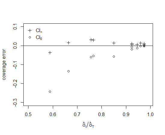
When is near , the behaviors (coverage and width) of and are similar and both have coverage close to the nominal level; this is illustrated in Figure 3. Recall that does not account for metamodel uncertainty, and that indicates that input uncertainty is large relative to metamodel uncertainty, which is when will do best. Figure 3 also illustrates the general robustness of .
6.3 Robustness to Unstable Moments
Recall the observation from Table 2 that when there is a small quantity of real-world data (), resulting in a large probability of unstable bootstrap moments, then both and had large mean and SD of their widths, yet provided reasonable coverage. Examining the results, we found that most of the intervals that fail to cover the mean do so because the lower confidence bound is above ; this is the case for both and . Using all 1000 macro-replications, the estimated probability that the lower confidence bound is above the mean (greater than , meaning too large) is 4.4% for and 3.8% for , while the estimated probability that the upper confidence bound is below the mean (less than , meaning too small) is only for and for ; for two-sided equal percentile intervals we would expect these to be around .
We conclude that even though the metamodel predicts a finite mean when it should be infinite, this will still tend to lead to overcoverage rather than undercoverage, and therefore is conservative.
7 Conclusions
In this paper, a metamodel-assisted bootstrapping approach is used for statistical uncertainty analysis. Input uncertainty is approximated by the bootstrap, an equation-based stochastic kriging metamodel is used to propagate the input uncertainty to the output mean, and the metamodel uncertainty is derived using properties of stochastic kriging. This approach delivers an interval estimator that accounts for all statistical uncertainty, both simulation and input. The asymptotic consistency of this interval is proved under the assumption that the true response surface is a realization of a Gaussian process and certain parameters are known.
An empirical study on a difficult problem demonstrates that our approach can have good finite-sample performance even when there are several input distributions (both discrete-valued and continuous-valued), a tight computational budget, and bootstrap moments corresponding to unstable systems. Thus, the new interval does not require a sequential experiment to make metamodel uncertainty negligible, as in Barton et al. (2014).
If is too wide, then it is important to know the relative contributions from input and metamodel uncertainty as a guide to either collecting more real-world data or doing more simulation or both. We give a measure of the relative contribution of input to overall statistical uncertainty by using a variance decomposition and analyze its asymptotic properties.
Acknowledgments
This paper is based upon work supported by the National Science Foundation under Grant Nos. CMMI-0900354 and CMMI-1068473. The authors thank Ohad Perry, the associate editor and two anonymous referees for their help in the presentation of results and certain technical issues.
References
- Adler ((2010)) Adler, R.J. (2010). The geometry of random fields. Philadelphia, PA: SIAM.
- Ankenman & Nelson ((2012)) Ankenman, B.E. & Nelson, B.L. (2012). A quick assessment of input uncertainty. In Proceedings of the 2012 winter simulation conference (p. 241-250). : Piscataway, New Jersey: Institute of Electrical and Electronics Engineers, Inc.
- Ankenman et al. ((2010)) Ankenman, B.E., Nelson, B.L. & Staum, J. (2010). Stochastic kriging for simulation metamodeling. Operations Research 58 371-382.
- Bangerth et al. ((2006)) Bangerth, W., Klie, H., Wheeler, M.F., Stoffa, P.L. & Sen, M.K. (2006). On optimization algorithms for the reservoir oil well placement problem. Computational Geosciences 10 303-319.
- Barton ((2007)) Barton, R.R. (2007). Presenting a more complete characterization of uncertainty: Can it be done? In Proceedings of the 2007 informs simulation society research workshop. Fontainebleau: .
- Barton et al. ((2014)) Barton, R.R., Nelson, B.L. & Xie, W. (2014). Quantifying input uncertainty via simulation confidence interval. Informs Journal on Computing 26 74-87.
- Barton & Schruben ((1993)) Barton, R.R. & Schruben, L.W. (1993). Uniform and bootstrap resampling of input distributions. In Proceedings of the 1993 winter simulation conference (p. 503-508). : Piscataway, New Jersey: Institute of Electrical and Electronics Engineers, Inc.
- Barton & Schruben ((2001)) Barton, R.R. & Schruben, L.W. (2001). Resampling methods for input modeling. In Proceedings of the 2001 winter simulation conference (p. 372-378). : Piscataway, New Jersey: Institute of Electrical and Electronics Engineers, Inc.
- Billingsley ((1995)) Billingsley, P. (1995). Probability and measure. New York: Wiley-Interscience.
- Chen et al. ((2012)) Chen, X., Ankenman, B.E. & Nelson, B.L. (2012). The effects of common random numbers on stochastic kriging metamodels. ACM Transactions on Modeling and Computer Simulation 22 7.
- Cheng & Holland ((1997)) Cheng, R.C.H. & Holland, W. (1997). Sensitivity of computer simulation experiments to errors in input data. Journal of Statistical Computation and Simulation 57 219-241.
- Cheng & Holland ((2004)) Cheng, R.C.H. & Holland, W. (2004). Calculation of confidence intervals for simulation output. ACM Transactions on Modeling and Computer Simulation 14 344-362.
- Chick ((2001)) Chick, S.E. (2001). Input distribution selection for simulation experiments: Accounting for input uncertainty. Operations Research 49 744-758.
- Chick & Ng ((2002)) Chick, S.E. & Ng, S.H. (2002). Joint criterion for factor identification and parameter estimation. In Proceedings of the 2002 winter simulation conference (p. 400-406). : Piscataway, New Jersey: Institute of Electrical and Electronics Engineers, Inc.
- Den Hertog et al. ((2006)) Den Hertog, D., Kleijnen, J.P.C. & Siem, A.Y.D. (2006). The correct Kriging variance estimated by bootstrapping. Journal of the Operational Research Society 57 400-409.
- Fowler & Rose ((2004)) Fowler, J.W. & Rose, O. (2004). Grand challenges in modeling and simulation of complex manufacturing systems. Simulation 80 469–476.
- Ghosh et al. ((2011)) Ghosh, S., Matsuoka, Y., Asai, Y., Hsin, K-Y. & Kitano, H. (2011). Software for systems biology: From tools to integrated platforms. Nature Reviews Genetics 12 821-832.
- Horowitz ((2001)) Horowitz, J.L. (2001). The bootstrap ( 5). Oxford, UK: North Holland.
- Jones et al. ((1998)) Jones, D., Schonlau, M. & Welch, W. (1998). Efficient global optimization of expensive black-box functions. Journal of Global Optimization 13 455-492.
- Kastner et al. ((2002)) Kastner, J., Solomon, J. & Fraser, S. (2002). Modeling a hox gene network in silico using a stochastic simulation algorithm. Developmental Biology 246 122-131.
- Kleijnen ((2008)) Kleijnen, J.P.C. (2008). Design and analysis of simulation experiements. New York: Springer.
- Lehmann & Casella ((1998)) Lehmann, E. & Casella, G. (1998). Theory of point estimation. New York: Springer-Verlag.
- Loeppky et al. ((2009)) Loeppky, J.L., Sachs, J. & Welch, W.J. (2009). Choosing the sample size of a computer experiment: A practical guide. Technometrics 51 366-376.
- Ng & Chick ((2006)) Ng, S.H. & Chick, S.E. (2006). Reducing parameter uncertainty for stochastic systems. ACM Transactions on Modeling and Computer Simulation 16 26-51.
- Picheny et al. ((2010)) Picheny, V., Ginsbourger, D., Roustant, O., Haftka, R.T. & Kim, N. (2010). Adaptive designs of experiments for accurate approximation of a target region. Journal of Mechanical Design 132 071008.
- Santner et al. ((2003)) Santner, T.J., Williams, B.J. & Notz, W.I. (2003). The design and analysis of computer experiments. New York: Springer.
- Serfling ((2002)) Serfling, R.J. (2002). Approximation theorems of mathematical statistics. New York: Wiley.
- Severini ((2005)) Severini, T. (2005). Elements of distribution theory. New York: Cambridge University Press.
- Shao & Tu ((1995)) Shao, J. & Tu, D. (1995). The jackknife and bootstrap. New York: Springer.
- Song & Nelson ((2013)) Song, E. & Nelson, B.L. (2013). A quicker assessment of input uncertainty. In Proceedings of the 2013 winter simulation conference (p. 474-485). : Piscataway, New Jersey: Institute of Electrical and Electronics Engineers, Inc.
- Sun & Farooq ((2002)) Sun, H. & Farooq, M. (2002). Note on the generation of random points uniformly distributed in hyper-ellipsoids. In Proceedings of the fifth international conference on information fusion (p. 489-496).
- Van Der Vaart ((1998)) Van Der Vaart, A.W. (1998). Asymptotic statistics. Cambridge, UK: Cambridge University Press.
- Wang et al. ((2012)) Wang, H., Ciaurri, D.E., Durlofsky, L.J. & Cominelli, A. (2012). Optimal well placement under uncertainty using a retrospective optimization framework. SPE Journal 17 112-121.
- Wieland et al. ((2003)) Wieland, J.R., Pasupathy, R. & Schmeiser, B.W. (2003). Queueing-network stability: Simulation-based checking. In Proceedings of the 2003 winter simulation conference (p. 520-527). : Piscataway, New Jersey: Institute of Electrical and Electronics Engineers, Inc.
- Xie et al. ((2010)) Xie, W., Nelson, B.L. & Staum, J. (2010). The influence of correlation functions on stochastic kriging metamodels. In Proceedings of the 2010 winter simulation conference (p. 1067-1078). : Piscataway, New Jersey: Institute of Electrical and Electronics Engineers, Inc.
- Zouaoui & Wilson ((2003)) Zouaoui, F. & Wilson, J.R. (2003). Accounting for parameter uncertainty in simulation input modeling. IIE Transactions 35 781-792.
- Zouaoui & Wilson ((2004)) Zouaoui, F. & Wilson, J.R. (2004). Accounting for input-model and input-parameter uncertainties in simulation. IIE Transactions 36 1135-1151.
8 Appendix (Intended for an Online Companion)
In this appendix we prove Theorems 1–3 and provide a brief description of the experiment design used to build stochastic kriging metamodels.
To be self-contained, we first state some definitions, lemmas and theorems that are used in the proofs. Let denote convergence in distribution.
- •
Borel-Cantelli Lemma (Billingsley (1995)): For events , if converges, then
where
is the set of outcomes that occur infinitely many times.
- •
Lemma 2.11 (Van Der Vaart (1998)): Suppose that for a random vector X with a continuous distribution function. Then the distribution function of converges uniformly to that of X: , where is the sup-norm of on , .
- •
Portmanteau Lemma (Van Der Vaart (1998)): For any random vectors and the following statements are equivalent.
- 1.
- 2.
for all bounded, continuous functions .
- 1.
- •
Theorem 2.3 (Van Der Vaart (1998)): Let be continuous at every point in a set such that . Then
- 1.
If then .
- 2.
If then .
- 3.
If then .
In the proofs when we refer to the “continuous mapping theorem” we will mean Theorem 2.3.
- 1.
- •
Glivenko-Cantelli Theorem (Van Der Vaart (1998)): If are i.i.d. random variables with distribution function and is the empirical cdf of , then as .
- •
Lemma 21.2 (Van Der Vaart (1998)): For cdf , define the inverse cdf to be
Then a sequence of cdfs for every where is continuous if and only if for every where is continuous.
- •
Theorem 13.1 (Severini (2005)): Let denote a sequence of -dimensional random vectors such that, for some vector ,
where is a positive definite matrix with . Let denote a continuously differentiable function and let denote the matrix of partial derivatives of with respect to . Then
- •
Theorem 3.8 (Shao & Tu (1995)): Let denote -dimensional i.i.d. random vectors and . Let where are randomly and independently drawn with replacement from . Let denote a continuously differentiable function and denote the matrix of partial derivatives of with respect to . Let and denote the bootstrap variance estimator for by .
Suppose that and where . Suppose further that
(17) where the maximum is taken over all integers satisfying , and is a sequence of positive numbers satisfying and with a Then is strongly consistent, i.e., , where and
- •
Theorem 1.1 (Lehmann & Casella (1998), Chapter 6): Let be i.i.d. with , , and finite fourth moment, and suppose is a function of a real variable whose first four derivatives and exist for all , where is an interval with . Furthermore, suppose that for all , for some . Then
If, in addition, the fourth derivative of is also bounded, then
In both cases the remainder is .
- •
Multivariate Taylor Formula (Serfling (2002), page 44): Let the function defined on posses continuous partial derivatives of order at each point of an open set . Let . For each point , , such that the line segment joining and lies in , there exists a point in the interior of such that
8.1 Asymptotic Consistency of
To prove Theorem 1, we first establish three supporting lemmas.
Lemma 8.1.
Suppose that Assumptions 1–2 hold. Then the bootstrap resampled moments converge almost surely to the true moments as .
Proof: Since all of the input processes are independent, we establish the result for one input distribution without loss of generality. We prove the result for being the generic th-order moment, , for .
The th-order bootstrap resampled moment is
| (18) |
where “” denotes the th independent sample with replacement from . We use the Chebychev Inequality and the Borel-Cantelli Lemma to prove the result.
By the Chebychev Inequality, for every , we have
| (19) |
Notice that
| (20) |
We will analyze each term in Equation (20). First, we show that any th bootstrap resampled moment, denoted as , is unbiased,
| (21) | |||||
Thus, . Notice that
where means terms at most order . Similar derivations show that
and
Thus,
| (22) | |||||
because all of the terms cancel. Therefore, combining Equations (19), (20) and (22), we have
where is some finite constant. Thus, if , then by the first Borel-Cantelli Lemma in Section 4 of Billingsley (1995).
Since Assumption 2 guarantees for each moment associated with the th input distribution, we can generalize the almost sure convergence to a vector of moments by applying the converging together lemma. Therefore, we have .
Remark: The independent variables in our stochastic kriging metamodel consist of central moments and standardized central moments. Since standardized moments are continuous functions of raw moments, we can use the continuous mapping theorem to obtain corresponding almost sure convergence of the standardized moments.
Given a fixed and finite number of design points , let . The simulation error at design point is , so let for denote the average. Therefore, the sample means of simulation outputs at all design points can be represented as , where . Finally, let be a GP having the conditional distribution of given .
Lemma 8.2.
Suppose Assumptions 3–4 hold. Then has continuous sample paths almost surely.
Proof: Let be the underlying probability space for the GP , and be the underlying probability space for . Notice that depends on the particular design points and corresponding numbers of replications which we consider fixed and given, while does not.
Let be an elementary outcome and the resulting random function. For notational convenience, let the random function evaluated at . Similarly, for elementary outcome . Notice that under Assumption 3, has a multivariate normal distribution.
Theorem 3.4.1 of Adler (2010) asserts that there is a -measurable set such that , and for every the function is continuous.
The random variable maps as for with probability measure since they are independent. Our goal is to prove that
| (23) |
almost surely.
Lemma 8.3.
Suppose that Assumptions 1–4 hold. Then as .
Proof: Under Assumption 3, the GP has continuous sample paths almost surely; applying Lemma 2, also has continuous sample paths almost surely. Under Assumptions 1–2, as by Lemma 1. And and are independent. The result follows by applying the continuous mapping theorem.
Theorem 8.1.
Suppose that Assumptions 1–4 hold. Then the interval is asymptotically consistent, meaning
| (24) |
Proof: Define Notice that the distribution depends on both the distributions of and . Specifically,
Thus, is a continuous distribution almost surely. Let be the empirical cdf of , which are i.i.d. from . Notice that for and .
By the Glivenko-Cantelli Theorem (Van Der Vaart (1998)), as . Therefore, by Lemma 21.2 of Van Der Vaart (1998),
as for . As a result,
Therefore, Equation (24) becomes
| (25) |
Since, conditional on , , the cdf is continuous. By Lemma 3 and Lemma 2.11 in Van Der Vaart (1998),
8.2 Asymptotic Analysis of Variance Component Estimators
Theorem 8.2.
Suppose that Assumptions 1–4 hold. Then the variance component estimators are consistent as .
Proof: When a GP has a continuous correlation function with all parameters finite, the SK predictor
| (27) |
and corresponding variance
where and , are continuous and bounded functions of .
By the Strong Law of Large Numbers, the raw moment estimator as under Assumptions 1–2. This almost sure convergence can be extended to central moments and standardized central moments by the continuous mapping theorem. By applying the Portmanteau Lemma in Van Der Vaart (1998), we have
and
where .
Recall that is a normal distribution . Let . Then
However,
Since and are continuous and bounded functions, so is . Therefore,
by applying the Portmanteau Lemma.
Next, we will show consistency of the variance estimators. By Lemma 1, For the metamodel uncertainty estimator, we have
The last step follows by applying the Portmanteau Lemma.
For the input uncertainty estimator, we have
The last step follows by applying Lemma 1 and the Portmanteau Lemma.
For the total variance estimator, we have
| (28) | |||||
By Lemma 3, . Then Step (28) follows by applying Portmanteau Lemma.
Theorem 8.3.
Suppose that Assumptions 1–4 and the following additional assumptions hold:
- 5.
The first three derivatives of the correlation function of the GP exist and the third derivative is bounded; and
- 6.
for .
Then almost surely, where is a positive constant.
Proof: Under Assumptions 1–2, and applying the multivariate central limit theorem, we have as ,
where denotes the positive definite asymptotic variance-covariance matrix of .
When a GP has a continuous correlation function with all parameters finite, the SK predictor
| (29) |
given the simulation sample mean , is continuous and bounded. Under Assumption 5, the gradient exists and is continuous. We will show that almost surely. By taking the derivative of in Equation (29), we have
| (30) |
Since and is positive definite, is a non-zero constant vector. Under Assumption 3, is a normal random variable that is equal to 0 with probability 0. Thus, almost surely. Applying Theorem 13.1 in Severini (2005), we have
where . This establishes the constant.
Since is continuous and bounded, there always exists a finite such that for all . Therefore, . Let . Since as , Condition (17) of Theorem 3.8 of Shao & Tu (1995) holds. Thus, the bootstrap variance estimator is strongly consistent: almost surely.
Next, we will show by proving a multi-variate version of Theorem 1.1 in Lehmann & Casella (1998), Chapter 6. Let denote the line segment joining and . By the Multivariate Taylor Formula (Serfling (2002)),
The remainder term
where denotes a value in the interior of , and and denote the th components of the vectors and . By taking the expectation over both sides, we have
| (31) |
where is the Hessian operator.
We will show that the second and third terms on the RHS of Equation (31) are and , respectively, under Assumption 5. Since all of the input processes are independent, we establish the result for one input distribution without loss of generality.
We prove the result for being the generic th-order moment, , and for .
Let . We first consider components of the second term on the RHS of Equation (31).
The last two steps follow because the are i.i.d. and Assumption 5 holds. Thus, the second term on the RHS of Equation (31) is
Similarly, for the components of the third term of the RHS of Equation (31), we have
where
Again, the last two steps follow because the are i.i.d. and Assumption 5 holds. Thus, the third term in Equation (31) is
Squaring both sides of Equation (31), we have
| (32) |
By repeating the same derivation that results in Equation (31) but using instead of , we obtain
| (33) | |||||
Then,
| (34) | |||||
Step (34) follows because is a scalar. Thus, we have .
Remark: The independent variables in our stochastic kriging metamodel consist of central moments and standardized central moments, rather than raw moments. However, Theorem 3 can easily be extended to central and standardized central moments as follows.
Since standardized moments are continuous functions of raw moments, denoted generically as , we can consider the composite function and follow steps analogous to those in the proof of Theorem 3. Up to the third derivatives we have
Let denote the mean, denote the th order raw moment and denote the th order central moment. Then the first three central moments can be expressed as functions of raw moments as follows:
The first three standardized central moments are and . For a non-degenerate distribution, the second central moment is positive and bounded away from . Thus, the first three derivatives exist and are finite.
8.3 Experiment Design
To fit SK metamodels we recommend the experiment design developed in Barton et al. (2014) which demonstrated robust performance over a number of test examples. In this section, we briefly review the basic methodology; for detailed information please refer to Barton et al. (2014).
The experiment design is not specified a priori; instead the design space, denoted by , depends on the real-world data that will eventually be resampled. In this way the design is adaptive.
At a high level, this is the approach: Generate a large number of bootstrap samples from the real-world data and compute the corresponding sample moments. Find a regular region that encompasses a large fraction of this sample; this will be the design space. Generate additional bootstrap samples to test that the regular region does indeed cover the desired fraction of the feasible space of sample moments, and refine if necessary. Once satisfied, embed a space-filling design in the regular region. These design points correspond to input distribution moments at which to run simulation experiments to fit the SK metamodel. We provide some more details below.
Suppose we are interested in a CI; we set in our empirical study. We want the experiment design to lead to a metamodel that is accurate for moments that are the most likely bootstrap moment vectors generated from ; by “likely” we mean, for instance, covering of the feasible bootstrap moments.
To this end we find an ellipsoid that will contain an independent bootstrap moment vector obtained by random sampling from with probability at least . We then generate a space-filling experiment design inside this ellipsoid. The procedure for constructing the design is as follows:
- 1.
Generate bootstrap resamples from and compute the corresponding sample moments to generate a set of sample moments .
- 2.
Find the smallest ellipsoid such that it contains the fraction of the data in when the ellipsoid’s center and shape are the sample mean and covariance matrix, respectively, of the elements of .
- 3.
Perform a hypothesis test where the null hypothesis is that a bootstrap moment will be contained in this ellipsoid with probability at least . This requires computing the number of bootstrap moment resamples, denoted by , and the constant that defines the rejection region to attain the desired Type I error and power for the test.
- 4.
Generate additional independent bootstrap resamples from and compute the moments . If more than of these resamples are contained in the ellipsoid, then accept the current as the design space. Otherwise, add these bootstrap resamples to , let and go to Step 2 to update the ellipsoid.
- 5.
Generate space-filling design points in the ellipsoid . To place design points into this space, we employ an algorithm due to Sun & Farooq (2002), §3.2.1, for generating points uniformly distributed in an ellipsoid. The algorithm first generates the polar coordinates of a point uniformly distributed in a hypersphere, then transforms it to Cartesian coordinates, and finally transforms it again to a point uniformly distributed in an ellipsoid. The advantage of this approach is that each element of the initial polar coordinates are independently distributed, allowing them to be generated coordinate by coordinate via their inverse cumulative distribution function. Rather than use randomly chosen points, however, we begin with a Latin hypercube sample on .
- 6.
Assign replications to each design point, where denotes total computational budget. Together the transformed Latin hypercube design points and the number of replications define the experiment design .
In our experiments we set Type I error of the hypothesis test to and its power to when the true probability is .
8.4 Sensitivity of Inference to SK Parameter Estimation Error
Since the parameters are unknown, we use estimators to form a SK metamodel. However, the properties of SK, and in particular Theorems 1–3, have only been established when at least are known. Nevertheless, kriging and SK have been observed to provide robust inference without accounting for parameter-estimation error provided we employ an adequate experiment design. Here we report a small-scale empirical study that examines parameter sensitivity for our particular problem: forming an ACI for and assessing the relative contribution of input uncertainty.
When we use the plug-in estimator , we get an unbiased SK predictor and small variance inflation, based on results in Ankenman et al. (2010). Therefore, we focus on sensitivity to the parameters . These parameters are estimated by maximum likelihood using the log-likelihood function
where is a function of and . The only random variable in the log-likelihood is , and the estimation uncertainty of the MLE is a complex function of the sampling distribution of (the contribution to uncertainty due to is tractable).
To study the sensitivity of our ACI to the estimation error of , we again use the queueing network example in Section 6. In each macro-replication, we generate real-world observations from each input model, find design points and run simulations to obtain and , now denoted by and . Then we compare the performance of our method under two settings:
- Case 1:
-
Use and to compute the MLEs for , use them to build the SK metamodel and construct CI+ as before (Section 5.1).
- Case 2:
-
Using the same experiment design, draw another independent sample of simulation outputs to obtain and , denoted by and , and obtain the corresponding MLEs . Use these estimates along with and to build the metamodel and again construct CI+.
Notice that in Case 2 we are obtaining GP parameter estimates from a sample of data that is independent of the data that forms the metamodel.
Table 4 shows the coverage and contribution results based on 1000 macro-replications. The nearly identical performance of Cases 1 and 2 demonstrates that our procedure is not sensitive to SK parameter estimation error if we employ the one-stage space-filling design used in the paper.
| , | Case 1 | Case 2 | ||||
| Coverage of | 95.6% | 97.9% | 96.4% | 95.5% | 98.1% | 95.5% |
| Width (mean) | 340 | 29.4 | 4.6 | 340 | 29.3 | 4.4 |
| Width (SD) | 171 | 18.8 | 0.93 | 170 | 18.8 | 0.91 |
| 0.972 | 0.960 | 0.925 | 0.971 | 0.963 | 0.922 | |