Minimal controllability problems on linear structural descriptor systems
Abstract
We consider minimal controllability problems (MCPs) on linear structural descriptor systems. We address two problems of determining the minimum number of input nodes such that a descriptor system is structurally controllable. We show that MCP0 for structural descriptor systems can be solved in polynomial time. This is the same as the existing results on a typical structural linear time invariant (LTI) systems. However, the derivation of the result is considerably different because the derivation technique of the existing result cannot be used for descriptor systems. Instead, we use the Dulmage–Mendelsohn decomposition. Moreover, we prove that the results for MCP1 are different from those for usual LTI systems. In fact, MCP1 for descriptor systems is an NP-hard problem, while MCP1 for LTI systems can be solved in polynomial time.
Index Terms:
structural controllability, large-scale system, descriptor system, DM decompositionI Introduction
Controllability, which was introduced by [kalman1960general], for network dynamical systems such as multi-agent systems[mesbahi2010graph], brain networks[gu2015controllability], and power networks[pagani2013power] has received considerable research attention. In the simplest case, systems can be modeled as linear time invariant (LTI) systems with state and input ,
| (1) |
where and are large constant matrices. In control theory literature, qualitative and quantitative controllability problems of designing under some constraints have been considered. The qualitative problem includes a problem that makes system (1) controllable with minimum input nodes [liu2011controllability, olshevsky2015minimal, pequito2015framework, olshevsky2015minimum] by employing a structural control theory developed in [lin1974structural, shields1976structural]. In contrast, the quantitative problem includes the problem of maximizing some metrics of the system; in particular, the controllability Gramian [summers2015submodularity, pasqualetti2014controllability, sato2020controllability, yan2015spectrum]. In a real-world system, each parameter in and is usually not precisely determined; further, the quantitative problem often becomes computationally difficult as the state dimension becomes larger. That is, we can only handle up to a few hundred state dimensions in practice. Thus, considering the qualitative problem is more suitable for large-scale networked systems.
To address the controllability problem of large-scale networked systems, we consider the qualitative problems called minimal controllability problems (MCPs)[olshevsky2015minimal]. The MCP0 is a problem that finds an matrix such that system (1) is structurally controllable and is minimum. Here, system (1) is called structurally controllable if system (1) becomes controllable by setting nonzero values in and [lin1974structural]. The MCP1 is a problem that finds an diagonal matrix such that system (1) is structurally controllable and the number of nonzero elements in is minimum. Although both MCP0 and MCP1 can be seen as a problem of minimizing the number of input nodes, each input in the MCP1 case is not allowed to connect to multiple nodes (the visual difference is shown in Fig. 1). Polynomial time algorithms for MCP0 and MCP1 associated with system (1) were proposed in [liu2011controllability, pequito2015framework, olshevsky2015minimum], respectively.
In this paper, we extend the results of [liu2011controllability, pequito2015framework, olshevsky2015minimum] on MCPs for a descriptor system
| (2) |
which is a generalized system of system (1), where can be a singular matrix. The descriptor formulation is well suited to model practical systems with algebraic constraints such as electric circuit systems [dai1989singular, murota00, duan2010analysis]. The structural controllability of descriptor system (2) is investigated by [yamada1985generic, yip1981solvability]; however, there is less discussion in terms of the input selection problem. In fact, to the best of our knowledge, the input selection problem based on structural controllability for descriptor system (2) is only found in [clark2017input]. However, [clark2017input] only deals with a special case in (2), as explained in Section II-C.
 (a) MCP0
 (b) MCP1
|
The contributions of this study can be summarized as follows.
- •
We provide the solution of MCP0 for structural descriptor system (2). The solution shows that the minimum number of input nodes is determined by maximum matching. This is the same as the result in [liu2011controllability]. However, the derivation is different from that in [liu2011controllability] based on graph concepts such as cacti. This is because a directed graph representation cannot be applied to descriptor system (2) unlike LTI system (1), as explained in Section II-B. Thus, instead of the graph concepts used in [liu2011controllability], we use a bipartite graph representation and the Dulmage–Mendelsohn (DM) decomposition [dulmage1963two][murota00] for descriptor system (2).
- •
We prove the computational hardness of MCP1 for structural descriptor system (2). That is, we show that the time complexity belongs to the NP-hard class by reducing the set cover problem, which is an NP-hard problem, to MCP1 for an instance of structural descriptor system (2). The result is completely different from that for system (1), which can be solved in polynomial time.
The remainder of this paper is organized as follows. Section II describes the results of previous studies on MCPs. The formulation of the novel MCPs for structural descriptor systems is described in Section III. In Section IV, we provide the analysis of the MCPs for system (2). The conclusions are presented in Section .
II Previous results of the MCPs
This section describes the existing MCPs results to highlight the difference with our study.
II-A Basic concepts of graph theory
We summarize the basic concepts of graph theory that are used in this study.
A strongly connected component (SCC) for a directed graph with nodes set is a maximal subset whose nodes can be connected by a directed path on the graph (Fig. 2). A directed matching of a directed graph with edges set is a subset that does not share common start or end nodes. Directed matching with the maximum size is called maximum directed matching.
For a bipartite graph , and with edge denote the nodes of and , respectively. Edges set is matching if it does not share the end of each edge. A matching is called maximum matching if contains the largest possible number of edges (Fig. 3). If all nodes are ends of some edges in a maximum matching , is called perfect. For a matching of , the elements of and are called right-unmatched nodes and left-unmatched nodes, respectively.


II-B Results of MCPs on system (1)
We first introduce the results of MCPs for structural system (1). MCP0 and MCP1 as mentioned in Section I can be formulated as
where denotes the number of nonzero elements of a matrix, and and denote the set of all generic matrices and generic vectors, respectively. A matrix is called generic if each nonzero element is an independent parameter. For a more precise definition of the generic matrix, see [murota00].
To provide the solution to MCPs, we define a directed graph representation of system (1), which is the fundamental tool for structural system analysis. The nodes set with
| (3) | ||||
| (4) |
corresponds to the state and input variables, and an edge set is defined as with and . Here, represents the connections between state nodes and represents connections between the state and input nodes. A digraph representation of the autonomous system (1) with is defined as .
The minimum number of input nodes , i.e., the optimal value of MCP0, is obtained by finding the maximum directed matching of [liu2011controllability]
where denotes the maximum directed matching of . The maximum directed matching of can be calculated as the maximum bipartite matching by translating to a corresponding bipartite graph . The node sets and are defined as and with and . The elements of and correspond to the column and row numbers of , respectively. In addition, the edge set is defined as , where and . Then, the maximum directed matching of can be regarded as the maximum matching of by identifying and of . Moreover, the minimum input nodes in MCP0 correspond to the left-unmatched nodes of a maximum matching of .
To describe the solution to MCP1, we note that the optimal value of MCP1 is given as , which was shown in [pequito2015framework], where denotes the number of left-unmatched nodes in any maximum matching of the bipartite graph , and denotes the number of root SCCs, that have no incoming links from other SCCs. A top assignable SCC is a root SCC that contains at least one left-unmatched node associated with a maximum matching , and is the maximum number of top assignable SCCs. This maximum top assignability index can be calculated using the minimum weight maximum matching whose time complexity is . For more details, see [korte2012combinatorial]. A faster method for solving MCP1 using the minimum cost allowed matching is proposed by [olshevsky2015minimum]; its time complexity is .
II-C Results of MCPs on system (2)
The input selection problems that make descriptor system (2) structurally controllable are proposed in [clark2017input]. In [clark2017input], the authors studied the following special case of system (2) and the problem of minimizing the size of .
| (5) |
Moreover, they showed that this problem can be solved in polynomial time by formulating it as a matroid intersection problem
where and denote the duals of the matroid determined by the matrices of descriptor system (5). This is a special case of MCP1, as formulated in Section III because the inputs must be connected to state nodes directly. To the best of our knowledge, this is the only work on the minimum input selection for “structural” descriptor system (2), although the structural controllability analysis without considering input selections can be found in [murota00, yamada1985generic]. We address a more general MCP1 in this paper.
Unlike the problems in [clark2017input] and this study, [zhang2020sparsest] considered the input selection problems for non-structural descriptor system (2) formulated as
| (6) | ||||
| (7) |
where denotes an integer . That is, in contrast to the “structural” controllability problem in [clark2017input] and this paper, [zhang2020sparsest] addressed usual controllability problems. Moreover, the column size of in Problem (7) is given in advance, whereas MCP0 is the problem of minimizing the column size of . In [zhang2020sparsest], the authors showed that Problems (6) and (7) are NP-hard. These results are analogous to the NP hardness of MCPs for non-structural LTI systems [olshevsky2015minimal].
III Problem Settings
In this section, we formulate novel MCPs for descriptor system (2).
Because the controllability of system (2) is different from that for system (1), we first define the controllability for descriptor system (2) and describe the equivalent conditions.
We assume that system (2) is solvable, i.e., for any initial state with an admissible input , there exists a unique solution to Eq. (2). This condition is equivalent to
| (8) |
where is an indeterminant [murota00] [yip1981solvability].
Some definitions of the controllability[yip1981solvability] are provided in the descriptor system theory, as explained in Remark 1. In this paper, we call system (2) controllable if for any admissible initial state satisfing equation (2), there exists an input and a final time such that .
An algebraic characterization of the controllability is provided below [yip1981solvability, berger2013controllability]:
Proposition 1
Descriptor system (2) is controllable if and only if
| (9) |
In Proposition 1, the matrix is called the modal controllability matrix.
System (2) is called structurally controllable if condition (9) in Proposition 1 holds for (2) with generic matrices , , and . The generic matrices mean that all non-zero entries represent free parameters, which are algebraically independent [murota00].
We now formulate novel MCPs for descriptor system (2). MCP0 and MCP1 for descriptor system (2) can be formalized as
Although the -th row differential equation corresponds to for LTI system (1), there is no such correspondence because of the presence of for descriptor system (2). Therefore, the directed graph representation of the system in [liu2011controllability] cannot be applied. Thus, we cannot use the proofs of the theorems on MCP0 [liu2011controllability] and MCP1[pequito2015framework] for descriptor system (2) with generic matrices.
Remark 1
Controllability for descriptor systems has some variants, such as complete controllability, R-controllability, impulse controllability, and strong controllability[berger2013controllability]. Our controllability in this paper corresponds to R-controllability. For more detail, see [dai1989singular, berger2013controllability] and references therein.
IV Analysis of the MCPs
We analyze the MCPs for descriptor system (2) with generic matrices using a graph theoretic approach.
To this end, we first describe the graphical representation of descriptor system (2) with generic matrices and graph theoretical controllability.
Although there are several graph representations of descriptor system (2) [reinschke1997digraph, yamada1985generic, murota00], we use a bipartite graph representation and its DM decomposition proposed in [murota00]. The DM decomposition is explained in Appendix . This bipartite representation is considerably different from the bipartite graph for LTI system (1) described in Section II-B.
The bipartite graph associated with descriptor system (2) is defined as follows: the node sets and the edge set are defined as
| (10) |
with , and , where and are defined as (3) and (4), respectively, and corresponds to an -th row of system (2). An edge belonging to is called an s-arc. Further, we call a DM s-component for a DM component that has s-arcs. The symbol denotes the size of a maximum matching of . Let be DM components, and are called consistent DM conponents; and are called inconsistent DM components.
In [murota00], we find the following graph theoretic characterization of structural controllability for descriptor system (2).
Proposition 2
Descriptor system (2) is structurally controllable if and only if
- 1.
- 2.
- 3.
No consistent DM components contain s-arcs
where and .
Condition 1) represents the solvability of the system described in Eq. (8) in Section III, and the latter two conditions correspond to (9) in Proposition 1. From assumption (8), condition 1) in Proposition 2 is always satisfied. This means that there are no inconsistent components and of .
To illustrate 1), 2), and 3) in Proposition 2, consider an example of descriptor system (2) with
| (11) |
Then, the corresponding bipartite representation is shown in Fig. 4 (a). The maximum matching sizes for and are both 3, which means that conditions 1) and 2) in Proposition 2 hold. The graph is an inconsistent DM component and are consistent DM components; further, the partial order is introduced by and . In this case, does not exist because we can identify a maximum matching of as a perfect matching , that is, , where is defined in Appendix . This holds under the solvability (8) of descriptor system (2). This decomposition corresponds to the block diagonalization of the modal controllability matrix
That is, we can choose permutation matrices and make block the upper triangular matrix as
| (12) |
The diagonal block matrices are given as
Block matrices correspond to DM components . As can be seen from Fig. 4 (b) and Eq. (12), a consistent component has an s-arc. Thus, this system is not structurally controllable by condition 3) in Proposition 2 because is not driven by an input in the 1st equation of the system .
 (a)
(a)
 (b)
(b)
|
IV-A Analysis of the MCP0
In this subsection, we prove that in the MCP0 case, the minimum number of input nodes for descriptor system (2) coincides with that for LTI system (1).
Theorem 1 (minimum input theorem)
Proof
If has a perfect matching, that is , then condition 2) in Proposition 2 is automatically satisfied by using edges of in finding the maximum matching of for any . Moreover, adding a single input node and adding edges from to each s-consistent component, condition 3) in Proposition 2 is satisfied. Thus, the minimum number of input nodes is .
We assume that does not have perfect matching, that is . Let be the number of input nodes that the associated system (2) is structurally controllable and
| (14) |
From condition 2) in Proposition 2, holds. Let be a maximum matching of , and then, let be a matching of , and
| (15) |
From (14) and (15), . This contradicts the maximality of . Thus, . Let be the maximum matching of and a number of input nodes be . Connecting each input node to a node of , is satisfied, i.e., condition 2) in Proposition 2 holds. In addition, by connecting input nodes to s-consistent DM components of , 3) in Proposition 2 is satisfied without increasing the number of input nodes. The reason is as follows. From assumption (8) and the structure of , we can use the perfect matching of as the maximum matching of in the DM decomposition of . Hence, it follows from (10) that in the construction of the DM decomposition is just . Thus, all s-consistent DM components of become inconsistent DM components, and 3) in Proposition 2 is satisfied.
Therefore, system (2) constructed in the above manner is structurally controllable.
The statement of Theorem 1 for descriptor system (2) with generic matrices coincides with that of the minimum input theorem in Section II in [liu2011controllability] for LTI system (1) with generic matrices. In [liu2011controllability], the corresponding proposition was proved using graphical concepts such as cacti. However, we cannot use the concepts for descriptor system (2), because (2) cannot be represented by the directed graph as mensioned in Section III. Instead, we use condition 2) in Proposition 2, which denotes the controllability condition using the maximum bipartite matching. Moreover, the DM decomposition can be constructed in time [murota00]. Thus, we can construct as the solution to MCP0 for descriptor system (2) with generic matrices in polynomial time.
To demonstrate how to use this result, we consider autonomous descriptor system (2) with and defined in (11). Recall that . That is, condition 1) in Proposition 2 holds. Then, the maximum matching of is given as . Thus, and it follows from (13) that the minimum node size is . From the proof of Theorem 1, we must connect an input node to the left unmatched node . Then, condition 2) in Proposition 2 holds. Moreover, to satisfy condition 3) in Proposition 2, we must add an edge between and because the DM component of that contains has s-arcs (Fig. 5 (a)). Thus, we have a solution to MCP0 as
Then, the DM decomposition of the modal controllability matrix
is given as
where and are permutation matrices. The corresponding DM decomposition of the bipartite graph is shown in Fig. 5 (b). This shows that the DM components are , and the only consistent DM component has no s-arcs, whereas in Fig. 4 has an s-arc. Thus, from Proposition 2, system (2) is structurally controllable.
 (a)
(a)
 (b)
(b)
|
IV-B Intractability of MCP1 for descriptor systems
We prove that the set cover problem, which is an NP-hard problem, can be reduced to MCP1 for an instance of descriptor system (2) with generic matrices. This means that MCP1 for descriptor system (2) with generic matrices is NP-hard.
To this end, we first define additional terms of the DM components of descriptor system (2) and discuss permissible inputs under the assumption of MCP1 that only one state node can be connected to an edge from each input, as illustrated in the right of Fig. 1.
The maximal consistent DM s-component is a consistent DM s-component of such that no other DM s-components are greater than related to the partial order . For example, in Fig. 4 (b) is a maximal consistent DM s-component.
A subset is called an input configuration if system (2) becomes structurally controllable by connecting the inputs to the nodes specified by . An input configuration is a feasible solution to MCP1 for descriptor system (2). A similar yet slightly different concept of the input configuration can be found in [pequito2015framework] for LTI system (1) with generic matrices.
From the graphical condition of structural controllability in Proposition 2, we obtain the following theorem on the input configuration. This theorem clarifies the structure of the input configuration in MCP1 and reduces the set cover problem to MCP1 for an instance of system (2).
Theorem 2
A subset is an input configuration if and only if
where is the set of left unmatched nodes of a maximum matching of , i.e., . The symbol is a set whose nodes can reach all maximal s-consistent components. That is, for any maximal s-consistent component , there exists a node such that . Here, denotes the DM component of to which belongs.
Proof
Let be a generic diagonal matrix corresponding to the set .
() From the definition of , the system (2) with is structurally controllable. Then, holds from condition 2) in Proposition 2. If , there exists a maximum matching of and is unmatched nodes. This implies that must contain , and thus .
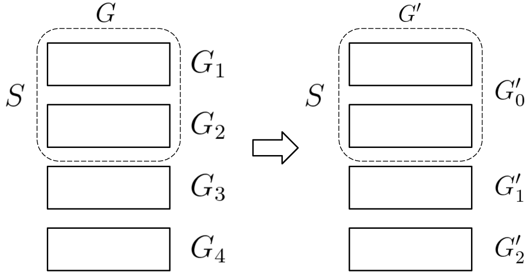
To show that must contain , we provide the relationship between the DM components of and , where and are defined in the beginning of Section IV. Let be the DM components of . From assumption (8), condition 1) in Proposition 2 holds. Thus, there are no inconsistent components . Then, the nodes sets of the DM components of are
That is, the DM component that contains the nodes of will be merged with the inconsistent DM component , and the other components remain consistent (Fig. 6). For to be merged to an inconsistent component in , an input node must exist and be connected to that is either or a larger (in the sense of the partial order of DM decomposition) consistent component. Combining this with condition 3) in Proposition 2, we have .
() Let contain , and let be a maximum matching of . Each input node specified by connects to the left-unmatched nodes of in the maximum matching . If we choose edges from and in finding a maximum matching of , holds. That is, condition 2) in Proposition 2 is satisfied. Moreover, from the definition of , all consistent s-components of become inconsistent components in the DM decomposition of . This means that no consistent components contain s-arcs; thus, descriptor system (2) with is structurally controllable. That is, is an input configuration.
We briefly discuss the set cover problem to prove the intractability of MCP1 for descriptor system (2) with generic matrices. Consider , and with . The set cover problem is a problem that finds the minimum size index such that covers .
| (16) |
The set cover problem is NP-hard as shown in Theorem 15.24 in [korte2012combinatorial].
The computational difficulty of MCP1 for descriptor system (2) with generic matrices can be proven using Theorem 2.
Theorem 3 (Intractability of MCP1 for descriptor system)
MCP1 for descriptor system (2) with generic matrices includes the set cover problem. That is, its computational complexity is NP-hard.
Proof
We show that given , , we can define a specific autonomous descriptor system (2) with corresponding to the set cover problem.
To this end, we first define a bipartite representation of the system. Its DM components correspond to the elements of and . Moreover, the order between a DM component associated with an element of and a subset can be regarded as the inclusion between and . The nodes sets and are defined as . Further, we define and . Then, the DM components of this bipartite representation are the subgraph induced by or . The DM components induced by and correspond to the element of and the subset , respectively. Moreover, if , the DM component induced by is less than the DM component induced by in the sense of the order of DM decomposition. It follows from (10) that the bipartite graph defines an instance of descriptor system (2) with .
Theorem 2 implies that the number of input configuration is
| (17) |
In this case, because we can take only a perfect matching from as a maximum matching , is fixed to . Combining this with (17), we have . Moreover, in the MCP1 case, we select as because we must select the minimum size of , which corresponds to a feasible solution to MCP1. Accordingly, MCP1 is equivalent to the following problem:
| (18) |
From the construction of , the s-consistent component corresponds exactly to the element of , and is chosen from any consistent components containing (Fig. ). Thus, problem (18) is equivalent to problem (16).
We explain Theorem 3 using Fig. . In MCP1 for LTI system (1), inputs must be connected to root SCCs. If a graph representation of system (1) is illustrated in the left of Fig. , then we must add two inputs. However, in MCP1 for descriptor system (2), if the maximal DM component contains no s-arc, and therefore, it must not be connected from inputs. Thus, we have to choose minimum inputs that cover all DM components that include s-arcs. Thus, the problem is more complicated. In [clark2017input], system (2) was restricted to the form given in Eq. (5) and a polynomial-time solution with a matroid intersection was proposed; however, our result shows that it is difficult to solve in polynomial time for a more general case.