Lipkin model on a quantum computer
Abstract
Atomic nuclei are important laboratories for exploring and testing new insights into the universe, such as experiments to directly detect dark matter or explore properties of neutrinos. The targets of interest are often heavy, complex nuclei that challenge our ability to reliably model them (as well as quantify the uncertainty of those models) with classical computers. Hence there is great interest in applying quantum computation to nuclear structure for these applications. As an early step in this direction, especially with regards to the uncertainties in the relevant quantum calculations, we develop circuits to implement variational quantum eigensolver (VQE) algorithms for the Lipkin-Meshkov-Glick model, which is often used in the nuclear physics community as a testbed for many-body methods. We present quantum circuits for VQE for two and three particles and discuss the construction of circuits for more particles. Implementing the VQE for a two-particle system on the IBM Quantum Experience, we identify initialization and two-qubit gates as the largest sources of error. We find that error mitigation procedures reduce the errors in the results significantly, but additional quantum hardware improvements are needed for quantum calculations to be sufficiently accurate to be competitive with the best current classical methods.
PhySH: Effective field theory, Particle dark matter, Quantum algorithms, Quantum information with solid state qubits, Many-body techniques, Nuclear many-body theory
I Introduction
Physics today finds itself in a conundrum. On one hand, the standard model of particle physics has been very successful. Yet from cosmological observations we are aware of how little we know. The makeup of the universe appears to be dominated by nonbaryonic dark matter Blumenthal et al. 1984; Primack et al. 1988; Feng 2010; Bertone and Hooper 2018 and so-called dark energy Frieman et al. 2008, and even the origin of the matter-antimatter imbalance in the Universe is not fully understood Dine and Kusenko 2003. While we understand the basic mechanisms of nucleosynthesis, the astrophysical site of a large fraction of heavy elements is still under debate Kajino et al. 2019.
Many of the experiments investigating these ongoing mysteries rely upon understanding detailed properties of atomic nuclei, from neutrinoless double -decay experiments searching for lepton number violation Dolinski et al. 2019, to detection of supernova neutrinos Mirizzi et al. 2016, to the direct detection of dark matter Schumann 2019. Because many of these experiments place upper limits, it is equally important to quantify the uncertainty in our models of those nuclei Cannoni 2013; Cerdeño et al. 2013; Furnstahl et al. 2015; Carlsson et al. 2016; Pérez et al. 2016; Yoshida et al. 2018.
With the advent of powerful computers and more rigorous techniques, as well as enhanced efforts in uncertainty quantification (UQ), our models of atomic nuclei have improved dramatically in the past two decades. Yet, like physics itself, we paradoxically see all too well the limits of our current computing platforms. Most of the targets for probing new physics are heavy, complex nuclei such as argon, germanium, or xenon; and uncertainty quantification can require many runs with small variations of parameters Furnstahl et al. 2015; Carlsson et al. 2016; Pérez et al. 2016; Yoshida et al. 2018; Fox et al. 2020. For these heavy nuclei, the exponential growth of the Hilbert space dimension makes calculations, especially multiple runs, challenging. In this context, the potential of quantum computers is appealing. Significant effort is already underway in applying quantum computers to problems with similar features such as quantum chemistry Hempel et al. 2018; Cao et al. 2019; Arute et al. 2020, the structure of atomic nuclei Dumitrescu et al. 2018; Roggero et al. 2020, and the structure of hadrons Kreshchuk et al. 2021; Mueller et al. 2020.
Useful progress towards implementing on quantum computers standard approximations such as configuration-interaction (CI) Babbush et al. 2017; Dumitrescu et al. 2018 and coupled clusters Ryabinkin et al. 2018; Romero et al. 2018 has been made. However, current quantum computers have much larger errors than classical computers, which must be taken into account when comparing the accuracy of predictions from approximate classical theories and the results of quantum calculations. Thus, our work here is a necessary first step in understanding the potential applications of quantum computing to nuclear structure needed to interpret experiments.
To start addressing quantum computation of models relevant to nuclear targets, we look at a simplified model of the many-body targets, the Lipkin-Meshkov-Glick (LMG or, colloquially, Lipkin) model Lipkin et al. 1965 where, because of symmetries, exact solutions are known and can be compared to quantum results. We present quantum circuits that can be used to implement variational quantum eigensolver (VQE) Peruzzo et al. 2014 algorithms for LMG models with different numbers of particles. We implement a VQE algorithm for a two-particle LMG model on the International Business Machines Corporation (IBM) Quantum Experience, a publicly available quantum computer, and identify the main sources of computational errors. We find that errors in measurement and in two-qubit gate operations are critical limitations. Implementation of error mitigation techniques Temme et al. 2017; Dumitrescu et al. 2018; He et al. 2020 provide significant improvement, though the remaining errors are not negligible. The analysis that we perform on the LMG model illustrates the current limitations of quantum computers and also identifies the improvements needed so that they can be able to provide results superior to those from classical machines.
The paper is organized as follows. In Sec. II we use the direct detection of dark matter as a case study, and discuss why quantum computers are potentially extremely useful. We then discuss how UQ is central to the comparison between quantum and classical computational approaches in a way relevant to experimental progress. In Sec. III we define the LMG model and show how its symmetry properties can be exploited to obtain analytic solutions for the ground state that can provide a benchmark for the results of quantum algorithms. In Sec. IV we present quantum circuits for determining the ground state of the LMG model using a VQE approach. In Sec. V we implement the algorithm for the smallest nontrivial case on the IBM Quantum Experience. We discuss the effects of different sources of infidelity in the calculation and their relative contributions to error in these VQE algorithms. We also explore the effectiveness of error mitigation techniques proposed in Refs. Temme et al. 2017; Dumitrescu et al. 2018; He et al. 2020 and show that the improvement in the accuracy of the calculations is substantial. In Sec. VI we give an example calculation of an observable as a forerunner of the kind of calculation one would need for actual applications. In Sec. VII we summarize our results and sketch further avenues for exploration.
II Dark Matter, Nuclear Structure, and Quantum Computing
Although there are many important applications of nuclear structure physics, here we use the direct experimental detection of dark matter as a case study. Recent observations in astrophysics and cosmology provide strong evidence that a large fraction of our Universe’s mass is composed of nonbaryonic dark matter Blumenthal et al. 1984; Primack et al. 1988; Feng 2010; Bertone and Hooper 2018. The direct detection of particle dark matter by measuring the recoil of nuclei that collide with dark matter particles would not only confirm this picture, it would demonstrate physics beyond the Standard Model Bertone et al. 2005; Jungman et al. 1996.
For many years dark matter interactions with baryonic matter were simply divided into coupling to the bulk (spin-independent) and coupling to the spin of quarks Sadoulet 1999; Goodman and Witten 1985, but recent theoretical developments Fitzpatrick et al. 2013; Anand et al. 2014; Vietze et al. 2015; Fieguth et al. 2018; Hoferichter et al. 2020 using effective field theory (EFT) techniques, have shown that the interpretation of direct detection experiments should be expanded to six (or more if one allows symmetry violation) nucleon-dark matter couplings.
These theoretical developments have important consequences for experimental design Alsum 2020. The target response to scattering of dark matter is computed by folding the single-nucleon reduced density matrix with the one-body matrix elements of operators derived in EFT. The relative sensitivity of experiments using different nuclear targets can vary by several orders of magnitude under changes in the underlying dark matter-nucleon coupling.
In addition, UQ has begun to be implemented into the theory of atomic nuclei Furnstahl et al. 2015; Carlsson et al. 2016; Pérez et al. 2016; Yoshida et al. 2018, based in part upon the realization that correct assessment of any experiment that rests upon models needs UQ Cannoni 2013; Cerdeño et al. 2013; Fox et al. 2020.
We have very good and predictive theories of nuclear structure, such as but not limited to the no-core shell model (NCSM), which is an ab initio CI method for the wavefunctions of atomic nuclei. The NCSM and other ab initio theories start from nucleon-nucleon scattering data and then, without further adjustment of parameters, calculate the structure and spectra of light nuclei Navrátil et al. 2000; Barrett et al. 2013. While in many aspects such calculations are very successful, the application of the NCSM has been limited largely to light nuclides, with mass number . Other ab initio methods such as coupled clusters can tackle heavier nuclei Hagen et al. 2010, but are mostly limited to near closed shells.
Alternatively, one can turn to phenomenological or empirical CI calculations Brussard and Glaudemans 1977; Brown and Wildenthal 1988; Caurier et al. 2005. Here one works in a restricted valence space. The interaction matrix elements, while starting from ‘realistic’ forces similar to those used in the NCSM, are adjusted to fit many-body spectra. Thus, phenomenological CI calculations have less rigorous foundations, when compared to the NCSM, and yet a greater range of applicability. (There are efforts to connect ab initio methods to phenomenological-like spaces with greater rigor and predictive power Stroberg et al. 2019, but those are still in development.) This comparison is particularly true with regard to medium- and heavy-mass nuclides of interest to the current generation of dark matter detectors.
Our challenge is that CI calculations Caurier et al. 2005 needed for dark matter calculations Pacheco and Strottman 1989; Ressell et al. 1993; Pirinen et al. 2016; Cannoni 2013; Cerdeño et al. 2013; Menéndez et al. 2012; Klos et al. 2013; Vietze et al. 2015; Baudis et al. 2013; Gazda et al. 2017 suffer from the exponential growth in the cost of storing the wavefunction classically. The largest CI calculations to date work in a basis space of dimension of the order . However, 40Ar, a key target in many experiments, if one works in a nuclear valence space of --- orbits, has a -scheme (fixed-) basis dimension of nearly 1015. Typically, one restricts excitations from the - orbits into the - orbits Hoferichter et al. 2019, but the results depend upon the specific truncation. For Xe isotopes, phenomenological calculations are generally in the restricted --- space. The most common isotope, 132Xe (with a natural abundance of ), requires a -scheme dimension of only , which can be calculated on a powerful laptop. The next most common isotope, 129Xe, has a basis dimension of , which can only be calculated on a supercomputer. 128Xe () has a basis dimension of , and 124Xe, rare yet also of interest to neutrinoless double-electron capture decay, has a -scheme basis dimension of , beyond the reach of current supercomputers.
For phenomenological calculations, UQ is both empirical and time-consuming. One varies the interaction parameters, of which there can be dozens or even hundreds, and recomputes the energies and other observables, in order to build up a model of the multi-dimensional error surface Yoshida et al. 2018; Fox et al. 2020. While this can be done in small model spaces where one can compute hundreds of observables in a few minutes, in larger spaces, where calculations of a single nuclide can take hundreds of CPU hours, such UQ analyses are daunting. Here is one example where even near-term quantum computers could be helpful in dramatically speeding up the many large calculations needed for UQ.
Quantum simulators have the potential to transform our ability to understand the performance of experiments, based on the ability of quantum simulators to calculate the properties of ground states of fermionic Hamiltonians much more efficiently than currently known classical algorithms. Performing these calculations using quantum computers is potentially advantageous because simulation of fermions is efficient Lloyd 1996 and does not suffer Clemente et al. 2020 from the “sign problem” that places severe limits on system sizes and/or temperatures achievable in fermionic calculations done using classical computers Loh et al. 1990.
A key question is how much reliable information can be obtained from current noisy quantum computers. To address this question, here we investigate a simplified model of targets that has symmetry properties enabling classical computers to determine the ground states of large systems; indeed, substantial analytic results are also available.
III Lipkin-Meshkov-Glick Model
To assess the validity of various quantum computational techniques, we calculate the ground state wave function of the LMG model Lipkin et al. 1965. The LMG model is widely used as a testbed for approximations in many-body physics, for example, time-dependent Hartree-Fock Krieger 1977, time-dependent coupled-clusters Hoodbhoy and Negele 1978; Wahlen-Strothman et al. 2017, the random phase approximation Stoica et al. 2001, generator coordinate methods Severyukhin et al. 2006, and density functional theory Lacroix 2009; Bertolli and Papenbrock 2008, a list which barely scratches the surface. It therefore strikes us as sensible to also use the LMG model as an early implementation of quantum computation.
In the LMG model Lipkin et al. 1965, fermions are distributed among two levels with -fold degeneracy and an energy separation of . Defining and as the creation and annihilation operators of the fermion in the state of level , we write the Hamiltonian of the system as
| (1) |
A term that scatters one fermion to the upper level and a second fermion to the lower level can also be added to this Hamiltonian, but such a term yields a constant in the SU(2) subspaces described below. Introducing the quasi-spin operators
| (2) | ||||
| (3) |
which span a SU(2) algebra, the LMG Hamiltonian can be rewritten as
| (4) |
One can calculate the expectation value of the Hamiltonian in Eq. (4) in the total quasispin basis. For a given , a matrix representing this operator has dimension , but it consists of blocks of matrices with SU(2) labels corresponding to different values obtained by adding SU(2) doublets. In the rest of this paper, we work with the dimensionless Hamiltonian with . Also we will only consider the multiplet with containing the unperturbed ground state.
It is especially convenient to write the Hamiltonian in the qubit basis. For particles, the total quasispin is given by
| (5) |
where each is in the representation. Hence, the Hamiltonian of Eq. (4) becomes
| (6) |
That is, the Hamiltonian matrix elements are: the sum of the values of the qubits () along the diagonal entries, the quantity when two qubits can be flipped, or zero otherwise.
IV Variational Quantum Eigensolver
In this section, we outline specific VQE algorithms for computation of the ground state of LMG models for generic values of and with fixed values of . We introduce the algorithm with the example of , for which we carry out calculations on quantum hardware and in noise simulations in later sections, and then present two directions for generalization of this method.
IV.1
We set up our algorithm by defining a dictionary basis to correspond to the quasi-spin basis; for example with : . In this basis the Hamiltonian is represented by
| (7) |
Here, , , and are the Pauli matrices. It is then straightforward to diagonalize this Hamiltonian to obtain the eigenvalues (with multiplicity 2) and . The normalized ground state with energy is given by
| (8) |
Here we consider a trial state that is a real superposition of the two states with total quasi-spin and :
| (9) |
defining a single variational parameter that can be optimized to minimize the value of . The state at which is the exact ground state, and so we restrict consideration of to the domain . In our VQE we optimize the value of by minimizing the expectation value of the energy evaluated on a quantum computer.
The state given by Eq. (9) can be prepared from an initial state by applying a one-qubit rotation about the axis of the Bloch sphere of a first qubit, written as
| (10) |
with , followed by a CNOT gate using the first qubit as the control and a second qubit as the target:
| (11) |
Here, , , and are the Pauli gates, , , . The quantum circuit for state preparation is summarized in Fig. 1.
The measurements on this quantum circuit needed to compute are simultaneous measurements in the basis for both qubits and in the basis for both qubits as well as measurements of each qubit in the basis. These measurements yield estimates of the expectation values , , , and , and thus determine from Eq. (6).
This procedure of writing the ground state wave function for particles as a real superposition controlled by a single trial parameter on a -qubit device may be generalized for higher values of , as we demonstrate in Sec. IV.2. However, first, let us briefly comment on the dimensionality of the ground-state Hilbert space within the LMG model. In general, the ground state will be a superposition of the state with all quasispins down and all states with any number pairs of quasi-spins flipped up. This parity is a symmetry that we can to exploit to reduce the cost of preparing a variational state and requiring only a single variational parameter. For this reason, we excluded both of the states with above, and so this dimension was simply 2 for the case . For general , this dimension will then be .
IV.2 Variational states for
In Sec. IV.1, we presented a quantum circuit to obtain a trial state with a single parameter to estimate the ground state of a LMG model for . Here, we generalize this approach to obtain variational wave functions for and .
IV.2.1 Trial state for
For , using the usual basis
the Hamiltonian is represented by
| (12) | |||||
Similar to Eq. (9) for , an appropriate variational ansatz for the ground state of is
| (13) |
where is the variational parameter. This wave function is the ground state when with energy , and so we restrict consideration of to the domain .
The three-qubit preparation circuit is shown in Fig. 2, written with two auxiliary angles and defined by
| (14) | ||||
| (15) |
IV.2.2 Trial state for
We can prescribe similarly a four-qubit trial state for the LMG model with . Here, the ground state belongs to the representation and has the energy . The unnormalized ground state wave function with this energy is
| (16) |
where
| (17) | ||||
| (18) |
After normalization one finds that the coefficients of and in Eq. (16) sum to 1. Therefore, we propose for a normalized trial state
| (19) |
with one variational parameter . The true ground state of the system is of this form with satisfying , and so we restrict consideration of to the domain .
We can continue this process for , establishing a trial wave function depending on one variational parameter for each . A common feature of these wave functions is that they all have definite parity. While a -qubit state of definite parity can be constructed from an associated -qubit state using an additional CNOT gates, the associated -qubit state will not in general have symmetries to exploit, and so a generic quantum state preparation routine is necessary to produce it. Using the quantum state preparation method of Ref. Plesch and Brukner 2011 to prepare the associated -qubit state, the CNOT cost of preparing an arbitrary -qubit state of definite parity is for even and for odd .
The next subsection presents a method for constructing quantum circuits that generate a particle variational state in a bosonic representation. Moreover, the method can be used to construct quantum circuits for generating the appropriate variational state for any .
IV.3 VQE circuits for
The LMG Hamiltonian can be rewritten in terms of bosonic operators acting on two bosonic modes Ortiz et al. 2005:
| (20) |
where and ( and ) are the creation and annihilation operators for a boson in the mode (), and are their number operators. For the bosonic representation, the number of particles is equal to the particle number of the fermionic representation Lerma H. and Dukelsky 2013.
Since the LMG model is exactly solvable any eigenstate of the LMG Hamiltonian can be written as the operator Ortiz et al. 2005
| (21) |
acting on bosonic fiducial state . The integer is related to and by , where are initially restricted to be or . For nonzero the spectral parameters are real numbers obtained by solving the Bethe ansatz equations Ortiz et al. 2005; Lerma H. and Dukelsky 2013
| (22) |
The two bosonic modes can be encoded in qubits up to a cutoff in occupation number by standard techniques Somma 2005. The product nature of the exact solution Eq. (21) lends itself naturally to the definition of a quantum circuit for preparation of the exact eigenstates for any number of particles. The general LMG eigenstate generating circuit, explored in more detail in Ref. Robbins and Love, has a depth of and uses gates which act on qubits.
V Results of quantum calculations using the IBM Quantum Experience
In this section we implement the VQE calculation for a LMG model with on a quantum computer and characterize the importance of different decoherence errors. Quantifying these errors yields some insight into how much the performance of quantum computers needs to be improved for quantum calculations to yield results that are more accurate than those obtained using approximate classical methods. For the calculations reported here, we fix , where both one-qubit and two-qubit operators contribute at comparable scales to .
We use the open source Quantum Information Science Kit (QISKit, or Qiskit) Rubio et al. 2019 and run the quantum algorithms on the ibmq_16_melbourne, the device with the largest number of qubits that is made publicly available by IBM through their Quantum Experience program. We refer to this device as the “Melbourne processor.” We also perform calculations on IBM Quantum (Q) Experience’s open quantum assembly language (QASM) Qiskit Development Team 2020a Simulator (or “qasm_simulator”) IBM Quantum 2020 and investigate the effects of different decoherence mechanisms, which helps to identify the physical improvements that would yield the largest increases in the calculational accuracy.
V.1 Error characterization
Qiskit, which is the software interface for the IBM Quantum Experience, provides a mechanism for including errors that are obtained by fitting the results of a calibration run of the quantum device to a combination of errors of specific types Qiskit Development Team 2020b: (1) single-qubit thermal relaxation errors, (2) single-qubit depolarizing errors, (3) two-qubit gate depolarizing errors, (4) single-qubit thermal relaxation errors of both qubits in a two-qubit gate, and (5) single-qubit readout errors.
The relaxation errors are parameterized using the relaxation time ; the fidelity of single-qubit gates is determined by the product of and the qubit frequency, while the relaxation-induced infidelity of the two-qubit gates is determined by the ratio of and the duration of the gate. Depolarization errors of the single qubit gates are parameterized by dephasing times , where again the relevant parameter is the ratio of to the gate duration. The two-qubit depolarization errors quantify errors that occur in addition to the relaxation errors of the individual qubits during the gate duration. For the readout errors, measurement errors for the states and are typically different, and the Qiskit error class provides two readout errors, and , as described in Ref. Qiskit Development Team 2020c.
The parameters that quantify these error sources as obtained from the calibration data of IBM Q backends Qiskit Development Team 2020d are presented in Table 1. The U2 gate listed in the table is a single-qubit rotation about the axis of the Bloch sphere. The error parameters for U1 gates (rotations about the axis of the Bloch sphere) and U3 gates (generic single-qubit rotations with three Euler angles) are not listed in the table, as U1 gates are implemented classically via post-processing Qiskit Development Team 2020e and U3 gates are implemented by composing U1 and U2 gates Qiskit Development Team 2020f. We note that the error parameters are different for different qubits.
Additionally, we note that the Qiskit-provided “noise models” are fits of randomized benchmarking data Nation 2020 to simplified approximate descriptions of IBM Q device errors, as opposed to a comprehensive description of all modes of error in a noisy quantum device Qiskit Development Team 2020g, and that the calibration data are obtained from a daily measurement protocol of the device backend and may vary over the course of the day.
| Qubit | ||
| Parameter | 1 | 2 |
| (s) | ||
| (s) | ||
| Qubit frequency (GHz) | ||
| U2 gate length (ns) | ||
| CNOT gate length (ns) | ||
| U2 gate error | ||
| CNOT gate error | ||
| Readout error | ||
| Readout error | ||
We report the errors obtained in a classical simulation of the processor when each of these types of error is either included or excluded and compare these errors to the results obtained using the Melbourne quantum processor. This comparison enables us to identify the error sources that are currently limiting the performance, for which mitigation would improve the accuracy the most.
V.2 Results
To probe the degree of contributions from the different sources of infidelity to the errors in the results for the LMG model, we calculate the difference between the energy obtained as a result of our VQE algorithm, , and the ground state energy, for for a set of runs on an IBM-supplied classical simulator of the quantum computer that incorporates different subsets of the errors in Table 1. We compute the values of for each of configurations of the error terms (all combinations in which each error type is either “off” or “on,” with magnitude equal to that obtained by fitting the results of the calibration runs) and compare the results to the exact ground state energy.
Figure 3 shows the energy as a function of the variational parameter with no errors, with all the sources of error in Table 1 included, and with each error type included individually. Based on the deviation of the measured energy of the variational state with the exact result, it appears that readout errors dominate the overall error, with two-qubit gate errors the second-largest source of overall error.

We note that the error of the classical simulation is slightly smaller than that of the quantum processor. It is entirely possible that this discrepancy arises because of the use of an approximate error model and/or because of drift leading to slightly degraded performance over the course of a day, as mentioned above. It is also possible that the quantum processor has significant initialization errors that are not included in the IBM-provided “noise model.”
Figure 4 shows a different method for assessing the relative importance of the different errors listed in Table 1. We track the correlation of each type’s setting (whether it is off or on) with the ranking of its corresponding result amongst all other noise models. The figure summarizes these results and also reports the correlation coefficients for each source of computational error.

This analysis confirms that readout errors are the most significant with two-qubit gate relaxation errors being the second most important and two-qubit gate depolarization errors the third most important. The effects of one-qubit errors on the variational energies are much smaller than those of the readout errors and of the two-qubit gates.
V.3 Implementing error mitigation
In this subsection we investigate the performance of error mitigation procedures for the errors arising from readout and from CNOT gates for the calculations of the energy of the Lipkin model with . The readout errors are mitigated by using features from the Qiskit library Qiskit Development Team 2020h in which the measured readout error is used to generate and invert a matrix to obtain the relevant correction. The two-qubit gate depolarization errors are mitigated using zero-noise extrapolation (ZNE) as described in Ref. He et al. 2020.
We first discuss the procedure to mitigate the measurement errors as implemented in the Qiskit library Qiskit Development Team 2020h. First, the measurement errors are calibrated. For our situation with two qubits, one measures the expectation values , , and of the states , , , . In the absence of readout error, each of these measurements would yield the relevant dictionary basis element with unit probability. In the presence of readout error, the results can be described using a matrix
| (23) |
where is the probability that the result is obtained when one measures the basis element . Finally, the probability distribution of measured results from the quantum circuit, , is corrected by writing the distribution as a -dimensional vector and applying the inverse of the matrix to a obtain a probability vector with mitigated readout error
| (24) |
To mitigate two-qubit gate errors, we perform zero noise extrapolation (ZNE) using a linear fit, as discussed in Ref. He et al. 2020. In the absence of two-qubit gate errors, inserting two successive identical CNOT gates anywhere in a circuit does not change the circuit’s output. However, in the presence of small CNOT gate error, inserting additional CNOTs increases the circuit error by a factor of approximately , where is the number of identity insertions. Figure 5 shows the circuit that prepares a variational state for the Lipkin model with a single identity insertion. We measure the average value of an observable for this prepared state as a function of , the number of CNOTs, and extrapolate linearly to estimate the value of , the average value of the observable in the absence of CNOT gate error.

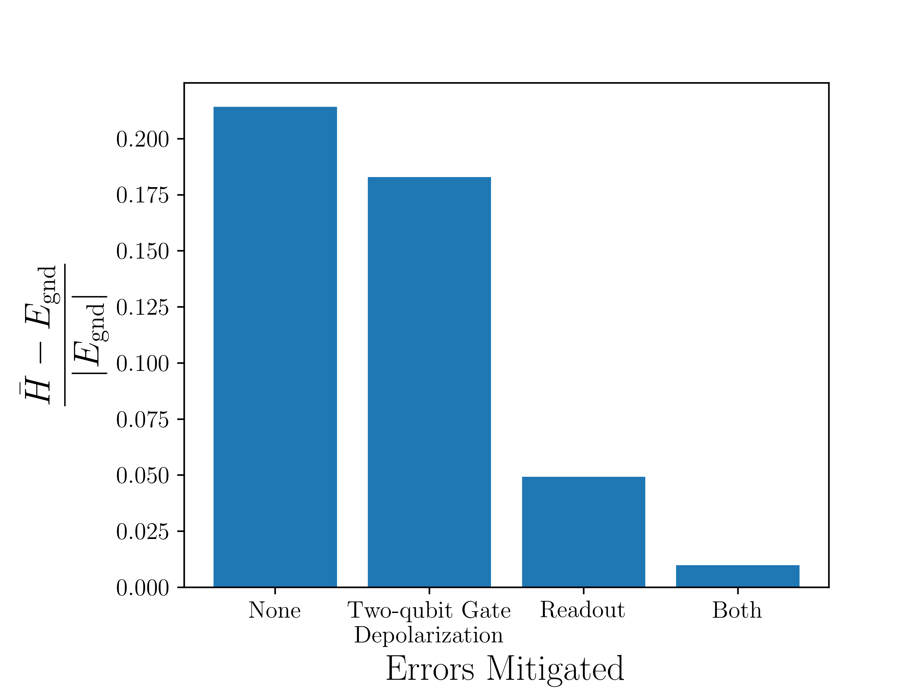
We characterize the improvements to the accuracy in measured average values of the observables obtained by using error mitigation when the variational parameter is fixed at its known optimum value, . First, we test how adding each mitigation technique separately to the process of estimating improves the accuracy. We also mitigate both measurement errors and two-qubit gate errors by applying the inverted calibration matrix to the probability distributions obtained from each of the circuits in Fig. 5; subsequently, results from calculating with each of these circuits can be used to linearly extrapolate a value of with , to mitigate two-qubit gate depolarization errors in addition to readout errors. Results comparing these techniques separately and together for are presented in Fig. 6, where it can be seen that mitigating both the readout and CNOT errors improves the accuracy of the results substantially.
VI Computing observables
To be of interest to experiments, such as direct detection of dark matter, we need to not only be able to compute the energy of an optimal VQE trial for a many-body ground state with lower complexity and greater accuracy than classical computations, but also to use the approximate ground state wave function to compute physical observables. As a stand-in for this goal, we here compute expectation values of observables in the LMG model, such as , , and for , as given by Eqs. (6), (2), and (3), where . In this section, we explore the precision of results obtained from current hardware; specifically, given the availability of readout error mitigation techniques Qiskit Development Team 2020h, we consider results of simulations with a noise model including all sources of infidelity described in Sec. V except for readout error, to compare with exact analytic calculations of the LMG model.
As in the preceding calculations, we consider the system with . In this case, note that for , , so we may summarize the behavior of all moments
| (25) |
for all powers using only the values with a given state . Furthermore, by the symmetries , as per Eq. (9), we can observe that exactly for all values of . Thus, we need to consider only , , and . The fractional deviation of these averages obtained with the VQE optimal value from results obtained with the exact solution are displayed in Fig. 7.

Results obtained here from VQE calculations may be compared to those obtained classically such as in Ref. Fox et al. 2020. For example, their classical calculation of the spin-orbit coupling operator averaged over the ground state carries a fractional deviation of . While the deviation of is significantly smaller in comparison, both and can carry much larger fractional deviations . Even with precise calculations of the ground state energy, useful calculations of the averaged values of spin operators such as and will require reduction in other noise errors such as thermal relaxation of qubits over two-qubit gate operations, as discussed in Sec. V.
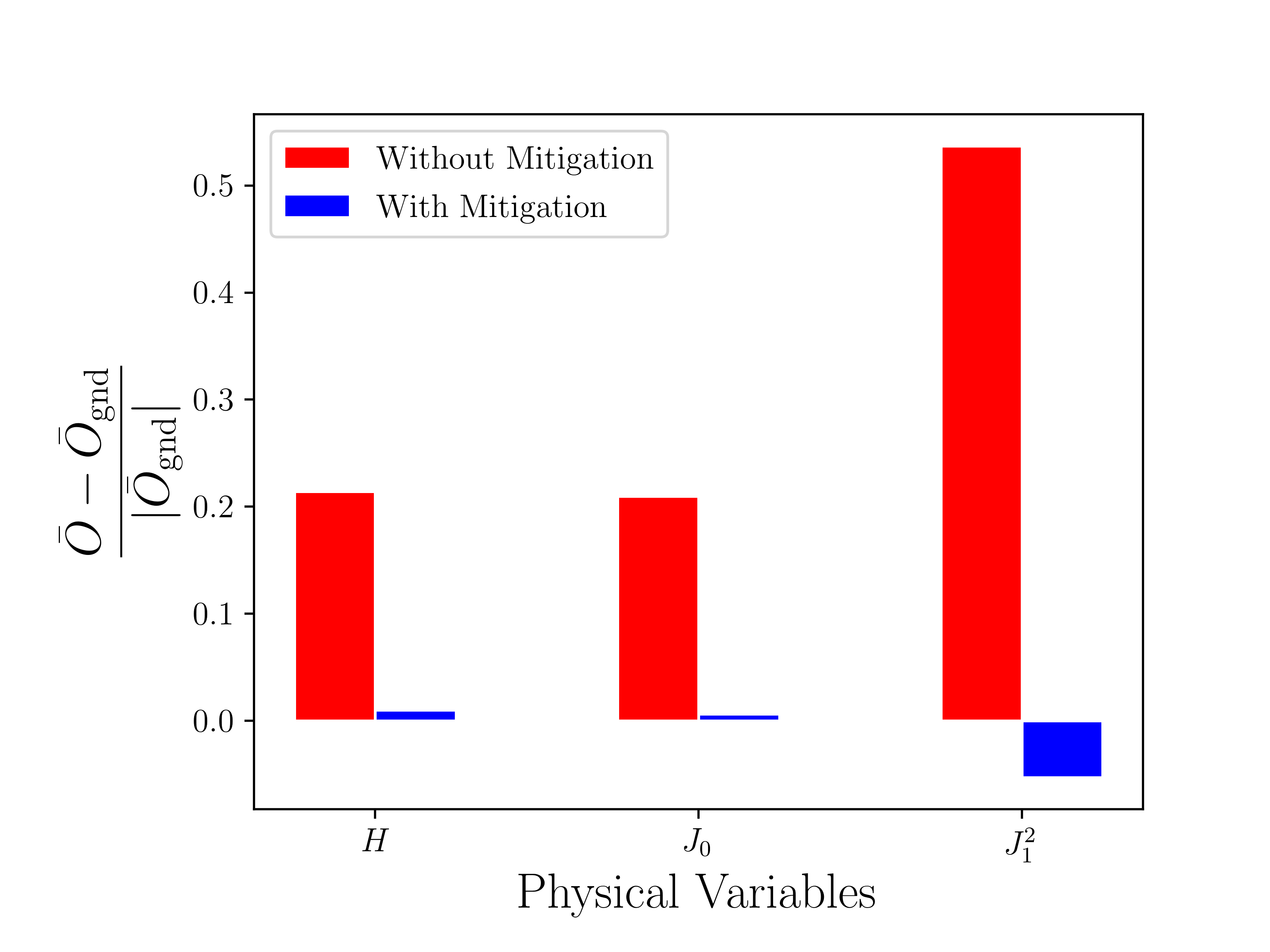
We now characterize the improvements to the accuracy in measured average values of the observables and that are obtained by using error mitigation as described in Sec. V.3. We again measure the observables for the variational state with the known optimum value of the variational parameter for circuits in which the CNOT is replaced by three CNOTs and extrapolate the results back to obtain the error-mitigated result. These results are displayed in Fig. 8. We find that this mitigation technique yields improvements of an order of magnitude in the accuracy of the measured observables and . However, significant additional accuracy improvements will still be needed to exceed the precision of existing classical calculations of these observables in more realistic situations, such as results presented in Ref. Fox et al. 2020.
VII Summary
Appropriate interpretation of the results of experiments, including upper bounds, requires reliable models of target nuclides, including quantified uncertainties. Quantum computing has the potential to enable one to go beyond the limitations of classical calculations, improving the models as well as understanding the uncertainties in those models.
Studying the ground state of many-body systems similar to the LMG model can pose a complex quantum problem. Highly accurate quantum processors are needed for quantum computing to yield improvements over classical algorithms. To identify and assess the most significant sources of error in an existing quantum processor, we develop quantum circuits for VQE calculations on the LMG model and implement the algorithm for the simplest nontrivial case. We compare VQE results and the exact ground state of the LMG model and identify the dominant errors limiting the accuracy of the calculation. We find that readout error and two-qubit gate errors are the dominant sources of infidelities using current quantum hardware. Further, we find that error mitigation techniques improve the accuracy of the calculations substantially. Our results suggest that, given recent rapid advances in the development of quantum computing hardware Satzinger et al. 2021, near-term quantum computers could help with the calculation of at least gross properties of nuclear ground states.
Acknowledgments
The authors acknowledge support by the U.S. Department of Energy, Office of Science, Office of High Energy Physics, under Award No. DE-SC0019465. This work was also supported in part by the National Science Foundation Grant No. PHY-1806368. We thank IBM Quantum Experience for making their quantum processors publicly available.
References
- Blumenthal et al. (1984) G. R. Blumenthal, S. Faber, J. R. Primack, and M. J. Rees, Nature 311, 517 (1984).
- Primack et al. (1988) J. R. Primack, D. Seckel, and B. Sadoulet, Annu. Rev. Nucl. Part. Sci. 38, 751 (1988).
- Feng (2010) J. L. Feng, Ann. Rev. Astron. Astrophys. 48, 495 (2010).
- Bertone and Hooper (2018) G. Bertone and D. Hooper, Rev. Mod. Phys. 90, 045002 (2018).
- Frieman et al. (2008) J. Frieman, M. Turner, and D. Huterer, Ann. Rev. Astron. Astrophys. 46, 385 (2008).
- Dine and Kusenko (2003) M. Dine and A. Kusenko, Rev. Mod. Phys. 76, 1 (2003).
- Kajino et al. (2019) T. Kajino, W. Aoki, A. B. Balantekin, R. Diehl, M. A. Famiano, and G. J. Mathews, Prog. Part. Nucl. Phys. 107, 109 (2019).
- Dolinski et al. (2019) M. J. Dolinski, A. W. P. Poon, and W. Rodejohann, Annu. Rev. Nucl. Part. Sci. 69, 219 (2019).
- Mirizzi et al. (2016) A. Mirizzi, I. Tamborra, H.-T. Janka, N. Saviano, K. Scholberg, R. Bollig, L. Hudepohl, and S. Chakraborty, Riv. Nuovo Cim. 39, 1 (2016).
- Schumann (2019) M. Schumann, J. Phys. G 46, 103003 (2019).
- Cannoni (2013) M. Cannoni, Phys. Rev. D 87, 075014 (2013).
- Cerdeño et al. (2013) D. G. Cerdeño, M. Fornasa, J.-H. Huh, and M. Peiró, Phys. Rev. D 87, 023512 (2013).
- Furnstahl et al. (2015) R. Furnstahl, D. Phillips, and S. Wesolowski, Journal of Physics G: Nuclear and Particle Physics 42, 034028 (2015).
- Carlsson et al. (2016) B. D. Carlsson, A. Ekström, C. Forssén, D. F. Strömberg, G. R. Jansen, O. Lilja, M. Lindby, B. A. Mattsson, and K. A. Wendt, Physical Review X 6, 011019 (2016).
- Pérez et al. (2016) R. N. Pérez, J. Amaro, and E. R. Arriola, International Journal of Modern Physics E 25, 1641009 (2016).
- Yoshida et al. (2018) S. Yoshida, N. Shimizu, T. Togashi, and T. Otsuka, Phys. Rev. C 98, 061301(R) (2018).
- Fox et al. (2020) J. M. R. Fox, C. W. Johnson, and R. N. Perez, Phys. Rev. C 101, 054308 (2020).
- Hempel et al. (2018) C. Hempel, C. Maier, J. Romero, J. McClean, T. Monz, H. Shen, P. Jurcevic, B. P. Lanyon, P. Love, R. Babbush, A. Aspuru-Guzik, R. Blatt, and C. F. Roos, Physical Review X 8, 031022 (2018).
- Cao et al. (2019) Y. Cao, J. Romero, J. P. Olson, M. Degroote, P. D. Johnson, M. Kieferová, I. D. Kivlichan, T. Menke, B. Peropadre, N. P. Sawaya, et al., Chemical reviews 119, 10856 (2019).
- Arute et al. (2020) F. Arute, K. Arya, R. Babbush, D. Bacon, J. C. Bardin, R. Barends, S. Boixo, M. Broughton, B. B. Buckley, D. A. Buell, B. Burkett, N. Bushnell, Y. Chen, Z. Chen, B. Chiaro, R. Collins, W. Courtney, S. Demura, A. Dunsworth, E. Farhi, et al., Science 369, 1084 (2020), https://science.sciencemag.org/content/369/6507/1084.full.pdf .
- Dumitrescu et al. (2018) E. F. Dumitrescu, A. J. McCaskey, G. Hagen, G. R. Jansen, T. D. Morris, T. Papenbrock, R. C. Pooser, D. J. Dean, and P. Lougovski, Physical Review Letters 120, 210501 (2018).
- Roggero et al. (2020) A. Roggero, A. C. Y. Li, J. Carlson, R. Gupta, and G. N. Perdue, Phys. Rev. D 101, 074038 (2020).
- Kreshchuk et al. (2021) M. Kreshchuk, S. Jia, W. M. Kirby, G. Goldstein, J. P. Vary, and P. J. Love, Entropy 23, 597 (2021), arXiv:2009.07885 [quant-ph] .
- Mueller et al. (2020) N. Mueller, A. Tarasov, and R. Venugopalan, Physical Review D 102, 016007 (2020).
- Babbush et al. (2017) R. Babbush, D. W. Berry, Y. R. Sanders, I. D. Kivlichan, A. Scherer, A. Y. Wei, P. J. Love, and A. Aspuru-Guzik, Quantum Science and Technology 3, 015006 (2017).
- Ryabinkin et al. (2018) I. G. Ryabinkin, T.-C. Yen, S. N. Genin, and A. F. Izmaylov, Journal of chemical theory and computation 14, 6317 (2018).
- Romero et al. (2018) J. Romero, R. Babbush, J. R. McClean, C. Hempel, P. J. Love, and A. Aspuru-Guzik, Quantum Science and Technology 4, 014008 (2018).
- Lipkin et al. (1965) H. J. Lipkin, N. Meshkov, and A. J. Glick, Nucl. Phys. 62, 188 (1965).
- Peruzzo et al. (2014) A. Peruzzo, J. McClean, P. Shadbolt, M.-H. Yung, X.-Q. Zhou, P. Love, A. Aspuru-Guzik, and J. L. O’Brien, Nature Communications 5, 4213 (2014).
- Temme et al. (2017) K. Temme, S. Bravyi, and J. M. Gambetta, Physical Review Letters 119, 180509 (2017).
- He et al. (2020) A. He, B. Nachman, W. A. de Jong, and C. W. Bauer, Phys. Rev. A 102, 012426 (2020).
- Bertone et al. (2005) G. Bertone, D. Hooper, and J. Silk, Physics Reports 405, 279 (2005).
- Jungman et al. (1996) G. Jungman, M. Kamionkowski, and K. Griest, Phys. Rep. 267, 195 (1996).
- Sadoulet (1999) B. Sadoulet, Rev. Mod. Phys. 71, S197 (1999).
- Goodman and Witten (1985) M. W. Goodman and E. Witten, Phys. Rev. D 31, 3059 (1985).
- Fitzpatrick et al. (2013) A. Fitzpatrick, W. Haxton, E. Katz, N. Lubbers, and Y. Xu, JCAP 02, 004 (2013).
- Anand et al. (2014) N. Anand, A. L. Fitzpatrick, and W. Haxton, Physical Review C 89, 065501 (2014).
- Vietze et al. (2015) L. Vietze, P. Klos, J. Menéndez, W. Haxton, and A. Schwenk, Phys. Rev. D 91, 043520 (2015).
- Fieguth et al. (2018) A. Fieguth, M. Hoferichter, P. Klos, J. Menéndez, A. Schwenk, and C. Weinheimer, Phys. Rev. D 97, 103532 (2018).
- Hoferichter et al. (2020) M. Hoferichter, J. Menéndez, and A. Schwenk, Phys. Rev. D 102, 074018 (2020).
- Alsum (2020) S. K. Alsum, Effective Field Theory Search Results from the LUX Run 4 Data Set, and Construction of the LZ System Test Platforms, Ph.D. thesis, The University of Wisconsin-Madison (2020).
- Navrátil et al. (2000) P. Navrátil, J. Vary, and B. Barrett, Physical Review C 62, 054311 (2000).
- Barrett et al. (2013) B. R. Barrett, P. Navrátil, and J. P. Vary, Progress in Particle and Nuclear Physics 69, 131 (2013).
- Hagen et al. (2010) G. Hagen, T. Papenbrock, D. J. Dean, and M. Hjorth-Jensen, Physical Review C 82, 034330 (2010).
- Brussard and Glaudemans (1977) P. J. Brussard and P. W. M. Glaudemans, Shell-Model Applications in Nuclear Spectroscopy (North-Holland Publishing Company, Amsterdam, 1977).
- Brown and Wildenthal (1988) B. A. Brown and B. H. Wildenthal, Annu. Rev. Nuc. Part. Sci. 38, 29 (1988).
- Caurier et al. (2005) E. Caurier, G. Martinez-Pinedo, F. Nowacki, A. Poves, and A. P. Zuker, Rev. Mod. Phys. 77, 427 (2005).
- Stroberg et al. (2019) S. R. Stroberg, H. Hergert, S. K. Bogner, and J. D. Holt, Annu. Rev. Nuc. Part. Sci. 69, 307 (2019).
- Pacheco and Strottman (1989) A. F. Pacheco and D. Strottman, Phys. Rev. D 40, 2131 (1989).
- Ressell et al. (1993) M. T. Ressell, M. B. Aufderheide, S. D. Bloom, K. Griest, G. J. Mathews, and D. A. Resler, Phys. Rev. D 48, 5519 (1993).
- Pirinen et al. (2016) P. Pirinen, P. C. Srivastava, J. Suhonen, and M. Kortelainen, Phys. Rev. D 93, 095012 (2016).
- Menéndez et al. (2012) J. Menéndez, D. Gazit, and A. Schwenk, Phys. Rev. D 86, 103511 (2012).
- Klos et al. (2013) P. Klos, J. Menéndez, D. Gazit, and A. Schwenk, Phys. Rev. D 88, 083516 (2013).
- Baudis et al. (2013) L. Baudis, G. Kessler, P. Klos, R. F. Lang, J. Menéndez, S. Reichard, and A. Schwenk, Phys. Rev. D 88, 115014 (2013).
- Gazda et al. (2017) D. Gazda, R. Catena, and C. Forssén, Phys. Rev. D 95, 103011 (2017).
- Hoferichter et al. (2019) M. Hoferichter, P. Klos, J. Menéndez, and A. Schwenk, Phys. Rev. D 99, 055031 (2019).
- Lloyd (1996) S. Lloyd, Science 273, 1073 (1996).
- Clemente et al. (2020) G. Clemente, M. Cardinali, C. Bonati, E. Calore, L. Cosmai, M. D’Elia, A. Gabbana, D. Rossini, F. S. Schifano, R. Tripiccione, and D. Vadacchino (QuBiPF Collaboration), Phys. Rev. D 101, 074510 (2020).
- Loh et al. (1990) E. Y. Loh, Jr., J. E. Gubernatis, R. T. Scalettar, S. R. White, D. J. Scalapino, and R. L. Sugar, Physical Review B 41, 9301 (1990).
- Krieger (1977) S. Krieger, Nuclear Physics A 276, 12 (1977).
- Hoodbhoy and Negele (1978) P. Hoodbhoy and J. W. Negele, Phys. Rev. C 18, 2380 (1978).
- Wahlen-Strothman et al. (2017) J. M. Wahlen-Strothman, T. M. Henderson, M. R. Hermes, M. Degroote, Y. Qiu, J. Zhao, J. Dukelsky, and G. E. Scuseria, The Journal of Chemical Physics 146, 054110 (2017).
- Stoica et al. (2001) S. Stoica, I. Mihut, and J. Suhonen, Phys. Rev. C 64, 017303 (2001).
- Severyukhin et al. (2006) A. P. Severyukhin, M. Bender, and P.-H. Heenen, Phys. Rev. C 74, 024311 (2006).
- Lacroix (2009) D. Lacroix, Phys. Rev. C 79, 014301 (2009).
- Bertolli and Papenbrock (2008) M. G. Bertolli and T. Papenbrock, Phys. Rev. C 78, 064310 (2008).
- Plesch and Brukner (2011) M. Plesch and C. Brukner, Phys. Rev. A 83, 032302 (2011).
- Ortiz et al. (2005) G. Ortiz, R. Somma, J. Dukelsky, and S. Rombouts, Nuclear Physics B 707, 421 (2005).
- Lerma H. and Dukelsky (2013) S. Lerma H. and J. Dukelsky, Nucl. Phys. B870, 421 (2013).
- Somma (2005) R. D. Somma, Quantum computation, complexity, and many-body physics, Ph.D. thesis (2005), Ph.D. Thesis.
- (71) K. Robbins and P. J. Love, arXiv:2105.06761 .
- Rubio et al. (2019) J. Rubio, D. Bevenius, O. Costa Hamido, J. Carballo, A. Rodríguez Davila, J. Cruz-Benito, and W. Hu, “Qiskit (Quantum Information Science Kit) for JavaScript,” (2019).
- Qiskit Development Team (2020a) Qiskit Development Team, “IBM Quantum Experience glossary,” https://quantum-computing.ibm.com/docs/glossary/ (2020a), accessed: 2020-10-08.
- IBM Quantum (2020) IBM Quantum, “IBM Quantum Experience Open QASM Simulator,” https://quantum-computing.ibm.com/docs/manage/backends/simulators/ (2020), accessed: 2020-10-08.
- Qiskit Development Team (2020b) Qiskit Development Team, “Qiskit: Device backend noise model simulations,” https://qiskit.org/documentation/tutorials/simulators/2_device_noise_simulation.html (2020b), accessed: 2020-10-09.
- Qiskit Development Team (2020c) Qiskit Development Team, “Qiskit: Readouterror,” https://qiskit.org/documentation/stubs/qiskit.providers.aer.noise.ReadoutError.html (2020c), accessed: 2020-10-09.
- Qiskit Development Team (2020d) Qiskit Development Team, “Qiskit: Ibmqbackend.properties,” https://qiskit.org/documentation/stubs/qiskit.providers.ibmq.IBMQBackend.properties.html (2020d), accessed: 2020-10-09.
- Qiskit Development Team (2020e) Qiskit Development Team, “Qiskit: U1gate,” https://qiskit.org/documentation/stubs/qiskit.circuit.library.U1Gate.html (2020e), accessed: 2020-10-27.
- Qiskit Development Team (2020f) Qiskit Development Team, “Qiskit: U3gate,” https://qiskit.org/documentation/stubs/qiskit.circuit.library.U3Gate.html (2020f), accessed: 2020-10-27.
- Nation (2020) P. Nation, “Randomized benchmarking,” https://github.com/Qiskit/qiskit-tutorials/blob/master/tutorials/noise/4_randomized_benchmarking.ipynb (2020).
- Qiskit Development Team (2020g) Qiskit Development Team, “Qiskit: Noise models,” https://qiskit.org/documentation/apidoc/aer_noise.html (2020g), accessed: 2020-10-09.
- Qiskit Development Team (2020h) Qiskit Development Team, “Qiskit: Measurement error mitigation,” https://qiskit.org/textbook/ch-quantum-hardware/measurement-error-mitigation.html (2020h), accessed: 2020-10-09.
- Satzinger et al. (2021) K. J. Satzinger, Y. Liu, A. Smith, C. Knapp, M. Newman, C. Jones, Z. Chen, C. Quintana, X. Mi, A. Dunsworth, C. Gidney, I. Aleiner, F. Arute, K. Arya, J. Atalaya, R. Babbush, J. C. Bardin, R. Barends, J. Basso, A. Bengtsson, et al., “Realizing topologically ordered states on a quantum processor,” (2021), arXiv:2104.01180 [quant-ph] .