跳到论文正文
W Papers独立论文阅读器 arXiv:2011.03791 论文正文 计算阅读时间 · 0%
引用这篇论文根据当前论文元数据生成,正式投稿前建议核对。


License: arXiv.org perpetual non-exclusive license
arXiv:2011.03791v3 [cs.GT] 19 Jul 2021

How Likely Are Large Elections Tied?

Lirong Xia    Rensselaer Polytechnic Institute    Troy    NY 12180    USA Email: xialirong@gmail.com
Abstract

Understanding the likelihood for an election to be tied is a classical topic in many disciplines including social choice, game theory, political science, and public choice. The problem is important not only as a fundamental problem in probability theory and statistics, but also because it plays a critical role in many other important issues such as indecisiveness of voting, strategic voting, privacy of voting, voting power, voter turnout, etc. Despite a large body of literature and the common belief that ties are rare, little is known about how rare ties are in large elections except for a few simple positional scoring rules under the i.i.d. uniform distribution over the votes, known as the Impartial Culture (IC) in social choice. In particular, little progress was made after Marchant explicitly posed the likelihood of kk-way ties under IC as an open question in 2001 [39].

We give an asymptotic answer to this open question for a wide range of commonly studied voting rules under a more general and realistic model, called the smoothed social choice framework [67], which was inspired by the celebrated smoothed complexity analysis Spielman and Teng 2009. We prove dichotomy theorems on the smoothed likelihood of ties under positional scoring rules, edge-order-based rules, and some multi-round score-based elimination rules, which include commonly studied voting rules such as plurality, Borda, veto, maximin, Copeland, ranked pairs, Schulze, STV, and Coombs as special cases. We also complement the theoretical results by experiments on synthetic data and real-world rank data on Preflib [42]. Our main technical tool is an improved characterization of the smoothed likelihood for a Poisson multinomial variable to be in a polyhedron, by exploring the interplay between the V-representation and the matrix representation of polyhedra and might be of independent interest.

1 Introduction

Suppose a presidential election between two alternatives (candidates) aa and bb will be held soon, and there are nn agents (voters). Each agent independently votes for an alternative with probability 0.50.5, and the alternative with more votes wins. How likely will the election end up with a tie? What if there are more than two alternatives, agents rank the alternatives, and a rank-based voting rule is used to choose the winner? What if the distribution is not independent and identically distributed (i.i.d.) and is controlled by an adversary?

Understanding the likelihood of tied elections is an important and classical topic in many disciplines including social choice, game theory, political science, and public choice, not only because it is a fundamental problem in probability theory and statistics, but also because it plays a critical role in many important issues. For example, ties are undesirable in the context of indecisiveness of voting [28], strategic voting [27, 57], privacy of voting [36], etc. On the other hand, ties are desirable in the context of voting power [4], voter turnout [20, 56], etc.

While the likelihood of ties for two alternatives is well-understood [4, 6], we are not aware of a rigorous mathematical analysis for elections with three or more alternatives except for a few simple voting rules. Previous studies were mostly done along three dimensions: (1) the voting rule used in the election, (2) the indecisiveness of the outcome, measured by the number of tied alternatives kk, and (3) the statistical model for generating votes. See Section 1.1 for more discussions.

Despite these efforts, the following question largely remains open.

How likely are large elections tied under realistic models?

Specifically, Marchant [39] posed the likelihood of ties beyond certain positional scoring rules under the i.i.d. uniform distribution, known as the Impartial Culture (IC) in social choice, as an open question in 2001, but we are not aware of any progress afterwards. While IC has been a popular choice in social choice theory, it has also been widely criticized of being unrealistic [35].

In fact, the question is already highly challenging under IC as illustrated in Example 1 below. Consider the probability of 33-way ties under the Borda rule for 33 alternatives and nn agents. Borda is a positional scoring rule, which scores every alternative according to its rank. Under Borda, each agent uses a linear order over the alternatives to represent his/her preferences, and the ii-th ranked alternative gets m−im-i points. The winners are the alternatives with maximum total points.

Example 1.

Let 𝒜={1,2,3}\mathcal{A}=\{1,2,3\} denote the set of alternatives. For each linear order RR over 𝒜\mathcal{A}, let XRX_{R} denote the random variable that represents the number of agents whose votes are RR, when their votes are generated uniformly at random (i.e., IC). For example, X123X_{123} represents the multiplicity of 1≻2≻31\succ 2\succ 3. Then, the probability of 33-way ties under Borda w.r.t. IC can be represented by the probability for the following system of linear equations to hold, where (1) states that alternatives 11 and 22 are tied, (2) states that 22 and 33 are tied, and (3) states that 11 and 33 are tied.

2​X123+2​X132+X213+X312=2​X213+2​X231+X123+X321\displaystyle 2X_{123}+2X_{132}+X_{213}+X_{312}=2X_{213}+2X_{231}+X_{123}+X_{321} (1)
2​X213+2​X231+X123+X321=2​X312+2​X321+X132+X231\displaystyle 2X_{213}+2X_{231}+X_{123}+X_{321}=2X_{312}+2X_{321}+X_{132}+X_{231} (2)
2​X123+2​X132+X213+X312=2​X312+2​X321+X132+X231\displaystyle 2X_{123}+2X_{132}+X_{213}+X_{312}=2X_{312}+2X_{321}+X_{132}+X_{231} (3)

The difficulty in accurately bounding the likelihood of ties comes from two types of statistical correlations. The first type consists of correlations among components of XX. That is, for any pairs of linear orders RR and WW, XRX_{R} and XWX_{W} are statistically dependent. The second type consists of correlations among equations, and more generally, inequalities as we will see in the general problem studied in this paper. For example, while it is straightforward to see that (1) and (2) implies (3) in Example 1, it is unclear how much correlation exists between (1) and (2). Existing asymptotic tools such as multivariate Central Limit Theorems and Berry-Esseen-type Theorems [7, 62, 17, 18, 55] (a.k.a. Lyapunov-type bounds) contain an O⁡(n−0.5)O(n^{-0.5}) or higher error bound, which are too coarse and do not match the lower bound that will be proved in this paper. The problem becomes more challenging for inequalities, other voting rules, other number of alternatives, other kk’s, and non-i.i.d. distributions over votes.

The Model.

We address the likelihood of ties under the smoothed social choice framework [67], which is inspired by the celebrated smoothed complexity analysis [60]. We believe that the framework is more general and realistic than the extensively studied i.i.d. models, especially IC. In the framework, agents’ “ground truth” preferences can be arbitrarily correlated and are chosen by an adversary, and then independent noises are added to form their votes. Mathematically, the adversary chooses a distribution πj\pi_{j} for each agent jj from a set Π\Pi of distributions over all linear orders over the alternatives, under which the probability of various events of interest are studied, for example Condorcet’s paradox and satisfaction of axioms [67].

Our Contributions.

In this paper, we adopt the statistical model in [67] to formulate and study the smoothed likelihood of ties. Given an (irresolute) voting rule rr, 2≤k≤m2\leq k\leq m, and n∈ℕn\in\mathbb{N} agents, the max-adversary aims to maximize the likelihood of kk-way ties, denoted by Tie~Πmax​(r,k,n)\widetilde{\text{Tie}}^{\max}_{\Pi}(r,k,n), by choosing π→=(π1,…,πn)∈Πn\vec{\pi}=(\pi_{1},\ldots,\pi_{n})\in\Pi^{n}. Formally,

Tie~Πmax​(r,k,n)≜supπ→∈ΠnPrP∼π→⁡(|r⁡(P)|=k)\widetilde{\text{Tie}}^{\max}_{\Pi}(r,k,n)\triangleq\sup\nolimits_{\vec{\pi}\in\Pi^{n}}\Pr\nolimits_{P\sim\vec{\pi}}\left(|r(P)|=k\right) (4)

Similarly, the min-adversary aims to minimize the likelihood of kk-way ties defined as follows:

Tie~Πmin​(r,k,n)≜infπ→∈ΠnPrP∼π→⁡(|r⁡(P)|=k)\widetilde{\text{Tie}}^{\min}_{\Pi}(r,k,n)\triangleq\inf\nolimits_{\vec{\pi}\in\Pi^{n}}\Pr\nolimits_{P\sim\vec{\pi}}\left(|r(P)|=k\right) (5)

We call Tie~Πmax​(r,k,n)\widetilde{\text{Tie}}^{\max}_{\Pi}(r,k,n) (respectively, Tie~Πmin​(r,k,n)\widetilde{\text{Tie}}^{\min}_{\Pi}(r,k,n)) the max (respectively, min) smoothed likelihood of ties. When Π\Pi consists of a single distribution π\pi, Tie~Πmax​(r,k,n)\widetilde{\text{Tie}}^{\max}_{\Pi}(r,k,n) and Tie~Πmin​(r,k,n)\widetilde{\text{Tie}}^{\min}_{\Pi}(r,k,n) coincide with each other and become the likelihood of ties under i.i.d. distribution π\pi. In particular, when Π={πuni}\Pi=\{\pi_{\text{uni}}\}, where πuni\pi_{\text{uni}} is the uniform distribution, Tie~Πmax​(r,k,n)\widetilde{\text{Tie}}^{\max}_{\Pi}(r,k,n) and Tie~Πmin​(r,k,n)\widetilde{\text{Tie}}^{\min}_{\Pi}(r,k,n) become the classical analysis of ties under IC. As discussed in [67], the smoothed social choice framework allows agents’ ground truth preferences to be arbitrarily correlated, while the noises are independent, which is a standard assumption in many literatures such as behavior science, economics, statistics, and smoothed complexity analysis.

Our main technical results are asymptotic characterizations of the smoothed likelihood of ties for a fixed number of at least three alternatives (m≥3m\geq 3) in large elections (n→∞n\rightarrow\infty). Informally, our main results can be summarized as follows.

Main results: smoothed likelihood of ties, informally put. Under mild assumptions on Π\Pi, for many commonly studied voting rules rr, for any fixed m≥3m\geq 3, any 2≤k≤m2\leq k\leq m, and any n∈ℕn\in\mathbb{N}, Tie~Πmax​(r,k,n)\widetilde{\text{Tie}}^{\max}_{\Pi}(r,k,n) (respectively, Tie~Πmin​(rs→,k,n)\widetilde{\text{Tie}}^{\min}_{\Pi}(r_{\vec{s}},k,n)) is either 00, exp⁡(−Θ⁡(n))\exp(-\Theta(n)), or Θ​(poly−1​(n))\Theta(\text{poly}^{-1}(n)).

More precisely, we prove Theorem 3 for integer positional scoring rules (including plurality, Borda, veto), Theorem 4 for edge-order-based rules (including maximin, Schulze, ranked pairs, and Copeland, see Definition 11), and Theorem 5 for STV and Coombs. The formal statements of the theorems also characterize the condition for each (00, exponential, or polynomial) case as well as asymptotically tight bounds in the polynomial cases.

When ties are undesirable, e.g., in the context of indecisiveness of voting, strategic voting, or privacy, a low max smoothed likelihood is good news. When ties are desirable, e.g., in the context of voting power and voter turnout, a high min smoothed likelihood is good news. Our theorems therefore completely characterize conditions for good news in different contexts.

Straightforward applications of our theorems answer the open question by Marchant [39] for many commonly studied voting rules as summarized in Table 1 below.

Table 1: Probability of kk-way ties (2≤k≤m2\leq k\leq m) under some commonly studied voting rules w.r.t. IC. For Copelandα, lαl_{\alpha} is the minimum positive integer s.t. α​lα∈ℤ\alpha l_{\alpha}\in\mathbb{Z}.
Int. Pos. scoring (Coro. 1)
STV and Coombs (Prop. 6)
maximin (Prop. 3)
Schulze (Prop. 4)
ranked pairs (Prop. 5)
{0nkΘ⁡(n−k−12)otherwise\left\{\begin{array}[]{@{}l l@{}}0&\text{\begin{tabular}[]{@{}l}if no profile of $n$ votes\\ contains a $k$-way tie\end{tabular}}\\ \Theta(n^{-\frac{k-1}{2}})&\text{otherwise}\end{array}\right.
Θ⁡(n−k−12)\Theta(n^{-\frac{k-1}{2}})
Lower Upper
{Ω(n−k−12)Ω(n−⌈log⁡k⌉2)m≥k+5⌈logk⌉\left\{\text{\begin{tabular}[]{@{}l@{}}$\Omega(n^{-\frac{k-1}{2}})$\\ $\Omega(n^{-\frac{\lceil\log k\rceil}{2}})$ if $m\geq k+5\lceil\log k\rceil$\end{tabular}}\right. n−Ω⁡(log⁡klog⁡log⁡k)n^{-\Omega(\frac{\log k}{\log\log k})}
Copelandα (𝟎≤α≤𝟏0\leq\alpha\leq 1) (Prop. 2)
{0if ​2∤n,2|k,and ​k≥m−1Θ⁡(n−k4)if ​2|n,2|k,a​n​d​{(1)​k=m, or(2)​k=m−1​ and ​α≥12, or(3)​k=m−1​ and ​k≤lα​(lα+1)Θ⁡(n−lα​(lα+1)4)if ​2|n,2|k,k=m−1,α⁡<12, and ​k>​lα​(lα+1)Θ⁡(1)otherwise (i.e., if ​2∤k​ or ​k≤m−2​)\left\{\begin{array}[]{ll}0&\text{if }2\nmid n,2\mid k,\text{and }k\geq m-1\\ \Theta(n^{-\frac{k}{4}})&\text{if }2\mid n,2\mid k,{and}\left\{\begin{array}[]{l}(1)\ k=m,\text{ or}\\ (2)\ k=m-1\text{ and }\alpha\geq\frac{1}{2},\text{ or}\\ (3)\ k=m-1\text{ and }k\leq l_{\alpha}(l_{\alpha}+1)\end{array}\right.\\ \Theta\left(n^{-\frac{l_{\alpha}(l_{\alpha}+1)}{4}}\right)&\text{if }2\mid n,2\mid k,k=m-1,\alpha<\frac{1}{2},\text{ and }k>l_{\alpha}(l_{\alpha}+1)\\ \Theta(1)&\text{otherwise (i.e., if }2\nmid k\text{ or }k\leq m-2\text{)}\end{array}\right.

Roughly speaking, Table 1 reveals the following ranking over the voting rules w.r.t. their likelihood of kk-way ties under IC, for every 2≤k≤m2\leq k\leq m.

{Int. Pos. Scoring, STV, Coombs}≤{maximin, Schulze}≤ranked pairs≤Copeland\{\text{Int. Pos. Scoring, STV, Coombs}\}\leq\{\text{maximin, Schulze}\}\leq\text{ranked pairs}\leq\text{Copeland}

A closely related question is the likelihood of any-way ties, sometimes referred to as indecisiveness [39], under IC, i.e., the election admits a kk-way tie for any 2≤k≤m2\leq k\leq m. It is not hard to see from Table 1 that such likelihood is dominated by the probability of 22-way ties and is either 00 or Θ⁡(1n)\Theta(\frac{1}{\sqrt{n}}) for all rules in the table except ranked pairs and Copeland, which are covered by Proposition 5 and Proposition 2, respectively. To the best of our knowledge, these results are new, except for plurality and Borda. Experiments on synthetic data generated from IC confirm these observations, while experiments on Preflib data [42] reveal a difference order, where ties are rare under Borda (1.6%) and Copeland (2.6%), and are quite common under veto (31.3%) due to situations where m>nm>n.

Technical Innovations.

The proofs of the smoothed likelihood of ties in this paper follow the same high-level idea. We first model the existence of a kk-way tie by systems of linear inequalities that are similar to the ones in Example 1. In this way, the likelihood of ties becomes the likelihood for the histogram of the randomly generated profile, which is a Poisson multivariate variable (PMV), to be in the polyhedron ℋ{\mathcal{H}} represented by the linear inequalities. Then, we prove a dichotomous characterization (Theorem 1) for a PMV to be in ℋ{\mathcal{H}}, and finally apply Theorem 1 (more precisely, its extension Theorem 2 to unions of multiple polyhedra) to characterize the smoothed likelihood of ties.

More precisely, given n,q∈ℕn,q\in\mathbb{N} and a vector π→=(π1,…,πn)\vec{\pi}=(\pi_{1},\ldots,\pi_{n}) of nn distributions over {1,…,q}\{1,\ldots,q\}, an (n,q)(n,q)-PMV is denoted by X→π→{\vec{X}}_{\vec{\pi}}, which represents the histogram of nn independent random variables whose distributions are {π1,…,πn}\{\pi_{1},\ldots,\pi_{n}\}, respectively.

Theorem 1. (The PMV-in-polyhedron theorem, informally put). Let ℋ{\mathcal{H}} denote a polyhedron and Π\Pi denote a set of distributions that satisfy some mild conditions, for any n∈ℕn\in\mathbb{N},

supπ→∈ΠnPr⁡(X→π→∈ℋ)\sup_{\vec{\pi}\in\Pi^{n}}\Pr({\vec{X}}_{\vec{\pi}}\in{\mathcal{H}}) is 00, exp⁡(−Θ⁡(n))\exp(-\Theta(n)), or Θ​(poly​(n))\Theta(\text{poly}(n)), and
infπ→∈ΠnPr⁡(X→π→∈ℋ)\inf_{\vec{\pi}\in\Pi^{n}}\Pr({\vec{X}}_{\vec{\pi}}\in{\mathcal{H}}) is 00, exp⁡(−Θ⁡(n))\exp(-\Theta(n)), or Θ​(poly​(n))\Theta(\text{poly}(n))

The bounds are asymptotically tight and the formal statement of the theorem also characterizes conditions for the 00, exponential, and polynomial cases, respectively. As commented after Example 1, we do not see a way to prove Theorem 1 by straightforward applications of existing asymptotic tools. We also believe that Theorem 1 is a useful tool to study the smoothed likelihood of many events of interest in social choice as commented in [67].

1.1 Related Work and Discussions

Ties in elections. The importance of estimating likelihood of ties has been widely acknowledged, for example, as Mulligan and Hunter commented: “Perhaps it is common knowledge that civic elections are not often decided by one vote…a precise calculation of the frequency of a pivotal vote can contribute to our understanding of how many, if any, votes might be rationally and instrumentally cast” [48]. In practice, however, ties are not as rare as commonly believed, even in high-stakes elections, and have led to pitfalls and consequent modifications of electoral systems and constitutional laws. For example, in the 1800 US presidential election, Jefferson and Burr tied in the electoral college votes. By the Constitution, the House of Representatives should vote until a candidate wins the majority. However, in the subsequent 35 rounds of deadlocked voting, none of the two candidates got the majority. Eventually, Jefferson won the 36th revote to become the president. This “had demonstrated a fundamental flaw with the Constitution. As a result, the Twelfth Amendment to the Constitution was introduced and ratified” [10].

Three-or-more-way ties.

Nowadays, legislators are well-aware of the possibility of two-way ties in elections and have specified tie-breaking mechanisms to handle them. However, three-or-more-way ties have not received their deserved attention and are sometimes overlooked. For example, the 2019 Code of Alabama Section 17-12-23 states: “In all elections where there is a tie between the two highest candidates for the same office, for all county or precinct offices, it shall be decided by lot by the sheriff of the county in the presence of the candidates”. The Code does not specify what action should be taken when three or more candidates are tied for the first place. Results in this paper characterize how rare this happens, so that the legislators can make an informed decision about whether the loophole is a significant concern in practice, and in case it is, how to fix it.

Smoothed analysis.

There is a large body of literature on the applications of smoothed analysis to mathematical programming, machine learning, numerical analysis, discrete math, combinatorial optimization, etc., see [60] for a survey. Smoothed analysis has also been applied to various problems in economics, for example price of anarchy [12] and market equilibrium [33]. In a recent position paper, Baumeister, Hogrebe, and Rothe [5] proposed a Mallows-based model to conduct smoothed analysis on computational aspects of social choice and commented that the model can be used to analyze voting paradoxes and ties, but the paper does not contain technical results. [67] independently proposed to conduct smoothed analysis for paradoxes and impossibility theorems in social choice, characterized the smoothed likelihood of Condorcet’s voting paradox and the ANR impossibility theorem, and proposed a new tie-breaking mechanism. We only use the probabilistic model in [67] and topic-wise, our paper is different from [67], because we formulate and study the smoothed likelihood of ties under commonly studied voting rules, which was not studied in [67].

Technical novelty.

We believe that the main technical tool of this paper (Theorem 1) is a significant and non-trivial extension of Lemma 1 in [67] to arbitrary polyhedron represented by an integer matrix, every nn, and the min-adversary. More discussions can be found in the remark after Theorem 1. We believe that Theorem 1 is a useful tool to analyze smoothed likelihood of many other problems of interest in social choice. For example, all results in [67] can be immediately strengthened by Theorem 1.

Previous work on likelihood of ties.

The following table summarizes previous works that are closest to this paper, whose main contributions are characterizations of likelihood of ties.

Paper 𝒎\bm{m} 𝒌\bm{k} Voting rule Distribution
[6] 22 22 majority two groups, i.i.d. within each group
[40]
[11]
22 22 majority i.i.d. w.r.t. an uncertain distribution
[28] any m∈ℕm\in\mathbb{N} 2≤k≤m2\leq k\leq m plurality uniformly i.i.d. (IC)
[29] 33 2≤k≤m2\leq k\leq m Borda uniformly i.i.d. (IC)
[39] any m∈ℕm\in\mathbb{N} k=mk=m certain scoring rules uniformly i.i.d. over all score vectors

More precisely, Beck [6] studied the probability of ties under the majority rule (over two alternatives) with two groups of agents, whose votes are i.i.d. within each group. Margolis [40] and Chamberlain and Rothschild [11] focused on the majority rule for two alternatives, where agents’ preferences are i.i.d. according to a randomly generated distribution. Gillett [28] studied probability of all-way ties (i.e., k=mk=m) under plurality w.r.t. IC for arbitrary numbers of alternatives and agents. Gillett [29] obtained a closed-form formula for Borda indecisiveness (two or more alternatives being tied) for m=3m=3 w.r.t. IC. Marchant [39] considered a class of scoring rules where each agent can choose a score vector from a given scoring vectors set (SVS), and characterized the asymptotic probability of mm-way ties under a class of scoring rule to be Θ⁡(n1−m2)\Theta(n^{\frac{1-m}{2}}) w.r.t. the i.i.d. uniform distribution over all SVS. This result can be applied to Borda and approval voting but cannot be applied to plurality. Marchant [39] also noted that Domb [19] obtained equivalent formulas for m=3m=3 under Borda. As discussed earlier, the smoothed social choice framework used in our paper is more general. In particular, corollaries of our theorems answer the open questions proposed by Marchant [39] and reveal a ranking over these rules according to the likelihood of ties under IC as summarized in Table 1.

Previous work related to likelihood of ties.

[34] studied the setting where the agents are partitioned into multiple groups, and within each group, agents’ votes are generated from the impartial anonymous culture (IAC) model. The smoothed social choice framework and IAC are not directly comparable. The former is more general in the sense that agents’ “ground truth” preferences are arbitrarily correlated. The latter is more general in the sense that agents’ “noises” are not independent. There is also a line of empirical and mixed empirical-theoretical work on the likelihood of ties under the US electoral college system [25, 26]. Studying the smoothed likelihood of ties under these settings are left for future work.

The probability of tied elections is closely related to the probability for a single voter to be pivotal, sometimes called voting power, which plays an important role in the paradox of voting [20] and in definitions of power indices in cooperative game theory. There is a large body of work on voting games, where the probability for a voter to be pivotal, which is equivalent to the likelihood of ties among other voters, plays a central role in the analysis of voters’ strategic behavior. Examples include seminal works [2, 22, 49], and more recent work [50]. It is not hard to see that the voting power for two alternatives or for multiple alternatives under the plurality rule almost equals to the probability of tied elections with one less vote under certain tie-breaking rules, as pointed out in [30]. For three or more alternatives the two problems are closely related but technically different, which we leave for future work.

The likelihood of ties is also related to the manipulability of voting rules [15]—if an election is not tied, then no single agent can change the outcome, therefore no agent alone has incentive to cast a manipulative vote. Our results are related to but different from the typical-case analysis of manipulability in the literature [54, 68, 46, 66] and the quantitative Gibbard-Satterthwaite theorem [24, 47], where votes are assumed to be i.i.d. Likelihood of ties are also related to but different from the margin of victory [38, 65] and more broadly, bribery and control in elections [21].

Adding noise to study ties.

We are not aware of a previous work that characterized the smoothed likelihood of ties as we do in this paper. The idea of adding noise to study ties is not new. In the definition of resolvability in [61], an additional vote is added to break ties. In [23], irresolute voting rules were defined by taking the union of winners under profiles around a given profile. Another resolvability studied in the literature (see e.g., Formulation#1 in Section 4.2 of [59]11 1 Wikipedia [64] contributes this definition to Douglas R. Woodall but we were not able to find a formal reference.) requires that the probability of ties goes to 00 under the voting rule w.r.t. IC, which is closely related to the literature in the indecisiveness of voting. Our setting and results are more general because IC is a special case of the smoothed social choice framework, and our results also characterize the rate of convergence.

Computational aspects of tie-breaking.

There is a large body of recent work on computational aspects of tie-breaking. [14] proposed the parallel universe tie-breaking (PUT) for multi-stage voting rules and characterized the complexity of the STV rule. [8] characterize the complexity of PUT under ranked pairs, whose smoothed likelihood of ties is studied in this paper. [41] characterized complexity of PUT under other multi-stage voting rules such as Baldwin and Coombs. [52, 51, 3, 53] investigated the effect of different tie-breaking mechanisms to the complexity of manipulation. [23] propose a general way of defining ties under generalized scoring rules. [63] proposed practical AI algorithms for computing PUT under STV and ranked pairs.

2 Preliminaries

Basic Setting. For any q∈ℕq\in\mathbb{N}, we let [q]={1,…,q}[q]=\{1,\ldots,q\}. Let 𝒜=[m]\mathcal{A}=[m] denote the set of m≥3m\geq 3 alternatives. Let ℒ⁡(𝒜)\mathcal{L}(\mathcal{A}) denote the set of all linear orders over 𝒜\mathcal{A}. Let n∈ℕn\in\mathbb{N} denote the number of agents. Each agent uses a linear order to represent his or her preferences, called a vote. The vector of nn agents’ votes, denoted by PP, is called a (preference) profile, sometimes called an nn-profile. A fractional profile is a preference profile PP together with a possibly non-integer and possibly negative weight vector ω→P=(ωR:R∈P)∈ℝn\vec{\omega}_{P}=(\omega_{R}:R\in P)\in{\mathbb{R}}^{n} for the votes in PP. It follows that a non-fractional profile is a fractional profile with uniform weight, namely ω→P=1→\vec{\omega}_{P}=\vec{1}. Sometimes we slightly abuse the notation by omitting the weight vector when it is clear from the context or when ω→P=1→\vec{\omega}_{P}=\vec{1}.

For any (fractional) profile PP, let Hist​(P)∈ℤ≥0m!\text{Hist}(P)\in{\mathbb{Z}}_{\geq 0}^{m!} denote the anonymized profile of PP, also called the histogram of PP, which contains the total weight of every linear order in ℒ⁡(𝒜)\mathcal{L}(\mathcal{A}) according to PP. An (irresolute) voting rule rr is a mapping from a profile to a non-empty set of winners in 𝒜\mathcal{A}. Below we recall the definitions of several commonly studied voting rules.

Integer positional scoring rules.

An (integer) positional scoring rule is characterized by an integer scoring vector s→=(s1,…,sm)∈ℤm\vec{s}=(s_{1},\ldots,s_{m})\in{\mathbb{Z}}^{m} with s1≥s2≥⋯≥sms_{1}\geq s_{2}\geq\cdots\geq s_{m} and s1>sms_{1}>s_{m}. For any alternative aa and any linear order R∈ℒ⁡(𝒜)R\in\mathcal{L}(\mathcal{A}), we let s→​(R,a)=si\vec{s}(R,a)=s_{i}, where ii is the rank of aa in RR. Given a profile PP with weights ω→P\vec{\omega}_{P}, the positional scoring rule rs→r_{\vec{s}} chooses all alternatives aa with maximum ∑R∈PωR⋅s⁡(R,a)\sum_{R\in P}\omega_{R}\cdot s(R,a). For example, plurality uses the scoring vector (1,0,…,0)(1,0,\ldots,0), Borda uses the scoring vector (m−1,m−2,…,0)(m-1,m-2,\ldots,0), and veto uses the scoring vector (1,…,1,0)(1,\ldots,1,0).

Weighted Majority Graphs.

For any (fractional) profile PP and any pair of alternatives a,ba,b, let P[a≻b]P[a\succ b] denote the total weight of votes in PP where aa is preferred to bb. Let WMG​(P)\text{WMG}(P) denote the weighted majority graph of PP, whose vertices are 𝒜\mathcal{A} and whose weight on edge a→ba\rightarrow b is wP(a,b)=P[a≻b]−P[b≻a]w_{P}(a,b)=P[a\succ b]-P[b\succ a]. Sometimes a distribution π\pi over ℒ⁡(𝒜)\mathcal{L}(\mathcal{A}) is viewed as a fractional profile, where for each R∈ℒ⁡(𝒜)R\in\mathcal{L}(\mathcal{A}) the weight on RR is π⁡(R)\pi(R). In this case we let WMG​(π)\text{WMG}(\pi) denote the weighted majority graph of the fractional profile represented by π\pi.

A voting rule is said to be weighted-majority-graph-based (WMG-based) if its winners only depend on the WMG of the input profile. In this paper we consider the following commonly studied WMG-based rules.

  • •

    Copeland. The Copeland rule is parameterized by a number 0≤α≤10\leq\alpha\leq 1, and is therefore denoted by Copelandα, or Cdα\text{Cd}_{\alpha} for short. For any fractional profile PP, an alternative aa gets 11 point for each other alternative it beats in their head-to-head competition, and gets α\alpha points for each tie. Copelandα chooses all alternatives with the highest total score as the winners.

  • •

    Maximin. For each alternative aa, its min-score is defined to be minb∈𝒜⁡wP​(a,b)\min_{b\in\mathcal{A}}w_{P}(a,b). Maximin, denoted by MM, chooses all alternatives with the max min-score as the winners.

  • •

    Ranked pairs. Given a profile PP, an alternative aa is a winner under ranked pairs (denoted by RP) if there exists a way to fix edges in WMG​(P)\text{WMG}(P) one by one in a non-increasing order w.r.t. their weights (and sometimes break ties), unless it creates a cycle with previously fixed edges, so that after all edges are considered, aa has no incoming edge. This is known as the parallel-universes tie-breaking (PUT) [14].

  • •

    Schulze. For any directed path in the WMG, its strength is defined to be the minimum weight on any single edge along the path. For any pair of alternatives a,ba,b, let s⁡[a,b]s[a,b] be the highest weight among all paths from aa to bb. Then, we write a⪰ba\succeq b if and only if s⁡[a,b]≥s⁡[b,a]s[a,b]\geq s[b,a], and Schulze 2011 proved that the strict version of this binary relation, denoted by ≻\succ, is transitive. The Schulze rule, denoted by Sch, chooses all alternatives aa such that for all other alternatives bb, we have a⪰ba\succeq b.

Multi-round score-based elimination (MRSE) rules. Another large class of voting rules studied in this paper select the winner(s) in m−1m-1 rounds. In each round, an integer positional scoring rule is used to rank the remaining alternatives, and a loser (an alternative with the minimum total score) is removed from the election. Like in ranked pairs, PUT is used to select winners—an alternative aa is a winner if there is a way to break ties among losers so that aa is the remaining alternative after m−1m-1 rounds. For example, the STV rule uses the plurality rule in each round and the Coombs rule uses the veto rule in each round.

We now recall the statistical model used in the smoothed social choice framework [67].

Definition 1 (Single-Agent Preference Model [67]).

A single-agent preference model is denoted by ℳ=(Θ,ℒ⁡(𝒜),Π)\mathcal{M}=(\Theta,\mathcal{L}(\mathcal{A}),\Pi), where Θ\Theta is the parameter space, ℒ⁡(𝒜)\mathcal{L}(\mathcal{A}) is the sample space, and Π\Pi consists of distributions indexed by Θ\Theta. ℳ\mathcal{M} is strictly positive if there exists ϵ>0\epsilon>0 such that the probability of any linear order under any distribution in Π\Pi is at least ϵ\epsilon. ℳ\mathcal{M} is closed if Π\Pi (which is a subset of the probability simplex in ℝm!\mathbb{R}^{m!}) is a closed set in ℝm!\mathbb{R}^{m!}.

For example, given 0<φ¯≤φ¯≤10<\underline{\varphi}\leq\overline{\varphi}\leq 1, in the single-agent Mallows model [67, Example 2 in the appendix], denoted by ℳ[φ¯,φ¯]\mathcal{M}_{[\underline{\varphi},\overline{\varphi}]}, we have Θ=ℒ⁡(𝒜)×[φ¯,φ¯]\Theta=\mathcal{L}(\mathcal{A})\times[\underline{\varphi},\overline{\varphi}]. For any φ∈[φ¯,φ¯]\varphi\in[\underline{\varphi},\overline{\varphi}] and any R∈ℒ⁡(𝒜)R\in\mathcal{L}(\mathcal{A}), π(R,φ)∈Π\pi_{(R,\varphi)}\in\Pi is the Mallows distribution with central ranking RR and dispersion parameter φ\varphi. That is, for any W∈ℒ⁡(𝒜)W\in\mathcal{L}(\mathcal{A}), π(R,φ)​(W)=φKT​(R,W)/Zφ\pi_{(R,\varphi)}(W)=\varphi^{\text{KT}(R,W)}/Z_{\varphi}, where KT​(R,W)\text{KT}(R,W) is the Kendall Tau distance between RR and WW, namely the number of pairwise disagreements between RR and WW, and ZφZ_{\varphi} is the normalization constant. It follows that ℳ[φ¯,φ¯]\mathcal{M}_{[\underline{\varphi},\overline{\varphi}]} is strictly positive, closed, and CH​(Π)\text{CH}(\Pi) contains the uniform distribution over all rankings, denoted by πuni{\pi}_{\text{uni}}.

Definition 2 (Smoothed likelihood of ties).

Given a voting rule rr, a single-agent preference model ℳ=(Θ,ℒ⁡(𝒜),Π)\mathcal{M}=(\Theta,\mathcal{L}(\mathcal{A}),\Pi), 2≤k≤m2\leq k\leq m, and n∈ℕn\in\mathbb{N}, the max (respectively, min) smoothed likelihood of (kk-way) ties is defined as Tie~Πmax​(r,k,n)\widetilde{\text{Tie}}^{\max}_{\Pi}(r,k,n) in (4) (respectively, Tie~Πmin​(r,k,n)\widetilde{\text{Tie}}^{\min}_{\Pi}(r,k,n) in (5)).

3 PMV-in-Polyhedron Problem and Main Technical Theorems

We first formally define PMV and the PMV-in-polyhedron problem studied in this paper.

Definition 3 (Poisson multivariate variables (PMVs)).

Given any q,n∈ℕq,n\in\mathbb{N} and any vector π→\vec{\pi} of nn distributions over [q][q], we let X→π→{\vec{X}}_{\vec{\pi}} denote the (n,q)(n,q)-PMV that corresponds to π→\vec{\pi}. That is, let Y1,…,YnY_{1},\ldots,Y_{n} denote nn independent random variables over [q][q] such that for any j≤nj\leq n, YjY_{j} is distributed as πj\pi_{j}. For any 1≤i≤q1\leq i\leq q, the ii-th component of X→π→{\vec{X}}_{\vec{\pi}} is the number of YjY_{j}’s that take value ii.

Definition 4 (The PMV-in-polyhedron problem).

Given q∈ℕq\in\mathbb{N}, a polyhedron ℋ⊆ℝq{\mathcal{H}}\subseteq\mathbb{R}^{q}, and a set Π\Pi of distributions over [q][q], we are interested in

the upper bound ​supπ→∈ΠnPr⁡(X→π→∈ℋ)​, and the lower bound​infπ→∈ΠnPr⁡(X→π→∈ℋ)\text{\bf the upper bound }\sup\nolimits_{\vec{\pi}\in\Pi^{n}}\Pr({\vec{X}}_{\vec{\pi}}\in{\mathcal{H}})\text{, and {\bf the lower bound}}\inf\nolimits_{\vec{\pi}\in\Pi^{n}}\Pr({\vec{X}}_{\vec{\pi}}\in{\mathcal{H}})

In words, the former (respectively, latter) is the maximum (respectively, minimum) probability for the (n,q)(n,q)-PMV to be in ℋ{\mathcal{H}}, where the distribution for each of the nn variables is chosen from Π\Pi.

To present the theorem, we introduce some notation followed by an example. Given q∈ℕ,L∈ℕq\in\mathbb{N},L\in\mathbb{N}, an L×qL\times q integer matrix 𝐀{\mathbf{A}}, a qq-dimensional row vector b→\vec{b}, and an n∈ℕn\in\mathbb{N}, we define ℋ,ℋ⩽0{\mathcal{H}},{\mathcal{H}}_{\leqslant 0}, ℋn{\mathcal{H}}_{n}, and ℋnℤ{\mathcal{H}}_{n}^{\mathbb{Z}} as follows.

ℋ≜{x→∈ℝq:𝐀⋅(x→)⊤≤(b→)⊤},ℋ⩽0≜{x→∈ℝq:𝐀⋅(x→)⊤≤(0→)⊤},ℋn≜{x→∈ℋ∩ℝ≥0q:x→⋅1→=n},ℋnℤ≜ℋn∩ℤ≥0q.\begin{array}[]{ll}{\mathcal{H}}\triangleq\left\{\vec{x}\in{\mathbb{R}}^{q}:{\mathbf{A}}\cdot\left(\vec{x}\right)^{\top}\leq\left(\vec{b}\right)^{\top}\right\},&{\mathcal{H}}_{\leqslant 0}\triangleq\left\{\vec{x}\in{\mathbb{R}}^{q}:{\mathbf{A}}\cdot\left(\vec{x}\right)^{\top}\leq\left(\vec{0}\right)^{\top}\right\},\\ {\mathcal{H}}_{n}\triangleq\left\{\vec{x}\in{\mathcal{H}}\cap{\mathbb{R}}_{\geq 0}^{q}:\vec{x}\cdot\vec{1}=n\right\},&{\mathcal{H}}_{n}^{\mathbb{Z}}\triangleq{\mathcal{H}}_{n}\cap{\mathbb{Z}}_{\geq 0}^{q}.\end{array}

That is, ℋ{\mathcal{H}} is the polyhedron represented by 𝐀{\mathbf{A}} and b→{\vec{b}}; ℋ⩽0{\mathcal{H}}_{\leqslant 0} is the characteristic cone of ℋ{\mathcal{H}}, ℋn{\mathcal{H}}_{n} consists of non-negative vectors in ℋ{\mathcal{H}} whose L1L_{1} norm is nn, and ℋnℤ{\mathcal{H}}_{n}^{\mathbb{Z}} consists of non-negative integer vectors in ℋn{\mathcal{H}}_{n}. By definition, ℋnℤ⊆ℋn⊆ℋ{\mathcal{H}}_{n}^{\mathbb{Z}}\subseteq{\mathcal{H}}_{n}\subseteq{\mathcal{H}}. Let dim(ℋ⩽0)\dim({\mathcal{H}}_{\leqslant 0}) denote the dimension of ℋ⩽0{\mathcal{H}}_{\leqslant 0}, i.e., the dimension of the minimal linear subspace of ℝq\mathbb{R}^{q} that contains ℋ⩽0{\mathcal{H}}_{\leqslant 0}.

Throughout the paper, we assume that the set of distribution Π\Pi is strictly positive and closed, which are mild assumptions as discussed in [67], formally defined as follows.

Definition 5 (Strictly positive and closed 𝚷\Pi).

Given any q∈ℕq\in\mathbb{N}. A probability distribution π\pi over [q][q] is strictly positive (by ϵ\epsilon) for some ϵ>0\epsilon>0, if for all i∈[q]i\in[q], π⁡(i)≥ϵ\pi(i)\geq\epsilon. We say that a set Π\Pi of distributions over [q][q] is strictly positive (by ϵ\epsilon) for some ϵ>0\epsilon>0, if every π∈Π\pi\in\Pi is strictly positive by ϵ\epsilon. Π\Pi is closed if it is a closed set in ℝq{\mathbb{R}}^{q}.

Let CH​(Π)\text{CH}(\Pi) denote the convex hull of Π\Pi and let Cone​(Π)\text{Cone}(\Pi) denote the convex cone generated by Π\Pi.

Example 2.

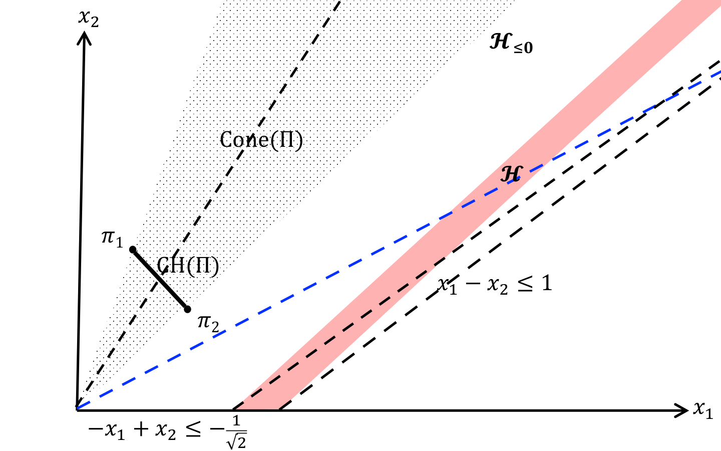
Figure 1 illustrates two examples with q=2q=2 and Π={π1,π2}\Pi=\{\pi_{1},\pi_{2}\}, where π1=(13,23)\pi_{1}=(\frac{1}{3},\frac{2}{3}) and π2=(12,12)\pi_{2}=(\frac{1}{2},\frac{1}{2}). In both examples, CH​(Π)\text{CH}(\Pi) is the line segment between π1\pi_{1} and π2\pi_{2}, Cone​(Π)\text{Cone}(\Pi) is the shaded area, ℋ{\mathcal{H}} is the red area, ℋ⩽0{\mathcal{H}}_{\leqslant 0} is the blue area, the intersection of ℋ{\mathcal{H}} and ℋ⩽0{\mathcal{H}}_{\leqslant 0} is the purple area, and ℋn{\mathcal{H}}_{n} is the green line segment. A key difference between Figure 1 (a) and (b) is whether CH​(Π)∩ℋ⩽0=∅\text{CH}(\Pi)\cap{\mathcal{H}}_{\leqslant 0}=\emptyset (which is true in Figure 1 (a) but not in (b)). Also it is possible that ℋ⩽0⊈ℋ{\mathcal{H}}_{\leqslant 0}\nsubseteq{\mathcal{H}}, as can be seen in Figure 1 (b).

Refer to caption Refer to caption
(a) 𝐀=[−341−2]{\mathbf{A}}=\left[\begin{array}[]{rr}-3&4\\ 1&-2\end{array}\right] and b→=[11]\vec{b}=\left[\begin{array}[]{r}1\\ 1\end{array}\right]. (b) 𝐀=[−111−20−1]{\mathbf{A}}=\left[\begin{array}[]{rr}-1&1\\ 1&-2\\ 0&-1\end{array}\right] and b→=[−1210.1]\vec{b}=\left[\begin{array}[]{r}-\frac{1}{\sqrt{2}}\\ 1\\ 0.1\end{array}\right].
Figure 1: Two examples of ℋ{\mathcal{H}}, ℋ⩽0{\mathcal{H}}_{\leqslant 0}, ℋn{\mathcal{H}}_{n}, CH​(Π)\text{CH}(\Pi), and Cone​(Π)\text{Cone}(\Pi).
A high-level attempt at the PMV-in-Polyhedron problem.

Before formally presenting the theorem, let us take a high-level attempt to develop intuition. Take the upper bound supπ→∈ΠnPr⁡(X→π→∈ℋ)\sup\nolimits_{\vec{\pi}\in\Pi^{n}}\Pr({\vec{X}}_{\vec{\pi}}\in{\mathcal{H}}) for example, there are three cases.

∙\bullet The 𝟎0 case. Clearly, if ℋ{\mathcal{H}} does not contain any non-negative integer whose L1L_{1} norm is nn, which is equivalent to ℋnℤ=∅{\mathcal{H}}_{n}^{\mathbb{Z}}=\emptyset, then supπ→∈ΠnPr⁡(X→π→∈ℋ)=0\sup\nolimits_{\vec{\pi}\in\Pi^{n}}\Pr({\vec{X}}_{\vec{\pi}}\in{\mathcal{H}})=0.

∙\bullet The exponential case (Figure 1 (a)). Suppose ℋnℤ≠∅{\mathcal{H}}_{n}^{\mathbb{Z}}\neq\emptyset. For any π→=(π1,…,πn)∈Πn\vec{\pi}=(\pi_{1},\ldots,\pi_{n})\in\Pi^{n} chosen by the max-adversary, we have π→⋅1→=∑j=1nπj∈Cone​(Π)\vec{\pi}\cdot\vec{1}=\sum_{j=1}^{n}\pi_{j}\in\text{Cone}(\Pi). According to various multivariate central limit theorems, X→π→{\vec{X}}_{\vec{\pi}} is “centered” around an Θ⁡(n)\Theta(\sqrt{n}) neighborhood of π→⋅1→\vec{\pi}\cdot\vec{1} with high probability. Therefore, if π→⋅1→\vec{\pi}\cdot\vec{1} is Θ⁡(n)\Theta(n) away from ℋ{\mathcal{H}}, then supπ→∈ΠnPr⁡(X→π→∈ℋ)\sup\nolimits_{\vec{\pi}\in\Pi^{n}}\Pr({\vec{X}}_{\vec{\pi}}\in{\mathcal{H}}) is exponentially small. This happens when CH​(Π)∩ℋ⩽0=∅\text{CH}(\Pi)\cap{\mathcal{H}}_{\leqslant 0}=\emptyset as shown in Figure 1 (a).

∙\bullet The polynomial case (Figure 1 (b)). Otherwise we have CH​(Π)∩ℋ⩽0≠∅\text{CH}(\Pi)\cap{\mathcal{H}}_{\leqslant 0}\neq\emptyset as shown in Figure 1 (b). In this case, the max-adversary can choose π→∈Πn\vec{\pi}\in\Pi^{n} such that π→⋅1→\vec{\pi}\cdot\vec{1} is either in Cone​(Π)\text{Cone}(\Pi) or close to it, which means that supπ→∈ΠnPr⁡(X→π→∈ℋ)\sup\nolimits_{\vec{\pi}\in\Pi^{n}}\Pr({\vec{X}}_{\vec{\pi}}\in{\mathcal{H}}) should be larger than that in the exponential case. However, it is not immediately clear that the probability is polynomial, because π→⋅1→\vec{\pi}\cdot\vec{1} being close to Cone​(Π)\text{Cone}(\Pi) and ℋnℤ≠∅{\mathcal{H}}_{n}^{\mathbb{Z}}\neq\emptyset does not immediately imply that X→π→{\vec{X}}_{\vec{\pi}} is close to ℋnℤ{\mathcal{H}}_{n}^{\mathbb{Z}}. Even if we assume that X→π→{\vec{X}}_{\vec{\pi}} is close to some (integer) vectors in ℋnℤ{\mathcal{H}}_{n}^{\mathbb{Z}}, it is unclear how “dense” such vectors are in the Θ⁡(n)\Theta(\sqrt{n}) neighborhood of π→⋅1→\vec{\pi}\cdot\vec{1}, which X→π→{\vec{X}}_{\vec{\pi}} falls into with high probability. In fact, accurately bounding the probability in the polynomial case is the most challenging part of the problem, because existing asymptotic tools fail to work due to their O⁡(n−0.5)O(n^{-0.5}) error terms.

The main technical theorem below confirms the intuition developed above when Π\Pi is closed and strictly positive (see Definition 5), and the answer to the polynomial case is Θ⁡(ndim(ℋ⩽0)−q2)\Theta\left(n^{\frac{\dim({\mathcal{H}}_{\leqslant 0})-q}{2}}\right), which is often much smaller than n−0.5n^{-0.5}.

Theorem 1 (Smoothed Likelihood of PMV-in-polyhedron).

Given any q∈ℕq\in\mathbb{N}, any closed and strictly positive Π\Pi over [q][q], and any polyhedron ℋ{\mathcal{H}} characterized by an integer matrix 𝐀{\mathbf{A}}, for any n∈ℕn\in\mathbb{N},

supπ→∈ΠnPr⁡(X→π→∈ℋ)={0if ​ℋnℤ=∅exp⁡(−Θ⁡(n))if ​ℋnℤ≠∅​ and ​ℋ⩽0∩CH​(Π)=∅Θ⁡(ndim(ℋ⩽0)−q2)otherwise (i.e. ​ℋnℤ≠∅​ and ​ℋ⩽0∩CH​(Π)≠∅​),\displaystyle\sup_{\vec{\pi}\in\Pi^{n}}\Pr\left({\vec{X}}_{\vec{\pi}}\in{\mathcal{H}}\right)=\left\{\begin{array}[]{ll}0&\text{if }{\mathcal{H}}_{n}^{\mathbb{Z}}=\emptyset\\ \exp(-\Theta(n))&\text{if }{\mathcal{H}}_{n}^{\mathbb{Z}}\neq\emptyset\text{ and }{\mathcal{H}}_{\leqslant 0}\cap\text{CH}(\Pi)=\emptyset\\ \Theta\left(n^{\frac{\dim({\mathcal{H}}_{\leqslant 0})-q}{2}}\right)&\text{otherwise (i.e. }{\mathcal{H}}_{n}^{\mathbb{Z}}\neq\emptyset\text{ and }{\mathcal{H}}_{\leqslant 0}\cap\text{CH}(\Pi)\neq\emptyset\text{)}\end{array}\right.,
infπ→∈ΠnPr⁡(X→π→∈ℋ)={0if ​ℋnℤ=∅exp⁡(−Θ⁡(n))if ​ℋnℤ≠∅​ and Θ⁡(ndim(ℋ⩽0)−q2)otherwise (i.e. ​ℋnℤ≠∅​ and CH​(Π)⊆ℋ⩽0​)\displaystyle\inf_{\vec{\pi}\in\Pi^{n}}\Pr\left({\vec{X}}_{\vec{\pi}}\in{\mathcal{H}}\right)=\left\{\begin{array}[]{ll}0&\text{if }{\mathcal{H}}_{n}^{\mathbb{Z}}=\emptyset\\ \exp(-\Theta(n))&\text{if }{\mathcal{H}}_{n}^{\mathbb{Z}}\neq\emptyset\text{ and }\\ \ \Theta\left(n^{\frac{\dim({\mathcal{H}}_{\leqslant 0})-q}{2}}\right)&\text{otherwise (i.e. }{\mathcal{H}}_{n}^{\mathbb{Z}}\neq\emptyset\text{ and }\text{CH}(\Pi)\subseteq{\mathcal{H}}_{\leqslant 0}\text{)}\end{array}\right.
Remarks on the power of Theorem 1.

We believe that the main power of Theorem 2 is that it provides a systematic way of reducing probabilistic analysis (asymptotically tight upper and lower bounds for the PMV-in-Polyhedron problem) to worst-case non-probabilistic analysis, which are often easy to verify. In particular, when CH​(Π)\text{CH}(\Pi) can be represented by the convex hull of a finite number of vectors, whether ℋ⩽0∩CH​(Π)=∅{\mathcal{H}}_{\leqslant 0}\cap\text{CH}(\Pi)=\emptyset and/or CH​(Π)⊈ℋ⩽0\text{CH}(\Pi)\not\subseteq{\mathcal{H}}_{\leqslant 0} can be verified by linear programming. Take the sup\sup part of Theorem 1 in the setting of Example 2 for instance. Suppose ℋnℤ≠∅{\mathcal{H}}_{n}^{\mathbb{Z}}\neq\emptyset.

  • •

    In Figure 1 (a), it is easy to see that ℋ⩽0∩CH​(Π)=∅{\mathcal{H}}_{\leqslant 0}\cap\text{CH}(\Pi)=\emptyset. Therefore,

    ∀π→∈Πn,Pr⁡(X→π→∈ℋ)≤exp⁡(−Θ⁡(n))\forall\vec{\pi}\in\Pi^{n},\Pr\left({\vec{X}}_{\vec{\pi}}\in{\mathcal{H}}\right)\leq\exp(-\Theta(n))
  • •

    In Figure 1 (b), we have ℋ⩽0∩CH​(Π)={π2}≠∅{\mathcal{H}}_{\leqslant 0}\cap\text{CH}(\Pi)=\{\pi_{2}\}\neq\emptyset, CH​(Π)⊈ℋ⩽0\text{CH}(\Pi)\not\subseteq{\mathcal{H}}_{\leqslant 0}, and dim(ℋ⩽0)=2\dim({\mathcal{H}}_{\leqslant 0})=2. Therefore, for any sufficiently large nn (for which it is not hard to prove that ℋnℤ≠∅{\mathcal{H}}_{n}^{\mathbb{Z}}\neq\emptyset), we have

    ∀π→∈Πn,exp⁡(−Θ⁡(n))≤Pr⁡(X→π→∈ℋ)≤Θ⁡(n−2−22)=Θ⁡(1)\forall\vec{\pi}\in\Pi^{n},\exp(-\Theta(n))\leq\Pr\left({\vec{X}}_{\vec{\pi}}\in{\mathcal{H}}\right)\leq\Theta(n^{-\frac{2-2}{2}})=\Theta(1)

    Notice that both bounds are asymptotically tight. For example, the lower bound can be achieved by π→={π1}n\vec{\pi}=\{\pi_{1}\}^{n} and the upper bound can be achieved by π→={π2}n\vec{\pi}=\{\pi_{2}\}^{n}.

As an example of the inf part of Theorem 1, suppose π1\pi_{1} is replaced by π1′=(23,13)\pi_{1}^{\prime}=(\frac{2}{3},\frac{1}{3}) in Figure 1 (b). Then, CH​(Π)⊆ℋ⩽0\text{CH}(\Pi)\subseteq{\mathcal{H}}_{\leqslant 0}, which means that ∀π→∈Πn,Pr⁡(X→π→∈ℋ)≥Θ⁡(1)\forall\vec{\pi}\in\Pi^{n},\Pr\left({\vec{X}}_{\vec{\pi}}\in{\mathcal{H}}\right)\geq\Theta(1) and the lower bound is asymptotically tight.

Remarks on the generality and limitations of Theorem 1.

We believe that Theorem 1 is quite general, because first, it provides a dichotomy (more precisely, trichotomy) for the PMV-in-Polyhedron problem. Second, the upper and lower bounds are asymptotically tight. And third, the theorem works for arbitrary ℋ{\mathcal{H}} characterized by an integer matrix 𝒜\mathcal{A} and arbitrary b→\vec{b}, and any closed and strictly positive Π\Pi. As a notable special case, when Π\Pi contains a single distribution π\pi, the sup and inf parts of the theorem coincide, and the theorem characterizes the PMV-in-Polyhedron problem for i.i.d. PMVs.

The main limitations are, first, the constants in the asymptotic bounds depend on qq, Π\Pi, and ℋ{\mathcal{H}}, which are assumed to be fixed; and second, Π\Pi must be strictly positive. Nevertheless, we believe that the two limitations are mild at least in the social choice context, because as can be seen in the next section as well as in [67], applications of Theorem 1 (or more precisely, its extension to unions of multiple polyhedra in Theorem 2 in Section 3.1) answer open questions in social choice under a more general and realistic model than IC. Moreover, as commented in [67], many classical models, such as Mallows model and random utility models, are strictly positive.

Remarks on the comparison with [67, Lemma 1].

We first recall an equivalent and simplified version of [67, Lemma 1] as Lemma∗\ast below for easy reference.

Lemma∗\ast ([67, Lemma 1]).

Let ℋ={x→∈ℝq:𝐄⋅(x→)⊤=(0→)⊤​ and ​𝐒⋅(x→)⊤<(0→)⊤}{\mathcal{H}}=\{\vec{x}\in{\mathbb{R}}^{q}:{\mathbf{E}}\cdot\left(\vec{x}\right)^{\top}=\left(\vec{0}\right)^{\top}\text{ and }{\mathbf{S}}\cdot\left(\vec{x}\right)^{\top}<\left(\vec{0}\right)^{\top}\}, where 𝐄\mathbf{E} and 𝐒\mathbf{S} are integer matrices and 𝐄⋅(1→)⊤=(0→)⊤{\mathbf{E}}\cdot\left(\vec{1}\right)^{\top}=\left(\vec{0}\right)^{\top} and 𝐒⋅(1→)⊤=(0→)⊤{\mathbf{S}}\cdot\left(\vec{1}\right)^{\top}=\left(\vec{0}\right)^{\top}. Then, supπ→∈ΠnPr⁡(X→π→∈ℋ)\sup_{\vec{\pi}\in\Pi^{n}}\Pr\left({\vec{X}}_{\vec{\pi}}\in{\mathcal{H}}\right) is 00, exp⁡(−Ω⁡(n))\exp(-\Omega(n)), or O(n−Rank(𝐄)/2)O(n^{-\text{Rank}(\mathbf{E})/2}), and the poly bound is asymptotically tight for infinitely many n∈ℕn\in\mathbb{N}.

We believe that our Theorem 1 is a non-trivial and significant improvement of Lemma ∗\ast in the following three aspects.

First, Theorem 1 works for any polyhedron ℋ={x→:𝐀⋅(x→)⊤≤(b→)⊤}{\mathcal{H}}=\left\{\vec{x}:{\mathbf{A}}\cdot\left(\vec{x}\right)^{\top}\leq\left(\vec{b}\right)^{\top}\right\} with arbitrary integer matrix 𝐀{\mathbf{A}}, while Lemma∗\ast requires 𝐀⋅(1→)⊤=(0→)⊤{\mathbf{A}}\cdot\left(\vec{1}\right)^{\top}=\left(\vec{0}\right)^{\top} and also essentially requires that elements in b→\vec{b} to be either 00 or −1-1, which correspond to the 𝐄\mathbf{E} part and the 𝐒\mathbf{S} part in Lemma∗\ast, respectively.

Second, Theorem 1 provides asymptotically tight bounds, while Lemma∗\ast only claims that the bounds are asymptotically tight for infinitely many nn’s.

Third, Theorem 1 characterizes smoothed likelihood for the min-adversary, while Lemma∗\ast only works for the max-adversary. While the proof of the min-adversary part of Theorem 1 is similar to its max-adversary part, it is due to the improved techniques and lemmas (Lemma 1 and 2 in the appendix). Without them we do not see an easy way to generalize Lemma∗\ast to the min-adversary.

The proof can be found in Appendix A.1, where a proof sketch is presented in Appendix A.1.1 and the full proof is presented in Appendix A.1.2.

3.1 An Extension of Theorem 1 to Unions of Polyhedra

In this subsection, we present an extension of Theorem 1 to the union of I∈ℕI\in\mathbb{N} polyhedra, denoted by 𝒞=⋃i≤Iℋi{\mathcal{C}}=\bigcup_{i\leq I}{\mathcal{H}}_{i}, where ℋi={x→∈ℝq:𝐀i⋅(x→)⊤≤(b→i)⊤}{\mathcal{H}}_{i}=\{\vec{x}\in{\mathbb{R}}^{q}:{\mathbf{A}}_{i}\cdot\left(\vec{x}\right)^{\top}\leq\left(\vec{b}_{i}\right)^{\top}\} and 𝐀i{\mathbf{A}}_{i} is an integer matrix of qq columns. We define the PMV-in-𝒞{\mathcal{C}} problem similarly as the PMV-in-Polyhedron problem (Definition 4), except that ℋ{\mathcal{H}} is replaced by 𝒞{\mathcal{C}}.

Definition 6 (The PMV-in-𝒞{\mathcal{C}} problem).

Given q,I∈ℕq,I\in\mathbb{N}, 𝒞=⋃i≤Iℋi{\mathcal{C}}=\bigcup_{i\leq I}{\mathcal{H}}_{i}, where ∀i≤I\forall i\leq I, ℋi⊆ℝq{\mathcal{H}}_{i}\subseteq\mathbb{R}^{q} is a polyhedron, and a set Π\Pi of distributions over [q][q], we are interested in

the upper bound ​supπ→∈ΠnPr⁡(X→π→∈𝒞)​, and the lower bound​infπ→∈ΠnPr⁡(X→π→∈𝒞)\text{\bf the upper bound }\sup\nolimits_{\vec{\pi}\in\Pi^{n}}\Pr({\vec{X}}_{\vec{\pi}}\in{\mathcal{C}})\text{, and {\bf the lower bound}}\inf\nolimits_{\vec{\pi}\in\Pi^{n}}\Pr({\vec{X}}_{\vec{\pi}}\in{\mathcal{C}})

The key observation is the following straightforward inequality for every PMV X→π→{\vec{X}}_{\vec{\pi}}:

maxi≤I⁡Pr⁡(X→π→∈ℋi)≤Pr⁡(X→π→∈𝒞)≤∑i≤IPr⁡(X→π→∈ℋi)\max\nolimits_{i\leq I}\Pr\left({\vec{X}}_{\vec{\pi}}\in{\mathcal{H}}_{i}\right)\leq\Pr\left({\vec{X}}_{\vec{\pi}}\in{\mathcal{C}}\right)\leq\sum\nolimits_{i\leq I}\Pr\left({\vec{X}}_{\vec{\pi}}\in{\mathcal{H}}_{i}\right) (6)

See Figure 2 for an illustration of I=3I=3. Notice that the right hand side of (6) is no more than I⋅maxi≤I⁡Pr⁡(X→π→∈ℋi)I\cdot\max_{i\leq I}\Pr({\vec{X}}_{\vec{\pi}}\in{\mathcal{H}}_{i}), which is Θ⁡(maxi≤I⁡Pr⁡(X→π→∈ℋi))\Theta(\max\nolimits_{i\leq I}\Pr({\vec{X}}_{\vec{\pi}}\in{\mathcal{H}}_{i})) because II is a constant.

Refer to caption
Figure 2: Illustration of inequality (6), where 𝒞=ℋ1∪ℋ2∪ℋ3{\mathcal{C}}={\mathcal{H}}_{1}\cup{\mathcal{H}}_{2}\cup{\mathcal{H}}_{3}.


The high-level idea behind the extension is based on a weighted complete bipartite activation graph defined as follows, which represents the relationship between CH​(Π)\text{CH}(\Pi) and polyhedra in 𝒞{\mathcal{C}} in light of Theorem 1. Let ℋi,⩽0{\mathcal{H}}_{i,\leqslant 0} denote the characteristic cone of ℋi{\mathcal{H}}_{i}.

Definition 7 (Activation graph 𝒢𝚷,𝒞,n\mathcal{G}_{\Pi,{\mathcal{C}},n}).

For any set of distributions Π\Pi over [q][q], any 𝒞=⋃i=1Iℋi{\mathcal{C}}=\bigcup_{i=1}^{I}{\mathcal{H}}_{i}, and any n∈ℕn\in\mathbb{N}, ℋi{\mathcal{H}}_{i} is said to be active (at nn) if ℋi,nℤ≠∅{\mathcal{H}}_{i,n}^{\mathbb{Z}}\neq\emptyset; otherwise ℋi{\mathcal{H}}_{i} is said to be inactive (at nn). Moreover, we define the activation graph 𝒢Π,𝒞,n\mathcal{G}_{\Pi,{\mathcal{C}},n} as follows.

∙\bullet Vertices. The vertices are CH​(Π)\text{CH}(\Pi) and {ℋi:1≤i≤I}\{{\mathcal{H}}_{i}:1\leq i\leq I\}.

∙\bullet Edges and weights. There is an edge between each π∈CH​(Π)\pi\in\text{CH}(\Pi) and each ℋi{\mathcal{H}}_{i}, whose weight is

wn​(π,ℋi)≜{−∞if ​ℋi​ is inactive at ​n−nlog⁡notherwise, if ​π∉ℋi,⩽0dim(ℋi,⩽0)otherwisew_{n}(\pi,{\mathcal{H}}_{i})\triangleq\left\{\begin{array}[]{ll}-\infty&\text{if }{\mathcal{H}}_{i}\text{ is inactive at }n\\ -\frac{n}{\log n}&\text{otherwise, if }\pi\notin{\mathcal{H}}_{i,\leqslant 0}\\ \dim({\mathcal{H}}_{i,\leqslant 0})&\text{otherwise}\end{array}\right.

For example, in Figure 3, ℋ1{\mathcal{H}}_{1} is inactive at nn and both ℋ2{\mathcal{H}}_{2} and ℋ3{\mathcal{H}}_{3} are active, π∈ℋ1,⩽0∩ℋ2,⩽0\pi\in{\mathcal{H}}_{1,\leqslant 0}\cap{\mathcal{H}}_{2,\leqslant 0} and π∉ℋ3,⩽0\pi\notin{\mathcal{H}}_{3,\leqslant 0}. Notice that the weight on (π,ℋ2)(\pi,{\mathcal{H}}_{2}) is dim(ℋ2,⩽0)\dim({\mathcal{H}}_{2,\leqslant 0}) instead of dim(ℋ2)\dim({\mathcal{H}}_{2}).

Refer to caption
Figure 3: Illustration of an activation graph 𝒢Π,𝒞,n\mathcal{G}_{\Pi,{\mathcal{C}},n}.

Intuitively, the 00, exponential, and polynomial cases of Theorem 1 (applied to Π={π}\Pi=\{\pi\}) corresponds to the −∞-\infty edge, the −nlog⁡n-\frac{n}{\log n} edge, and the dim(ℋi,⩽0)\dim({\mathcal{H}}_{i,\leqslant 0}) edge, respectively. That is, for any π→∈Πn\vec{\pi}\in\Pi^{n} with ∑j=1nπj=n⋅π\sum_{j=1}^{n}\pi_{j}=n\cdot\pi, Pr⁡(X→π→∈ℋi)\Pr({\vec{X}}_{\vec{\pi}}\in{\mathcal{H}}_{i}) is roughly nn raise to the power of the weight between π\pi and ℋi{\mathcal{H}}_{i} in the activation graph, i.e., nwn​(π,ℋi)n^{w_{n}(\pi,{\mathcal{H}}_{i})}. In particular, n−∞=0n^{-\infty}=0 and n−nlog⁡n−q=exp⁡(−Θ⁡(n))n^{-\frac{n}{\log n}-q}=\exp(-\Theta(n)). 22 2 This is the reason behind using −nlog⁡n-\frac{n}{\log n}. Theorem 2 still holds if −nlog⁡n-\frac{n}{\log n} is replace by any finite negative number.

Therefore, according to (6), Pr⁡(X→π→∈𝒞)\Pr({\vec{X}}_{\vec{\pi}}\in{\mathcal{C}}) is primarily determined by the largest wn​(π,ℋi){w_{n}(\pi,{\mathcal{H}}_{i})}, i.e., the maximum weight of all edges connected to π\pi in the activation graph. This is formally defined as follows.

Definition 8 (Active dimension).

Given 𝒞{\mathcal{C}}, nn, and π∈ℝq\pi\in\mathbb{R}^{q}, we define maximum active dimension of 𝒞{\mathcal{C}} at π\pi and nn (active dimension at π\pi for short, when 𝒞{\mathcal{C}} and nn are clear from the context), denoted by dim𝒞,nmax(π){\dim_{{\mathcal{C}},n}^{\max}}(\pi), as follows.

dim𝒞,nmax(π)≜maxi≤I⁡wn​(π,ℋi){\dim_{{\mathcal{C}},n}^{\max}}(\pi)\triangleq\max\nolimits_{i\leq I}w_{n}(\pi,{\mathcal{H}}_{i})

Consequently, a max- (respectively, min-) adversary aims to choose π→=(π1,…,πn)∈Πn\vec{\pi}=(\pi_{1},\ldots,\pi_{n})\in\Pi^{n} to maximize (respectively, minimize) dim𝒞,nmax(1n​∑j=1nπj){\dim_{{\mathcal{C}},n}^{\max}}(\frac{1}{n}\sum_{j=1}^{n}\pi_{j}), which are characterized by αn\alpha_{n} (respectively, βn\beta_{n}) defined as follows.

αn≜max⁡dim𝒞,nmaxπ∈CH​(Π)⁡(π)\displaystyle\alpha_{n}\triangleq\max\nolimits_{\pi\in\text{CH}(\Pi)}{\dim_{{\mathcal{C}},n}^{\max}}(\pi)
βn≜min⁡dim𝒞,nmaxπ∈CH​(Π)⁡(π)\displaystyle\beta_{n}\triangleq\min\nolimits_{\pi\in\text{CH}(\Pi)}{\dim_{{\mathcal{C}},n}^{\max}}(\pi)

We note that αn\alpha_{n} and βn\beta_{n} depend on Π\Pi and 𝒞{\mathcal{C}}, which are often clear from the context. Also, by definition, αn=−∞\alpha_{n}=-\infty is equivalent to β=−∞\beta=-\infty, which is equivalent to 𝒞nℤ=∅{\mathcal{C}}_{n}^{\mathbb{Z}}=\emptyset. We are now ready to use αn\alpha_{n} and βn\beta_{n} to present the extension of Theorem 1 to the PMV-in-𝒞{\mathcal{C}} problem.

Theorem 2 (Smoothed Likelihood of PMV-in-𝒞{\mathcal{C}}).

Given any q,I∈ℕq,I\in\mathbb{N}, any closed and strictly positive Π\Pi over [q][q], and any 𝒞=⋃i∈Iℋi{\mathcal{C}}=\bigcup_{i\in I}{\mathcal{H}}_{i} characterized by integer matrices, for any n∈ℕn\in\mathbb{N},

supπ→∈ΠnPr⁡(X→π→∈𝒞)={0if ​αn=−∞exp⁡(−Θ⁡(n))if −∞<αn<0Θ⁡(nαn−q2)otherwise (i.e. ​αn>0​),\displaystyle\sup_{\vec{\pi}\in\Pi^{n}}\Pr\left({\vec{X}}_{\vec{\pi}}\in{\mathcal{C}}\right)=\left\{\begin{array}[]{ll}0&\text{if }\alpha_{n}=-\infty\\ \exp(-\Theta(n))&\text{if }-\infty<\alpha_{n}<0\\ \Theta\left(n^{\frac{\alpha_{n}-q}{2}}\right)&\text{otherwise (i.e. }\alpha_{n}>0\text{)}\end{array}\right.,
infπ→∈ΠnPr⁡(X→π→∈𝒞)={0if ​βn=−∞exp⁡(−Θ⁡(n))if −∞<βn<0Θ⁡(nβn−q2)otherwise (i.e. ​βn>0​).\displaystyle\inf_{\vec{\pi}\in\Pi^{n}}\Pr\left({\vec{X}}_{\vec{\pi}}\in{\mathcal{C}}\right)=\left\{\begin{array}[]{ll}0&\text{if }\beta_{n}=-\infty\\ \exp(-\Theta(n))&\text{if }-\infty<\beta_{n}<0\\ \Theta\left(n^{\frac{\beta_{n}-q}{2}}\right)&\text{otherwise (i.e. }\beta_{n}>0\text{)}\end{array}\right..

Roughly speaking, the max- (respectively, min-) smoothed likelihood for an (n,q)(n,q)-PMV to be in 𝒞{\mathcal{C}} is approximately nαn−q2n^{\frac{\alpha_{n}-q}{2}} (respectively, nβn−q2n^{\frac{\beta_{n}-q}{2}}). The proof is done by combining the applications of Theorem 1 to Π\Pi and every ℋi{\mathcal{H}}_{i}, and can be found in Appendix A.2.

Remarks on the applications of Theorem 2.

We believe that Theorem 2 is a useful and general tool to study the smoothed likelihood of many events and properties in social choice, as shown in [67] as well as in the rest of this paper. Like Theorem 1, the power of Theorem 2 is that it provides a systematic way of reducing probabilistic analysis to worst-case and non-probabilistic analysis, i.e., the characterizations of αn\alpha_{n}, and βn\beta_{n}. Nevertheless, characterizing αn\alpha_{n} and βn\beta_{n} can still be challenging, which is equivalent to characterizing active ℋi{\mathcal{H}}_{i}, ℋi,⩽0{\mathcal{H}}_{i,\leqslant 0}, and dim(ℋi,⩽0)\dim({\mathcal{H}}_{i,\leqslant 0}), as we will see in the next section.

4 Smoothed Likelihood of Ties

In this section, we apply Theorem 2 to provide dichotomous characterizations of the smoothed likelihood of ties (Definition 2) under some commonly studied voting rules.

4.1 Integer Positional Scoring Rules

We first apply Theorem 2 to polyhedra that are similar to those in Example 1 and obtain the following theorem for integer positional scoring rules.

Theorem 3 (Smoothed likelihood of ties: integer positional scoring rules).

For any fixed m≥3m\geq 3, let ℳ=(Θ,ℒ⁡(𝒜),Π)\mathcal{M}=(\Theta,\mathcal{L}(\mathcal{A}),\Pi) be a strictly positive and closed single-agent preference model and let s→\vec{s} be an integer scoring vector. For any 2≤k≤m2\leq k\leq m and any n∈ℕn\in\mathbb{N},

Tie~Πmax​(rs→,k,n)\displaystyle\widetilde{\text{Tie}}^{\max}_{\Pi}(r_{\vec{s}},k,n) ={0if ​∀P∈ℒ​(𝒜)n,|rs→​(P)|≠kexp⁡(−Θ⁡(n))otherwise, if ​∀π∈CH​(Π),|rs→​(π)|<kΘ⁡(n−k−12)otherwise,\displaystyle=\left\{\begin{array}[]{ll}0&\text{if }\forall P\in\mathcal{L}(\mathcal{A})^{n},|r_{\vec{s}}(P)|\neq k\\ \exp(-\Theta(n))&\text{otherwise, if }\forall\pi\in\text{CH}(\Pi),|r_{\vec{s}}(\pi)|<k\\ \Theta(n^{-\frac{k-1}{2}})&\text{otherwise}\end{array}\right.,
Tie~Πmin​(rs→,k,n)\displaystyle\widetilde{\text{Tie}}^{\min}_{\Pi}(r_{\vec{s}},k,n) ={0if ​∀P∈ℒ​(𝒜)n,|rs→​(P)|≠kexp⁡(−Θ⁡(n))otherwise, if ​∃π∈CH​(Π)​ s.t. ​|rs→​(π)|<kΘ⁡(n−k−12)otherwise.\displaystyle=\left\{\begin{array}[]{ll}0&\text{if }\forall P\in\mathcal{L}(\mathcal{A})^{n},|r_{\vec{s}}(P)|\neq k\\ \exp(-\Theta(n))&\text{otherwise, if }\exists\pi\in\text{CH}(\Pi)\text{ s.t. }|r_{\vec{s}}(\pi)|<k\\ \Theta(n^{-\frac{k-1}{2}})&\text{otherwise}\end{array}\right..

Take the max smoothed likelihood of ties in Theorem 2 for example. Like Theorem 1, the condition for the 00 case is trivial. Assuming that the 00 case does not happen, the exponential case happens if no distribution (viewed as a fraction profile) in the convex hull of Π\Pi has at least kk winners under rs→r_{\vec{s}}. Otherwise, the polynomial case happens. That is, there exists an nn-profile PP with exactly kk winners under rs→r_{\vec{s}}, and there exists π∈CH​(Π)\pi\in\text{CH}(\Pi) that has at least kk winners. Notice that the existence of such PP (which depends on nn but not Π\Pi) does not imply the existence of such π\pi (which depends on Π\Pi but not nn), nor vice versa. All proofs in this section are delegated to Appendix C.

We immediately have the follow corollary of Theorem 3 when the uniform distribution πuni{\pi}_{\text{uni}} is in CH​(Π)\text{CH}(\Pi), because rs→​(πuni)=𝒜r_{\vec{s}}({\pi}_{\text{uni}})=\mathcal{A} and |𝒜|=m≥k|\mathcal{A}|=m\geq k, which means that the exponential case never happends. Notice that the corollary does not require πuni∈Π{\pi}_{\text{uni}}\in\Pi.

Corrollary 1 (Max smoothed likelihood of ties: positional scoring rules).

For any fixed m≥3m\geq 3, let ℳ=(Θ,ℒ⁡(𝒜),Π)\mathcal{M}=(\Theta,\mathcal{L}(\mathcal{A}),\Pi) be a strictly positive and closed single-agent preference model with πuni∈CH​(Π){\pi}_{\text{uni}}\in\text{CH}(\Pi). For any integer scoring vector s→\vec{s} and any k≤mk\leq m, for any n∈ℕn\in\mathbb{N},

Tie~Πmax​(rs→,k,n)={0if ​∀P∈ℒ​(𝒜)n,|rs→​(P)|≠kΘ⁡(n−k−12)otherwise.\hfill\widetilde{\text{Tie}}^{\max}_{\Pi}(r_{\vec{s}},k,n)=\left\{\begin{array}[]{ll}0&\text{if }\forall P\in\mathcal{L}(\mathcal{A})^{n},|r_{\vec{s}}(P)|\neq k\\ \Theta(n^{-\frac{k-1}{2}})&\text{otherwise}\end{array}\right..\hfill

The 00 case can indeed happen, for example, when rr is the plurality rule, k=mk=m, and m∤nm\nmid n. As commented in [67], πuni∈CH​(Π){\pi}_{\text{uni}}\in\text{CH}(\Pi) is a natural assumption that holds for many single-agent preference models. In particular, Corollary 1 works for IC, which corresponds to Π={πuni}\Pi=\{{\pi}_{\text{uni}}\}.

4.2 Edge-Order-Based Rules

The characterization for edge-order-based rules is more complicated due to the hardness in characterizing active ℋi{\mathcal{H}}_{i}, ℋi,⩽0{\mathcal{H}}_{i,\leqslant 0}, and dim(ℋi,⩽0)\dim({\mathcal{H}}_{i,\leqslant 0}) in the polyhedra representation of kk-way ties. We first introduce necessary notation to formally define edge-order-based rules, whose winners only depend on the order over all edges in WMG w.r.t. their weights, called palindromic orders.

Definition 9 (Palindromic orders).

A total preorder OO over ℰ={(a,b)∈𝒜×𝒜:a≠b}\mathcal{E}=\{(a,b)\in\mathcal{A}\times\mathcal{A}:a\neq b\} is palindromic, if for any pair of edges (a,b),(c,d)(a,b),(c,d) in ℰ\mathcal{E}, (a,b)⊳O(c,d)(a,b)\rhd_{O}(c,d) if and only if (d,c)⊳O(b,a)(d,c)\rhd_{O}(b,a), where e1⊳Oe2e_{1}\rhd_{O}e_{2} means that e1e_{1} is ranked strictly above e2e_{2} in OO, and e1≡Oe2e_{1}\equiv_{O}e_{2} means that e1e_{1} and e2e_{2} are tied in OO. Let 𝒪𝒜\mathcal{O}_{\mathcal{A}} denote the set of all palindromic orders over ℰ\mathcal{E}.

For any weighted directed graph GG over 𝒜\mathcal{A} with weights {w⁡(a,b):a≠b}\{w(a,b):a\neq b\} such that w⁡(a,b)=−w⁡(b,a)w(a,b)=-w(b,a), let EO​(G)∈𝒪𝒜\text{EO}(G)\in\mathcal{O}_{\mathcal{A}} denote the palindromic order w.r.t. the decreasing order of weights in GG. For any profile PP, let EO​(P)=EO​(WMG​(P))\text{EO}(P)=\text{EO}(\text{WMG}(P)).

In this paper we often use the tier representation of palindromic orders, which partition edges into equivalent classes (tiers).

Definition 10 (Tier representation and refinement of palindromic orders).

Any palindromic order O∈𝒪𝒜O\in\mathcal{O}_{\mathcal{A}} can be partitioned into tiers:

O=T1⊳⋯⊳Tt⊳T0⊳Tt+1⊳⋯⊳T2​t,O=T_{1}\rhd\cdots\rhd T_{t}\rhd T_{0}\rhd T_{t+1}\rhd\cdots\rhd T_{2t},

where for each 1≤i≤t1\leq i\leq t, edges in TiT_{i} are tied, edges in T2​t+1−iT_{2t+1-i} are tied, and edges in T2​t+1−iT_{2t+1-i} are obtained by flipping edges in TiT_{i}. T0T_{0} is called the middle tier, which consists of all edges ee with e≡Oe¯e\equiv_{O}\bar{e}, where e¯\bar{e} represents flipped ee. Only T0T_{0} is allowed to be empty. Let Ties​(O)=∑i=1t(|Ti|−1)+|T0|/2\text{Ties}(O)=\sum_{i=1}^{t}(|T_{i}|-1)+|T_{0}|/2.

O1∈𝒪𝒜O_{1}\in\mathcal{O}_{\mathcal{A}} refines O2∈𝒪𝒜O_{2}\in\mathcal{O}_{\mathcal{A}}, if for all pair of elements (e1,e2)(e_{1},e_{2}), e1⊳O2e2e_{1}\rhd_{O_{2}}e_{2} implies e1⊳O1e2e_{1}\rhd_{O_{1}}e_{2}.

Example 3.

Figure 4 illustrates an example of a profile PP, its WMG, and its corresponding palindromic order. In Figure 4 (b) only edges with positive weights are shown.

{1≻2≻3,1≻3≻2}\{1\succ 2\succ 3,1\succ 3\succ 2\} {(1,2),(1,3)}⏟T1⊳{(2,3),(3,2)}⏟T0⊳{(2,1),(3,1)}⏟T2\underbrace{\{(1,2),(1,3)\}}_{T_{1}}\rhd\underbrace{\{(2,3),(3,2)\}}_{T_{0}}\rhd\underbrace{\{(2,1),(3,1)\}}_{T_{2}}
(a) Profile PP. (b) WMG​(P)\text{WMG}(P). (c) EO​(P)\text{EO}(P).
Figure 4: An example of a profile, its WMG, and its palindromic order.

Let O={(1,2)}⏟T1⊳{(1,3)}⏟T2⊳{(2,3),(3,2)}⏟T0⊳{(3,1)}⏟T3⊳{(2,1)}⏟T4O=\underbrace{\{(1,2)\}}_{T_{1}}\rhd\underbrace{\{(1,3)\}}_{T_{2}}\rhd\underbrace{\{(2,3),(3,2)\}}_{T_{0}}\rhd\underbrace{\{(3,1)\}}_{T_{3}}\rhd\underbrace{\{(2,1)\}}_{T_{4}}. We have Ties​(EO​(P))=3\text{Ties}(\text{EO}(P))=3, Ties​(O)=1\text{Ties}(O)=1, and OO refines EO​(P)\text{EO}(P).

We are now ready to formally define edge-order-based rules using palindromic orders.

Definition 11 (Edge-order-based rules).

A voting rule rr is said to be edge-order-based, if for every pair of profiles P1,P2P_{1},P_{2} with EO​(P1)=EO​(P2)\text{EO}(P_{1})=\text{EO}(P_{2}), we have r⁡(P1)=r⁡(P2)r(P_{1})=r(P_{2}).

Many WMG-based rules, such as Copeland, Maximin, Schulze, and ranked pairs, are edge-order-based. The domain of any edge-order-based rule rr can be naturally extended to palindromic orders. When applying Theorem 2 to edge-order-based rules, each polyhedron ℋi{\mathcal{H}}_{i} in 𝒞{\mathcal{C}} is indexed by a palindromic order OO with kk co-winners, such that ℋi,nℤ{\mathcal{H}}_{i,n}^{\mathbb{Z}} corresponds to the histograms of nn-profiles whose edge orders are OO.

We now define and characterize palindromic orders obtained from nn-profiles.

Definition 12.

For any n∈ℕn\in\mathbb{N}, let 𝒪𝒜n≜{EO​(P):P∈ℒ​(𝒜)n}\mathcal{O}_{\mathcal{A}}^{n}\triangleq\{\text{EO}(P):P\in\mathcal{L}(\mathcal{A})^{n}\}. Let 𝒪𝒜′⊂𝒪𝒜\mathcal{O}_{\mathcal{A}}^{\prime}\subset\mathcal{O}_{\mathcal{A}} denote the set of palindromic orders OO whose middle tier is empty.

Proposition 1.

For any 𝒜\mathcal{A} and any n≥m4n\geq m^{4}, 𝒪𝒜n={𝒪𝒜if ​2|n𝒪𝒜′if ​2∤n\mathcal{O}_{\mathcal{A}}^{n}=\left\{\begin{array}[]{ll}\mathcal{O}_{\mathcal{A}}&\text{if }2\mid n\\ \mathcal{O}_{\mathcal{A}}^{\prime}&\text{if }2\nmid n\\ \end{array}\right..

The proof of Proposition 1 is delegated to Appendix C.1. Next, we define 𝒪r,k,nπ\mathcal{O}_{r,k,n}^{\pi} as the set of palindromic orders OO that satisfies three conditions: (1) O∈𝒪𝒜nO\in\mathcal{O}_{\mathcal{A}}^{n}; (2) there are exactly kk winners in OO under rr, and (3) OO refines EO​(π)\text{EO}(\pi), where π\pi is viewed as a fractional profile. Let 𝒪r,k,nΠ≜⋃π∈CH​(Π)𝒪r,k,nπ\mathcal{O}_{r,k,n}^{\Pi}\triangleq\bigcup_{\pi\in\text{CH}(\Pi)}\mathcal{O}_{r,k,n}^{\pi}. When 𝒪r,k,nΠ≠∅\mathcal{O}_{r,k,n}^{\Pi}\neq\emptyset, we let ℓmin\ell_{\min} denote the minimum number of ties in palindromic orders in 𝒪r,k,nΠ\mathcal{O}_{r,k,n}^{\Pi}. When 𝒪r,k,nΠ≠∅\mathcal{O}_{r,k,n}^{\Pi}\neq\emptyset, we let ℓmm\ell_{\text{mm}} denote the maximin number of ties, where the maximum is taken for all π∈CH​(Π)\pi\in\text{CH}(\Pi), and for any given π\pi, the minimum is taken for all palindromic orders in 𝒪r,k,nπ\mathcal{O}_{r,k,n}^{\pi}. We note that ℓmin\ell_{\min} and ℓmm\ell_{\text{mm}} depend on Π\Pi, rr, kk, and nn, which are clear from the context. The formal definitions can be found in Appendix C.2. In fact, ℓmin\ell_{\min} and ℓmm\ell_{\text{mm}} correspond to m!−αnm!-\alpha_{n} and m!−βnm!-\beta_{n} in Theorem 2. We are now ready to present the theorem for EO-based rules.

Theorem 4 (Smoothed likelihood of ties: edge-order-based rules).

For any fixed m≥3m\geq 3, let ℳ=(Θ,ℒ⁡(𝒜),Π)\mathcal{M}=(\Theta,\mathcal{L}(\mathcal{A}),\Pi) be a strictly positive and closed single-agent preference model and let rr be an edge-order-based rule. For any 2≤k≤m2\leq k\leq m and any n∈ℕn\in\mathbb{N},

Tie~Πmax​(r,k,n)={0if ​∀O∈𝒪𝒜n,|r⁡(O)|≠kexp⁡(−Θ⁡(n))otherwise if ​𝒪r,k,nΠ=∅Θ⁡(n−ℓmin2)otherwise\displaystyle\widetilde{\text{Tie}}^{\max}_{\Pi}(r,k,n)=\left\{\begin{array}[]{ll}0&\text{if }\forall O\in\mathcal{O}_{\mathcal{A}}^{n},|r(O)|\neq k\\ \exp(-\Theta(n))&\text{otherwise if }\mathcal{O}_{r,k,n}^{\Pi}=\emptyset\\ \Theta\left(n^{-\frac{\ell_{\min}}{2}}\right)&\text{otherwise}\end{array}\right.
Tie~Πmin​(r,k,n)={0if ​∀O∈𝒪𝒜n,|r⁡(O)|≠kexp⁡(−Θ⁡(n))otherwise if ​∃π∈CH​(Π)​ s.t. ​𝒪r,k,nπ=∅Θ⁡(n−ℓmm2)otherwise\displaystyle\widetilde{\text{Tie}}^{\min}_{\Pi}(r,k,n)=\left\{\begin{array}[]{ll}0&\text{if }\forall O\in\mathcal{O}_{\mathcal{A}}^{n},|r(O)|\neq k\\ \exp(-\Theta(n))&\text{otherwise if }\exists\pi\in\text{CH}(\Pi)\text{ s.t. }\mathcal{O}_{r,k,n}^{\pi}=\emptyset\\ \Theta\left(n^{-\frac{\ell_{\text{mm}}}{2}}\right)&\text{otherwise}\end{array}\right.

The proof can be found in Appendix C.3. In the remainder of this section, we apply Theorem 4 to provide dichotomous characterizations of max\max-smooth likelihood of ties under Copelandα, maximin, Schulze, and ranked pairs for the model in Corollary 1, which includes IC as a special case.

Proposition 2 (Max smoothed likelihood of ties: Copelandα).

For any fixed m≥3m\geq 3, let ℳ=(Θ,ℒ⁡(𝒜),Π)\mathcal{M}=(\Theta,\mathcal{L}(\mathcal{A}),\Pi) be a strictly positive and closed single-agent preference model with πuni∈CH​(Π){\pi}_{\text{uni}}\in\text{CH}(\Pi). Let lα=min⁡{t∈ℕ:t​α∈ℤ}l_{\alpha}=\min\{t\in{\mathbb{N}}:t\alpha\in\mathbb{Z}\}. For any 2≤k≤m2\leq k\leq m and any n∈ℕn\in\mathbb{N},

Tie~Πmax​(Cdα,k,n)={0if ​2∤n,2|k,and ​k≥m−1Θ⁡(n−k4)if ​2|n,2|k,a​n​d​{(1)​k=m, or(2)​k=m−1​ and ​α≥12, or(3)​k=m−1​ and ​k≤lα​(lα+1)Θ⁡(n−lα​(lα+1)4)if ​2|n,2|k,k=m−1,α⁡<12, and ​k>​lα​(lα+1)Θ⁡(1)otherwise (i.e., if ​2∤k​ or ​k≤m−2​)\widetilde{\text{Tie}}^{\max}_{\Pi}(\text{Cd}_{\alpha},k,n)=\left\{\begin{array}[]{ll}0&\text{if }2\nmid n,2\mid k,\text{and }k\geq m-1\\ \Theta(n^{-\frac{k}{4}})&\text{if }2\mid n,2\mid k,{and}\left\{\begin{array}[]{l}(1)k=m,\text{ or}\\ (2)k=m-1\text{ and }\alpha\geq\frac{1}{2},\text{ or}\\ (3)k=m-1\text{ and }k\leq l_{\alpha}(l_{\alpha}+1)\end{array}\right.\\ \Theta\left(n^{-\frac{l_{\alpha}(l_{\alpha}+1)}{4}}\right)&\text{if }2\mid n,2\mid k,k=m-1,\alpha<\frac{1}{2},\text{ and }k>l_{\alpha}(l_{\alpha}+1)\\ \Theta(1)&\text{otherwise (i.e., if }2\nmid k\text{ or }k\leq m-2\text{)}\end{array}\right.

The Θ⁡(1)\Theta(1) case appears most typical, which happens when kk is odd or k≤m−2k\leq m-2. The Θ⁡(n−lα​(lα+1)4)\Theta(n^{-\frac{l_{\alpha}(l_{\alpha}+1)}{4}}\ ) case appears most interesting, because its degree depends on the smallest natural number lαl_{\alpha} such that α​lα\alpha l_{\alpha} is an integer. For example, l0=1l_{0}=1, l1/3=3l_{1/3}=3, l2/5=5l_{2/5}=5, and lα=∞l_{\alpha}=\infty for any irrational number α\alpha (which means that the Θ⁡(n−lα​(lα+1)4)\Theta(n^{-\frac{l_{\alpha}(l_{\alpha}+1)}{4}}) case does not happen because k<∞=lα​(lα+1)k<\infty=l_{\alpha}(l_{\alpha}+1)). While the Θ⁡(1)\Theta(1) case can probably be proved by standard central limit theorem and the union bound, we are not aware of a previous work on it. Standard techniques are too coarse for other cases.

Proposition 3 (Max smoothed likelihood of ties: maximin).

For any fixed m≥3m\geq 3, let ℳ=(Θ,ℒ⁡(𝒜),Π)\mathcal{M}=(\Theta,\mathcal{L}(\mathcal{A}),\Pi) be a strictly positive and closed single-agent preference model with πuni∈CH​(Π){\pi}_{\text{uni}}\in\text{CH}(\Pi). For any 2≤k≤m2\leq k\leq m and any n∈ℕn\in\mathbb{N}, Tie~Πmax​(MM,k,n)=Θ⁡(n−k−12)\widetilde{\text{Tie}}^{\max}_{\Pi}(\text{MM},k,n)=\Theta(n^{-\frac{k-1}{2}}).

Proposition 4 (Max smoothed likelihood of ties: Schulze).

For any fixed m≥3m\geq 3, let ℳ=(Θ,ℒ⁡(𝒜),Π)\mathcal{M}=(\Theta,\mathcal{L}(\mathcal{A}),\Pi) be a strictly positive and closed single-agent preference model with πuni∈CH​(Π){\pi}_{\text{uni}}\in\text{CH}(\Pi). For any 2≤k≤m2\leq k\leq m and any n∈ℕn\in\mathbb{N}, Tie~Πmax​(Sch,k,n)=Θ⁡(n−k−12)\widetilde{\text{Tie}}^{\max}_{\Pi}(\text{Sch},k,n)=\Theta(n^{-\frac{k-1}{2}}).

Proposition 5 (Max smoothed likelihood of ties: ranked pairs).

For any fixed m≥3m\geq 3, let ℳ=(Θ,ℒ⁡(𝒜),Π)\mathcal{M}=(\Theta,\mathcal{L}(\mathcal{A}),\Pi) be a strictly positive and closed single-agent preference model with πuni∈CH​(Π){\pi}_{\text{uni}}\in\text{CH}(\Pi). For any 2≤k≤m2\leq k\leq m and any n∈ℕn\in\mathbb{N}, Ω⁡(n−k−12)≤Tie~Πmax​(RP,k,n)≤n−Ω⁡(log⁡klog⁡log⁡k)\Omega(n^{-\frac{k-1}{2}})\leq\widetilde{\text{Tie}}^{\max}_{\Pi}(\text{RP},k,n)\leq n^{-\Omega(\frac{\log k}{\log\log k})}. Moreover, when m≥k+5​⌈log⁡k⌉m\geq k+5\lceil\log k\rceil, Tie~Πmax​(RP,k,n)=Ω⁡(n−⌈log⁡k⌉2)\widetilde{\text{Tie}}^{\max}_{\Pi}(\text{RP},k,n)=\Omega(n^{-\frac{\lceil\log k\rceil}{2}}). When k=2k=2, we have Tie~Πmax​(RP,2,n)=Θ⁡(n−0.5)\widetilde{\text{Tie}}^{\max}_{\Pi}(\text{RP},2,n)=\Theta(n^{-0.5}).

Proof sketches of Propositions 2, 3, 4, and 5. The proofs are done by applying Theorem 4. For any EO-based rules rr studied in this paper, the condition for the 00 case can be verified efficiently using Proposition 1 for any sufficiently large nn. If the 00 case does not happen, then the exponential case does not happen either, because for any O∈𝒪𝒜nO\in\mathcal{O}_{\mathcal{A}}^{n} such that |r⁡(O)|=k|r(O)|=k, OO extends EO​(πuni)\text{EO}({\pi}_{\text{uni}}), which is the palindromic order that only has the middle tier T0T_{0}. This also means that for every π∈CH​(Π)\pi\in\text{CH}(\Pi), we have 𝒪r,k,nπ⊆𝒪r,k,nπuni\mathcal{O}_{r,k,n}^{\pi}\subseteq\mathcal{O}_{r,k,n}^{{\pi}_{\text{uni}}}. Consequently, ℓmin\ell_{\text{min}} is achieved at πuni{\pi}_{\text{uni}}.

The bulk of proof then focuses on characterizing O∈𝒪𝒜nO\in\mathcal{O}_{\mathcal{A}}^{n} with the minimum number of ties such that |r⁡(O)|=k|r(O)|=k. This can be more complicated than it appears, for example for ranked pairs and for Copelandα when 2∤2\nmid and α\alpha is not 00 or 11. In particular, for ranked pairs we were only able to obtain (non-tight) upper and lower bounds. The full proofs of Propositions 2, 3, 4, and 5 can be found in Appendix C.4, C.5, C.6, and C.7, respectively. □\Box

4.3 STV and Coombs

Theorem 5 (Smoothed likelihood of ties: STV and Coombs).

For any fixed m≥3m\geq 3, let r∈{STV,Coombs}r\in\{\text{STV},\text{Coombs}\} and let ℳ=(Θ,ℒ⁡(𝒜),Π)\mathcal{M}=(\Theta,\mathcal{L}(\mathcal{A}),\Pi) be a strictly positive and closed single-agent preference model. For any 2≤k≤m2\leq k\leq m and n∈ℕn\in\mathbb{N}, Tie~Πmax​(r,k,n)\widetilde{\text{Tie}}^{\max}_{\Pi}(r,k,n) (respectively, Tie~Πmin​(rs→,k,n)\widetilde{\text{Tie}}^{\min}_{\Pi}(r_{\vec{s}},k,n)) is either 00, exp⁡(−Θ⁡(n))\exp(-\Theta(n)), or Θ​(poly​(n))\Theta(\text{poly}(n)).

The formal statement of the theorem and its proof are delegated to Appendix D. To accurately characterize the degree in the polynomial case, we introduce PUT structures (Definition 21) as the counterpart of palindromic orders to define and analyze active polyhedra and the dimensions of their characteristic cones. See Appendix D for its formal definitions and an example. Like in Section 4.2, the theorem can be applied to characterize max smoothed likelihood of ties for STV and Coombs for distributions Π\Pi where πuni∈CH​(Π){\pi}_{\text{uni}}\in\text{CH}(\Pi), as shown in the following proposition.

Proposition 6 (Max smoothed likelihood of ties: STV and Coombs).

For any fixed m≥3m\geq 3, let r∈{STV,Coombs}r\in\{\text{STV},\text{Coombs}\} and let ℳ=(Θ,ℒ⁡(𝒜),Π)\mathcal{M}=(\Theta,\mathcal{L}(\mathcal{A}),\Pi) be a strictly positive and closed single-agent preference model with πuni∈CH​(Π){\pi}_{\text{uni}}\in\text{CH}(\Pi). For any 2≤k≤m2\leq k\leq m and any n∈ℕn\in\mathbb{N},

Tie~Πmax​(r,k,n)={Θ⁡(n−k−12)if ​{(1)​m≥4​, or (2)​m=3​ and ​k=2, or (3)​m=k=3​ and ​(2​∣n​ or ​3∣​n)0otherwise (i.e., ​m=k=3​, ​2∤n, and ​3∤n​)\widetilde{\text{Tie}}^{\max}_{\Pi}(r,k,n)=\left\{\begin{array}[]{ll}\Theta(n^{-\frac{k-1}{2}})&\text{if }\left\{\begin{array}[]{l}(1)m\geq 4\text{, or }\\ (2)m=3\text{ and }k=2,\text{ or }\\ (3)m=k=3\text{ and }(2\mid n\text{ or }3\mid n)\end{array}\right.\\ 0&\text{otherwise (i.e., }m=k=3\text{, }2\nmid n,\text{ and }3\nmid n\text{)}\end{array}\right.

To prove the proposition, we prove a McGarvey 1953-type result for STV and Coombs (Lemma 3) to characterize active polyhedra. The lemma might be of independent interest.

5 Experimental Studies

We examine the fraction of profiles with two-or-more-way ties using simulated data and Preflib data [42] under Borda, plurality, veto, maximin, ranked pairs, Schulze, Copeland0.5, STV, and Coombs. All experiments were implemented in Python 3 and were conducted on a MacOS laptop with 3.1 GHz Intel Core i7 CPU and 16 GB memory.
Simulated data. We generate profiles of m=4m=4 alternatives under IC. nn ranges from 2020 to 200200. In each setting we generate 100000100000 profiles. The goal of experiments on synthetic data is to provide a sanity check for the theoretical results in this paper. For clarity, we present the results for Borda, STV, maximin, ranked pairs, and Copeland0.5 in Figure 5. Results for all voting rules described above can be found in Figure 15 in Appendix E. Figure 5 confirms Corollary 1 and Propositions 2, 3, 5, and 6 under IC as discussed in the Introduction: the probability of any-way ties is Θ⁡(1)\Theta(1) for Copeland0.5 and is Θ⁡(1n)\Theta(\frac{1}{\sqrt{n}}) for other rules. [Uncaptioned image] Figure 5: Fraction of tied profiles under IC.

Preflib data.

Because the PUT versions of STV and ranked pairs are NP-hard to compute [14, 8], we used AI-search-based implementations of STV and ranked pairs [63] and computed the fraction of tied profiles among the 307 profiles from Strict Order-Complete Lists (SOC) under election data category at Preflib [42].33 3 Preflib mentioned that this category can be interpreted as election data, though not all of them come from real-life elections. See some statistics in Appendix E. We used the same dataset in [63], where PUT ranked pairs can finish in one hour. The results are summarized in Table 2 below. We emphasize that the observations are drawn only from Preflib data and should not be interpreted as general conclusions on the likelihood of ties in presidential elections.

Table 2: Percentage of tied profiles in Preflib data in weakly increasing order.
Borda Copeland0.5 Plurality Maximin Schulze Ranked pairs STV Coombs Veto
Ties 1.6% 2.6% 4.6% 6.8% 6.8% 6.8% 7.5% 10.4% 31.3%

Table 2 shows that ties occur least frequently under Borda (1.6% of the profiles), which is consistent with the experiments on synthetic data in Figure 5. Two interesting observations are: first, ties are rare under Copeland0.5 (2.6%); and second, ties occur frequently under veto (31.3%), which mostly happen when the number of alternatives is larger than the number of voters—in such cases the election is guaranteed to be tied under veto. The two observations are quite different from Figure 5, which is probably because real-life preference data can be significantly different from IC, as widely acknowledged in the literature [35].

6 Future work

We see three immediate directions for future work. First, technically, how can we improve the results for more general models, especially by dropping the strictness assumption on Π\Pi? Second, how can we extend the study to other events of interest in voting, for example, stability and margin of victory of voting rules, and more generally other topics such as multi-winner elections, judgement aggregation, matching, and resource allocation? Third, what are the smoothed complexity in various computational aspects of voting [5], such as winner determination [69], manipulation, bribery and control?

7 Acknowledgements

We thank Rupert Freeman, Qishen Han, Ao Liu, Marcus Pivato, Sikai Ruan, Rohit Vaish, Weiqiang Zheng, Bill Zwicker, participants of the COMSOC video seminar, and anonymous reviewers for helpful comments. This work is supported by NSF #1453542, ONR #N00014-17-1-2621, and a gift fund from Google.

References

  • [1]
  • Austen-Smith and Banks [1996] David Austen-Smith and Jeffrey S. Banks. 1996. Information Aggregation, Rationality, and the Condorcet Jury Theorem. The American Political Science Review 90, 1 (1996), 34–45.
  • Aziz et al. [2013] Haris Aziz, Serge Gaspers, Nicholas Mattei, Nina Narodytska, and Toby Walsh. 2013. Ties Matter: Complexity of Manipulation when Tie-Breaking with a Random Vote. In Proceedings of IJCAI.
  • Banzhaf III [1968] John F. Banzhaf III. 1968. One Man, 3.312 Votes: A Mathematical Analysis of the Electoral College. Villanova Law Review 13, 2 (1968), Article 3.
  • Baumeister et al. [2020] Dorothea Baumeister, Tobias Hogrebe, and Jörg Rothe. 2020. Towards Reality: Smoothed Analysis in Computational Social Choice. In Proceedings of AAMAS. 1691–1695.
  • Beck [1975] Nathaniel Beck. 1975. A note on the probability of a tied election. Public Choice 23, 1 (1975), 75–79.
  • Bentkus [2005] Vidmantas Bentkus. 2005. A Lyapunov-type bound in RdR^{d}. Theory of Probability & Its Applications 49, 2 (2005), 311—323.
  • Brill and Fischer [2012] Markus Brill and Felix Fischer. 2012. The Price of Neutrality for the Ranked Pairs Method. In Proceedings of the National Conference on Artificial Intelligence (AAAI). Toronto, Canada, 1299–1305.
  • Buchanan [1974] James M. Buchanan. 1974. Hegel on the Calculus of Voting. Public Choice 11 (1974), 99–101.
  • Campbell and Witcher [2015] Noel Campbell and Marcus Witcher. 2015. Political entrepreneurship: Jefferson, Bayard, and the election of 1800. Journal of Entrepreneurship and Public Policy 4, 3 (2015), 298–312.
  • Chamberlain and Rothschild [1981] Gary Chamberlain and Michael Rothschild. 1981. A note on the probability of casting a decisive vote. Journal of Economic Theory 25, 1 (1981), 152–162.
  • Chung et al. [2008] Christine Chung, Katrina Ligett, Kirk Pruhs, and Aaron Roth. 2008. The Price of Stochastic Anarchy. In International Symposium on Algorithmic Game Theory. 303–314.
  • Condorcet [1785] Marquis de Condorcet. 1785. Essai sur l’application de l’analyse à la probabilité des décisions rendues à la pluralité des voix. Paris: L’Imprimerie Royale.
  • Conitzer et al. [2009] Vincent Conitzer, Matthew Rognlie, and Lirong Xia. 2009. Preference Functions That Score Rankings and Maximum Likelihood Estimation. In Proceedings of the Twenty-First International Joint Conference on Artificial Intelligence (IJCAI). Pasadena, CA, USA, 109–115.
  • Conitzer and Walsh [2016] Vincent Conitzer and Toby Walsh. 2016. Barriers to Manipulation in Voting. In Handbook of Computational Social Choice, Felix Brandt, Vincent Conitzer, Ulle Endriss, Jérôme Lang, and Ariel Procaccia (Eds.). Cambridge University Press, Chapter 6.
  • Cook et al. [1986] William J. Cook, Albertus M. H. Gerards, Alexander Schrijver, and Eva Tardos. 1986. Sensitivity theorems in integer linear programming. Mathematical Programming 34, 3 (1986), 251–264.
  • Daskalakis et al. [2016] Constantinos Daskalakis, Anindya De, Gautam Kamat, and Christos Tzamos. 2016. A Size-Free CLT for Poisson Multinomials and its Applications. In Proceedings of STOC. 1074–1086.
  • Diakonikolas et al. [2016] Ilias Diakonikolas, Daniel Mertz Kane, and Alistair Stewart. 2016. The fourier transform of poisson multinomial distributions and its algorithmic applications. In Proceedings of STOC. 1060–1073.
  • Domb [1960] Cyril Domb. 1960. On the theory of cooperative phenomena in crystals. Advances in Physics 9, 34 (1960), 149–244.
  • Downs [1957] Anthony Downs. 1957. An Economic Theory of Democracy. New York: Harper & Row.
  • Faliszewski and Rothe [2016] Piotr Faliszewski and Jörg Rothe. 2016. Control and bribery in voting. In Handbook of Computational Social Choice. Cambridge University Press, Chapter 7.
  • Feddersen and Pesendorfer [1996] Timothy Feddersen and Wolfang Pesendorfer. 1996. The swing voter’s curse. American Economic Review 86 (1996), 408–424.
  • Freeman et al. [2015] Rupert Freeman, Markus Brill, and Vincent Conitzer. 2015. General Tiebreaking Schemes for Computational Social Choice. In Proceedings of the 2015 International Conference on Autonomous Agents and Multiagent Systems. 1401–1409.
  • Friedgut et al. [2011] Ehud Friedgut, Gil Kalai, Nathan Keller, and Noam Nisan. 2011. A Quantitative Version of the Gibbard-Satterthwaite theorem for Three Alternatives. SIAM J. Comput. 40, 3 (2011), 934–952.
  • Gelman et al. [1998] Andrew Gelman, Gary King, and John Boscardin. 1998. Estimating the Probability of Events that Have Never Occurred: When Is Your Vote Decisive? J. Amer. Statist. Assoc. 93 (1998), 1–9.
  • Gelman et al. [2012] Andrew Gelman, Nate Silver, and Aaron Edlin. 2012. What is the probability your vote will make a difference? Economic Inquiry 50, 2 (2012), 321–326.
  • Gibbard [1973] Allan Gibbard. 1973. Manipulation of voting schemes: A general result. Econometrica 41 (1973), 587–601.
  • Gillett [1977] Raphael Gillett. 1977. Collective Indecision. Behavioral Science 22, 6 (1977), 383–390.
  • Gillett [1980] Raphael Gillett. 1980. The Comparative Likelihood of an Equivocal Outcome under the Plurality, Condorcet, and Borda Voting Procedures. Public Choice 35, 4 (1980), 483–491.
  • Good and Mayer [1975] I. J. Good and Lawrence S. Mayer. 1975. Estimating the efficacy of a vote. Behavioral Science 20, 1 (1975), 25–33.
  • Hoeffding [1956] Wassily Hoeffding. 1956. On the Distribution of the Number of Successes in Independent Trials. The Annals of Mathematical Statistics 27, 3 (1956), 713–721.
  • Hoeffding [1963] Wassily Hoeffding. 1963. Probability inequalities for sums of bounded random variables. J. Amer. Statist. Assoc. 58, 301 (1963), 13—30.
  • Huang and Teng [2007] Li-Sha Huang and Shang-Hua Teng. 2007. On the Approximation and Smoothed Complexity of Leontief Market Equilibria. In Proceedings of FAW. 96–107.
  • Le Breton et al. [2016] Michel Le Breton, Dominique Lepelley, and Hatem Smaoui. 2016. Correlation, partitioning and the probability of casting a decisive vote under the majority rule. Journal of Mathematical Economics 64 (2016), 11–22.
  • Lehtinen and Kuorikoski [2007] Aki Lehtinen and Jaakko Kuorikoski. 2007. Unrealistic Assumptions in Rational Choice Theory. Philosophy of the Social Sciences 37, 2 (2007), 115–138.
  • Liu et al. [2020] Ao Liu, Yun Lu, Lirong Xia, and Vassilis Zikas. 2020. How Private Is Your Voting?. Presented at WADE-18 workshop. In Proceedings of UAI.
  • Lovász and Plummer [2009] L. Lovász and M.D. Plummer. 2009. Matching Theory. North-Holland; Elsevier Science Publishers B.V.; Sole distributors for the U.S.A. and Canada, Elsevier Science Publishing Company.
  • Magrino et al. [2011] Thomas R. Magrino, Ronald L. Rivest, Emily Shen, and David Wagner. 2011. Computing the Margin of Victory in IRV Elections. In Proceedings of 2011 EVT/WOTE Conference.
  • Marchant [2001] Thierry Marchant. 2001. The probability of ties with scoring methods: Some results. Social Choice and Welfare 18, 4 (2001), 709–735.
  • Margolis [1977] Howard Margolis. 1977. Probability of a Tie Election. Public Choice 31 (1977), 135–138.
  • Mattei et al. [2014] Nicholas Mattei, Nina Narodytska, and Toby Walsh. 2014. How hard is it to control an election by breaking ties?. In Proceedings of the Twenty-first European Conference on Artificial Intelligence. 1067–1068.
  • Mattei and Walsh [2013] Nicholas Mattei and Toby Walsh. 2013. PrefLib: A Library of Preference Data. In Proceedings of Third International Conference on Algorithmic Decision Theory (Lecture Notes in Artificial Intelligence).
  • McGarvey [1953] David C. McGarvey. 1953. A Theorem on the Construction of Voting Paradoxes. Econometrica 21, 4 (1953), 608–610.
  • McLean and Hewitt [1994] Iain McLean and Fiona Hewitt (Eds.). 1994. Condorcet: Foundations of Social Choice and Political Theory. Edward Elgar Publishing.
  • Meyer [2000] Carl D. Meyer. 2000. Matrix analysis and applied linear algebra. SIAM.
  • Mossel et al. [2013] Elchanan Mossel, Ariel D. Procaccia, and Miklos Z. Racz. 2013. A Smooth Transition From Powerlessness to Absolute Power. Journal of Artificial Intelligence Research 48, 1 (2013), 923–951.
  • Mossel and Racz [2015] Elchanan Mossel and Miklos Z. Racz. 2015. A quantitative Gibbard-Satterthwaite theorem without neutrality. Combinatorica 35, 3 (2015), 317–387.
  • Mulligan and Hunter [2003] Casey B. Mulligan and Charles G. Hunter. 2003. The Empirical Frequency of a Pivotal Vote. Public Choice 116, 1/2 (2003), 31–54.
  • Myerson [2000] Roger B. Myerson. 2000. Large Poisson Games. Journal of Economic Theory 84 (2000), 7–45.
  • Núñez and Pivato [2019] Matías Núñez and Marcus Pivato. 2019. Truth-revealing voting rules for large populations. Games and Economic Behavior 113 (2019), 285–305.
  • Obraztsova and Elkind [2011] Svetlana Obraztsova and Edith Elkind. 2011. On the Complexity of Voting Manipulation under Randomized Tie-Breaking. In Proceedings of the Twenty-Second International Joint Conference on Artificial Intelligence (IJCAI). Barcelona, Catalonia, Spain, 319–324.
  • Obraztsova et al. [2011] Svetlana Obraztsova, Edith Elkind, and Noam Hazon. 2011. Ties Matter: Complexity of Voting Manipulation Revisited. In Proceedings of the Tenth International Joint Conference on Autonomous Agents and Multi-Agent Systems (AAMAS). Taipei, Taiwan, 71–78.
  • Obraztsova et al. [2013] Svetlana Obraztsova, Yair Zick, and Edith Elkind. 2013. On manipulation in multi-winner elections based on scoring rules. In Proceedings of AAMAS. 359—366.
  • Procaccia and Rosenschein [2007] Ariel D. Procaccia and Jeffrey S. Rosenschein. 2007. Junta Distributions and the Average-Case Complexity of Manipulating Elections. Journal of Artificial Intelligence Research (JAIR) 28 (2007), 157–181.
  • Raič [2019] Martin Raič. 2019. A multivariate Berry–Esseen theorem with explicit constants. Bernoulli 25, 4A (2019), 2824–2853.
  • Riker and Ordeshook [1968] William H. Riker and Peter C. Ordeshook. 1968. A Theory of the Calculus of Voting. The American Political Science Review 62, 1 (1968), 25–42.
  • Satterthwaite [1975] Mark Satterthwaite. 1975. Strategy-proofness and Arrow’s conditions: Existence and correspondence theorems for voting procedures and social welfare functions. Journal of Economic Theory 10 (1975), 187–217.
  • Schrijver [1998] Alexander Schrijver. 1998. Theory of Linear and Integer Programming. Wiley.
  • Schulze [2011] Markus Schulze. 2011. A new monotonic, clone-independent, reversal symmetric, and condorcet-consistent single-winner election method. Social Choice and Welfare 36, 2 (2011), 267—303.
  • Spielman and Teng [2009] Daniel A. Spielman and Shang-Hua Teng. 2009. Smoothed Analysis: An Attempt to Explain the Behavior of Algorithms in Practice. Commun. ACM 52, 10 (2009), 76–84.
  • Tideman [1987] Thorwald Nicolaus Tideman. 1987. Independence of clones as a criterion for voting rules. Social Choice and Welfare 4, 3 (1987), 185–206.
  • Valiant and Valiant [2011] Gregory Valiant and Paul Valiant. 2011. Estimating the unseen: an n/log(n)-sample estimator for entropy and support size, shown optimal via new CLTs. In Proceedings of STOC. 685–694.
  • Wang et al. [2019] Jun Wang, Sujoy Sikdar, Tyler Shepherd, Zhibing Zhao, Chunheng Jiang, and Lirong Xia. 2019. Practical Algorithms for STV and Ranked Pairs with Parallel Universes Tiebreaking. In Proceedings of AAAI.
  • Wikipedia [[n. d.]] Wikipedia. [n. d.]. https://en.wikipedia.org/wiki/Resolvability_criterion.
  • Xia [2012] Lirong Xia. 2012. Computing The Margin of Victory for Various Voting Rules. In Proceedings of the ACM Conference on Electronic Commerce (EC). Valencia, Spain, 982–999.
  • Xia [2015] Lirong Xia. 2015. Generalized Decision Scoring Rules: Statistical, Computational, and Axiomatic Properties. In Proceedings of the Sixteenth ACM Conference on Economics and Computation. Portland, Oregon, USA, 661–678.
  • Xia [2020] Lirong Xia. 2020. The Smoothed Possibility of Social Choice. In Proceedings of NeurIPS.
  • Xia and Conitzer [2008] Lirong Xia and Vincent Conitzer. 2008. Generalized Scoring Rules and the Frequency of Coalitional Manipulability. In Proceedings of the ACM Conference on Electronic Commerce. 109–118.
  • Xia and Zheng [2021] Lirong Xia and Weiqiang Zheng. 2021. The Smoothed Complexity of Computing Kemeny and Slater Rankings. In Proceedings of AAAI.

Appendix A Materials for Section 3

A.1 Proof of Theorem 1

Theorem 1. (The main technical theorem). Given any q∈ℕq\in\mathbb{N}, any closed and strictly positive Π\Pi over [q][q], and any polyhedron ℋ{\mathcal{H}} with integer matrix 𝐀{\mathbf{A}}, for any n∈ℕn\in\mathbb{N},

supπ→∈ΠnPr⁡(X→π→∈ℋ)={0if ​ℋnℤ=∅exp⁡(−Θ⁡(n))if ​ℋnℤ≠∅​ and ​ℋ⩽0∩CH​(Π)=∅Θ⁡(ndim(ℋ⩽0)−q2)otherwise (i.e. ​ℋnℤ≠∅​ and ​ℋ⩽0∩CH​(Π)≠∅​),\displaystyle\sup_{\vec{\pi}\in\Pi^{n}}\Pr\left({\vec{X}}_{\vec{\pi}}\in{\mathcal{H}}\right)=\left\{\begin{array}[]{ll}0&\text{if }{\mathcal{H}}_{n}^{\mathbb{Z}}=\emptyset\\ \exp(-\Theta(n))&\text{if }{\mathcal{H}}_{n}^{\mathbb{Z}}\neq\emptyset\text{ and }{\mathcal{H}}_{\leqslant 0}\cap\text{CH}(\Pi)=\emptyset\\ \Theta\left(n^{\frac{\dim({\mathcal{H}}_{\leqslant 0})-q}{2}}\right)&\text{otherwise (i.e. }{\mathcal{H}}_{n}^{\mathbb{Z}}\neq\emptyset\text{ and }{\mathcal{H}}_{\leqslant 0}\cap\text{CH}(\Pi)\neq\emptyset\text{)}\end{array}\right.,
infπ→∈ΠnPr⁡(X→π→∈ℋ)={0if ​ℋnℤ=∅exp⁡(−Θ⁡(n))if ​ℋnℤ≠∅​ and CH​(Π)⊈ℋ⩽0Θ⁡(ndim(ℋ⩽0)−q2)otherwise (i.e. ​ℋnℤ≠∅​ and CH​(Π)⊆ℋ⩽0​).\displaystyle\inf_{\vec{\pi}\in\Pi^{n}}\Pr\left({\vec{X}}_{\vec{\pi}}\in{\mathcal{H}}\right)=\left\{\begin{array}[]{ll}0&\text{if }{\mathcal{H}}_{n}^{\mathbb{Z}}=\emptyset\\ \exp(-\Theta(n))&\text{if }{\mathcal{H}}_{n}^{\mathbb{Z}}\neq\emptyset\text{ and }\text{CH}(\Pi)\not\subseteq{\mathcal{H}}_{\leqslant 0}\\ \Theta\left(n^{\frac{\dim({\mathcal{H}}_{\leqslant 0})-q}{2}}\right)&\text{otherwise (i.e. }{\mathcal{H}}_{n}^{\mathbb{Z}}\neq\emptyset\text{ and }\text{CH}(\Pi)\subseteq{\mathcal{H}}_{\leqslant 0}\text{)}\end{array}\right..

A.1.1 Proof Sketch of Theorem 1

In this subsection we present a proof sketch for the exponential and polynomial cases of the sup part, because the 00 case is trivial.

Intuition and proof sketch for the exponential bounds on Sup.

We first note that X→π→{\vec{X}}_{\vec{\pi}} is an integer-vector-valued random variable. Therefore, Pr⁡(X→π→∈ℋ)=Pr⁡(X→π→∈ℋnℤ)\Pr({\vec{X}}_{\vec{\pi}}\in{\mathcal{H}})=\Pr({\vec{X}}_{\vec{\pi}}\in{\mathcal{H}}_{n}^{\mathbb{Z}}) and is mainly determined by two factors: (1) the distance between 𝔼⁡(X→π→){\mathbb{E}}({\vec{X}}_{\vec{\pi}}) and ℋnℤ{\mathcal{H}}_{n}^{\mathbb{Z}}, and (2) the density of integer vectors in ℋnℤ{\mathcal{H}}_{n}^{\mathbb{Z}}. Standard concentration bounds, e.g., Hoeffding’s inequality, tell us that when 𝔼⁡(X→π→){\mathbb{E}}({\vec{X}}_{\vec{\pi}}) and ℋnℤ{\mathcal{H}}_{n}^{\mathbb{Z}} are Θ⁡(n)\Theta(n) away, the probability for X→π→{\vec{X}}_{\vec{\pi}} to be in ℋnℤ{\mathcal{H}}_{n}^{\mathbb{Z}} is exponentially small. This is the intuition behind the exponential case, as illustrated in Figure 1 (a).

Intuition behind the polynomial bounds on Sup.

As illustrated in Figure 1 (b), in the polynomial case, Cone​(Π)\text{Cone}(\Pi) is O⁡(1)O(1) away from ℋ{\mathcal{H}}, and one may expect that supπ→∈ΠnPr⁡(X→π→∈ℋ)\sup_{\vec{\pi}\in\Pi^{n}}\Pr({\vec{X}}_{\vec{\pi}}\in{\mathcal{H}}) is achieved when 𝔼⁡(X→π→){\mathbb{E}}({\vec{X}}_{\vec{\pi}}) is close to ℋ{\mathcal{H}}. Then, Pr⁡(X→π→∈ℋ)\Pr({\vec{X}}_{\vec{\pi}}\in{\mathcal{H}}) is mostly determined by the density of integer vectors in ℋnℤ{\mathcal{H}}_{n}^{\mathbb{Z}}. A natural conjecture is that the density can be measured by the dimension of ℋ{\mathcal{H}}, but this is not true as illustrated in Figure 6 (a) below, where dim(ℋ)=2\dim({\mathcal{H}})=2, which is the same as dim(ℋ)\dim({\mathcal{H}}) in Figure 1 (b). However, Pr⁡(X→π→∈ℋ)\Pr({\vec{X}}_{\vec{\pi}}\in{\mathcal{H}}) in Figure 6 (a) is smaller than that in Figure 1 (b) as n→∞n\rightarrow\infty, because the “volume” of ℋnℤ{\mathcal{H}}_{n}^{\mathbb{Z}} in Figure 6 (a) does not increase as nn increases.

Refer to caption
(a) 𝐀=[1−1−11]{\mathbf{A}}=\left[\begin{array}[]{rr}1&-1\\ -1&1\end{array}\right] and b→=[1−12]\vec{b}=\left[\begin{array}[]{r}1\\ -\frac{1}{\sqrt{2}}\end{array}\right]. (b) V-rep of (a). (c) V-rep of Figure 1 (b).
Figure 6: An example of dim(ℋ)>dimℋ⩽0\dim({\mathcal{H}})>\dim{{\mathcal{H}}_{\leqslant 0}} and V-representations of ℋ{\mathcal{H}} in (a) and ℋ{\mathcal{H}} in Figure 1 (b).

It turns out that the dimension of ℋ⩽0{\mathcal{H}}_{\leqslant 0} is the right measure. For example, dim(ℋ⩽0)=1\dim({\mathcal{H}}_{\leqslant 0})=1 in Figure 6 (a) and dim(ℋ⩽0)=2\dim({\mathcal{H}}_{\leqslant 0})=2 in Figure 1 (b). The rest of the proof leverages the interplay between the matrix representation and the V-representation of ℋ{\mathcal{H}}, which is defined by the Minkowski-Weyl theorem (see, e.g., [58, p. 100]). More precisely, the V-representation of ℋ{\mathcal{H}} is ℋ=𝒱+ℋ⩽0{\mathcal{H}}=\mathcal{V}+{\mathcal{H}}_{\leqslant 0}, where 𝒱\mathcal{V} is a finitely generated polyhedron and ℋ⩽0{\mathcal{H}}_{\leqslant 0} is the characterization cone of ℋ{\mathcal{H}}. See Figure 6 (b) and (c) for the V-representations of ℋ{\mathcal{H}} in Figure 6 (a) and in Figure 1 (b), respectively.

Polynomial upper bound on Sup.

To accurately upper-bound Pr⁡(X→π→∈ℋ)\Pr({\vec{X}}_{\vec{\pi}}\in{\mathcal{H}}), we partition the qq dimensions of X→π→{\vec{X}}_{\vec{\pi}} into two sets: I0I_{0} and I1I_{1}, such that vectors in ℋnℤ{\mathcal{H}}_{n}^{\mathbb{Z}} can be enumerated by first enumerating their I1I_{1} components with high flexibility, conditioned on which the I0I_{0} components are more or less determined. More precisely, the following two conditions are satisfied.

Condition (1). For any h→1∈ℤ≥0I1\vec{h}_{1}\in{\mathbb{Z}}_{\geq 0}^{I_{1}}, the restriction of ℋnℤ{\mathcal{H}}_{n}^{\mathbb{Z}} on h→1\vec{h}_{1}, denoted by ℋnℤ|h→1={h→0∈ℤ≥0I0:(h→0,h→1)∈ℋnℤ}{\mathcal{H}}_{n}^{\mathbb{Z}}|_{\vec{h}_{1}}=\{\vec{h}_{0}\in{\mathbb{Z}}_{\geq 0}^{I_{0}}:(\vec{h}_{0},\vec{h}_{1})\in{\mathcal{H}}_{n}^{\mathbb{Z}}\}, contains a constant number (in nn) of integer vectors.

Condition (2). With high (marginal) probability on the I1I_{1} components of X→π→{\vec{X}}_{\vec{\pi}}, the conditional probability for the I0I_{0} components of X→π→{\vec{X}}_{\vec{\pi}} to be in ℋnℤ|h→1{\mathcal{H}}_{n}^{\mathbb{Z}}|_{\vec{h}_{1}} is O⁡(ndim(ℋ⩽0)−q2)O\left(n^{\frac{\dim({\mathcal{H}}_{\leqslant 0})-q}{2}}\right).

Once such I0I_{0} and I1I_{1} are defined, the upper bound follows after applying the law of total probability.

We use the matrix representation of ℋ{\mathcal{H}} to define I0I_{0} and I1I_{1} as follows, which is similar to the definitions in the proof of [67, Lemma 1] except that our definition works for general 𝐀{\mathbf{A}}. Let 𝐀={\mathbf{A}}^{=} denote the implicit equalities of 𝐀{\mathbf{A}}, which is the maximum set of rows of 𝐀{\mathbf{A}} such that for all x→∈ℋ⩽0\vec{x}\in{\mathcal{H}}_{\leqslant 0}, we have 𝐀=⋅(x→)⊤=(0→)⊤{\mathbf{A}}^{=}\cdot\left(\vec{x}\right)^{\top}=\left(\vec{0}\right)^{\top}. We note that 𝐀={\mathbf{A}}^{=} does not depend on b→\vec{b}, and Rank​(𝐀=)=q−dim(ℋ⩽0)\text{Rank}({\mathbf{A}}^{=})=q-\dim({\mathcal{H}}_{\leqslant 0}) [58, Equation (9), p. 100]. For example, in Figure 1 (b), 𝐀==∅{\mathbf{A}}^{=}=\emptyset and dim(ℋ⩽0)=2\dim({\mathcal{H}}_{\leqslant 0})=2.

We then use the reduced row echelon form (a.k.a. row canonical form) [45] of [𝐀=1→]\left[\begin{array}[]{c}{\mathbf{A}}^{=}\\ \vec{1}\end{array}\right] to define I0I_{0} and I1I_{1}. More precisely, we apply the Gauss-Jordan elimination method to convert the system of linear equations [𝐀=1→]⋅(x→)⊤=(0→,n)⊤\left[\begin{array}[]{c}{\mathbf{A}}^{=}\\ \vec{1}\end{array}\right]\cdot\left(\vec{x}\right)^{\top}=\left(\vec{0},n\right)^{\top} to another system of linear equations (x→I0)⊤=𝐃⋅(x→I1,n)⊤\left(\vec{x}_{I_{0}}\right)^{\top}={\mathbf{D}}\cdot\left(\vec{x}_{I_{1}},n\right)^{\top}, where x→I0\vec{x}_{I_{0}} are the I0I_{0} components of x→\vec{x}, I0∪I1=[q]I_{0}\cup I_{1}=[q], |I0|=Rank​(𝐀=)+1=q−dim(ℋ⩽0)+1|I_{0}|=\text{Rank}({\mathbf{A}}^{=})+1=q-\dim({\mathcal{H}}_{\leqslant 0})+1, and 𝐃{\mathbf{D}} is an (q−dim(ℋ⩽0)+1)×dim(ℋ⩽0)(q-\dim({\mathcal{H}}_{\leqslant 0})+1)\times\dim({\mathcal{H}}_{\leqslant 0}) rational matrix that does not depend on nn. For example, in Figure 1 (b), I0={1}I_{0}=\{1\}, I1={2}I_{1}=\{2\}, and 𝐃=[−1 1]{\mathbf{D}}=\left[\begin{array}[]{c}-1\ \ 1\end{array}\right]. See [67, Example 4 in the Appendix] for a more informative example.

Then, we prove in Claim 1 in Appendix A.1.2 that Condition (1) above holds. Condition (2) is proved by applying the point-wise anti-concentration bound [67, Lemma 3 in the Appendix] and an alternative representation of the PMV as a simple Bayesian network as done in [67].

Refer to caption
Figure 7: Proof of the poly lower bound in Theorem 1.
Polynomial lower bound on Sup.

The proof of this part is the hardest and drastically different from the proofs in [67]. We will specify π→\vec{\pi} and a (dim(ℋ⩽0)−1)(\dim({\mathcal{H}}_{\leqslant 0})-1)-dimensional region BnB^{n} in ℋn{\mathcal{H}}_{n} that is O⁡(n)O(\sqrt{n}) away from 𝔼⁡(X→π→){\mathbb{E}}({\vec{X}}_{\vec{\pi}}) based on the V-representation of ℋ{\mathcal{H}}, as illustrated in Figure 7, which continues the setting of Figure 1 (b). More precisely, we first choose the following three vectors arbitrarily and then fix them throughout the proof: let x→∗∈ℋ⩽0∩CH​(Π)\vec{x}^{*}\in{\mathcal{H}}_{\leqslant 0}\cap\text{CH}(\Pi), x→#∈ℋ∩ℤ≥0q\vec{x}^{\#}\in{\mathcal{H}}\cap{\mathbb{Z}}_{\geq 0}^{q}, and let x→@\vec{x}^{@} be an inner point of ℋ⩽0{\mathcal{H}}_{\leqslant 0}. For example, in Figure 7 we let x→∗=π2\vec{x}^{*}=\pi_{2} because π2\pi_{2} is the only vector in ℋ⩽0∩CH​(Π){\mathcal{H}}_{\leqslant 0}\cap\text{CH}(\Pi).

Given any n∈ℕn\in\mathbb{N}, we define x→ℓ≜ℓ​x→∗+x→#+ℓ​x→@\vec{x}^{\ell}\triangleq\ell\vec{x}^{*}+\vec{x}^{\#}+\sqrt{\ell}\vec{x}^{@}, where ℓ∈ℝ≥0\ell\in\mathbb{R}_{\geq 0} is chosen to guarantee that x→ℓ⋅1→=n\vec{x}^{\ell}\cdot\vec{1}=n. Then, we define the following vectors.

∙\bullet An integer vector y→n∈ℋnℤ\vec{y}^{n}\in{\mathcal{H}}_{n}^{\mathbb{Z}} that is O⁡(1)O(1) away from x→ℓ\vec{x}^{\ell} in L∞L_{\infty}. The existence of such y→n\vec{y}^{n} is guaranteed by the sensitivity analysis of integer programming ([16, Theorem 1(i)] with w=0→w=\vec{0}).

∙\bullet A vector π→=(π1,…,πn)∈Πn\vec{\pi}=(\pi_{1},\ldots,\pi_{n})\in\Pi^{n} such that 𝔼⁡(X→π→)=∑j=1nπj{\mathbb{E}}({\vec{X}}_{\vec{\pi}})=\sum_{j=1}^{n}\pi_{j} is O⁡(n)O(\sqrt{n}) away from x→ℓ\vec{x}^{\ell}. This is done by rounding nn multiplied by the representation of x→∗\vec{x}^{*} as the convex combination of no more than qq distributions in Π\Pi, which is guaranteed by the Carathéodory’s theorem for convex hulls.

∙\bullet An Ω⁡(n)\Omega(\sqrt{n}) neighborhood of y→n\vec{y}^{n} in ℋn{\mathcal{H}}_{n}, denoted by BnB^{n}. This is done by first defining an γ\gamma neighborhood of x→@\vec{x}^{@} in ℋ⩽0{\mathcal{H}}_{\leqslant 0}, denoted by BγB_{\gamma}, and then letting Bn≜y→n+ℓ​(Bγ−x→@)B^{n}\triangleq\vec{y}^{n}+\sqrt{\ell}(B_{\gamma}-\vec{x}^{@}).

The construction guarantees that BnB^{n} contains Ω⁡(ndim(ℋ⩽0)−12)\Omega\left(n^{\frac{\dim({\mathcal{H}}_{\leqslant 0})-1}{2}}\right) many integer vectors, each of which is O⁡(n)O(\sqrt{n}) away from 𝔼⁡(X→π→){\mathbb{E}}({\vec{X}}_{\vec{\pi}}). Then, we prove a point-wise concentration bound in Lemma 1 (which works for arbitrary strictly positive PMVs and is thus stronger than [67, Lemma 4 in the Appendix], which only holds for i.i.d. PMVs) to show that for each integer vector x→∈Bn\vec{x}\in B^{n}, the probability for X→π→{\vec{X}}_{\vec{\pi}} to take x→\vec{x} is Ω⁡(n1−q2)\Omega(n^{\frac{1-q}{2}}). The lower bound then becomes

Ω⁡(ndim(ℋ⩽0)−12)×Ω⁡(n1−q2)=Ω⁡(ndim(ℋ⩽0)−q2),\Omega\left(n^{\frac{\dim({\mathcal{H}}_{\leqslant 0})-1}{2}}\right)\times\Omega\left(n^{\frac{1-q}{2}}\right)=\Omega\left(n^{\frac{\dim({\mathcal{H}}_{\leqslant 0})-q}{2}}\right),

which matches the upper bound asymptotically.

Lemma 1. (Point-wise concentration bound for PMVs). For any q∈ℕq\in\mathbb{N}, any ϵ>0\epsilon>0, and any α>0\alpha>0, there exists Cq,ϵ,α>0C_{q,\epsilon,\alpha}>0 such that for any n∈ℕn\in\mathbb{N}, any (n,q)(n,q)-PMV X→π→{\vec{X}}_{\vec{\pi}} where π→\vec{\pi} is above ϵ\epsilon, and any integer vector x→∈ℤ≥0q\vec{x}\in{\mathbb{Z}^{q}_{\geq 0}} with x→⋅1=n\vec{x}\cdot 1=n and |x→−𝔼⁡(X→π→)|∞<α​n|\vec{x}-{\mathbb{E}}({\vec{X}}_{\vec{\pi}})|_{\infty}<\alpha\sqrt{n}, we have:

Pr⁡(X→π→=x→)>Cq,ϵ,α⋅n1−q2\hfill\Pr({\vec{X}}_{\vec{\pi}}=\vec{x})>C_{q,\epsilon,\alpha}\cdot n^{\frac{1-q}{2}}\hfill

Lemma 1 is proved by extending the idea of solving a constrained optimization problem for Poisson binomial variables [31] to PMVs. Lemma 1 might be of independent interest.

A.1.2 Full Proof of Theorem 1

Proof.

It suffices to prove the theorem holds for all sufficiently large nn. In other words, we will prove that given ℋ{\mathcal{H}} and Π\Pi, there exists N∈ℕN\in\mathbb{N} such that the theorem holds for all n>Nn>N. This is because given any constant N∈ℕN\in\mathbb{N}, the theorem trivially holds for and any n≤Nn\leq N—notice that any supπ→∈ΠnPr⁡(X→π→∈ℋ)≠0\sup_{\vec{\pi}\in\Pi^{n}}\Pr\left({\vec{X}}_{\vec{\pi}}\in{\mathcal{H}}\right)\neq 0 (respectively, infπ→∈ΠnPr⁡(X→π→∈ℋ)≠0\inf_{\vec{\pi}\in\Pi^{n}}\Pr\left({\vec{X}}_{\vec{\pi}}\in{\mathcal{H}}\right)\neq 0) can be viewed as exp⁡(−Θ⁡(n))\exp(-\Theta(n)) or Θ⁡(ndim(ℋ⩽0)−q2)\Theta\left(n^{\frac{\dim({\mathcal{H}}_{\leqslant 0})-q}{2}}\right), and the zero case is true for any nn.

Proof of the exponential upper bound on Sup.

For any n∈ℕn\in\mathbb{N} and any π→∈Πn\vec{\pi}\in\Pi^{n}, let μ→π→=(μπ→,1,…,μπ→,q)=𝔼⁡(X→π→/n)\vec{\mu}_{\vec{\pi}}=(\mu_{\vec{\pi},1},\ldots,\mu_{\vec{\pi},q})={\mathbb{E}}({\vec{X}}_{\vec{\pi}}/n) denote the mean of X→π→/n{\vec{X}}_{\vec{\pi}}/n and let σ→π→=(σπ→,1,…,σπ→,q)\vec{\sigma}_{\vec{\pi}}=(\sigma_{\vec{\pi},1},\ldots,\sigma_{\vec{\pi},q}) denote the standard deviations of each component in X→π→/n{\vec{X}}_{\vec{\pi}}/n. Because Π\Pi is strictly positive, there exists ϵ1>0,ϵ2>0\epsilon_{1}>0,\epsilon_{2}>0 such that for all nn, all π→∈Πn\vec{\pi}\in\Pi^{n}, and all i≤qi\leq q, we have ϵ1<μπ→,i<ϵ2\epsilon_{1}<\mu_{\vec{\pi},i}<\epsilon_{2} and ϵ1n<σπ→,i<ϵ2n\frac{\epsilon_{1}}{\sqrt{n}}<\sigma_{\vec{\pi},i}<\frac{\epsilon_{2}}{\sqrt{n}}.

We first prove that ℋ⩽0{\mathcal{H}}_{\leqslant 0} is sufficiently separated from CH​(Π)\text{CH}(\Pi). Notice that ℋ⩽0{\mathcal{H}}_{\leqslant 0} is convex and closed by definition. Because Π\Pi is closed and bounded, CH​(Π)\text{CH}(\Pi) is convex, closed and compact. Because ℋ⩽0∩CH​(Π)=∅{\mathcal{H}}_{\leqslant 0}\cap\text{CH}(\Pi)=\emptyset, by the strict hyperplane separation theorem, there exists a hyperplane that strictly separates ℋ⩽0{\mathcal{H}}_{\leqslant 0} and CH​(Π)\text{CH}(\Pi). In other words, there exists ϵ′>0\epsilon^{\prime}>0 such that for any x→1∈ℋ⩽0\vec{x}_{1}\in{\mathcal{H}}_{\leqslant 0} and any x→2∈CH​(Π)\vec{x}_{2}\in\text{CH}(\Pi), we have |x→1−x→2|∞>ϵ′|\vec{x}_{1}-\vec{x}_{2}|_{\infty}>\epsilon^{\prime}, where |⋅|∞|\cdot|_{\infty} is the L∞L_{\infty} norm.

We then prove that any x→∈ℋnℤ\vec{x}\in{\mathcal{H}}_{n}^{\mathbb{Z}} is Θ⁡(n)\Theta(n) away from 𝔼⁡(X→π→)=n​μ→π→{\mathbb{E}}({\vec{X}}_{\vec{\pi}})=n\vec{\mu}_{\vec{\pi}} when n=x→⋅1→n=\vec{x}\cdot\vec{1} is sufficiently large. By the Minkowski-Weyl theorem, we can write ℋ=𝒱+ℋ⩽0={v→+h→:v→∈𝒱,h→∈ℋ⩽0}{\mathcal{H}}=\mathcal{V}+{\mathcal{H}}_{\leqslant 0}=\{\vec{v}+\vec{h}:\vec{v}\in\mathcal{V},\vec{h}\in{\mathcal{H}}_{\leqslant 0}\}. Let Cmax=maxx→′∈𝒱⁡|x→′|∞C_{\max}=\max_{\vec{x}^{\prime}\in\mathcal{V}}|\vec{x}^{\prime}|_{\infty}. For any x→∈ℋ\vec{x}\in{\mathcal{H}}, let x→=x→′+x→1\vec{x}=\vec{x}^{\prime}+\vec{x}_{1} where x→′∈𝒱\vec{x}^{\prime}\in\mathcal{V} and x→1∈ℋ⩽0\vec{x}_{1}\in{\mathcal{H}}_{\leqslant 0}. We have:

|x→−𝔼⁡(X→π→)|∞=|x→−n​μ→π→|∞=|x→′+x→1−n​μ→π→|∞≥n​|x→1n−μ→π→|−Cmax≥n​ϵ′−Cmax,|\vec{x}-{\mathbb{E}}({\vec{X}}_{\vec{\pi}})|_{\infty}=|\vec{x}-n\vec{\mu}_{\vec{\pi}}|_{\infty}=|\vec{x}^{\prime}+\vec{x}_{1}-n\vec{\mu}_{\vec{\pi}}|_{\infty}\geq n|\frac{\vec{x}_{1}}{n}-\vec{\mu}_{\vec{\pi}}|-C_{\max}\geq n\epsilon^{\prime}-C_{\max},

Therefore, when X→π→∈ℋnℤ{\vec{X}}_{\vec{\pi}}\in{\mathcal{H}}_{n}^{\mathbb{Z}}, X→π→{\vec{X}}_{\vec{\pi}} must be away from 𝔼⁡(X→π→){\mathbb{E}}({\vec{X}}_{\vec{\pi}}) by at least n​ϵ′−Cmaxn\epsilon^{\prime}-C_{\max} in L∞. For any n>2​Cmaxϵ′n>\frac{2C_{\max}}{\epsilon^{\prime}}, we have n​ϵ′−Cmax>ϵ′2​nn\epsilon^{\prime}-C_{\max}>\frac{\epsilon^{\prime}}{2}n. Therefore,

Pr⁡(X→π→∈ℋnℤ)≤Pr⁡(|X→π→−𝔼⁡(X→π→)|∞>n​ϵ′−Cmax)≤Pr⁡(|X→π→−n​μ→π→|∞>ϵ′2​n)\displaystyle\Pr\left({\vec{X}}_{\vec{\pi}}\in{\mathcal{H}}_{n}^{\mathbb{Z}}\right)\leq\Pr\left(|{\vec{X}}_{\vec{\pi}}-{\mathbb{E}}({\vec{X}}_{\vec{\pi}})|_{\infty}>n\epsilon^{\prime}-C_{\max}\right)\leq\Pr\left(|{\vec{X}}_{\vec{\pi}}-n\vec{\mu}_{\vec{\pi}}|_{\infty}>\frac{\epsilon^{\prime}}{2}n\right)
≤\displaystyle\leq ∑i=1qPr⁡(|Xπ→,i−n​μπ→,i|>ϵ′2​n)≤2​q​exp⁡(−(ϵ′)2​n4​(1−2​ϵ)2)\displaystyle\sum_{i=1}^{q}\Pr\left(|X_{\vec{\pi},i}-n\mu_{\vec{\pi},i}|>\frac{\epsilon^{\prime}}{2}n\right)\leq 2q\exp\left(-\frac{(\epsilon^{\prime})^{2}n}{4(1-2\epsilon)^{2}}\right)

The last inequality follows after Hoeffding’s inequality (Theorem 2 in [32]), where recall that ϵ\epsilon is a constant such that Π\Pi is above ϵ\epsilon.

Proof of the exponential lower bound on Sup.

In fact the lower bound can be achieved by any π→∈Πn\vec{\pi}\in\Pi^{n}. Let y→∈[q]n\vec{y}\in[q]^{n} denote an arbitrary vector such that Hist​(y→)∈ℋnℤ\text{Hist}(\vec{y})\in{\mathcal{H}}_{n}^{\mathbb{Z}}. Because Π\Pi is above ϵ\epsilon, we have Pr⁡(X→π→∈ℋ)≥Pr⁡(Y→=y→)≥ϵn=exp⁡(n​log⁡ϵ)\Pr({\vec{X}}_{\vec{\pi}}\in{\mathcal{H}})\geq\Pr(\vec{Y}=\vec{y})\geq\epsilon^{n}=\exp(n\log\epsilon), which is exp⁡(−O⁡(n))\exp(-O(n)).

Proof of the polynomial upper bound on Sup.

We use the V-representation of ℋ=𝒱+ℋ⩽0{\mathcal{H}}=\mathcal{V}+{\mathcal{H}}_{\leqslant 0} in this part of the proof. Moreover, we will use the equivalent representation of 𝐀{\mathbf{A}} as the implicit equalities, denoted by 𝐀={\mathbf{A}}^{=}, and other inequalities, denoted by 𝐀+{\mathbf{A}}^{+}, formally defined as follows.

Definition 13 ((2) on page 99 of [58]).

For any integer matrix 𝐀{\mathbf{A}}, let 𝐀={\mathbf{A}}^{=} denote the implicit equalities, which is the maximal set of rows of 𝐀{\mathbf{A}} such that for all x→∈ℋ⩽0\vec{x}\in{\mathcal{H}}_{\leqslant 0}, we have 𝐀=⋅(x→)⊤=(0→)⊤{\mathbf{A}}^{=}\cdot\left(\vec{x}\right)^{\top}=\left(\vec{0}\right)^{\top}. Let 𝐀+{\mathbf{A}}^{+} denote the remaining rows of 𝐀{\mathbf{A}}.

We note that 𝐀={\mathbf{A}}^{=} and 𝐀+{\mathbf{A}}^{+} do not depend on b→\vec{b}. As we will see soon, 𝐀={\mathbf{A}}^{=} is the main constraint for X→π→{\vec{X}}_{\vec{\pi}} to be in ℋ⩽0{\mathcal{H}}_{\leqslant 0}. To simplify notation, throughout the proof we let o=Rank​(𝐀=)=q−dim(ℋ⩽0)o=\text{Rank}({\mathbf{A}}^{=})=q-\dim({\mathcal{H}}_{\leqslant 0}), where the equation holds due to [58, p. 100, Equation (9)]. The following running example illustrates these notions and its setting will be used throughout this proof.

Example 4 (Running example: ℋ{\mathcal{H}} and 𝐀={\mathbf{A}}^{=} for Borda winners being {𝟏,𝟐}\{1,2\} under IC).

We use a sub-case of k=2k=2 way ties over m=3m=3 alternatives under Borda w.r.t. IC for example. Notice that q=m!=6q=m!=6. Each of the six outcomes is a linear order. Let 1≻2≻3,1≻3≻2,2≻1≻3,2≻3≻1,3≻1≻2,3≻2≻11\succ 2\succ 3,1\succ 3\succ 2,2\succ 1\succ 3,2\succ 3\succ 1,3\succ 1\succ 2,3\succ 2\succ 1 denote outcomes 1,2,3,4,5,61,2,3,4,5,6, respectively.

For any n∈ℕn\in\mathbb{N}, let X→IC\vec{X}_{\text{IC}} denote the histogram of random profile under IC. Then, the Borda co-winners are {1,2}\{1,2\} if and only if X→IC\vec{X}_{\text{IC}} is in polyhedron ℋ{\mathcal{H}} represented by the following linear inequalities, where the variables are x→=(x123,x132,x213,x231,x312,x321)\vec{x}=(x_{123},x_{132},x_{213},x_{231},x_{312},x_{321}):

x123+2​x132−x213−2​x231+x312−x321≤0\displaystyle x_{123}+2x_{132}-x_{213}-2x_{231}+x_{312}-x_{321}\leq 0 (7)
−\displaystyle- x123−2​x132+x213+2​x231−x312+x321≤0\displaystyle x_{123}-2x_{132}+x_{213}+2x_{231}-x_{312}+x_{321}\leq 0 (8)
−\displaystyle- 2​x123−x132−x213+x231+x312+2​x321≤−1\displaystyle 2x_{123}-x_{132}-x_{213}+x_{231}+x_{312}+2x_{321}\leq-1 (9)

Equation (7) states that the Borda score of alternative 11 is no more than the Borda score of alternative 22. Equation (8) states that the Borda score of 22 is no more than the Borda score of 11. Equation (9) states that the Borda score of 33 is at least one less than the Borda score of alternative 11. Because Borda scores are always integers, Equation (9) is equivalent to requiring that the Borda score of 33 is strictly smaller than the Borda score of 11. Then, we have:

𝐀=[12−1−21−1−1−212−11−2−1−1112]​ and ​b→=[00−1]{\mathbf{A}}=\left[\begin{array}[]{rrrrrr}1&2&-1&-2&1&-1\\ -1&-2&1&2&-1&1\\ -2&-1&-1&1&1&2\end{array}\right]\text{ and }{\vec{b}}=\left[\begin{array}[]{r}0\\ 0\\ -1\end{array}\right]

It is not hard to verify that 𝐀={\mathbf{A}}^{=} consists of the first two rows, i.e.,

𝐀==[12−1−21−1−1−212−11], and ​o=Rank​(𝐀=)=1{\mathbf{A}}^{=}=\left[\begin{array}[]{rrrrrr}1&2&-1&-2&1&-1\\ -1&-2&1&2&-1&1\end{array}\right],\text{ and }o=\text{Rank}({\mathbf{A}}^{=})=1

To calculate Pr⁡(X→π→∈ℋ)\Pr({\vec{X}}_{\vec{\pi}}\in{\mathcal{H}}), we will focus on the reduced row echelon form (a.k.a. row canonical form) [45] of [𝐀=1→]\left[\begin{array}[]{c}{\mathbf{A}}^{=}\\ \vec{1}\end{array}\right], which can be computed by Gauss-Jordan elimination: there exists I0⊆[q]I_{0}\subseteq[q] with |I0|=Rank​([𝐀=1→])|I_{0}|=\text{Rank}\left(\left[\begin{array}[]{c}{\mathbf{A}}^{=}\\ \vec{1}\end{array}\right]\right) and a rational matrix 𝐃{\mathbf{D}} such that [𝐀=1→]⋅(x→)⊤=[(0→)⊤n]\left[\begin{array}[]{c}{\mathbf{A}}^{=}\\ \vec{1}\end{array}\right]\cdot\left(\vec{x}\right)^{\top}=\left[\begin{array}[]{c}\left(\vec{0}\right)^{\top}\\ n\end{array}\right] if and only if (x→I0)⊤=𝐃⋅(x→I1,n)⊤\left(\vec{x}_{I_{0}}\right)^{\top}={\mathbf{D}}\cdot\left(\vec{x}_{I_{1}},n\right)^{\top}, where I1=[q]∖I0I_{1}=[q]\setminus I_{0}. In other words, x→I1\vec{x}_{I_{1}} can be viewed as “free” variables whose value can be quite flexible, and for any x→∈ℋ⩽0\vec{x}\in{\mathcal{H}}_{\leqslant 0}, x→I0\vec{x}_{I_{0}} is completely determined by x→I1\vec{x}_{I_{1}}.

We have |I0|=Rank​([𝐀=1→])=Rank​(𝐀=)+1|I_{0}|=\text{Rank}\left(\left[\begin{array}[]{c}{\mathbf{A}}^{=}\\ \vec{1}\end{array}\right]\right)=\text{Rank}({\mathbf{A}}^{=})+1 because 1→\vec{1} is linearly independent with the rows in 𝐀={\mathbf{A}}^{=}. To see why this is true, suppose for the sake of contradiction that 1→\vec{1} is linear dependent with rows in 𝐀={\mathbf{A}}^{=}. Then, by the definition of 𝐀={\mathbf{A}}^{=}, for all x→∈ℋ⩽0\vec{x}\in{\mathcal{H}}_{\leqslant 0} we have x→⋅1→=0\vec{x}\cdot\vec{1}=0. Therefore, for any x→′∈ℋ\vec{x}^{\prime}\in{\mathcal{H}}, according to Minkowski-Weyl theorem, we can write x→′=v→+h→\vec{x}^{\prime}=\vec{v}+\vec{h}, where h→∈ℋ⩽0\vec{h}\in{\mathcal{H}}_{\leqslant 0} and v→\vec{v} is in a finitely generated polyhedron. This means that

x→′⋅1→=v→⋅1→+h→⋅1→=v→⋅1→,\vec{x}^{\prime}\cdot\vec{1}=\vec{v}\cdot\vec{1}+\vec{h}\cdot\vec{1}=\vec{v}\cdot\vec{1},

which means that x→′⋅1→\vec{x}^{\prime}\cdot\vec{1} is upper bounded by a constant. However, this contradicts the premise of the polynomial case, because when nn is sufficiently large, ℋn=ℋnℤ=∅{\mathcal{H}}_{n}={\mathcal{H}}_{n}^{\mathbb{Z}}=\emptyset. W.l.o.g. let I0={1,…,o+1}I_{0}=\{1,\ldots,o+1\} and I1={o+2,…,q}I_{1}=\{o+2,\ldots,q\}. We also note that 𝐃{\mathbf{D}} does not depend on nn, which means that for any x→∈ℝq\vec{x}\in{\mathbb{R}}^{q}, 𝐀=⋅(x→)⊤=(0→)⊤{\mathbf{A}}^{=}\cdot\left(\vec{x}\right)^{\top}=\left(\vec{0}\right)^{\top} if and only if (x→I0)⊤=𝐃⋅(x→I1,x→⋅1→)⊤\left(\vec{x}_{I_{0}}\right)^{\top}={\mathbf{D}}\cdot\left(\vec{x}_{I_{1}},\vec{x}\cdot\vec{1}\right)^{\top}.

The following example illustrates Gauss-Jordan elimination in the setting in Example 4.

Example 5 (Running example: Gauss-Jordan elimination, 𝐃{\mathbf{D}}, I𝟎I_{0}, and I𝟏I_{1}).

Continuing Example 4, we run Gauss-Jordan elimination as follows.

[𝐀01→n]=\displaystyle\left[\begin{array}[]{r|c}{\mathbf{A}}&0\\ \vec{1}&n\end{array}\right]= [12−1−21−10−1−212−110111111n]\displaystyle\left[\begin{array}[]{r r r r r r|c}1&2&-1&-2&1&-1&0\\ -1&-2&1&2&-1&1&0\\ 1&1&1&1&1&1&n\end{array}\right]
→R​1;R​2+R​1;R​3−R​1\displaystyle\xrightarrow{R1;R2+R1;R3-R1} [12−1−21−1000000000−12302n]\displaystyle\left[\begin{array}[]{r r r r r r|c}1&2&-1&-2&1&-1&0\\ 0&0&0&0&0&0&0\\ 0&-1&2&3&0&2&n\end{array}\right]
→R​1+2​R​3;R​2;−R​3\displaystyle\xrightarrow{R1+2R3;R2;-R3} [1034132​n000000001−2−30−2−n]\displaystyle\left[\begin{array}[]{r r r r r r|c}1&0&3&4&1&3&2n\\ 0&0&0&0&0&0&0\\ 0&1&-2&-3&0&-2&-n\end{array}\right]

Let x→=[x123,x132,x213,x231,x312,x321]\vec{x}=[x_{123},x_{132},x_{213},x_{231},x_{312},x_{321}], we have

[10341301−2−30−2]⋅(x→)⊤=[2​n−n],\left[\begin{array}[]{r r r r r r}1&0&3&4&1&3\\ 0&1&-2&-3&0&-2\end{array}\right]\cdot\left(\vec{x}\right)^{\top}=\left[\begin{array}[]{r}2n\\ -n\end{array}\right],

which is equivalent to

[x123x132]=[1001]×[x123x132]=[−3−4−1−322302−1]×[x213x231x312x321n]\left[\begin{array}[]{r }x_{123}\\ x_{132}\end{array}\right]=\left[\begin{array}[]{r r }1&0\\ 0&1\end{array}\right]\times\left[\begin{array}[]{r }x_{123}\\ x_{132}\end{array}\right]=\left[\begin{array}[]{r r r r r r}-3&-4&-1&-3&2\\ 2&3&0&2&-1\end{array}\right]\times\left[\begin{array}[]{c}x_{213}\\ x_{231}\\ x_{312}\\ x_{321}\\ n\end{array}\right]

Therefore, we have 𝐃=[−3−4−1−322302−1]{\mathbf{D}}=\left[\begin{array}[]{r r r r r r}-3&-4&-1&-3&2\\ 2&3&0&2&-1\end{array}\right], I0={1,2}I_{0}=\{1,2\}, I1={3,4,5,6}I_{1}=\{3,4,5,6\}.

As in [67], we adopt the following alternative representation of Y1,…,YnY_{1},\ldots,Y_{n}. For each j≤nj\leq n, we use a random variable Zj∈{0,1}Z_{j}\in\{0,1\} to represent whether the outcome of YjY_{j} is in I0I_{0} (corresponding to Zj=0Z_{j}=0) or is in I1I_{1} (corresponding to Zj=1Z_{j}=1). Then, we use another random variable Wj∈[q]W_{j}\in[q] to represent the outcome of YjY_{j} conditioned on ZjZ_{j}.

Definition 14 (Alternative representation of Y𝟏,…,Yn\bm{Y_{1},\ldots,Y_{n}} [67]).

For each j≤nj\leq n, we define a Bayesian network with two random variables Zj∈{0,1}Z_{j}\in\{0,1\} and Wj∈[q]W_{j}\in[q], where ZjZ_{j} is the parent of WjW_{j}. The conditional probabilities are as follows.

  • •

    For each ℓ∈{0,1}\ell\in\{0,1\}, Pr⁡(Zj=ℓ)=Pr⁡(Yj∈Iℓ)\Pr(Z_{j}=\ell)=\Pr(Y_{j}\in I_{\ell}).

  • •

    For each ℓ∈{0,1}\ell\in\{0,1\} and each t≤qt\leq q, Pr⁡(Wj=t|Zj=ℓ)=Pr⁡(Yj=t|Yj∈Iℓ)\Pr(W_{j}=t|Z_{j}=\ell)=\Pr(Y_{j}=t|Y_{j}\in I_{\ell}).

In particular, if t∉Iℓt\not\in I_{\ell} then Pr⁡(Wj=t|Zj=ℓ)=0\Pr(W_{j}=t|Z_{j}=\ell)=0.

Example 6 (Running example: alternative representation of uniformly distributed YjY_{j}).

For the purpose of presentation, we present ZjZ_{j} and WjW_{j} for YjY_{j} that corresponds to the uniform distribution over ℒ⁡(𝒜)\mathcal{L}(\mathcal{A}). We have Pr⁡(Zj=0)=1/3\Pr(Z_{j}=0)=1/3 and Pr⁡(Zj=1)=2/3\Pr(Z_{j}=1)=2/3.

Pr⁡(Wj=1≻2≻3|Zj=0)=Pr⁡(Wj=1≻3≻2|Zj=0)=12, and\displaystyle\Pr(W_{j}=1\succ 2\succ 3|Z_{j}=0)=\Pr(W_{j}=1\succ 3\succ 2|Z_{j}=0)=\frac{1}{2},\text{ and}
Pr⁡(Wj=2≻1≻3|Zj=1)=Pr⁡(Wj=2≻3≻1|Zj=1)\displaystyle\Pr(W_{j}=2\succ 1\succ 3|Z_{j}=1)=\Pr(W_{j}=2\succ 3\succ 1|Z_{j}=1)
=Pr⁡(Wj=3≻1≻2|Zj=1)=Pr⁡(Wj=3≻2≻1|Zj=1)=14\displaystyle=\Pr(W_{j}=3\succ 1\succ 2|Z_{j}=1)=\Pr(W_{j}=3\succ 2\succ 1|Z_{j}=1)=\frac{1}{4}

All conditional probabilities not defined above are zeros.

Applying the law of total probability, it is not hard to verify that for any j≤nj\leq n, WjW_{j} follows the same distribution as YjY_{j}. For any z→∈{0,1}n\vec{z}\in\{0,1\}^{n}, we let Id0​(z→)⊆[n]\text{Id}_{0}(\vec{z})\subseteq[n] denote the indices of components of z→\vec{z} that equal to 00. Given z→\vec{z}, we define the following random variables.

  • •

    Let W→Id0​(z→)={Wj:j∈Id0​(z→)}\vec{W}_{\text{Id}_{0}(\vec{z})}=\{W_{j}:j\in\text{Id}_{0}(\vec{z})\}. That is, W→Id0​(z→)\vec{W}_{\text{Id}_{0}(\vec{z})} consists of random variables {Wj:zj=0}\{W_{j}:z_{j}=0\}.

  • •

    Let Hist​(W→Id0​(z→))\text{Hist}(\vec{W}_{\text{Id}_{0}(\vec{z})}) denote the vector of the o+1=|I0|o+1=|I_{0}| random variables that correspond to the histogram of W→Id0​(z→)\vec{W}_{\text{Id}_{0}(\vec{z})} restricted to I0I_{0}. Technically, the domain of every random variable in W→Id0​(z→)\vec{W}_{\text{Id}_{0}(\vec{z})} is [q][q], but since they only receive positive probabilities on I0I_{0}, they are treated as random variables over I0I_{0} when Hist​(W→Id0​(z→))\text{Hist}(\vec{W}_{\text{Id}_{0}(\vec{z})}) is defined.

  • •

    Similarly, let W→Id1​(z→)={Wj:j∈Id1​(z→)}\vec{W}_{\text{Id}_{1}(\vec{z})}=\{W_{j}:j\in\text{Id}_{1}(\vec{z})\} and let Hist​(W→Id1​(z→))\text{Hist}(\vec{W}_{\text{Id}_{1}(\vec{z})}) denote the vector of |I1|=q−o−1|I_{1}|=q-o-1 random variables that correspond to the histogram of W→Id1​(z→)\vec{W}_{\text{Id}_{1}(\vec{z})}.

Example 7 (Running example: Id𝟎​(z→)\text{Id}_{0}(\vec{z}) and Id𝟏​(z→)\text{Id}_{1}(\vec{z})).

Continuing Example 6, suppose n=5n=5 and z→=(0,1,1,0,1)\vec{z}=(0,1,1,0,1). We have

  • •

    Id0​(z→)={1,4}\text{Id}_{0}(\vec{z})=\{1,4\}, W→Id0​(z→)=W→{1,4}={W1,W4}\vec{W}_{\text{Id}_{0}(\vec{z})}=\vec{W}_{\{1,4\}}=\{W_{1},W_{4}\}, and Hist​(W→Id0​(z→))\text{Hist}(\vec{W}_{\text{Id}_{0}(\vec{z})}) represents the histogram of two i.i.d. uniform distributions over {1≻2≻3,1≻3≻2}\{1\succ 2\succ 3,1\succ 3\succ 2\}.

  • •

    Id1​(z→)={2,3,5}\text{Id}_{1}(\vec{z})=\{2,3,5\}, W→Id1​(z→)=W→{2,3,5}={W2,W3,W5}\vec{W}_{\text{Id}_{1}(\vec{z})}=\vec{W}_{\{2,3,5\}}=\{W_{2},W_{3},W_{5}\}, and Hist​(W→Id1​(z→))\text{Hist}(\vec{W}_{\text{Id}_{1}(\vec{z})}) represents the histogram of three i.i.d. uniform distributions over {2≻1≻3,2≻3≻1,3≻1≻2,3≻2≻1}\{2\succ 1\succ 3,2\succ 3\succ 1,3\succ 1\succ 2,3\succ 2\succ 1\}.

For any h→1∈ℤ≥0q−o−1\vec{h}_{1}\in{\mathbb{Z}}_{\geq 0}^{q-o-1}, we let ℋnℤ|h→1{\mathcal{H}}_{n}^{\mathbb{Z}}|_{\vec{h}_{1}} denote the I0I_{0} components of h→∈ℋnℤ\vec{h}\in{\mathcal{H}}_{n}^{\mathbb{Z}} whose I1I_{1} components are h→1\vec{h}_{1}. Formally,

ℋnℤ|h→1={h→0∈ℤ≥0o+1:(h→0,h→1)∈ℋnℤ}{\mathcal{H}}_{n}^{\mathbb{Z}}|_{\vec{h}_{1}}=\{\vec{h}_{0}\in{\mathbb{Z}}_{\geq 0}^{o+1}:(\vec{h}_{0},\vec{h}_{1})\in{\mathcal{H}}_{n}^{\mathbb{Z}}\}

By definition, x→∈ℋnℤ\vec{x}\in{\mathcal{H}}_{n}^{\mathbb{Z}} if and only if x→I0∈ℋnℤ|x→I1\vec{x}_{I_{0}}\in{\mathcal{H}}_{n}^{\mathbb{Z}}|_{\vec{x}_{I_{1}}}. We note that ℋnℤ|h→1{\mathcal{H}}_{n}^{\mathbb{Z}}|_{\vec{h}_{1}} can contain two or more elements, because even though x→I0\vec{x}_{I_{0}} is completely determined by x→I1\vec{x}_{I_{1}} for any x→∈ℋ⩽0\vec{x}\in{\mathcal{H}}_{\leqslant 0}, this relationship may not hold for x→∈ℋnℤ\vec{x}\in{\mathcal{H}}_{n}^{\mathbb{Z}}. Later in Claim 1 we will prove that the number of vectors in ℋnℤ|h→1{\mathcal{H}}_{n}^{\mathbb{Z}}|_{\vec{h}_{1}} is bounded above by a constant that does not depend on nn.

Example 8 (Running example: ℋnℤ|h→𝟏{\mathcal{H}}_{n}^{\mathbb{Z}}|_{\vec{h}_{1}}).

Continuing Example 7, let h→1=(1,1,1,0)\vec{h}_{1}=(1,1,1,0). Then, we have ℋnℤ|h→1={(2,0)}{\mathcal{H}}_{n}^{\mathbb{Z}}|_{\vec{h}_{1}}=\{(2,0)\}. Notice that in this example |ℋnℤ|h→1|≤1|{\mathcal{H}}_{n}^{\mathbb{Z}}|_{\vec{h}_{1}}|\leq 1 for all h→1\vec{h}_{1}, because the b→{\vec{b}} components corresponding to 𝐀={\mathbf{A}}^{=} are 00’s, which means that h→0\vec{h}_{0} is determined by h→1\vec{h}_{1}, i.e., h→0=𝐃⋅(h→1,n)⊤\vec{h}_{0}={\mathbf{D}}\cdot\left(\vec{h}_{1},n\right)^{\top}.

It is possible that ℋnℤ|h→1=∅{\mathcal{H}}_{n}^{\mathbb{Z}}|_{\vec{h}_{1}}=\emptyset, because h→0=𝐃⋅(h→1,n)⊤\vec{h}_{0}={\mathbf{D}}\cdot\left(\vec{h}_{1},n\right)^{\top} may not be a vector of non-negative integers. For example, when h→1=(1,2,0,0)\vec{h}_{1}=(1,2,0,0), we have h→0=𝐃⋅(h→1,n)⊤=(−1,3)\vec{h}_{0}={\mathbf{D}}\cdot\left(\vec{h}_{1},n\right)^{\top}=(-1,3), which means that ℋnℤ|h→1=∅{\mathcal{H}}_{n}^{\mathbb{Z}}|_{\vec{h}_{1}}=\emptyset.

Next, we apply the law of total probability to the (Z→\vec{Z}, W→\vec{W}) representation of X→π→{\vec{X}}_{\vec{\pi}} and ℋnℤ|h→1{\mathcal{H}}_{n}^{\mathbb{Z}}|_{\vec{h}_{1}}, to obtain the following estimate on Pr⁡(X→π→∈ℋ)=Pr⁡(X→π→∈ℋn)=Pr⁡(X→π→∈ℋnℤ)\Pr({\vec{X}}_{\vec{\pi}}\in{\mathcal{H}})=\Pr({\vec{X}}_{\vec{\pi}}\in{\mathcal{H}}_{n})=\Pr({\vec{X}}_{\vec{\pi}}\in{\mathcal{H}}_{n}^{\mathbb{Z}}).

Pr⁡(X→π→∈ℋ)=Pr⁡(X→π→∈ℋnℤ)\displaystyle\Pr({\vec{X}}_{\vec{\pi}}\in{\mathcal{H}})=\Pr({\vec{X}}_{\vec{\pi}}\in{\mathcal{H}}_{n}^{\mathbb{Z}})
=\displaystyle= ∑z→∈{0,1}nPr⁡(Z→=z→)​Pr⁡(X→π→∈ℋnℤ|Z→=z→)(The law of total probability)\displaystyle\sum_{\vec{z}\in\{0,1\}^{n}}\Pr(\vec{Z}=\vec{z})\Pr\left({\vec{X}}_{\vec{\pi}}\in{\mathcal{H}}_{n}^{\mathbb{Z}}\;\middle|\;\vec{Z}=\vec{z}\right)\hskip 42.67912pt(\text{\bf The law of total probability})
=\displaystyle= ∑z→∈{0,1}nPr⁡(Z→=z→)​Pr​(Hist​(W→Id0​(z→))∈ℋnℤ|Hist​(W→Id1​(z→))|Z→=z→)\displaystyle\sum_{\vec{z}\in\{0,1\}^{n}}\Pr(\vec{Z}=\vec{z})\Pr\left(\text{Hist}(\vec{W}_{\text{Id}_{0}(\vec{z})})\in{\mathcal{H}}_{n}^{\mathbb{Z}}|_{\text{Hist}(\vec{W}_{\text{Id}_{1}(\vec{z})})}\;\middle|\;\vec{Z}=\vec{z}\right)
=\displaystyle= ∑z→∈{0,1}nPr⁡(Z→=z→)​∑h→1∈ℤ≥0q−o−1Pr⁡(Hist​(W→Id1​(z→))=h→1|Z→=z→)\displaystyle\sum_{\vec{z}\in\{0,1\}^{n}}\Pr(\vec{Z}=\vec{z})\sum_{\vec{h}_{1}\in{\mathbb{Z}}_{\geq 0}^{q-o-1}}\Pr\left(\text{Hist}(\vec{W}_{\text{Id}_{1}(\vec{z})})=\vec{h}_{1}\;\middle|\;\vec{Z}=\vec{z}\right)
×Pr(Hist(W→Id0​(z→))∈ℋnℤ|h→1|Z→=z→,Hist(W→Id1​(z→))=h→1)(The law of total probability)\displaystyle\times\Pr\left(\text{Hist}(\vec{W}_{\text{Id}_{0}(\vec{z})})\in{\mathcal{H}}_{n}^{\mathbb{Z}}|_{\vec{h}_{1}}\;\middle|\;\vec{Z}=\vec{z},\text{Hist}(\vec{W}_{\text{Id}_{1}(\vec{z})})=\vec{h}_{1}\right)\hskip 14.22636pt(\text{\bf The law of total probability})
=\displaystyle= ∑z→∈{0,1}nPr⁡(Z→=z→)​∑h→1∈ℤ≥0q−o−1Pr⁡(Hist​(W→Id1​(z→))=h→1|Z→=z→)×Pr⁡(Hist​(W→Id0​(z→))∈ℋnℤ|h→1|Z→=z→)\displaystyle\sum_{\vec{z}\in\{0,1\}^{n}}\Pr(\vec{Z}=\vec{z})\sum_{\vec{h}_{1}\in{\mathbb{Z}}_{\geq 0}^{q-o-1}}\Pr\left(\text{Hist}(\vec{W}_{\text{Id}_{1}(\vec{z})})=\vec{h}_{1}\;\middle|\;\vec{Z}=\vec{z}\right)\times\Pr\left(\text{Hist}(\vec{W}_{\text{Id}_{0}(\vec{z})})\in{\mathcal{H}}_{n}^{\mathbb{Z}}|_{\vec{h}_{1}}\;\middle|\;\vec{Z}=\vec{z}\right) (10)
≤\displaystyle\leq ∑z→∈{0,1}n:|Id0​(z→)|≥0.9​ϵ​nPr(Z→=z→)∑h→1∈ℤ≥0q−o−1Pr(Hist(W→Id1​(z→))=h→1|Z→=z→)\displaystyle\sum_{\vec{z}\in\{0,1\}^{n}:|\text{Id}_{0}(\vec{z})|\geq 0.9\epsilon n}\Pr(\vec{Z}=\vec{z})\sum_{\vec{h}_{1}\in{\mathbb{Z}}_{\geq 0}^{q-o-1}}\Pr\left(\text{Hist}(\vec{W}_{\text{Id}_{1}(\vec{z})})=\vec{h}_{1}\;\middle|\;\vec{Z}=\vec{z}\right)
×Pr⁡(Hist​(W→Id0​(z→))∈ℋnℤ|h→1|Z→=z→)+Pr⁡(|Id0​(z→)|<0.9​ϵ​n)\displaystyle\hskip 113.81102pt\times\Pr\left(\text{Hist}(\vec{W}_{\text{Id}_{0}(\vec{z})})\in{\mathcal{H}}_{n}^{\mathbb{Z}}|_{\vec{h}_{1}}\;\middle|\;\vec{Z}=\vec{z}\right)+\Pr(|\text{Id}_{0}(\vec{z})|<0.9\epsilon n) (11)

where we recall that |Id0​(z→)||\text{Id}_{0}(\vec{z})| denotes the number of 00’s in z→\vec{z}. Equation (10) holds because according to the Bayesian network structure, WjW_{j}’s are independent of each other given ZjZ_{j}’s, which means that for any z→∈{0,1}n\vec{z}\in\{0,1\}^{n}, Hist​(W→Id0​(z→))\text{Hist}(\vec{W}_{\text{Id}_{0}(\vec{z})}) and Hist​(W→Id1​(z→))\text{Hist}(\vec{W}_{\text{Id}_{1}(\vec{z})}) are independent given z→\vec{z}. The following example illustrates the summand in (11) when z→=(0,1,1,0,1)\vec{z}=(0,1,1,0,1) and 0.9​ϵ<250.9\epsilon<\frac{2}{5}, following the setting of Example 8.

Example 9 (Running example: summand in (11)).

Continuing Example 8, the summand in (11) becomes the following:

Pr⁡(Z→=z→)​∑h→1∈ℤ≥0q−o−1Pr⁡(Hist​(W→Id1​(z→))=h→1|Z→=z→)×Pr⁡(Hist​(W→Id0​(z→))∈ℋnℤ|h→1|Z→=z→)\displaystyle\Pr(\vec{Z}=\vec{z})\sum_{\vec{h}_{1}\in{\mathbb{Z}}_{\geq 0}^{q-o-1}}\Pr\left(\text{Hist}(\vec{W}_{\text{Id}_{1}(\vec{z})})=\vec{h}_{1}\;\middle|\;\vec{Z}=\vec{z}\right)\times\Pr\left(\text{Hist}(\vec{W}_{\text{Id}_{0}(\vec{z})})\in{\mathcal{H}}_{n}^{\mathbb{Z}}|_{\vec{h}_{1}}\;\middle|\;\vec{Z}=\vec{z}\right)
=\displaystyle= Pr⁡(Z→=(0,1,1,0,1))​∑h→1∈ℤ≥0q−o−1Pr⁡(Hist​(W→{2,3,5})=h→1|Z→=(0,1,1,0,1))\displaystyle\Pr(\vec{Z}=(0,1,1,0,1))\sum_{\vec{h}_{1}\in{\mathbb{Z}}_{\geq 0}^{q-o-1}}\Pr\left(\text{Hist}(\vec{W}_{\{2,3,5\}})=\vec{h}_{1}\;\middle|\;\vec{Z}=(0,1,1,0,1)\right)
×Pr⁡(Hist​(W→{1,4})∈ℋnℤ|h→1|Z→=(0,1,1,0,1))\displaystyle\hskip 56.9055pt\times\Pr\left(\text{Hist}(\vec{W}_{\{1,4\}})\in{\mathcal{H}}_{n}^{\mathbb{Z}}|_{\vec{h}_{1}}\;\middle|\;\vec{Z}=(0,1,1,0,1)\right)

As a more concrete example, let h→1=(1,1,1,0)\vec{h}_{1}=(1,1,1,0) as in Example 8, we summand in the equation above becomes the following:

Pr⁡(Hist​(W→{2,3,5})=(1,1,1,0)|Z→=(0,1,1,0,1))×Pr⁡(Hist​(W→{1,4})∈{(2,0)}|Z→=(0,1,1,0,1))\displaystyle\Pr\left(\text{Hist}(\vec{W}_{\{2,3,5\}})=(1,1,1,0)\;\middle|\;\vec{Z}=(0,1,1,0,1)\right)\times\Pr\left(\text{Hist}(\vec{W}_{\{1,4\}})\in\{(2,0)\}\;\middle|\;\vec{Z}=(0,1,1,0,1)\right)

In words, it is the product of the following two terms:

  • (1)

    the probability for the histogram of W→{2,3,5}\vec{W}_{\{2,3,5\}} to be (1,1,1,0)(1,1,1,0). I.e., the second, third, and fifth agents’ votes are {2≻1≻2,2≻3≻1,3≻1≻2}\{2\succ 1\succ 2,2\succ 3\succ 1,3\succ 1\succ 2\} in any order, and

  • (2)

    the probability for the histogram of W→{1,4}\vec{W}_{\{1,4\}} to be (2,0)(2,0). I.e., both the first and the fourth agents vote for 1≻2≻31\succ 2\succ 3.

We emphasize that this example only illustrates (11) for z→=(0,1,1,0,1)\vec{z}=(0,1,1,0,1) and h→1=(1,1,1,0)\vec{h}_{1}=(1,1,1,0). (11) requires summing over other combinations of z→\vec{z} and h→1\vec{h}_{1}.

To upper-bound (11), we will show that given |Id0​(z→)|≥0.9​ϵ​n|\text{Id}_{0}(\vec{z})|\geq 0.9\epsilon n, for any h→1∈ℤ≥0q−o−1\vec{h}_{1}\in{\mathbb{Z}}_{\geq 0}^{q-o-1},

Pr⁡(Hist​(W→Id0​(z→))∈ℋnℤ|h→1|Z→=z→)=O⁡((0.9​ϵ​n)−o2)=O⁡(n−o2)\Pr\left(\text{Hist}(\vec{W}_{\text{Id}_{0}(\vec{z})})\in{\mathcal{H}}_{n}^{\mathbb{Z}}|_{\vec{h}_{1}}\;\middle|\;\vec{Z}=\vec{z}\right)=O((0.9\epsilon n)^{-\frac{o}{2}})=O(n^{-\frac{o}{2}}) (12)

(12) follows after combining the following two parts.

  • •

    Part 1: Claim 1 below, which states that the number of integer vectors in ℋnℤ|h→1{\mathcal{H}}_{n}^{\mathbb{Z}}|_{\vec{h}_{1}} is upper bounded by a constant that only depends on ℋ{\mathcal{H}}, which means that it does not depend on nn.

    Claim 1.

    There exists a constant Cℋ>0C_{{\mathcal{H}}}>0 such that for each h→1∈ℤ≥0q−o−1\vec{h}_{1}\in{\mathbb{Z}_{\geq 0}^{q-o-1}}, |ℋnℤ|h→1|≤Cℋ|{\mathcal{H}}_{n}^{\mathbb{Z}}|_{\vec{h}_{1}}|\leq C_{{\mathcal{H}}}.

    Proof.

    We first prove an observation, which states that there exists a constant C∗C^{*} that only depends on ℋ{\mathcal{H}}, such that for any x→∈ℋnℤ\vec{x}\in{\mathcal{H}}_{n}^{\mathbb{Z}}, we have |(x→I0)⊤−𝐃⋅(x→I1,n)⊤|∞<C∗|\left(\vec{x}_{I_{0}}\right)^{\top}-{\mathbf{D}}\cdot\left(\vec{x}_{I_{1}},n\right)^{\top}|_{\infty}<C^{*}.

    According to the V-representation of ℋ{\mathcal{H}}, we can write x→=v→+x→′\vec{x}=\vec{v}+\vec{x}^{\prime}, where v→∈𝒱\vec{v}\in\mathcal{V} is bounded, and x→′∈ℋ⩽0\vec{x}^{\prime}\in{\mathcal{H}}_{\leqslant 0} which means that (x→I0′)⊤−𝐃⋅(x→I1′,x→′⋅1→)⊤=(0→)⊤\left(\vec{x}^{\prime}_{I_{0}}\right)^{\top}-{\mathbf{D}}\cdot\left(\vec{x}^{\prime}_{I_{1}},\vec{x}^{\prime}\cdot\vec{1}\right)^{\top}=\left(\vec{0}\right)^{\top}. Recall that CmaxC_{\max} is the maximum L∞L_{\infty} norm of vectors in 𝒱\mathcal{V}. It follows that |v→|∞≤Cmax|\vec{v}|_{\infty}\leq C_{\max}, which means that

    |v→⋅1→|=|x→⋅1→−x→′⋅1→|=|n−x→′⋅1→|≤q​Cmax|\vec{v}\cdot\vec{1}|=\left|\vec{x}\cdot\vec{1}-\vec{x}^{\prime}\cdot\vec{1}\right|=\left|n-\vec{x}^{\prime}\cdot\vec{1}\right|\leq qC_{\max}

    Let C′C^{\prime} denote the maximum absolute value of entries in 𝐃{\mathbf{D}} and let C∗=Cmax+2​q​Cmax​C′C^{*}=C_{\max}+2qC_{\max}C^{\prime}. We have:

    |(x→I0)⊤−𝐃⋅(x→I1,n)⊤|∞=|(v→I0+x→I0′)⊤−𝐃⋅(v→I1+x→I1′,n)⊤|∞\displaystyle|\left(\vec{x}_{I_{0}}\right)^{\top}-{\mathbf{D}}\cdot\left(\vec{x}_{I_{1}},n\right)^{\top}|_{\infty}=|\left(\vec{v}_{I_{0}}+\vec{x}^{\prime}_{I_{0}}\right)^{\top}-{\mathbf{D}}\cdot\left(\vec{v}_{I_{1}}+\vec{x}^{\prime}_{I_{1}},n\right)^{\top}|_{\infty}
    =\displaystyle= |(v→I0)⊤−𝐃⋅(v→I1,n−x→′⋅1→)⊤|∞≤Cmax+2​q​Cmax​C′=C∗\displaystyle|\left(\vec{v}_{I_{0}}\right)^{\top}-{\mathbf{D}}\cdot\left(\vec{v}_{I_{1}},n-\vec{x}^{\prime}\cdot\vec{1}\right)^{\top}|_{\infty}\leq C_{\max}+2qC_{\max}C^{\prime}=C^{*}

    For any h→0∈ℋnℤ|h→1\vec{h}_{0}\in{\mathcal{H}}_{n}^{\mathbb{Z}}|_{\vec{h}_{1}}, because (h→0,h→1)∈ℋnℤ(\vec{h}_{0},\vec{h}_{1})\in{\mathcal{H}}_{n}^{\mathbb{Z}}, according to the observation above, we have

    |(h→0)⊤−𝐃⋅(h→1,n)⊤|∞<C∗|\left(\vec{h}_{0}\right)^{\top}-{\mathbf{D}}\cdot\left(\vec{h}_{1},n\right)^{\top}|_{\infty}<C^{*}

    Therefore, ℋnℤ|h→1{\mathcal{H}}_{n}^{\mathbb{Z}}|_{\vec{h}_{1}} is contained in an |I0||I_{0}|-dimensional cube whose edge length is 2​C∗2C^{*} and is centered at 𝐃⋅(h→1,n)⊤{\mathbf{D}}\cdot\left(\vec{h}_{1},n\right)^{\top}. It is not hard to verify that the cube contains no more than (2​C∗+1)q(2C^{*}+1)^{q} integer points. This proves claim by letting Cℋ=(2​C∗+1)qC_{{\mathcal{H}}}=(2C^{*}+1)^{q}. ∎

  • •

    Part 2: The point-wise anti-concentration bound [67, Lemma 3 in the Appendix]. For completeness, we recall the lemma in our notation below.

    Lemma′ ([67, Lemma 3 in the Appendix]).

    Given q∗∈ℕq^{*}\in\mathbb{N} and ϵ>0\epsilon>0, there exists a constant C∗>0C^{*}>0 such that for any n∗∈ℕn^{*}\in\mathbb{N} and strictly positive (by ϵ\epsilon) vector π→∗\vec{\pi}^{*} of n∗n^{*} distributions over [q∗][q^{*}], and any vector x→∗∈ℤ≥0q∗\vec{x}^{*}\in{\mathbb{Z}^{q^{*}}_{\geq 0}}, we have Pr⁡(X→π→∗=x→∗)<C∗​(n∗)1−q∗2\Pr(\vec{X}_{\vec{\pi}^{*}}=\vec{x}^{*})<C^{*}(n^{*})^{\frac{1-q^{*}}{2}}.

    We note that the constant in O⁡(n−o2)O(n^{-\frac{o}{2}}) in (12) only depends on ℋ{\mathcal{H}} (therefore qq) and ϵ\epsilon but not on Π\Pi or nn.

Then, (12) follows after applying Lemma′ to (constantly many) vectors in ℋnℤ|h→1{\mathcal{H}}_{n}^{\mathbb{Z}}|_{\vec{h}_{1}} (guaranteed by Claim 1), by letting q∗=|I0|=o+1q^{*}=|I_{0}|=o+1 and n∗=|Id0​(z→)|n^{*}=|\text{Id}_{0}(\vec{z})|. The next example illustrates the application of Lemma′ in the setting of Example 9.

Example 10 (Running example: Equation (12)).

Continuing Example 9, recall that in this running example z→=(0,1,1,0,1)\vec{z}=(0,1,1,0,1) (Example 7) and h→1=(1,1,1,0)\vec{h}_{1}=(1,1,1,0) (Example 8). Therefore, (12) becomes:

Pr⁡(Hist​(W→{1,4})∈{(2,0)}|Z→=(0,1,1,0,1))\Pr\left(\text{Hist}(\vec{W}_{\{1,4\}})\in\{(2,0)\}\;\middle|\;\vec{Z}=(0,1,1,0,1)\right)

Then, we let q∗=|I0|=2q^{*}=|I_{0}|=2 and n∗=2n^{*}=2 in Lemma′ and apply it to x→∗=(2,0)\vec{x}^{*}=(2,0), which is the only vector in ℋnℤ|h→1{\mathcal{H}}_{n}^{\mathbb{Z}}|_{\vec{h}_{1}}.

Back to (11), we now upper-bound the Pr⁡(|Id0​(z→)|<0.9​ϵ​n)\Pr(|\text{Id}_{0}(\vec{z})|<0.9\epsilon n) part in (11). Because random variables in Y→\vec{Y} are above ϵ\epsilon, for all j≤nj\leq n, ZjZ_{j} takes 00 with probability at least ϵ\epsilon. Therefore, 𝔼⁡(|Id0​(Z→)|)≥ϵ​n{\mathbb{E}}(|\text{Id}_{0}(\vec{Z})|)\geq\epsilon n. By Hoeffding’s inequality, Pr⁡(|Id0​(Z→)|<0.9​ϵ​n)\Pr(|\text{Id}_{0}(\vec{Z})|<0.9\epsilon n) is exponentially small in nn, which is O⁡(n−o2)O(n^{-\frac{o}{2}}) when nn is sufficiently large.

Putting all together, we have:

Pr(X→π→∈ℋ)≤∑z→∈{0,1}n:|Id0​(z→)|≥0.9​ϵ​nPr(Z→=z→)∑h→1∈ℤ≥0q−o−1Pr(Hist(W→Id1​(z→))=h→1|[Z→]Id1​(z→)=1→)\displaystyle\Pr({\vec{X}}_{\vec{\pi}}\in{\mathcal{H}})\leq\sum_{\vec{z}\in\{0,1\}^{n}:|\text{Id}_{0}(\vec{z})|\geq 0.9\epsilon n}\Pr(\vec{Z}=\vec{z})\sum_{\vec{h}_{1}\in{\mathbb{Z}}_{\geq 0}^{q-o-1}}\Pr\left(\text{Hist}(\vec{W}_{\text{Id}_{1}(\vec{z})})=\vec{h}_{1}\;\middle|\;[\vec{Z}]_{\text{Id}_{1}(\vec{z})}=\vec{1}\right)
×O⁡(n−o2)+O⁡(n−o2)=O⁡(n−o2)\displaystyle\hskip 113.81102pt\times O(n^{-\frac{o}{2}})+O(n^{-\frac{o}{2}})=O(n^{-\frac{o}{2}})

This proves the polynomial upper bound when ℋnℤ≠∅{\mathcal{H}}_{n}^{\mathbb{Z}}\neq\emptyset and ℋ⩽0∩CH​(Π)≠∅{\mathcal{H}}_{\leqslant 0}\cap\text{CH}(\Pi)\neq\emptyset, where the constant in O⁡(n−o2)O(n^{-\frac{o}{2}}) depends on ℋ{\mathcal{H}} and ϵ\epsilon (but not on Π\Pi or nn).

Proof of the polynomial lower bound on Sup.

The proof is done in the following five steps. In Step 1, for any n∈ℕn\in\mathbb{N} that is sufficiently large, we define a non-negative integer vector y→n∈ℋnℤ\vec{y}^{n}\in{\mathcal{H}}_{n}^{\mathbb{Z}} and its neighborhood Bn⊆ℋnB^{n}\subseteq{\mathcal{H}}_{n} such that vectors in BnB^{n} are O⁡(n)O(\sqrt{n}) away from Cone​(Π)\text{Cone}(\Pi). In Step 2, we define a vector π→∈Πn\vec{\pi}\in\Pi^{n} chosen by the adversary to achieve the lower bound. In Step 3, we prove that BnB^{n} contains Θ⁡(ndim(ℋ⩽0)−12)\Theta\left(n^{\frac{\dim({\mathcal{H}}_{\leqslant 0})-1}{2}}\right) many non-negative integer vectors. In Step 4, we show that when preferences are generated according to π→\vec{\pi}, for any non-negative integer x→∈Bn\vec{x}\in B^{n}, the probability for X→π→{\vec{X}}_{\vec{\pi}} to be x→\vec{x} is Θ⁡(n(1−q)2)\Theta(n^{\frac{(1-q)}{2}}). Finally, in Step 5 we show that the probability for X→π→{\vec{X}}_{\vec{\pi}} to be in ℋ{\mathcal{H}} is at least Ω⁡(ndim(ℋ⩽0)−12)×Ω⁡(n(1−q)2)=Ω⁡(n−o2)\Omega\left(n^{\frac{\dim({\mathcal{H}}_{\leqslant 0})-1}{2}}\right)\times\Omega\left(n^{\frac{(1-q)}{2}}\right)=\Omega(n^{-\frac{o}{2}}).

Step 1. For any sufficiently large n∈ℕ\bm{n\in\mathbb{N}}, define a non-negative integer vector y→n∈ℋnℤ\bm{\vec{y}^{n}\in{\mathcal{H}}_{n}^{\mathbb{Z}}} and its neighborhood Bn⊆ℋn\bm{B^{n}\subseteq{\mathcal{H}}_{n}}.

y→n\vec{y}^{n} will be defined in Step 1.1 as an integer approximation to x→ℓ=ℓ​x→∗+ℓ​x→@+x→#\vec{x}^{\ell}=\ell\vec{x}^{*}+\sqrt{\ell}\vec{x}^{@}+\vec{x}^{\#}, whose components are defined as follows. See Figure 7 for an illustration.

  • •

    x→∗∈ℋ⩽0∩CH​(Π)\vec{x}^{*}\in{\mathcal{H}}_{\leqslant 0}\cap\text{CH}(\Pi), which may not be integral.

  • •

    x→@\vec{x}^{@} is an inner point of ℋ⩽0{\mathcal{H}}_{\leqslant 0}, which means that 𝐀=⋅(x→@)⊤=(0→)⊤{\mathbf{A}}^{=}\cdot\left(\vec{x}^{@}\right)^{\top}=\left(\vec{0}\right)^{\top} and 𝐀+⋅(x→@)⊤<(0→)⊤{\mathbf{A}}^{+}\cdot\left(\vec{x}^{@}\right)^{\top}<\left(\vec{0}\right)^{\top}. Note that x→@\vec{x}^{@} may not be integral, non-negative, in ℋ{\mathcal{H}}, or in CH​(Π)\text{CH}(\Pi).

  • •

    x→#∈ℋ\vec{x}^{\#}\in{\mathcal{H}} is an integer vector, which may not be in Cone​(Π)\text{Cone}(\Pi). For example, x→#\vec{x}^{\#} can be any integer vector in ℋn#ℤ{\mathcal{H}}_{n^{\#}}^{\mathbb{Z}} for the smallest n#∈ℕn^{\#}\in\mathbb{N} such that ℋn#ℤ≠∅{\mathcal{H}}_{n^{\#}}^{\mathbb{Z}}\neq\emptyset. Such n#n^{\#} exists because otherwise the 00 case of the theorem holds.

  • •

    ℓ∈ℝ≥0\ell\in\mathbb{R}_{\geq 0} is a number that is used to guarantee y→n⋅1→=x→ℓ⋅1→=n\vec{y}^{n}\cdot\vec{1}=\vec{x}^{\ell}\cdot\vec{1}=n. That is, x→ℓ⋅1→=ℓ+ℓ​(x→@⋅1→)+x→#⋅1→=n\vec{x}^{\ell}\cdot\vec{1}=\ell+\sqrt{\ell}(\vec{x}^{@}\cdot\vec{1})+\vec{x}^{\#}\cdot\vec{1}=n, or equivalently, because ℓ≥0\ell\geq 0, we have ℓ=(−x→@⋅1→2+n−x→#⋅1→+(x→@⋅1→2)2)2\ell=\left(-\frac{\vec{x}^{@}\cdot\vec{1}}{2}+\sqrt{n-\vec{x}^{\#}\cdot\vec{1}+(\frac{\vec{x}^{@}\cdot\vec{1}}{2})^{2}}\right)^{2}. We note that ℓ\ell may not be an integer.

x→∗\vec{x}^{*}, x→@\vec{x}^{@}, and x→#\vec{x}^{\#} are arbitrarily chosen but fixed throughout the proof. Let us illustrate a choice of them in the following example.

Example 11 (Running example: x→∗,x→@,x→#\vec{x}^{*},\vec{x}^{@},\vec{x}^{\#}, and x→ℓ\vec{x}^{\ell}).

Continuing Example 10, recall that Π\Pi only contains the uniform distribution. Therefore, x→∗=(16,16,16,16,16,16)\vec{x}^{*}=(\frac{1}{6},\frac{1}{6},\frac{1}{6},\frac{1}{6},\frac{1}{6},\frac{1}{6}), which is the only distribution in ℋ⩽0∩CH​(Π){\mathcal{H}}_{\leqslant 0}\cap\text{CH}(\Pi). Let x→@=(1.2,−0.2,1.2,−0.2,0,0)\vec{x}^{@}=(1.2,-0.2,1.2,-0.2,0,0) and x→#=(2,0,1,1,1,0)\vec{x}^{\#}=(2,0,1,1,1,0) (where n#=x→#⋅1→=5n^{\#}=\vec{x}^{\#}\cdot\vec{1}=5). Then,

x→l=ℓ⋅(16,16,16,16,16,16)⏟x→∗+ℓ⋅(1.2,−0.2,1.2,−0.2,0,0)⏟x→@+(2,0,1,1,1,0)⏟x→#\vec{x}^{l}=\ell\cdot\underbrace{(\frac{1}{6},\frac{1}{6},\frac{1}{6},\frac{1}{6},\frac{1}{6},\frac{1}{6})}_{\vec{x}^{*}}+\sqrt{\ell}\cdot\underbrace{(1.2,-0.2,1.2,-0.2,0,0)}_{\vec{x}^{@}}+\underbrace{(2,0,1,1,1,0)}_{\vec{x}^{\#}}

When n=100n=100, ℓ+2​ℓ+5=100\ell+2\sqrt{\ell}+5=100, which means that ℓ=(96−1)2\ell=(\sqrt{96}-1)^{2}.

Step 1.1 Define a non-negative integer approximation y→n\bm{\vec{y}^{n}} to x→ℓ\bm{\vec{x}^{\ell}}.

First, we note that ℓ\ell only depends on ℋ{\mathcal{H}} (because of the choices of x→@\vec{x}^{@} and x→#\vec{x}^{\#}) and nn but not on Π\Pi or ϵ\epsilon. Notice that while x→ℓ⋅1→=n\vec{x}^{\ell}\cdot\vec{1}=n, it may contain negative components because x→@\vec{x}^{@} may contain negative components. Let nn to be sufficiently large so that x→ℓ∈ℝ≥0q\vec{x}^{\ell}\in\mathbb{R}_{\geq 0}^{q}, which means that x→ℓ∈ℋn\vec{x}^{\ell}\in{\mathcal{H}}_{n}. This can be done because (i) each component of x→ℓ\vec{x}^{\ell} is Θ⁡(n)\Theta(n), because x→ℓ\vec{x}^{\ell} is largely determined by ℓ​x→∗\ell\vec{x}^{*} and ℓ=Θ⁡(n)\ell=\Theta(n), and (ii) each component of x→∗\vec{x}^{*} is at least ϵ\epsilon, because x→∗∈CH​(Π)\vec{x}^{*}\in\text{CH}(\Pi).

Let 𝐀n=[𝐀1→−1→−𝕀q]{\mathbf{A}}_{n}=\left[\begin{array}[]{r}{\mathbf{A}}\\ \vec{1}\\ -\vec{1}\\ -{\mathbb{I}}_{q}\end{array}\right] and b→n=(b→,n,−n,0,…,0⏟q)\vec{b}_{n}=(\vec{b},n,-n,\underbrace{0,\ldots,0}_{q}), where 𝕀q{\mathbb{I}}_{q} is the q×qq\times q identity matrix. It follows that ℋn{\mathcal{H}}_{n} is defined by 𝐀n{\mathbf{A}}_{n} and b→n\vec{b}_{n}. In other words,

ℋn={x→:𝐀n⋅(x→)⊤≤(b→n)⊤}{\mathcal{H}}_{n}=\{\vec{x}:{\mathbf{A}}_{n}\cdot\left(\vec{x}\right)^{\top}\leq\left(\vec{b}_{n}\right)^{\top}\}

Let Cℋ1=q​Δ​(𝐀n)C_{{\mathcal{H}}}^{1}=q\Delta({\mathbf{A}}_{n}), where Δ⁡(𝐀n)\Delta({\mathbf{A}}_{n}) is the maximum absolute value among the determinants of all square submatrices of 𝐀n{\mathbf{A}}_{n}. Notice that Cℋ1C_{{\mathcal{H}}}^{1} only depends on 𝐀{\mathbf{A}} but not on nn, ϵ\epsilon, or Π\Pi. It is not hard to verify that x→ℓ∈ℋn\vec{x}^{\ell}\in{\mathcal{H}}_{n} and recall that we have assumed ℋnℤ≠∅{\mathcal{H}}_{n}^{\mathbb{Z}}\neq\emptyset as a condition for the polynomial bound on the sup part of the theorem, which means that ℋn{\mathcal{H}}_{n} contains an integer vector. Therefore, by [16, Theorem 1(i)] (where we let w→=0→\vec{w}=\vec{0}), there exists a (non-negative) integer vector y→n∈ℋn\vec{y}^{n}\in{\mathcal{H}}_{n} such that |y→n−x→ℓ|∞≤Cℋ1|\vec{y}^{n}-\vec{x}^{\ell}|_{\infty}\leq C_{{\mathcal{H}}}^{1}. Note that by definition y→n∈ℋnℤ\vec{y}^{n}\in{\mathcal{H}}_{n}^{\mathbb{Z}}. For completeness, we recall [16, Theorem 1(i)] in our notation as follows.

Theorem 1(i) in [16].

Let AA be an L×qL\times q integer matrix, b→\vec{b} be a qq-dimensional vector, and let w→\vec{w} be a qq-dimensional vector such that A⋅(x→)⊤≤(b→)⊤A\cdot\left(\vec{x}\right)^{\top}\leq\left(\vec{b}\right)^{\top} has an integer solution and max⁡{w→⋅x→:A⋅(x→)⊤≤(b→)⊤}\max\{\vec{w}\cdot\vec{x}:A\cdot\left(\vec{x}\right)^{\top}\leq\left(\vec{b}\right)^{\top}\} exists. Then, for each optimal solution x→opt\vec{x}_{\text{opt}} to max⁡{w→⋅x→:A⋅(x→)⊤≤(b→)⊤}\max\{\vec{w}\cdot\vec{x}:A\cdot\left(\vec{x}\right)^{\top}\leq\left(\vec{b}\right)^{\top}\}, there exists an optimal solution z→opt∈ℤq\vec{z}_{\text{opt}}\in\mathbb{Z}^{q} to max{w→⋅x→:A⋅(x→)⊤≤(b→)⊤,x→ is integral}\max\left\{\vec{w}\cdot\vec{x}:A\cdot\left(\vec{x}\right)^{\top}\leq\left(\vec{b}\right)^{\top},\vec{x}\text{ is integral}\right\} with |x→opt−z→opt|∞≤q​Δ​(A)|\vec{x}_{\text{opt}}-\vec{z}_{\text{opt}}|_{\infty}\leq q\Delta(A).

Step 1.2 Define y→n\vec{y}^{n}’s neighborhood Bn⊆ℋnB^{n}\subseteq{\mathcal{H}}_{n}.

For any γ>0\gamma>0, we first define a neighborhood Bγ⊆ℝqB_{\gamma}\subseteq\mathbb{R}^{q} of x→@\vec{x}^{@} that consists of vectors x→\vec{x} such that (i) 𝐀=⋅(x→)⊤=(0→)⊤{\mathbf{A}}^{=}\cdot\left(\vec{x}\right)^{\top}=(\vec{0})^{\top}, (ii) |x→I1−x→I1@|∞≤γ|\vec{x}_{I_{1}}-\vec{x}^{@}_{I_{1}}|_{\infty}\leq\gamma, and (iii) x→⋅1→=x→@⋅1→\vec{x}\cdot\vec{1}=\vec{x}^{@}\cdot\vec{1}. Formally,

Bγ≜{x→:∀i∈I1,|xi−xi@|≤γ and (x→I0)⊤=𝐃⋅(x→I1,x→@⋅1→)⊤}B_{\gamma}\triangleq\{\vec{x}:\forall i\in I_{1},|x_{i}-x^{@}_{i}|\leq\gamma\text{ and }\left(\vec{x}_{I_{0}}\right)^{\top}={\mathbf{D}}\cdot\left(\vec{x}_{I_{1}},\vec{x}^{@}\cdot\vec{1}\right)^{\top}\}

Recall that x→@\vec{x}^{@} is an inner point of ℋ⩽0{\mathcal{H}}_{\leqslant 0}, which means that 𝐀=⋅(x→@)⊤=(0→)⊤{\mathbf{A}}^{=}\cdot\left(\vec{x}^{@}\right)^{\top}=\left(\vec{0}\right)^{\top}, or equivalently, (x→I0@)⊤=𝐃⋅(x→I1@,x→@⋅1→)⊤\left(\vec{x}_{I_{0}}^{@}\right)^{\top}={\mathbf{D}}\cdot\left(\vec{x}_{I_{1}}^{@},\vec{x}^{@}\cdot\vec{1}\right)^{\top}. Therefore, for any x→∈Bγ\vec{x}\in B_{\gamma}, we have

x→I0−x→I0@=𝐃⋅[(x→I1,x→⋅1→)⊤−(x→I1@,x→@⋅1→)⊤]=𝐃⋅(x→I1−x→I1@,0)⊤\vec{x}_{I_{0}}-\vec{x}^{@}_{I_{0}}={\mathbf{D}}\cdot\left[\left(\vec{x}_{I_{1}},\vec{x}\cdot\vec{1}\right)^{\top}-\left(\vec{x}_{I_{1}}^{@},\vec{x}^{@}\cdot\vec{1}\right)^{\top}\right]={\mathbf{D}}\cdot\left(\vec{x}_{I_{1}}-\vec{x}_{I_{1}}^{@},0\right)^{\top}

Therefore, it is not hard to verify that

Bγ−x→@={Δ→∈ℝq:∀i∈I1,|Δi|≤γ and (Δ→I0)⊤=𝐃⋅(Δ→I1,0)⊤}B_{\gamma}-\vec{x}^{@}=\{\vec{\Delta}\in{\mathbb{R}}^{q}:\forall i\in I_{1},|\Delta_{i}|\leq\gamma\text{ and }\left(\vec{\Delta}_{I_{0}}\right)^{\top}={\mathbf{D}}\cdot\left(\vec{\Delta}_{I_{1}},0\right)^{\top}\} (13)

Recall that x→@\vec{x}^{@} is an inner point of ℋ⩽0{\mathcal{H}}_{\leqslant 0}, which means that

𝐀=⋅(x→@)⊤=(0→)⊤​ and ​𝐀+⋅(x→@)⊤<(0→)⊤{\mathbf{A}}^{=}\cdot\left(\vec{x}^{@}\right)^{\top}=\left(\vec{0}\right)^{\top}\text{ and }{\mathbf{A}}^{+}\cdot\left(\vec{x}^{@}\right)^{\top}<\left(\vec{0}\right)^{\top}

Therefore, there exists γ>0\gamma>0 such that for any x→∈Bγ\vec{x}\in B_{\gamma}, we have 𝐀=⋅(x→)⊤=(0→)⊤{\mathbf{A}}^{=}\cdot\left(\vec{x}\right)^{\top}=\left(\vec{0}\right)^{\top} and 𝐀+⋅(x→)⊤<(0→)⊤{\mathbf{A}}^{+}\cdot\left(\vec{x}\right)^{\top}<\left(\vec{0}\right)^{\top}. In other words, all vectors in BγB_{\gamma} are inner points in ℋ⩽0{\mathcal{H}}_{\leqslant 0}. It is not hard to verify that dim(Bγ)=q−o−1=dim(ℋ⩽0)−1\dim(B_{\gamma})=q-o-1=\dim({\mathcal{H}}_{\leqslant 0})-1, where the −1-1 comes from the additional linear constraint x→⋅1→=x→@⋅1→\vec{x}\cdot\vec{1}=\vec{x}^{@}\cdot\vec{1}. Notice that BγB_{\gamma} only depends on ℋ⩽0{\mathcal{H}}_{\leqslant 0} but not on nn, ϵ\epsilon, or Π\Pi. Let

Bn≜y→n+ℓ​(Bγ−x→@)={y→n+ℓ​Δ→:Δ→∈Bγ−x→@}B^{n}\triangleq\vec{y}^{n}+\sqrt{\ell}(B_{\gamma}-\vec{x}^{@})=\{\vec{y}^{n}+\sqrt{\ell}\vec{\Delta}:\vec{\Delta}\in B_{\gamma}-\vec{x}^{@}\}

Intuitively, BnB^{n} is defined by first scaling up (Bγ−x→@)(B_{\gamma}-\vec{x}^{@}) by ℓ\sqrt{\ell}, and then add it on top of y→n\vec{y}^{n}. This means that at a high level BnB^{n} consists of inner points of a local space that is similar to ℋ⩽0{\mathcal{H}}_{\leqslant 0} and is centered at y→n\vec{y}^{n}, plus an additional linear constraint that requires x→⋅1→=n\vec{x}\cdot\vec{1}=n. Note that x→ℓ\vec{x}^{\ell} may not be in BnB^{n}.

Example 12 (Running example: BγB_{\gamma} and BnB_{n}).

Continuing Example 11, let γ=1\gamma=1, we have

B1={(−3x213−4x231\displaystyle B_{1}=\{(-3x_{213}-4x_{231} OPEN−x312−3​x321+4,2​x213+3​x231+2​x321−2,x213,x231,x312,x321):\displaystyle-x_{312}-3x_{321}+4,2x_{213}+3x_{231}+2x_{321}-2,x_{213},x_{231},x_{312},x_{321}):
x213∈[0.2,2.2],x231∈[−1.2,0.8],x312∈[−1,1],x321∈[−1,1]}\displaystyle x_{213}\in[0.2,2.2],x_{231}\in[-1.2,0.8],x_{312}\in[-1,1],x_{321}\in[-1,1]\}
B1−x→@={(−3Δ213−4Δ231−Δ312−3Δ321,2Δ213+\displaystyle B_{1}-\vec{x}^{@}=\{(-3\Delta_{213}-4\Delta_{231}-\Delta_{312}-3\Delta_{321},2\Delta_{213}+ OPEN3​Δ231+2​Δ321,Δ213,Δ231,Δ312,Δ321):\displaystyle 3\Delta_{231}+2\Delta_{321},\Delta_{213},\Delta_{231},\Delta_{312},\Delta_{321}):
(Δ213,Δ231,Δ312,Δ321)∈[−1,1]4}\displaystyle(\Delta_{213},\Delta_{231},\Delta_{312},\Delta_{321})\in[-1,1]^{4}\}

Let n=100n=100, we have B100=y→n+(96−1)2⋅(B1−x→@)B^{100}=\vec{y}^{n}+(\sqrt{96}-1)^{2}\cdot(B_{1}-\vec{x}^{@}).

In the following three steps, we prove Bn⊆ℋnB^{n}\subseteq{\mathcal{H}}_{n} for any sufficiently large nn.

  • •

    First, we prove Bn⊆ℋB^{n}\subseteq{\mathcal{H}}. Because y→n∈ℋnℤ\vec{y}^{n}\in{\mathcal{H}}_{n}^{\mathbb{Z}}, we have 𝐀=⋅(y→n)⊤≤(b→=)⊤{\mathbf{A}}^{=}\cdot\left(\vec{y}^{n}\right)^{\top}\leq\left(\vec{b}^{=}\right)^{\top}, where b→=\vec{b}^{=} is the subvector of b→\vec{b} that corresponds to 𝐀={\mathbf{A}}^{=}. For all Δ→∈Bγ−x→@\vec{\Delta}\in B_{\gamma}-\vec{x}^{@}, recall from (13) that Δ→I0=𝐃⋅(Δ→I1,0)⊤\vec{\Delta}_{I_{0}}={\mathbf{D}}\cdot\left(\vec{\Delta}_{I_{1}},0\right)^{\top}, which means that 𝐀=⋅(Δ)⊤=(0→)⊤{\mathbf{A}}^{=}\cdot\left(\Delta\right)^{\top}=\left(\vec{0}\right)^{\top}. Therefore,

    𝐀=⋅(y→n+ℓ​Δ→)⊤=𝐀=⋅(y→n)⊤+𝐀=⋅(ℓ​Δ→)⊤=𝐀=⋅(y→n)⊤≤(b→=)⊤{\mathbf{A}}^{=}\cdot\left(\vec{y}^{n}+\sqrt{\ell}\vec{\Delta}\right)^{\top}={\mathbf{A}}^{=}\cdot\left(\vec{y}^{n}\right)^{\top}+{\mathbf{A}}^{=}\cdot\left(\sqrt{\ell}\vec{\Delta}\right)^{\top}={\mathbf{A}}^{=}\cdot\left(\vec{y}^{n}\right)^{\top}\leq\left(\vec{b}^{=}\right)^{\top}

    Also notice that:

    y→n+ℓ​Δ→=y→n−x→ℓ+x→ℓ+ℓ​Δ→=(y→n−x→ℓ)+ℓ​x→∗+ℓ​(x→@+Δ→)+x→#\vec{y}^{n}+\sqrt{\ell}\vec{\Delta}=\vec{y}^{n}-\vec{x}^{\ell}+\vec{x}^{\ell}+\sqrt{\ell}\vec{\Delta}=(\vec{y}^{n}-\vec{x}^{\ell})+\ell\vec{x}^{*}+\sqrt{\ell}(\vec{x}^{@}+\vec{\Delta})+\vec{x}^{\#}

    Therefore, we have the following bound on 𝐀+⋅(y→n+ℓ​Δ→)⊤{\mathbf{A}}^{+}\cdot\left(\vec{y}^{n}+\sqrt{\ell}\vec{\Delta}\right)^{\top}:

    𝐀+⋅(y→n+ℓ​Δ→)⊤=\displaystyle{\mathbf{A}}^{+}\cdot\left(\vec{y}^{n}+\sqrt{\ell}\vec{\Delta}\right)^{\top}= 𝐀+⋅(y→n−x→ℓ)⊤+𝐀+⋅(ℓ​x→∗)⊤+𝐀+⋅(ℓ​(x→@+Δ→))⊤+𝐀+⋅(x→#)⊤\displaystyle{\mathbf{A}}^{+}\cdot\left(\vec{y}^{n}-\vec{x}^{\ell}\right)^{\top}+{\mathbf{A}}^{+}\cdot\left(\ell\vec{x}^{*}\right)^{\top}+{\mathbf{A}}^{+}\cdot\left(\sqrt{\ell}(\vec{x}^{@}+\vec{\Delta})\right)^{\top}+{\mathbf{A}}^{+}\cdot\left(\vec{x}^{\#}\right)^{\top}
    ≤\displaystyle\leq (O⁡(1)⋅1→+0→−Ω⁡(ℓ)⋅1→)⊤+(b→+)⊤\displaystyle\left(O(1)\cdot\vec{1}+\vec{0}-\Omega(\sqrt{\ell})\cdot\vec{1}\right)^{\top}+\left(\vec{b}^{+}\right)^{\top} (14)

    (14) follows after noticing that |y→n−x→ℓ|∞=O⁡(1)|\vec{y}^{n}-\vec{x}^{\ell}|_{\infty}=O(1), x→∗∈ℋ⩽0\vec{x}^{*}\in{\mathcal{H}}_{\leqslant 0}, x→@+Δ→\vec{x}^{@}+\vec{\Delta} is an inner point in ℋ⩽0{\mathcal{H}}_{\leqslant 0} (which mean that 𝐀+⋅(x→@+Δ→)⊤≤−Ω(1)⋅1→{\mathbf{A}}^{+}\cdot\left(\vec{x}^{@}+\vec{\Delta}\right)^{\top}\leq-\Omega(1)\cdot\vec{1}), and x→#∈ℋ\vec{x}^{\#}\in{\mathcal{H}}. Therefore, when ℓ\ell is sufficiently large, we have:

    𝐀+⋅(y→n+ℓ​Δ→)⊤≤(b→+)⊤{\mathbf{A}}^{+}\cdot\left(\vec{y}^{n}+\sqrt{\ell}\vec{\Delta}\right)^{\top}\leq\left(\vec{b}^{+}\right)^{\top}

    This means that y→n+ℓ​Δ→∈ℋ\vec{y}^{n}+\sqrt{\ell}\vec{\Delta}\in{\mathcal{H}} and therefore Bn∈ℋB^{n}\in{\mathcal{H}}.

  • •

    Second, for any Δ→∈Bγ−x→@\vec{\Delta}\in B_{\gamma}-\vec{x}^{@} we have Δ→⋅1→=0\vec{\Delta}\cdot\vec{1}=0. Therefore, (y→n+ℓ​Δ→)⋅1→=n(\vec{y}^{n}+\sqrt{\ell}\vec{\Delta})\cdot\vec{1}=n.

  • •

    Third, we prove Bn⊆ℝ≥0qB^{n}\subseteq{\mathbb{R}}_{\geq 0}^{q}. Recall that y→n\vec{y}^{n} is O⁡(1)O(1) away from x→ℓ\vec{x}^{\ell} (as constructed in Step 1.1). Each component of x→ℓ\vec{x}^{\ell} is Ω⁡(ℓ)\Omega(\ell), because each component of x→∗\vec{x}^{*} is at least ϵ>0\epsilon>0. Also note that for any Δ→∈Bγ−x→@\vec{\Delta}\in B_{\gamma}-\vec{x}^{@}, |Δ→|∞=O⁡(1)|\vec{\Delta}|_{\infty}=O(1). Therefore, each component of each vector in BnB^{n} is Ω⁡(ℓ)−O⁡(ℓ)−O⁡(1)\Omega(\ell)-O(\sqrt{\ell})-O(1), which is strictly positive when ℓ\ell is sufficiently large.

Step 2. Define π→=(π𝟏,…,πn)∈𝚷n\vec{\pi}=(\pi_{1},\ldots,\pi_{n})\in\Pi^{n} s.t. 𝔼⁡(X→π→)=∑j=𝟏nπj{\mathbb{E}}({\vec{X}}_{\vec{\pi}})=\sum_{j=1}^{n}\pi_{j} is O⁡(n)O(\sqrt{n}) away from BnB^{n} in L∞L_{\infty}.

Because x→∗∈ℋ⩽0∩CH​(Π)\vec{x}^{*}\in{\mathcal{H}}_{\leqslant 0}\cap\text{CH}(\Pi), by Carathéodory’s theorem for convex/conic hulls (see e.g., [37, p. 257]), we can write x→∗\vec{x}^{*} as the convex combination of 1≤t≤q1\leq t\leq q distributions in Π\Pi regardless of the cardinality of Π\Pi, which can be infinity. Formally, let x→∗=∑i=1tαi​πi∗\vec{x}^{*}=\sum_{i=1}^{t}\alpha_{i}\pi_{i}^{*}, where for each i≤ti\leq t, αi>0\alpha_{i}>0 and πi∗∈Π\pi_{i}^{*}\in\Pi, and ∑i=1tαi=1\sum_{i=1}^{t}\alpha_{i}=1. We note that x→∗≥ϵ⋅1→\vec{x}^{*}\geq\epsilon\cdot\vec{1}, because Π\Pi is strictly positive (by ϵ\epsilon).

We now define π→∈Πn\vec{\pi}\in\Pi^{n} and then prove that π→⋅1→\vec{\pi}\cdot\vec{1} is O⁡(n)O(\sqrt{n}) away from ℓ​x→∗=∑i=1tℓ​αi​πi∗\ell\vec{x}^{*}=\sum_{i=1}^{t}\ell\alpha_{i}\pi_{i}^{*} in L∞L_{\infty}. Formally, for each i≤t−1i\leq t-1, let π→iℓ\vec{\pi}_{i}^{\ell} denote the vector of βi=⌊ℓ​αi⌋\beta_{i}=\lfloor\ell\alpha_{i}\rfloor copies of πi∗\pi_{i}^{*}. Let π→kℓ\vec{\pi}_{k}^{\ell} denote the vector of βt=n−∑i=1t−1βi\beta_{t}=n-\sum_{i=1}^{t-1}\beta_{i} copies of πt∗\pi_{t}^{*}. It follows that for any i≤t−1i\leq t-1, |βi−ℓ​αi|≤1|\beta_{i}-\ell\alpha_{i}|\leq 1, and |βt−ℓ​αt|≤t+(y→n⋅1→−ℓ​x→∗⋅1→)=O⁡(ℓ)=O⁡(n)|\beta_{t}-\ell\alpha_{t}|\leq t+(\vec{y}^{n}\cdot\vec{1}-\ell\vec{x}^{*}\cdot\vec{1})=O(\sqrt{\ell})=O(\sqrt{n}), where the constant in O⁡(n)O(\sqrt{n}) depends on ℋ{\mathcal{H}} (because y→n⋅1→−ℓ​x→∗⋅1→\vec{y}^{n}\cdot\vec{1}-\ell\vec{x}^{*}\cdot\vec{1} depends on ℋ{\mathcal{H}}) but not on Π\Pi (because t≤qt\leq q), ϵ\epsilon, or nn.

Let π→=(π→1ℓ,…,π→tℓ)\vec{\pi}=(\vec{\pi}_{1}^{\ell},\ldots,\vec{\pi}_{t}^{\ell}), or equivalently

π→=(π1∗,…,π1∗⏟β1,π2∗,…,π2∗⏟β2,…,πt∗,…,πt∗⏟βt)\vec{\pi}=(\underbrace{\pi_{1}^{*},\ldots,\pi_{1}^{*}}_{\beta_{1}},\underbrace{\pi_{2}^{*},\ldots,\pi_{2}^{*}}_{\beta_{2}},\ldots,\underbrace{\pi_{t}^{*},\ldots,\pi_{t}^{*}}_{\beta_{t}})

It follows that 𝔼⁡(X→π→)=π→⋅1→=∑i=1tβi​πi∗{\mathbb{E}}({\vec{X}}_{\vec{\pi}})=\vec{\pi}\cdot\vec{1}=\sum_{i=1}^{t}\beta_{i}\pi_{i}^{*}, which means that

|𝔼⁡(X→π→)−ℓ​x→∗|∞=|∑i=1t(βi−ℓ​αi)​πi∗|∞=O⁡(n)|{\mathbb{E}}({\vec{X}}_{\vec{\pi}})-\ell\vec{x}^{*}|_{\infty}=\left|\sum_{i=1}^{t}(\beta_{i}-\ell\alpha_{i})\pi_{i}^{*}\right|_{\infty}=O(\sqrt{n})

Recall that x→ℓ−ℓ​x→∗=ℓ​x→@+x→#\vec{x}^{\ell}-\ell\vec{x}^{*}=\sqrt{\ell}\vec{x}^{@}+\vec{x}^{\#}. This means that 𝔼⁡(X→π→)=π→⋅1→{\mathbb{E}}({\vec{X}}_{\vec{\pi}})=\vec{\pi}\cdot\vec{1} is also O⁡(n)O(\sqrt{n}) away from x→ℓ\vec{x}^{\ell} in L∞L_{\infty}. Recall that any vector in BnB^{n} is O⁡(ℓ)O(\sqrt{\ell}) away from y→n\vec{y}^{n}, which is O⁡(1)O(1) away from x→ℓ\vec{x}^{\ell}. Therefore, π→⋅1→\vec{\pi}\cdot\vec{1} is O⁡(n)O(\sqrt{n}) away from any vector in BnB^{n} in L∞L_{\infty}, where the constant in the asymptotic bound depends on ℋ{\mathcal{H}} but not on Π\Pi, ϵ\epsilon, or nn.

Step 3. BnB^{n} contains 𝛀⁡(n𝐝𝐢𝐦(ℋ⩽𝟎)−𝟏)\Omega\left({\sqrt{n}}^{\dim({\mathcal{H}}_{\leqslant 0})-1}\right)-many integer vectors.

Intuitively, this is true because BnB^{n} consists of enough vectors from an neighborhood of y→n\vec{y}^{n} that looks like ℋ⩽0{\mathcal{H}}_{\leqslant 0} with the additional linear constraint x→⋅1→=n\vec{x}\cdot\vec{1}=n. Therefore, the I1I_{1} components of vectors in BnB^{n} can be viewed as flexible variables, each of which can take any value in an Ω⁡(n)\Omega(\sqrt{n}) interval, which contains Ω⁡(n)\Omega(\sqrt{n}) integers. Once the I1I_{1} component of a vector in BnB^{n} is given, its I0I_{0} components are more or less determined (see, e.g., Claim 1 and its proof).

More precisely, we will enumerate Ω⁡(ndim(ℋ⩽0)−1)\Omega\left({\sqrt{n}}^{\dim({\mathcal{H}}_{\leqslant 0})-1}\right) many integer vectors in BnB^{n} of the form

y→n+(𝐃⋅(Δ→I1,0)⊤,Δ→I1)​, where ​Δ→I1∈ℤ≥0I1\vec{y}^{n}+\left({\mathbf{D}}\cdot\left(\vec{\Delta}_{I_{1}},0\right)^{\top},\vec{\Delta}_{I_{1}}\right)\text{, where }\vec{\Delta}_{I_{1}}\in{\mathbb{Z}}_{\geq 0}^{I_{1}}

Recall that we have assumed w.l.o.g. that I0={1,…,o+1}I_{0}=\{1,\ldots,o+1\} and I1={o+1,…,q}I_{1}=\{o+1,\ldots,q\}. Let ρ\rho be the least common multiple of the denominators of entries in 𝐃{\mathbf{D}}. For example, ρ=1\rho=1 in Example 5 because all entries in 𝐃{\mathbf{D}} are integers.

Then, we enumerate Δ→I1=(Δo+2,…,Δq)∈ℤ≥0I1\vec{\Delta}_{I_{1}}=(\Delta_{o+2},\ldots,\Delta_{q})\in{\mathbb{Z}}_{\geq 0}^{I_{1}} that satisfies the following two conditions.

  • •

    Condition 1. For each o+2≤j≤qo+2\leq j\leq q, ρ\rho divides Δj\Delta_{j}, and

  • •

    Condition 2. For each o+2≤j≤qo+2\leq j\leq q, |Δj|<γ2​n|\Delta_{j}|<\frac{\gamma}{2}\sqrt{n}. Recall that γ>0\gamma>0 is the constant used to define BγB_{\gamma}.

Condition 1 guarantees that Δ→I0=𝐃⋅(Δ→I1,0)⊤∈ℤI0\vec{\Delta}_{I_{0}}={\mathbf{D}}\cdot\left(\vec{\Delta}_{I_{1}},0\right)^{\top}\in{\mathbb{Z}}^{I_{0}}. Condition 2 guarantees that y→n+Δ→∈Bn\vec{y}^{n}+\vec{\Delta}\in B^{n} when γ2​n<γ​ℓ\frac{\gamma}{2}\sqrt{n}<\gamma\sqrt{\ell}, which holds for any sufficiently large nn because limn→∞nℓ=1\lim_{n\rightarrow\infty}\frac{n}{\ell}=1. Notice that the total number of combinations of Δ→I1\vec{\Delta}_{I_{1}}’s that satisfy both conditions is at least (⌊γ​nρ⌋)|I1|\left(\lfloor\frac{\gamma\sqrt{n}}{\rho}\rfloor\right)^{|I_{1}|}. When nn is sufficiently large so that γ​nρ>1\frac{\gamma\sqrt{n}}{\rho}>1 and γ2​n<γ​ℓ\frac{\gamma}{2}\sqrt{n}<\gamma\sqrt{\ell}, the number of integer vectors in BnB^{n} is Ω⁡(n|I1|)=Ω⁡(ndim(ℋ⩽0)−1)\Omega\left({\sqrt{n}}^{|I_{1}|}\right)=\Omega\left({\sqrt{n}}^{\dim({\mathcal{H}}_{\leqslant 0})-1}\right), where the constant in the asymptotic lower bound depends on ℋ{\mathcal{H}} but not on Π\Pi, ϵ\epsilon, or nn. This proves Step 3.

Step 4. The probability for X→π→{\vec{X}}_{\vec{\pi}} to be any given vector in Bn\bm{B^{n}} is 𝛀⁡(n(𝟏−q)𝟐)\Omega\left(n^{\frac{(1-q)}{2}}\right).

This follows after Step 2 (π→⋅1→{\vec{\pi}}\cdot\vec{1} is O⁡(n)O(\sqrt{n}) away from BnB^{n}) and Lemma 1 below, which extends the point-wise concentration bound for i.i.d. Poisson multinomial variables [67, Lemma 4 in the Appendix] to general Poisson multinomial variables that correspond to strictly positive (but not necessarily identical) distributions.

Lemma 1 (Point-wise concentration bound for Poisson multinomial variables).

For any q∈ℕq\in\mathbb{N}, any ϵ>0\epsilon>0, and any α>0\alpha>0, there exists Cq,ϵ,α>0C_{q,\epsilon,\alpha}>0 such that for any n∈ℕn\in\mathbb{N}, any (n,q)(n,q)-Poisson multinomial random variable X→π→{\vec{X}}_{\vec{\pi}} where π→\vec{\pi} is above ϵ\epsilon, and any integer vector x→∈ℤ≥0q\vec{x}\in{\mathbb{Z}^{q}_{\geq 0}} with x→⋅1=n\vec{x}\cdot 1=n and |x→−𝔼⁡(X→π→)|∞<α​n|\vec{x}-{\mathbb{E}}({\vec{X}}_{\vec{\pi}})|_{\infty}<\alpha\sqrt{n}, we have:

Pr⁡(X→π→=x→)>Cq,ϵ,α⋅n1−q2\Pr({\vec{X}}_{\vec{\pi}}=\vec{x})>C_{q,\epsilon,\alpha}\cdot n^{\frac{1-q}{2}}
Proof.

The proof proceeds in three steps. In Step (i), we prove that it suffices to prove the lemma for a special π→\vec{\pi}, where at most 2q2^{q} types of distributions are used. This is achieved by analyzing the following linear program given ϵ>0\epsilon>0, x→∈ℤ≥0q\vec{x}\in{\mathbb{Z}}_{\geq 0}^{q}, and μ→∈ℝ≥0q\vec{\mu}\in{\mathbb{R}}_{\geq 0}^{q} are given, and the variables are π→=(π1,…,πn)\vec{\pi}=(\pi_{1},\ldots,\pi_{n}), where each πj\pi_{j} is a distribution over [q][q] that is above ϵ\epsilon.

minπ→Pr⁡(X→π→=x→)s.t.∑j=1nπj=μ→for each ​j≤n,πj≥ϵ⋅1→​ and ​πj⋅1→=1\begin{split}\min_{\vec{\pi}}&\Pr({\vec{X}}_{\vec{\pi}}=\vec{x})\\ s.t.~&\sum_{j=1}^{n}\pi_{j}=\vec{\mu}\\ &\text{for each }j\leq n,\pi_{j}\geq\epsilon\cdot\vec{1}\text{ and }\pi_{j}\cdot\vec{1}=1\end{split} (15)

At a high level, (15) can be viewed as an extension of ideas and techniques for Poisson binomial variables developed by Hoeffding [31] to PMVs. In Step (ii), we prove the lemma for any π→′\vec{\pi}^{\prime} that consists of a constant number of different distributes (each distribution may appear multiple times in π→′\vec{\pi}^{\prime}). This can be viewed as an extension of the point-wise concentration bound for i.i.d. Poisson multinomial variables [67, Lemma 4 in the Appendix] to PMVs of constant number of different distributions. In Step (iii) we combine results in Step 1 and 2 to prove the lemma.

Step (i).

For any B⊆[q]B\subseteq[q], let π→|B\vec{\pi}|_{B} denote the collection (equivalently, subvector) of distributions in π→\vec{\pi} whose BB-components are exactly ϵ\epsilon.

Example 13.

For example, let q=5,ϵ=0.1,n=4q=5,\epsilon=0.1,n=4, π→=(π1,π2,π3,π4)\vec{\pi}=(\pi_{1},\pi_{2},\pi_{3},\pi_{4}), where

π1\pi_{1} π1\pi_{1} π3=π4=πuni\pi_{3}=\pi_{4}={\pi}_{\text{uni}}
(0.25,0.2,0.3,0.15,0.1)(0.25,0.2,0.3,0.15,0.1) (0.2,0.4,0.15,0.15,0.1)(0.2,0.4,0.15,0.15,0.1) (0.2,0.2,0.2,0.2,0.2)(0.2,0.2,0.2,0.2,0.2)

We have π→|∅=(π3,π4)\vec{\pi}|_{{\emptyset}}=(\pi_{3},\pi_{4}), π→|{5}=(π1,π2)\vec{\pi}|_{\{5\}}=(\pi_{1},\pi_{2}), and for any other B⊆[5]B\subseteq[5], π→|B=∅\vec{\pi}|_{B}=\emptyset.

By definition, π→\vec{\pi} and ⋃B⊆[q]π→|B\bigcup_{B\subseteq[q]}\vec{\pi}|_{B} contain the same (multi-)set of distributions. We have the following claim about the optimal solutions to (15).

Claim 2.

(15) has an optimal solution π→∗\vec{\pi}^{*} where for each B⊆[q]B\subseteq[q] with π→∗|B≠∅\vec{\pi}^{*}|_{B}\neq\emptyset, all distributions in π→∗|B\vec{\pi}^{*}|_{B} are the same.

Proof.

Let Πϵ\Pi_{\epsilon} denote the set of all distributions over [q][q] that are above ϵ\epsilon. It follows that Πϵ\Pi_{\epsilon} is compact and Pr⁡(X→π→=x→)\Pr({\vec{X}}_{\vec{\pi}}=\vec{x}) is continuous, because it can be viewed as a polynomial in π→\vec{\pi}. Therefore, due to the extreme value theorem, (15) has solutions. Let π→∗\vec{\pi}^{*} denote an arbitrary solution with the maximum total number of probabilities in distributions in π→∗\vec{\pi}^{*} that equal to ϵ\epsilon, that is,

π→∗=(π1∗,…,πn∗)∈argmaxπ→​ is a solution to ​(15)|{j≤n,i≤q:πj(i)=ϵ}|\vec{\pi}^{*}=(\pi_{1}^{*},\ldots,\pi_{n}^{*})\in\arg\max\nolimits_{\vec{\pi}\text{ is a solution to }(\ref{equ:optpmv})}|\{j\leq n,i\leq q:\pi_{j}(i)=\epsilon\}|

Suppose for the sake of contradiction the claim is not true. Then, there exists B⊆[q]B\subseteq[q] such that π→∗|B\vec{\pi}^{*}|_{B} contains at least two different distributions. W.l.o.g. let B={q′+1,…,q}B=\{q^{\prime}+1,\ldots,q\} and let the two distributions be π1∗\pi_{1}^{*} and π2∗\pi_{2}^{*} such that for some q∗≤q′q^{*}\leq q^{\prime}, we have that for each 1≤i≤q∗1\leq i\leq q^{*}, π1∗​(i)≠π2∗​(i)\pi_{1}^{*}(i)\neq\pi_{2}^{*}(i) and for each q∗+1≤i≤q′q^{*}+1\leq i\leq q^{\prime}, π1∗​(i)=π2∗​(i)\pi_{1}^{*}(i)=\pi_{2}^{*}(i). It follows that q∗≥2q^{*}\geq 2.

Let π→=(π1,…,πn)∈Πϵn\vec{\pi}=(\pi_{1},\ldots,\pi_{n})\in\Pi_{\epsilon}^{n} denote an arbitrary vector of nn distributions in Πϵ\Pi_{\epsilon} (i.e., π→\vec{\pi} may not be a solution to (15)) such that for every 1≤i≤q∗1\leq i\leq q^{*}, π1​(i)≠π2​(i)\pi_{1}(i)\neq\pi_{2}(i) and for each q∗+1≤i≤q′q^{*}+1\leq i\leq q^{\prime}, π1​(i)=π2​(i)\pi_{1}(i)=\pi_{2}(i). For any ψ→=(ψ1,…,ψq∗)\vec{\psi}=(\psi_{1},\ldots,\psi_{q^{*}}) such that ψ→⋅1→=0\vec{\psi}\cdot\vec{1}=0 and |ψ→|∞|\vec{\psi}|_{\infty} is sufficiently small, we let π→ψ→\vec{\pi}_{\vec{\psi}} denote the vector of distributions that is obtained from π→\vec{\pi} by replacing π1\pi_{1} by π1+(ψ→,0→)\pi_{1}+(\vec{\psi},\vec{0}) and replacing π2\pi_{2} by π2−(ψ→,0→)\pi_{2}-(\vec{\psi},\vec{0}).

Example 14.

Continuing Example 13, we let B={5}B=\{5\}. Then, q′=4q^{\prime}=4, q∗=3q^{*}=3, ψ→=(ψ1,ψ2,ψ3)\vec{\psi}=(\psi_{1},\psi_{2},\psi_{3}) and

π→ψ→=((0.25+ψ1,0.2+ψ2,0.3+ψ3,0.15,0.1),(0.2−ψ1,0.4−ψ2,0.15−ψ3,0.15,0.1),π3,π4)\vec{\pi}_{\vec{\psi}}=((0.25+\psi_{1},0.2+\psi_{2},0.3+\psi_{3},0.15,0.1),(0.2-\psi_{1},0.4-\psi_{2},0.15-\psi_{3},0.15,0.1),\pi_{3},\pi_{4})

For any x→∈ℤ≥0q\vec{x}\in{\mathbb{Z}_{\geq 0}^{q}} with x→⋅1→=n\vec{x}\cdot\vec{1}=n and any π→\vec{\pi}, we will prove that Pr⁡(X→π→ψ→=x→)−Pr⁡(X→π→=x→)\Pr\left(\vec{X}_{\vec{\pi}_{\vec{\psi}}}=\vec{x}\right)-\Pr\left({\vec{X}}_{\vec{\pi}}=\vec{x}\right) can be calculated as follows.

Pr⁡(X→π→ψ→=x→)−Pr⁡(X→π→=x→)\displaystyle\Pr\left(\vec{X}_{\vec{\pi}_{\vec{\psi}}}=\vec{x}\right)-\Pr\left({\vec{X}}_{\vec{\pi}}=\vec{x}\right)
=\displaystyle= ∑i≤q∗Fi​i​(−ψi2+ψi​(π2​(i)−π1​(i)))+∑1≤i<t≤q∗Fi​t​(−2​ψi​ψt+ψi​(π2​(t)−π1​(t))+ψt​(π2​(i)−π1​(i)))\displaystyle\sum_{i\leq q^{*}}F_{ii}(-\psi_{i}^{2}+\psi_{i}(\pi_{2}(i)-\pi_{1}(i)))+\sum_{1\leq i<t\leq q^{*}}F_{it}(-2\psi_{i}\psi_{t}+\psi_{i}(\pi_{2}(t)-\pi_{1}(t))+\psi_{t}(\pi_{2}(i)-\pi_{1}(i))) (16)

where for any 1≤i≤t≤q∗1\leq i\leq t\leq q^{*}, Fi​tF_{it} is the probability for X→{π3,…,πn}\vec{X}_{\{\pi_{3},\ldots,\pi_{n}\}} to be the vector that is obtained from x→\vec{x} by subtracting 11 from the ii-th element and the tt-th element (and from ii-th element twice if i=ti=t). Note that some Fi​tF_{it}’s can be 00.

Example 15.

Continuing Example 14, we let x→=(2,1,1,0,0)\vec{x}=(2,1,1,0,0). Recall that π3\pi_{3} and π4\pi_{4} are uniform distributions. We have F11=125F_{11}=\frac{1}{25}, F12=F13=F23=225F_{12}=F_{13}=F_{23}=\frac{2}{25}, and F22=F33=0F_{22}=F_{33}=0. Then, (16) becomes:

Pr⁡(X→π→ψ→=x→)−Pr⁡(X→π→=x→)\displaystyle\Pr\left(\vec{X}_{\vec{\pi}_{\vec{\psi}}}=\vec{x}\right)-\Pr\left({\vec{X}}_{\vec{\pi}}=\vec{x}\right) =125​(−ψ12−0.05​ψ1)+225​(−2​ψ1​ψ2+0.2​ψ1−0.05​ψ2)\displaystyle=\frac{1}{25}(-\psi_{1}^{2}-0.05\psi_{1})+\frac{2}{25}(-2\psi_{1}\psi_{2}+0.2\psi_{1}-0.05\psi_{2})
+225​(−2​ψ1​ψ3−0.15​ψ1−0.05​ψ3)+225​(−2​ψ2​ψ3−0.15​ψ2+0.2​ψ3)\displaystyle+\frac{2}{25}(-2\psi_{1}\psi_{3}-0.15\psi_{1}-0.05\psi_{3})+\frac{2}{25}(-2\psi_{2}\psi_{3}-0.15\psi_{2}+0.2\psi_{3})

Formally, (16) is proved by applying the law of total probability to the histogram of (π3,…,πn)(\pi_{3},\ldots,\pi_{n}). For any 1≤i<t≤q∗1\leq i<t\leq q^{*}, let e→i,t∈{0,1}q\vec{e}_{i,t}\in\{0,1\}^{q} denote the vector that takes 11 on the ii-th component and the tt-th component, and takes 00 on other components. For any 1≤i≤q∗1\leq i\leq q^{*}, let e→i​i∈{0,2}q\vec{e}_{ii}\in\{0,2\}^{q} denote the vector that takes 22 on the ii-th component and takes 00 on other components. According to the law of total probability, we have:

Pr⁡(X→π→=x→)=\displaystyle\Pr\left({\vec{X}}_{\vec{\pi}}=\vec{x}\right)= ∑1≤i≤t≤q∗Pr⁡(X→(π3,…,πn)=x→−e→i​t)×Pr⁡(X(π1,π2)=e→i​t|X→(π3,…,πn)=x→−e→i​t)\displaystyle\sum_{1\leq i\leq t\leq q^{*}}\Pr\left(\vec{X}_{(\pi_{3},\ldots,\pi_{n})}=\vec{x}-\vec{e}_{it}\right)\times\Pr\left(X_{(\pi_{1},\pi_{2})}=\vec{e}_{it}|\vec{X}_{(\pi_{3},\ldots,\pi_{n})}=\vec{x}-\vec{e}_{it}\right)
=\displaystyle= ∑1≤i≤t≤q∗Fi​t×Pr⁡(X(π1,π2)=e→i​t|X→(π3,…,πn)=x→−e→i​t)\displaystyle\sum_{1\leq i\leq t\leq q^{*}}F_{it}\times\Pr\left(X_{(\pi_{1},\pi_{2})}=\vec{e}_{it}|\vec{X}_{(\pi_{3},\ldots,\pi_{n})}=\vec{x}-\vec{e}_{it}\right)
=\displaystyle= ∑1≤i≤t≤q∗Fi​t×Pr⁡(X(π1,π2)=e→i​t)\displaystyle\sum_{1\leq i\leq t\leq q^{*}}F_{it}\times\Pr\left(X_{(\pi_{1},\pi_{2})}=\vec{e}_{it}\right)

The last equation holds because the nn random variables are independent. A similar formula can be obtained for Pr⁡(X→π→ψ→=x→)\Pr\left(\vec{X}_{\vec{\pi}_{\vec{\psi}}}=\vec{x}\right). That is,

Pr⁡(X→π→ψ→=x→)=∑1≤i≤t≤q∗Fi​t×Pr⁡(X(π1+(ψ→,0→),π2−(ψ→,0→))=e→i​t)\Pr\left(\vec{X}_{\vec{\pi}_{\vec{\psi}}}=\vec{x}\right)=\sum_{1\leq i\leq t\leq q^{*}}F_{it}\times\Pr\left(X_{(\pi_{1}+(\vec{\psi},\vec{0}),\pi_{2}-(\vec{\psi},\vec{0}))}=\vec{e}_{it}\right)

Therefore,

Pr⁡(X→π→ψ→=x→)−Pr⁡(X→π→=x→)=∑1≤i≤t≤q∗Fi​t×[Pr⁡(X(π1+(ψ→,0→),π2−(ψ→,0→))=e→i​t)−Pr⁡(X(π1,π2)=e→i​t)]\Pr\left(\vec{X}_{\vec{\pi}_{\vec{\psi}}}=\vec{x}\right)-\Pr\left({\vec{X}}_{\vec{\pi}}=\vec{x}\right)=\sum_{1\leq i\leq t\leq q^{*}}F_{it}\times\left[\Pr(X_{(\pi_{1}+(\vec{\psi},\vec{0}),\pi_{2}-(\vec{\psi},\vec{0}))}=\vec{e}_{it})-\Pr(X_{(\pi_{1},\pi_{2})}=\vec{e}_{it})\right] (17)

Next, we calculate Pr⁡(X(π1+(ψ→,0→),π2−(ψ→,0→))=e→i​t)−Pr⁡(X(π1,π2)=e→i​t)\Pr\left(X_{(\pi_{1}+(\vec{\psi},\vec{0}),\pi_{2}-(\vec{\psi},\vec{0}))}=\vec{e}_{it}\right)-\Pr\left(X_{(\pi_{1},\pi_{2})}=\vec{e}_{it}\right) for i=ti=t and i<ti<t, respectively.

  • •

    When i=ti=t, we have:

    Pr⁡(X(π1+(ψ→,0→),π2−(ψ→,0→))=e→i​i)−Pr⁡(X→(π1,π2))\displaystyle\Pr\left(X_{(\pi_{1}+(\vec{\psi},\vec{0}),\pi_{2}-(\vec{\psi},\vec{0}))}=\vec{e}_{ii}\right)-\Pr\left(\vec{X}_{(\pi_{1},\pi_{2})}\right)
    =\displaystyle= (π1​(i)+ψi)​(π2​(i)−ψi)−π1​(i)​π2​(i)\displaystyle(\pi_{1}(i)+\psi_{i})(\pi_{2}(i)-\psi_{i})-\pi_{1}(i)\pi_{2}(i)
    =\displaystyle= −ψi2+ψi​(π2​(i)−π1​(i))\displaystyle-\psi_{i}^{2}+\psi_{i}(\pi_{2}(i)-\pi_{1}(i)) (18)
  • •

    When 1≤i<t≤q∗1\leq i<t\leq q^{*}, we have:

    Pr⁡(X(π1+(ψ→,0→),π2−(ψ→,0→))=e→i​i)−Pr⁡(X→(π1,π2))\displaystyle\Pr\left(X_{(\pi_{1}+(\vec{\psi},\vec{0}),\pi_{2}-(\vec{\psi},\vec{0}))}=\vec{e}_{ii}\right)-\Pr\left(\vec{X}_{(\pi_{1},\pi_{2})}\right)
    =\displaystyle= [(π1​(i)+ψi)​(π2​(t)−ψt)+(π1​(t)+ψt)​(π2​(i)−ψi)]−[π1​(i)​π2​(t)+π1​(t)​π2​(i)]\displaystyle\left[(\pi_{1}(i)+\psi_{i})(\pi_{2}(t)-\psi_{t})+(\pi_{1}(t)+\psi_{t})(\pi_{2}(i)-\psi_{i})\right]-\left[\pi_{1}(i)\pi_{2}(t)+\pi_{1}(t)\pi_{2}(i)\right]
    =\displaystyle= −2​ψi​ψt+ψi​(π2​(t)−π1​(t))+ψt​(π2​(i)−π1​(i))\displaystyle-2\psi_{i}\psi_{t}+\psi_{i}(\pi_{2}(t)-\pi_{1}(t))+\psi_{t}(\pi_{2}(i)-\pi_{1}(i)) (19)

    (16) follows after combining (17), (18), and (19).

For convenience, we rewrite (16) in matrix form. For any 1≤i<t≤q∗1\leq i<t\leq q^{*}, let Ft​i=Fi​tF_{ti}=F_{it} and let 𝐅=(Fi​t)q∗×q∗{\mathbf{F}}=(F_{it})_{q^{*}\times q^{*}} denote the q∗×q∗q^{*}\times q^{*} symmetric matrix. δ→=(π2​(1)−π1​(1),…,π2​(q∗)−π1​(q∗))\vec{\delta}=(\pi_{2}(1)-\pi_{1}(1),\ldots,\pi_{2}(q^{*})-\pi_{1}(q^{*})). According to the definition of q∗q^{*}, no component of δ→\vec{\delta} is 00. With the matrix notation, (16) becomes

Pr(X→π→ψ→=x→)−Pr(X→π→=x→)=−ψ→⋅𝐅⋅(ψ→)⊤+ψ→⋅𝐅⋅(δ→)⊤\displaystyle\Pr\left(\vec{X}_{\vec{\pi}_{\vec{\psi}}}=\vec{x}\right)-\Pr\left({\vec{X}}_{\vec{\pi}}=\vec{x}\right)=-\vec{\psi}\cdot{\mathbf{F}}\cdot\left(\vec{\psi}\right)^{\top}+\vec{\psi}\cdot{\mathbf{F}}\cdot\left(\vec{\delta}\right)^{\top} (20)
Example 16.

Continuing Example 15, we have 𝐅=[12522522522502252252250]{\mathbf{F}}=\left[\begin{array}[]{ccc}\frac{1}{25}&\frac{2}{25}&\frac{2}{25}\\ \frac{2}{25}&0&\frac{2}{25}\\ \frac{2}{25}&\frac{2}{25}&0\end{array}\right] and δ→=(−0.05,0.2,−0.15)\vec{\delta}=(-0.05,0.2,-0.15).

Let AA denote the (q∗−1)×q∗(q^{*}-1)\times q^{*} matrix [1−1⋱⋮1−1]\left[\begin{array}[]{cccc}1&&&-1\\ &\ddots&&\vdots\\ &&1&-1\end{array}\right] and ψ→′=(ψ1,…,ψq∗−1)\vec{\psi}^{\prime}=(\psi_{1},\ldots,\psi_{q^{*}-1}). Recall that ψ→⋅1→=0\vec{\psi}\cdot\vec{1}=0, we have ψq∗=−ψ1−⋯−ψq∗−1\psi_{q^{*}}=-\psi_{1}-\cdots-\psi_{q^{*}-1}, which means that ψ→=ψ→′⋅A\vec{\psi}=\vec{\psi}^{\prime}\cdot A. Because π1\pi_{1} and π2\pi_{2} are probability distributions, we have δ→⋅1→=0→\vec{\delta}\cdot\vec{1}=\vec{0}, which means that δq∗=−δ1−⋯−δq∗−1\delta_{q^{*}}=-\delta_{1}-\cdots-\delta_{q^{*}-1}. Therefore, let δ→′=(π2​(1)−π1​(1),…,π2​(q∗−1)−π1​(q∗−1))\vec{\delta}^{\prime}=(\pi_{2}(1)-\pi_{1}(1),\ldots,\pi_{2}(q^{*}-1)-\pi_{1}(q^{*}-1)), we have δ→=δ→′⋅A\vec{\delta}=\vec{\delta}^{\prime}\cdot A. Let 𝐅′=A⋅𝐅⋅(A)⊤{\mathbf{F}}^{\prime}=A\cdot{\mathbf{F}}\cdot\left(A\right)^{\top}. Then, (20) becomes:

Pr(X→π→ψ→=x→)−Pr(X→π→=x→)=−ψ→′⋅𝐅′⋅(ψ→′)⊤+ψ→′⋅𝐅′⋅(δ→′)⊤\displaystyle\Pr\left(\vec{X}_{\vec{\pi}_{\vec{\psi}}}=\vec{x}\right)-\Pr\left({\vec{X}}_{\vec{\pi}}=\vec{x}\right)=-\vec{\psi}^{\prime}\cdot{\mathbf{F}}^{\prime}\cdot\left(\vec{\psi}^{\prime}\right)^{\top}+\vec{\psi}^{\prime}\cdot{\mathbf{F}}^{\prime}\cdot\left(\vec{\delta}^{\prime}\right)^{\top} (21)
Example 17.

Continuing Example 16, we have A=[10−101−1]A=\left[\begin{array}[]{ccc}1&0&-1\\ 0&1&-1\end{array}\right], 𝐅′=[−325−225−225−425]{\mathbf{F}}^{\prime}=\left[\begin{array}[]{cc}-\frac{3}{25}&-\frac{2}{25}\\ -\frac{2}{25}&-\frac{4}{25}\end{array}\right] and δ→′=(−0.05,0.2)\vec{\delta}^{\prime}=(-0.05,0.2). Therefore, 𝐅′⋅(δ→′)⊤=[−1100−7250]{\mathbf{F}}^{\prime}\cdot\left(\vec{\delta}^{\prime}\right)^{\top}=\left[\begin{array}[]{c}-\frac{1}{100}\\ -\frac{7}{250}\end{array}\right] and (21) becomes:

Pr(X→π→ψ→=x→)−Pr(X→π→=x→)=−[ψ1,ψ2]⋅[−325−225−225−425]⋅[ψ1ψ2]+[ψ1,ψ2]⋅[−1100−7250]\Pr\left(\vec{X}_{\vec{\pi}_{\vec{\psi}}}=\vec{x}\right)-\Pr\left({\vec{X}}_{\vec{\pi}}=\vec{x}\right)=-[\psi_{1},\psi_{2}]\cdot\left[\begin{array}[]{cc}-\frac{3}{25}&-\frac{2}{25}\\ -\frac{2}{25}&-\frac{4}{25}\end{array}\right]\cdot\left[\begin{array}[]{c}\psi_{1}\\ \psi_{2}\end{array}\right]+[\psi_{1},\psi_{2}]\cdot\left[\begin{array}[]{c}-\frac{1}{100}\\ -\frac{7}{250}\end{array}\right]

Notice that 𝐅′{\mathbf{F}}^{\prime} depends on both x→\vec{x} and π→\vec{\pi}. Next, we consider the case for π→∗\vec{\pi}^{*}, which we recall is an optimal solution to (15) and q∗q^{*} is defined based on π→∗\vec{\pi}^{*}. We will prove that 𝐅′⋅(δ→′)⊤=(0→)⊤{\mathbf{F}}^{\prime}\cdot\left(\vec{\delta}^{\prime}\right)^{\top}=\left(\vec{0}\right)^{\top}, where 𝐅′{\mathbf{F}}^{\prime} is the matrix corresponding to x→\vec{x} and π→∗\vec{\pi}^{*}. Suppose for the sake of contradiction that this is not true. W.l.o.g. suppose the first component of 𝐅′⋅(δ→′)⊤{\mathbf{F}}^{\prime}\cdot\left(\vec{\delta}^{\prime}\right)^{\top} is non-zero. Then, by letting ψ2=⋯=ψq∗−1=0\psi_{2}=\cdots=\psi_{q^{*}-1}=0, (21) becomes A​ψ12+B​ψ1A\psi_{1}^{2}+B\psi_{1} for some constants AA and BB with B≠0B\neq 0, which means that there exists ψ1≠0\psi_{1}\neq 0 such that (21) is strictly less than zero. This contradicts the assumption that π→∗\vec{\pi}^{*} is an optimal solution to (15). The following example shows how to choose ψ→\vec{\psi} when 𝐅′⋅(δ→′)⊤≠(0→)⊤{\mathbf{F}}^{\prime}\cdot\left(\vec{\delta}^{\prime}\right)^{\top}\neq\left(\vec{0}\right)^{\top}, to obtain another feasible solution with smaller objective value. Notice that in this example x→\vec{x} is not an optimal solution to (15).

Example 18.

Continuing Example 17, notice that the first component of 𝐅′⋅(δ→′)⊤{\mathbf{F}}^{\prime}\cdot\left(\vec{\delta}^{\prime}\right)^{\top} is non-zero. Therefore, by letting ψ2=0\psi_{2}=0, we have

Pr⁡(X→π→ψ→=x→)−Pr⁡(X→π→=x→)=325​ψ12−1100​ψ1\Pr\left(\vec{X}_{\vec{\pi}_{\vec{\psi}}}=\vec{x}\right)-\Pr\left({\vec{X}}_{\vec{\pi}}=\vec{x}\right)=\frac{3}{25}\psi_{1}^{2}-\frac{1}{100}\psi_{1}

Let ψ1=0.05\psi_{1}=0.05, which means that ψ3=−0.05\psi_{3}=-0.05. It is not hard to verify that π→ψ→\vec{\pi}_{\vec{\psi}} is a feasible solution to (15) with a smaller objective value.

Therefore, for any γ∈ℝ\gamma\in\mathbb{R}, if we let ψ→=γ​δ→\vec{\psi}=\gamma\vec{\delta}, then (21) becomes zero, which means that if π→γ​δ→∗\vec{\pi}_{\gamma\vec{\delta}}^{*} is strictly positive (by ϵ\epsilon), then it is also an optimal solution to (15). Recall that all components of δ→\vec{\delta} are non-zero. Therefore, we can start from γ=0\gamma=0 and gradually increase the value of γ\gamma until any of the first q∗q^{*} components in π1∗+(γ​δ→,0→)\pi_{1}^{*}+(\gamma\vec{\delta},\vec{0}) or in π2∗−(γ​δ→,0→)\pi_{2}^{*}-(\gamma\vec{\delta},\vec{0}) becomes ϵ\epsilon. Then, it is not hard to verify that π→γ​δ→∗\vec{\pi}_{\gamma\vec{\delta}}^{*} is an optimal solution to (15) with strictly more probabilities that equal to ϵ\epsilon. This contradicts the assumption that π→∗\vec{\pi}^{*} contains maximum number of probabilities that equal to ϵ\epsilon among optimal solutions to (15), and therefore concludes the proof of Claim 2. ∎

Step (ii).

We prove the following special case of the lemma.

Claim 3.

For any ϵ>0,α>0\epsilon>0,\alpha>0, q∈ℕq\in\mathbb{N}, and Q∈ℕQ\in\mathbb{N}, there exist constants Cq,ϵ,α,QC_{q,\epsilon,\alpha,Q} and NN such that for any set ΠQ\Pi_{Q} of QQ distributions over [q][q] that are strictly positive by ϵ\epsilon, any π→′∈ΠQn\vec{\pi}^{\prime}\in\Pi_{Q}^{n}, and any integer vector x→∈ℤ≥0q\vec{x}\in{\mathbb{Z}^{q}_{\geq 0}} with x→⋅1=n\vec{x}\cdot 1=n and |x→−𝔼⁡(X→π→′)|∞<α​n|\vec{x}-{\mathbb{E}}(\vec{X}_{\vec{\pi}^{\prime}})|_{\infty}<\alpha\sqrt{n}, we have

Pr⁡(X→π→′=x→)>Cq,ϵ,α,Q⋅n1−q2\Pr\left(\vec{X}_{\vec{\pi}^{\prime}}=\vec{x}\right)>C_{q,\epsilon,\alpha,Q}\cdot n^{\frac{1-q}{2}}
Proof.

Because |ΠQ|=Q|\Pi_{Q}|=Q, there exists π∗∈ΠQ\pi^{*}\in\Pi_{Q} that appears in π→′\vec{\pi}^{\prime} for at least ⌈nQ⌉\lceil\frac{n}{Q}\rceil times. Let n′=⌈nQ⌉n^{\prime}=\lceil\frac{n}{Q}\rceil and let X→1\vec{X}_{1} denote the (n′,q)(n^{\prime},q)-PMV that corresponds to (π∗,…,π∗⏟n′)(\underbrace{\pi^{*},\ldots,\pi^{*}}_{n^{\prime}}). Let X→2\vec{X}_{2} denote the (n−n′,q)(n-n^{\prime},q)-PMV that corresponds to the remaining distributions in π→′\vec{\pi}^{\prime}. Recall that each distribution in π→′\vec{\pi}^{\prime} is strictly positive by ϵ\epsilon. By Hoeffding’s inequality, let α′=(1−ϵ)22​log⁡(4​q)\alpha^{\prime}=\frac{(1-\epsilon)^{2}}{2}\log(4q), for each i≤qi\leq q, we have

Pr⁡(|[X→2]i−[𝔼⁡(X→2)]i|>α′​n−n′)≤12​q\Pr\left(|[\vec{X}_{2}]_{i}-[{\mathbb{E}}(\vec{X}_{2})]_{i}|>\alpha^{\prime}\sqrt{n-n^{\prime}}\right)\leq\frac{1}{2q}

Therefore, by the union bound, we have:

Pr⁡(|X→2−𝔼⁡(X→2)|∞>α′​n−n′)≤12\Pr\left(|\vec{X}_{2}-{\mathbb{E}}(\vec{X}_{2})|_{\infty}>\alpha^{\prime}\sqrt{n-n^{\prime}}\right)\leq\frac{1}{2}

Notice that X→1\vec{X}_{1} and X→2\vec{X}_{2} are independent. Now we can calculate Pr⁡(X→π→′=x→)\Pr\left(\vec{X}_{\vec{\pi}^{\prime}}=\vec{x}\right) by the law of total probability, by enumerating the target values for X→2\vec{X}_{2}, denoted by x→2\vec{x}_{2}, as follows.

Pr⁡(X→π→′=x→)\displaystyle\Pr\left(\vec{X}_{\vec{\pi}^{\prime}}=\vec{x}\right) (22)
=\displaystyle= ∑x→2∈ℤ≥0q:x→2⋅1→=n−n′Pr(X→1=x→−x→2|X→2=x→2)⋅Pr(X→2=x→2)(The law of total probability)\displaystyle\sum_{\vec{x}_{2}\in{\mathbb{Z}}_{\geq 0}^{q}:\vec{x}_{2}\cdot\vec{1}=n-n^{\prime}}\Pr\left(\vec{X}_{1}=\vec{x}-\vec{x}_{2}|\vec{X}_{2}=\vec{x}_{2}\right)\cdot\Pr\left(\vec{X}_{2}=\vec{x}_{2}\right)\hskip 28.45274pt\text{\bf(The law of total probability)}
=\displaystyle= ∑x→2∈ℤ≥0q:x→2⋅1→=n−n′Pr(X→1=x→−x→2)⋅Pr(X→2=x→2)(𝑿→𝟏 and 𝑿→𝟐 are independent)\displaystyle\sum_{\vec{x}_{2}\in{\mathbb{Z}}_{\geq 0}^{q}:\vec{x}_{2}\cdot\vec{1}=n-n^{\prime}}\Pr\left(\vec{X}_{1}=\vec{x}-\vec{x}_{2}\right)\cdot\Pr\left(\vec{X}_{2}=\vec{x}_{2}\right)\hskip 28.45274pt\text{\bf\boldmath($\vec{X}_{1}$ and $\vec{X}_{2}$ are independent)}
≥\displaystyle\geq ∑x→2∈ℤ≥0q:x→2⋅1→=n−n′​ and ​|x→2−𝔼⁡(X→2)|∞≤α′​n−n′Pr(X→1=x→−x→2)⋅Pr(X→2=x→2)\displaystyle\sum_{\vec{x}_{2}\in{\mathbb{Z}}_{\geq 0}^{q}:\vec{x}_{2}\cdot\vec{1}=n-n^{\prime}\text{ and }|\vec{x}_{2}-{\mathbb{E}}(\vec{X}_{2})|_{\infty}\leq\alpha^{\prime}\sqrt{n-n^{\prime}}}\Pr\left(\vec{X}_{1}=\vec{x}-\vec{x}_{2}\right)\cdot\Pr\left(\vec{X}_{2}=\vec{x}_{2}\right)
=\displaystyle= ∑x→2∈ℤ≥0q:x→2⋅1→=n−n′​ and ​|x→2−𝔼⁡(X→2)|∞≤α′​n−n′Ω(n1−q2)⋅Pr(X→2=x→2)\displaystyle\sum_{\vec{x}_{2}\in{\mathbb{Z}}_{\geq 0}^{q}:\vec{x}_{2}\cdot\vec{1}=n-n^{\prime}\text{ and }|\vec{x}_{2}-{\mathbb{E}}(\vec{X}_{2})|_{\infty}\leq\alpha^{\prime}\sqrt{n-n^{\prime}}}\Omega\left(n^{\frac{1-q}{2}}\right)\cdot\Pr\left(\vec{X}_{2}=\vec{x}_{2}\right) (23)
=\displaystyle= Ω⁡(n1−q2)⋅Pr⁡(|X→2−𝔼⁡(X→2)|∞≤α′​n−n′)=Ω⁡(n1−q2)\displaystyle\Omega\left(n^{\frac{1-q}{2}}\right)\cdot\Pr\left(|\vec{X}_{2}-{\mathbb{E}}(\vec{X}_{2})|_{\infty}\leq\alpha^{\prime}\sqrt{n-n^{\prime}}\right)=\Omega\left(n^{\frac{1-q}{2}}\right)

(23) follows after applying the point-wise concentration bound for i.i.d. Poisson multinomial variables [67, Lemma 4 in the Appendix] to X→1\vec{X}_{1} in the following way. Recall that 𝔼⁡(X→π→)=𝔼⁡(X→1)+𝔼⁡(X→2){\mathbb{E}}({\vec{X}}_{\vec{\pi}})={\mathbb{E}}(\vec{X}_{1})+{\mathbb{E}}(\vec{X}_{2}), |x→−𝔼⁡(X→π→)|∞<α​n|\vec{x}-{\mathbb{E}}({\vec{X}}_{\vec{\pi}})|_{\infty}<\alpha\sqrt{n}, and |x→2−𝔼⁡(X→2)|∞≤α′​n−n′|\vec{x}_{2}-{\mathbb{E}}(\vec{X}_{2})|_{\infty}\leq\alpha^{\prime}\sqrt{n-n^{\prime}}. We have:

|x→1−𝔼⁡(X→1)|∞=|x→−𝔼⁡(X→1)−(x→2−𝔼⁡(X→2))|∞=α​n+≤α′​n−n′≤(α​Q+α′​(Q−1))​n′|\vec{x}_{1}-{\mathbb{E}}(\vec{X}_{1})|_{\infty}=|\vec{x}-{\mathbb{E}}(\vec{X}_{1})-(\vec{x}_{2}-{\mathbb{E}}(\vec{X}_{2}))|_{\infty}=\alpha\sqrt{n}+\leq\alpha^{\prime}\sqrt{n-n^{\prime}}\leq(\alpha Q+\alpha^{\prime}(Q-1))\sqrt{n^{\prime}}

This completes the proof of Claim 3. ∎

Step (iii).

By Claim 2, there exists a vector π→∗\vec{\pi}^{*} of nn distributions over [q][q], each of which is above ϵ\epsilon, such that (i) Pr⁡(X→π→=x→)≥Pr⁡(X→π→∗=x→)\Pr({\vec{X}}_{\vec{\pi}}=\vec{x})\geq\Pr(\vec{X}_{\vec{\pi}^{*}}=\vec{x}) and 𝔼⁡(X→π→)=𝔼⁡(X→π→∗){\mathbb{E}}({\vec{X}}_{\vec{\pi}})={\mathbb{E}}(\vec{X}_{\vec{\pi}^{*}}), and (ii) π→∗\vec{\pi}^{*} consists of no more than Q=2qQ=2^{q} different distributions that correspond to different subsets of [q][q]. Note that π→∗\vec{\pi}^{*} may not be in Πn\Pi^{n}. Lemma 1 follows after applying Claim 3 with π→′=π→∗\vec{\pi}^{\prime}=\vec{\pi}^{*}.∎

Step 5. Final calculations. Finally, combining Step 3 and 4, we have:

Pr⁡(X→π→∈ℋ)≥Pr⁡(X→π→∈Bn)≥|Bn|×minx→∈Bn⁡Pr⁡(X→π→=x→)\displaystyle\Pr\left({\vec{X}}_{\vec{\pi}}\in{\mathcal{H}}\right)\geq\Pr\left({\vec{X}}_{\vec{\pi}}\in B^{n}\right)\geq|B^{n}|\times\min_{\vec{x}\in B^{n}}\Pr\left({\vec{X}}_{\vec{\pi}}=\vec{x}\right)
≥\displaystyle\geq Ω⁡(ndim(ℋ⩽0)−12)×Ω⁡(n(1−q)2)=Ω⁡(n−o2),\displaystyle\Omega\left(n^{\frac{\dim({\mathcal{H}}_{\leqslant 0})-1}{2}}\right)\times\Omega\left(n^{\frac{(1-q)}{2}}\right)=\Omega\left(n^{-\frac{o}{2}}\right),

where the constants in the asymptotic bounds depend on ℋ{\mathcal{H}} (and therefore qq) and ϵ\epsilon but not on other parts of Π\Pi or nn. We require nn to be sufficiently large to guarantee the existence of x→∗\vec{x}^{*} and x→@\vec{x}^{@}, and γ​nρ>1\frac{\gamma\sqrt{n}}{\rho}>1 and γ2​n<γ​ℓ\frac{\gamma}{2}\sqrt{n}<\gamma\sqrt{\ell}.

This proves the polynomial lower bound on Sup.

Proof of the exponential bounds on Inf.

The proof is similar to the proof of the exponential case in Theorem 1. The lower bound is straightforward and the upper bound is proved by choosing an arbitrary π∈CH​(Π)\pi\in\text{CH}(\Pi) such that π∉ℋ⩽0\pi\not\in{\mathcal{H}}_{\leqslant 0}, and define π→\vec{\pi} in a similar way as in the proof of the polynomial lower bound of the Sup part.

Proof of the polynomial upper bound on Inf.

Notice that the condition for this case implies that the polynomial case for Sup holds, which means that there exists π→∈Πn\vec{\pi}\in\Pi^{n} such that Pr⁡(X→π→∈ℋ)=Θ⁡(ndim(ℋ⩽0)−q2)\Pr({\vec{X}}_{\vec{\pi}}\in{\mathcal{H}})=\Theta\left(n^{\frac{\dim({\mathcal{H}}_{\leqslant 0})-q}{2}}\right). This immediately implies an O⁡(ndim(ℋ⩽0)−q2)O\left(n^{\frac{\dim({\mathcal{H}}_{\leqslant 0})-q}{2}}\right) upper bound on Inf.

Proof of the polynomial low bound on Inf.

The proof is similar to the proof of the polynomial lower bound on the Sup part in Theorem 1, except that when defining y→n\vec{y}^{n}, we let x→∗=∑j=1nπj/n∈CH​(Π)∩ℋ⩽0\vec{x}^{*}=\sum_{j=1}^{n}\pi_{j}/n\in\text{CH}(\Pi)\cap{\mathcal{H}}_{\leqslant 0}. More precisely, we have the following lemma that will be used in the proof of other propositions in this paper. Notice that the constant CΠ,ℋC_{\Pi,{\mathcal{H}}} in the lemma only depends on Π\Pi (therefore qq and ϵ\epsilon) and ℋ{\mathcal{H}} but not on π→\vec{\pi}.

Lemma 2.

For any q∈ℕq\in\mathbb{N}, any closed and strictly positive Π\Pi over [q][q], and any polyhedron ℋ{\mathcal{H}} with integer matrix 𝐀{\mathbf{A}}, there exists CΠ,ℋ>0C_{\Pi,{\mathcal{H}}}>0 such that for any n∈ℕn\in\mathbb{N} with ℋnℤ≠∅{\mathcal{H}}_{n}^{\mathbb{Z}}\neq\emptyset and any π→=(π1,…,πn)∈Πn\vec{\pi}=(\pi_{1},\ldots,\pi_{n})\in\Pi^{n} with ∑j=1nπj∈ℋ⩽0\sum_{j=1}^{n}\pi_{j}\in{\mathcal{H}}_{\leqslant 0},

Pr⁡(X→π→∈ℋ)≥CΠ,ℋ⋅n−dim(ℋ⩽0)2\Pr\left({\vec{X}}_{\vec{\pi}}\in{\mathcal{H}}\right)\geq C_{\Pi,{\mathcal{H}}}\cdot n^{-\frac{\dim({\mathcal{H}}_{\leqslant 0})}{2}}
Proof.

For any n∈ℕn\in\mathbb{N} that is sufficiently large, we define a non-negative integer vector y→n∈ℋnℤ\vec{y}^{n}\in{\mathcal{H}}_{n}^{\mathbb{Z}} and a neighborhood Bn⊆ℋnB^{n}\subseteq{\mathcal{H}}_{n} of y→n\vec{y}^{n} that is similar to Step 1 of proof for the polynomial lower bound in the Sup case of Theorem 1. The only difference is that we let x→∗=∑j=1nπj/n=𝔼⁡(X→π→)/n∈CH​(Π)∩ℋ⩽0\vec{x}^{*}=\sum_{j=1}^{n}\pi_{j}/n={\mathbb{E}}({\vec{X}}_{\vec{\pi}})/n\in\text{CH}(\Pi)\cap{\mathcal{H}}_{\leqslant 0}. The rest of the proof is the same as Step 3, 4, and 5 of the proof for the polynomial lower bound in the Sup case of Theorem 1.

To see that the constant CΠ,ℋC_{\Pi,{\mathcal{H}}} does not depend on π→\vec{\pi}, we first notice that there exists a constant αΠ,ℋ\alpha_{\Pi,{\mathcal{H}}} such that 𝔼⁡(X→π→)=n​x→∗{\mathbb{E}}({\vec{X}}_{\vec{\pi}})=n\vec{x}^{*} is no more than αΠ,ℋ​(n)\alpha_{\Pi,{\mathcal{H}}}(\sqrt{n}) away from x→ℓ=ℓ​x→∗+ℓ​x→@+x→#\vec{x}^{\ell}=\ell\vec{x}^{*}+\sqrt{\ell}\vec{x}^{@}+\vec{x}^{\#}, which is O⁡(1)O(1) away from y→n\vec{y}^{n}. Recall that y→n\vec{y}^{n} is the “center” of BnB^{n}, whose “radius” only depends on ℓ\ell and BγB_{\gamma} but not on x→∗\vec{x}^{*}. Therefore, y→n\vec{y}^{n} (which is O⁡(1)O(1) close to x→ℓ\vec{x}^{\ell} and the constant only depends on 𝐀{\mathbf{A}} but not on x→∗\vec{x}^{*}) is no more than αΠ,ℋ′​n\alpha_{\Pi,{\mathcal{H}}}^{\prime}\sqrt{n} away from any vector in BnB^{n} for some αΠ,ℋ′>0\alpha_{\Pi,{\mathcal{H}}}^{\prime}>0. Finally, we note that the constant in the point-wise concentration bound (Lemma 1) does not depend on π→\vec{\pi}. ∎

This completes the proof of Theorem 1. ∎

A.2 Proof of Theorem 2

Theorem 2. (Smoothed Likelihood of PMV-in-𝒞{\mathcal{C}}). Given any q,I∈ℕq,I\in\mathbb{N}, any closed and strictly positive Π\Pi over [q][q], and any 𝒞=⋃i∈Iℋi{\mathcal{C}}=\bigcup_{i\in I}{\mathcal{H}}_{i} characterized by integer matrices, for any n∈ℕn\in\mathbb{N},

supπ→∈ΠnPr⁡(X→π→∈𝒞)={0if ​αn=−∞exp⁡(−Θ⁡(n))if −∞<αn<0Θ⁡(nαn−q2)otherwise (i.e. ​αn>0​),\displaystyle\sup_{\vec{\pi}\in\Pi^{n}}\Pr\left({\vec{X}}_{\vec{\pi}}\in{\mathcal{C}}\right)=\left\{\begin{array}[]{ll}0&\text{if }\alpha_{n}=-\infty\\ \exp(-\Theta(n))&\text{if }-\infty<\alpha_{n}<0\\ \Theta\left(n^{\frac{\alpha_{n}-q}{2}}\right)&\text{otherwise (i.e. }\alpha_{n}>0\text{)}\end{array}\right.,
infπ→∈ΠnPr⁡(X→π→∈𝒞)={0if ​βn=−∞exp⁡(−Θ⁡(n))if −∞<βn<0Θ⁡(nβn−q2)otherwise (i.e. ​βn>0​).\displaystyle\inf_{\vec{\pi}\in\Pi^{n}}\Pr\left({\vec{X}}_{\vec{\pi}}\in{\mathcal{C}}\right)=\left\{\begin{array}[]{ll}0&\text{if }\beta_{n}=-\infty\\ \exp(-\Theta(n))&\text{if }-\infty<\beta_{n}<0\\ \Theta\left(n^{\frac{\beta_{n}-q}{2}}\right)&\text{otherwise (i.e. }\beta_{n}>0\text{)}\end{array}\right..
Proof.

For convenience, we first recall Inequality (6) in the main text.

maxi≤I⁡Pr⁡(X→π→∈ℋi)≤Pr⁡(X→π→∈𝒞)≤∑i≤IPr⁡(X→π→∈ℋi)​ (6)\max\nolimits_{i\leq I}\Pr\left({\vec{X}}_{\vec{\pi}}\in{\mathcal{H}}_{i}\right)\leq\Pr\left({\vec{X}}_{\vec{\pi}}\in{\mathcal{C}}\right)\leq\sum\nolimits_{i\leq I}\Pr\left({\vec{X}}_{\vec{\pi}}\in{\mathcal{H}}_{i}\right)\text{\ \ \ \ \ (\ref{eq:upoly-high-level})}

The theorem is proved by combining (6) and applications of Theorem 1 to Π\Pi and ℋi{\mathcal{H}}_{i}. We first introduce some notation. Let 𝒞nℤ{\mathcal{C}}_{n}^{\mathbb{Z}} denote the set of all non-negative integer vectors in 𝒞{\mathcal{C}} whose L1L_{1} norm is nn. That is,

𝒞nℤ=⋃i≤Iℋi,nℤ{\mathcal{C}}_{n}^{\mathbb{Z}}=\bigcup\nolimits_{i\leq I}{\mathcal{H}}_{i,n}^{\mathbb{Z}}

Given a distribution π\pi over [q][q], let ℐ𝒞,nπ⊆{1,…,I}\mathcal{I}_{{\mathcal{C}},n}^{\pi}\subseteq\{1,\ldots,I\} denote the set of indices ii in ℋi{\mathcal{H}}_{i} such that the weight on (π,ℋi)(\pi,{\mathcal{H}}_{i}) in the activation graph 𝒢Π,𝒞,n\mathcal{G}_{\Pi,{\mathcal{C}},n} is positive at nn. Equivalently, ℐ𝒞,nπ\mathcal{I}_{{\mathcal{C}},n}^{\pi} can be defined as follows.

ℐ𝒞,nπ={i≤I:ℋi,nℤ≠∅​ and ​π∈ℋi,⩽0}\mathcal{I}_{{\mathcal{C}},n}^{\pi}=\{i\leq I:{\mathcal{H}}_{i,n}^{\mathbb{Z}}\neq\emptyset\text{ and }\pi\in{\mathcal{H}}_{i,\leqslant 0}\}

For example, ℐ𝒞,nπ={2}\mathcal{I}_{{\mathcal{C}},n}^{\pi}=\{2\} in Figure 3.

Next, we let Π𝒞,n⊆CH​(Π)\Pi_{{\mathcal{C}},n}\subseteq\text{CH}(\Pi) denote the distributions π\pi in CH​(Π)\text{CH}(\Pi) such that ℐ𝒞,nπ≠∅\mathcal{I}_{{\mathcal{C}},n}^{\pi}\neq\emptyset, or equivalently, dim𝒞,nmax(π)>0{\dim_{{\mathcal{C}},n}^{\max}}(\pi)>0. Namely,

Π𝒞,n={π∈CH​(Π):ℐ𝒞,nπ≠∅}\Pi_{{\mathcal{C}},n}=\{\pi\in\text{CH}(\Pi):\mathcal{I}_{{\mathcal{C}},n}^{\pi}\neq\emptyset\}

We start with the proof for the sup\sup part.

Proof for the 𝐬𝐮𝐩\sup part.

We prove the sup\sup part by discussing the three cases (00, exponential, and polynomial) as follows.

  • •

    The 𝟎0 case of sup. This case is straightforward because αn=−∞\alpha_{n}=-\infty means that no polyhedron in 𝒞{\mathcal{C}} is active at nn, which means that 𝒞{\mathcal{C}} does not contain any non-negative integer vector whose size is nn, while any outcome of the PMV X→π→{\vec{X}}_{\vec{\pi}} is a non-negative integer vector whose size is nn.

  • •

    The exponential case of sup. We recall that in this case 𝒞nℤ≠∅{\mathcal{C}}_{n}^{\mathbb{Z}}\neq\emptyset and Π𝒞,n=∅\Pi_{{\mathcal{C}},n}=\emptyset. To prove the exponential lower bound of sup, it suffices to prove that there exists π→∈Πn\vec{\pi}\in\Pi^{n} such that Pr⁡(X→π→∈𝒞)=exp⁡(−O⁡(n))\Pr\left({\vec{X}}_{\vec{\pi}}\in{\mathcal{C}}\right)=\exp(-O(n)). Because 𝒞nℤ=⋃i≤Iℋi,nℤ≠∅{\mathcal{C}}_{n}^{\mathbb{Z}}=\bigcup_{i\leq I}{\mathcal{H}}_{i,n}^{\mathbb{Z}}\neq\emptyset, there exists i∗≤Ii^{*}\leq I such that ℋi∗{\mathcal{H}}_{i^{*}} is active at nn, i.e., ℋi∗,nℤ≠∅{\mathcal{H}}_{i^{*},n}^{\mathbb{Z}}\neq\emptyset. The exponential lower bound follows after applying the lower bound of (6) to an arbitrary π→∈Πn\vec{\pi}\in\Pi^{n}:

    Pr⁡(X→π→∈𝒞)≥maxi≤I⁡Pr⁡(X→π→∈ℋi)≥Pr⁡(X→π→∈ℋi∗)≥ϵn=exp⁡(−O⁡(n))\Pr\left({\vec{X}}_{\vec{\pi}}\in{\mathcal{C}}\right)\geq\max\nolimits_{i\leq I}\Pr\left({\vec{X}}_{\vec{\pi}}\in{\mathcal{H}}_{i}\right)\geq\Pr\left({\vec{X}}_{\vec{\pi}}\in{\mathcal{H}}_{i^{*}}\right)\geq\epsilon^{n}=\exp(-O(n))

    To prove the exponential upper bound of sup, it suffices to prove that for every π→∈Πn\vec{\pi}\in\Pi^{n}, we have Pr⁡(X→π→∈𝒞)=exp⁡(−Ω⁡(n))\Pr\left({\vec{X}}_{\vec{\pi}}\in{\mathcal{C}}\right)=\exp(-\Omega(n)). This will be proved by combining the upper bound in (6) and the 00 or exponential upper bounds on the sup part of Theorem 1 when applied to Π\Pi and each ℋi{\mathcal{H}}_{i}.

    More precisely, because Π𝒞,n=∅\Pi_{{\mathcal{C}},n}=\emptyset, for every π∈Πn\pi\in\Pi^{n}, we have ℐ𝒞,nπ=∅\mathcal{I}_{{\mathcal{C}},n}^{\pi}=\emptyset. This mean that for every π∈CH​(Π)\pi\in\text{CH}(\Pi) and every i≤Ii\leq I, either ℋi,nℤ=∅{\mathcal{H}}_{i,n}^{\mathbb{Z}}=\emptyset or π∉ℋi,⩽0\pi\not\in{\mathcal{H}}_{i,\leqslant 0} (or both hold). If the former holds, then the 00 case of Theorem 1 can be applied to Π\Pi and ℋi{\mathcal{H}}_{i}, which means that for any π→∈Πn\vec{\pi}\in\Pi^{n}, we have Pr⁡(X→π→∈ℋi)=0\Pr\left({\vec{X}}_{\vec{\pi}}\in{\mathcal{H}}_{i}\right)=0. If the former does not hold and the latter holds, then the exponential case of Theorem 1 applies to Π\Pi and ℋi{\mathcal{H}}_{i}, which means that for every π→∈Πn\vec{\pi}\in\Pi^{n}, we have Pr⁡(X→π→∈ℋi)=exp⁡(−Ω⁡(n))\Pr\left({\vec{X}}_{\vec{\pi}}\in{\mathcal{H}}_{i}\right)=\exp(-\Omega(n)). Notice that II is a constant. Therefore, following the upper bound of (6), for every π→∈Πn\vec{\pi}\in\Pi^{n}, we have:

    Pr⁡(X→π→∈𝒞)≤∑i≤IPr⁡(X→π→∈ℋi)≤I⋅exp⁡(−Ω⁡(n))=exp⁡(−Ω⁡(n))\Pr\left({\vec{X}}_{\vec{\pi}}\in{\mathcal{C}}\right)\leq\sum\nolimits_{i\leq I}\Pr\left({\vec{X}}_{\vec{\pi}}\in{\mathcal{H}}_{i}\right)\leq I\cdot\exp(-\Omega(n))=\exp(-\Omega(n))
  • •

    The polynomial bounds of sup. We recall that in this case 𝒞nℤ≠∅{\mathcal{C}}_{n}^{\mathbb{Z}}\neq\emptyset and Π𝒞,n≠∅\Pi_{{\mathcal{C}},n}\neq\emptyset. Like the exponential case, the proof is done by combining (6) and the applications of Theorem 1 to Π\Pi and each ℋi{\mathcal{H}}_{i}. To prove the polynomial lower bound of sup, it suffices to prove that there exists π→∈Πn\vec{\pi}\in\Pi^{n} such that Pr⁡(X→π→∈𝒞)=Ω⁡(nαn−q2)\Pr\left({\vec{X}}_{\vec{\pi}}\in{\mathcal{C}}\right)=\Omega(n^{\frac{\alpha_{n}-q}{2}}). Because Π𝒞,n≠∅\Pi_{{\mathcal{C}},n}\neq\emptyset, we let (π∗,i∗)(\pi^{*},i^{*}) denote the pair that achieves αn\alpha_{n}. More precisely, let

    (π∗,i∗)=arg⁡maxπ∈Π𝒞,n⁡max⁡dimi∈ℐ𝒞,nπ⁡(ℋi,⩽0)(\pi^{*},i^{*})=\arg\max\nolimits_{\pi\in\Pi_{{\mathcal{C}},n}}\max\nolimits_{i\in\mathcal{I}_{{\mathcal{C}},n}^{\pi}}\dim({\mathcal{H}}_{i,\leqslant 0})

    Following the definition of (π∗,i∗)(\pi^{*},i^{*}), we have ℋi∗,nℤ≠∅{\mathcal{H}}_{i^{*},n}^{\mathbb{Z}}\neq\emptyset, π∗∈ℋi∗,⩽0\pi^{*}\in{\mathcal{H}}_{i^{*},\leqslant 0} (which means that ℋi∗,⩽0∩CH​(Π)≠∅{\mathcal{H}}_{i^{*},\leqslant 0}\cap\text{CH}(\Pi)\neq\emptyset), and dim(ℋi∗)=αn\dim({\mathcal{H}}_{i^{*}})=\alpha_{n}. This means that the polynomial case of the sup part of Theorem 1 holds when the theorem is applied to Π\Pi and ℋi∗{\mathcal{H}}_{i^{*}}. Therefore, there exists π→∈Πn\vec{\pi}\in\Pi^{n} such that Pr⁡(X→π→∈ℋi∗)=Ω⁡(ndim(ℋi∗)−q2)\Pr\left({\vec{X}}_{\vec{\pi}}\in{\mathcal{H}}_{i^{*}}\right)=\Omega(n^{\frac{\dim({\mathcal{H}}_{i^{*}})-q}{2}}). Notice that we cannot immediately let π→=(π∗,…,π∗)\vec{\pi}=(\pi^{*},\ldots,\pi^{*}) because it is possible that π∗∉Π\pi^{*}\notin\Pi. It follows after the lower bound of (6) that

    Pr⁡(X→π→∈𝒞)≥maxi≤I⁡Pr⁡(X→π→∈ℋi)≥Pr⁡(X→π→∈ℋi∗)=Ω⁡(ndim(ℋi∗)−q2)=Ω⁡(nαn−q2)\Pr\left({\vec{X}}_{\vec{\pi}}\in{\mathcal{C}}\right)\geq\max\nolimits_{i\leq I}\Pr\left({\vec{X}}_{\vec{\pi}}\in{\mathcal{H}}_{i}\right)\geq\Pr\left({\vec{X}}_{\vec{\pi}}\in{\mathcal{H}}_{i^{*}}\right)=\Omega\left(n^{\frac{\dim({\mathcal{H}}_{i^{*}})-q}{2}}\right)=\Omega\left(n^{\frac{\alpha_{n}-q}{2}}\right)

    This proves the polynomial lower bound of sup.

    To prove the polynomial upper bound of sup, it suffices to prove that for every π→∈Πn\vec{\pi}\in\Pi^{n}, we have Pr⁡(X→π→∈𝒞)=O⁡(nαn−q2)\Pr\left({\vec{X}}_{\vec{\pi}}\in{\mathcal{C}}\right)=O\left(n^{\frac{\alpha_{n}-q}{2}}\right). This will be proved by combining the upper bound in (6) and the (00, exponential, or polynomial) upper bounds on the sup part of Theorem 1 when the theorem is applied to Π\Pi and every ℋi{\mathcal{H}}_{i}. More precisely, for each i≤Ii\leq I, applying the sup part of Theorem 1 to Π\Pi and ℋi{\mathcal{H}}_{i} results in the following three cases.

    • –

      The 𝟎0 case. If ℋi,nℤ=∅{\mathcal{H}}_{i,n}^{\mathbb{Z}}=\emptyset, then for every π→∈Πn\vec{\pi}\in\Pi^{n}, we have Pr⁡(X→π→∈ℋi)=0\Pr\left({\vec{X}}_{\vec{\pi}}\in{\mathcal{H}}_{i}\right)=0.

    • –

      The exponential case. If ℋi,nℤ≠∅{\mathcal{H}}_{i,n}^{\mathbb{Z}}\neq\emptyset and ℋi,⩽0∩CH​(Π)=0{\mathcal{H}}_{i,\leqslant 0}\cap\text{CH}(\Pi)=0, then for every π→∈Πn\vec{\pi}\in\Pi^{n}, we have Pr⁡(X→π→∈ℋi)=exp⁡(−Ω⁡(n))\Pr\left({\vec{X}}_{\vec{\pi}}\in{\mathcal{H}}_{i}\right)=\exp(-\Omega(n)).

    • –

      The polynomial case. Otherwise (ℋi,nℤ≠∅{\mathcal{H}}_{i,n}^{\mathbb{Z}}\neq\emptyset and ℋi,⩽0∩CH​(Π)≠0{\mathcal{H}}_{i,\leqslant 0}\cap\text{CH}(\Pi)\neq 0), for every π→∈Πn\vec{\pi}\in\Pi^{n}, we have Pr⁡(X→π→∈ℋi)=O⁡(ndim(ℋi,⩽0)−q2)\Pr\left({\vec{X}}_{\vec{\pi}}\in{\mathcal{H}}_{i}\right)=O\left(n^{\frac{\dim({\mathcal{H}}_{i,\leqslant 0})-q}{2}}\right).

    In the polynomial case, for any π∈ℋi,⩽0∩CH​(Π)\pi\in{\mathcal{H}}_{i,\leqslant 0}\cap\text{CH}(\Pi), we have i∈ℐ𝒞,nπ≠∅i\in\mathcal{I}_{{\mathcal{C}},n}^{\pi}\neq\emptyset, which means that π∈Π𝒞,n\pi\in\Pi_{{\mathcal{C}},n}. This means that dim(ℋi,⩽0)≤αn\dim({\mathcal{H}}_{i,\leqslant 0})\leq\alpha_{n}. Therefore, in all three cases we have Pr⁡(X→π→∈ℋi)=O⁡(αn−q2)\Pr\left({\vec{X}}_{\vec{\pi}}\in{\mathcal{H}}_{i}\right)=O\left(\frac{\alpha_{n}-q}{2}\right). Again, recall that II is a constant. Therefore, following the upper bound in (6), for every π→∈Πn\vec{\pi}\in\Pi^{n}, we have:

    Pr⁡(X→π→∈𝒞)≤∑i≤IPr⁡(X→π→∈ℋi)≤I⋅O⁡(nαn−q2)=O⁡(nαn−q2)\Pr\left({\vec{X}}_{\vec{\pi}}\in{\mathcal{C}}\right)\leq\sum\nolimits_{i\leq I}\Pr\left({\vec{X}}_{\vec{\pi}}\in{\mathcal{H}}_{i}\right)\leq I\cdot O\left(n^{\frac{\alpha_{n}-q}{2}}\right)=O\left(n^{\frac{\alpha_{n}-q}{2}}\right)

    This proves the polynomial upper bound of sup.

Proof for the 𝐢𝐧𝐟\inf part.

We now turn to the inf\inf part by discussing the three cases (00, exponential, and polynomial) as follows. At a high level, the proofs for the upper (respectively, lower) bounds of inf are similar to the proofs for the lower (respectively, upper) bounds of sup. We include the formal proof below for completeness.

  • •

    The 𝟎0 case of 𝐢𝐧𝐟\inf. Like the 00 case of the sup\sup part, this case is straightforward.

  • •

    The exponential case of inf. We recall that in this case 𝒞nℤ≠∅{\mathcal{C}}_{n}^{\mathbb{Z}}\neq\emptyset and Π𝒞,n≠CH​(Π)\Pi_{{\mathcal{C}},n}\neq\text{CH}(\Pi). To prove the exponential lower bound of inf, it suffices to prove that for every π→∈Πn\vec{\pi}\in\Pi^{n}, we have Pr⁡(X→π→∈𝒞)=exp⁡(−O⁡(n))\Pr\left({\vec{X}}_{\vec{\pi}}\in{\mathcal{C}}\right)=\exp(-O(n)). Because 𝒞nℤ=⋃i≤Iℋi,nℤ≠∅{\mathcal{C}}_{n}^{\mathbb{Z}}=\bigcup_{i\leq I}{\mathcal{H}}_{i,n}^{\mathbb{Z}}\neq\emptyset, by definition there exists i∗≤Ii^{*}\leq I such that ℋi∗,nℤ≠∅{\mathcal{H}}_{i^{*},n}^{\mathbb{Z}}\neq\emptyset. The exponential lower bound follows after the lower bound of (6):

    Pr⁡(X→π→∈𝒞)≥maxi≤I⁡Pr⁡(X→π→∈ℋi)≥Pr⁡(X→π→∈ℋi∗)≥ϵn=exp⁡(−O⁡(n))\Pr\left({\vec{X}}_{\vec{\pi}}\in{\mathcal{C}}\right)\geq\max\nolimits_{i\leq I}\Pr\left({\vec{X}}_{\vec{\pi}}\in{\mathcal{H}}_{i}\right)\geq\Pr\left({\vec{X}}_{\vec{\pi}}\in{\mathcal{H}}_{i^{*}}\right)\geq\epsilon^{n}=\exp(-O(n))

    To prove the exponential upper bound of inf, it suffices to prove that there exists π→∈Πn\vec{\pi}\in\Pi^{n} such that Pr⁡(X→π→∈𝒞)=exp⁡(−Ω⁡(n))\Pr\left({\vec{X}}_{\vec{\pi}}\in{\mathcal{C}}\right)=\exp(-\Omega(n)). Because Π𝒞,n≠CH​(Π)\Pi_{{\mathcal{C}},n}\neq\text{CH}(\Pi), there exists π∈CH​(Π)\pi\in\text{CH}(\Pi) such that π∉Π𝒞,n\pi\not\in\Pi_{{\mathcal{C}},n}, which means that ℐ𝒞,nπ=∅\mathcal{I}_{{\mathcal{C}},n}^{\pi}=\emptyset. Let π→=(π1,…,πn)∈Π\vec{\pi}=(\pi_{1},\ldots,\pi_{n})\in\Pi denote an arbitrary vector such that ∑j=1nπj\sum_{j=1}^{n}\pi_{j} is Θ⁡(1)\Theta(1) away from n⋅πn\cdot\pi. Because ℐ𝒞,nπ=∅\mathcal{I}_{{\mathcal{C}},n}^{\pi}=\emptyset, for all i≤Ii\leq I, either ℋi,nℤ=∅{\mathcal{H}}_{i,n}^{\mathbb{Z}}=\emptyset or π∉ℋi,⩽0\pi\not\in{\mathcal{H}}_{i,\leqslant 0} (or both hold). If the former holds, then by applying the 00 upper bound on the sup part of Theorem 1 to Π\Pi and ℋi{\mathcal{H}}_{i}, we have Pr⁡(X→π→∈ℋi)=0\Pr\left({\vec{X}}_{\vec{\pi}}\in{\mathcal{H}}_{i}\right)=0. If the former does not hold and the latter holds, then following Hoeffding’s inequality and the union bound (applied to each of the qq coordinate of X→π→{\vec{X}}_{\vec{\pi}}), we have Pr⁡(X→π→∈ℋi)=exp⁡(−Ω⁡(n))\Pr\left({\vec{X}}_{\vec{\pi}}\in{\mathcal{H}}_{i}\right)=\exp(-\Omega(n)). Therefore, following the upper bound of (6), we have:

    Pr⁡(X→π→∈𝒞)≤∑i≤IPr⁡(X→π→∈ℋi)≤I⋅exp⁡(−Ω⁡(n))=exp⁡(−Ω⁡(n))\Pr\left({\vec{X}}_{\vec{\pi}}\in{\mathcal{C}}\right)\leq\sum\nolimits_{i\leq I}\Pr\left({\vec{X}}_{\vec{\pi}}\in{\mathcal{H}}_{i}\right)\leq I\cdot\exp(-\Omega(n))=\exp(-\Omega(n))

    This proves the exponential upper bound of inf.

  • •

    The polynomial bounds of inf. We recall that in this case 𝒞nℤ≠∅{\mathcal{C}}_{n}^{\mathbb{Z}}\neq\emptyset and Π𝒞,n=CH​(Π)\Pi_{{\mathcal{C}},n}=\text{CH}(\Pi). Like in the exponential case, the proof is done by combining (6) and the applications of Theorem 1 to Π\Pi and each ℋi{\mathcal{H}}_{i}. To prove the polynomial lower bound of inf, it suffices to prove that for every π→=(π1,…,πn)∈Πn\vec{\pi}=(\pi_{1},\ldots,\pi_{n})\in\Pi^{n}, we have Pr⁡(X→π→∈𝒞)=Ω⁡(nβn−q2)\Pr\left({\vec{X}}_{\vec{\pi}}\in{\mathcal{C}}\right)=\Omega(n^{\frac{\beta_{n}-q}{2}}). Let π∗=1n​∑i=1nπi∈CH​(Π)\pi^{*}=\frac{1}{n}\sum_{i=1}^{n}\pi_{i}\in\text{CH}(\Pi). Because Π𝒞,n=CH​(Π)\Pi_{{\mathcal{C}},n}=\text{CH}(\Pi), we have π∗∈Π𝒞,n\pi^{*}\in\Pi_{{\mathcal{C}},n}, which means that ℐΠ,nπ∗≠∅\mathcal{I}_{\Pi,n}^{\pi^{*}}\neq\emptyset. Therefore, there exists i∗∈ℐΠ,nπ∗i^{*}\in\mathcal{I}_{\Pi,n}^{\pi^{*}} such that dim(ℋi∗,⩽0)≥βn\dim({\mathcal{H}}_{i^{*},\leqslant 0})\geq\beta_{n}. Additionally, recall that for all i∈ℐΠ,nπ∗i\in\mathcal{I}_{\Pi,n}^{\pi^{*}} we have ℋi∗,nℤ≠∅{\mathcal{H}}_{i^{*},n}^{\mathbb{Z}}\neq\emptyset and π∗∈ℋi∗,⩽0\pi^{*}\in{\mathcal{H}}_{i^{*},\leqslant 0}. Therefore, Lemma 2 can be applied to π→\vec{\pi} and ℋi∗,nℤ{\mathcal{H}}_{i^{*},n}^{\mathbb{Z}}, giving us Pr⁡(X→π→∈ℋi∗)=Ω⁡(nβn−q2)\Pr\left({\vec{X}}_{\vec{\pi}}\in{\mathcal{H}}_{i^{*}}\right)=\Omega\left(n^{\frac{\beta_{n}-q}{2}}\right). It follows after the lower bound of (6) that:

    Pr⁡(X→π→∈𝒞)≥maxi≤I⁡Pr⁡(X→π→∈ℋi)≥Pr⁡(X→π→∈ℋi∗)≥Ω⁡(ndim(ℋi∗)−q2)=Ω⁡(nβn−q2)\Pr\left({\vec{X}}_{\vec{\pi}}\in{\mathcal{C}}\right)\geq\max\nolimits_{i\leq I}\Pr\left({\vec{X}}_{\vec{\pi}}\in{\mathcal{H}}_{i}\right)\geq\Pr\left({\vec{X}}_{\vec{\pi}}\in{\mathcal{H}}_{i^{*}}\right)\geq\Omega\left(n^{\frac{\dim({\mathcal{H}}_{i^{*}})-q}{2}}\right)=\Omega\left(n^{\frac{\beta_{n}-q}{2}}\right)

    This proves the polynomial lower bound of inf.

    To prove the polynomial upper bound of inf, it suffices to prove that there exists π→∈Πn\vec{\pi}\in\Pi^{n} such that Pr⁡(X→π→∈𝒞)=O⁡(nβn−q2)\Pr\left({\vec{X}}_{\vec{\pi}}\in{\mathcal{C}}\right)=O(n^{\frac{\beta_{n}-q}{2}}). Because Π𝒞,n=CH​(Π)\Pi_{{\mathcal{C}},n}=\text{CH}(\Pi), we define (π∗,i∗)(\pi^{*},i^{*}) to be the pair that achieves βn\beta_{n}. More precisely, let

    (π∗,i∗)=arg⁡minπ∈Π𝒞,n⁡max⁡dimi∈ℐ𝒞,nπ⁡(ℋi,⩽0)(\pi^{*},i^{*})=\arg\min\nolimits_{\pi\in\Pi_{{\mathcal{C}},n}}\max\nolimits_{i\in\mathcal{I}_{{\mathcal{C}},n}^{\pi}}\dim({\mathcal{H}}_{i,\leqslant 0})

    It follows that ℋi∗,nℤ≠∅{\mathcal{H}}_{i^{*},n}^{\mathbb{Z}}\neq\emptyset, π∗∈ℋi∗,⩽0\pi^{*}\in{\mathcal{H}}_{i^{*},\leqslant 0} (which means that ℋi∗,⩽0∩CH​(Π)≠∅{\mathcal{H}}_{i^{*},\leqslant 0}\cap\text{CH}(\Pi)\neq\emptyset), and dim(ℋi∗)=βn\dim({\mathcal{H}}_{i^{*}})=\beta_{n}. Let π→=(π1,…,πn)∈Πn\vec{\pi}=(\pi_{1},\ldots,\pi_{n})\in\Pi^{n} denote an arbitrary vector such that ∑j=1nπn\sum_{j=1}^{n}\pi_{n} is Θ⁡(1)\Theta(1) from n​π∗n\pi^{*}. The polynomial upper bound of inf is proved by combining the upper bound in (6) and the (00, exponential, or polynomial) upper bounds on the sup part of Theorem 1 when the theorem is applied to Π\Pi and every ℋi{\mathcal{H}}_{i}. More precisely, for each i≤Ii\leq I, applying the sup part of Theorem 1 to π→\vec{\pi} and ℋi{\mathcal{H}}_{i} results in the following three cases.

    • –

      The 𝟎0 case. If ℋi,nℤ=∅{\mathcal{H}}_{i,n}^{\mathbb{Z}}=\emptyset, then Pr⁡(X→π→∈ℋi)=0\Pr\left({\vec{X}}_{\vec{\pi}}\in{\mathcal{H}}_{i}\right)=0.

    • –

      The exponential case. If ℋi,nℤ≠∅{\mathcal{H}}_{i,n}^{\mathbb{Z}}\neq\emptyset and π∗∉ℋi,⩽0\pi^{*}\not\in{\mathcal{H}}_{i,\leqslant 0}, then 𝔼⁡(X→π→){\mathbb{E}}({\vec{X}}_{\vec{\pi}}) is Θ⁡(n)\Theta(n) away from ℋi,⩽0{\mathcal{H}}_{i,\leqslant 0}. Following Hoeffding’s inequality and the union bound (applied to each of the qq coordinate of X→π→{\vec{X}}_{\vec{\pi}}), we have Pr⁡(X→π→∗∈ℋi)=exp⁡(−Ω⁡(n))\Pr\left({\vec{X}}_{\vec{\pi}^{*}}\in{\mathcal{H}}_{i}\right)=\exp(-\Omega(n)).

    • –

      The polynomial case. Otherwise (ℋi,nℤ≠∅{\mathcal{H}}_{i,n}^{\mathbb{Z}}\neq\emptyset and π∗∈ℋi,⩽0\pi^{*}\in{\mathcal{H}}_{i,\leqslant 0}, which means that i∈ℐΠ,nπ∗i\in\mathcal{I}_{\Pi,n}^{\pi^{*}}), we have

      Pr⁡(X→π→∈ℋi)=O⁡(ndim(ℋi,⩽0)−q2)≤O⁡(nβn−q2),\Pr\left({\vec{X}}_{\vec{\pi}}\in{\mathcal{H}}_{i}\right)=O\left(n^{\frac{\dim({\mathcal{H}}_{i,\leqslant 0})-q}{2}}\right)\leq O\left(n^{\frac{\beta_{n}-q}{2}}\right),

      because

      dim(ℋi)≤dim(ℋi∗)=βn\dim({\mathcal{H}}_{i})\leq\dim({\mathcal{H}}_{i^{*}})=\beta_{n}

    Therefore, in all three cases above, we have Pr⁡(X→π→∗∈ℋi)=O⁡(βn−q2)\Pr\left({\vec{X}}_{\vec{\pi}^{*}}\in{\mathcal{H}}_{i}\right)=O(\frac{\beta_{n}-q}{2}). Again, recall that II is a constant. Therefore, following the upper bound in (6), we have:

    Pr⁡(X→π→∗∈𝒞)≤∑i≤IPr⁡(X→π→∈ℋi)≤I⋅O⁡(nβn−q2)=O⁡(nαn−q2)\Pr\left({\vec{X}}_{\vec{\pi}^{*}}\in{\mathcal{C}}\right)\leq\sum\nolimits_{i\leq I}\Pr\left({\vec{X}}_{\vec{\pi}}\in{\mathcal{H}}_{i}\right)\leq I\cdot O\left(n^{\frac{\beta_{n}-q}{2}}\right)=O\left(n^{\frac{\alpha_{n}-q}{2}}\right)

    This proves the polynomial upper bound of inf.

∎

Appendix B Appendix for Section 4.1: Integer Positional Scoring Rules

B.1 Proof of Theorem 3

Theorem 3. (Smoothed likelihood of ties: positional scoring rules). Let ℳ=(Θ,ℒ⁡(𝒜),Π)\mathcal{M}=(\Theta,\mathcal{L}(\mathcal{A}),\Pi) be a strictly positive and closed single-agent preference model and let s→\vec{s} be an integer scoring vector. For any 2≤k≤m2\leq k\leq m and any n∈ℕn\in\mathbb{N},

Tie~Πmax​(rs→,k,n)={0if ​∀P∈ℒ​(𝒜)n,|rs→​(P)|≠kexp⁡(−Θ⁡(n))otherwise, if ​∀π∈CH​(Π),|rs→​(π)|<kΘ⁡(n−k−12)otherwise\widetilde{\text{Tie}}^{\max}_{\Pi}(r_{\vec{s}},k,n)=\left\{\begin{array}[]{ll}0&\text{if }\forall P\in\mathcal{L}(\mathcal{A})^{n},|r_{\vec{s}}(P)|\neq k\\ \exp(-\Theta(n))&\text{otherwise, if }\forall\pi\in\text{CH}(\Pi),|r_{\vec{s}}(\pi)|<k\\ \Theta(n^{-\frac{k-1}{2}})&\text{otherwise}\end{array}\right.
Tie~Πmin​(rs→,k,n)={0if ​∀P∈ℒ​(𝒜)n,|rs→​(P)|≠kexp⁡(−Θ⁡(n))otherwise, if ​∃π∈CH​(Π),|rs→​(π)|<kΘ⁡(n−k−12)otherwise.\widetilde{\text{Tie}}^{\min}_{\Pi}(r_{\vec{s}},k,n)=\left\{\begin{array}[]{ll}0&\text{if }\forall P\in\mathcal{L}(\mathcal{A})^{n},|r_{\vec{s}}(P)|\neq k\\ \exp(-\Theta(n))&\text{otherwise, if }\exists\pi\in\text{CH}(\Pi),|r_{\vec{s}}(\pi)|<k\\ \Theta(n^{-\frac{k-1}{2}})&\text{otherwise}\end{array}\right..
Proof.

The theorem is proved by modeling the set of profiles with kk winners as the union of constantly many polyhedra, then applying Theorem 2. More precisely, we have the following three steps. In Step 1, for each potential winner set T⊆𝒜T\subseteq\mathcal{A}, we define a polyhedron ℋs→,T{\mathcal{H}}^{\vec{s},T} that characterizes profiles whose winners are TT. In Step 2, we prove properties of ℋs→,T{\mathcal{H}}^{\vec{s},T}, and in particular, dim(ℋ⩽0s→,T)=m!−|T|+1\dim({\mathcal{H}}_{\leqslant 0}^{\vec{s},T})=m!-|T|+1. In Step 3 we formally apply Theorem 2 to 𝒞=⋃T⊆𝒜:|T|=kℋs→,T{\mathcal{C}}=\bigcup_{T\subseteq\mathcal{A}:|T|=k}{\mathcal{H}}^{\vec{s},T}.

Step 1: Define ℋs→,T\bm{{\mathcal{H}}^{\vec{s},T}}.

For any T⊆𝒜T\subseteq\mathcal{A}, ℋs→,T{\mathcal{H}}^{\vec{s},T} consists of (i) equations that represent the scores of alternatives in TT being equal, and (ii) inequalities that represent the score of any alternative in TT being strictly larger than the score of any alternative in 𝒜∖T\mathcal{A}\setminus T. Formally, we first define a set of constraints to model the score difference between two alternatives.

Definition 15 (Score difference vector).

For any scoring vector s→=(s1,…,sm)\vec{s}=(s_{1},\ldots,s_{m}) and any pair of different alternatives a,ba,b, let Scorea,bs→\text{Score}_{a,b}^{\vec{s}} denote the m!m!-dimensional vector indexed by rankings in ℒ⁡(𝒜)\mathcal{L}(\mathcal{A}): for any R∈ℒ⁡(𝒜)R\in\mathcal{L}(\mathcal{A}), the RR-element of Scorea,bs→\text{Score}_{a,b}^{\vec{s}} is sj1−sj2s_{j_{1}}-s_{j_{2}}, where j1j_{1} and j2j_{2} are the ranks of aa and bb in RR, respectively.

Let x→𝒜=(xR:R∈ℒ(𝒜))\vec{x}_{\mathcal{A}}=(x_{R}:R\in\mathcal{L}(\mathcal{A})) denote the vector of m!m! variables, each of which represents the multiplicity of a linear order in a profile. Therefore, Scorea,bs→⋅x→𝒜\text{Score}_{a,b}^{\vec{s}}\cdot\vec{x}_{\mathcal{A}} represents the score difference between aa and bb in the profile whose histogram is x→𝒜\vec{x}_{\mathcal{A}}.

For any T⊆𝒜T\subseteq\mathcal{A}, we define the polyhedron ℋs→,T{\mathcal{H}}^{\vec{s},T} as follows.

Definition 16.

For any integer scoring vector s→\vec{s} and any T⊆𝒜T\subseteq\mathcal{A}, we let 𝐄s→,T{\mathbf{E}}^{\vec{s},T} denote the matrix whose row vectors are {Scorea,bs→:a∈T,b∈T,a≠b}\{\text{Score}_{a,b}^{\vec{s}}:a\in T,b\in T,a\neq b\}. Let 𝐒s→,T{\mathbf{S}}^{\vec{s},T} denote the matrix whose row vectors are {Scorea,bs→:a∉T,b∈T}\{\text{Score}_{a,b}^{\vec{s}}:a\not\in T,b\in T\}. Let 𝐀s→,T=[𝐄s→,T𝐒s→,T]{\mathbf{A}}^{\vec{s},T}=\left[\begin{array}[]{c}{\mathbf{E}}^{\vec{s},T}\\ {\mathbf{S}}^{\vec{s},T}\end{array}\right], b→=(0→,−1→)\vec{b}=(\vec{0},{-\vec{1}}), and let ℋs→,T{\mathcal{H}}^{\vec{s},T} denote the corresponding polyhedron.

Step 2: Prove properties about ℋs→,T{\mathcal{H}}^{\vec{s},T}.

We prove the following claim about ℋs→,T{\mathcal{H}}^{\vec{s},T}.

Claim 4.

For any integer scoring vector s→\vec{s} and any T⊆𝒜T\subseteq\mathcal{A}, we have:

  1. (i)

    for any integral profile PP, Hist​(P)∈ℋs→,T\text{Hist}(P)\in{\mathcal{H}}^{\vec{s},T} if and only if rs→​(P)=Tr_{\vec{s}}(P)=T;

  2. (ii)

    for any x→∈ℝq\vec{x}\in\mathbb{R}^{q}, π∈ℋ⩽0s→,T\pi\in{{\mathcal{H}}_{\leqslant 0}^{\vec{s},T}} if and only if T⊆rs→​(x→)T\subseteq r_{\vec{s}}(\vec{x});

  3. (iii)

    dim(ℋ⩽0s→,T)=m!−|T|+1\dim({\mathcal{H}}_{\leqslant 0}^{\vec{s},T})=m!-|T|+1.

Proof.

(i) and (ii) follow after Definition 16. To prove (iii), we first note that dim(ℋ⩽0s→,T)=m!−Rank​(𝐀=)\dim({\mathcal{H}}_{\leqslant 0}^{\vec{s},T})=m!-\text{Rank}({\mathbf{A}}^{=}), where 𝐀={\mathbf{A}}^{=} is the essential equalities of 𝐀s→,T{\mathbf{A}}^{\vec{s},T}, according to equation (9) on page 100 in [58]. We note that 𝐀==𝐄s→,T{\mathbf{A}}^{=}={\mathbf{E}}^{\vec{s},T}, because by definition 𝐄s→,T⊆𝐀={\mathbf{E}}^{\vec{s},T}\subseteq{\mathbf{A}}^{=}. To prove that no row in 𝐒s→,T{\mathbf{S}}^{\vec{s},T} is in 𝐀={\mathbf{A}}^{=}, it suffices to show that there exists x→∈ℋ⩽0s→,T\vec{x}\in{\mathcal{H}}_{\leqslant 0}^{\vec{s},T} such that 𝐒s→,T⋅(x→)⊤<(0→)⊤{\mathbf{S}}^{\vec{s},T}\cdot\left(\vec{x}\right)^{\top}<\left(\vec{0}\right)^{\top}. This is proved by constructing a profile PP such that rs→​(P)=Tr_{\vec{s}}(P)=T and then let x→=Hist​(P)\vec{x}=\text{Hist}(P). We first define two cyclic permutations: σ1\sigma_{1} over TT and σ2\sigma_{2} over 𝒜∖T\mathcal{A}\setminus T. More precisely, let

σ1=1→2→⋯→|T|→1​ and ​σ2=|T|+1→|T|+2→⋯→m→|T|+1\sigma_{1}=1\rightarrow 2\rightarrow\cdots\rightarrow|T|\rightarrow 1\text{ and }\sigma_{2}=|T|+1\rightarrow|T|+2\rightarrow\cdots\rightarrow m\rightarrow|T|+1

Then we let

P={σ1i(σ2j(1≻2≻⋯≻m)):i≤|T|,j≤m−|T|}P=\{\sigma_{1}^{i}(\sigma_{2}^{j}(1\succ 2\succ\cdots\succ m)):i\leq|T|,j\leq m-|T|\}

It is not hard to see that rs→​(P)=Tr_{\vec{s}}(P)=T and consequently 𝐄s→,T⊇𝐀={\mathbf{E}}^{\vec{s},T}\supseteq{\mathbf{A}}^{=}, which means that 𝐄s→,T=𝐀={\mathbf{E}}^{\vec{s},T}={\mathbf{A}}^{=}.

Therefore, it suffices to prove that Rank​(𝐄s→,T)=|T|−1\text{Rank}({\mathbf{E}}^{\vec{s},T})=|T|-1. We first prove that Rank​(𝐄s→,T)≤|T|−1\text{Rank}({\mathbf{E}}^{\vec{s},T})\leq|T|-1. W.l.o.g. let T={1,…,k}T=\{1,\ldots,k\}, where k=|T|k=|T|. It is not hard to verify that all rows of 𝐄s→,T{\mathbf{E}}^{\vec{s},T} can be represented by linear combinations of |T|−1|T|-1 rows [Score1,2⋮Score1,k]\left[\begin{array}[]{c}\text{Score}_{1,2}\\ \vdots\\ \text{Score}_{1,k}\end{array}\right]. This means that Rank​(𝐄s→,T)≤|T|−1\text{Rank}({\mathbf{E}}^{\vec{s},T})\leq|T|-1.

Next, we prove Rank​(𝐄s→,T)≥|T|−1\text{Rank}({\mathbf{E}}^{\vec{s},T})\geq|T|-1 by contradiction. Suppose for the sake of contradiction that Rank​(𝐄s→,T)≤|T|−2\text{Rank}({\mathbf{E}}^{\vec{s},T})\leq|T|-2. Then, there exists ℓ≤k−2\ell\leq k-2 rows of 𝐄s→,T{\mathbf{E}}^{\vec{s},T}, denoted by {Scoreai,bis→:i≤ℓ}\{\text{Score}_{a_{i},b_{i}}^{\vec{s}}:i\leq\ell\}, such that any Scorea,bs→\text{Score}_{a,b}^{\vec{s}} is a linear combination of them. Let GG denote the unweighted undirected graph over {1,…,k}\{1,\ldots,k\} with the following ℓ\ell edges: {{ai,bi}:i≤ℓ}\{\{a_{i},b_{i}\}:i\leq\ell\}. Because GG contains k−2k-2 edges and kk nodes, GG is not connected. W.l.o.g. suppose there is no edge in GG between {1,…,t}\{1,\ldots,t\} and {t+1,…,k}\{t+1,\ldots,k\} for some 1≤t≤k−11\leq t\leq k-1. We now construct a profile PP to show that Score1,ks→\text{Score}_{1,k}^{\vec{s}} is not a linear combination of {Scoreai,bis→:i≤ℓ}\{\text{Score}_{a_{i},b_{i}}^{\vec{s}}:i\leq\ell\}. We first define a linear order RR and two cyclic permutations.

R=[1≻…≻t≻k+1≻⋯≻m≻t+1≻⋯≻k]R=[1\succ\ldots\succ t\succ k+1\succ\cdots\succ m\succ t+1\succ\cdots\succ k]

Let σ1=1→⋯→t→1\sigma_{1}=1\rightarrow\cdots\rightarrow t\rightarrow 1 denote the cyclic permutation among {1,…,t}\{1,\ldots,t\} and let σ2=t+1→⋯→k→t+1\sigma_{2}=t+1\rightarrow\cdots\rightarrow k\rightarrow t+1 denote the cyclic permutation among {t+1,…,k}\{t+1,\ldots,k\}. Let

P={σ1i(σ2j(R)):1≤i≤t,1≤j≤k−t}P=\{\sigma_{1}^{i}(\sigma_{2}^{j}(R)):1\leq i\leq t,1\leq j\leq k-t\}

It is not hard to verify that in PP, the total scores of {1,…,t}\{1,\ldots,t\} are the same, the scores of {t+1,…,k}\{t+1,\ldots,k\} are the same, and the former is strictly larger than the latter. Therefore, for all i≤ℓi\leq\ell, Scoreai,bis→⋅Hist​(P)=0\text{Score}_{a_{i},b_{i}}^{\vec{s}}\cdot\text{Hist}(P)=0, but Score1,ks→⋅Hist​(P)>0\text{Score}_{1,k}^{\vec{s}}\cdot\text{Hist}(P)>0, which means that Score1,ks→\text{Score}_{1,k}^{\vec{s}} is not a linear combination of {Scoreai,bis→:i≤ℓ}\{\text{Score}_{a_{i},b_{i}}^{\vec{s}}:i\leq\ell\}, which is a contradiction. This means that Rank​(𝐄s→,T)≥|T|−1\text{Rank}({\mathbf{E}}^{\vec{s},T})\geq|T|-1.

This completes the proof of Claim 4. ∎

Step 3: Apply Theorem 2.

Let 𝒞=⋃T⊆𝒜:|T|=kℋs→,T{\mathcal{C}}=\bigcup_{T\subseteq\mathcal{A}:|T|=k}{\mathcal{H}}^{\vec{s},T}. It follows that for any profile PP, |rs→​(P)|=k|r_{\vec{s}}(P)|=k if and only if Hist​(P)∈𝒞\text{Hist}(P)\in{\mathcal{C}}. Therefore, for any nn and any π→∈Πn\vec{\pi}\in\Pi^{n}, we have:

PrP∼π→⁡(|rs→​(P)|=k)=Pr⁡(X→π→∈𝒞)\Pr\nolimits_{P\sim\vec{\pi}}(|r_{\vec{s}}(P)|=k)=\Pr({\vec{X}}_{\vec{\pi}}\in{\mathcal{C}})

Recall that for all Tk⊆𝒜T_{k}\subseteq\mathcal{A} with |Tk|=k|T_{k}|=k, from Claim 4 (iii) we have dim(ℋs→,Tk)=m!−|Tk|+1=m!−k+1\dim({\mathcal{H}}^{\vec{s},T_{k}})=m!-|T_{k}|+1=m!-k+1. This means that αn=βn=m!−k+1\alpha_{n}=\beta_{n}=m!-k+1 when they are non-negative (which holds for certain nn).

Therefore, to prove Theorem 3, it suffices to prove that the conditions for the 00, exponential, and polynomial cases in Theorem 3 are equivalent to the conditions for the 00, exponential, and polynomial cases in Theorem 2 (applied to 𝒞{\mathcal{C}} and Π\Pi), respectively. The 00 case is straightforward. Recall from Claim 4(iii) that dim(ℋ⩽0s→,T)=m!−|T|+1\dim({\mathcal{H}}_{\leqslant 0}^{\vec{s},T})=m!-|T|+1. Therefore, to apply Theorem 2 to obtain Theorem 3, it suffices to prove that for any π∈CH​(Π)\pi\in\text{CH}(\Pi), |rs→​(π)|≥k|r_{\vec{s}}(\pi)|\geq k if and only if π∈𝒞⩽0\pi\in{\mathcal{C}}_{\leqslant 0} (which is equivalent to αn≠−∞\alpha_{n}\neq-\infty). The “if” direction holds because if π∈𝒞⩽0\pi\in{\mathcal{C}}_{\leqslant 0}, then there exists T⊆𝒜T\subseteq\mathcal{A} with |T|=k|T|=k such that π∈ℋ⩽0s→,T\pi\in{\mathcal{H}}_{\leqslant 0}^{\vec{s},T}, which means that T⊆rs→​(π)T\subseteq r_{\vec{s}}(\pi) by Claim 4(ii). Therefore, |rs→(π)|≥k||r_{\vec{s}}(\pi)|\geq k|. The “only if” direction holds because if |rs→(π)|≥k||r_{\vec{s}}(\pi)|\geq k|, then let T⊆rs→​(π)T\subseteq r_{\vec{s}}(\pi) denote an arbitrary set with |T|=k|T|=k. It follows from Claim 4(ii) that π∈ℋ⩽0s→,T\pi\in{\mathcal{H}}_{\leqslant 0}^{\vec{s},T}, which implies that π∈𝒞⩽0\pi\in{\mathcal{C}}_{\leqslant 0}. ∎

Appendix C Appendix for Section 4.2: EO-Based Rules

C.1 Proof of Proposition 1

Proposition 1. For any 𝒜\mathcal{A} and any n≥m4n\geq m^{4}, {EO​(P):P∈ℒ​(𝒜)n}={𝒪𝒜if ​2|n𝒪𝒜′if ​2∤n\{\text{EO}(P):P\in\mathcal{L}(\mathcal{A})^{n}\}=\left\{\begin{array}[]{ll}\mathcal{O}_{\mathcal{A}}&\text{if }2\mid n\\ \mathcal{O}_{\mathcal{A}}^{\prime}&\text{if }2\nmid n\\ \end{array}\right..

Proof.

Let EOn={EO​(P):P∈ℒ​(𝒜)n}\text{EO}_{n}=\{\text{EO}(P):P\in\mathcal{L}(\mathcal{A})^{n}\}. We first prove the 2|n2\mid n case. By definition EOn⊆𝒪𝒜\text{EO}_{n}\subseteq\mathcal{O}_{\mathcal{A}}. We prove 𝒪𝒜⊆EOn\mathcal{O}_{\mathcal{A}}\subseteq\text{EO}_{n} by explicitly constructing an nn-profile PP such that EO​(P)=O\text{EO}(P)=O for any O∈𝒪𝒜O\in\mathcal{O}_{\mathcal{A}}. Let O=T1⊳⋯⊳Tt⊳T0⊳Tt+1⊳⋯⊳T2​tO=T_{1}\rhd\cdots\rhd T_{t}\rhd T_{0}\rhd T_{t+1}\rhd\cdots\rhd T_{2t} denote the tier representation of OO. We define a weighted directed graph GOG_{O} such that

wGO​(e)={2​(t+1−i)if ​e∈Ti​ for some ​1≤i≤t−2​(t+1−i)if ​e¯∈Ti​ for some ​1≤i≤t0if ​e∈T0w_{G_{O}}(e)=\left\{\begin{array}[]{rl}2(t+1-i)&\text{if }e\in T_{i}\text{ for some }1\leq i\leq t\\ -2(t+1-i)&\text{if }\bar{e}\in T_{i}\text{ for some }1\leq i\leq t\\ 0&\text{if }e\in T_{0}\end{array}\right.

By McGarvey’s theorem [43], there exists a profile POP_{O} of no more than m⁡(m+1)​t<m4m(m+1)t<m^{4} votes such that WMG​(PO)=GO\text{WMG}(P_{O})=G_{O}. Let RR be an arbitrary linear order and let R¯\bar{R} denote its reverse order. Let P2={R,R¯}P_{2}=\{R,\bar{R}\}. It follows that WMG​(P2)\text{WMG}(P_{2}) is the empty graph. Let P=PO+n−|PO|2×P2P=P_{O}+\frac{n-|P_{O}|}{2}\times P_{2}. It follows that |P|=n|P|=n and WMG​(P)=WMG​(PO)=GO\text{WMG}(P)=\text{WMG}(P_{O})=G_{O}, which means that EO​(P)=O\text{EO}(P)=O. This means that 𝒪𝒜⊆EOn\mathcal{O}_{\mathcal{A}}\subseteq\text{EO}_{n}. Therefore, the lemma holds for 2|n2\mid n.

Next, we prove the 2∤n2\nmid n case. For any nn-profile PP, the middle tier of EO​(P)\text{EO}(P) is empty because the weight on any edge must be odd. This means that EOn⊆𝒪𝒜′\text{EO}_{n}\subseteq\mathcal{O}_{\mathcal{A}}^{\prime}. Like the 2|n2\mid n case, we prove 𝒪𝒜′⊆EOn\mathcal{O}_{\mathcal{A}}^{\prime}\subseteq\text{EO}_{n} by explicitly constructing an nn-profile PP such that EO​(P)=O\text{EO}(P)=O for any O∈𝒪𝒜′O\in\mathcal{O}_{\mathcal{A}}^{\prime}. More precisely, let O=T1⊳⋯⊳Tt⊳T0⊳Tt+1⊳⋯⊳T2​tO=T_{1}\rhd\cdots\rhd T_{t}\rhd T_{0}\rhd T_{t+1}\rhd\cdots\rhd T_{2t} denote the tier representation of OO, where T0=∅T_{0}=\emptyset. We define a weighted directed graph GOG_{O} such that

wGO​(e)={2​(t−i)+1if ​e∈Ti​ for some ​1≤i≤t−2​(t−i)−1if ​e¯∈Ti​ for some ​1≤i≤tw_{G_{O}}(e)=\left\{\begin{array}[]{rl}2(t-i)+1&\text{if }e\in T_{i}\text{ for some }1\leq i\leq t\\ -2(t-i)-1&\text{if }\bar{e}\in T_{i}\text{ for some }1\leq i\leq t\end{array}\right.

By McGarvey’s theorem [43], there exists a profile POP_{O} of no more than m⁡(m+1)​t<m4m(m+1)t<m^{4} votes such that WMG​(PO)=GO\text{WMG}(P_{O})=G_{O}. Let P=PO+n−|PO|2×P2P=P_{O}+\frac{n-|P_{O}|}{2}\times P_{2}. It follows that |P|=n|P|=n and WMG​(P)=WMG​(PO)=GO\text{WMG}(P)=\text{WMG}(P_{O})=G_{O}, which means that EO​(P)=O\text{EO}(P)=O. This means that 𝒪𝒜′⊆EOn\mathcal{O}_{\mathcal{A}}^{\prime}\subseteq\text{EO}_{n}. Therefore, the lemma holds for 2∤n2\nmid n. ∎

C.2 Formal Definition of Edge-Order-Based Rules (Section 4.2)

Definition 17.

Given an edge-order-based rule rr, any 2≤k≤m2\leq k\leq m, any n∈ℕn\in\mathbb{N}, and any distribution π\pi over ℒ⁡(𝒜)\mathcal{L}(\mathcal{A}), let

𝒪r,k,nπ={O∈𝒪𝒜n:|r⁡(O)|=k​ and ​O​ refines EO​(π)}\mathcal{O}_{r,k,n}^{\pi}=\{O\in\mathcal{O}_{\mathcal{A}}^{n}:|r(O)|=k\text{ and }O\text{ refines }\text{EO}(\pi)\}

For any set of distributions Π\Pi over ℒ⁡(𝒜)\mathcal{L}(\mathcal{A}), let 𝒪r,k,nΠ=⋃π∈CH​(Π)𝒪r,k,nπ\mathcal{O}_{r,k,n}^{\Pi}=\bigcup_{\pi\in\text{CH}(\Pi)}\mathcal{O}_{r,k,n}^{\pi}. When 𝒪r,k,nΠ≠∅\mathcal{O}_{r,k,n}^{\Pi}\neq\emptyset, we let ℓmin=minO∈𝒪r,k,nΠ⁡Ties​(O)\ell_{\min}=\min\nolimits_{O\in\mathcal{O}_{r,k,n}^{\Pi}}\text{Ties}(O). When 𝒪r,k,nπ≠∅\mathcal{O}_{r,k,n}^{\pi}\neq\emptyset for all π∈CH​(Π)\pi\in\text{CH}(\Pi), we let ℓmm=maxπ∈CH​(Π)⁡minO∈𝒪r,k,nπ​Ties​(O)\ell_{\text{mm}}=\max\nolimits_{\pi\in\text{CH}(\Pi)}\min\nolimits_{O\in\mathcal{O}_{r,k,n}^{\pi}}\text{Ties}(O).

C.3 Proof of Theorem 4

Theorem 4. (Smoothed likelihood of ties: edge-order-based rules). Let ℳ=(Θ,ℒ⁡(𝒜),Π)\mathcal{M}=(\Theta,\mathcal{L}(\mathcal{A}),\Pi) be a strictly positive and closed single-agent preference model and let rr be an edge-order-based rule. For any 2≤k≤m2\leq k\leq m and any n∈ℕn\in\mathbb{N},

Tie~Πmax​(r,k,n)={0if ​∀O∈𝒪𝒜n,|r⁡(O)|≠kexp⁡(−Θ⁡(n))otherwise if ​𝒪r,k,nΠ=∅Θ⁡(n−ℓmin2)otherwise\displaystyle\widetilde{\text{Tie}}^{\max}_{\Pi}(r,k,n)=\left\{\begin{array}[]{ll}0&\text{if }\forall O\in\mathcal{O}_{\mathcal{A}}^{n},|r(O)|\neq k\\ \exp(-\Theta(n))&\text{otherwise if }\mathcal{O}_{r,k,n}^{\Pi}=\emptyset\\ \Theta\left(n^{-\frac{\ell_{\min}}{2}}\right)&\text{otherwise}\end{array}\right.
Tie~Πmin​(r,k,n)={0if ​∀O∈𝒪𝒜n,|r⁡(O)|≠kexp⁡(−Θ⁡(n))otherwise if ​∃π∈CH​(Π)​ s.t. ​𝒪r,k,nπ=∅Θ⁡(n−ℓmm2)otherwise\displaystyle\widetilde{\text{Tie}}^{\min}_{\Pi}(r,k,n)=\left\{\begin{array}[]{ll}0&\text{if }\forall O\in\mathcal{O}_{\mathcal{A}}^{n},|r(O)|\neq k\\ \exp(-\Theta(n))&\text{otherwise if }\exists\pi\in\text{CH}(\Pi)\text{ s.t. }\mathcal{O}_{r,k,n}^{\pi}=\emptyset\\ \Theta\left(n^{-\frac{\ell_{\text{mm}}}{2}}\right)&\text{otherwise}\end{array}\right.
Proof.

Like in the proof of Theorem 3, the theorem is proved by modeling the set of profiles with kk winners as the union of constantly many polyhedra, then applying Theorem 2. More precisely, we have the following three steps. In Step 1, for each palindromic order OO, we define a polyhedron ℋO{\mathcal{H}}^{O} that characterizes the profiles whose palindromic orders are OO. In Step 2, we prove properties about ℋO{\mathcal{H}}^{O}, in particular dim(ℋ⩽0O)=m!−Ties​(O)\dim({\mathcal{H}}_{\leqslant 0}^{O})=m!-\text{Ties}(O). In Step 3 we formally apply Theorem 2 to 𝒞=⋃O∈𝒪𝒜n:|r⁡(O)|=kℋO{\mathcal{C}}=\bigcup_{O\in\mathcal{O}_{\mathcal{A}}^{n}:|r(O)|=k}{\mathcal{H}}^{O}.

We first recall the definition of pairwise difference vector in [67].

Definition 18 (Pairwise difference vector [67]).

For any pair of different alternatives a,ba,b, let Paira,b\text{Pair}_{a,b} denote the m!m!-dimensional vector indexed by rankings in ℒ⁡(𝒜)\mathcal{L}(\mathcal{A}): for any R∈ℒ⁡(𝒜)R\in\mathcal{L}(\mathcal{A}), the RR-element of Paira,b\text{Pair}_{a,b} is 11 if a≻Rba\succ_{R}b; otherwise it is −1-1.

Step 1: Define ℋO{\mathcal{H}}^{O}.

For any palindromic order O∈𝒪𝒜O\in\mathcal{O}_{\mathcal{A}}, we define a polyhedron ℋO{\mathcal{H}}^{O} that represents profiles whose edge order is OO.

Definition 19.

For any O∈𝒪𝒜O\in\mathcal{O}_{\mathcal{A}}, we let 𝐄O{\mathbf{E}}^{O} denote the matrix whose row vectors are {Paira,b−Pairc,d:(a,b)≡O(c,d)}\{\text{Pair}_{a,b}-\text{Pair}_{c,d}:(a,b)\equiv_{O}(c,d)\}; we let 𝐒O{\mathbf{S}}^{O} denote the matrix whose row vectors are {Pairc,d−Paira,b:(a,b)⊳O(c,d)}\{\text{Pair}_{c,d}-\text{Pair}_{a,b}:(a,b)\rhd_{O}(c,d)\}. Let 𝐀O=[𝐄O𝐒O]{\mathbf{A}}^{O}=\left[\begin{array}[]{c}{\mathbf{E}}^{O}\\ {\mathbf{S}}^{O}\end{array}\right], b→=(0→,−1→)\vec{b}=(\vec{0},{-\vec{1}}), and let ℋO{\mathcal{H}}^{O} denote the corresponding polyhedron.

𝐄O{\mathbf{E}}^{O} contains redundant rows and is defined as in Definition 19 for notational convenience. For any 1≤i≤t1\leq i\leq t, rows in 𝐄O{\mathbf{E}}^{O} that correspond to TiT_{i} are the same as the rows in 𝐄O{\mathbf{E}}^{O} that correspond to T2​t+1−iT_{2t+1-i}.

Step 2: Prove properties about ℋO{\mathcal{H}}^{O}.

We have the following claim about ℋO{\mathcal{H}}^{O}.

Claim 5.

For any profile PP and any O∈𝒪𝒜O\in\mathcal{O}_{\mathcal{A}}, we have:

  1. (i)

    Hist​(P)∈ℋO\text{Hist}(P)\in{\mathcal{H}}^{O} if and only if EO​(P)=O\text{EO}(P)=O.

  2. (ii)

    Hist​(P)∈ℋ⩽0O\text{Hist}(P)\in{{\mathcal{H}}_{\leqslant 0}^{O}} if and only if OO refines EO​(P)\text{EO}(P).

  3. (iii)

    dim(ℋ⩽0O)=m!−Ties​(O)\dim({\mathcal{H}}_{\leqslant 0}^{O})=m!-\text{Ties}(O).

Proof.

Part (i) and (ii) follow after the definition of ℋO{\mathcal{H}}^{O} and ℋ⩽0O{\mathcal{H}}_{\leqslant 0}^{O}, respectively. For part (iii), let O=T1⊳⋯⊳Tt⊳T0⊳Tt+1⊳⋯⊳T2​tO=T_{1}\rhd\cdots\rhd T_{t}\rhd T_{0}\rhd T_{t+1}\rhd\cdots\rhd T_{2t} denote the tier representation of OO. Let 𝐀={\mathbf{A}}^{=} denote the essential equalities of 𝐀O{\mathbf{A}}^{O}. Again, it is not hard to verify that 𝐀==𝐄O{\mathbf{A}}^{=}={\mathbf{E}}^{O} due to McGarvey’s theorem [43]. Therefore, it suffices to prove Rank​(𝐄O)=Ties​(O)\text{Rank}({\mathbf{E}}^{O})=\text{Ties}(O).

We first note that Rank​(𝐄O)≤Ties​(O)\text{Rank}({\mathbf{E}}^{O})\leq\text{Ties}(O), because for any 0≤i≤t0\leq i\leq t such that Ti={e1,…,eℓ}T_{i}=\{e_{1},\ldots,e_{\ell}\} and any profile PP, the following ℓ−1\ell-1 equations

(Paire1−Paire2)⋅Hist(P)=0,(Paire1−Paire3)⋅Hist(P)=0,…,(Paire1−Paireℓ)⋅Hist(P)=0(\text{Pair}_{e_{1}}-\text{Pair}_{e_{2}})\cdot\text{Hist}(P)=0,(\text{Pair}_{e_{1}}-\text{Pair}_{e_{3}})\cdot\text{Hist}(P)=0,\ldots,(\text{Pair}_{e_{1}}-\text{Pair}_{e_{\ell}})\cdot\text{Hist}(P)=0

imply that all edges in TiT_{i} have the same weights in WMG​(P)\text{WMG}(P). To prove that Rank​(𝐄O)≥Ties​(O)\text{Rank}({\mathbf{E}}^{O})\geq\text{Ties}(O), suppose for the sake of contradiction that Rank​(𝐀O)<Ties​(O)\text{Rank}({\mathbf{A}}^{O})<\text{Ties}(O). Then, there exists a tier Ti={e1,…,eℓ}T_{i}=\{e_{1},\ldots,e_{\ell}\} where 0≤i≤t0\leq i\leq t and no more than s<ℓ−1s<\ell-1 rows in 𝐄O{\mathbf{E}}^{O}, denoted by 𝐄′=(Pairei1−Pairej1,…,Pairis−Pairjs)⊤{\mathbf{E}}^{\prime}=\left(\text{Pair}_{e_{i_{1}}}-\text{Pair}_{e_{j_{1}}},\ldots,\text{Pair}_{i_{s}}-\text{Pair}_{j_{s}}\right)^{\top}, whose linear combinations include other rows that correspond to TiT_{i}. Let 𝐄i{\mathbf{E}}_{i} denote the rows of 𝐄O{\mathbf{E}}^{O} that correspond to TiT_{i}. By McGarvey’s theorem [43], there exists a profile PP such that the wP​(ei1)=wP​(ej1),…,wP​(eis)=wP​(ejs)w_{P}(e_{i_{1}})=w_{P}(e_{j_{1}}),\ldots,w_{P}(e_{i_{s}})=w_{P}(e_{j_{s}}), but not all e1,…,eℓe_{1},\ldots,e_{\ell} have the same weights in WMG​(P)\text{WMG}(P). This means that 𝐄′⋅(Hist​(P))⊤=(0→)⊤{\mathbf{E}}^{\prime}\cdot\left(\text{Hist}(P)\right)^{\top}=\left(\vec{0}\right)^{\top} but 𝐄i⋅(Hist​(P))⊤≠(0→)⊤{\mathbf{E}}_{i}\cdot\left(\text{Hist}(P)\right)^{\top}\neq\left(\vec{0}\right)^{\top}, which means that not all rows in 𝐄i{\mathbf{E}}_{i} are linear combinations of rows in 𝐄′{\mathbf{E}}^{\prime}, which is a contradiction. This proves that Rank​(𝐄O)=Ties​(O)\text{Rank}({\mathbf{E}}^{O})=\text{Ties}(O), which implies part (iii) of the claim. ∎

Step 3: Apply Theorem 2.

Let 𝒞=⋃O∈𝒪𝒜n:|r⁡(O)|=kℋO{\mathcal{C}}=\bigcup_{O\in\mathcal{O}_{\mathcal{A}}^{n}:|r(O)|=k}{\mathcal{H}}^{O}. It follows that for any profile PP, |r⁡(P)|=k|r(P)|=k if and only if Hist​(P)∈𝒞\text{Hist}(P)\in{\mathcal{C}}. Therefore, for any nn and any π→∈Πn\vec{\pi}\in\Pi^{n}, we have:

PrP∼π→⁡(|r⁡(P)|=k)=Pr⁡(X→π→∈𝒞)\Pr\nolimits_{P\sim\vec{\pi}}(|r(P)|=k)=\Pr({\vec{X}}_{\vec{\pi}}\in{\mathcal{C}})

Recall that for all O∈𝒪𝒜nO\in\mathcal{O}_{\mathcal{A}}^{n} with |r⁡(O)|=k|r(O)|=k, from Claim 5 (iii) we have dim(ℋO)=m!−Ties​(P)+1\dim({\mathcal{H}}^{O})=m!-\text{Ties}(P)+1. This means that αn=m!−ℓmin\alpha_{n}=m!-\ell_{\min} and βn=m!−ℓmm\beta_{n}=m!-\ell_{\text{mm}} when they are non-negative (which holds for certain nn).

Therefore, to prove Theorem 4, it suffices to prove that the conditions for the 00, exponential, and polynomial cases in Theorem 4 are equivalent to the conditions for the 00, exponential, and polynomial cases in Theorem 2 (applied to 𝒞{\mathcal{C}} and Π\Pi), respectively. This follows a similar reasoning as in Step 3 of the proof of Theorem 3 combined with Claim 5 (ii). This completes the proof for Theorem 4. ∎

C.4 Proof of Proposition 2

Proposition 2. (Max smoothed likelihood of ties: Copelandα). Let ℳ=(Θ,ℒ⁡(𝒜),Π)\mathcal{M}=(\Theta,\mathcal{L}(\mathcal{A}),\Pi) be a strictly positive and closed single-agent preference model with πuni∈CH​(Π){\pi}_{\text{uni}}\in\text{CH}(\Pi). Let lα=min⁡{t∈ℕ:t​α∈ℤ}l_{\alpha}=\min\{t\in{\mathbb{N}}:t\alpha\in\mathbb{Z}\}. For any 2≤k≤m2\leq k\leq m and any n∈ℕn\in\mathbb{N},

Tie~Πmax​(Cdα,k,n)={0if ​2∤n,2|k,and ​{k=m​, ork=m−1Θ⁡(n−k4)if ​2|n,2|k,a​n​d​{(1)​k=m, or(2)​k=m−1​ and ​α≥12, or(3)​k=m−1​ and ​k≤lα​(lα+1)Θ⁡(n−lα​(lα+1)4)if ​2|n,2|k,k=m−1,α⁡<12, and ​k>​lα​(lα+1)Θ⁡(1)otherwise (i.e., if ​2∤k​ or ​k≤m−2​)\widetilde{\text{Tie}}^{\max}_{\Pi}(\text{Cd}_{\alpha},k,n)=\left\{\begin{array}[]{ll}0&\text{if }2\nmid n,2\mid k,\text{and }\left\{\begin{array}[]{l}k=m\text{, or}\\ k=m-1\end{array}\right.\\ \Theta(n^{-\frac{k}{4}})&\text{if }2\mid n,2\mid k,{and}\left\{\begin{array}[]{l}(1)k=m,\text{ or}\\ (2)k=m-1\text{ and }\alpha\geq\frac{1}{2},\text{ or}\\ (3)k=m-1\text{ and }k\leq l_{\alpha}(l_{\alpha}+1)\end{array}\right.\\ \Theta(n^{-\frac{l_{\alpha}(l_{\alpha}+1)}{4}})&\text{if }2\mid n,2\mid k,k=m-1,\alpha<\frac{1}{2},\text{ and }k>l_{\alpha}(l_{\alpha}+1)\\ \Theta(1)&\text{otherwise (i.e., if }2\nmid k\text{ or }k\leq m-2\text{)}\end{array}\right.
Proof.

The proposition is proved by applying Theorem 4. Let 𝒢𝒜{\mathcal{G}}_{\mathcal{A}} denote the set of all directed unweighted graphs over 𝒜\mathcal{A}. For any graph G∈𝒢𝒜G\in{\mathcal{G}}_{\mathcal{A}} and any pair of alternatives a,ba,b, if there is no edge between aa and bb then we say that aa and bb are tied in GG. Let 𝒢𝒜′⊂𝒢𝒜{\mathcal{G}}_{\mathcal{A}}^{\prime}\subset{\mathcal{G}}_{\mathcal{A}} denote the set of all tournament graphs over 𝒜\mathcal{A}, i.e., 𝒢𝒜′{\mathcal{G}}_{\mathcal{A}}^{\prime} consists of graphs without ties.

For any profile PP, let UMG​(P)\text{UMG}(P) denote the unweighted majority graph of PP, which is a graph in 𝒢𝒜{\mathcal{G}}_{\mathcal{A}} such that there is an edge a→ba\rightarrow b if and only if wP​(a,b)>0w_{P}(a,b)>0. It is not hard to see that Copelandα can be defined over 𝒢𝒜{\mathcal{G}}_{\mathcal{A}}.

Like Proposition 1, the set of all graphs in 𝒢𝒜{\mathcal{G}}_{\mathcal{A}} resulted from UMGs of nn-profiles can be characterized by 𝒢𝒜n{\mathcal{G}}_{\mathcal{A}}^{n} that is defined in the following claim.

Claim 6.

For any n>m4n>m^{4}, we have 𝒢𝒜n={UMG​(P):P∈ℒ​(𝒜)n}={𝒢𝒜if ​2|n𝒢𝒜′if ​2∤n{\mathcal{G}}_{\mathcal{A}}^{n}=\{\text{UMG}(P):P\in\mathcal{L}(\mathcal{A})^{n}\}=\left\{\begin{array}[]{ll}{\mathcal{G}}_{\mathcal{A}}&\text{if }2\mid n\\ {\mathcal{G}}_{\mathcal{A}}^{\prime}&\text{if }2\nmid n\end{array}\right..

Proof.

The claim is proved by directly applying Proposition 1 and noticing that the middle tier of a palindromic order is empty if and only if its UMG does not contain any ties. ∎

Applying the 𝟎\bm{0} case in Theorem 4. In this part we prove that the 00 case of the proposition can be obtained from applying the 00 case in Theorem 4. By Claim 6, it suffices to prove that for any n>m4n>m^{4}, there exists G∈𝒢𝒜nG\in{\mathcal{G}}_{\mathcal{A}}^{n} such that |Cdα​(G)|=k|\text{Cd}_{\alpha}(G)|=k if and only if 2|n2\mid n, or 2∤k2\nmid k, or k≤m−2k\leq m-2.

  • •

    The “if” direction. We first prove the “if” direction by construction. When 2|n2\mid n, by Claim 6 we have 𝒢𝒜n=𝒢𝒜{\mathcal{G}}_{\mathcal{A}}^{n}={\mathcal{G}}_{\mathcal{A}}, and we can choose a graph GG such that all alternatives in {1,…,k}\{1,\ldots,k\} are tied to each other, and all of them are strictly preferred to other alternatives. It follows that Cdα​(G)={1,…,k}\text{Cd}_{\alpha}(G)=\{1,\ldots,k\}, which means that |Cdα​(G)|=k|\text{Cd}_{\alpha}(G)|=k. When 2∤k2\nmid k or k≤m−2k\leq m-2, we can use the complete graphs in the Θ⁡(1)\Theta(1) case as illustrated in Figure 8 (a) and (b).

  • •

    The “only if” direction. Now we prove the “only if” direction for all n>m4n>m^{4}. When 2∤n2\nmid n, 2|k2\mid k, and m=km=k, we have 𝒢𝒜n=𝒢𝒜′{\mathcal{G}}_{\mathcal{A}}^{n}={\mathcal{G}}_{\mathcal{A}}^{\prime}. Suppose for the sake of contradiction that there exists G∈𝒢𝒜′G\in{\mathcal{G}}_{\mathcal{A}}^{\prime} such that |Cdα​(G)|=k|\text{Cd}_{\alpha}(G)|=k. Notice that GG is a complete graph. Therefore, the total Copelandα score for all alternatives is (m2)m\choose 2, which means that each alternative must get m+12∉ℕ\frac{m+1}{2}\not\in\mathbb{N} points. This is a contradiction because the Copelandα score of each alternative must be an integer as GG is a complete graph. When 2∤n2\nmid n, 2|k2\mid k, and m=k+1m=k+1, again we have 𝒢𝒜n=𝒢𝒜′{\mathcal{G}}_{\mathcal{A}}^{n}={\mathcal{G}}_{\mathcal{A}}^{\prime}. Suppose for the sake of contradiction that there exists G∈𝒢𝒜′G\in{\mathcal{G}}_{\mathcal{A}}^{\prime} such that |Cdα​(G)|=k|\text{Cd}_{\alpha}(G)|=k. Again, the total Copelandα score for all alternatives is (m2)m\choose 2. Suppose each winner gets u∈ℕu\in\mathbb{N} points. Then, the total Copelandα score must be between (m−1)​u(m-1)u and m​u−1mu-1. Notice that the total Copelandα score for all alternatives is (m2)m\choose 2. If u≤m+12u\leq\frac{m+1}{2}, then we have (m2)>m​u−1{m\choose 2}>mu-1; and if u≥m+12u\geq\frac{m+1}{2}, then (m2)<(m−1)​u{m\choose 2}<(m-1)u. Either case leads to a contradiction.

Applying the exponential case in Theorem 4. We now prove that the exponential case of Theorem 4 do not occur. We note that UMG​(πuni)\text{UMG}({\pi}_{\text{uni}}) is the empty graph, which means that EO​(πuni)\text{EO}({\pi}_{\text{uni}}) only contains the middle tier T0T_{0}. Therefore, for any palindromic order OO with |Cdα​(O)|=k|\text{Cd}_{\alpha}(O)|=k, we have that OO refines EO​(πuni)\text{EO}({\pi}_{\text{uni}}), which means that 𝒪r,k,nΠ≠∅\mathcal{O}_{r,k,n}^{\Pi}\neq\emptyset.

Applying the polynomial case in Theorem 4. The remainder of the proof focuses on characterizing ℓmin\ell_{\min} in the polynomial case of Theorem 4. We first prove an alternative characterization of ℓmin\ell_{\min} that will be frequently used. It states that ℓmin\ell_{\min} equals to the minimum number of tied pairs in graphs in 𝒢𝒜n{\mathcal{G}}_{\mathcal{A}}^{n} where there are exactly kk Copelandα winners. Recall from Claim 6 that when nn is sufficiently large (>m4>m^{4}), which is the case we will focus in the rest of the proof, for any even number nn, 𝒢𝒜n=𝒢𝒜{\mathcal{G}}_{\mathcal{A}}^{n}={\mathcal{G}}_{\mathcal{A}}, which is the set of all unweighted directed graphs over 𝒜\mathcal{A}; and for any odd number nn, 𝒢𝒜n=𝒢𝒜′{\mathcal{G}}_{\mathcal{A}}^{n}={\mathcal{G}}_{\mathcal{A}}^{\prime}, which is the set of all unweighted tournament graphs over 𝒜\mathcal{A}. With a little abuse of notation, for any unweighted directed graph GG over 𝒜\mathcal{A}, we let Ties​(G)\text{Ties}(G) denote the number of tied pairs in GG.

Claim 7.

For any Π\Pi with πuni∈CH​(Π){\pi}_{\text{uni}}\in\text{CH}(\Pi), nn, and kk such that 𝒪r,k,nΠ≠∅\mathcal{O}_{r,k,n}^{\Pi}\neq\emptyset under Copelandα, we have:

ℓmin=min⁡{Ties​(G):G∈𝒢𝒜n​ s.t. ​|Cdα​(G)|=k}\ell_{\min}=\min\{\text{Ties}(G):G\in{\mathcal{G}}_{\mathcal{A}}^{n}\text{ s.t. }|\text{Cd}_{\alpha}(G)|=k\}
Proof.

Because EO​(πuni)\text{EO}({\pi}_{\text{uni}}) only contains the middle tier T0T_{0}, any palindromic order refines it, which means that 𝒪r,k,nΠ={O∈𝒪𝒜n:|Cdα​(O)|=k}\mathcal{O}_{r,k,n}^{\Pi}=\{O\in\mathcal{O}_{\mathcal{A}}^{n}:|\text{Cd}_{\alpha}(O)|=k\}.

For any palindromic order OO, let UMG​(O)∈𝒢𝒜\text{UMG}(O)\in{\mathcal{G}}_{\mathcal{A}} be the graph such that there is an edge a→ba\rightarrow b if and only if a→ba\rightarrow b is ranked before the middle tier. It is not hard to verify that Cdα​(O)=Cdα​(UMG​(O))\text{Cd}_{\alpha}(O)=\text{Cd}_{\alpha}(\text{UMG}(O)). Also it is not hard to verify that O∈𝒪𝒜nO\in\mathcal{O}_{\mathcal{A}}^{n} if and only if UMG​(O)∈𝒢𝒜n\text{UMG}(O)\in{\mathcal{G}}_{\mathcal{A}}^{n}. Therefore, for any O∈𝒪r,k,nΠO\in\mathcal{O}_{r,k,n}^{\Pi} such that Ties​(O)=ℓmin\text{Ties}(O)=\ell_{\min}, we have UMG​(O)∈𝒢𝒜n\text{UMG}(O)\in{\mathcal{G}}_{\mathcal{A}}^{n} and |Cdα​(UMG​(O))|=k|\text{Cd}_{\alpha}(\text{UMG}(O))|=k. We also have Ties​(O)≥Ties​(UMG​(O))\text{Ties}(O)\geq\text{Ties}(\text{UMG}(O)) because the latter corresponds to the T0T_{0} part in Ties​(O)\text{Ties}(O). Therefore, we have ℓmin≥min⁡{Ties​(G):G∈𝒢𝒜n​ s.t. ​|Cdα​(G)|=k}\ell_{\min}\geq\min\{\text{Ties}(G):G\in{\mathcal{G}}_{\mathcal{A}}^{n}\text{ s.t. }|\text{Cd}_{\alpha}(G)|=k\}.

For any G∗=argminG∈𝒢𝒜n:|Cdα​(G)|=kTies(G)G^{*}=\arg\min_{G\in{\mathcal{G}}_{\mathcal{A}}^{n}:|\text{Cd}_{\alpha}(G)|=k}\text{Ties}(G), we construct a palindromic order OO whose T0T_{0} consists of all tied edges in G∗G^{*}, and each of the other tiers contains exactly one edge. It is not hard to verify that Ties​(O)=Ties​(G∗)\text{Ties}(O)=\text{Ties}(G^{*}) and UMG​(O)=G∗\text{UMG}(O)=G^{*}, which means that O∈𝒪𝒜nO\in\mathcal{O}_{\mathcal{A}}^{n} and |Cdα​(O)|=k|\text{Cd}_{\alpha}(O)|=k. Therefore, Ties​(G∗)≥ℓmin\text{Ties}(G^{*})\geq\ell_{\min}. This proves the claim. ∎

The 𝚯⁡(𝟏)\bm{\Theta(1)} case: 𝟐∤k​ or ​k≤m−𝟐\bm{2\nmid k\text{ or }k\leq m-2}.

We first prove the Θ⁡(1)\Theta(1) case as a warm up. Part of the proof will be reused in the proof of other cases. In fact, the Θ⁡(1)\Theta(1) case covers the most number of combinations of mm and kk: it happens when kk is odd or k≤m−2k\leq m-2. In light of Claim 7, it suffices to prove that in this case there exists a tournament graph GG such that |Cdα​(G)|=k|\text{Cd}_{\alpha}(G)|=k, because Ties​(G)=0\text{Ties}(G)=0 and any tournament graph is in 𝒢𝒜n{\mathcal{G}}_{\mathcal{A}}^{n}. We will explicitly construct such GG in the two subcases.

  • •

    𝟐∤𝒌\bm{2\nmid k}. The following graph GG has exactly kk Copelandα winners {1,…,k}\{1,\ldots,k\}, see Figure 8 (a) for an example of m=6,k=5m=6,k=5. For any 1≤i≤k1\leq i\leq k and any 1≤s≤k−121\leq s\leq\frac{k-1}{2} there is an edge i→(1+(i+s−1modk))i\rightarrow(1+(i+s-1\mod k)), for example the black edges in Figure 8 (a). For any 1≤i≤k1\leq i\leq k and any k+1≤j≤mk+1\leq j\leq m, there is an edge i→ji\rightarrow j, for example the blue edges in Figure 8 (a).

  • •

    𝟐|𝒌\bm{2\mid k} and k≤m−𝟐\bm{k\leq m-2}. The following graph GG has exactly kk Copelandα winners {1,…,k}\{1,\ldots,k\}, see Figure 8 (b) for an example of m=6,k=4m=6,k=4. The edges are defined in the following steps.

    • Step 1: edges within {𝟏,…,k}\{1,\ldots,k\}. These edges are colored black in Figure 8 (b) and is the similar to the graph in Figure 8 (a), except that there are k2\frac{k}{2} “diagonal” edges whose directions need to be assigned because kk is an even number. Formally, for any 1≤i≤k21\leq i\leq\frac{k}{2} and any 1≤s≤k21\leq s\leq\frac{k}{2}, there is an edge i→i+si\rightarrow i+s. For any k2+1≤i≤k\frac{k}{2}+1\leq i\leq k and any 1≤s≤k2−11\leq s\leq\frac{k}{2}-1, there is an edge i→(1+(i+s−1modk))i\rightarrow(1+(i+s-1\mod k)).

    • Step 2: edges between {𝟏,…,k}\{1,\ldots,k\} and {k+𝟏,…,m}\{k+1,\ldots,m\}. These edges are colored blue in Figure 8 (b). For any 1≤i≤k21\leq i\leq\frac{k}{2} there is an edge (k+1)→i(k+1)\rightarrow i; and for any other (i,j)∈{1,…,k}×{k+1,…,m}(i,j)\in\{1,\ldots,k\}\times\{k+1,\ldots,m\}, there is an edge i→ji\rightarrow j.

    • Step 3: edges within {k+𝟏,…,m}\{k+1,\ldots,m\}. There is an edge (k+2)→(k+1)(k+2)\rightarrow(k+1), colored red in Figure 8 (b). Directions of other edges are assigned arbitrarily to make GG a complete graph.

(a) m=6m=6 and k=5k=5. (b) m=6m=6 and k=4k=4. (c) m=k=6m=k=6.
Figure 8: Constructions for Copelandα, where the winners are {1,…,k}\{1,\ldots,k\}.
The 𝚯⁡(n−k𝟒)\bm{\Theta(n^{-\frac{k}{4}})} case:

𝟐|𝒏,𝟐|𝒌, and ​{(𝟏)​𝒌=𝒎,or(𝟐)​𝒌=𝒎−𝟏​and ​𝜶≥𝟏𝟐,or(𝟑)​𝒌=𝒎−𝟏​and ​𝒌≤𝒍𝜶​(𝒍𝜶+𝟏)\bm{2\mid n,2\mid k,}\text{ \bf and }\left\{\begin{array}[]{l}\bm{(1)k=m,}\text{\bf or}\\ \bm{(2)k=m-1\text{\bf and }\alpha\geq\frac{1}{2},\text{\bf or}}\\ \bm{(3)k=m-1\text{\bf and }k\leq l_{\alpha}(l_{\alpha}+1)}\end{array}\right.. We prove that ℓmin=k2\ell_{\min}=\frac{k}{2} by applying Claim 7 in the three subcases indicated in the statement of the proposition.

  • •

    (1) 𝟐|n\bm{2\mid n} , 𝟐|k\bm{2\mid k}, and k=m\bm{k=m}. We first prove ℓmin≤k2\ell_{\min}\leq\frac{k}{2}. By Claim 7, it suffices to construct an unweighted graph G∈𝒢𝒜n=𝒢𝒜G\in{\mathcal{G}}_{\mathcal{A}}^{n}={\mathcal{G}}_{\mathcal{A}} such that |Cdα​(G)|=k|\text{Cd}_{\alpha}(G)|=k and Ties​(G)=k2\text{Ties}(G)=\frac{k}{2}. In fact, the following unweighted directed graph GG with k2\frac{k}{2} ties has kk Copeland winners {1,…,k}\{1,\ldots,k\}, see Figure 8 (c) for an example. For any 1≤i≤k1\leq i\leq k and any 1≤s≤k2−11\leq s\leq\frac{k}{2}-1, there is an edge i→(1+(i+s−1modk))i\rightarrow(1+(i+s-1\mod k)). There are k2\frac{k}{2} ties in GG, namely {1,k2+1},{2,k2+2},…,{k2,k}\{1,\frac{k}{2}+1\},\{2,\frac{k}{2}+2\},\ldots,\{\frac{k}{2},k\}.

    Next, we prove ℓmin≥k2\ell_{\min}\geq\frac{k}{2}. By Claim 7, it suffices to prove that it is impossible for any unweighted directed graph GG with exactly k=mk=m Copelandα winners to have strictly less than k2\frac{k}{2} ties. Suppose for the sake of contradiction that such graph exists, denoted by G′G^{\prime}. Then, there must exist an alternative, w.l.o.g. alternative 11, that is not tied to any other alternative in G′G^{\prime}, otherwise at least k2\frac{k}{2} ties are necessary to “cover” all alternatives. This means that the Copelandα score of alternative 11 must be an integer, denoted by uu, which means that the Copelandα score of all alternatives must be uu. Therefore, the total Copelandα score of all alternatives is u​kuk.

    Notice that each directed each edge contributes 11 to the total Copelandα score and each tie contributes 2​α∈[0,2]2\alpha\in[0,2] to the total Copelandα score. Therefore, the total Copelandα score is between (m2)−(k2−1){m\choose 2}-(\frac{k}{2}-1) (which corresponds to the case where there are k2−1\frac{k}{2}-1 ties and α=0\alpha=0) and (m2)+(k2−1){m\choose 2}+(\frac{k}{2}-1) (which corresponds to the case where there are k2−1\frac{k}{2}-1 ties and α=1\alpha=1). However, if u≥k2u\geq\frac{k}{2} then u​k>(m2)+(k2−1)uk>{m\choose 2}+(\frac{k}{2}-1); and if u≤k2−1u\leq\frac{k}{2}-1 then u​k<(m2)−(k2−1)uk<{m\choose 2}-(\frac{k}{2}-1). In either case u​k∉[(m2)−(k2−1),(m2)+(k2−1)]uk\not\in[{m\choose 2}-(\frac{k}{2}-1),{m\choose 2}+(\frac{k}{2}-1)], which is a contradiction. Therefore, ℓmin=k2\ell_{\min}=\frac{k}{2}.

  • •

    (2) 2|n2\mid n, 2|k2\mid k, k=m−𝟏\bm{k=m-1}, and α≥𝟏𝟐\bm{\alpha\geq\frac{1}{2}}. ℓmin≤k2\ell_{\min}\leq\frac{k}{2} is proved by constructing a graph G∈𝒢𝒜n=𝒢𝒜G\in{\mathcal{G}}_{\mathcal{A}}^{n}={\mathcal{G}}_{\mathcal{A}} whose subgraph over {1,…,m−1}\{1,\ldots,m-1\} is the same as the graph constructed in case (1) above, and then we add m−1m-1 edges i→mi\rightarrow m for each i≤m−1i\leq m-1. ℓmin≥k2\ell_{\min}\geq\frac{k}{2} is proved by a similar argument as in case (1) above. More precisely, suppose for the sake of contradiction that there exists a graph G′G^{\prime} such that Cdα​(G′)=k=m−1\text{Cd}_{\alpha}(G^{\prime})=k=m-1 and Ties​(G′)<k2\text{Ties}(G^{\prime})<\frac{k}{2}. Then, there must exist an alternative, w.l.o.g. alternative 11, that is not tied to any other alternative in G′G^{\prime}. This means that the Copelandα score of alternative 11 must be an integer, denoted by uu. Because α≥12\alpha\geq\frac{1}{2}, the total Copelandα score is between (m2)m\choose 2 and (m2)+k2−1{m\choose 2}+\frac{k}{2}-1, and is also between u​kuk and u⁡(k+1)−1u(k+1)-1. However, if u≤k2u\leq\frac{k}{2}, then u⁡(k+1)−1<(m2)=k⁡(k+1)2u(k+1)-1<{m\choose 2}=\frac{k(k+1)}{2}; and if u≥k2+1u\geq\frac{k}{2}+1, then u​k>(m2)+k2−1uk>{m\choose 2}+\frac{k}{2}-1. In either case [(m2),(m2)+k2−1]∩[u​k,u⁡(k+1)−1]=∅[{m\choose 2},{m\choose 2}+\frac{k}{2}-1]\cap[uk,u(k+1)-1]=\emptyset, which is a contradiction. This means that ℓmin=k2\ell_{\min}=\frac{k}{2}.

  • •

    (3) 2|n2\mid n, 2|k2\mid k, k=m−1k=m-1, and k≤lα​(lα+1)k\leq l_{\alpha}(l_{\alpha}+1). ℓmin≤k2\ell_{\min}\leq\frac{k}{2} is proved by the same graph as in case (2) above. ℓmin≥k2\ell_{\min}\geq\frac{k}{2} is proved by a similar argument as in case (1) above. More precisely, for the sake of contradiction suppose there exists a graph G′G^{\prime} such that Cdα​(G′)=k=m−1\text{Cd}_{\alpha}(G^{\prime})=k=m-1 and Ties​(G′)<k2\text{Ties}(G^{\prime})<\frac{k}{2}. Then, there must exist a winner that is not tied to any other alternative in G′G^{\prime}. Therefore, the Copelandα score of the kk winners is an integer. However, in order for the Copelandα score of any alternative aa who is tied in G′G^{\prime} (with any other alternative) to be an integer, aa must be tied with at least lαl_{\alpha} alternatives. Among these lαl_{\alpha} alternatives, at least lα−1l_{\alpha}-1 must be co-winners, each of which must be tied to at least lαl_{\alpha} alternatives for their total Copelandα scores to be integral. It is not hard to verify that the total number of ties in G′G^{\prime} is lα​(lα+1)2≥k2\frac{l_{\alpha}(l_{\alpha}+1)}{2}\geq\frac{k}{2}, which is a contradiction. This means that ℓmin=k2\ell_{\min}=\frac{k}{2}.

The 𝚯⁡(n−lα​(lα+𝟏)𝟒)\bm{\Theta(n^{-\frac{l_{\alpha}(l_{\alpha}+1)}{4}})} case: 𝟐|n,𝟐|k,k=m−𝟏,α⁡<𝟏𝟐, and ​k>​lα​(lα+𝟏)\bm{2\mid n,2\mid k,k=m-1,\alpha<\frac{1}{2},\text{ and }k>l_{\alpha}(l_{\alpha}+1)}.

Like the Θ⁡(n−k4)\Theta(n^{-\frac{k}{4}}) case, we apply Claim 7 to prove that ℓmin=lα​(lα+1)2\ell_{\min}=\frac{l_{\alpha}(l_{\alpha}+1)}{2}. We first prove ℓmin≤lα​(lα+1)2\ell_{\min}\leq\frac{l_{\alpha}(l_{\alpha}+1)}{2} by explicitly constructing an unweighted directed graph G∈𝒢𝒜n=𝒢𝒜G\in{\mathcal{G}}_{\mathcal{A}}^{n}={\mathcal{G}}_{\mathcal{A}} such that the Copelandα winners are {1,…,k}\{1,\ldots,k\} whose Copelandα scores are k2\frac{k}{2}. Let 𝒜=𝒜1∪𝒜2∪{m}\mathcal{A}=\mathcal{A}_{1}\cup\mathcal{A}_{2}\cup\{m\}, where 𝒜1={1,…,lα}\mathcal{A}_{1}=\{1,\ldots,l_{\alpha}\} and 𝒜1={lα+1,…,m−1}\mathcal{A}_{1}=\{l_{\alpha}+1,\ldots,m-1\}. The construction of GG depends on the parity of lαl_{\alpha}, discussed in the following two cases.

  • •

    𝒍𝜶\bm{l_{\alpha}} is odd. We construct G∈𝒢𝒜n=𝒢𝒜G\in{\mathcal{G}}_{\mathcal{A}}^{n}={\mathcal{G}}_{\mathcal{A}} in the following three steps, illustrated in Figure 9. Note that Figure 9 is only used for the purpose of illustration but does not corresponds to the Θ⁡(n−lα​(lα+1)4)\Theta(n^{-\frac{l_{\alpha}(l_{\alpha}+1)}{4}}) case, because k=8<12=lα​(lα+1)k=8<12=l_{\alpha}(l_{\alpha}+1). A real example requires k≥14k\geq 14, which contains too many edges in GG to be easily visible.

    • Step 1. Edges within A𝟏∪{m}\bm{A_{1}\cup\{m\}} and edges within A𝟐\bm{A_{2}}. All alternatives in A1∪{m}A_{1}\cup\{m\} are tied, i.e., there is no edge between any pair of alternatives in A1∪{m}A_{1}\cup\{m\}. It is not hard to verify that |A2||A_{2}| is an odd number. Therefore, we let the subgraph of GG over A2A_{2} to be the completely graph as the one shown in Figure 8 (a). After this step, the Copelandα score of each alternative in A1∪{m}A_{1}\cup\{m\} becomes α​lα\alpha l_{\alpha}, and the Copelandα score of each alternative in A2A_{2} becomes k−lα−12\frac{k-l_{\alpha}-1}{2}.

    • Step 2. Edges between A𝟏\bm{A_{1}} and A𝟐\bm{A_{2}}. We assign all edges between A1A_{1} and A2A_{2} an direction such that each alternative in A1A_{1} has exactly k2−α​lα\frac{k}{2}-\alpha l_{\alpha} outgoing edges, and each alternative in A2A_{2} has lα−12\frac{l_{\alpha}-1}{2} or lα+12\frac{l_{\alpha}+1}{2} outgoing edges. This can be done by assigning edges from A1A_{1} to A2A_{2} evenly across A2A_{2}. In the graph that combines edges in Step 1 and Step 2, the Copelandα score of each alternative in A1∪{m}A_{1}\cup\{m\} becomes exactly k2\frac{k}{2}, the Copelandα score of k−lα​(lα+1)2+α​lα2\frac{k-l_{\alpha}(l_{\alpha}+1)}{2}+\alpha l_{\alpha}^{2} alternatives in A2A_{2} becomes k2\frac{k}{2}, and the Copelandα score of the remaining k+lα​(lα+1)2−α​lα2\frac{k+l_{\alpha}(l_{\alpha}+1)}{2}-\alpha l_{\alpha}^{2} alternatives in A2A_{2} becomes k2−1\frac{k}{2}-1.

    • Step 3. Edges between m\bm{m} and A𝟐\bm{A_{2}}. Finally, the directions of edges in this step are used to guarantee the Copelandα score of all alternatives in A2A_{2} is k2\frac{k}{2}.

    Let GG denote the union of edges defined in Step 1-3. It is not hard to verify that the Copelandα score of all alternatives in A1∪A2A_{1}\cup A_{2} is k2\frac{k}{2}, and the Copelandα score of alternative mm is α​lα+k−lα​(lα+1)2+α​lα2<k2\alpha l_{\alpha}+\frac{k-l_{\alpha}(l_{\alpha}+1)}{2}+\alpha l_{\alpha}^{2}<\frac{k}{2}, because α<12\alpha<\frac{1}{2}. This proves ℓmin≤lα​(lα+1)2\ell_{\min}\leq\frac{l_{\alpha}(l_{\alpha}+1)}{2} when lαl_{\alpha} is odd.

    (a) Step 1. (b) Step 2. (b) Step 3.
    Figure 9: An illustration of the constructions for the Θ⁡(n−lα​(lα+1)4)\Theta(n^{-\frac{l_{\alpha}(l_{\alpha}+1)}{4}}) case with odd lαl_{\alpha}, where m=9m=9, k=8k=8, α=13\alpha=\frac{1}{3}, and lα=3l_{\alpha}=3. Note that this figure is only used for illustrating the three-step construction. It does not correspond to the Θ⁡(n−lα​(lα+1)4)\Theta(n^{-\frac{l_{\alpha}(l_{\alpha}+1)}{4}}) case because k<lα​(lα+1)k<l_{\alpha}(l_{\alpha}+1). In (b) and (c), edges from right to left are colored red.
  • •

    𝒍𝜶\bm{l_{\alpha}} is even. Like the 2∤lα2\nmid l_{\alpha} case, we construct G∈𝒢𝒜n=𝒢𝒜G\in{\mathcal{G}}_{\mathcal{A}}^{n}={\mathcal{G}}_{\mathcal{A}} in the following three steps.

    • Step 1. Edges within A𝟏∪{m}\bm{A_{1}\cup\{m\}} and edges within A𝟐\bm{A_{2}}. All alternatives in A1∪{m}A_{1}\cup\{m\} are tied, i.e., there is no edge between any pair of alternatives in A1∪{m}A_{1}\cup\{m\}. It is not hard to verify that |A2||A_{2}| is an odd number. Therefore, we let the subgraph of GG over A2A_{2} to be isomorphic to the (complete) subgraph over {1,…,k}\{1,\ldots,k\} as the one in Figure 8 (b). After this step, the Copelandα score of each alternative in A1∪{m}A_{1}\cup\{m\} becomes α​lα\alpha l_{\alpha}, the Copelandα score of k−lα2\frac{k-l_{\alpha}}{2} alternative in A2A_{2} becomes k−lα2\frac{k-l_{\alpha}}{2}, and the Copelandα score of the remaining k−lα2\frac{k-l_{\alpha}}{2} alternative in A2A_{2} becomes k−lα2−1\frac{k-l_{\alpha}}{2}-1.

    • Step 2. Edges between A𝟏\bm{A_{1}} and A𝟐\bm{A_{2}}. We assign all edges between A1A_{1} and A2A_{2} an direction such that each alternative in A1A_{1} has exactly k2−α​lα\frac{k}{2}-\alpha l_{\alpha} outgoing edges, and each alternative in A2A_{2} has lα2−1\frac{l_{\alpha}}{2}-1 or lα2\frac{l_{\alpha}}{2} outgoing edges. This can be done by assigning edges from A1A_{1} to A2A_{2} uniformly across A2A_{2}, starting with alternatives whose Copelandα scores are k−lα2\frac{k-l_{\alpha}}{2} in Step 1. In the graph that combines edges in Step 1 and Step 2, the Copelandα score of each alternative in A1∪{m}A_{1}\cup\{m\} becomes exactly k2\frac{k}{2}, the Copelandα score of lα22+α​lα\frac{l_{\alpha}^{2}}{2}+\alpha l_{\alpha} alternatives in A2A_{2} becomes k2\frac{k}{2}, and the Copelandα score of the remaining k−lα−lα22−α​lαk-l_{\alpha}-\frac{l_{\alpha}^{2}}{2}-\alpha l_{\alpha} (which is strictly positive because k>lα​(lα+1)k>l_{\alpha}(l_{\alpha}+1) and lα≥4l_{\alpha}\geq 4 because α<12\alpha<\frac{1}{2}) alternatives in A2A_{2} becomes k2−1\frac{k}{2}-1.

    • Step 3. Edges between m\bm{m} and A𝟐\bm{A_{2}}. Finally, the directions of edges in this step are used to guarantee the Copelandα score of all alternatives in A2A_{2} is k2\frac{k}{2}.

    Let GG denote the union of edges defined in Step 1-3. It is not hard to verify that the Copelandα score of all alternatives in A1∪A2A_{1}\cup A_{2} is k2\frac{k}{2}, and the Copelandα score of alternative mm is lα22+α​lα+α​lα≤lα22+2≤lα2+lα2<k2\frac{l_{\alpha}^{2}}{2}+\alpha l_{\alpha}+\alpha l_{\alpha}\leq\frac{l_{\alpha}^{2}}{2}+2\leq\frac{l_{\alpha}^{2}+l_{\alpha}}{2}<\frac{k}{2}, because lα≥4l_{\alpha}\geq 4 and k>lα​(lα+1)k>l_{\alpha}(l_{\alpha}+1). This proves ℓmin≤lα​(lα+1)2\ell_{\min}\leq\frac{l_{\alpha}(l_{\alpha}+1)}{2} when lαl_{\alpha} is even.

We now prove that ℓmin≥lα​(lα+1)2\ell_{\min}\geq\frac{l_{\alpha}(l_{\alpha}+1)}{2}. The proof is similar to the proof of the Θ⁡(n−k4)\Theta(n^{-\frac{k}{4}}) case (3). More precisely, for the sake of contradiction that there exists a graph G′G^{\prime} such that Cdα​(G′)=k=m−1\text{Cd}_{\alpha}(G^{\prime})=k=m-1 and Ties​(G′)<lα​(lα+1)2<k2\text{Ties}(G^{\prime})<\frac{l_{\alpha}(l_{\alpha}+1)}{2}<\frac{k}{2}. Then, there must exist a winner that is not tied to any other alternative in G′G^{\prime}. Therefore, the Copelandα score of the kk winners is an integer. However, in order for the Copelandα score of any alternative aa who is tied in G′G^{\prime} (with any other alternative) to be an integer, following the same argument as in the proof of the Θ⁡(n−k4)\Theta(n^{-\frac{k}{4}}) case (3), we must have Ties​(G′)≥lα​(lα+1)2\text{Ties}(G^{\prime})\geq\frac{l_{\alpha}(l_{\alpha}+1)}{2}, which is a contradiction. This means that ℓmin=lα​(lα+1)2\ell_{\min}=\frac{l_{\alpha}(l_{\alpha}+1)}{2}.

This completes the proof for Proposition 2. ∎

C.5 Proof of Proposition 3

Proposition 3. (Max smoothed likelihood of ties: maximin). Let ℳ=(Θ,ℒ⁡(𝒜),Π)\mathcal{M}=(\Theta,\mathcal{L}(\mathcal{A}),\Pi) be a strictly positive and closed single-agent preference model where πuni∈CH​(Π){\pi}_{\text{uni}}\in\text{CH}(\Pi). For any 2≤k≤m2\leq k\leq m and any n∈ℕn\in\mathbb{N},

Tie~Πmax​(MM,k,n)=Θ⁡(n−k−12)\widetilde{\text{Tie}}^{\max}_{\Pi}(\text{MM},k,n)=\Theta(n^{-\frac{k-1}{2}})
Proof.

The proposition is proved by applying Theorem 4.

The 𝟎\bm{0} case and the exponential case.

We first prove that when n>m4n>m^{4}, the 00 case and the exponential case of Theorem 4 do not occur. By Proposition 1 and notice that EO​(πuni)\text{EO}({\pi}_{\text{uni}}) only contains T0T_{0}, it suffices to prove that for any kk, there exists O∈𝒪𝒜′O\in\mathcal{O}_{\mathcal{A}}^{\prime} such that |ℳ⁡(O)|=k|\mathcal{M}(O)|=k. This is done by first defining a directed weighted graph GG, and then let O=EO​(G)O=\text{EO}(G). Let GG denote the following directed weighted graph over 𝒜\mathcal{A}, as illustrated in Figure 10.

Figure 10: Construction for maximin where m=5m=5 and k=4k=4.
  • •

    GG contains the following cycle of kk edges, the weight of each of which is m2+1m^{2}+1.

    E={1→2,2→3,…,(k−1)→k,k→1}E=\{1\rightarrow 2,2\rightarrow 3,\ldots,(k-1)\rightarrow k,k\rightarrow 1\}
  • •

    The other edges within {1,…​k}\{1,\ldots k\} have different weights, whose parity is the same as m2+1m^{2}+1 and whose absolute values are strictly smaller than m2+1m^{2}+1 and strictly larger than 00.

  • •

    The absolute values of any other edge has the same parity as m2+1m^{2}+1 and are strictly larger than m2+1m^{2}+1. In addition, for any 1≤i≤k1\leq i\leq k and any k+1≤j≤mk+1\leq j\leq m, the weight on i→ji\rightarrow j is positive.

It is not hard to check that MM​(G)={1,…,k}\text{MM}(G)=\{1,\ldots,k\}. Let O=EO​(G)O=\text{EO}(G). Because there is no tie in GG, the middle tier T0T_{0} in EO​(G)\text{EO}(G) is empty, which means that O∈𝒪𝒜′⊆𝒪𝒜nO\in\mathcal{O}_{\mathcal{A}}^{\prime}\subseteq\mathcal{O}_{\mathcal{A}}^{n}.

The polynomial case.

We first prove that ℓmin≤k−1\ell_{\min}\leq k-1 by using OO defined above for the 00 case and exponential case. There are only two tiers with more than one elements, namely the tiers corresponding to EE and the inverse EE, which means that Ties​(O)=k−1\text{Ties}(O)=k-1.

We now prove that ℓmin≥k−1\ell_{\min}\geq k-1. For any O∈𝒪r,k,nΠO\in\mathcal{O}_{r,k,n}^{\Pi}, suppose w.l.o.g. that the maximin winners are {1,…,k}\{1,\ldots,k\}. For each 1≤i≤k1\leq i\leq k, let i→aii\rightarrow a_{i} denote an arbitrary edge that corresponds to the min score of ii. Because {1,…,k}\{1,\ldots,k\} have the same min score, {i→ai:1≤i≤k}\{i\rightarrow a_{i}:1\leq i\leq k\} must be in the same tier. If they are in T0T_{0}, then T0T_{0} contains at least 2​k2k edges {i→ai,ai→i:1≤i≤k}\{i\rightarrow a_{i},a_{i}\rightarrow i:1\leq i\leq k\}, which means that Ties​(O)≥|T0|/2≥k\text{Ties}(O)\geq|T_{0}|/2\geq k. If they are not in T0T_{0}, then Ties​(O)≥k−1\text{Ties}(O)\geq k-1. In either case we have ℓmin≥k−1\ell_{\min}\geq k-1.

Therefore, ℓmin=k−1\ell_{\min}=k-1. This completes the proof for Proposition 3. ∎

C.6 Proof of Proposition 4

Proposition 4. (Max smoothed likelihood of ties: Schulze). Let ℳ=(Θ,ℒ⁡(𝒜),Π)\mathcal{M}=(\Theta,\mathcal{L}(\mathcal{A}),\Pi) be a strictly positive and closed single-agent preference model with πuni∈CH​(Π){\pi}_{\text{uni}}\in\text{CH}(\Pi). For any 2≤k≤m2\leq k\leq m and any n∈ℕn\in\mathbb{N},

Tie~Πmax​(Sch,k,n)=Θ⁡(n−k−12)\widetilde{\text{Tie}}^{\max}_{\Pi}(\text{Sch},k,n)=\Theta(n^{-\frac{k-1}{2}})
Proof.

The proposition is proved by applying Theorem 4.

The 𝟎\bm{0} case and the exponential case.

When n>m4n>m^{4}, the 00 case and the exponential case of Theorem 4 do not occur. This is prove by the same graph GG as in the proof of Proposition 3 that is illustrated in Figure 10.

The polynomial case.

ℓmin≤k−1\ell_{\min}\leq k-1 is proved by using O=EO​(G)O=\text{EO}(G) for the same GG used in Proposition 3.

We now prove that ℓmin≥k−1\ell_{\min}\geq k-1. For any O∈𝒪r,k,nΠO\in\mathcal{O}_{r,k,n}^{\Pi}, suppose w.l.o.g. that the Schulze winners are A1={1,…,k}A_{1}=\{1,\ldots,k\}. We define the following tt unweighted directed graphs. For any 1≤i≤t+11\leq i\leq t+1, let GiG_{i} denote the graph over 𝒜\mathcal{A} whose edges are T1∪…∪Tt+1−iT_{1}\cup\ldots\cup T_{t+1-i}. Let Gt+1G_{t+1} denote the graph without any edges. By definition G1=UMG​(O)G_{1}=\text{UMG}(O). Given any unweighted directed graph G′G^{\prime}, a node aa is undominated, if for any node bb that there exists a directed path from bb to aa, there exists a directed path from aa to bb.

Claim 8.

For each 1≤i≤t1\leq i\leq t, {1,…,k}\{1,\ldots,k\} are undominated in GiG_{i}.

Proof.

Suppose for the sake of contradiction that the claim is not true and w.l.o.g. alternative 11 is dominated by jj in GiG_{i} for some 1≤i≤t1\leq i\leq t. Let ww denote the weight of the edges in Tt+1−iT_{t+1-i}. This means that s⁡[j,1]≥ws[j,1]\geq w and in each path from 11 to jj there is an edge whose weight is strictly less than ww. Therefore, s⁡[j,1]>s⁡[1,j]s[j,1]>s[1,j], which contracts the assumption that 11 is a winner. ∎

For each 1≤i≤t1\leq i\leq t, let 𝒮i⊂2A1\mathcal{S}_{i}\subset 2^{A_{1}} denote the connected components in GiG_{i} that intersect A1={1,…,k}A_{1}=\{1,\ldots,k\} and let ηi=|𝒮i|\eta_{i}=|\mathcal{S}_{i}|. By Claim 8, each set SS in 𝒮i\mathcal{S}_{i} has no incoming edges from 𝒜∖S\mathcal{A}\setminus S in GiG_{i}, otherwise S∩A1S\cap A_{1} are dominated in GiG_{i}. If η1>1\eta_{1}>1, then we have |T0|≥2​(k−1)|T_{0}|\geq 2(k-1), which means that Ties​(O)≥k−1\text{Ties}(O)\geq k-1 and therefore ℓmin≥k−1\ell_{\min}\geq k-1, which proves the proposition. In the rest of the proof we assume that η1=1\eta_{1}=1.

For each 1≤i≤t1\leq i\leq t, because Gi+1G_{i+1} is obtained from GiG_{i} by removing some edges, each set in 𝒮i+1\mathcal{S}_{i+1} must be a subset of a set in 𝒮i\mathcal{S}_{i}. If ηi+1>ηi\eta_{i+1}>\eta_{i}, then there are at least ηi+1−ηi+1\eta_{i+1}-\eta_{i}+1 sets in 𝒮i+1\mathcal{S}_{i+1}, denoted by 𝒮i+1′\mathcal{S}_{i+1}^{\prime}, that are strict subsets of some sets in GiG_{i}. For any Si+1′∈𝒮i+1′S^{\prime}_{i+1}\in\mathcal{S}_{i+1}^{\prime}, let Si′∈𝒮i′S^{\prime}_{i}\in\mathcal{S}_{i}^{\prime} be the set such that Si+1′⊊Si′S^{\prime}_{i+1}\subsetneq S^{\prime}_{i}. By Claim 8, Si+1′S^{\prime}_{i+1} does not contain any incoming edges from 𝒜∖Si+1′\mathcal{A}\setminus S^{\prime}_{i+1} in Gi+1G_{i+1}, and in particular, no edges from Si′∖Si+1′S^{\prime}_{i}\setminus S^{\prime}_{i+1} to Si+1′S_{i+1}^{\prime} (which are in GiG_{i} and there is at least one such edge because Si′S_{i}^{\prime} is a connected component in GiG_{i}) are in Gi+1G_{i+1}. This means that Tt+1−iT_{t+1-i} contains at least one incoming edge to each set in 𝒮i+1′\mathcal{S}_{i+1}^{\prime}, and such sets of edges are non-overlapping because 𝒮i+1′\mathcal{S}_{i+1}^{\prime} consists of non-overlapping subsets of 𝒜\mathcal{A}. Therefore, |Tt+1−i|≥ηi+1−ηi+1|T_{t+1-i}|\geq\eta_{i+1}-\eta_{i}+1. If ηi+1=ηi\eta_{i+1}=\eta_{i}, then apparently we have |Tt+1−i|≥ηi+1−ηi+1=1|T_{t+1-i}|\geq\eta_{i+1}-\eta_{i}+1=1. Recall that η1=1\eta_{1}=1 and ηt+1=k\eta_{t+1}=k, we have:

Ties​(O)=∑i=1t(|Tt+1−i|−1)+|T0|/2≥∑i=1t(ηi+1−ηi)=ηt+1−η1=k−1\text{Ties}(O)=\sum_{i=1}^{t}(|T_{t+1-i}|-1)+|T_{0}|/2\geq\sum_{i=1}^{t}(\eta_{i+1}-\eta_{i})=\eta_{t+1}-\eta_{1}=k-1

Again, we have ℓmin≥k−1\ell_{\min}\geq k-1.

This completes the proof for Proposition 4. ∎

C.7 Proof of Proposition 5

Proposition 5. (Max smoothed likelihood of ties: ranked pairs). Let ℳ=(Θ,ℒ⁡(𝒜),Π)\mathcal{M}=(\Theta,\mathcal{L}(\mathcal{A}),\Pi) be a strictly positive and closed single-agent preference model with πuni∈CH​(Π){\pi}_{\text{uni}}\in\text{CH}(\Pi). For any 2≤k≤m2\leq k\leq m and any n∈ℕn\in\mathbb{N},

Ω⁡(n−k−12)≤Tie~Πmax​(RP,k,n)≤n−Ω⁡(log⁡klog⁡log⁡k)\Omega(n^{-\frac{k-1}{2}})\leq\widetilde{\text{Tie}}^{\max}_{\Pi}(\text{RP},k,n)\leq n^{-\Omega(\frac{\log k}{\log\log k})}

Moreover, when m≥k+5​⌈log⁡k⌉m\geq k+5\lceil\log k\rceil,

Tie~Πmax​(RP,k,n)≤Ω⁡(n−⌈log⁡k⌉2)\widetilde{\text{Tie}}^{\max}_{\Pi}(\text{RP},k,n)\leq\Omega(n^{-\frac{\lceil\log k\rceil}{2}})

When k=2k=2,

Tie~Πmax​(RP,2,n)=Θ⁡(n−0.5)\widetilde{\text{Tie}}^{\max}_{\Pi}(\text{RP},2,n)=\Theta(n^{-0.5})
Proof.

The proposition is proved by applying Theorem 4. It is not hard to verify that the 00 case and the exponential case of Theorem 4 do not occur when nn is sufficiently large. Let sks_{k} denote the largest integer such that sk!≤ks_{k}!\leq k. It follows that sk=O⁡(log⁡klog⁡log⁡k)s_{k}=O(\frac{\log k}{\log\log k}). To prove the first inequality in the statement of the proposition, it suffices to prove that sk−1≤ℓmin≤k−1s_{k}-1\leq\ell_{\min}\leq k-1.

We first prove that ℓmin≤k−1\ell_{\min}\leq k-1 by constructing a weighted directed graph GG such that Ties​(EO​(G))=k−1\text{Ties}(\text{EO}(G))=k-1, |RP​(G)|=k|\text{RP}(G)|=k, and EO​(G)∈𝒪𝒜′⊆𝒪𝒜\text{EO}(G)\in\mathcal{O}_{\mathcal{A}}^{\prime}\subseteq\mathcal{O}_{\mathcal{A}}. In fact, we can use the graph in the proof of Proposition 3 illustrated in Figure 10. The winner is determined by the tie-breaking order among edges in the cycle 1→2→⋯→k→11\rightarrow 2\rightarrow\cdots\rightarrow k\rightarrow 1.

We now prove that ℓmin≥sk−1\ell_{\min}\geq s_{k}-1. Let O∈𝒪𝒜nO\in\mathcal{O}_{\mathcal{A}}^{n} denote the palindromic order such that Ties​(O)=ℓmin\text{Ties}(O)=\ell_{\min}. The total number of ways to break ties in ranked pairs is no more than (ℓmin+1)!(\ell_{\min}+1)!, and the maximum is achieved when a tier before T0T_{0} contains all l+1l+1 tied edges. Therefore, we must have (ℓmin+1)!≥k(\ell_{\min}+1)!\geq k, which means that ℓmin≥sk−1\ell_{\min}\geq s_{k}-1.

The “moreover” part.

This part is proved by construction. When m≥5​⌈log⁡k⌉+km\geq 5\lceil\log k\rceil+k, we construct a weighted directed graph GG such that (1) EO​(G)∈𝒪𝒜′\text{EO}(G)\in\mathcal{O}_{\mathcal{A}}^{\prime}, (2) |RP​(G)|=k|\text{RP}(G)|=k, and (3) Ties​(EO​(G))=⌈log⁡k⌉\text{Ties}(\text{EO}(G))=\lceil\log k\rceil. The construction is illustrated in Figure 11 (b). We let 𝒜\mathcal{A} denote the union of the following three sets of alternatives.

  • •

    {0,…,k−1}\{0,\ldots,k-1\}. These are the ranked pairs winners. Notice that the index starts at 00 instead of 11.

  • •

    For each i≤⌈log⁡k⌉i\leq\lceil\log k\rceil, there are five alternatives {ai,bi,ci,di,fi}\{a_{i},b_{i},c_{i},d_{i},f_{i}\}.

  • •

    Let AA denote the remaining m−k−5​⌈log⁡k⌉m-k-5\lceil\log k\rceil alternatives.

There are ⌈log⁡k⌉\lceil\log k\rceil pairs of edges with same weights in GG: for any i≤⌈log⁡k⌉i\leq\lceil\log k\rceil, wG​(ai→ci)=wG​(bi→di)w_{G}(a_{i}\rightarrow c_{i})=w_{G}(b_{i}\rightarrow d_{i}). The edges are divided into the following groups such that weights in an earlier group are higher than weights in an later group. We further require that no pair of edges have the same weight except ai→cia_{i}\rightarrow c_{i} and bi→dib_{i}\rightarrow d_{i}, and in particular, no edge has weight 00.

  • •

    Group 1. For each i≤⌈log⁡k⌉i\leq\lceil\log k\rceil, we have the following edges: ci→bic_{i}\rightarrow b_{i}, di→aid_{i}\rightarrow a_{i}, ci→fic_{i}\rightarrow f_{i}, di→fid_{i}\rightarrow f_{i}. For each 0≤j≤k−10\leq j\leq k-1, there is an edge from jj to each alternative in AA. For each 0≤j≤k−10\leq j\leq k-1 and each i≤⌈log⁡k⌉i\leq\lceil\log k\rceil, if the ii-th digit from right in jj’s binary representation is 00, then there is an edge j→aij\rightarrow a_{i}; otherwise there is an edge j→bij\rightarrow b_{i}.

  • •

    Group 2. For each i≤⌈log⁡k⌉i\leq\lceil\log k\rceil and each 0≤j≤k−10\leq j\leq k-1, there is an edge fi→jf_{i}\rightarrow j.

  • •

    Group 3. All remaining edges are in Group 3.


Figure 11: Construction for ranked pairs. ai→cia_{i}\rightarrow c_{i} and bi→dib_{i}\rightarrow d_{i} have the same weights. The figure only shows Group 1 edges.

For each i≤⌈log⁡k⌉i\leq\lceil\log k\rceil, if ai→cia_{i}\rightarrow c_{i} is fixed before (respectively, after) bi→dib_{i}\rightarrow d_{i}, then there is a path from each 0≤j≤k−10\leq j\leq k-1 whose ii-th digit from right in binary is 00 (respectively, 11) to fif_{i}. Therefore, after edges in Group 1 are fixed by breaking ties between {ai→ci,bi→di}\{a_{i}\rightarrow c_{i},b_{i}\rightarrow d_{i}\} for all i≤⌈log⁡k⌉i\leq\lceil\log k\rceil, there is a unique alternative 0≤j≤k−10\leq j\leq k-1 that has a path to all fif_{i}’s. Then, each alternative in {0,…,k−1}\{0,\ldots,k-1\} except jj will have an incoming edge from at least one fif_{i}. It follows that jj will be the ranked pairs winner. We note that each alternative in {0,…,k−1}\{0,\ldots,k-1\} can be made to win by breaking ties in some way.

Therefore, in EO​(G)\text{EO}(G) we have T0=∅T_{0}=\emptyset and there are ⌈log⁡k⌉\lceil\log k\rceil tiers containing more than one edge, each of which contain exactly two edges. This means that Ties​(EO​(G))=⌈log⁡k⌉\text{Ties}(\text{EO}(G))=\lceil\log k\rceil, which means that ℓmin≤⌈log⁡k⌉\ell_{\min}\leq\lceil\log k\rceil.

When k=𝟐k=2.

The Ω⁡(n−0.5)\Omega(n^{-0.5}) lower bound has already been proved for general kk. Therefore, it suffices to prove ℓmin≥1\ell_{\min}\geq 1. Suppose for the sake of contradiction that this is not true. Then, there exists a palindromic order OO such that Ties​(O)<1\text{Ties}(O)<1 and |RP​(O)|=2|\text{RP}(O)|=2. However, Ties​(O)=0\text{Ties}(O)=0 means that no edges are tied in WMG​(P)\text{WMG}(P). Therefore, |RP​(O)|=1≠2|\text{RP}(O)|=1\neq 2, which is a contradiction.

This completes the proof of Proposition 5. ∎

Appendix D Appendix for Section 4.3: STV and Coombs

D.1 Formal Definitions and Statements of Results

We first formally define multi-round score-based elimination (MRSE) rules, which are generalizations of STV and Coombs.

Definition 20.

A multi-round score-based elimination (MRSE) rule rr for mm alternatives is defined as a vector of m−1m-1 rules (r2,…,rm)(r_{2},\ldots,r_{m}) such that for each 2≤i≤m2\leq i\leq m, rir_{i} is an integer positional scoring voting rule over ii alternatives that outputs a total preorder over them according to their scores. Given a profile PP over mm alternatives, r⁡(P)r(P) is chosen in m−1m-1 steps. For each 1≤i≤m−11\leq i\leq m-1, in round ii a loser (alternative in the lowest tier) under rm+1−ir_{m+1-i} is eliminated from the election. An alternative bb is a winner if there is a way to break ties so that bb is the remaining alternative after m−1m-1 rounds of elimination.

We now define the counterpart to palindromic orders in Section 4.2, called PUT structures, that contain all information needed to determine the winners for MRSE rules.

Definition 21 (PUT structure).

A PUT structure over 𝒜\mathcal{A} is a mapping WW that maps each B⊊𝒜B\subsetneq\mathcal{A} to a total pre-order over 𝒜∖B\mathcal{A}\setminus B. Let 𝒲𝒜\mathcal{W}_{\mathcal{A}} denote the set of all PUT structures over 𝒜\mathcal{A}.

For any MRSE rule rr and any profile PP, let PSr​(P)\text{PS}_{r}(P) denote the PUT structure WW such that for any B⊊𝒜B\subsetneq\mathcal{A}, W⁡(B)=rm−|B|​(P|𝒜∖B)W(B)=r_{m-|B|}(P|_{\mathcal{A}\setminus B}) is a total preorder over 𝒜∖B\mathcal{A}\setminus B, where P|𝒜∖BP|_{\mathcal{A}\setminus B} is the profile over 𝒜∖B\mathcal{A}\setminus B that is obtained from PP by removing all alternatives in BB.

We note that PSr​(P)\text{PS}_{r}(P) depends on both rr and PP. A PUT structure WW can be equivalently represented by a PUT graph, where the nodes are non-empty subsets of 𝒜\mathcal{A}, each node BB is labeled by W⁡(B)W(B), and there is an edge between node BB and B′B^{\prime} if B′=B∪{a}B^{\prime}=B\cup\{a\} and aa is in the lowest tier of W⁡(B)W(B). With a little abuse of notation, we will also use WW to denote its PUT graph.

The major component of WW is its subgraph whose nodes are reachable from ∅\emptyset, denoted by MC​(W)\text{MC}(W). For example, a profile PP and the major component of PSSTV​(P)\text{PS}_{\text{STV}}(P) are shown in Figure 12. We note that the winners only depend on the major component of the PUT structure of the profile.

Definition 22 (Tier representation and refinement of PUT structures).

For any PUT structure W∈𝒲𝒜W\in\mathcal{W}_{\mathcal{A}} and any B⊊𝒜B\subsetneq\mathcal{A}, let T1≻⋯≻TsT_{1}\succ\cdots\succ T_{s} denote the tier representation of W⁡(B)W(B), where for each i≤si\leq s, alternatives in TiT_{i} are tied. Let Ties​(W⁡(B))=∑i≤s(|Ti|−1)\text{Ties}(W(B))=\sum_{i\leq s}(|T_{i}|-1) and let Ties​(W)=∑B⊊𝒜Ties​(W⁡(B))\text{Ties}(W)=\sum_{B\subsetneq\mathcal{A}}\text{Ties}(W(B)).

A PUT structure W1W_{1} refines another PUT structure W2W_{2}, if for all B⊊𝒜B\subsetneq\mathcal{A}, W1​(B)W_{1}(B) refines W2​(B)W_{2}(B) in the total preorder sense.

Example 19.

Figure 12 shows a profile PP and the PUT graph of PSSTV​(P)\text{PS}_{\text{STV}}(P). MC​(PSSTV​(P))\text{MC}(\text{PS}_{\text{STV}}(P)) is the subgraph whose nodes are {∅,{1},{2},{1,2},{1,3},{2,3},{1,2,4},{1,3,4},{2,3,4}}\{\emptyset,\{1\},\{2\},\{1,2\},\{1,3\},\{2,3\},\{1,2,4\},\{1,3,4\},\{2,3,4\}\}. Let W=PSSTV​(P)W=\text{PS}_{\text{STV}}(P). We have Ties​(W⁡(∅))=Ties​(W⁡({1}))=Ties​(W⁡({2}))=1\text{Ties}(W(\emptyset))=\text{Ties}(W(\{1\}))=\text{Ties}(W(\{2\}))=1, and Ties​(W​(B))=0\text{Ties}(W(B))=0 for any other B⊊𝒜B\subsetneq\mathcal{A}, which means that Ties​(W)=3\text{Ties}(W)=3.

preferences multiplicity
1≻3≻2≻41\succ 3\succ 2\succ 4 11
1≻2≻3≻41\succ 2\succ 3\succ 4 22
2≻1≻3≻42\succ 1\succ 3\succ 4 33
3≻2≻1≻43\succ 2\succ 1\succ 4 44
4≻1≻2≻34\succ 1\succ 2\succ 3 66
(a) A profile PP. (b) PUT graph of PSSTV​(P)\text{PS}_{\text{STV}}(P) and its major component.
Figure 12: A preference profile PP, its PUT structure PSSTV​(P)\text{PS}_{\text{STV}}(P) under STV and the corresponding PUT graph. The major component consists of the subgraph with the nine nodes in black.

Next, we define notation that will be used to present the theorem on the smoothed likelihood of ties under STV.

For any weak order OO with tier representation T1≻⋯≻TtT_{1}\succ\cdots\succ T_{t}, where elements in any TiT_{i} are tied, we let GCD​(O)\text{GCD}(O) denote the greatest common divisor of the sizes of the tt tiers in OO. That is,

GCD​(O)=gcd⁡(|T1|,…,|Tt|)\text{GCD}(O)=\gcd(|T_{1}|,\ldots,|T_{t}|)
Example 20.

Let WW denote the PUT structure in Figure 12 (b). We have GCD​(W⁡(∅))=GCD​(3≻4≻{1,2})=gcd⁡(1,1,2)=1\text{GCD}(W(\emptyset))=\text{GCD}(3\succ 4\succ\{1,2\})=\gcd(1,1,2)=1. As another example, GCD​({3,4}≻{1,2})=gcd⁡(2,2)=2\text{GCD}(\{3,4\}\succ\{1,2\})=\gcd(2,2)=2.

The next lemma states that for any sufficiently large nn, WW can be represented by the PUT structure under STV or Coombs of some nn-profile if and only if nn is divisible by GCD​(W​(B))\text{GCD}(W(B)) for all B⊊𝒜B\subsetneq\mathcal{A}.

Lemma 3 (PUT structures under STV and Coombs).

Let r∈{STV,Coombs}r\in\{\text{STV},\text{Coombs}\}. For any m≥3m\geq 3, there exists N∈ℕN\in\mathbb{N} such that for any PUT structure WW over 𝒜\mathcal{A} and any n≥Nn\geq N,

(∃P∈ℒ(𝒜)n s.t. PSr(P)=W)⟺(∀B⊊𝒜,GCD(W(B))∣n)\left(\exists P\in\mathcal{L}(\mathcal{A})^{n}\text{ s.t. }\text{PS}_{r}(P)=W\right)\Longleftrightarrow\left(\forall B\subsetneq\mathcal{A},\text{GCD}(W(B))\mid n\right)

The proof can be found in Appendix D.2. In light of Lemma 3, for any 𝒜\mathcal{A} and any n∈ℕn\in\mathbb{N}, we define 𝒲n\mathcal{W}_{n} to be the PUT structures over 𝒜\mathcal{A} such that for every B⊊𝒜B\subsetneq\mathcal{A}, gcd⁡(W⁡(B))|n\gcd(W(B))\mid n.

Definition 23.

Let r∈{STV,Coombs}r\in\{\text{STV},\text{Coombs}\}. Given any 𝒜\mathcal{A}, any n∈ℕn\in\mathbb{N}, any 2≤k≤m2\leq k\leq m, and any distribution π\pi over ℒ⁡(𝒜)\mathcal{L}(\mathcal{A}), let

𝒲r,k,nπ={W∈𝒲n:|r⁡(W)|=k​ and ​W​ refines PSr​(π)}\mathcal{W}_{r,k,n}^{\pi}=\{W\in\mathcal{W}_{n}:|r(W)|=k\text{ and }W\text{ refines }\text{PS}_{r}(\pi)\}

For any set of distributions Π\Pi over ℒ⁡(𝒜)\mathcal{L}(\mathcal{A}), let 𝒲r,k,nΠ=⋃π∈CH​(Π)𝒲r,k,nπ\mathcal{W}_{r,k,n}^{\Pi}=\bigcup_{\pi\in\text{CH}(\Pi)}\mathcal{W}_{r,k,n}^{\pi}. When 𝒲r,k,nΠ≠∅\mathcal{W}_{r,k,n}^{\Pi}\neq\emptyset, we let

wmin=minW∈𝒲r,k,nΠ⁡Ties​(W).w_{\min}=\min\nolimits_{W\in\mathcal{W}_{r,k,n}^{\Pi}}\text{Ties}(W).

When 𝒲r,k,nπ≠∅\mathcal{W}_{r,k,n}^{\pi}\neq\emptyset for all π∈CH​(Π)\pi\in\text{CH}(\Pi), we let

wmm=maxπ∈CH​(Π)⁡minW∈𝒲r,k,nπ​Ties​(W)w_{\text{mm}}=\max\nolimits_{\pi\in\text{CH}(\Pi)}\min\nolimits_{W\in\mathcal{W}_{r,k,n}^{\pi}}\text{Ties}(W)

In words, 𝒲n\mathcal{W}_{n} consists of all PUT structures resulted from all nn-profiles under r∈{STV,Coombs}r\in\{\text{STV},\text{Coombs}\}. 𝒲r,k,nπ\mathcal{W}_{r,k,n}^{\pi} is the set of PUT structures WW that satisfies three conditions: (1) WW is the PUT structure of an nn-profile under rr; (2) there are exactly kk winners in WW according to rr, and (3) WW refines PSr​(π)\text{PS}_{r}(\pi). 𝒲r,k,nΠ\mathcal{W}_{r,k,n}^{\Pi} is the union of all PUT structures corresponding to all π∈CH​(Π)\pi\in\text{CH}(\Pi). wminw_{\min} is the minimum number of ties in PUT structures in 𝒲r,k,nΠ\mathcal{W}_{r,k,n}^{\Pi}. wmmw_{\text{mm}} is the maximin number of ties, where the maximum is taken for all π∈CH​(Π)\pi\in\text{CH}(\Pi), and for any given π\pi, the minimum is taken for all PUT structures in 𝒲r,k,nπ\mathcal{W}_{r,k,n}^{\pi}.

We note that wminw_{\min} and wmmw_{\text{mm}} depend on r∈{STV,Coombs}r\in\{\text{STV},\text{Coombs}\}, Π\Pi, kk, and nn, which are clear from the context. In fact, wminw_{\min} and wmmw_{\text{mm}} correspond to m!−αnm!-\alpha_{n} and m!−βnm!-\beta_{n} in Theorem 2, respectively, and we have the following theorem for STV and Coombs.

Theorem 5. (Smoothed likelihood of ties: STV and Coombs). Let r∈{STV,Coombs}r\in\{\text{STV},\text{Coombs}\} and let ℳ=(Θ,ℒ⁡(𝒜),Π)\mathcal{M}=(\Theta,\mathcal{L}(\mathcal{A}),\Pi) be a strictly positive and closed single-agent preference model. For any 2≤k≤m2\leq k\leq m and any n∈ℕn\in\mathbb{N},

Tie~Πmax​(r,k,n)={0if ​∀W∈𝒲n,|r⁡(W)|≠kexp⁡(−Θ⁡(n))otherwise if ​𝒲r,k,nΠ=∅Θ⁡(n−wmin2)otherwise\displaystyle\widetilde{\text{Tie}}^{\max}_{\Pi}(r,k,n)=\left\{\begin{array}[]{ll}0&\text{if }\forall W\in\mathcal{W}_{n},|r(W)|\neq k\\ \exp(-\Theta(n))&\text{otherwise if }\mathcal{W}_{r,k,n}^{\Pi}=\emptyset\\ \Theta\left(n^{-\frac{w_{\min}}{2}}\right)&\text{otherwise}\end{array}\right.
Tie~Πmin​(r,k,n)={0if ​∀W∈𝒲n,|r⁡(W)|≠kexp⁡(−Θ⁡(n))otherwise if ​∃π∈CH​(Π)​ s.t. ​𝒲r,k,nπ=∅Θ⁡(n−wmm2)otherwise\displaystyle\widetilde{\text{Tie}}^{\min}_{\Pi}(r,k,n)=\left\{\begin{array}[]{ll}0&\text{if }\forall W\in\mathcal{W}_{n},|r(W)|\neq k\\ \exp(-\Theta(n))&\text{otherwise if }\exists\pi\in\text{CH}(\Pi)\text{ s.t. }\mathcal{W}_{r,k,n}^{\pi}=\emptyset\\ \Theta\left(n^{-\frac{w_{\text{mm}}}{2}}\right)&\text{otherwise}\end{array}\right.

The proof can be found in Appendix D.3. Like in Section 4.2, we next characterize max smoothed likelihood of ties for STV and Coombs for distributions Π\Pi where πuni∈CH​(Π){\pi}_{\text{uni}}\in\text{CH}(\Pi).

Proposition 6. (Max smoothed likelihood of ties: STV and Coombs). Let r∈{STV,Coombs}r\in\{\text{STV},\text{Coombs}\} and let ℳ=(Θ,ℒ⁡(𝒜),Π)\mathcal{M}=(\Theta,\mathcal{L}(\mathcal{A}),\Pi) be a strictly positive and closed single-agent preference model with πuni∈CH​(Π){\pi}_{\text{uni}}\in\text{CH}(\Pi). For any 2≤k≤m2\leq k\leq m and any n∈ℕn\in\mathbb{N},

Tie~Πmax​(r,k,n)={Θ⁡(n−k−12)if ​{(1)​m≥4​, or (2)​m=3​ and ​k=2, or (3)​m=k=3​ and ​(2​∣n​ or ​3∣​n)0otherwise (i.e., ​m=k=3​, ​2∤n, and ​3∤n​)\widetilde{\text{Tie}}^{\max}_{\Pi}(r,k,n)=\left\{\begin{array}[]{ll}\Theta(n^{-\frac{k-1}{2}})&\text{if }\left\{\begin{array}[]{l}(1)m\geq 4\text{, or }\\ (2)m=3\text{ and }k=2,\text{ or }\\ (3)m=k=3\text{ and }(2\mid n\text{ or }3\mid n)\end{array}\right.\\ 0&\text{otherwise (i.e., }m=k=3\text{, }2\nmid n,\text{ and }3\nmid n\text{)}\end{array}\right.

The proof of Proposition 6 can be found in Appendix D.4.

D.2 Proof of Lemma 3

Lemma 3. (PUT structures under STV and Combs). Let r∈{STV,Coombs}r\in\{\text{STV},\text{Coombs}\}. For any m≥3m\geq 3, there exists N∈ℕN\in\mathbb{N} such that for any PUT structure WW over 𝒜\mathcal{A} and any n≥Nn\geq N,

(∃P∈ℒ(𝒜)n s.t. PSr(P)=W)⟺(∀B⊊𝒜,GCD(W(B))∣n)\left(\exists P\in\mathcal{L}(\mathcal{A})^{n}\text{ s.t. }\text{PS}_{r}(P)=W\right)\Longleftrightarrow\left(\forall B\subsetneq\mathcal{A},\text{GCD}(W(B))\mid n\right)
Proof.

We first prove the Lemma for r=STVr=\text{STV}, then comment on how to modify the proof for Coombs.

Proof for STV.

Notice The ⇒\Rightarrow direction for STV follows after noticing that the total plurality score of all alternatives after BB is removed, which is nn, is divisible by GCD​(W​(B))\text{GCD}(W(B)). More precisely, for any nn-profile PP such that PSSTV​(P)=W\text{PS}_{\text{STV}}(P)=W and any B⊊𝒜B\subsetneq\mathcal{A}, let the tier representation of W⁡(B)W(B) be:

W⁡(B)=T1≻T2≻⋯≻TtW(B)=T_{1}\succ T_{2}\succ\cdots\succ T_{t}

For every s≤ts\leq t, let γs\gamma_{s} denote the plurality score of any alternative in TsT_{s} after BB is removed. That is,

γs=ScorePlu​(P|𝒜∖B,as)​ for any ​as∈Ts\gamma_{s}=\text{Score}_{\text{Plu}}(P|_{\mathcal{A}\setminus B},a_{s})\text{ for any }a_{s}\in T_{s}

Therefore, we have

n=∑a∈(𝒜∖B)ScorePlu​(P|𝒜∖B,a)=∑1≤s≤tγs​|Ts|,n=\sum_{a\in(\mathcal{A}\setminus B)}\text{Score}_{\text{Plu}}(P|_{\mathcal{A}\setminus B},a)=\sum_{1\leq s\leq t}\gamma_{s}|T_{s}|,

which is divisible by GCD​(W​(B))\text{GCD}(W(B)).

The ⇐\Leftarrow direction is proved in the following steps.

Step 1 for ⇐\Leftarrow.

For any B⊆𝒜B\subseteq\mathcal{A} and any pair of alternatives a,b∈𝒜∖Ba,b\in\mathcal{A}\setminus B, in this step we define an m!m!-profile PB,a,bP_{B,a,b} as the building block.

Definition 24 (𝑷𝑩,𝒂,𝒃P_{B,a,b}).

For any pair of different alternatives a,ba,b and any B⊊(𝒜∖{a,b})B\subsetneq(\mathcal{A}\setminus\{a,b\}), PB,a,bP_{B,a,b} is obtained from ℒ⁡(𝒜)\mathcal{L}(\mathcal{A}) as follows. For each B∗B^{*} such that B⊆B∗⊆(𝒜∖{a,b})B\subseteq B^{*}\subseteq(\mathcal{A}\setminus\{a,b\}),

  • •

    If |B∗∖B||B^{*}\setminus B| is an even number, then we replace [B∗≻b≻a≻others][B^{*}\succ b\succ a\succ\text{others}] by [B∗≻a≻b≻others][B^{*}\succ a\succ b\succ\text{others}], where “others” represents the other alternatives, and alternatives in B∗B^{*} and “others” are ranked w.r.t. the lexicographic order.

  • •

    If |B∗∖B||B^{*}\setminus B| is an odd number, then we replace [B∗≻a≻b≻others][B^{*}\succ a\succ b\succ\text{others}] by [B∗≻b≻a≻others][B^{*}\succ b\succ a\succ\text{others}].

An example is shown in Table 3, where only the differences between ℒ⁡(𝒜)\mathcal{L}(\mathcal{A}) and P{1},2,3P_{\{1\},2,3} are shown.

B∗B^{*} {1}\{1\} {1,4}\{1,4\} {1,5}\{1,5\} {1,4,5}\{1,4,5\}
ℒ⁡(𝒜)\mathcal{L}(\mathcal{A}) 1≻3≻2≻4≻51\succ 3\succ 2\succ 4\succ 5 1≻4≻2≻3≻51\succ 4\succ 2\succ 3\succ 5 1≻5≻2≻3≻41\succ 5\succ 2\succ 3\succ 4 1≻4≻5≻3≻21\succ 4\succ 5\succ 3\succ 2
P{1},2,3P_{\{1\},2,3} 1≻2≻3≻4≻51\succ 2\succ 3\succ 4\succ 5 1≻4≻3≻2≻51\succ 4\succ 3\succ 2\succ 5 1≻5≻3≻2≻41\succ 5\succ 3\succ 2\succ 4 1≻4≻5≻2≻31\succ 4\succ 5\succ 2\succ 3
Table 3: Differences between ℒ⁡(𝒜)\mathcal{L}(\mathcal{A}) and P{1},2,3P_{\{1\},2,3} for m=4m=4, B={1}B=\{1\}, a=2a=2, and b=3b=3.

We now prove that PB,a,bP_{B,a,b} satisfies two properties described in the following claim. The first property states that for any B′≠BB^{\prime}\neq B, after B′B^{\prime} is removed, the plurality scores of the remaining alternatives in PB,a,b|𝒜∖B′P_{B,a,b}|_{\mathcal{A}\setminus B^{\prime}} are equal. The second property states that after BB is removed, the plurality score of aa is increased by 11, the plurality score of bb is decreased by 11, and the plurality scores of other alternatives are the same, after BB is removed from PB,a,bP_{B,a,b}.

Claim 9 (Properties of PB,a,bP_{B,a,b}).

Let PB,a,bP_{B,a,b} denote the profile defined in Definition 24,

  • (i) for any B′⊊𝒜B^{\prime}\subsetneq\mathcal{A} with B′≠BB^{\prime}\neq B and any c∈𝒜∖(B∪{a,b})c\in\mathcal{A}\setminus(B\cup\{a,b\}), we have

    ScorePlu​(PB,a,b|𝒜∖B′,c)=ScorePlu​(PB,a,b|𝒜∖B′,a)=ScorePlu​(PB,a,b|𝒜∖B′,b)\text{Score}_{\text{Plu}}(P_{B,a,b}|_{\mathcal{A}\setminus B^{\prime}},c)=\text{Score}_{\text{Plu}}(P_{B,a,b}|_{\mathcal{A}\setminus B^{\prime}},a)=\text{Score}_{\text{Plu}}(P_{B,a,b}|_{\mathcal{A}\setminus B^{\prime}},b)
  • (ii) for any c∈𝒜∖(B∪{a,b})c\in\mathcal{A}\setminus(B\cup\{a,b\}), we have

    ScorePlu​(PB,a,b|𝒜∖B,c)=ScorePlu​(PB,a,b|𝒜∖B,a)−1=ScorePlu​(PB,a,b|𝒜∖B,b)+1\text{Score}_{\text{Plu}}(P_{B,a,b}|_{\mathcal{A}\setminus B},c)=\text{Score}_{\text{Plu}}(P_{B,a,b}|_{\mathcal{A}\setminus B},a)-1=\text{Score}_{\text{Plu}}(P_{B,a,b}|_{\mathcal{A}\setminus B},b)+1
Proof.

We first verify that (i) holds after B′⊊𝒜B^{\prime}\subsetneq\mathcal{A} is removed, for the following cases of B′B^{\prime}.

  • •

    If B⊈B′B\not\subseteq B^{\prime}, then after B′B^{\prime} is removed, at least one alternative in BB is not removed. According to the definition of PB,a,bP_{B,a,b} (Definition 24), the plurality scores of all remaining alternatives are the same, which verifies (i).

  • •

    If a∈B′a\in B^{\prime}, then notice that PB,a,bP_{B,a,b} only switch positions of aa and bb in some rankings where they are adjacent. Therefore, after B′B^{\prime} is removed, which means that aa is removed, (i) holds.

  • •

    Similarly, we can show that if b∈B′b\in B^{\prime}, then (i) holds.

The only remaining case is B⊆B′⊆(𝒜∖{a,b})B\subseteq B^{\prime}\subseteq(\mathcal{A}\setminus\{a,b\}). Next, we prove that assuming B⊆B′⊆(𝒜∖{a,b})B\subseteq B^{\prime}\subseteq(\mathcal{A}\setminus\{a,b\}), (ii) holds if and only if B′=BB^{\prime}=B, and otherwise (i) holds (i.e., when B⊊B′⊆(𝒜∖{a,b})B\subsetneq B^{\prime}\subseteq(\mathcal{A}\setminus\{a,b\})).

First, for any c∈𝒜∖(B′∪{a,b})c\in\mathcal{A}\setminus(B^{\prime}\cup\{a,b\}), notice that the difference between PB,a,bP_{B,a,b} and ℒ⁡(𝒜)\mathcal{L}(\mathcal{A}) only affects the plurality scores of aa and bb after B′B^{\prime} is removed. Therefore, for any B′B^{\prime}, we have

ScorePlu​(PB,a,b|𝒜∖B′,c)=ScorePlu​(ℒ⁡(𝒜)|𝒜∖B′,c)\text{Score}_{\text{Plu}}(P_{B,a,b}|_{\mathcal{A}\setminus B^{\prime}},c)=\text{Score}_{\text{Plu}}(\mathcal{L}(\mathcal{A})|_{\mathcal{A}\setminus B^{\prime}},c)

Next, we calculate the difference between the plurality score of aa in PB,a,bP_{B,a,b} after B′B^{\prime} is removed and the plurality score of aa in ℒ⁡(𝒜)\mathcal{L}(\mathcal{A}) after B′B^{\prime} is removed. This is done by examining the effect of switching the (adjacent) locations of aa and bb in some votes as described in Definition 24. More precisely, for every B∗B^{*} with B⊆B∗⊆(𝒜∖{a,b})B\subseteq B^{*}\subseteq(\mathcal{A}\setminus\{a,b\}), we have the following observations.

  • •

    If B∗⊈B′B^{*}\nsubseteq B^{\prime}, then aa is not ranked in the top positions of [B∗≻a≻b≻others][B^{*}\succ a\succ b\succ\text{others}] or [B∗≻b≻a≻others][B^{*}\succ b\succ a\succ\text{others}] after B′B^{\prime} is removed. Therefore, the difference between PB,a,bP_{B,a,b} and ℒ⁡(𝒜)\mathcal{L}(\mathcal{A}) in the vote that corresponds to B∗B^{*} does not affect the difference in the plurality scores of aa in PB,a,bP_{B,a,b} and ℒ⁡(𝒜)\mathcal{L}(\mathcal{A}) after B′B^{\prime} is removed.

  • •

    If B∗⊆B′B^{*}\subseteq B^{\prime} and |B∗∖B||B^{*}\setminus B| is an even number, then according to the definition of PB,a,bP_{B,a,b} (Definition 24), PB,a,bP_{B,a,b} replaces [B∗≻b≻a≻others][B^{*}\succ b\succ a\succ\text{others}] in ℒ⁡(𝒜)\mathcal{L}(\mathcal{A}) by [B∗≻a≻b≻others][B^{*}\succ a\succ b\succ\text{others}]. Notice that after B′B^{\prime} is removed, bb is ranked at the top position in the former ranking and aa is ranked at the top position in the latter ranking. Therefore, the plurality score of aa (respectively, bb) is increased (respectively, decreased) by 11 in PB,a,bP_{B,a,b} after B′B^{\prime} is removed, compared to the plurality score of aa (respectively, bb) in ℒ⁡(𝒜)\mathcal{L}(\mathcal{A}).

  • •

    Similarly, if B∗⊆B′B^{*}\subseteq B^{\prime} and |B∗∖B||B^{*}\setminus B| is an odd number, then the plurality score of aa (respectively, bb) is decreased (respectively, increased) by 11 in PB,a,bP_{B,a,b} after B′B^{\prime} is removed, compared to the plurality score of aa (respectively, bb) in ℒ⁡(𝒜)\mathcal{L}(\mathcal{A}).

Therefore, we have the following calculation.

ScorePlu​(PB,a,b|𝒜∖B′,a)−ScorePlu​(ℒ⁡(𝒜)|𝒜∖B′,a)\displaystyle\text{Score}_{\text{Plu}}(P_{B,a,b}|_{\mathcal{A}\setminus B^{\prime}},a)-\text{Score}_{\text{Plu}}(\mathcal{L}(\mathcal{A})|_{\mathcal{A}\setminus B^{\prime}},a)
=\displaystyle= ∑B∗:B⊆B∗⊆B′(−1)|B∗∖B|=∑i=0|B′|−|B|(−1)i(|B′|−|B|i)={1if ​B′=B0otherwise\displaystyle\sum\nolimits_{B^{*}:B\subseteq B^{*}\subseteq B^{\prime}}(-1)^{|B^{*}\setminus B|}=\sum\nolimits_{i=0}^{|B^{\prime}|-|B|}(-1)^{i}{|B^{\prime}|-|B|\choose i}=\left\{\begin{array}[]{ll}1&\text{if }B^{\prime}=B\\ 0&\text{otherwise}\end{array}\right.

Similarly, we have the following calculation for bb.

ScorePlu(PB,a,b|𝒜∖B′,b)−ScorePlu(ℒ(𝒜)|𝒜∖B′,b)=−∑B∗:B⊆B∗⊆B′(−1)|B∗∖B|={−1if ​B′=B0otherwise\displaystyle\text{Score}_{\text{Plu}}(P_{B,a,b}|_{\mathcal{A}\setminus B^{\prime}},b)-\text{Score}_{\text{Plu}}(\mathcal{L}(\mathcal{A})|_{\mathcal{A}\setminus B^{\prime}},b)=-\sum_{B^{*}:B\subseteq B^{*}\subseteq B^{\prime}}(-1)^{|B^{*}\setminus B|}=\left\{\begin{array}[]{ll}-1&\text{if }B^{\prime}=B\\ 0&\text{otherwise}\end{array}\right.

It follows that (ii) holds when B′=BB^{\prime}=B, otherwise (i) holds. This proves Claim 9. ∎

Step 2 for ⇐\Leftarrow.

For every B⊊𝒜B\subsetneq\mathcal{A}, we use PB,a,bP_{B,a,b} to fine-tune the plurality scores of alternatives when BB is removed, so that the weak order among them becomes W⁡(B)W(B). For every 0≤n′≤m!−10\leq n^{\prime}\leq m!-1 such that for every B⊊𝒜B\subsetneq\mathcal{A}, GCD​(W​(B))|n′\text{GCD}(W(B))\mid n^{\prime}, we construct a profile Pn′P_{n^{\prime}} such that |Pn′|≡n′(modm!)|P_{n^{\prime}}|\equiv n^{\prime}\pmod{m!} and PSSTV​(Pn′)=W\text{PS}_{\text{STV}}(P_{n^{\prime}})=W in the following steps.

  • •

    Step 2.1. Let n′=⌊nm!⌋×m!n^{\prime}=\lfloor\frac{n}{m!}\rfloor\times m!. Initialize Pn′P_{n^{\prime}} to be n′n^{\prime} copies of [1≻2≻⋯≻m][1\succ 2\succ\cdots\succ m].

  • •

    Step 2.2. For every B⊊𝒜B\subsetneq\mathcal{A}, let aB∈(𝒜∖B)a_{B}\in(\mathcal{A}\setminus B) denote an arbitrary alternative. For every b∈𝒜∖(B∪{aB})b\in\mathcal{A}\setminus(B\cup\{a_{B}\}), we add ScorePlu​(PB,aB,b|𝒜∖B,b)\text{Score}_{\text{Plu}}(P_{B,a_{B},b}|_{\mathcal{A}\setminus B},b) copies of PB,aB,bP_{B,a_{B},b} to Pn′P_{n^{\prime}}, which can be seen as transferring the plurality score of bb after to aBa_{B}. After this step, for every B⊊𝒜B\subsetneq\mathcal{A} and every b∈𝒜∖(B∪{aB})b\in\mathcal{A}\setminus(B\cup\{a_{B}\}), we have:

    ScorePlu​(Pn′|𝒜∖B,aB)=ScorePlu​(Pn′|𝒜∖B,b)+n′\text{Score}_{\text{Plu}}(P_{n^{\prime}}|_{\mathcal{A}\setminus B},a_{B})=\text{Score}_{\text{Plu}}(P_{n^{\prime}}|_{\mathcal{A}\setminus B},b)+n^{\prime}
  • •

    Step 2.3. For every B⊊𝒜B\subsetneq\mathcal{A}, we add multiple copies of PB,a,bP_{B,a,b} for certain combinations of (a,b)(a,b) such that the plurality scores for the same tier are the same, while the order between tiers may not be consistent with W⁡(B)W(B). Notice that before Step 2.3, the plurality scores of alternatives in each tier are already the same, except the tier that contains the distinguished alternative aBa_{B} defined in Step 2.3. Given B⊊𝒜B\subsetneq\mathcal{A}, let T1≻T2≻⋯≻TtT_{1}\succ T_{2}\succ\cdots\succ T_{t} denote the tier representation of W⁡(B)W(B). Following the definition of GCD​(W​(B))\text{GCD}(W(B)), there exists tt integers η1,…,ηt\eta_{1},\ldots,\eta_{t} such that

    GCD​(W⁡(B))=∑s=1tηs×|Ts|\text{GCD}(W(B))=\sum\nolimits_{s=1}^{t}\eta_{s}\times|T_{s}|

    For every 1≤s≤t1\leq s\leq t, and every b∈Tsb\in T_{s}, we add the following profiles to Pn′P_{n^{\prime}}, where we let PB,aB,aB=∅P_{B,a_{B},a_{B}}=\emptyset for convenience.

    • –

      if ηt≥0\eta_{t}\geq 0, then we add ηt​n′GCD​(W​(B))\frac{\eta_{t}n^{\prime}}{\text{GCD}(W(B))} copies of PB,aB,bP_{B,a_{B},b};

    • –

      if ηt<0\eta_{t}<0, then we add ηt​n′GCD​(W​(B))\frac{\eta_{t}n^{\prime}}{\text{GCD}(W(B))} copies of PB,b,aBP_{B,b,a_{B}}.

  • •

    Step 2.4. Finally, we will add multiple copies of PB,a,bP_{B,a,b} for certain combinations of (a,b)(a,b) to Pn′P_{n^{\prime}} so that the order between tiers are the same as in WW. Formally, for every B⊊𝒜B\subsetneq\mathcal{A} such that the tier representation of W⁡(B)W(B) is T1≻⋯≻TtT_{1}\succ\cdots\succ T_{t}, and every 1≤s≤t−11\leq s\leq t-1, we add CsC_{s} copies of ⋃a∈Ts,b∈TtPB,a,b\bigcup\nolimits_{a\in T_{s},b\in T_{t}}P_{B,a,b} to Pn′P_{n^{\prime}}, where C1,…,Ct−1C_{1},\ldots,C_{t}-1 are constants to guarantee W⁡(B)W(B). This can be achieved because the effect of ⋃a∈Ts,b∈TtPB,a,b\bigcup\nolimits_{a\in T_{s},b\in T_{t}}P_{B,a,b} to Pn′P_{n^{\prime}} increases the plurality score of every alternative in TsT_{s} by |Tt||T_{t}| and reduces the plurality score of every alternative in TtT_{t} by |Ts||T_{s}|, after BB is removed.

It follows the construction that |Pn′|≡n′(modm!)|P_{n^{\prime}}|\equiv n^{\prime}\pmod{m!} and PSSTV​(Pn′)=W\text{PS}_{\text{STV}}(P_{n^{\prime}})=W.

Step 3 for ⇐\Leftarrow.

Let N=max1≤n′≤m!−1⁡Pn′N=\max_{1\leq n^{\prime}\leq m!-1}P_{n^{\prime}}. For any n>Nn>N, let n′=n(modm!)n^{\prime}=n\pmod{m!}, and

P=Pn′+n−n′m!×ℒ⁡(𝒜)P=P_{n^{\prime}}+\frac{n-n^{\prime}}{m!}\times\mathcal{L}(\mathcal{A})

It is not hard to verify that PP is an nn-profile and PSSTV​(P)=W\text{PS}_{\text{STV}}(P)=W, which proves the ⇐\Leftarrow part of Lemma 3, and therefore completes the proof of the STV part of Lemma 3.

Proof for Coombs.

Notice that Coombs uses veto in each round, and the veto score of a ranking is the plurality score of the reverse ranking. In light of this connection, the proof is similar to the STV part and the main difference is that for Coombs, we use PB,a,b′P_{B,a,b}^{\prime} that is defined from PB,a,bP_{B,a,b} (Definition 24) by reversing all rankings. This completes the proof of Lemma 3. ∎

D.3 Proof of Theorem 5

Theorem 5. (Smoothed likelihood of ties: STV). Let ℳ=(Θ,ℒ⁡(𝒜),Π)\mathcal{M}=(\Theta,\mathcal{L}(\mathcal{A}),\Pi) be a strictly positive and closed single-agent preference model. There exists N∈ℕN\in\mathbb{N} such that for any 2≤k≤m2\leq k\leq m and any n>Nn>N,

Tie~Πmax​(STV,k,n)={0if ​∀W∈𝒲n,|STV​(W)|≠kexp⁡(−Θ⁡(n))otherwise if ​𝒲STV,k,nΠ=∅Θ⁡(n−wmin2)otherwise\displaystyle\widetilde{\text{Tie}}^{\max}_{\Pi}(\text{STV},k,n)=\left\{\begin{array}[]{ll}0&\text{if }\forall W\in\mathcal{W}_{n},|\text{STV}(W)|\neq k\\ \exp(-\Theta(n))&\text{otherwise if }\mathcal{W}_{\text{STV},k,n}^{\Pi}=\emptyset\\ \Theta\left(n^{-\frac{w_{\min}}{2}}\right)&\text{otherwise}\end{array}\right.
Tie~Πmin​(STV,k,n)={0if ​∀W∈𝒲n,|STV​(W)|≠kexp⁡(−Θ⁡(n))otherwise if ​∃π∈CH​(Π)​ s.t. ​𝒲STV,k,nπ=∅Θ⁡(n−wmm2)otherwise\displaystyle\widetilde{\text{Tie}}^{\min}_{\Pi}(\text{STV},k,n)=\left\{\begin{array}[]{ll}0&\text{if }\forall W\in\mathcal{W}_{n},|\text{STV}(W)|\neq k\\ \exp(-\Theta(n))&\text{otherwise if }\exists\pi\in\text{CH}(\Pi)\text{ s.t. }\mathcal{W}_{\text{STV},k,n}^{\pi}=\emptyset\\ \Theta\left(n^{-\frac{w_{\text{mm}}}{2}}\right)&\text{otherwise}\end{array}\right.
Proof.

Like in the proof of Theorem 3, the theorem is proved by modeling the set of profiles with kk winners as the union of constantly many polyhedra, then applying Theorem 2. As in the proof of Lemma 3, we first present the proof for r=STVr=\text{STV}, then comment on how to modify the proof for Coombs.

Proof for STV.

The proof proceeds in the following three steps. In Step 1, for each PUT structure WW, we define a polyhedron ℋW{\mathcal{H}}^{W} that characterizes the profiles whose PUT structures are WW. In Step 2, we prove properties about ℋW{\mathcal{H}}^{W}, in particular dim(ℋ⩽0W)=m!−Ties​(W)\dim({\mathcal{H}}_{\leqslant 0}^{W})=m!-\text{Ties}(W). In Step 3 we formally apply Theorem 2 to 𝒞=⋃W∈𝒲n:|STV​(W)|=kℋW{\mathcal{C}}=\bigcup_{W\in\mathcal{W}_{n}:|\text{STV}(W)|=k}{\mathcal{H}}^{W}.

Step 1 for STV: Define ℋW\bm{{\mathcal{H}}^{W}}.

We first define the vectors that will be used in the construction.

Definition 25 (Pairwise difference vector for STV).

For any pair of different alternatives a,ba,b and any B∈𝒜∖{a,b}B\in\mathcal{A}\setminus\{a,b\}, we let PairB,a,b\text{Pair}_{B,a,b} denote the vector such that for any R∈ℒ⁡(𝒜)R\in\mathcal{L}(\mathcal{A}), the RR-th component of PairB,a,b\text{Pair}_{B,a,b} is ScorePlu​(R|𝒜∖B,a)−ScorePlu​(R|𝒜∖B,b)\text{Score}_{\text{Plu}}(R|_{\mathcal{A}\setminus B},a)-\text{Score}_{\text{Plu}}(R|_{\mathcal{A}\setminus B},b).

In words, PairB,a,b\text{Pair}_{B,a,b} represents the difference between the plurality score of aa and the plurality score of bb after BB is removed. We now use these vectors to construct a polyhedron that corresponds to a given PUT structure WW.

Definition 26 (𝓗𝑾{\mathcal{H}}^{W}).

Given a PUT structure WW, for any B⊊𝒜B\subsetneq\mathcal{A}, ℋW{\mathcal{H}}^{W} is characterized by the following constraints 𝐀W⋅(x→𝒜)⊤≤(b→)⊤{\mathbf{A}}^{W}\cdot\left(\vec{x}_{\mathcal{A}}\right)^{\top}\leq\left(\vec{b}\right)^{\top}: for any pair of alternatives a≻W⁡(B)ba\succ_{W(B)}b, there is an inequality PairB,b,a⋅x→𝒜≤−1\text{Pair}_{B,b,a}\cdot\vec{x}_{\mathcal{A}}\leq-1; and for any pair of alternatives a≡WBba\equiv_{W_{B}}b, there is an inequality PairB,b,a⋅x→𝒜≤0\text{Pair}_{B,b,a}\cdot\vec{x}_{\mathcal{A}}\leq 0.

Step 2 for STV: Prove properties about ℋW{\mathcal{H}}^{W}.

We prove the following claim about ℋW{\mathcal{H}}^{W}.

Claim 10 (Properties of ℋW{\mathcal{H}}^{W}).

For any PUT structure WW, we have:

  1. (i)

    for any profile PP, Hist​(P)∈ℋW\text{Hist}(P)\in{\mathcal{H}}^{W} if and only if PSSTV​(P)=W\text{PS}_{\text{STV}}(P)=W;

  2. (ii)

    for any x→∈ℝm!\vec{x}\in\mathbb{R}^{m!}, x→∈ℋ⩽0W\vec{x}\in{{\mathcal{H}}_{\leqslant 0}^{W}} if and only if WW refines PSSTV​(x→)\text{PS}_{\text{STV}}(\vec{x});

  3. (iii)

    dim(ℋ⩽0W)=m!−Ties​(W)\dim({\mathcal{H}}_{\leqslant 0}^{W})=m!-\text{Ties}(W).

Proof.

(i) and (ii) follow after the definition of ℋW{\mathcal{H}}^{W}. To prove part (iii), again, according to equation (9) on page 100 in [58], it suffices to prove that the rank of the essential equalities of 𝐀W{\mathbf{A}}^{W}, denoted by 𝐀={\mathbf{A}}^{=}, is Ties​(W)\text{Ties}(W). We first prove that

𝐀=={PairB,a,b:∀B⊊𝒜 and a≡W⁡(B)b},{\mathbf{A}}^{=}=\{\text{Pair}_{B,a,b}:\forall B\subsetneq\mathcal{A}\text{ and }a\equiv_{W(B)}b\}, (24)

where a≡W⁡(B)ba\equiv_{W(B)}b means that aa and bb are tied in W⁡(B)W(B). Clearly 𝐀={\mathbf{A}}^{=} contains the right hand side of Equation (24). By Lemma 3, there exists an (m!)(m!)-profile P∗P^{*} such that PSSTV​(P∗)=W\text{PS}_{\text{STV}}(P^{*})=W. Therefore, Hist​(P∗)\text{Hist}(P^{*}) is an inner point of ℋW{\mathcal{H}}^{W} in the sense that all inequalities not mentioned in the right hand side of Equation (24) are strict under Hist​(P∗)\text{Hist}(P^{*}), which means that Equation (24) holds.

We now prove that Rank​(𝐀=)=Ties​(W)\text{Rank}({\mathbf{A}}^{=})=\text{Ties}(W). For any B⊊𝒜B\subsetneq\mathcal{A}, let W⁡(B)=T1≻⋯≻TsW(B)=T_{1}\succ\cdots\succ T_{s} denote the tier presentation of W⁡(B)W(B). Let 𝐀B{\mathbf{A}}_{B} be the sub-matrix of 𝐀={\mathbf{A}}^{=} that consists of PairB,b,a\text{Pair}_{B,b,a} for all pairs of alternatives a≡W⁡(B)ba\equiv_{W(B)}b. It is not hard to check that Rank​(𝐀B)≤Ties​(W)\text{Rank}({\mathbf{A}}_{B})\leq\text{Ties}(W), because for any TiT_{i}, each vector in {PairB,a,b:a,b∈Ti}\{\text{Pair}_{B,a,b}:a,b\in T_{i}\} can be represented as the linear combination of a subset of |Ti|−1|T_{i}|-1 linear orders. This means that Rank​(𝐀=)≤∑B⊊𝒜Ties​(W⁡(B))=Ties​(W)\text{Rank}({\mathbf{A}}^{=})\leq\sum_{B\subsetneq\mathcal{A}}\text{Ties}(W(B))=\text{Ties}(W).

Rank​(𝐀=)≥Ties​(W)\text{Rank}({\mathbf{A}}^{=})\geq\text{Ties}(W) follows after Lemma 3. More precisely, suppose for the sake of contradiction that Rank​(𝐀=)<Ties​(W)\text{Rank}({\mathbf{A}}^{=})<\text{Ties}(W) and let AA denote an arbitrary row basis of 𝐀={\mathbf{A}}^{=}. Due to the pigeon hole principle, there exists B⊊𝒜B\subsetneq\mathcal{A} such that AA contains no more than Ties​(W​(B))\text{Ties}(W(B)) rows in 𝐀B{\mathbf{A}}_{B}, which means that there exists a tier TiT_{i} such that AA contains no more than |Ti|−2|T_{i}|-2 rows in {PairB,a,b:a,b∈Ti}\{\text{Pair}_{B,a,b}:a,b\in T_{i}\}. This means that TiT_{i} can be partitioned into two sets {a1,…,at1}\{a_{1},\ldots,a_{t_{1}}\} and {b1,…,bt2}\{b_{1},\ldots,b_{t_{2}}\} such that AA does not contain PairB,ai1,bi2\text{Pair}_{B,a_{i_{1}},b_{i_{2}}} for any combination of 1≤i1≤t11\leq i_{1}\leq t_{1} and 1≤i2≤t21\leq i_{2}\leq t_{2}. By Lemma 3, there exists an (m!)(m!)-profile PP such that

  • •

    for all B′≠BB^{\prime}\neq B, all alternatives are tied after B′B^{\prime} is removed, and

  • •

    PSr​(P)​(B)\text{PS}_{r}(P)(B) consists of two tiers: the first tier is T1∪⋯∪Ti−1​{a1,…,at1}T_{1}\cup\cdots\cup T_{i-1}\{a_{1},\ldots,a_{t_{1}}\} and the second tier is {b1,…,bt2}∪Ti+1∪⋯∪Tt\{b_{1},\ldots,b_{t_{2}}\}\cup T_{i+1}\cup\cdots\cup T_{t}.

It is not hard to check that

A⋅(Hist​(P))⊤=(0→)⊤​ but PairB,a1,b1⋅Hist​(P)≠0.A\cdot\left(\text{Hist}(P)\right)^{\top}=\left(\vec{0}\right)^{\top}\text{ but }\text{Pair}_{B,a_{1},b_{1}}\cdot\text{Hist}(P)\neq 0.

This means that PairB,a1,b1∈𝐀=\text{Pair}_{B,a_{1},b_{1}}\in{\mathbf{A}}^{=} is not a linear combination of rows in AA, which contradicts the assumption that AA is a basis of 𝐀={\mathbf{A}}^{=}.

Therefore, Rank​(𝐀=)=Ties​(W)\text{Rank}({\mathbf{A}}^{=})=\text{Ties}(W). This completes the proof of Claim 10.∎

Step 3 for STV: Apply Theorem 2.

Let 𝒞=⋃W∈𝒲n:|STV​(W)|=kℋW{\mathcal{C}}=\bigcup_{W\in\mathcal{W}_{n}:|\text{STV}(W)|=k}{\mathcal{H}}^{W}. It follows that for any profile PP, |STV​(P)|=k|\text{STV}(P)|=k if and only if Hist​(P)∈𝒞\text{Hist}(P)\in{\mathcal{C}}. Therefore, for any nn and any π→∈Πn\vec{\pi}\in\Pi^{n}, we have:

PrP∼π→⁡(|STV​(P)|=k)=Pr⁡(X→π→∈𝒞)\Pr\nolimits_{P\sim\vec{\pi}}(|\text{STV}(P)|=k)=\Pr({\vec{X}}_{\vec{\pi}}\in{\mathcal{C}})

Recall that for all PUT structure WW over 𝒜\mathcal{A}, by Claim 10 (iii) we have dim(ℋW)=m!−Ties​(P)+1\dim({\mathcal{H}}^{W})=m!-\text{Ties}(P)+1. This means that αn=m!−ℓmin\alpha_{n}=m!-\ell_{\min} and βn=m!−ℓmm\beta_{n}=m!-\ell_{\text{mm}} when W∈𝒲nW\in\mathcal{W}_{n}.

Therefore, to prove Theorem 5, it suffices to prove that the conditions for the 00, exponential, and polynomial cases in Theorem 5 are equivalent to the conditions for the 00, exponential, and polynomial cases in Theorem 2 (applied to 𝒞{\mathcal{C}} and Π\Pi), respectively. This follows a similar reasoning as in Step 3 of the proof of Theorem 3 combined with Claim 10 (ii). This completes the proof of the STV part of Theorem 5.

Proof for Coombs.

As in the proof of the Coombs part of Lemma 3, notice that Coombs uses veto in each round, and the veto score of a ranking is the plurality score of the reverse ranking. Therefore, the proof is similar to the STV part and the main difference is that for Coombs, when defining the pairwise score difference vectors (Definition 25), we use the veto rule instead of the plurality rule. This completes the proof of Lemma 3. ∎

D.4 Proof of Proposition 6

Proposition 6. (Max smoothed likelihood of ties: STV and Coombs). Let r∈{STV,Coombs}r\in\{\text{STV},\text{Coombs}\} and let ℳ=(Θ,ℒ⁡(𝒜),Π)\mathcal{M}=(\Theta,\mathcal{L}(\mathcal{A}),\Pi) be a strictly positive and closed single-agent preference model with πuni∈CH​(Π){\pi}_{\text{uni}}\in\text{CH}(\Pi). For any 2≤k≤m2\leq k\leq m and any n∈ℕn\in\mathbb{N},

Tie~Πmax​(r,k,n)={Θ⁡(n−k−12)if ​{(1)​m≥4​, or (2)​m=3​ and ​k=2, or (3)​m=k=3​ and ​(2​∣n​ or ​3∣​n)0otherwise (i.e., ​m=k=3​, ​2∤n, and ​3∤n​)\widetilde{\text{Tie}}^{\max}_{\Pi}(r,k,n)=\left\{\begin{array}[]{ll}\Theta(n^{-\frac{k-1}{2}})&\text{if }\left\{\begin{array}[]{l}(1)m\geq 4\text{, or }\\ (2)m=3\text{ and }k=2,\text{ or }\\ (3)m=k=3\text{ and }(2\mid n\text{ or }3\mid n)\end{array}\right.\\ 0&\text{otherwise (i.e., }m=k=3\text{, }2\nmid n,\text{ and }3\nmid n\text{)}\end{array}\right.
Proof.

According to Theorem 5, we will prove that (1) the exponential case does not happen, and (2) wmin=k−1w_{\min}=k-1 in the polynomial cases.

To see (1), notice that if the 00 case of Theorem 5 does not hold, then there exists W∈𝒲nW\in\mathcal{W}_{n} such that |STV​(W)|=k|\text{STV}(W)|=k. Also notice that πuni∈CH​(Π){\pi}_{\text{uni}}\in\text{CH}(\Pi) and PSSTV​(πuni)\text{PS}_{\text{STV}}({\pi}_{\text{uni}}) is the PUT structure where all alternatives are tied after any B⊊𝒜B\subsetneq\mathcal{A} is removed, which means that any PUT structure is a refinement of PSSTV​(πuni)\text{PS}_{\text{STV}}({\pi}_{\text{uni}}). Therefore, 𝒲r,k,nΠ≠∅\mathcal{W}_{r,k,n}^{\Pi}\neq\emptyset, which means that the exponential case of Theorem 5 does not hold.

To see (2), notice that for any PUT structure WW, the outgoing edges of any node labeled B⊊𝒜B\subsetneq\mathcal{A} with |B|≤m−2|B|\leq m-2, the number of outgoing edges of BB is Ties​(W​(B))+1\text{Ties}(W(B))+1. Therefore, Ties​(W)\text{Ties}(W) is at least the total number of nodes in WW that do not have outgoing edges minus one. It follows that for any PUT structure WW with |STV​(W)|=k|\text{STV}(W)|=k, we must have Ties​(W)≥k−1\text{Ties}(W)\geq k-1, which means that wmm≥k−1w_{\text{mm}}\geq k-1.

In the sequel, we will prove wmm=k−1w_{\text{mm}}=k-1 by construction for the polynomial cases described in Proposition 6. More precisely, we will prove that there exists an nn-profile PP such that Ties​(PSSTV​(P))=k−1\text{Ties}(\text{PS}_{\text{STV}}(P))=k-1 and |STV​(PSSTV​(P))|=k|\text{STV}(\text{PS}_{\text{STV}}(P))|=k. In light of Lemma 3, it suffices to construct a PUT structure WW such that

(1) Ties​(W)=k−1​, (2) |STV​(W)|=k​, and (3) for every ​B⊊𝒜,GCD​(W⁡(B))|n\text{(1) }\text{Ties}(W)=k-1\text{, (2) }|\text{STV}(W)|=k\text{, and (3) for every }B\subsetneq\mathcal{A},\text{GCD}(W(B))\mid n
𝚯⁡(𝒏−𝒌−𝟏𝟐)\Theta(n^{-\frac{k-1}{2}}) subcase (1): m≥𝟒m\geq 4.

When m≥4m\geq 4, we let WW denote the PUT structure such that

W⁡(∅)=k≻k+1≻⋯≻m≻{1,…,k−1}\displaystyle W(\emptyset)=k\succ k+1\succ\cdots\succ m\succ\{1,\ldots,k-1\}
W⁡({1})=2≻⋯≻k−2≻k+1≻⋯≻m≻{k−1,k},\displaystyle W(\{1\})=2\succ\cdots\succ k-2\succ k+1\succ\cdots\succ m\succ\{k-1,k\},

and W⁡(B)W(B) for any other BB is a linear order so that in the graph representation of WW, there are kk nodes without outgoing edges, whose winners are {1,…,k}\{1,\ldots,k\}. See Figure 13 (a) for an example of m=k=4m=k=4.

(a) m=k=4m=k=4. (b) m=3m=3 and k=2k=2.
Figure 13: PUT structures for STV.

It is not hard to verify that Ties​(W)=k−1\text{Ties}(W)=k-1 and |STV​(W)|=k|\text{STV}(W)|=k. Notice that for every B⊊𝒜B\subsetneq\mathcal{A}, there exists a tier in W⁡(B)W(B) that consists of a single alternatives, which means that GCD​(W​(B))=1\text{GCD}(W(B))=1 and therefore, W∈𝒲nW\in\mathcal{W}_{n}. This proves the proposition for the m≥4m\geq 4 case.

𝚯⁡(𝒏−𝒌−𝟏𝟐)\Theta(n^{-\frac{k-1}{2}}) subcase (2): m=𝟑m=3 and k=𝟐k=2.

The m=3m=3 and k=2k=2 case is proved by the PUT structure illustrated in Figure 13 (b).

𝚯⁡(𝒏−𝒌−𝟏𝟐)\Theta(n^{-\frac{k-1}{2}}) subcase (3): m=k=𝟑m=k=3 and (𝟐|n2\mid n or 𝟑|n3\mid n).

The case where m=k=3m=k=3 and 2|n2\mid n is proved by the PUT structure W1W_{1} illustrated in Figure 14 (a). The case where m=k=3m=k=3 and 3|n3\mid n is proved by the PUT structure W2W_{2} illustrated in Figure 14 (b).

(a) 2|n2\mid n. (b) 3|n3\mid n.
Figure 14: PUT structures for STV.
The 𝟎0 case.

When m=k=3m=k=3, 2∤n2\nmid n, and 3∤n3\nmid n, suppose for the sake of contradiction there exists an nn-profile PP such that |STV​(P)|=3|\text{STV}(P)|=3. Let W=PSSTV​(P)W=\text{PS}_{\text{STV}}(P). Then, either W⁡(B)W(B) is a tie among the three alternatives for some B⊊𝒜B\subsetneq\mathcal{A} (which means that GCD​(()​W​(B))=3\text{GCD}(()W(B))=3, and therefore 3|n3\mid n), or W⁡(B)W(B) is a tie among two alternatives for some |B|=1|B|=1 (which means that GCD​(()​W​(B))=2\text{GCD}(()W(B))=2, and therefore 2|n2\mid n). Either case leads to a contradiction. Therefore, 𝒲r,k,nΠ=∅\mathcal{W}_{r,k,n}^{\Pi}=\emptyset in this case. ∎

Appendix E Experimental Results for All Rules

Refer to caption
Figure 15: Percentage of tied profiles under IC.
Refer to caption Refer to caption
Figure 16: Histograms of number of candidates and number of voters in the 307 Preflib SOC data studied in this paper.