Exploiting User Mobility for WiFi RTT Positioning: A Geometric ApproachThanks: This work was supported by Institute of Information & communications Technology Planning & Evaluation (IITP) grant funded by the Korea government(MSIT) (No. 2018-11-1864, Scalable Spectrum Sharing for Beyond 5G Communication), a grant from R&D Program of the Korea Railroad Research Institute, Republic of Korea, and in part by the Basic Science Research Program through the National Research Foundation of Korea (NRF) funded by the Ministry of Science and ICT (NRF-2019R1G1A1100123). (Corresponding author: Seung-Woo Ko.) K. Han and S.-L Kim are with Yonsei University, Seoul, South Korea (email: {kwhan,slkim}@ramo.yonsei.ac.kr). S. M. Yu is with the Korea Railroad Research Institute, Uiwang, South Korea (email: smyu@krri.re.kr). S.-W. Ko is with the Division of Electronics and Electrical Information Engineering, Korea Maritime and Ocean University (KMOU), Busan 49112, South Korea (email: swko@kmou.ac.kr). Copyright (c) 2021 IEEE. Personal use of this material is permitted. However, permission to use this material for any other purposes must be obtained from the IEEE by sending a request to pubs-permissions@ieee.org.
Abstract
Recently, round-trip time (RTT) measured by a fine-timing measurement protocol has received great attention in the area of WiFi positioning. It provides an acceptable ranging accuracy in favorable environments when a line-of-sight (LOS) path exists. Otherwise, a signal is detoured along with non-LOS paths, making the resultant ranging results different from the ground-truth, called an RTT bias, which is the main reason for poor positioning performance. To address it, we aim at leveraging the user mobility trajectory detected by a smartphone’s inertial measurement units, called pedestrian dead reckoning (PDR). Specifically, PDR provides the geographic relation among adjacent locations, guiding the resultant positioning estimates’ sequence not to deviate from the user trajectory. To this end, we describe their relations as multiple geometric equations, enabling us to render a novel positioning algorithm with acceptable accuracy. Depending on the mobility pattern being linear or arbitrary, we develop different algorithms divided into two phases. First, we can jointly estimate an RTT bias of each AP and the user’s step length by leveraging the geometric relation mentioned above. It enables us to construct a user’s relative trajectory defined on the concerned AP’s local coordinate system. Second, we align every AP’s relative trajectory into a single one, called trajectory alignment, equivalent to transformation to the global coordinate system. As a result, we can estimate the sequence of the user’s absolute locations from the aligned trajectory. Various field experiments extensively verify the proposed algorithm’s effectiveness that the average positioning error is approximately 0.369 (m) and 1.705 (m) in LOS and NLOS environments, respectively.
Index Terms:
WiFi positioning, RTT, NLOS bias, user mobility, pedestrian dead reckoning, trajectory alignmentI Introduction
Estimating a user’s location, called positioning, has become vital as a clue to assimilate his behaviors and predict the demands to realize the vision of smart cities [1, 2]. Along with the appearance of smartphones equipping various built-in sensors and communication modules, positioning has become an attractive research area due to its promising potential capable of combining various techniques. Among them, this work focuses on round-trip times (RTTs) from multiple WiFi access points (APs) and a user’s mobility pattern measured by the built-in sensors, each of which has a different view from the positioning perspective. A WiFi RTT-based approach gives a macroscopic view of the region where the user is likely to be located during the movement. On the other hand, the user movement pattern provides a microscopic view of how the user is moving at a specific instant. As a result, combining the two renders the relation between point estimates, forming a geometric representation concerning the given measurements. It enables the design of a novel algorithm to achieve accurate positioning.
I-A Prior Works
I-A1 WiFi positioning
As the massive number of WiFi APs have been deployed in our surroundings, WiFi positioning has received significant attention to providing users seamless positioning services anytime and anywhere [3]. Depending on the means used to capture specific physical properties of radio signals, two kinds of approaches exist in the literature: received signal strength (RSS)-based and RTT-based approaches. The former uses a mathematical path-loss model to translate the measured RSS to the distance to a WiFi AP. Given the ranging results to at least APs, the user’s position is uniquely estimated using a multilateration method. RSS has been widely used as a fundamental positioning element due to its simple accessibility that RSS is measurable in a commercial off-the-shelf Android smartphone [4]. However, the randomness of a radio signal, e.g., shadowing and short-term fading, makes it challenging to obtain reliable ranging results, especially in indoor environments where numerous reflectors and blockages exist. On the other hand, RTT is a relatively reliable measurement since it exploits one basic theory of classical physics that the speed of signal propagation is constant at light speed (m/sec). The measurement of RTT is enabled by fine timing measurement (FTM) protocol, which was firstly introduced in IEEE 802.11 mc [5]. After several handshaking signals between a smartphone and the paired AP, the timing instants of the signal receptions are shared, enabling the computation of RTT. With several super-resolution methods, FTM returns a precise RTT estimate at picosecond granularity in favorable environments, i.e., a line-of-sight (LOS) scenario [6].
Nevertheless, complicated surroundings with numerous reflectors and blockages make the concerned radio signal detour differently from a LOS path, called a non-LOS (NLOS) path. The resultant ranging results is thus biased, as mentioned in [7], which is the main reason behind the performance limit. Several methods have been suggested in the literature to overcome the limitation. A primary way is to identify whether the observed signal path is LOS or NLOS and calibrate the bias. In [8], the likelihood of a LOS path is derived, following the assumption that RSS is a Gaussian random variable. The recent trend of machine learning enables the LOS/NLOS identification without any statistical hypothesis.
For example, in [9] and [10], LOS and NLOS paths are identified by supervised learning techniques, e.g., support vector machine and artificial neural network respectively, of which the performances depend on the number of labeled data. In [11], the technique of unsupervised learning is used to infer the bias by designing a novel cost function underlying the fact that the spatial information, e.g., location, distance, and velocity, is temporally correlated. However, all machine learning-based techniques mentioned above need an offline phase such that support vectors or neural networks should be trained in advance concerning all possible sites, making their usability and scalability limited.
I-A2 Estimating User Mobility
Understanding user mobility gives significant benefits for seamless positioning services by enabling a user to estimate his location in global positioning system (GPS)-restricted areas, i.e., inside buildings or tunnels. A user’s current location can be updated from the latest GPS signal by integrating the trajectory of user movement, called dead reckoning (DR). The performance of DR relies on the accuracy of estimating a user’s mobility, and DR works efficiently for vehicular positioning since its on-board sensors, called inertial measurement units (IMUs), can accurately measure velocity, orientation, etc [12].
Noting that modern smartphones also possess IMUs, the concept of DR can be applied to the positioning using a smartphone, defined as pedestrian DR (PDR) [13]. Basically, the IMUs of a typical smartphone comprise accelerometer, gyroscope, and magnetometer, each of which observes a user’s mobility from a different aspect. An accelerometer can count a user’s number of walking steps from the repetitive patterns of up-and-down accelerations, translated into the corresponding total moving distance by multiplying his step length. Next, a gyroscope can recognize turning direction to right or left sides when its measurement is suddenly changed. Last, a magnetometer can detect a heading direction in favorable conditions such as outdoor-like spaces [14]. Combining them leads to constructing the user’s full trajectory.
Despite its advantages mentioned above, the effectiveness of PDR as a standalone positioning technique is questionable due to the following reasons. First, a user’s step length should be known in advance as a prerequisite to translate the number of steps into the distance. Several formulas have been proposed in the literature to estimate it without the user’s direct input (see, e.g., [15] and [16]), most of which are designed based on the rule of a thumb.
On the other hand, it should reflect the user’s characteristics such as height, weight, and speed and acceleration of walking, hindering the generalization into a simple formula.
Second, a heading direction estimated by a magnetometer has a significant offset, affected by a magnetic distortion due to several indoor materials and a misalignment between the smartphone’s heading direction and the real moving direction [17]. Third, the concerned scenarios of PDR are mostly indoor, where a GPS signal is hardly detected. In other words, its accuracy cannot be guaranteed and deteriorates as time passes due to the accumulation of estimation errors. To cope with the above issues, it is recommended to incorporate PDR into other positioning systems by providing additional location information to calibrate these measurements. The recent advancement of this area can be found in numerous surveys, such as [18].
I-A3 Integrating WiFi Positioning and PDR
The limitations of WiFi RTT positioning and PDR mentioned above are complementary and can be overcome by their integration, which is the main theme of this work. On the one hand, the IMUs of a smartphone excluding a magnetometer work independently of surrounding environments, playing a pivotal role in compensating an environment-dependent RTT bias. On the other hand, the positions estimated by WiFi positioning can fill the missing information to complete the user’s trajectory. Motivated by the synergy effect, a few recent works have been studied in the literature, most of which rely on a technique of an extended Kalman filter (EKF). EKF is a well-known nonlinear state estimator utilizing a series of sequential observations with measurement noises. In [19], for example, WiFi positioning’s RTT bias, PDR’s step length, and heading direction are jointly calibrated using EKF by inputting the raw measurements of PDR and WiFi RTTs. A similar approach is made in [20], where the positions estimated by PDR and the distances converted from WiFi RTTs are used as inputs of EKF. In [21], the PDR’s measurements are pre-calibrated by EKF. The result is then fused with the estimated distances from WiFi RTTs to enable 3D positioning by an unscented particle filter, another state estimation filter. In [22], EKF is used to detect and remove WiFi RTT measurements’ outliers. It is shown that all approaches mentioned above can provide more accurate positioning results than standalone techniques. On the other hand, the convergence of EKF is not guaranteed and sometimes diverges due to the lack of statistical knowledge of measurement noises and the linearization of nonlinear functions required to compute the inputs’ covariance matrices. The resultant location estimates can be inconsistent depending on the selection of initial settings, calling for diversifying positioning approaches other than EKF.
Approach Key references Ranging calibration Integration method Step length Heading direction estimation EKF-based Geometry-based Given Unknown W/ magnetometer W/o magnetometer WiFi RTT Positioning [8, 9, 23, 24] ✓ WiFi RSS & PDR integration [4] ✓ ✓ [25] ✓ ✓ ✓ WiFi RTT & PDR integration [20, 22] ✓ ✓ ✓ ✓ [21, 26] ✓ ✓ ✓ [19] ✓ ✓ ✓ ✓ Proposed ✓ ✓ ✓ ✓
I-B Main Contributions
This work aims at designing a new hybrid positioning design combining WiFi RTTs and PDR measurements without EKF. To this end, we attempt to adopt a geometric approach describing the relationship between multiple measurements in mathematical form. This approach provides twofold benefits from the positioning perspective. First, the relations mentioned above are summarized as a list of equations, forming a system of equations (SOE) whose unknowns are related to RTT biases, a user’s step length, heading direction, etc. The SOE can be iteratively solved using well-known optimization techniques, guaranteeing the convergence to a local optimal, and possible to solve it by a single matrix inversion if the SOE is linear. Second, we can rigorously provide requirements to guarantee the uniqueness and existence of the positioning result, e.g., the minimum numbers of detected walking steps and connected APs, which are equivalent to the conditions for unique positioning. It helps design not only a practical positioning algorithm, always returning an accurate position but also efficient WiFi deployments in a concerned area.
There have been several works adopting a geometric approach in different systems such as cellular positioning [27], RADAR [28], and vehicular positioning [29]. Furthermore, during the revision of our paper, a few recent works integrating WiFi positioning and PDR without EKF have been observed, based on using another filter [26] and deep neural network [25]. On the other hand, none of the works uses a geometric approach. To the best of our knowledge, this work represents the first attempt to design a geometry-based positioning algorithm concerning the integration between FTM and PDR. We summarize the comparison with prior works in Table I. The main contributions are summarized below.
- •
Joint estimation of an RTT bias and a step length: We aim at enhancing an RTT-based distance estimation by offsetting the RTT bias, coupled with PDR information like the number of walking steps, direction changes, and step length. Noting that all information excluding step length can be measurable by PDR, an SOE is formed to jointly estimate two unknowns of RTT bias and step length. In the linear mobility case, the SOE can be transformed into a linear structure solvable by a matrix inversion when at least steps are detected. In the arbitrary mobility case, a one-dimensional (1D) search enables us to solve the SOE, guaranteeing its unique solution if at least steps are detected. Besides, the positioning error due to measurement noises can be significantly reduced by leveraging diversified positioning results through multiple SOEs formed by different step combinations.
- •
New positioning method using a trajectory alignment: The user’s sequential positions during his movement can be estimated by aligning multiple trajectories derived from the estimated RTT bias of each WiFi AP and step length. It is equivalent to find the user’s initial heading direction, another information challenging to be estimated using a smartphone, as aforementioned. The minimum number of WiFi APs required to finding the user’s position uniquely is or depending on the linear or arbitrary mobility pattern, respectively. Given the requirement of the minimum number of APs and with measurement noises, we develop a 1D search-based algorithm to make all trajectories aligned as closely as possible.
- •
Verification by field experiments: The proposed positioning algorithms are evaluated based on field experiments and found to be effective. Specifically, the resultant average positioning error is reduced to (m) in unfavorable environments like an underground parking lot, where numerous obstacles exist, such as vehicles, walls, and pillars.
The remainder of the paper is organized as follows. Section II introduces the system model, measurement procedures, and the overview of the entire positioning algorithm. Section III presents a technique jointly estimating RTT bias and step length for a single WiFi AP. Given the enhanced ranging results of multiple WiFi APs, the positioning algorithm finding the user’s location is developed in Section IV. Experiment results are presented in Section V, followed by concluding remarks in Section VI.
II System Model
Consider the scenario comprising one user with a smartphone and WiFi APs, denoted by a set , as shown in Fig. 1. The smartphone has built-in IMU sensors and a WiFi module required to measure the user’s mobility pattern and RTTs, respectively. The detailed measurement procedures are firstly explained. Next, the geometric relations between the measurements and the user’s locations are derived. Last, the overview of the proposed approach is described.

II-A Measurements
This subsection explains the measurement procedures and the corresponding outputs required to form geometric relations in the next subsection.
II-A1 Mobility Pattern
Among IMU sensors in the smartphone, we use an accelerometer and a gyroscope to detect walking steps and turning directions, respectively11 1 This work does not use a magnetometer due to its distortion as stated in Sec. I-A2. Incorporating the measurement of a magnetometer with advanced calibration techniques such as [30] and [31] is interesting, deserving further investigation in the future. . To be specific, the accelerometer’s up-and-down acceleration is referred to as the user’s one walking step. Consider that walking steps are detected, each of which the index is , where . The instant of detecting the -th step is denoted by . When detecting a walking step at , the smartphone checks its gyroscope between and , whether the user’s movement direction is changed or not. Denote the change of his moving direction when the -th step is detected. We set unless the direction is changed. Besides, denote the accumulate direction change by the -th step, namely, . The initial values of and are zero without loss of generality. All measurements mentioned above are illustrated in Fig. 2(a).
II-A2 RTT
The smartphone’s WiFi modules and all WiFi APs support IEEE 802.11 mc or later specifications, enabling the measurement of RTTs between them via the FTM protocol. The FTM protocol is initiated whenever a walking step is detected at time . Denote the vector of the measured RTTs corresponding to the -th walking step, where represents the RTT measurement from WiFi AP at .
Noting that it takes negligible time to complete an FTM procedure (approximately ms according to [6]), it is reasonable to assume that all measurements concerning the -th walking step are synchronized. As a result, we group them as a set of measurement denoted by , . For ease of exposition, the parts described from now on are assumed to be free from measurement errors unless specified. However, the proposed algorithms explained in the sequel are designed to be able to work well in the presence of measurement errors.
II-B Relations between the Measurements


We first explain the sequential change of the user’s location due to user mobility. Consider a 2D global Cartesian coordinate system, as illustrated in Fig. 2(b). Denote the coordinates of the user’s location concerning to the measurement set . The relation between which is given as
| (1) |
where is a heading direction when the first walking step is detected at . The variable represents the user’s step length assumed to be constant, reflecting on a typical user’s regular walking pattern33 3 It is verified from [34] and [35] that the assumption of constant step length is valid when a user’s activity pattern is unchanged, e.g., walking, running, and sitting. As a result, monitoring the user’s activity pattern using well-known methods, such as [36] and [37], enables to seamlessly use the proposed algorithm by dividing the full trajectory into several sub-trajectories depending on the activity pattern.. Both and are unknowns to be estimated.
Second, the relation of the RTT to the user’s location is described as follows. The RTT can be translated into the propagation distance by multiplying where is light speed. It is in general biased and larger than the direct distance , where is AP ’s coordinates and represents the Euclidean distance. The relation between the two is thus given as
where represents the AP ’s RTT bias. The bias is a random variable drawn from an unknown stochastic distribution, since it is affected by various factors such as carrier frequency, bandwidth, and surrounding materials [38], and it is too complex to derive the distribution in a tractable form. The randomness of is one dominant reason hampering accurate positioning. On the other hand, we regard as a deterministic value as stated in the following assumption, which helps design a tractable algorithm in the sequel.
Assumption 1 (Deterministic Bias).
The bias experienced from the same WiFi AP is assumed to be constant but unknown, denoted by for all .
Remark 1 (Effect of Deterministic Bias).
In general, RTT bias is not deterministic but random in a real environment, a key factor making indoor WiFi positioning challenging. Instead of directly addressing the randomness, we use the assumption of deterministic bias as a trick, allowing us to design a geometric positioning algorithm introduced in the sequel. It is worth highlighting that the error due to the deterministic bias assumption can be reduced as marginal using two processes in the proposed algorithm, namely, reference step selection and their combination approach explained in Sec. III. Their effect is well-explained with relevant experimental results in Appendix A-A.
As a result, the above is rewritten as
| (2) |
where represents the propagation distance directly obtained from the RTT .
II-C Procedure Overview

This subsection previews the entire procedure as shown in Fig. 3. The user’s locations are estimate using the following two-stage approach.
II-C1 Joint Bias-and-Step Length Estimation
First, the RTT bias of each AP and the user’s step length are jointly estimated. Let us explain the case of AP as an example. Collect all RTTs measured from AP and the user’s direction changes, denoted by and , respectively. Using and , the AP’s deterministic bias and the user’s step length, say , can be founded by solving SOE derived from the geometric relations of (1) and (II-B). The detailed procedure is elaborated in Section III.
II-C2 User Location Estimation
Second, the sequence of the user’s locations are estimated using the above estimations of and that provide the user’s relative locations from AP . All relative locations can be aligned into single ones using a new positioning method, corresponding to the user’s real locations . The detailed procedure is elaborated in Section IV.
III Enhancing RTT-Based Ranging via Joint Bias & Step Length Estimation
In this section, we aim at improving RTT-based ranging performance by jointly estimating the RTT bias and step length. First, a coordinate system is transformed to facilitate algorithm designs. Next, joint bias-and-step length estimation algorithms are developed for cases of linear and arbitrary mobilities. Last, a new algorithm based on multiple combinations of steps is proposed to reduce performance degradation due to measurement noises.


III-A Transformation to a Local Coordinate System
This section focuses on a pair of the user and a single WiFi AP. For brevity, the location and the bias of the concerned AP are denoted by and , respectively, by omitting the AP’s index . Then, we transform a global coordinate system into a local coordinate one by shifting the origin into and rotating the X-axis aligned with the heading direction , as shown in Fig. 4. Denote the user’s location redefined in the local coordinates. Then, (1) and (II-B) are rewritten as
| (3) |
| (4) |
Plugging (III-A) into (4) gives
| (5) |
which is rewritten in terms of and as
| (6) |
where and . Depending on the user’s mobility pattens, different algorithms are designed, introduced in the following subsections.
III-B Case 1: Linear Mobility
Consider the case when the user is moving in a straight line without any direction change, which can be detectable by observing , namely, , [see Fig. 4(a)]. It makes and for all , and (6) can be reduced as
| (7) |
Next, the nonlinear terms in (7) related to and are eliminated by choosing two reference steps (RSs), denoted by the subset . The algorithm covering the selection of RSs is explained in the sequel. Given , subtracting (7) of the reference steps or from that of the -step gives
| (8) |
The first term can be called out by manipulating the above two as
| (9) |
which is linear of and . As a result, we formulate a system of linear equations with two unknowns and as
| (E1) |
where . For matrix and vector , we have44 4 For ease of exposition, the matrix and the vector in (III-B) and (III-C) are expressed assuming .
| (10) |
Problem E1 comprises equations with two unknowns of and . It is thus straightforward to provide the feasibility condition of E1 as follows.
Proposition 1 (Feasible Condition: Linear Mobility).
Problem E1 has a unique solution if the number of detected steps are at least , namely, .
With , E1 can be solved by
| (11) |
In the presence of significant measurement noise, the matrix and the vector are corrupted, denoted by and . Then, E1 is replaced as the following minimization problem:
| (12) |
which has the same structure as (III-B).
Given the pair of and , we derive the coordinates of , denoted by . First, plugging of (III-B) or (III-B) into (III-B) leads to deriving as
| (13) |
Next, there exist two possible solutions for satisfying (7) as and , where
| (14) |
It is challenging to distinguish which one is correct under the current setting of a single WiFi AP. On the other hand, it is possible to discriminate the correct one if multiple APs are given, explained in the next section.
III-C Case 2: Arbitrary Mobility
Consider the case when the user is randomly moving, namely, for some [see Fig. 4(b)]. Letting and makes (6) as
| (15) |
where follows from . Using RSs as in the previous case of linear mobility, we have
| (16) |
where and . The nonlinear term is canceled out by manipulating the above two as
| (17) |
We formulate another system of linear equations with two unknowns as
| (E2) |
where
| (18) |
Given , E2 has (N-2) equations with three unknowns of , , and , providing the following feasible condition.
Proposition 2 (Feasible Condition: Arbitrary Mobility).
Unless , Problem E2 has a unique solution if the number of detected steps are at least , namely, .
Proof: See Appendix A-B.
Remark 2 (Underdetermined System).
Define the angle satisfying . The rank of is , making E2 an underdetermined system that has infinite number of solutions. Using the condition , it is straightforward to identify whether the concerned is .
With and , the solution for E2 has a similar form to the linear mobility counterpart as
| (19) |
which is valid only when is correctly picked. Otherwise, of (III-C) does not satisfy E2, i.e., . Prompted by the fact, a correct can be easily found by a simple 1D search over satisfying the following criteria:
| (20) |
where
| (21) |
Remark 3 (Ambiguity of ).
Noting the period of being , two possible solutions of exist in and , say and , where . Despite the ambiguity, the resultant solutions of and are not changed regardless of or , namely, and . As a result, we focus on finding in the range of , and it is considered as .
When the measurement are corrupted, the noisy versions of the matrix and the vector are given, denoted by and , making it difficult to use the discriminant of (20) directly. Instead, we develop the following two-stage approach.
III-C1 Finding
Given , we formulate the following minimization problem as
| (22) |
which follows an equivalent structure of (III-C).
III-C2 Finding
We use a 1D search based on the following criteria:
| (23) |
where is a range of feasible defined as all calibrated distances and estimated step length being positive, namely,
| (24) |
Two error functions are considered whose weighed factors satisfy . The first function is specified in (21). For the second one , denote the matrix , where is the estimated obtained by plugging and into the -th equation of (III-C) as
| (25) |
Given , the error function is defined as
| (26) |
where represents the standard deviation of all elements therein.
Remark 4 (Error Functions).
Given , the first error function represents the error of E2 itself by focusing its explicit solution . On the other hand, the second error function captures the error on a latent variable that is eliminated in E2 due to the linearization process of (III-C) and (III-C). Selecting the weight factors is discussed in Section V.
In both cases with and without measurement noises, a pair of the optimal solution and can be obtained from the solution . Given , we derive the coordinates of , say as follows. First, linear equations with and are derived from (III-C) as
| (27) |
leading to formulating a system of linear equations as
| (E3) |
where and with
| (28) |
Given the feasible condition of E2 stated in Proposition 2, E3 has a unique solution obtained by a single matrix inversion as
| (29) |
III-D Using Multiple Combinations of Reference Steps
This subsection deals with the remaining issue of selecting RSs , helping mitigate the positioning error due to significant measurement noises. To this end, multiple combinations of RSs are utilized to achieve more accurate positioning than a single RS-based scheme, based on a common statistical belief that more observations make the estimate less deviated from a ground-truth. The detailed procedure is explained as follows.
III-D1 Selecting Candidate RSs
First, several steps are picked as RS’s candidates, denote by , based on the initial propagation distance estimates defined in (II-B). In general, smaller means that AP is located in proximity whose RSS is likely to be high. It is thus reasonable to consider the resultant ranging result is relatively accurate. Motivated by this intuition, the set contains a step’s index, say , if is in the top smallest, namely,
| (30) |
where is the cardinality constraint of , whose effect is verified by field experiments in Section V.
III-D2 Estimating the Bias and Step Length
Two indices of are picked as . It is possible to make up to combinations of . Denote the -th set of RSs, . Given , compute and by following the procedures in Sec. III-B and Sec. III-C, depending on the cases of linear and arbitrary mobilities, respectively. Given all individual estimates and representative estimates, denoted by and respectively, are computed using their medians, namely,
| (31) |
III-D3 Estimating the relative coordinates of
Given and , compute for all possible sets of RSs using (13) and (III-B) for the case of linear mobility, or (III-C2) for the case of arbitrary mobility. Given all individual estimates , representative estimate, denoted by is computed using their medians, namely,
| (32) |
Remark 5 (Mean vs. Median).
While a mean-based estimation has been widely used as a de facto standard approach, it is prone to a few outliers severely deviated from a ground-truth value. On the other hand, a median-based estimation can ignore these outliers. Thus, it is more suitable to design a positioning algorithm based on the median, which is simple yet robust from measurement noises, such as [39] and [40].
IV Positioning via Trajectory Alignment
In this section, we aim at positioning the user’s locations by aligning multiple trajectories based on the measurements of different APs, called trajectory alignment (TA). First, the user’s relative trajectory defined on the local coordinate system of each AP is derived based on the estimations in the preceding section. Next, a basic principle of TA is mathematically explained assuming the case without measurement noise. Last, a practical algorithm is designed able to work in the case with measurement noise.
IV-A Relative Trajectory Derivation
This section derives the sequence of the user’s locations, denoted by , corresponding to the user’s relative trajectory defined on the local coordinate system. From the preceding estimations of the initial location in (32), it is possible to derive the following locations using (III-A) and the step length estimation . Depending on the case of linear or arbitrary mobilities, we have different results explained below.
IV-A1 Linear mobility
IV-A2 Arbitrary mobility
Contrary to the linear mobility counterpart, no ambiguity of the initial location exists. The resultant local trajectory is given as
| (34) |
where the coefficient and are specified in (6).
IV-B Trajectory Alignment
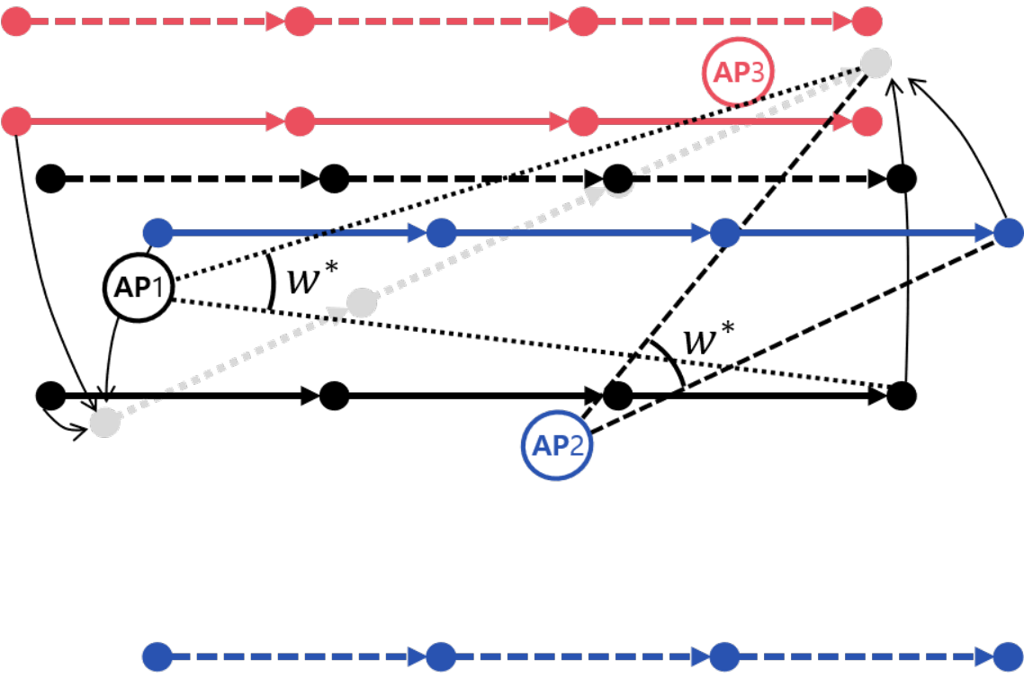

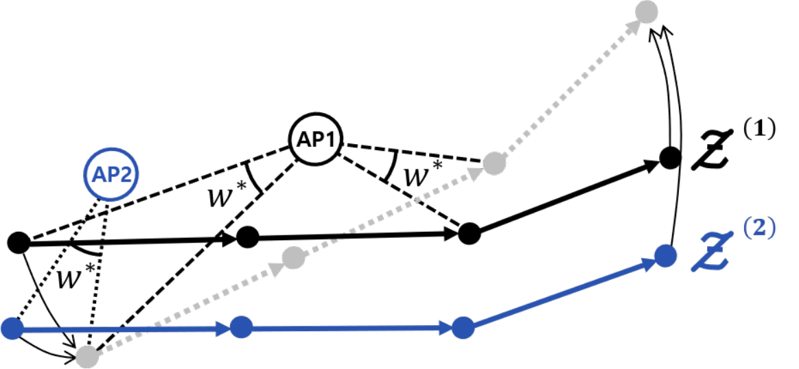

This subsection introduces the concept of TA and explains its feasible conditions. Consider the user’s relative trajectory estimated by the RTT measurements from AP , say . It is converted into a global coordinate system when the initial direction is given, namely,
| (35) |
where is AP ’s location assumed to be known in advance. Noting that the user’s location is unique regardless of which AP is used for positioning, the following condition should be met if is correctly selected, denoted by :
| (36) |
which is said that all trajectories are perfectly aligned. The aligned trajectory after TA is equivalent to the trajectory defined on the global coordinate system, denoted by , if it exists uniquely. The following proposition gives different feasible conditions of TA for linear and arbitrary mobilities.
Proposition 3 (Feasible Condition of Trajectory Alignment).
There exists a unique satisfying the condition of (36) if the number of APs not on a straight line is at least for linear mobility or the number of APs is at least for arbitrary mobility.
Proof: See Appendix A-C.
Fig. 5 and 6 respectively represent the graphical examples of TA for linear and arbitrary mobilities, showing that one more AP is required to identify whether is or . The comparison between the two from the perspective of entire procedure is discussed in the following remarks.
Remark 6 (Linear vs. Arbitrary Mobilities).
The different feasible conditions for linear mobility and arbitrary mobility stem from the difference of location dimension embedded therein. Linear mobility is interpreted as 1D location information in a 2D space, bringing about the ambiguity issue illustrated in Fig. 5. On the other hand, arbitrary mobility provides 2D location information, facilitating TA without ambiguity. This difference yields the positioning accuracy gap between the two, verified in Sec. V-A.
IV-C Algorithm Design
In an ideal case without a measurement noise, it is possible to find making all trajectories aligned perfectly, equivalent to satisfying the condition (36). In contrast, it may be challenging to do in practical cases with measurement noises, since several APs rather deteriorates the positioning accuracy if their estimation errors of bias and step length are severe. It is overcome by excluding these APs in advance and minimizing a new error function defined for TA. The detailed algorithm is explained below.
IV-C1 Feasible AP Selection
First, we aim at excluding APs unlikely to contribute to accurate positioning55 5 Our feasible AP selection is based on the assumption that RTT from all APs are measurable during walking. In the coexistence of dynamic and hotspot APs, it is required to filter them out for a reliable positioning result, like the fingerprint filtering method in [41].. To this end, we define the set of feasible APs , whose element’s bias and step length estimations, say and specified in (31) satisfy the following condition:
| (37) |
where the first and second conditions mean that the distance estimation after deducing the bias and the step length estimation should be positive, and the third condition means that the coordinates of estimated position are real numbers. The APs not in are excluded and the relative trajectories are used for the next step.


IV-C2 The Optimal Heading Direction Derivation
Depending on the mobility pattern being arbitrary or linear, different methods are used to find the optimal heading direction as follows.
Arbitrary mobility
Given , we aim at aligning all trajectories as closely as possible. Specifically, we define an error function as the sum of the Euclidean distance between two relative trajectories in , given as
By a 1D search, it is possible to find to minimize the error function , namely,
| (38) |
Linear mobility
Recall that there exists the ambiguity of relative trajectories in the case of linear mobility, say specified in (IV-A1). To remove this ambiguity, we utilize the relation between relative trajectories of different APs, as stated in the following proposition.
Proposition 4 (The Relation Between Relative Trajectories).
The distance between relative positions of two APs is always equal to the distance between the two APs, namely,
Proof: See Appendix A-D.
Select one reference AP whose index is denoted by . Depending on or , there exist two possible sequences of relative trajectories, denoted by and , initialized as and , respectively. For example, given , either C1 or C2 holds, given as
| (C1) | ||||
| (C2) |
When C1 holds (i.e., ), and are added in and , respectively. When C2 holds (i.e., ), reversely, and are added in and , respectively. The addition process is continued until . In the presence of measurement noises, neither C1 nor C2 can be satisfied. Instead, we relax C1 and C2 as and , respectively.
Given and , relative trajectories are rotated using (35), denoted by and , respectively. We define , where
By a 1D search, it is possible to find the reference AP and the corresponding to minimize the error function as
IV-C3 Determining the estimated trajectory
Last, the estimated trajectory, say , is derived by averaging as
| (39) |
V Field Experiments
This section aims at verifying the proposed positioning algorithms using several field experiments at two different indoor sites, each of which has different environments from the positioning perspective, as shown in Fig. 7. The first experimental site, called site A, is a plaza located inside the Engineering building at Yonsei University, Seoul, Korea. Site A is an open space like outdoor environments where several LOS paths exist. On the other hand, the second experimental site, called site B, is a parking lot located under Building 11 in Korea Railroad Research Institute, Uiwang, Korea. Compared with site A, most signal propagations are followed by NLOS paths due to the presence of many obstacles such as parked vehicles, walls, and pillars. The detailed experiment setups are summarized in Table II, unless specified.
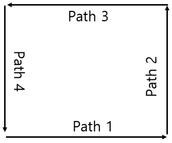
We use the algorithm in [16] to obtain the heading direction changes (see Fig. 8 as an example). As shown in Fig. 8, we consider , , , , assuming that the user’s moving direction only has finite choices depending on the surrounding arrangement (i.e., road, wall and et al.). Its effect is discussed in the sequel.
Three benchmarks are considered. The first one is based on raw RTT measurements without bias compensation for a conventional multilateration method, such as linear least square-reference selection (LLS-RS) [42]. For the second one, compensated RTT measurements are utilized for a multilateration method, but TA is not applied. The third one is an EKF-based algorithm in [20], which is operated based on and representing the scaling factors of estimated positions from PDR and WiFi, respectively. We manually optimize these parameters and set them as and . For a fair comparison, the RTT bias of each AP is compensated using our algorithm. We use the Euclidean distance of estimated positioning to ground-truth locations to represent a positioning error, i.e., .
V-A Positioning Accuracy
We verify the performance of the algorithm for the cases of linear and arbitrary mobilities. The key performance metrics are summarized in Table III.
V-A1 Linear Mobility
First, we consider the cases of linear mobility. Figure 9 illustrates a graphical example of the estimated trajectories of the proposed one and three benchmarks, while Figure 10 shows cumulative distributional functions (CDFs) of the resultant positioning errors. Several key observations are made. First, the gain of the RTT bias compensation in Sec. III is verified by comparing two benchmarks, showing significant performance improvements for both Sites A and B. Second, TA explained in Sec. IV makes all estimated points tailored to the trajectories detected by PDR, leading to additional performance enhancement. As a result, the resultant positioning errors of approximately are located within (m) and (m), and the average errors are (m) and (m) for Sites and respectively. The other performance metrics are summarized in Table III.
V-A2 Arbitrary Mobility
Second, we consider the cases of arbitrary mobility. we illustrate a graphical example of the estimated trajectories in Figure 11 and cumulative distributional functions (CDFs) of the resultant positioning errors in Figure 12, showing similar tendencies to the linear mobility counterpart. Besides, it is shown that the algorithm for arbitrary mobility provides a more accurate positioning result than that for linear mobility such that the resultant positioning errors of are approximately located within (m), (m), and (m), and the average errors are (m), (m), and (m) for Sites , , and , respectively.
It is noteworthy that the algorithm proposed for arbitrary mobility provides a more accurate positioning result than the linear mobility counterpart (see Table III). As recalled in Remark 6, arbitrary mobility embeds 2D location information, while linear mobility embeds 1D information. The difference results in a significant accuracy difference between the two.
V-A3 Comparison with EKF-based Algorithm
As shown in Figures 9, 10, 11 and 12 and Table III, we confirm that our proposed algorithm outperforms the EKF-based one for both linear and arbitrary mobility scenarios. The EKF-based algorithm updates the current position based on the previously estimated ones, resulting in accumulating errors on positioning decisions that have been already made. On the other hand, the proposed one can correct such errors by utilizing the full trajectory information.
V-B Effect of Weighed Factors and
Recall a pair of and weighting the error functions of (21) and of (26), respectively. As stated in Remark 4, the error function focuses on minimizing the error on step length and the RTT bias , while aims at minimizing the error on the initial position . Fig. 13 represents the effect of weight factors on the average positioning error, showing that provides the most accurate positioning result. It is because the errors on and can be compensated by the method of multiple combination of RSs introduced in Sec. III-D. Therefore, if a sufficient number of RSs is selected, it is optimal to focus on the minimization of .
V-C Effect of Multiple Combinations of RSs
Fig. 14 shows the average positioning error as a function of the number of candidate RSs , showing that the error is reduced from (m) to (m), when the number of RSs increases from to . On the other hand, larger than rather deteriorates a positioning result since a larger portion of RSs is likely to be severely corrupted by the measurement error. Through various simulation studies, the positioning error can be minimized in average sense by selecting the number of RSs as , where is the number of walking steps (e.g., in the experiment setting of Fig. 14) .
V-D Effect of Heading Direction Error
Recall that heading direction changes are quantized into four levels as , , , , by exploiting the prior information of surrounding arrangement. It enables us to obtain the precise trajectory estimation, as shown in Fig. 9 and 11. On the other hand, Fig. 15 plots the estimated trajectory without quantization, showing that the degradation of the positioning accuracy is marginal such that the average positioning error increases from (m) to (m) at Site A, (m) to (m) at Site B. At Site C, the positioning accuracy is slightly improved from (m) to (m). With the gyroscope error being unbiased, each error can be canceled out while moving. As a result, the entire trajectory is generally well-maintained with acceptable error, verifying the proposed algorithm to be robust against such error.
Site A Site B Site C Address Yonsei University, Korea Railroad Research Yonsei University Seoul, Korea Institute, Uiwang, Korea Seoul, Korea Type of site Indoor, plaza Underground, parking lot Indoor, conference hall Chip Intel Dual Band Qualcomm IPQ 4018 Qualcomm IPQ 4018 Wireless AC 8260 Bandwidth MHz MHz MHz Carrier GHz GHz GHz Number of WiFi APs Heights of APs m m m Heights of mobile m m m Smartphone Google Pixel XL Google Pixel XL Google Pixel XL Version Android Android Android Weight factors {0,1} {0,1} {0,1} Number of candidate RSs Linear: Linear: Arbitrary: Arbitrary: Arbitrary:
Site Mobility Number Algorithm Positioning Error (m) type of steps min max mean med std A Linear 11 w/ TA 0.705 2.459 1.359 1.269 0.570 w/ EKF 3.063 7.468 5.211 5.128 1.081 w/o TA 1.696 13.292 4.762 2.808 3.569 Raw RTT 3.95 6.874 6.064 6.365 0.835 B Linear 28 w/ TA 0.124 4.157 1.915 1.842 1.307 w/ EKF 0.703 15.196 4.496 2.612 4.249 w/o TA 0.286 14.270 3.182 2.031 3.281 Raw RTT 2.797 18.960 5.692 5.692 3.664 A Arbitrary 11 w/ TA 0.231 0.588 0.369 0.365 0.108 w/ EKF 1.290 2.422 1.956 2.071 0.358 w/o TA 1.187 3.454 2.099 1.986 0.716 Raw RTT 4.660 6.945 5.992 5.910 0.783 B Arbitrary 70 w/ TA 0.121 3.245 1.705 1.504 0.865 w/ EKF 1.947 15.115 5.243 3.773 3.510 w/o TA 0.976 21.092 5.963 4.015 4.866 Raw RTT 0.218 15.727 5.525 4.653 3.555 C Arbitrary 70 w/ TA 0.046 1.715 0.978 1.014 0.407 w/ EKF 1.064 7.406 4.199 4.064 1.397 w/o TA 0.857 14.439 4.743 3.095 3.072 Raw RTT 1.064 7.406 4.199 4.064 1.397
VI Concluding Remark
This work has presented a novel positioning algorithm to estimate a user’s location by integrating RTT and PDR measurements. Geometric relations between the two are formulated as mathematical form, enabling us to design a tractable and scalable positioning algorithm as well as provide the feasible conditions of the number of steps and WiFi APs for a unique positioning. The superiority of the proposed method has been well verified by field experiments that the positioning accuracy can be significantly improved than the conventional multilateration techniques.
The current work can be extended in several directions. First, our algorithm can help simultaneous localization and mapping (SLAM) by identifying whether a blockage exists from the concerned AP from the corresponding RTT bias. Second, our algorithm can be applied to the area of vehicle and drone positioning [43] that has not been actively explored yet. Last, it is interesting to integrate such a sensing system into a wireless communication system using several techniques, e.g., compressive sensing [44] and over-the-air computation [45], a key direction in B5G/6G communications.
Appendix A Appendix
A-A Verifying Effect of Deterministic Bias Assumption
This subsection aim at verifying that our algorithm can reduce the error due to the deterministic bias in Assumption 1 as marginal using RS selection and multiple combinations of RSs.
- •
Reference Step Selection: Recall that when making the systems of linear equations in E1 and E2, two RSs play a pivotal role in the linearization process (see Sec. III-B and Sec. III-C). In other words, with the RSs whose biases violate Assumption 1, their effects propagate throughout the entire equations, causing severe errors on the resulting solution. It is thus required to select RSs with biases being relatively constant. Fig. 17 plots the variations of RTT and bias during the full-trajectory in Site B, showing that the biases within a specific range are relatively constant when the corresponding RTTs are small. As a result, we select two RSs whose RTTs are smaller. Compared with selecting RSs randomly, selecting two RSs having the smallest RTT can reduce the average error on step length estimation up to (m).
- •
Multiple Combinations of Reference Steps: Fig. 18(a) represents the estimated step length from two RSs sorted by RTT measurements; A smaller index represents that the sum of the selected RSs’ RTTs is smaller. It is observed that smaller RTT does not always provide a higher estimation accuracy. To cope with this issue, several candidate RSs are selected instead of a single pair (See Sec. III-D). Fig. 17 shows that the standard deviation of candidate RSs’ RTTs is significantly smaller than that of all RTTs, validating the deterministic bias assumption in Assumption 1. It leads to providing a reliable step-length estimation for all APs as shown in Fig. 18(b).
A-B Proof of Proposition 2
Noting that E2 has equations, it is an overdetermined system when if the rank of the matrix in (III-C) is . Then, there always exists satisfying since E2 is formulated from a geometric representation of multiple unknowns.
Consider a special case of where . At this case, because if , and by definition. From this, the matrix components and can be changed as
| (40) |
| (41) |
Above (A-B) and (A-B) have common terms , the matrix which defined as (III-C) becomes
| (42) |
Therefore, the rank of is 1, it is underdetermined system. This finishes the proof.
A-C Proof of Proposition 3
We provide separated proofs for arbitrary and linear mobilities.
A-C1 Arbitrary mobility
Consider the case with APs and . Using (35), a pair of relative locations at , say and , are given as
| (43) | |||
| (44) |
where is a rotation matrix. Their relation is derived by subtracting the above two as
| (45) |
Noting that if , the above is reduced as
| (46) |
where is unique since the rotation matrix is not ambiguous between . Next, the relation between two relative locations at , say and , is given as
| (47) | ||||
| (48) |
The above is straightforwardly extended into other relative locations at . In other words, two relative trajectories and , are perfectly aligned when . We complete the proof.
A-C2 Linear Mobility


Consider the case with APs , , and . Recall that there are two relative trajectories for each AP, say . Following the same step in the arbitrary mobility counterpart, two possible global coordinates are made for APs and , denoted by and , which are symmetric concerning the line between the locations of APs and (See Fig. 19). Specifically, the corresponding heading directions, denoted by and , has the following geometric relation as
| (49) |
where returns the angle of the vector . Between the two, one is real whereas the other is fake. Similarly, the resultant heading directions for APs and , denoted by and , gives
| (50) |
Using the above two equations, it is easy to identify which ones are real. For example, assume and are real, namely, . Unless , it is obvious to identify and are fake since they are different. Note that if all APs exist on a straight line, it cannot be distingished between real and fake ones because symmetry is maintained, completing the proof.
A-D Proof of Proposition 4
References
- [1] A. Bensky, Wireless positioning technologies and applications, second edition. Artech House, 2016.
- [2] C. Laoudias, A. Moreira, S. Kim, S. Lee, L. Wirola, and C. Fischione, “A survey of enabling technologies for network localization, tracking, and navigation,” IEEE Commun. Surveys Tuts., vol. 20, no. 4, pp. 3607–3644, Fourthquarter 2018.
- [3] C. Yang and H.-R. Shao, “Wifi-based indoor positioning,” IEEE Commun. Mag., vol. 53, no. 3, pp. 150–157, Mar. 2015.
- [4] T. D. Vy, T. L. Nguyen, and Y. Shin, “A smartphone indoor localization using inertial sensors and single wi-fi access point,” in Proc. Int. Conf. Indoor Positioning Indoor Navigat. (IPIN). IEEE, Sep. 2019, pp. 1–7.
- [5] IEEE Standard for Information Technology–Telecommunications and Information Exchange Between Systems Local and Metropolitan Area Networks–Specific Requirements - Part 11: Wireless LAN medium access control (MAC) and physical layer (PHY) specification, IEEE Standard 802.11-2016 (Revision of IEEE Standard 802.11-2012), Dec. 2016.
- [6] L. Banin, O. Bar-Shalom, N. Dvorecki, and Y. Amizur, “High-accuracy indoor geolocation using collaborative time of arrival (CToA),” Intel White Paper, pp. 1–14, Sep. 2017.
- [7] M. Ibrahim, H. Liu, M. Jawahar, V. Nguyen, M. Gruteser, R. Howard, B. Yu, and F. Bai, “Verification: accuracy evaluation of WiFi fine time measurements on an open platform,” in Proc. 24th Annu. Int. Conf. Mobile Comput. Netw. (MobiCom), Nov. 2018, pp. 417–427.
- [8] M. Si, Y. Wang, S. Xu, M. Sun, and H. Cao, “A Wi-Fi FTM-based indoor positioning method with LOS/NLOS identification,” Appl. Sci., vol. 10, no. 3, p. 956, 2020.
- [9] K. Han, S. M. Yu, and S.-L. Kim, “Smartphone-based indoor localization using wi-fi fine timing measurement,” in Proc. Int. Conf. Indoor Positioning Indoor Navigat. (IPIN), Sep. 2019, pp. 1–5.
- [10] K. Bregar and M. Mohorcic, “Improving indoor localization using convolutional neural networks on computationally restricted devices,” IEEE Access, vol. 6, pp. 17 429–17 441, 2018.
- [11] J. Choi, Y. S. Choi, and S. Talwar, “Unsupervised learning techniques for trilateration: From theory to android app implementation,” IEEE Access, vol. 7, pp. 134 525–134 538, 2019.
- [12] R. Toledo-Moreo, D. Bétaille, F. Peyret, and J. Laneurit, “Fusing GNSS, dead-reckoning, and enhanced maps for road vehicle lane-level navigation,” IEEE J. Sel. Topics Signal Process., vol. 3, no. 5, pp. 798–809, Oct. 2009.
- [13] Z. Yang, C. Wu, Z. Zhou, X. Zhang, X. Wang, and Y. Liu, “Mobility increases localizability: a survey on wireless indoor localization using inertial sensors,” ACM Comput. Surveys, vol. 47, no. 3, pp. 54:1–54:34, Apr. 2015.
- [14] M. H. Afzal, V. Renaudin, and G. Lachapelle, “Magnetic field based heading estimation for pedestrian navigation environments,” Proc. Int. Conf. Indoor Positioning Indoor Navigat. (IPIN), pp. 1–10, 2011.
- [15] H. Weinberg, “Using the ADXL202 in pedometer and personal navigation applications,” Application Notes American Devices, 2002. [Online]. Available: http://application-notes.digchip.com/013/13-14984.pdf
- [16] W. Kang and Y. Han, “SmartPDR: Smartphone-based pedestrian dead reckoning for indoor localization,” IEEE Sensors J., vol. 15, no. 5, pp. 2906–2916, May 2015.
- [17] B. M. Scherzinger, “Inertial navigator error models for large heading uncertainty,” in Proc. Position Location Navigat. Symp. (PLANS), 1996, pp. 477–484.
- [18] X. Guo, N. Ansari, F. Hu, Y. Shao, N. R. Elikplim, and L. Li, “A survey on fusion-based indoor positioning,” IEEE Commun. Surveys Tuts., vol. 22, no. 1, pp. 566–594, Firstquarter 2020.
- [19] J. Choi and Y.-S. Choi, “Calibration-free positioning technique using Wi-Fi ranging and built-in sensors of mobile devices,” IEEE Internet of Things J., vol. 8, no. 1, pp. 541–554, Jan. 2021.
- [20] M. Sun, Y. Wang, S. Xu, H. Qi, and X. Hu, “Indoor positioning tightly coupled Wi-Fi FTM ranging and PDR based on the extended kalman filter for smartphones,” IEEE Access, vol. 8, pp. 49 671–49 684, 2020.
- [21] Y. Yu, R. Chen, L. Chen, S. Xu, W. Li, Y. Wu, and H. Zhou, “Precise 3-D indoor localization based on Wi-Fi FTM and built-in sensors,” IEEE Internet of Things J., vol. 7, no. 12, pp. 11 753–11 765, Dec. 2021.
- [22] X. Liu, B. Zhou, P. Huang, W. Xue, Q. Li, J. Zhu, and L. Qiu, “Kalman filter-based data fusion of Wi-Fi RTT and PDR for indoor localization,” IEEE Sensors J., vol. 21, no. 6, pp. 8479–8490, Mar. 2021.
- [23] L. Banin, P. Tikva, U. Schatzberg, P. Tikva, and P. Tikva, “WiFi FTM and map information fusion for accurate positioning,” in Proc. Int. Conf. Indoor Positioning Indoor Navigat. (IPIN), Oct. 2016, pp. 1–4.
- [24] C. H. Hsieh, J. Y. Chen, and B. H. Nien, “Deep learning-based indoor localization using received signal strength and channel state information,” IEEE Access, vol. 7, pp. 33 256–33 267, 2019.
- [25] J. Choi, “Sensor-aided learning for Wi-Fi positioning with beacon channel state information,” arXiv:2007.06204, 2020.
- [26] S. Xu, R. Chen, Y. Yu, G. Guo, and L. Huang, “Locating smartphones indoors using built-in sensors and Wi-Fi ranging with an enhanced particle filter,” IEEE Access, vol. 7, pp. 95 140–95 153, 2019.
- [27] H. Miao, K. Yu, and M. J. Juntti, “Positioning for NLOS propagation: Algorithm derivations and Cramer-Rao bounds,” IEEE Trans. Veh. Technol., vol. 56, no. 5, pp. 2568–2580, Sep. 2007.
- [28] A. Frischen, J. Hasch, and C. Waldschmidt, “A cooperative MIMO radar network using highly integrated FMCW radar sensors,” IEEE Trans. Microw. Theory Techn., vol. 65, no. 4, pp. 1355–1366, Apr. 2017.
- [29] K. Han, S. W. Ko, H. Chae, B. H. Kim, and K. Huang, “Hidden vehicle sensing via asynchronous V2V transmission: A multi-path-geometry approach,” IEEE Access, vol. 7, pp. 169 399–169 416, 2019.
- [30] A. Malyugina, K. Igudesman, and D. Chickrin, “Least-squares fitting of a three-dimensional ellipsoid to noisy data,” Appl. Math. Sci., vol. 8, no. 149, pp. 7409–7421, 2014.
- [31] J. F. Vasconcelos, G. Elkaim, C. Silvestre, P. Oliveira, and B. Cardeira, “Geometric approach to strapdown magnetometer calibration in sensor frame,” IEEE Trans. Aerosp. Electron. Syst., vol. 47, no. 2, pp. 1293–1306, Apr. 2011.
- [32] B. Wang, X. Liu, B. Yu, R. Jia, and X. Gan, “Pedestrian dead reckoning based on motion mode recognition using a smartphone,” Sensors, vol. 18, no. 6, p. 1811, 2018.
- [33] J. S. Lee and S. M. Huang, “An experimental heuristic approach to multi-pose pedestrian dead reckoning without using magnetometers for indoor localization,” IEEE Sensors J., vol. 19, no. 20, pp. 9532–9542, Oct. 2019.
- [34] O. P. Jasuja, S. Harbhajan, and K. Anupama, “Estimation of stature from stride length while walking fast,” Forensic Sci. Int., vol. 86, no. 3, pp. 181–186, 1997.
- [35] H. B. Menz, S. R. Lord, and R. C. Fitzpatrick, “Age-related differences in walking stability,” Age and Ageing, vol. 32, no. 2, pp. 137–142, 2003.
- [36] I. Bisio, F. Lavagetto, M. Marchese, and A. Sciarrone, “Smartphone-based user activity recognition method for health remote monitoring applications,” in Proc. Int. Conf. Pervasive and Embedded Comput. Commun. Systems (PECCS), Feb. 2012.
- [37] B. Zhou, J. Yang, and Q. Li, “Smartphone-based activity recognition for indoor localization using a convolutional neural network,” Sensors, vol. 19, no. 3, p. 621, 2019.
- [38] B. K. Horn, “Doubling the accuracy of indoor positioning: Frequency diversity,” Sensors, vol. 20, p. 1489, 2020.
- [39] R. Casas, A. Marco, J. J. Guerrero, and J. Falcó, “Robust estimator for non-line-of-sight error mitigation in indoor localization,” EURASIP J. Adv. Signal Process., vol. 2006, 2006.
- [40] T. Qiao and H. Liu, “Improved least median of squares localization for non-line-of-sight mitigation,” IEEE Commun. Lett., vol. 18, no. 8, pp. 1451–1454, Aug. 2014.
- [41] I. Bisio, C. Garibotto, F. Lavagetto, and A. Sciarrone, “Outdoor places of interest recognition with WiFi fingerprint over mobile devices,” in IEEE Int. Conf. Coommun. (ICC), May 2019, pp. 1–7.
- [42] I. Guvenc, S. Gezici, F. Watanabe, and H. Inamura, “Enhancements to linear least squares localization through reference selection and ML estimation,” in Proc. IEEE Wireless Commun. Netw. Conf. (WCNC), 2008, pp. 284–289.
- [43] S. W. Ko, H. Chae, K. Han, S. Lee, and K. Huang, “V2X-based vehicular positioning: Opportunities, challenges, and future directions,” IEEE Wireless Commun., Early access, 2021.
- [44] C. Han, L. Chen, and W. Wang, “Compressive sensing in wireless powered network: regarding transmission as measurement,” IEEE Wireless Commun. Letters, vol. 8, no. 6, pp. 1709–1712, Dec. 2019.
- [45] L. Chen, N. Zhao, Y. Chen, F. R. Yu, and G. Wei, “Over-the-air computation for cooperative wideband spectrum sensing and performance analysis,” IEEE Trans. Veh. Technol., vol. 67, no. 11, pp. 10 603–10 614, Nov. 2018.
![[Uncaptioned image]](2011.03698v2/Bio/KyuwonHan.jpg) |
Kyuwon Han (S’21) received the B.S degrees in physics from Chung-Ang University, South Korea in 2018. He is currently a Ph.D student in Electrical and Electronic Engineering at Yonsei University, South Korea. His research interests include indoor positioning, spectrum sharing, and machine learning techniques for wireless communications. Mr. Han received a bronze prize at IEEE Seoul Section Student Papar Award in 2019. |
![[Uncaptioned image]](2011.03698v2/Bio/SeungMinYu.jpg) |
Seung Min Yu received the B.S. (Hons.) and Ph.D. degrees in electrical and electronic engineering from Yonsei University, South Korea, in 2009 and 2013, respectively. He is currently a Senior Researcher with the Korea Railroad Research Institute, South Korea. He was a Senior Engineer with Networks Business, Samsung Electronics Company, Ltd., South Korea. He was also a Researcher with the Internet Research Division, NAVER Corporation (South Korea’s most popular search engine), South Korea. His research interests include indoor positioning, optimization for wireless networks, and economics of wireless systems. Dr. Yu received the Student Travel Grant Award at the IEEE Global Communications Conference in 2011 and the Best Paper Award at the IEEE Vehicular Technology Conference in 2013. |
![[Uncaptioned image]](2011.03698v2/Bio/Seung-LyunKim.jpg) |
Seung-Lyun Kim is a Professor and Head of the School of Electrical & Electronic Engineering, Yonsei University, Seoul, Korea, heading the Robotic & Mobile Networks Laboratory (RAMO) and the Center for Flexible Radio (CFR+). He is co-directing H2020 EUK PriMO-5G project, and leading Smart Factory Committee of 5G Forum, Korea. He was an Assistant Professor of Radio Communication Systems at the Department of Signals, Sensors & Systems, Royal Institute of Technology (KTH), Stockholm, Sweden. He was a Visiting Professor at the Control Engineering Group, Helsinki University of Technology (now Aalto), Finland, the KTH Center for Wireless Systems, and the Graduate School of Informatics, Kyoto University, Japan. He served as a technical committee member or a chair for various conferences, and an editorial board member of IEEE Transactions on Vehicular Technology, IEEE Communications Letters, Elsevier Control Engineering Practice, Elsevier ICT Express, and Journal of Communications and Network. He served as the leading guest editor of IEEE Wireless Communications and IEEE Network for wireless communications in networked robotics, and IEEE Journal on Selected Areas in Communications. He also consulted various companies in the area of wireless systems both in Korea and abroad. His research interest includes radio resource management, information theory in wireless networks, collective intelligence, and robotic networks. He published numerous papers, including the co-authored book (with Prof. Jens Zander), Radio Resource Management for Wireless Networks. His degrees include BS in economics (Seoul National University), and MS & PhD in operations research (with application to wireless networks, Korea Advanced Institute of Science & Technology). |
![[Uncaptioned image]](2011.03698v2/Bio/Seung-WooKo.jpg) |
Seung-Woo Ko (M’17) received the B.S., M.S., and Ph.D. degrees from the School of Electrical and Electronic Engineering, Yonsei University, South Korea, in 2006, 2007, and 2013, respectively. Since March 2019, he has been an Assistant Professor with the Division of Electronics and Electrical Information Engineering, Korea Maritime and Ocean University (KMOU). Before joining KMOU, he has been a Senior Researcher with LG Electronics, South Korea, from March 2013 to June 2014, and a Postdoctoral Researcher at Yonsei University, South Korea, from July 2014 to March 2016, and The University of Hong Kong, from April 2016 to February 2019. His research interests focus on intelligent wireless communications and networking, with special emphasis on edge computing and learning, vehicular technologies, and localization. |