In many survey data settings, there is dependence between a unit’s probability of selection and the response of interest. This is termed informative sampling and is known to introduce bias into the model when ignored. Thus, in survey data settings, it is important to account for the survey design in some manner in order to eliminate or reduce this bias. In other words, complex sample designs can lead to samples that are unrepresenative of the population and, thus, the sample model should be adjusted in some way to account for this.

Parker et al., 2019 give an overview of various methods to account for informative sampling. Of primary interest is the pseudo-likelihood (PL) method introduced by Skinner, 1989 and Binder, 1983. This approach adjusts the likelihood function by exponentially weighting each unit’s likelihood contribution by the corresponding survey weight (i.e. the inverse of the selection probability),

$$\prod_{i\in\mathcal{S}}f(y_{i}\mid\bm{\theta})^{w_{i}},$$

(1)

where $\mathcal{S}$ indicates the sample, $y_{i}$ represents the response value for unit $i$ with survey weight $w_{i}$. In a frequentist setting, this PL can be maximized to give a point estimate for $\bm{\theta},$ however more complex procedures are necessary to give appropriate estimates of uncertainty.

Savitsky and Toth, 2016 show that a PL may also be used in a Bayesian framework. In particular, they show that under informative sampling, the use of a PL along with a prior specification leads to a pseduo-posterior distribution,

$$\hat{\pi}(\bm{\theta}|\mathbf{y},\mathbf{\tilde{w}})\propto\left\{\prod_{i\in\mathcal{S}}f(y_{i}|\bm{\theta})^{\tilde{w}_{i}}\right\}\pi(\bm{\theta}),$$

that converges to the population posterior distribution. In this scenario, it is important to scale the weights to sum to the sample size in order to attain the appropriate estimates of uncertainty. These scaled weights are represented by $\tilde{w}_{i}.$ This formulation applies generally to Bayesian models and is the approach we use herein to account for informative sampling.

Modeling non-Gaussian data types in a Bayesian setting can be computationally burdensome, especially while accounting for informative sampling. Parker et al., 2020 utilize a data augmentation approach to construct a flexible mixed model for Binomial and Multinomial data under informative sampling. Their model for Binomial data is given by,

$$\begin{split}\bm{Z}|\bm{\beta,\eta}&\propto\prod_{i\in S}\hbox{Bin}\left(Z_{i}|n_{i},p_{i}\right)^{\stackrel{{\scriptstyle\sim}}{{w}}_{i}}\\ \hbox{logit}(p_{i})&=\bm{x}_{i}^{\prime}\bm{\beta}+\bm{\phi}_{i}^{\prime}\bm{\eta}\\ \bm{\eta}|\sigma^{2}_{\eta}&\sim\hbox{N}_{r}(\bm{0_{r}},\sigma_{\eta}^{2}\bm{I}_{r})\\ \bm{\beta}&\sim\hbox{N}_{q}(\bm{0_{q}},\sigma_{\beta}^{2}\bm{I}_{q})\\ \sigma_{\eta}^{2}&\sim\hbox{IG}(a,b)\\ &\sigma_{\beta},a,b>0,\end{split}$$

(2)

where $Z_{i}$ represents the response value for unit $i$ in the sample. In this case, $\bm{x}_{i}$ is a vector of fixed effects covariates and $\bm{\phi}_{i}$ represents a set of spatial basis functions.

In order to fit this model in a computationally efficient manner, Pólya-Gamma data augmentation is used. Specifically, letting $\hbox{PG}(\cdot,\cdot)$ represent a Pólya-Gamma distribution, Polson et al., 2013 show that

$$\frac{(e^{\psi})^{a}}{(1+e^{\psi})^{b}}=2^{-b}e^{\kappa\psi}\int_{0}^{\infty}e^{-\omega\psi^{2}/2}p(\omega)d\omega,$$

where $\kappa=a-b/2$ and $p(\omega)$ is a $\hbox{PG}(b,0)$ density. They further show that $(\omega|\psi)\sim\hbox{PG}(b,\psi)$. The PL in (2) can be written,

$$\prod_{i\in\mathcal{S}}\left(\frac{(e^{\psi_{i}})^{Z_{i}}}{(1+e^{\psi_{i}})^{n_{i}}}\right)^{\tilde{w}_{i}}=\prod_{i\in\mathcal{S}}\frac{(e^{\psi_{i}})^{Z_{i}^{*}}}{(1+e^{\psi_{i}})^{n_{i}^{*}}},$$

where $\psi_{i}=\hbox{logit}(p_{i}),$ $Z_{i}^{*}=Z_{i}\times\tilde{w}_{i},$ and $n_{i}^{*}=n_{i}\times\tilde{w}_{i}$. This allows for data augmentation of a latent Pólya-Gamma random variable that leads to conjugate Normal priors on the regression parameters.

The Binomial model in (2) can also be extended to Multinomial or Categorical data. Following Linderman et al., 2015, the Multinomial distribution with $C$ categories can be rewritten as

$$\begin{split}\hbox{Multinomial}(\bm{Z}|n,\bm{p})=\prod_{c=1}^{C-1}\hbox{Bin}(Z_{c}|n_{c},\tilde{p}_{c}),\end{split}$$

where

$$n_{c}=n-\sum_{j<c}Z_{j},\;\;\tilde{p}_{c}=\frac{p_{c}}{1-\sum_{j<c}p_{j}},\;\;c=2,\ldots,C.$$

In this light, a series of $C-1$ Binomial models may be fit to estimate the parameters for a Multinomial data model.

The modeling framework of Parker et al., 2020 is useful for fitting Binomial data under informative sampling, such as the NHANES mortality data of interest; however, the approach must be extended in order to consider functional covariates.

Consider the case where we have $J$ functional covariates and $\kappa_{ij}(t),t\in\mathcal{T}$ denotes the $j$th functional covariate ($j=1,\ldots,J$) for unit $i$ at time $t.$ In our case, the domain is time, though other domains may be appropriate depending on the type of functional data. Then, (2) can be extended for functional covariates by letting

$$\hbox{logit}(p_{i})=\bm{x}_{i}^{\prime}\bm{\beta}+\sum_{j=1}^{J}\int_{\mathcal{T}}\eta_{j}(t)\kappa_{ij}(t)dt,$$

where $\eta_{j}(t)$ is a functional regression parameter associated with functional covariate $j.$ In what follows, we will assume $J=1$ (and drop the subscript $j$), as is the case in our example, but we note that the approach is still applicable for $J>1.$

In order to reduce the dimension of the problem, we can use a basis expansion representation. In particular, let $\left\{\phi_{k}(t):k=1,2,\ldots\right\}$ be a complete orthonormal basis of the domain $\mathcal{T}.$ Then, we can represent the functional covariate as

$$\kappa_{i}(t)=\sum_{k=1}^{\infty}\xi_{i}(k)\phi_{k}(t)$$

and

$$\eta(t)=\sum_{k=1}^{\infty}b(k)\phi_{k}(t),$$

where $\xi_{i}(k)$ and $b(k)$ are the expansion coefficients for $\kappa_{i}(\cdot)$ and $\eta(\cdot)$ respectively. Now, appealing to orthonormality,

$$\hbox{logit}(p_{i})=\bm{x}_{i}^{\prime}\bm{\beta}+\int_{\mathcal{T}}\eta(t)\kappa_{i}(t)dt=\bm{x}_{i}^{\prime}\bm{\beta}+\sum_{k=1}^{\infty}b(k)\xi_{i}(k).$$

(3)

Note that any orthonormal basis may be used here, though we use functional principal components selected through the fast covariance estimation (FAST) approach (Xiao et al., 2016). This is easily implemented via the use of the refund package in R (Goldsmith et al., 2019).

In practice, the summation in (3) is truncated to $K$. For our purposes, we truncate the summation (i.e., choose K) such that the retained components explain 95% of the variation in the functional data. This results in a finite, though potentially large, number of basis functions. Furthermore, any given basis function may not necessarily be related to the response. Thus, we require some form of variable selection and shrinkage estimator. By doing so, the variable selection prior is able to determine which components of the variation in functional data are correlated with the response. This is similar to the approach taken by Holan et al., 2010.

In order to provide shrinkage to our functional regression coefficients, we utilize the Horsehoe prior introduced by Carvalho et al., 2010. Although many other methods of Bayesian variable selection exist, this has the advantage of being fully specified, without requiring hyperparameter selection, as well as providing minimial shrinkage to strong signals while still providing a high degree of shrinkage for noise. To implement the Horsehoe prior for (3), we use the following hierarchy,

	$\displaystyle b(k)|\lambda_{k},\tau$	$\displaystyle\stackrel{{\scriptstyle ind}}{{\sim}}\hbox{N}(0,\lambda_{k}^{2}\tau^{2}),\;k=1,\ldots,K$
	$\displaystyle\lambda_{k}$	$\displaystyle\stackrel{{\scriptstyle ind}}{{\sim}}\hbox{C}^{+}(0,1)$
	$\displaystyle\tau$	$\displaystyle\sim\hbox{C}^{+}(0,1),$

where $\hbox{C}^{+}(\cdot,\cdot)$ represents the Cauchy density truncated below at zero. This prior is considered a global-local shrinkage approach. This can be seen by recognizing that $\tau$ applies to all regression parameters and determines the overall level of shrinkage, whereas $\lambda_{k}$ is local and applies to a specific coefficient. In this way, coefficients corresponding to noise can attain a higher degree of shrinkage than those with strong signals.

The half-Cauchy priors used in the Horsehoe are not conjugate. However, Makalic and Schmidt, 2015 use a data augmentation approach to allow for Gibbs sampling within the Horshoe prior framework. In particular,they use a scale mixture representation of the half-Cauchy such that when $x\sim\hbox{C}^{+}(0,A)$, then $x^{2}|a\sim\hbox{IG}(1/2,1/a)$ and $a\sim\hbox{IG}(1/2,1/A^{2}),$ where $\hbox{IG}(a,b)$ represents the Inverse Gamma distribution with shape parameter $a$ and scale parameter $b.$ This leads to an alternate formulation of the Horsehoe prior hierarchy,

	$\displaystyle b(k)|\lambda_{k},\tau$	$\displaystyle\stackrel{{\scriptstyle ind}}{{\sim}}\hbox{N}(0,\lambda_{k}^{2}\tau^{2}),\;k=1,\ldots,K$
	$\displaystyle\lambda_{k}^{2}|\nu_{k}$	$\displaystyle\stackrel{{\scriptstyle ind}}{{\sim}}\hbox{IG}(1/2,1/\nu_{k})$
	$\displaystyle\tau^{2}|\nu_{\tau}$	$\displaystyle\sim\hbox{IG}(1/2,1/\nu_{\tau})$
	$\displaystyle\nu_{1},\ldots,\nu_{K},\nu_{\tau}$	$\displaystyle\stackrel{{\scriptstyle ind}}{{\sim}}\hbox{IG}(1/2,1),$

that allows for straightforward Gibbs sampling.

We now present our model for non-Gaussian data under informative sampling with functional covariates, which makes use of the modeling elements discussed so far:

$$\begin{split}\bm{Z}|\bm{\beta,\eta}&\propto\prod_{i\in S}\hbox{Bin}\left(Z_{i}|n_{i},p_{i}\right)^{\stackrel{{\scriptstyle\sim}}{{w}}_{i}}\\ \hbox{logit}(p_{i})&=\bm{x}_{i}^{\prime}\bm{\beta}+\sum_{k=1}^{K}b(k)\xi_{i}(k)\\ \bm{\beta}&\sim\hbox{N}_{q}(\bm{0_{q}},\sigma_{\beta}^{2}\bm{I}_{q})\\ b(k)|\lambda_{k},\tau&\stackrel{{\scriptstyle ind}}{{\sim}}\hbox{N}(0,\lambda_{k}^{2}\tau^{2}),\;k=1,\ldots,K\\ \lambda_{k}^{2}|\nu_{k}&\stackrel{{\scriptstyle ind}}{{\sim}}\hbox{IG}(1/2,1/\nu_{k})\\ \tau^{2}|\nu_{\tau}&\sim\hbox{IG}(1/2,1/\nu_{\tau})\\ \nu_{1},\ldots,\nu_{K},\nu_{\tau}&\stackrel{{\scriptstyle ind}}{{\sim}}\hbox{IG}(1/2,1)\\ &\sigma_{\beta}^{2}>0.\end{split}$$

(4)

In this model, $\bm{x}_{i}$ represents a $q$-dimensional vector of scalar covariates and $\xi_{i}(k)$ represents the $k$th basis expansion coefficient for observation $i.$

This model makes use of a Bayesian pseudo-likelihood to account for informative sampling, allowing for population level inference. We also make use of Pólya-Gamma data augmentation for efficient Gibbs sampling. If desired, prior information on the scalar covariates may be incorporated through the selection of $\sigma^{2}_{\beta},$ though we use a relatively diffuse prior by letting $\sigma^{2}_{\beta}=10.$ The full conditional distributions are given in the Appendix.

It is straightforward to implement the model in the Multinomial data setting through the use of a stick-breaking representation, as discussed in Section 2.2. It would also be straightforward to use a Gaussian pseudo-likelihood in place of the Binomial one given here, as conjugacy would be retained.

Using our Bayesian pseudo-likelihood based model for functional covariates (FM-W), we now analyze the NHANES PAM data and its relationship with mortality. We use the same dataset considered in the simulation study and outlined in Section 3, with a sample size of 3,208. We treat the 5-year mortality indicator as our binary response, and use an intercept and age as our scalar covariates as well as the PAM data as a functional covariate. We use the FACE functional principal components basis representation and retain the first 19 components, explaining 95% of the variation in the functional data.

We fit the model via Gibbs sampling with 5,000 iterations and discard the first 1,000 iterations as burn-in. Convergence was assessed via traceplots of the sample chains, where no lack of convergence was detected.

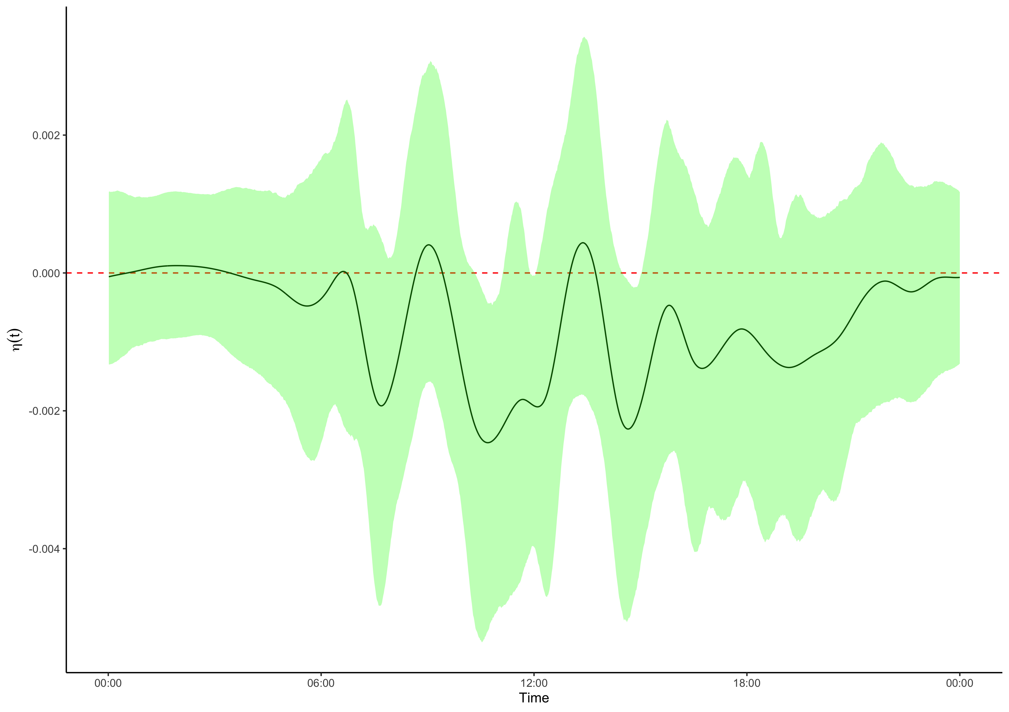
After fitting the model, we are able to make population level inference. We plot the posterior mean of the functional regression coefficient, $\eta(t)$, along with a pointwise 90% credible interval in Figure 2. For the most part the $\eta(t)$ is estimated to be negative, as expected, indicating that increased levels of activity are associated with lower expected mortality rate. There are two primary time periods where the credible interval does not contain zero, around 10 a.m. to 12 p.m. and around 2 p.m. to 3 p.m.

In addition to examination of the functional regression coefficient, we can also glean insight by examining how variation in activity level of individuals changes mortality estimates. In Figure 3, we plot activity curves for 3 hypothetical individuals all age 65 along with the accompanying posterior distribution of 5-year mortality rate. Individual A has a very low level of activity, resulting in a high expected mortality rate. However, there is also a great deal of uncertainty around this rate. Individuals B and C both have increasing level of overall activity, especially in the early morning and late afternoon, resulting in decreasing expected mortality rate. As the activity level increases, the uncertainty around the mortality rate decreases.

In addition to univariate estimation, our model allows for multivariate estimation through the Multinomial data model. In this case we wish to make joint mortality estimates for years 1-5. To do so, we begin by assigning survey respondents into distinct categories: those who died within one year of the survey, those who died after 1 year but before 2 years, those who died after 2 years but before 3 years, those who died after 3 years but before 4 years, those who died after 4 years but before 5 years, and finally those that did not die before 5 years. Assigning groups in this way results in a Multinomial or Categorical data distribution with 6 categories. Thus, we are able to use the stick breaking representation of the Multinomial distribution in order to fit $C-1=5$ independent Binomial data models that allow us to make joint estimates of mortality at various time points.

We use the same hypothetical individuals from our 5-year mortality example to examine the effects of activity level on multi-year mortality. Figure 4 plots the activity curves for these individuals alongside their posterior mean mortality rates for year 1-5. We also provide 90% credible intervals. Once again, we see that both expected mortality rate and uncertainty increase as activity level generally decreases. Because these estimates are multivariate, we can also see that decreased activity is associated with steeper marginal increases in mortality for the near future than for years further away from the survey.

References

- Binder, (1983) Binder, D. A. (1983). “On the variances of asymptotically normal estimators from complex surveys.” International Statistical Review, 51, 3, 279–292.
- Brewer et al., (1984) Brewer, K., Early, L., and Hanif, M. (1984). “Poisson, modified Poisson and collocated sampling.” Journal of Statistical Planning and Inference, 10, 1, 15–30.
- Carvalho et al., (2010) Carvalho, C. M., Polson, N. G., and Scott, J. G. (2010). “The horseshoe estimator for sparse signals.” Biometrika, 97, 2, 465–480.
- Goldsmith et al., (2019) Goldsmith, J., Scheipl, F., Huang, L., Wrobel, J., Di, C., Gellar, J., Harezlak, J., McLean, M. W., Swihart, B., Xiao, L., Crainiceanu, C., and Reiss, P. T. (2019). refund: Regression with Functional Data. R package version 0.1-21.
- Holan et al., (2010) Holan, S. H., Wikle, C. K., Sullivan-Beckers, L. E., and Cocroft, R. B. (2010). “Modeling complex phenotypes: generalized linear models using spectrogram predictors of animal communication signals.” Biometrics, 66, 3, 914–924.
- Leroux et al., (2019) Leroux, A., Di, J., Smirnova, E., Mcguffey, E. J., Cao, Q., Bayatmokhtari, E., Tabacu, L., Zipunnikov, V., Urbanek, J. K., and Crainiceanu, C. (2019). “Organizing and analyzing the activity data in nhanes.” Statistics in Biosciences, 11, 2, 262–287.
- Linderman et al., (2015) Linderman, S., Johnson, M. J., and Adams, R. P. (2015). “Dependent multinomial models made easy: Stick-breaking with the Pólya-Gamma augmentation.” In Advances in Neural Information Processing Systems, 3456–3464.
- Makalic and Schmidt, (2015) Makalic, E. and Schmidt, D. F. (2015). “A simple sampler for the horseshoe estimator.” IEEE Signal Processing Letters, 23, 1, 179–182.
- Parker et al., (2020) Parker, P. A., Holan, S. H., and Janicki, R. (2020). “Computationally Efficient Bayesian Unit-Level Models for Non-Gaussian Data Under Informative Sampling.” arXiv preprint arXiv:2009.05642.
- Parker et al., (2019) Parker, P. A., Janicki, R., and Holan, S. H. (2019). “Unit level modeling of survey data for small area estimation under informative sampling: A comprehensive overview with extensions.” arXiv preprint arXiv:1908.10488.
- Polson et al., (2013) Polson, N. G., Scott, J. G., and Windle, J. (2013). “Bayesian inference for logistic models using Pólya–Gamma latent variables.” Journal of the American statistical Association, 108, 504, 1339–1349.
- Porter et al., (2014) Porter, A. T., Holan, S. H., Wikle, C. K., and Cressie, N. (2014). “Spatial Fay–Herriot models for small area estimation with functional covariates.” Spatial Statistics, 10, 27–42.
- Savitsky and Toth, (2016) Savitsky, T. D. and Toth, D. (2016). “Bayesian estimation under informative sampling.” Electronic Journal of Statistics, 10, 1, 1677–1708.
- Savitsky et al., (2016) Savitsky, T. D. et al. (2016). “Bayesian Nonparametric Mixture Estimation for Time-Indexed Functional Data in R.” Journal of Statistical Software, 72, i02.
- Skinner, (1989) Skinner, C. J. (1989). “Domain means, regression and multivariate analysis.” In Analysis of Complex Surveys, eds. C. J. Skinner, D. Holt, and T. M. F. Smith, 80 – 84. Chichester: Wiley.
- Xiao et al., (2016) Xiao, L., Zipunnikov, V., Ruppert, D., and Crainiceanu, C. (2016). “Fast covariance estimation for high-dimensional functional data.” Statistics and computing, 26, 1-2, 409–421.
- Yang et al., (2013) Yang, W.-H., Wikle, C. K., Holan, S. H., and Wildhaber, M. L. (2013). “Ecological prediction with nonlinear multivariate time-frequency functional data models.” Journal of agricultural, biological, and environmental statistics, 18, 3, 450–474.
- Yao et al., (2005) Yao, F., Müller, H.-G., and Wang, J.-L. (2005). “Functional data analysis for sparse longitudinal data.” Journal of the American statistical association, 100, 470, 577–590.
Appendix: Full Conditional Distributions
Let , , and . Note that represents element-wise division.