跳到论文正文
W Papers独立论文阅读器 arXiv:2011.03501 论文正文 计算阅读时间 · 0%
引用这篇论文根据当前论文元数据生成,正式投稿前建议核对。


License: CC BY 4.0
arXiv:2011.03501v2 [hep-ph] 18 May 2021

USTC-ICTS/PCFT-20-36 Fermion Masses and Mixing from Double Cover and Metaplectic Cover of A5A_{5} Modular Group

Chang-Yuan Yaoa,   Xiang-Gan Liub,c,   Gui-Jun Dingb,c
aSchool of Physics, Nankai University, Tianjin 300071, China
bPeng Huanwu Center for Fundamental Theory, Hefei, Anhui 230026, China
cInterdisciplinary Center for Theoretical Study and Department of Modern Physics,
University of Science and Technology of China, Hefei, Anhui 230026, China
Note: E-mail: yaocy@nankai.edu.cn Note: E-mail: hepliuxg@mail.ustc.edu.cn Note: E-mail: dinggj@ustc.edu.cn
Abstract

We perform a comprehensive study of the homogeneous finite modular group A5′A^{\prime}_{5} which is the double covering of A5A_{5}. The integral weight and level 5 modular forms have been constructed up to weight 6 and they are decomposed into the irreducible representations of A5′A^{\prime}_{5}. Then we perform a systematical analysis of the A5′A^{\prime}_{5} modular models for lepton masses and mixing. The phenomenologically viable models with minimal number of free parameters and the results of fit are presented. We find out 15 models with 9 real free parameters which can accommodate the experimental data of lepton sector. After including generalized CP symmetry, 9 viable models with 7 free parameters are found out. We apply A5′A^{\prime}_{5} modular symmetry to the quark sector, and a quark-lepton unification model is given. The framework of modular invariance is extended to include the rational weight modular forms of level 5. The ring of modular forms at level 5 can be generated by two algebraically independent weight 1/51/5 modular forms denoted by F1​(τ)F_{1}(\tau) and F2​(τ)F_{2}(\tau). We give the expressions of the rational weight modular forms of level 5 up to weight 33 and arrange them into the irreducible multiplets of finite metaplectic group Γ~5≅A5′×Z5\widetilde{\Gamma}_{5}\cong A^{\prime}_{5}\times Z_{5}. A neutrino mass model with Γ~5\widetilde{\Gamma}_{5} modular symmetry is presented, and the phenomenological predictions of the model are analyzed numerically.

1 Introduction

The quark masses and charged lepton masses as well as the neutrino mass squared differences have been precisely measured, yet we still don’t know the exact value of the lightest neutrino mass while it is constrained by the cosmology data and the direct neutrino mass measurement experiments through beta decay. From the smallest neutrino mass of order of a fraction of an eV to the top quark mass being 173 GeV, the range of fermion masses span over at least 12 orders of magnitudes. In addition, the quark and charged lepton masses exhibit a hierarchical pattern: md/mb≥me/mτ≫mu/mtm_{d}/m_{b}\geq m_{e}/m_{\tau}\gg m_{u}/m_{t}, ms/mb≃mμ/mτ≫mc/mtm_{s}/m_{b}\simeq m_{\mu}/m_{\tau}\gg m_{c}/m_{t}. Moreover, the quark and lepton mixing angles also span several orders of magnitudes, the quark mixing angles are small, while the lepton sector has two large mixing angles θ12\theta_{12}, θ23\theta_{23} and one small mixing angle θ13\theta_{13} which is of the same order of magnitude as the quark Cabibbo mixing angle [1]. It is one of the greatest challenges in particle physics to understand the observed flavor structure of quarks and leptons from first principle in terms of few underlying parameters. In the Standard Model, the fermion masses and mixing matrices arise from the Yukawa interactions with Higgs. The flavor dependence of the Yukawa couplings is the origin of the fermion masses and the mixing matrices.

Several different scenarios have been proposed to understand quark and lepton masses and mixing angles as well as CP phases. In view that the symmetry principles have proven very successful in physics, one resorts to flavor symmetry to constrain the Yukawa interaction so that the fermion mass spectra and mixing matrices could be explained. In the last twenty years, the non-abelian discrete flavor symmetry has been widely studied, and it is found particularly suitable to reproduce the large lepton mixing angles, see [2, 3, 4, 5, 6, 7, 8] for review. The flavor symmetry should be broken in a non-trivial way in discrete flavor symmetry models, and the vacuum expectation values (VEVs) of the flavons are frequently required to be oriented along certain directions in generation space. It is technically quite tricky to dynamically realize the desired vacuum alignment, thus the traditional flavor models appear complicated. Although the flavor symmetry can constrain the mixing angles and CP violation phases, one generally can not make quantitative predictions for fermion masses whose observed values are usually reproduced by tuning the available parameters.

Recently modular invariance as flavor symmetry has been proposed to address the flavor puzzle [9]. In this new framework, the Yukawa couplings transform nontrivially under the modular symmetry and they are modular forms which are holomorphic function of the complex modulus τ\tau. In the simplest modular symmetry model, the vacuum expectation value of τ\tau is the unique source of flavor symmetry breaking such that the vacuum alignment problem is simplified. Models with modular flavor symmetry can be quite predictive, and the neutrino masses and mixing parameters can be predicted in terms of few input parameters. The superpotential is completely fixed by modular symmetry in the limit of unbroken supersymmetry, however the Kähler potential is less constrained. Thus the predictive power of this framework could be reduced [10] by additional parameters in the general Kähler potential. This drawback can be overcome by incorporating the traditional flavor symmetry. Both group representations and modular weights of matter fields would be severely constrained in this new scheme, consequently the structure of the Kähler potential and superpotential becomes much more restrictive [11, 12, 13, 14, 15].

The inhomogeneous finite modular group ΓN\Gamma_{N} for N=2N=2 [16, 17, 18, 19], N=3N=3 [9, 20, 16, 21, 22, 23, 17, 24, 25, 26, 27, 28, 29, 30, 31, 32, 33, 34, 35, 36, 37, 38, 39, 40, 41], N=4N=4 [42, 43, 44, 45, 46, 47, 48, 33, 49], N=5N=5 [50, 51, 47] and N=7N=7 [52] have been studied to construct models for neutrino masses and mixing, and the weights of the modular forms have to be even integers. The modular forms of general integral weights have been discussed in [53], and the finite modular group is enhanced to the homogeneous finite modular group ΓN′\Gamma^{\prime}_{N} which is the double covering of ΓN\Gamma_{N}. Some flavor models based on Γ3′≅T′\Gamma^{\prime}_{3}\cong T^{\prime} [53, 54], Γ4′≅S4′\Gamma^{\prime}_{4}\cong S^{\prime}_{4} [55, 56] and Γ5′≅A5′\Gamma^{\prime}_{5}\cong A^{\prime}_{5} [57] have been proposed. Recently the modular invariance framework has been further extended to include rational weight modular forms [58]. It was found that the modular group should be extended to its metaplectic cover group, and the rational weight modular forms can be arranged into irreducible multiplets of the finite metaplectic group Γ~N\widetilde{\Gamma}_{N} [58]. Furthermore, modular symmetry can be combined with generalized CP symmetry, and the consistency conditions between these two symmetries require τ→−τ∗\tau\rightarrow-\tau^{*} up to a modular transformation under the action of CP [59]. A comprehensive analysis about flavor symmetry, CP symmetry and modular invariance in string theory has been given in [60, 61]. From a top-down perspective, typical compactifications of extra dimensions give rise to low energy effective theories depending on several moduli. The modular invariant supersymmetric theories with single modulus has been extended to automorphic supersymmetric theory where several moduli can occur [62]. As an example, the so-called Siegel forms were investigated in detail, the direct product of multiple modular symmetry [44, 46] is now embedded in this Siegel modular symmetry as a special case in which the moduli space is factorized into several independent tori.

The phenomenology of modular symmetry has been extensively discussed in the literature. Besides the fermion masses and flavor mixing, the modular symmetry has been applied to dark matter models [25, 30] and leptogenesis [32, 48, 63]. The modular symmetry could naturally produce texture zeroes of fermion if odd weight modular forms are taken into account [54]. The modular symmetry has been implemented in S​U​(5)SU(5) grand unification theory [22, 18]. The dynamics of modular symmetry could potentially be tested at present and future neutrino oscillation experiments [39]. There are many papers on inhomogeneous finite modular groups ΓN\Gamma_{N}, but the homogeneous finite modular groups ΓN′\Gamma^{\prime}_{N} are less studied. In this work, we shall perform a comprehensive analysis of Γ5′=A5′\Gamma^{\prime}_{5}=A^{\prime}_{5} which is double covering of A5A_{5} group. The traditional flavor symmetry A5′A^{\prime}_{5} has been studied in the literature [64, 65, 66] and it was spontaneously broken by the VEVs of some flavons. In the present work, no flavon other than the modulus τ\tau is introduced. We construct the weight 1 modular forms of level 5 by two methods: the first one is from two weight 1/51/5 modular forms F1​(τ)F_{1}(\tau) and F2​(τ)F_{2}(\tau), and the second one is by the Klein forms. These two methods give the same results for the weight 1 modular forms which can be arranged into a sextet of A5′A^{\prime}_{5}, and the tensor products of weight 1 modular forms give modular forms of higher weight. According to the representations and weights of matter fields, a systematical classification of lepton model with A5′A^{\prime}_{5} modular symmetry is performed. The neutrino masses are assumed to arise from effective Weinberg operator or type-I seesaw mechanism, both models with two right-handed neutrinos and three right-handed neutrinos are considered. We aim to find out all A5′A^{\prime}_{5} modular models with minimal number of free parameters in this work. We numerically scan over the parameter space of each model, and find that 25 (including 15 models with 9 free parameters and 10 models with 10 parameters ) models can explain the experimental data in lepton sector, as shown in table 4. We incorporate in the generalized CP symmetry to further improve the predictive power of the models, all the coupling constants are constrained to be real in our working basis, and we find that 19 out of 25 models can be compatible with experimental data. Furthermore, we extend the A5′A^{\prime}_{5} modular symmetry to quark sector, and give a typical model which can explain the experimental data of both quarks and leptons simultaneously.

Rational weight modular forms can be defined at level 5, and they can be arranged into irreducible representations of the 5-fold metaplectic cover group Γ~5\widetilde{\Gamma}_{5} which is isomorphic to A5′×Z5A^{\prime}_{5}\times Z_{5}. We find that the two weight 1/51/5 modular forms F1​(τ)F_{1}(\tau) and F2​(τ)F_{2}(\tau) furnish a doublet Y𝟐4(15)​(τ)Y^{(\frac{1}{5})}_{\mathbf{2}^{4}}(\tau) of Γ~5\widetilde{\Gamma}_{5}. All integral weight modular forms of level 5 can be obtained from the tensor products of Y𝟐4(15)​(τ)Y^{(\frac{1}{5})}_{\mathbf{2}^{4}}(\tau) with the Clebsch-Gordan (CG) coefficient of Γ~5\widetilde{\Gamma}_{5}, nevertheless it is not necessary to examine the constraints relating redundant higher weight modular multiplets in this manner. Furthermore, we present a concrete model with rational weight modular forms.

The remainder of the paper is organized as follows. In section 2, we briefly introduce the relevant concepts of modular symmetry and modular groups, the integral weight and level 5 modular forms are constructed and they are decomposed into irreducible multiplets of A5′A^{\prime}_{5}. In section 3, we discuss the generalized CP symmetry compatible with A5′A^{\prime}_{5} modular symmetry. In section 4, we perform a systematical classification of A5′A^{\prime}_{5} modular lepton models, the phenomenologically viable models with minimal number of free parameters and the numerical results of the fit are presented. In section 5, we extend the A5′A^{\prime}_{5} modular symmetry to explain the quark masses and CKM mixing matrix, and a quark-lepton unified model is presented. The rational weight modular forms at level 5 are considered in section 6, and they are arranged into irreducible multiplets of Γ~5\widetilde{\Gamma}_{5}. Then a benchmark lepton model involving rational weight modular forms is presented. Section 7 is devoted to our conclusion and discussions. The group theory of A5′A^{\prime}_{5} and the CG coefficients in our working basis are presented in Appendix A. We give another approach of constructing modular forms of weight 1 and level 5 from Klein forms in Appendix B. We prove two identities between theta constants and Klein forms in Appendix C. The expressions of linearly independent higher integral weight modular forms with k=4,5,6k=4,5,6 and higher rational weight modular forms with r=6/5,7/5,…,14/5,3r=6/5,7/5,\ldots,14/5,3 are given in Appendix D.

2 Modular symmetry and modular forms of level 55

The two-dimensional special linear group Γ=S​L​(2,ℤ)\Gamma=SL(2,\mathbb{Z}) over the integers acts on the upper half complex plane by the linear fractional transformation

τ↦γ​τ=a​τ+bc​τ+d,γ=(abcd),\tau\mapsto\gamma\tau=\frac{a\tau+b}{c\tau+d},~~~~\gamma=\begin{pmatrix}a~&b\\ c~&d\end{pmatrix}\,, (1)

where aa, bb, cc, dd are integers fulfilling a​d−b​c=1ad-bc=1, and τ\tau is the complex modulus with Im​(τ)>0\texttt{Im}(\tau)>0. If c≠0c\neq 0 then −d/c-d/c maps to ∞\infty and ∞\infty maps to a/ca/c, and if c=0c=0 then ∞\infty maps to ∞\infty. Since γ\gamma and −γ-\gamma induce the same linear fractional transformation, the group of transformations in Eq. (1) is isomorphic to the projective special linear group Γ¯=P​S​L​(2,ℤ)≅S​L​(2,ℤ)/{I,−I}\overline{\Gamma}=PSL(2,\mathbb{Z})\cong SL(2,\mathbb{Z})/\{I,-I\}, which is the quotient of S​L​(2,ℤ)SL(2,\mathbb{Z}) by its center {I,−I}\{I,-I\} with II being 2-dimensional identity matrix. Γ\Gamma and Γ¯\overline{\Gamma} are usually called homogeneous and inhomogeneous modular groups respectively. The group Γ\Gamma has infinite elements and it can be generated by two matrices

S=(01−10),T=(1101).S=\begin{pmatrix}0~&1\\ -1~&0\end{pmatrix},~~~~T=\begin{pmatrix}1~&1\\ 0~&1\end{pmatrix}\,. (2)

The matrices SS and TT are often referred to as modular inversion and translation respectively,

S:τ↦−1τ,T:τ↦τ+1.S:~\tau\mapsto-\frac{1}{\tau}\,,~~~~~T:~\tau\mapsto\tau+1\,. (3)

We check immediately that in Γ\Gamma we have the relations

S2=−I,S4=(S​T)3=I,S2​T=T​S2S^{2}=-I,~~~~S^{4}=(ST)^{3}=I,~~~~~S^{2}T=TS^{2} (4)

and also (T​S)3=I(TS)^{3}=I which is equivalent to (S​T)3=I(ST)^{3}=I. The corresponding relations in Γ¯\overline{\Gamma} are S2=(S​T)3=IS^{2}=(ST)^{3}=I. The homogeneous modular group Γ\Gamma has a series of infinite normal subgroups Γ⁡(N)\Gamma(N) (N=1,2,3,…N=1,2,3,\ldots) defined as,

Γ⁡(N)={(abcd)∈S​L​(2,ℤ),(abcd)=(1001)⁡(mod​N)},\Gamma(N)=\left\{\begin{pmatrix}a~&b\\ c~&d\end{pmatrix}\in SL(2,\mathbb{Z}),~~\begin{pmatrix}a~&b\\ c~&d\end{pmatrix}=\begin{pmatrix}1~&0\\ 0~&1\end{pmatrix}~(\texttt{mod}~N)\right\}\,, (5)

which is called the principal congruence subgroup of level NN. We have Γ=Γ⁡(1)\Gamma=\Gamma(1) and the element TNT^{N} belongs to Γ⁡(N)\Gamma(N), i.e. TN∈Γ⁡(N)T^{N}\in\Gamma(N). For N=1N=1 and N=2N=2, we can define Γ¯​(N)=Γ⁡(N)/{I,−I}\overline{\Gamma}(N)=\Gamma(N)/\{I,-I\}. When N>2N>2, we have Γ¯​(N)=Γ​(N)\overline{\Gamma}(N)=\Gamma(N) because the element −I-I doesn’t belong to Γ⁡(N)\Gamma(N). The homogeneous finite modular group ΓN′\Gamma^{\prime}_{N} and inhomogeneous finite modular group ΓN\Gamma_{N} can be obtained from the modular groups Γ\Gamma and Γ¯\overline{\Gamma} as the quotient groups ΓN′=Γ/Γ⁡(N)\Gamma^{\prime}_{N}=\Gamma/\Gamma(N) and ΓN=Γ¯/Γ¯​(N)\Gamma_{N}=\overline{\Gamma}/\overline{\Gamma}(N). Therefore we have Γ2′≅Γ2\Gamma^{\prime}_{2}\cong\Gamma_{2}, and ΓN\Gamma_{N} is isomorphic to the quotient group ΓN′/{I,−I}\Gamma^{\prime}_{N}/\{I,-I\} for N>2N>2. The finite modular groups ΓN′\Gamma^{\prime}_{N} and ΓN\Gamma_{N} can also be obtained by imposing an additional condition TN=1T^{N}=1, so that their defining relations in terms of the generators SS and TT are11 1 The homogeneous finite modular group ΓN′\Gamma^{\prime}_{N} can also be equivalently presented as S2=R,(S​T)3=R2=TN=1,R​T=T​RS^{2}=R,~(ST)^{3}=R^{2}=T^{N}=1,~RT=TR.

ΓN′:S4=(S​T)3=TN=1,S2​T=T​S2,N≤5,\displaystyle\Gamma^{\prime}_{N}:~S^{4}=(ST)^{3}=T^{N}=1,~S^{2}T=TS^{2}\,,\qquad\quad N\leq 5\,,
ΓN:S2=(S​T)3=TN=1,N≤5.\displaystyle\Gamma_{N}:~S^{2}=(ST)^{3}=T^{N}=1\,,\qquad\qquad\qquad\qquad~~N\leq 5\,. (6)

Note that additional relations are necessary in order to render the groups ΓN′\Gamma^{\prime}_{N} and ΓN\Gamma_{N} finite for N>5N>5 [67]. For NN taking small values, ΓN\Gamma_{N} and ΓN′\Gamma^{\prime}_{N} are isomorphic to permutation groups and their double covering groups, Γ2=Γ2′≅S3\Gamma_{2}=\Gamma^{\prime}_{2}\cong S_{3}, Γ3≅A4\Gamma_{3}\cong A_{4}, Γ3′≅T′\Gamma^{\prime}_{3}\cong T^{\prime}, Γ4≅S4\Gamma_{4}\cong S_{4}, Γ4′≅S4′\Gamma^{\prime}_{4}\cong S^{\prime}_{4}, Γ5≅A5\Gamma_{5}\cong A_{5} and Γ5′≅A5′\Gamma^{\prime}_{5}\cong A^{\prime}_{5} which will be studied in the present work.

Modular forms of integral weight kk and level NN are holomorphic functions f⁡(τ)f(\tau) satisfying the modular transformation property,

f⁡(γ​τ)=(c​τ+d)k​f​(τ),γ∈Γ⁡(N).f(\gamma\tau)=(c\tau+d)^{k}f(\tau),~~~\gamma\in\Gamma(N)\,. (7)

Modular forms of weight kk and level NN span a linear space of finite dimension. It is always possible to choose a basis in this space such that a set of modular forms fi​(τ)f_{i}(\tau) are arranged into weight kk modular form multiplet Y𝐫(k)​(τ)=(f1​(τ),f2​(τ),…)TY^{(k)}_{\mathbf{r}}(\tau)=(f_{1}(\tau),f_{2}(\tau),\ldots)^{T} in the irreducible representation 𝐫\mathbf{r} of the homogeneous finite modular group ΓN′\Gamma^{\prime}_{N}. Under the full modular group Γ\Gamma, the modular multiplet Y𝐫(k)​(τ)Y^{(k)}_{\mathbf{r}}(\tau) transforms as [53]

Y𝐫(k)​(τ)↦Y𝐫(k)​(γ​τ)=(c​τ+d)k​ρ𝐫​(γ)​Y𝐫(k)​(τ),Y^{(k)}_{\mathbf{r}}(\tau)\mapsto Y^{(k)}_{\mathbf{r}}(\gamma\tau)=(c\tau+d)^{k}\rho_{\mathbf{r}}(\gamma)Y^{(k)}_{\mathbf{r}}(\tau)\,, (8)

where γ\gamma denotes a representative element in ΓN′\Gamma^{\prime}_{N}, (c​τ+d)k(c\tau+d)^{k} is the automorphy factor of γ\gamma with modular weight kk. If the finite modular group is ΓN\Gamma_{N}, the modular weight kk should be even. It is sufficient to require that Eq. (8) holds for γ\gamma equal to the generators SS and TT,

Y𝐫(k)(−1/τ)=(−τ)kρ𝐫(S)Y𝐫(k)(τ),Y𝐫(k)(τ+1)=ρ𝐫(T)Y𝐫(k)(τ).Y^{(k)}_{\mathbf{r}}(-1/\tau)=(-\tau)^{k}\rho_{\mathbf{r}}(S)Y^{(k)}_{\mathbf{r}}(\tau),~~~~Y^{(k)}_{\mathbf{r}}(\tau+1)=\rho_{\mathbf{r}}(T)Y^{(k)}_{\mathbf{r}}(\tau)\,. (9)

Applying Eq. (8) to γ=S2=R\gamma=S^{2}=R, we have

Y𝐫(k)​(τ)=(−1)k​ρ𝐫​(R)​Y𝐫(k)​(τ),Y^{(k)}_{\mathbf{r}}(\tau)=(-1)^{k}\rho_{\mathbf{r}}(R)Y^{(k)}_{\mathbf{r}}(\tau)\,, (10)

which implies

ρ𝐫​(R)=(−1)k={1,even ​k−1,odd ​k.\rho_{\mathbf{r}}(R)=(-1)^{k}=\left\{\begin{array}[]{cc}1,&~\text{even~}k\\ -1,&~\text{odd~}k\end{array}\right.\,. (11)

Hence the odd and even weight modular forms furnish irreducible representations of ΓN′\Gamma^{\prime}_{N} in which the element R=S2R=S^{2} is represented by −1-1 and +1+1 respectively.

2.1 Integral weight modular forms of level 5

The linear space of weight kk and level 5 modular forms has dimension 5​k+15k+1, and it can be explicitly constructed in terms of the Dedekind eta function and Klein forms, as shown in Eq. (B.1). In the following, we proceed to construct integral weight modular forms of level 5 by using weight 1/51/5 modular forms. It has been proved that the linear space of modular form of weight 1/51/5 and level 5 is spanned by two algebraically independent modular functions F1​(τ)F_{1}(\tau) and F2​(τ)F_{2}(\tau) with [68]

F1​(τ)=e−π​i10​θ(110,12)​(5​τ)η​(τ)3/5,F2​(τ)=e−3​π​i10​θ(310,12)​(5​τ)η​(τ)3/5,F_{1}(\tau)=e^{-\frac{\pi i}{10}}\dfrac{\theta_{(\frac{1}{10},\frac{1}{2})}(5\tau)}{\eta(\tau)^{3/5}},~~~F_{2}(\tau)=e^{-\frac{3\pi i}{10}}\dfrac{\theta_{(\frac{3}{10},\frac{1}{2})}(5\tau)}{\eta(\tau)^{3/5}}\,, (12)

where θ(m′,m′′)​(τ)\theta_{(m^{\prime},m^{\prime\prime})}(\tau) is the theta constant and η⁡(τ)\eta(\tau) is the Dedekind eta function, see section 6 for more details about the definitions and properties of these two special functions. The transformation rules of F1​(τ)F_{1}(\tau) and F2​(τ)F_{2}(\tau) under the modular generators SS and TT are

F1​(τ)→S(−τ)1/5​ei​π10​15​ϕ​[ϕ​F1​(τ)+F2​(τ)],F1​(τ)→TF1​(τ),\displaystyle F_{1}(\tau)\stackrel{{\scriptstyle S}}{{\rightarrow}}(-\tau)^{1/5}e^{i\frac{\pi}{10}}\sqrt{\frac{1}{\sqrt{5}\phi}}\,\left[\phi F_{1}(\tau)+F_{2}(\tau)\right],~~~F_{1}(\tau)\stackrel{{\scriptstyle T}}{{\rightarrow}}F_{1}(\tau)\,,
F2​(τ)→S(−τ)1/5​ei​π10​15​ϕ​[F1​(τ)−ϕ​F2​(τ)],F2​(τ)→Tei​2​π5​F2​(τ),\displaystyle F_{2}(\tau)\stackrel{{\scriptstyle S}}{{\rightarrow}}(-\tau)^{1/5}e^{i\frac{\pi}{10}}\sqrt{\frac{1}{\sqrt{5}\phi}}\,\left[F_{1}(\tau)-\phi F_{2}(\tau)\right],~~~F_{2}(\tau)\stackrel{{\scriptstyle T}}{{\rightarrow}}e^{i\frac{2\pi}{5}}F_{2}(\tau)\,, (13)

with ϕ=(1+5)/2\phi=(1+\sqrt{5})/2. The modular space of level 5 can be generated by F1​(τ)F_{1}(\tau) and F2​(τ)F_{2}(\tau), and each modular form of integral weight kk and level 5 can be written as a polynomial of degree 5​k5k in F1​(τ)F_{1}(\tau) and F2​(τ)F_{2}(\tau):

∑i=05​kci​F1i​(τ)​F25​k−i​(τ).\sum_{i=0}^{5k}c_{i}F^{i}_{1}(\tau)F^{5k-i}_{2}(\tau)\,. (14)

Because F1​(τ)F_{1}(\tau) and F2​(τ)F_{2}(\tau) are algebraically independent, all terms in above polynomial are linearly independent, and obviously the number of independent terms matches with the correct dimension 5​k+15k+1. Without loss of generality, we can choose a set of basis vectors of the weight 1 modular space as

F15​(τ),F14​(τ)​F2​(τ),F13​(τ)​F22​(τ),F12​(τ)​F23​(τ),F1​(τ)​F24​(τ),F25​(τ).F^{5}_{1}(\tau),~~F^{4}_{1}(\tau)F_{2}(\tau),~~F^{3}_{1}(\tau)F^{2}_{2}(\tau),~~F^{2}_{1}(\tau)F^{3}_{2}(\tau),~~F_{1}(\tau)F^{4}_{2}(\tau),~~F^{5}_{2}(\tau)\,. (15)

Solving the decomposition equation of modular forms in Eq. (9), we find that these six modular functions can be organized into a six dimensional representation 𝟔\mathbf{6} of Γ5′=A5′\Gamma^{\prime}_{5}=A^{\prime}_{5}. In the representation basis collected in table 11, the sextet modular form is given by

Y𝟔(1)​(τ)=(F15+2​F252​F15−F255​F14​F25​2​F13​F22−5​2​F12​F235​F1​F24)≡(Y1​(τ)Y2​(τ)Y3​(τ)Y4​(τ)Y5​(τ)Y6​(τ)).Y^{(1)}_{\mathbf{6}}(\tau)=\begin{pmatrix}F_{1}^{5}+2F_{2}^{5}\\ 2F_{1}^{5}-F_{2}^{5}\\ 5F_{1}^{4}F_{2}\\ 5\sqrt{2}F_{1}^{3}F_{2}^{2}\\ -5\sqrt{2}F_{1}^{2}F_{2}^{3}\\ 5F_{1}F_{2}^{4}\end{pmatrix}\equiv\begin{pmatrix}Y_{1}(\tau)\\ Y_{2}(\tau)\\ Y_{3}(\tau)\\ Y_{4}(\tau)\\ Y_{5}(\tau)\\ Y_{6}(\tau)\end{pmatrix}\,. (16)

The same result is obtained in section 6, where the weight 1 modular forms are constructed from the tensor product of weight 1/51/5 modular forms by using the CG coefficient of Γ~5\widetilde{\Gamma}_{5}. Here Γ~5\widetilde{\Gamma}_{5} is the 5-fold metaplectic covering of A5A_{5}, and more details are explained in section 6. The q−q-expansion of Yi​(τ)Y_{i}(\tau) is given by Eq. (99).

The higher weight modular forms can be constructed from tensor products of Y𝟔Y_{\mathbf{6}}. For example, there are 11 independent weight 2 modular forms of level 5, which can be decomposed into two triplets and a quintet transforming in the 𝟑\mathbf{3}, 𝟑′\mathbf{3^{\prime}} and 𝟓\mathbf{5} irreducible representations of A5′A^{\prime}_{5}. Without loss of generality we can choose the weight 2 modular forms as

Y𝟑(2)=(Y𝟔(1)​Y𝟔(1))𝟑1,s=(−2​(Y1​Y2+Y4​Y5−Y3​Y6)2​(Y52−2​Y2​Y3)−2​(Y42+2​Y1​Y6)),Y𝟑′(2)=(Y𝟔(1)​Y𝟔(1))𝟑′1,s=(2​(Y1​Y2+Y3​Y6)2​Y5​Y6−2​Y2​Y4−2​(Y3​Y4+Y1​Y5)),Y𝟓(2)=(Y𝟔(1)​Y𝟔(1))𝟓1,s=(−6​(Y12+Y22)2​(Y52+Y1​Y3+Y2​Y3+2​Y4​Y6)2​(Y32+2​(Y2​Y4+Y5​Y6))2​(Y62+2​Y3​Y4−2​Y1​Y5)2​(Y42−2​Y3​Y5+(Y2−Y1)​Y6)).\begin{split}Y_{\mathbf{3}}^{(2)}&=(Y_{\mathbf{6}}^{(1)}Y_{\mathbf{6}}^{(1)})_{\mathbf{3}_{1,s}}=\begin{pmatrix}-2\left(Y_{1}Y_{2}+Y_{4}Y_{5}-Y_{3}Y_{6}\right)\\ \sqrt{2}\left(Y_{5}^{2}-2Y_{2}Y_{3}\right)\\ -\sqrt{2}\left(Y_{4}^{2}+2Y_{1}Y_{6}\right)\\ \end{pmatrix}\,,\\ Y_{\mathbf{3^{\prime}}}^{(2)}&=(Y_{\mathbf{6}}^{(1)}Y_{\mathbf{6}}^{(1)})_{\mathbf{3^{\prime}}_{1,s}}=\begin{pmatrix}2\left(Y_{1}Y_{2}+Y_{3}Y_{6}\right)\\ 2Y_{5}Y_{6}-2Y_{2}Y_{4}\\ -2\left(Y_{3}Y_{4}+Y_{1}Y_{5}\right)\\ \end{pmatrix}\,,\\ Y_{\mathbf{5}}^{(2)}&=(Y_{\mathbf{6}}^{(1)}Y_{\mathbf{6}}^{(1)})_{\mathbf{5}_{1,s}}=\begin{pmatrix}-\sqrt{6}\left(Y_{1}^{2}+Y_{2}^{2}\right)\\ 2\left(Y_{5}^{2}+Y_{1}Y_{3}+Y_{2}Y_{3}+\sqrt{2}Y_{4}Y_{6}\right)\\ 2\left(Y_{3}^{2}+\sqrt{2}\left(Y_{2}Y_{4}+Y_{5}Y_{6}\right)\right)\\ 2\left(Y_{6}^{2}+\sqrt{2}Y_{3}Y_{4}-\sqrt{2}Y_{1}Y_{5}\right)\\ 2\left(Y_{4}^{2}-\sqrt{2}Y_{3}Y_{5}+\left(Y_{2}-Y_{1}\right)Y_{6}\right)\\ \end{pmatrix}\,.\end{split} (17)

We check that the qq-expansions of Y𝟑(2)Y^{(2)}_{\mathbf{3}}, Y𝟑′(2)Y^{(2)}_{\mathbf{3^{\prime}}} and Y𝟓(2)Y^{(2)}_{\mathbf{5}} are identical with those of the weight 2 modular forms of level 5 reached in Refs. [50, 51] up to some irrelevant overall constants. From the Kronecker product 𝟔⊗𝟔=𝟏𝐚⊕𝟑𝟏,𝐬⊕𝟑𝟐,𝐬⊕𝟑𝟏,𝐬′⊕𝟑𝟐,𝐬′⊕𝟒𝐬⊕𝟒𝐚⊕𝟓𝟏,𝐬⊕𝟓𝟐,𝐚⊕𝟓𝟑,𝐚\mathbf{6}\otimes\mathbf{6}=\mathbf{1_{a}}\oplus\mathbf{3_{1,s}}\oplus\mathbf{3_{2,s}}\oplus\mathbf{3^{\prime}_{1,s}}\oplus\mathbf{3^{\prime}_{2,s}}\oplus\mathbf{4_{s}}\oplus\mathbf{4_{a}}\oplus\mathbf{5_{1,s}}\oplus\mathbf{5_{2,a}}\oplus\mathbf{5_{3,a}}, we know that the contraction Y𝟔(1)​Y𝟔(1)Y_{\mathbf{6}}^{(1)}Y_{\mathbf{6}}^{(1)} can give rise to two additional weight two triplet modular forms (Y𝟔(1)​Y𝟔(1))𝟑𝟐,𝐬\left(Y_{\mathbf{6}}^{(1)}Y_{\mathbf{6}}^{(1)}\right)_{\mathbf{3_{2,s}}} and (Y𝟔(1)​Y𝟔(1))𝟑𝟐,𝐬′\left(Y_{\mathbf{6}}^{(1)}Y_{\mathbf{6}}^{(1)}\right)_{\mathbf{3^{\prime}_{2,s}}}. From the qq-expansion we see that they are proportional to Y𝟑(2)Y^{(2)}_{\mathbf{3}} and Y𝟑′(2)Y^{(2)}_{\mathbf{3^{\prime}}} respectively:

(Y𝟔(1)​Y𝟔(1))𝟑𝟐,𝐬=−32​Y𝟑(2),(Y𝟔(1)​Y𝟔(1))𝟑𝟐,𝐬′=34​Y𝟑′(2),\left(Y_{\mathbf{6}}^{(1)}Y_{\mathbf{6}}^{(1)}\right)_{\mathbf{3_{2,s}}}=-\frac{3}{2}Y^{(2)}_{\mathbf{3}},\quad\left(Y_{\mathbf{6}}^{(1)}Y_{\mathbf{6}}^{(1)}\right)_{\mathbf{3^{\prime}_{2,s}}}=\frac{3}{4}Y^{(2)}_{\mathbf{3^{\prime}}}\,, (18)

which implies

2​Y12+3​Y1​Y2−2​Y22−3​Y3​Y6−Y4​Y5=0,\displaystyle 2Y_{1}^{2}+3Y_{1}Y_{2}-2Y_{2}^{2}-3Y_{3}Y_{6}-Y_{4}Y_{5}=0\,,
3​Y52+4​Y1​Y3−2​Y2​Y3−4​2​Y4​Y6=0,\displaystyle 3Y_{5}^{2}+4Y_{1}Y_{3}-2Y_{2}Y_{3}-4\sqrt{2}Y_{4}Y_{6}=0\,,
3​Y42+4​2​Y3​Y5+2​(Y1+2​Y2)​Y6=0,\displaystyle 3Y_{4}^{2}+4\sqrt{2}Y_{3}Y_{5}+2\left(Y_{1}+2Y_{2}\right)Y_{6}=0\,,
2​Y12+3​Y1​Y2−2​Y22+4​Y4​Y5+7​Y3​Y6=0,\displaystyle 2Y_{1}^{2}+3Y_{1}Y_{2}-2Y_{2}^{2}+4Y_{4}Y_{5}+7Y_{3}Y_{6}=0\,,
2​2​Y32+(4​Y1−7​Y2)​Y4+3​Y5​Y6=0,\displaystyle 2\sqrt{2}Y_{3}^{2}+\left(4Y_{1}-7Y_{2}\right)Y_{4}+3Y_{5}Y_{6}=0\,,
2​2​Y62+(7​Y1+4​Y2)​Y5+3​Y3​Y4=0.\displaystyle 2\sqrt{2}Y_{6}^{2}+\left(7Y_{1}+4Y_{2}\right)Y_{5}+3Y_{3}Y_{4}=0\,. (19)

Moreover we find the modular forms Yi​(τ)Y_{i}(\tau) (i=1,…,6i=1,\ldots,6) satisfy the following constraints,

2​Y52+2​(Y2−2​Y1)​Y3−2​Y4​Y6=0,\displaystyle 2Y_{5}^{2}+2\left(Y_{2}-2Y_{1}\right)Y_{3}-\sqrt{2}Y_{4}Y_{6}=0\,,
2​Y32−(3​Y1+Y2)​Y4−Y5​Y6=0,\displaystyle\sqrt{2}Y_{3}^{2}-\left(3Y_{1}+Y_{2}\right)Y_{4}-Y_{5}Y_{6}=0\,,
2​Y62+(Y1−3​Y2)​Y5−Y3​Y4=0,\displaystyle\sqrt{2}Y_{6}^{2}+\left(Y_{1}-3Y_{2}\right)Y_{5}-Y_{3}Y_{4}=0\,,
2​Y42−2​(Y1+2​Y2)​Y6+Y3​Y5=0.\displaystyle\sqrt{2}Y_{4}^{2}-\sqrt{2}\left(Y_{1}+2Y_{2}\right)Y_{6}+Y_{3}Y_{5}=0\,. (20)

Hence the contraction (Y𝟔​Y𝟔)𝟒𝐬\left(Y_{\mathbf{6}}Y_{\mathbf{6}}\right)_{\mathbf{4_{s}}} is vanishing, i.e.,

(Y𝟔​Y𝟔)𝟒𝐬=0.\left(Y_{\mathbf{6}}Y_{\mathbf{6}}\right)_{\mathbf{4_{s}}}=0\,. (21)
Modular weight kk Modular forms Y𝐫(k)Y^{(k)}_{\mathbf{r}}
k=1k=1 Y𝟔(1)Y^{(1)}_{\mathbf{6}}
k=2k=2 Y𝟑(2),Y𝟑′(2),Y𝟓(2)Y^{(2)}_{\mathbf{3}},~Y^{(2)}_{\mathbf{3^{\prime}}},~Y^{(2)}_{\mathbf{5}}
k=3k=3 Y𝟒′(3),Y𝟔​I(3),Y𝟔​I​I(3)Y^{(3)}_{\mathbf{4^{\prime}}},~Y^{(3)}_{\mathbf{6}I},~Y^{(3)}_{\mathbf{6}II}
k=4k=4 Y𝟏(4),Y𝟑(4),Y𝟑′(4),Y𝟒(4),Y𝟓​I(4),Y𝟓​I​I(4)Y^{(4)}_{\mathbf{1}},~Y^{(4)}_{\mathbf{3}},~Y^{(4)}_{\mathbf{3^{\prime}}},~Y^{(4)}_{\mathbf{4}},~Y^{(4)}_{\mathbf{5}I},~Y^{(4)}_{\mathbf{5}II}
k=5k=5 Y𝟐(5),Y𝟐′(5),Y𝟒′(5),Y𝟔​I(5),Y𝟔​I​I(5),Y𝟔​I​I​I(5)Y^{(5)}_{\mathbf{2}},~Y^{(5)}_{\mathbf{2^{\prime}}},~Y^{(5)}_{\mathbf{4^{\prime}}},~Y^{(5)}_{\mathbf{6}I},~Y^{(5)}_{\mathbf{6}II},~Y^{(5)}_{\mathbf{6}III}
k=6k=6 Y𝟏(6),Y𝟑​I(6),Y𝟑​I​I(6),Y𝟑′​I(6),Y𝟑′​I​I(6),Y𝟒​I(6),Y𝟒​I​I(6),Y𝟓​I(6),Y𝟓​I​I(6)Y^{(6)}_{\mathbf{1}},~Y^{(6)}_{\mathbf{3}I},~Y^{(6)}_{\mathbf{3}II},~Y^{(6)}_{\mathbf{3^{\prime}}I},~Y^{(6)}_{\mathbf{3^{\prime}}II},~Y^{(6)}_{\mathbf{4}I},~Y^{(6)}_{\mathbf{4}II},~Y^{(6)}_{\mathbf{5}I},~Y^{(6)}_{\mathbf{5}II}
Table 1: Summary of integral weight modular forms of level N=5N=5 up to weight 6, the subscript 𝐫\mathbf{r} denote the transformation property under homogeneous finite modular group S​L​(2,Z5)≅A5′SL(2,Z_{5})\cong A^{\prime}_{5}.

The linear space of modular forms of weight k=3k=3 and level 5 has dimension 5​k+1=165k+1=16, and they can be decomposed into a quartet and two sextets transforming as 𝟒′\mathbf{4^{\prime}} and 𝟔\mathbf{6} under A5′A^{\prime}_{5},

Y𝟒′(3)=(Y𝟔(1)​Y𝟑′(2))𝟒′=(−6​Y3​Y𝟑′,1(2)−3​Y6​Y𝟑′,2(2)+6​Y5​Y𝟑′,3(2)−2​Y4​Y𝟑′,1(2)+Y1​Y𝟑′,2(2)−3​Y2​Y𝟑′,2(2)+Y6​Y𝟑′,3(2)−2​Y5​Y𝟑′,1(2)−Y3​Y𝟑′,2(2)+(3​Y1+Y2)​Y𝟑′,3(2)−6​Y6​Y𝟑′,1(2)−6​Y4​Y𝟑′,2(2)+3​Y3​Y𝟑′,3(2)),Y𝟔​I(3)=(Y𝟔(1)​Y𝟑(2))𝟔1=(−Y1​Y𝟑,1(2)−2​Y3​Y𝟑,3(2)Y2​Y𝟑,1(2)+2​Y6​Y𝟑,2(2)Y3​Y𝟑,1(2)−2​Y1​Y𝟑,2(2)2​Y5​Y𝟑,3(2)−Y4​Y𝟑,1(2)Y5​Y𝟑,1(2)+2​Y4​Y𝟑,2(2)2​Y2​Y𝟑,3(2)−Y6​Y𝟑,1(2)),Y𝟔​I​I(3)=(Y𝟔(1)​Y𝟓(2))𝟔3=(2​Y1​Y𝟓,1(2)+3​(Y6​Y𝟓,2(2)−2​Y5​Y𝟓,3(2)−2​Y4​Y𝟓,4(2)+Y3​Y𝟓,5(2))2​Y2​Y𝟓,1(2)+3​(Y6​Y𝟓,2(2)−2​Y5​Y𝟓,3(2)+2​Y4​Y𝟓,4(2)−Y3​Y𝟓,5(2))3​(Y1​Y𝟓,2(2)−Y2​Y𝟓,2(2)+2​Y4​Y𝟓,5(2))−2​2​Y3​Y𝟓,1(2)2​Y4​Y𝟓,1(2)+6​(Y3​Y𝟓,2(2)+(Y2−Y1)​Y𝟓,3(2))2​Y5​Y𝟓,1(2)−6​(Y1​Y𝟓,4(2)+Y2​Y𝟓,4(2)−Y6​Y𝟓,5(2))3​(2​Y5​Y𝟓,2(2)+(Y1+Y2)​Y𝟓,5(2))−2​2​Y6​Y𝟓,1(2)),\begin{split}Y_{\mathbf{4^{\prime}}}^{(3)}&=(Y_{\mathbf{6}}^{(1)}Y_{\mathbf{3^{\prime}}}^{(2)})_{\mathbf{4^{\prime}}}=\begin{pmatrix}-\sqrt{6}Y_{3}Y_{\mathbf{3}^{\prime},1}^{(2)}-\sqrt{3}Y_{6}Y_{\mathbf{3}^{\prime},2}^{(2)}+\sqrt{6}Y_{5}Y_{\mathbf{3}^{\prime},3}^{(2)}\\ -2Y_{4}Y_{\mathbf{3}^{\prime},1}^{(2)}+Y_{1}Y_{\mathbf{3}^{\prime},2}^{(2)}-3Y_{2}Y_{\mathbf{3}^{\prime},2}^{(2)}+Y_{6}Y_{\mathbf{3}^{\prime},3}^{(2)}\\ -2Y_{5}Y_{\mathbf{3}^{\prime},1}^{(2)}-Y_{3}Y_{\mathbf{3}^{\prime},2}^{(2)}+\left(3Y_{1}+Y_{2}\right)Y_{\mathbf{3}^{\prime},3}^{(2)}\\ -\sqrt{6}Y_{6}Y_{\mathbf{3}^{\prime},1}^{(2)}-\sqrt{6}Y_{4}Y_{\mathbf{3}^{\prime},2}^{(2)}+\sqrt{3}Y_{3}Y_{\mathbf{3}^{\prime},3}^{(2)}\\ \end{pmatrix}\,,\\ Y_{\mathbf{6}I}^{(3)}&=(Y_{\mathbf{6}}^{(1)}Y_{\mathbf{3}}^{(2)})_{\mathbf{6}_{1}}=\begin{pmatrix}-Y_{1}Y_{\mathbf{3},1}^{(2)}-\sqrt{2}Y_{3}Y_{\mathbf{3},3}^{(2)}\\ Y_{2}Y_{\mathbf{3},1}^{(2)}+\sqrt{2}Y_{6}Y_{\mathbf{3},2}^{(2)}\\ Y_{3}Y_{\mathbf{3},1}^{(2)}-\sqrt{2}Y_{1}Y_{\mathbf{3},2}^{(2)}\\ \sqrt{2}Y_{5}Y_{\mathbf{3},3}^{(2)}-Y_{4}Y_{\mathbf{3},1}^{(2)}\\ Y_{5}Y_{\mathbf{3},1}^{(2)}+\sqrt{2}Y_{4}Y_{\mathbf{3},2}^{(2)}\\ \sqrt{2}Y_{2}Y_{\mathbf{3},3}^{(2)}-Y_{6}Y_{\mathbf{3},1}^{(2)}\\ \end{pmatrix}\,,\\ Y_{\mathbf{6}II}^{(3)}&=(Y_{\mathbf{6}}^{(1)}Y_{\mathbf{5}}^{(2)})_{\mathbf{6}_{3}}=\begin{pmatrix}\sqrt{2}Y_{1}Y_{\mathbf{5},1}^{(2)}+\sqrt{3}\left(Y_{6}Y_{\mathbf{5},2}^{(2)}-\sqrt{2}Y_{5}Y_{\mathbf{5},3}^{(2)}-\sqrt{2}Y_{4}Y_{\mathbf{5},4}^{(2)}+Y_{3}Y_{\mathbf{5},5}^{(2)}\right)\\ \sqrt{2}Y_{2}Y_{\mathbf{5},1}^{(2)}+\sqrt{3}\left(Y_{6}Y_{\mathbf{5},2}^{(2)}-\sqrt{2}Y_{5}Y_{\mathbf{5},3}^{(2)}+\sqrt{2}Y_{4}Y_{\mathbf{5},4}^{(2)}-Y_{3}Y_{\mathbf{5},5}^{(2)}\right)\\ \sqrt{3}\left(Y_{1}Y_{\mathbf{5},2}^{(2)}-Y_{2}Y_{\mathbf{5},2}^{(2)}+\sqrt{2}Y_{4}Y_{\mathbf{5},5}^{(2)}\right)-2\sqrt{2}Y_{3}Y_{\mathbf{5},1}^{(2)}\\ \sqrt{2}Y_{4}Y_{\mathbf{5},1}^{(2)}+\sqrt{6}\left(Y_{3}Y_{\mathbf{5},2}^{(2)}+\left(Y_{2}-Y_{1}\right)Y_{\mathbf{5},3}^{(2)}\right)\\ \sqrt{2}Y_{5}Y_{\mathbf{5},1}^{(2)}-\sqrt{6}\left(Y_{1}Y_{\mathbf{5},4}^{(2)}+Y_{2}Y_{\mathbf{5},4}^{(2)}-Y_{6}Y_{\mathbf{5},5}^{(2)}\right)\\ \sqrt{3}\left(\sqrt{2}Y_{5}Y_{\mathbf{5},2}^{(2)}+\left(Y_{1}+Y_{2}\right)Y_{\mathbf{5},5}^{(2)}\right)-2\sqrt{2}Y_{6}Y_{\mathbf{5},1}^{(2)}\\ \end{pmatrix}\,,\end{split} (22)

where Y𝟑(2)≡(Y𝟑,1(2),Y𝟑,2(2),Y𝟑,3(2))TY_{\mathbf{3}}^{(2)}\equiv(Y_{\mathbf{3},1}^{(2)},Y_{\mathbf{3},2}^{(2)},Y_{\mathbf{3},3}^{(2)})^{T}, Y𝟑′(2)≡(Y𝟑′,1(2),Y𝟑′,2(2),Y𝟑′,3(2))TY_{\mathbf{3}^{\prime}}^{(2)}\equiv(Y_{\mathbf{3}^{\prime},1}^{(2)},Y_{\mathbf{3}^{\prime},2}^{(2)},Y_{\mathbf{3}^{\prime},3}^{(2)})^{T} and Y𝟓(2)≡(Y𝟓,1(2),Y𝟓,2(2),Y𝟓,3(2),Y𝟓,4(2),Y𝟓,5(2))TY_{\mathbf{5}}^{(2)}\equiv(Y_{\mathbf{5},1}^{(2)},Y_{\mathbf{5},2}^{(2)},Y_{\mathbf{5},3}^{(2)},Y_{\mathbf{5},4}^{(2)},Y_{\mathbf{5},5}^{(2)})^{T} are denoted, and similar notations are adopted for the modular forms in this work. The explicit expressions of the higher weight modular forms are given in Appendix D. The structure of modular forms at level 5 is summarized in table 1 up to weight 6.

3 Combining generalized CP with A5′A^{\prime}_{5} modular symmetry

It has been established that the modular symmetry group S​L​(2,ℤ)SL(2,\mathbb{Z}) can be consistently combined with the generalized CP symmetry such that S​L​(2,ℤ)SL(2,\mathbb{Z}) is enhanced to G​L​(2,ℤ)GL(2,\mathbb{Z}) [59], and the CP transformation is represented by the matrix

𝒞=(100−1).\mathscr{C}=\begin{pmatrix}1~&0\\ 0~&-1\end{pmatrix}\,. (23)

The CP transformation has to act on the complex modulus τ\tau as [59, 60, 69, 70, 71]

τ⟶𝒞​𝒫−τ∗.\tau\stackrel{{\scriptstyle\mathcal{CP}}}{{\longrightarrow}}-\tau^{*}\,. (24)

If we perform a CP transformation, followed by a modular transformation and subsequently an inverse CP transformation, we end up with

τ⟶𝒞​𝒫−τ∗⟶γ−a​τ∗+bc​τ∗+d⟶𝒞​𝒫−1a​τ−b−c​τ+d=u⁡(γ)​τ,\tau\stackrel{{\scriptstyle\mathcal{CP}}}{{\longrightarrow}}-\tau^{*}\stackrel{{\scriptstyle\gamma}}{{\longrightarrow}}-\frac{a\tau^{*}+b}{c\tau^{*}+d}\stackrel{{\scriptstyle\mathcal{CP}^{-1}}}{{\longrightarrow}}\frac{a\tau-b}{-c\tau+d}=u(\gamma)\tau\,, (25)

where

u⁡(γ)=(a−b−cd)=𝒞​γ​𝒞−1∈S​L​(2,ℤ).u(\gamma)=\begin{pmatrix}a~&-b\\ -c~&d\end{pmatrix}=\mathscr{C}\gamma\mathscr{C}^{-1}\in SL(2,\mathbb{Z})\,. (26)

Obviously we have u⁡(S)=S−1u(S)=S^{-1} and u⁡(T)=T−1u(T)=T^{-1}. Therefore the generalized CP transformation corresponds to an automorphism u⁡(γ)u(\gamma) of the modular group. A second CP transformation C​P2CP_{2} for the automorphism u⁡(S)=−S−1u(S)=-S^{-1} and u⁡(T)=−T−1u(T)=-T^{-1} can possibly be defined if the level NN is even [56]. Obviously C​P2CP_{2} is not allowed in the context of N=5N=5 which is an odd number. For a generic chiral supermultiplets φ\varphi, its transfromation properties are characterized by kk and ρ𝐫\rho_{\mathbf{r}}, where −k-k is the modular weight of φ\varphi and ρ𝐫\rho_{\mathbf{r}} is an irreducible representation of the homogeneous finite modular group ΓN′\Gamma^{\prime}_{N}. Under a modular transformation γ\gamma, the multiplet φ⁡(x)\varphi(x) transforms according to

φ⁡(x)⟶γ(c​τ+d)−k​ρ𝐫​(γ)​φ​(x).\varphi(x)\stackrel{{\scriptstyle\gamma}}{{\longrightarrow}}(c\tau+d)^{-k}\rho_{\mathbf{r}}(\gamma)\varphi(x)\,. (27)

The action of generalized CP symmetry on the multiplet φ\varphi is

φ⁡(x)⟶𝒞​𝒫X𝐫​φ¯​(x𝒫),\varphi(x)\stackrel{{\scriptstyle\mathcal{CP}}}{{\longrightarrow}}X_{\mathbf{r}}\overline{\varphi}(x_{\mathcal{P}})\,, (28)

where x𝒫=(t,−x→)x_{\mathcal{P}}=(t,-\vec{x}), a bar denotes the hermitian conjugate superfield, and X𝐫X_{\mathbf{r}} is a unitary matrix that acts on flavor space. Now we consider the same transformation chain in Eq. (25),

φ⁡(x)⟶𝒞​𝒫X𝐫​φ¯​(x𝒫)⟶γ(c​τ∗+d)−k​X𝐫​ρ𝐫∗​(γ)​φ¯​(x𝒫)⟶𝒞​𝒫−1(−c​τ+d)−k​X𝐫​ρ𝐫∗​(γ)​X𝐫−1​φ​(x).\varphi(x)\stackrel{{\scriptstyle\mathcal{CP}}}{{\longrightarrow}}X_{\mathbf{r}}\overline{\varphi}(x_{\mathcal{P}})\stackrel{{\scriptstyle\gamma}}{{\longrightarrow}}(c\tau^{*}+d)^{-k}X_{\mathbf{r}}\rho^{*}_{\mathbf{r}}(\gamma)\overline{\varphi}(x_{\mathcal{P}})\stackrel{{\scriptstyle\mathcal{CP}^{-1}}}{{\longrightarrow}}(-c\tau+d)^{-k}X_{\mathbf{r}}\rho^{*}_{\mathbf{r}}(\gamma)X^{-1}_{\mathbf{r}}\varphi(x)\,. (29)

Consistency between the modular and CP trnasformations requires that the resulting transformation should be equivalent to the modular transformation u⁡(γ)u(\gamma), i.e., 𝒞​𝒫∘γ∘𝒞​𝒫−1=u⁡(γ)\mathcal{CP}\circ\gamma\circ\mathcal{CP}^{-1}=u(\gamma). One can read out the transformation of φ⁡(x)\varphi(x) under u⁡(γ)u(\gamma) as,

φ⁡(x)⟶u⁡(γ)(−c​τ+d)−k​ρ𝐫​(u⁡(γ))​φ​(x).\varphi(x)\stackrel{{\scriptstyle u(\gamma)}}{{\longrightarrow}}(-c\tau+d)^{-k}\rho_{\mathbf{r}}(u(\gamma))\varphi(x)\,. (30)

Comparing Eq. (29) with Eq. (30), we reach the consistency condition [59],

X𝐫​ρ𝐫∗​(γ)​X𝐫−1=ρ𝐫​(u⁡(γ)).X_{\mathbf{r}}\rho^{*}_{\mathbf{r}}(\gamma)X^{-1}_{\mathbf{r}}=\rho_{\mathbf{r}}(u(\gamma))\,. (31)

For each irreducible representation 𝐫\mathbf{r} of ΓN′\Gamma^{\prime}_{N}, the above consistency condition fixes the generalized CP transformation X𝐫X_{\mathbf{r}} up to an overall phase. It is sufficient to require that Eq. (31) holds for γ\gamma equal to SS and TT,

X𝐫​ρ𝐫∗​(S)​X𝐫−1=ρ𝐫†​(S),X𝐫​ρ𝐫∗​(T)​X𝐫−1=ρ𝐫†​(T).X_{\mathbf{r}}\rho^{*}_{\mathbf{r}}(S)X^{-1}_{\mathbf{r}}=\rho^{\dagger}_{\mathbf{r}}(S),\qquad X_{\mathbf{r}}\rho^{*}_{\mathbf{r}}(T)X^{-1}_{\mathbf{r}}=\rho^{\dagger}_{\mathbf{r}}(T)\,. (32)

In our chosen representation basis in table 11 at level N=5N=5, both generators SS and TT are represented by symmetric matrices in all irreducible representations of A5′A^{\prime}_{5}. Therefore the CP transformation X𝐫X_{\mathbf{r}} is exactly the canonical CP,

X𝐫=1.X_{\mathbf{r}}=1\,. (33)

Under the action of CP, the modular forms of weight 1 and level 5 transform as

Y𝟔(1)​(τ)⟶𝒞​𝒫Y𝟔(1)​(−τ∗)=[Y𝟔(1)​(τ)]∗.Y^{(1)}_{\mathbf{6}}(\tau)\stackrel{{\scriptstyle\mathcal{CP}}}{{\longrightarrow}}Y^{(1)}_{\mathbf{6}}(-\tau^{*})=[Y^{(1)}_{\mathbf{6}}(\tau)]^{*}\,. (34)

All the CG coefficients in our working basis are real, consequently the identity Y𝐫(k)​(τ)⟼𝒞​𝒫Y𝐫(k)​(−τ∗)=[Y𝐫(k)​(τ)]∗Y^{(k)}_{\mathbf{r}}(\tau)\stackrel{{\scriptstyle\mathcal{CP}}}{{\longmapsto}}Y^{(k)}_{\mathbf{r}}(-\tau^{*})=[Y^{(k)}_{\mathbf{r}}(\tau)]^{*} is satisfied for any integral weight modular forms Y𝐫(k)​(τ)Y^{(k)}_{\mathbf{r}}(\tau) at level 5, and CP invariance would enforce all coupling constants to be real. Once CP invariance is incorporated in, the symmetry of the theory would be enhanced. As a result, the homogeneous finite modular group A5′A^{\prime}_{5} would be enlarged to the CP extended finite modular group Γ5∗\Gamma^{*}_{5} defined by [11]

Γ5∗:S4=T5=(S​T)3=𝒞2=1,S2​T=T​S2,𝒞​S​𝒞−1=S−1,𝒞​T​𝒞−1=T−1.\Gamma^{*}_{5}:S^{4}=T^{5}=(ST)^{3}=\mathscr{C}^{2}=1,\quad S^{2}T=TS^{2}\,,~~\mathscr{C}S\mathscr{C}^{-1}=S^{-1}\,,~~\mathscr{C}T\mathscr{C}^{-1}=T^{-1}\,. (35)

4 Systematical classification of minimal lepton models based on A5′A^{\prime}_{5} modular symmetry

In this section, we shall perform a systematical classification of all minimal lepton mass models with the A5′A^{\prime}_{5} modular symmetry. We shall adopt the bottom-up approach of modular invariance in [9]. We let ΦI\Phi_{I} to denote a set of chiral superfields, it transforms under the modular transformation in the following way,

τ→γ​τ=a​τ+bc​τ+d,ΦI→(c​τ+d)−kI​ρI​(γ)​ΦI,γ=(abcd)∈S​L​(2,ℤ),\tau\to\gamma\tau=\frac{a\tau+b}{c\tau+d}\,,\qquad\Phi_{I}\to(c\tau+d)^{-k_{I}}\rho_{I}(\gamma)\Phi_{I}\,,~~\gamma=\begin{pmatrix}a&b\\ c&d\end{pmatrix}\in SL(2,\mathbb{Z})\,, (36)

where −kI-k_{I} is the modular weight of ΦI\Phi_{I}, and ρI​(γ)\rho_{I}(\gamma) is the unitary representation of the representative element γ\gamma in ΓN\Gamma_{N}. There are no restrictions on the possible value of kIk_{I} since the supermultiplets ΦI\Phi_{I} are not modular forms. In the present work, the Kähler potential is taken to be the minimal form [9],

𝒦⁡(ΦI,Φ¯I,τ,τ¯)=−h​Λ2​log⁡(−i​τ+i​τ¯)+∑I(−i​τ+i​τ¯)−kI​|ΦI|2,\mathcal{K}(\Phi_{I},\overline{\Phi}_{I};\tau,\bar{\tau})=-h\Lambda^{2}\log(-i\tau+i\bar{\tau})+\sum_{I}(-i\tau+i\bar{\tau})^{-k_{I}}|\Phi_{I}|^{2}~~~, (37)

which gives rise to the kinetic terms for both the scalar and fermionic components of the supermultiplets ΦI\Phi_{I} and the modulus superfield τ\tau. The superpotential 𝒲⁡(ΦI,τ)\mathcal{W}(\Phi_{I},\tau) can be expanded in power series of the involved supermultiplets ΦI\Phi_{I},

𝒲⁡(ΦI,τ)=∑nYI1​…​In​(τ)​ΦI1​…​ΦIn,\mathcal{W}(\Phi_{I},\tau)=\sum_{n}Y_{I_{1}...I_{n}}(\tau)~\Phi_{I_{1}}...\Phi_{I_{n}}\,, (38)

where YI1​…​InY_{I_{1}...I_{n}} is a modular multiplet of weight kYk_{Y} and it transforms in the presentation ρY\rho_{Y} of ΓN′\Gamma^{\prime}_{N},

τ→γ​τ=a​τ+bc​τ+d,Y⁡(τ)→Y⁡(γ​τ)=(c​τ+d)kY​ρY​(γ)​Y​(τ).\tau\to\gamma\tau=\dfrac{a\tau+b}{c\tau+d}\,,\qquad Y(\tau)\to Y(\gamma\tau)=(c\tau+d)^{k_{Y}}\rho_{Y}(\gamma)Y(\tau)\,. (39)

Modular invariance entails that each term of the superpotential should be invariant under the action of ΓN′\Gamma^{\prime}_{N} and its modular weight should be vanishing, i.e.,

kY=kI1+…+kIn,ρY⊗ρI1⊗…⊗ρIn∋𝟏.k_{Y}=k_{I_{1}}+...+k_{I_{n}},~\quad~\rho_{Y}\otimes\rho_{I_{1}}\otimes\ldots\otimes\rho_{I_{n}}\ni\mathbf{1}\,. (40)

In the following, we shall perform a comprehensive and systematical study of possible quark and lepton models with the A5′A_{5}^{\prime} modular symmetry. We shall utilize the advantage of the modular symmetry and no flavon fields other than τ\tau is introduced. We assign the Higgs doublets HuH_{u} and HdH_{d} to two singlets 𝟏\mathbf{1} and their modular weights kHu,Hdk_{H_{u},H_{d}} are vanishing.

CiC^{i} Ci​iC^{ii} Ci​i​iC^{iii} Ci​vC^{iv} CvC^{v} Cv​iC^{vi} Cv​i​iC^{vii} Cv​i​i​iC^{viii} Ci​xC^{ix} CxC^{x}
ρL\rho_{L} 𝟑\mathbf{3} 𝟑′\mathbf{3^{\prime}} 𝟑\mathbf{3} 𝟑\mathbf{3} 𝟑′\mathbf{3^{\prime}} 𝟑′\mathbf{3^{\prime}} 𝟑\mathbf{3} 𝟑\mathbf{3} 𝟑′\mathbf{3^{\prime}} 𝟑′\mathbf{3^{\prime}}
ρEic\rho_{E^{c}_{i}} 𝟏⊕𝟏⊕𝟏\mathbf{1}\oplus\mathbf{1}\oplus\mathbf{1} 𝟏⊕𝟏⊕𝟏\mathbf{1}\oplus\mathbf{1}\oplus\mathbf{1} 𝟐⊕𝟏\mathbf{2}\oplus\mathbf{1} 𝟐′⊕𝟏\mathbf{2^{\prime}}\oplus\mathbf{1} 𝟐⊕𝟏\mathbf{2}\oplus\mathbf{1} 𝟐′⊕𝟏\mathbf{2^{\prime}}\oplus\mathbf{1} 𝟑\mathbf{3} 𝟑′\mathbf{3^{\prime}} 𝟑\mathbf{3} 𝟑′\mathbf{3^{\prime}}
# of models 11 11 66 88 88 66 22 33 33 22
(total number) (1)(1) (1)(1) (6)(6) (9)(9) (9)(9) (6)(6) (3)(3) (3)(3) (3)(3) (3)(3)
Table 2: The number (in bracket) of possible charged lepton models for different representation assignment of LL and E1,2,3cE^{c}_{1,2,3} under the finite modular group A5′A^{\prime}_{5} up to weight 6 modular forms. We don’t count the cases which give degenerate charged lepton masses. We also list the number (without bracket) of models which contain up to four independent terms in the charged lepton superpotential 𝒲e\mathcal{W}_{e}.

4.1 Charged lepton sector

We assume the three generations of left-handed lepton doublets L≡(L1,L2,L3)TL\equiv(L_{1},L_{2},L_{3})^{T} transform as a triplet 𝟑\mathbf{3} or 𝟑′\mathbf{3^{\prime}}, and the right-handed charged leptons E1,2,3cE^{c}_{1,2,3} are assigned to the direct product 𝟏⊕𝟏⊕𝟏\mathbf{1}\oplus\mathbf{1}\oplus\mathbf{1}, 𝟐⊕𝟏\mathbf{2}\oplus\mathbf{1}, 𝟐′⊕𝟏\mathbf{2^{\prime}}\oplus\mathbf{1} or a triplet 𝟑\mathbf{3}, 𝟑′\mathbf{3^{\prime}}. The modular weights of LL and E1,2,3cE^{c}_{1,2,3} are denoted as kLk_{L} and kE1,2,3ck_{E^{c}_{1,2,3}} respectively. For each representation assignment, there are in principle infinite possible weight assignments for the fields, and the number of the independent couplings in the superpotential 𝒲e\mathcal{W}_{e} of the charged lepton mass terms generally increases with the weight of the involved modular forms. We consider modular forms up to weight 6 in the present work, the numbers of possible models in the charged lepton sector are shown in table 2. Due to limitation of space we will list the models for which 𝒲e\mathcal{W}_{e} contains at most four independent terms in the following.

  (i)

ρL=𝟑\rho_{L}=\mathbf{3}, ρE1,2,3c=𝟏\rho_{E^{c}_{1,2,3}}=\mathbf{1}
In this case, the three right-handed charged leptons are distinguished from each other by their different modular weights. For the weight assignments fulfilling kE1,2,3c+kL=2,4,6k_{E_{1,2,3}^{c}}+k_{L}=2,4,6, the modular invariant superpotential is of the form

C1i:𝒲e=α​(Y𝟑(2)​E1c​L​Hd)𝟏+β​(Y𝟑(4)​E2c​L​Hd)𝟏+γ​(Y𝟑​I(6)​E3c​L​Hd)𝟏+δ​(Y𝟑​I​I(6)​E3c​L​Hd)𝟏.C^{i}_{1}:~\mathcal{W}_{e}=\alpha\left(Y_{\mathbf{3}}^{(2)}E^{c}_{1}LH_{d}\right)_{\mathbf{1}}+\beta\left(Y_{\mathbf{3}}^{(4)}E^{c}_{2}LH_{d}\right)_{\mathbf{1}}+\gamma\left(Y_{\mathbf{3}I}^{(6)}E^{c}_{3}LH_{d}\right)_{\mathbf{1}}+\delta\left(Y_{\mathbf{3}II}^{(6)}E^{c}_{3}LH_{d}\right)_{\mathbf{1}}\,. (41)

The charged lepton mass matrix can be straightforwardly read out and its explicit form is listed in the supplementary file [72].

  (ii)

ρL=𝟑\rho_{L}=\mathbf{3}, ρE1,2,3c=𝟏\rho_{E^{c}_{1,2,3}}=\mathbf{1}

For the lowest weight assignment kE1,2,3c+kL=2,4,6k_{E_{1,2,3}^{c}}+k_{L}=2,4,6, the charged lepton superpotential reads as

C1i​i:𝒲e=α​(Y𝟑′(2)​E1c​L​Hd)𝟏+β​(Y𝟑′(4)​E2c​L​Hd)𝟏+γ​(Y𝟑′​I(6)​E3c​L​Hd)𝟏+δ​(Y𝟑′​I​I(6)​E3c​L​Hd)𝟏.C^{ii}_{1}:~~\mathcal{W}_{e}=\alpha\left(Y_{\mathbf{3}^{\prime}}^{(2)}E^{c}_{1}LH_{d}\right)_{\mathbf{1}}+\beta\left(Y_{\mathbf{3}^{\prime}}^{(4)}E^{c}_{2}LH_{d}\right)_{\mathbf{1}}+\gamma\left(Y_{\mathbf{3}^{\prime}I}^{(6)}E^{c}_{3}LH_{d}\right)_{\mathbf{1}}+\delta\left(Y_{\mathbf{3}^{\prime}II}^{(6)}E^{c}_{3}LH_{d}\right)_{\mathbf{1}}\,. (42)

For both models C1i​iC^{ii}_{1} and C2i​iC^{ii}_{2}, the phases of α\alpha, β\beta, γ\gamma can be absorbed into the right-handed charged leptons and they can be taken to be real while the parameter δ\delta is generally complex.

  (iii)

ρL=𝟑\rho_{L}=\mathbf{3}, ρEDc=𝟐\rho_{E^{c}_{D}}=\mathbf{2}, ρE3c=𝟏\rho_{E^{c}_{3}}=\mathbf{1}

The first two generations of the right-handed charged leptons are assigned to a doublet of A5′A^{\prime}_{5} and we denote EDc=(E1c,E2c)E^{c}_{D}=(E^{c}_{1},E^{c}_{2}). There are six possible values of modular weights for which up to four terms are involved in the charged lepton Yukawa couplings, and accordingly the superpotential is of the following form

C1i​i​i:𝒲e\displaystyle C^{iii}_{1}:~~\mathcal{W}_{e} =\displaystyle= α​(Y𝟒′(3)​EDc​L​Hd)𝟏+β​(Y𝟑(2)​E3c​L​Hd)𝟏,for​kED,3c+kL=3,2,\displaystyle\alpha\left(Y_{\mathbf{4}^{\prime}}^{(3)}E^{c}_{D}LH_{d}\right)_{\mathbf{1}}+\beta\left(Y_{\mathbf{3}}^{(2)}E^{c}_{3}LH_{d}\right)_{\mathbf{1}}\,,~\text{for}~k_{E_{D,3}^{c}}+k_{L}=3,2\,,
C2i​i​i:𝒲e\displaystyle C^{iii}_{2}:~~\mathcal{W}_{e} =\displaystyle= α​(Y𝟒′(3)​EDc​L​Hd)𝟏+β​(Y𝟑(4)​E3c​L​Hd)𝟏,for​kED,3c+kL=3,4,\displaystyle\alpha\left(Y_{\mathbf{4}^{\prime}}^{(3)}E^{c}_{D}LH_{d}\right)_{\mathbf{1}}+\beta\left(Y_{\mathbf{3}}^{(4)}E^{c}_{3}LH_{d}\right)_{\mathbf{1}}\,,~\text{for}~k_{E_{D,3}^{c}}+k_{L}=3,4\,,
C3i​i​i:𝒲e\displaystyle C^{iii}_{3}:~~\mathcal{W}_{e} =\displaystyle= α​(Y𝟐(5)​EDc​L​Hd)𝟏+β​(Y𝟒′(5)​EDc​L​Hd)𝟏+γ​(Y𝟑(2)​E3c​L​Hd)𝟏,for​kED,3c+kL=5,2,\displaystyle\alpha\left(Y_{\mathbf{2}}^{(5)}E^{c}_{D}LH_{d}\right)_{\mathbf{1}}+\beta\left(Y_{\mathbf{4}^{\prime}}^{(5)}E^{c}_{D}LH_{d}\right)_{\mathbf{1}}+\gamma\left(Y_{\mathbf{3}}^{(2)}E^{c}_{3}LH_{d}\right)_{\mathbf{1}}\,,~\text{for}~k_{E_{D,3}^{c}}+k_{L}=5,2\,,
C4i​i​i:𝒲e\displaystyle C^{iii}_{4}:~~\mathcal{W}_{e} =\displaystyle= α​(Y𝟐(5)​EDc​L​Hd)𝟏+β​(Y𝟒′(5)​EDc​L​Hd)𝟏+γ​(Y𝟑(4)​E3c​L​Hd)𝟏,for​kED,3c+kL=5,4,\displaystyle\alpha\left(Y_{\mathbf{2}}^{(5)}E^{c}_{D}LH_{d}\right)_{\mathbf{1}}+\beta\left(Y_{\mathbf{4}^{\prime}}^{(5)}E^{c}_{D}LH_{d}\right)_{\mathbf{1}}+\gamma\left(Y_{\mathbf{3}}^{(4)}E^{c}_{3}LH_{d}\right)_{\mathbf{1}}\,,~\text{for}~k_{E_{D,3}^{c}}+k_{L}=5,4\,,
C5i​i​i:𝒲e\displaystyle C^{iii}_{5}:~~\mathcal{W}_{e} =\displaystyle= α​(Y𝟒′(3)​EDc​L​Hd)𝟏+β​(Y𝟑​I(6)​E3c​L​Hd)𝟏+γ​(Y𝟑​I​I(6)​E3c​L​Hd)𝟏,for​kED,3c+kL=3,6,\displaystyle\alpha\left(Y_{\mathbf{4}^{\prime}}^{(3)}E^{c}_{D}LH_{d}\right)_{\mathbf{1}}+\beta\left(Y_{\mathbf{3}I}^{(6)}E^{c}_{3}LH_{d}\right)_{\mathbf{1}}+\gamma\left(Y_{\mathbf{3}II}^{(6)}E^{c}_{3}LH_{d}\right)_{\mathbf{1}}\,,~~\text{for}~~k_{E_{D,3}^{c}}+k_{L}=3,6\,,
C6i​i​i:𝒲e\displaystyle C^{iii}_{6}:~~\mathcal{W}_{e} =\displaystyle= α​(Y𝟐(5)​EDc​L​Hd)𝟏+β​(Y𝟒′(5)​EDc​L​Hd)𝟏+γ​(Y𝟑​I(6)​E3c​L​Hd)𝟏+δ​(Y𝟑​I​I(6)​E3c​L​Hd)𝟏,\displaystyle\alpha\left(Y_{\mathbf{2}}^{(5)}E^{c}_{D}LH_{d}\right)_{\mathbf{1}}+\beta\left(Y_{\mathbf{4}^{\prime}}^{(5)}E^{c}_{D}LH_{d}\right)_{\mathbf{1}}+\gamma\left(Y_{\mathbf{3}I}^{(6)}E^{c}_{3}LH_{d}\right)_{\mathbf{1}}+\delta\left(Y_{\mathbf{3}II}^{(6)}E^{c}_{3}LH_{d}\right)_{\mathbf{1}}\,, (43)
for​kED,3c+kL=5,6.\displaystyle\hskip 18.49988pt\hskip 18.49988pt\hskip 18.49988pt\hskip 18.49988pt\hskip 18.49988pt\hskip 18.49988pt\hskip 18.49988pt\hskip 18.49988pt\hskip 18.49988pt\hskip 18.49988pt\hskip 18.49988pt\text{for}~~k_{E_{D,3}^{c}}+k_{L}=5,6\,.
  (iv)

ρL=𝟑\rho_{L}=\mathbf{3}, ρEDc=𝟐′\rho_{E^{c}_{D}}=\mathbf{2^{\prime}}, ρE3c=𝟏\rho_{E^{c}_{3}}=\mathbf{1}

Similar to the previous case, the charged lepton Yukawa coupling can also take eight possible forms,

C1i​v:𝒲e\displaystyle C^{iv}_{1}:~~\mathcal{W}_{e} =\displaystyle= α​(Y𝟔(1)​EDc​L​Hd)𝟏+β​(Y𝟑(2)​E3c​L​Hd)𝟏,for​kED,3c+kL=1,2,\displaystyle\alpha\left(Y_{\mathbf{6}}^{(1)}E^{c}_{D}LH_{d}\right)_{\mathbf{1}}+\beta\left(Y_{\mathbf{3}}^{(2)}E^{c}_{3}LH_{d}\right)_{\mathbf{1}}\,,~\text{for}~k_{E_{D,3}^{c}}+k_{L}=1,2\,,
C2i​v:𝒲e\displaystyle C^{iv}_{2}:~~\mathcal{W}_{e} =\displaystyle= α​(Y𝟔(1)​EDc​L​Hd)𝟏+β​(Y𝟑(4)​E3c​L​Hd)𝟏,for​kED,3c+kL=1,4,\displaystyle\alpha\left(Y_{\mathbf{6}}^{(1)}E^{c}_{D}LH_{d}\right)_{\mathbf{1}}+\beta\left(Y_{\mathbf{3}}^{(4)}E^{c}_{3}LH_{d}\right)_{\mathbf{1}}\,,~\text{for}~k_{E_{D,3}^{c}}+k_{L}=1,4\,,
C3i​v:𝒲e\displaystyle C^{iv}_{3}:~~\mathcal{W}_{e} =\displaystyle= α​(Y𝟔​I(3)​EDc​L​Hd)𝟏+β​(Y𝟔​I​I(3)​EDc​L​Hd)𝟏+γ​(Y𝟑(2)​E3c​L​Hd)𝟏,for​kED,3c+kL=3,2,\displaystyle\alpha\left(Y_{\mathbf{6}I}^{(3)}E^{c}_{D}LH_{d}\right)_{\mathbf{1}}+\beta\left(Y_{\mathbf{6}II}^{(3)}E^{c}_{D}LH_{d}\right)_{\mathbf{1}}+\gamma\left(Y_{\mathbf{3}}^{(2)}E^{c}_{3}LH_{d}\right)_{\mathbf{1}}\,,~\text{for}~k_{E_{D,3}^{c}}+k_{L}=3,2\,,
C4i​v:𝒲e\displaystyle C^{iv}_{4}:~~\mathcal{W}_{e} =\displaystyle= α​(Y𝟔​I(3)​EDc​L​Hd)𝟏+β​(Y𝟔​I​I(3)​EDc​L​Hd)𝟏+γ​(Y𝟑(4)​E3c​L​Hd)𝟏,for​kED,3c+kL=3,4,\displaystyle\alpha\left(Y_{\mathbf{6}I}^{(3)}E^{c}_{D}LH_{d}\right)_{\mathbf{1}}+\beta\left(Y_{\mathbf{6}II}^{(3)}E^{c}_{D}LH_{d}\right)_{\mathbf{1}}+\gamma\left(Y_{\mathbf{3}}^{(4)}E^{c}_{3}LH_{d}\right)_{\mathbf{1}}\,,~\text{for}~k_{E_{D,3}^{c}}+k_{L}=3,4\,,
C5i​v:𝒲e\displaystyle C^{iv}_{5}:~~\mathcal{W}_{e} =\displaystyle= α​(Y𝟔(1)​EDc​L​Hd)𝟏+β​(Y𝟑​I(6)​E3c​L​Hd)𝟏+γ​(Y𝟑​I​I(6)​E3c​L​Hd)𝟏,for​kED,3c+kL=1,6,\displaystyle\alpha\left(Y_{\mathbf{6}}^{(1)}E^{c}_{D}LH_{d}\right)_{\mathbf{1}}+\beta\left(Y_{\mathbf{3}I}^{(6)}E^{c}_{3}LH_{d}\right)_{\mathbf{1}}+\gamma\left(Y_{\mathbf{3}II}^{(6)}E^{c}_{3}LH_{d}\right)_{\mathbf{1}}\,,~\text{for}~k_{E_{D,3}^{c}}+k_{L}=1,6\,,
C6i​v:𝒲e\displaystyle C^{iv}_{6}:~~\mathcal{W}_{e} =\displaystyle= α​(Y𝟔​I(5)​EDc​L​Hd)𝟏+β​(Y𝟔​I​I(5)​EDc​L​Hd)𝟏+γ​(Y𝟔​I​I​I(5)​EDc​L​Hd)𝟏+δ​(Y𝟑(2)​E3c​L​Hd)𝟏,\displaystyle\alpha\left(Y_{\mathbf{6}I}^{(5)}E^{c}_{D}LH_{d}\right)_{\mathbf{1}}+\beta\left(Y_{\mathbf{6}II}^{(5)}E^{c}_{D}LH_{d}\right)_{\mathbf{1}}+\gamma\left(Y_{\mathbf{6}III}^{(5)}E^{c}_{D}LH_{d}\right)_{\mathbf{1}}+\delta\left(Y_{\mathbf{3}}^{(2)}E^{c}_{3}LH_{d}\right)_{\mathbf{1}}\,,
for​kED,3c+kL=5,2,\displaystyle\hskip 18.49988pt\hskip 18.49988pt\hskip 18.49988pt\hskip 18.49988pt\hskip 18.49988pt\hskip 18.49988pt\hskip 18.49988pt\hskip 18.49988pt\hskip 18.49988pt\hskip 18.49988pt\hskip 18.49988pt~\text{for}~k_{E_{D,3}^{c}}+k_{L}=5,2\,,
C7i​v:𝒲e\displaystyle C^{iv}_{7}:~~\mathcal{W}_{e} =\displaystyle= α​(Y𝟔​I(3)​EDc​L​Hd)𝟏+β​(Y𝟔​I​I(3)​EDc​L​Hd)𝟏+γ​(Y𝟑​I​I(6)​E3c​L​Hd)𝟏+δ​(Y𝟑​I(6)​E3c​L​Hd)𝟏,\displaystyle\alpha\left(Y_{\mathbf{6}I}^{(3)}E^{c}_{D}LH_{d}\right)_{\mathbf{1}}+\beta\left(Y_{\mathbf{6}II}^{(3)}E^{c}_{D}LH_{d}\right)_{\mathbf{1}}+\gamma\left(Y_{\mathbf{3}II}^{(6)}E^{c}_{3}LH_{d}\right)_{\mathbf{1}}+\delta\left(Y_{\mathbf{3}I}^{(6)}E^{c}_{3}LH_{d}\right)_{\mathbf{1}}\,,
for​kED,3c+kL=3,6,\displaystyle\hskip 18.49988pt\hskip 18.49988pt\hskip 18.49988pt\hskip 18.49988pt\hskip 18.49988pt\hskip 18.49988pt\hskip 18.49988pt\hskip 18.49988pt\hskip 18.49988pt\hskip 18.49988pt\hskip 18.49988pt~\text{for}~k_{E_{D,3}^{c}}+k_{L}=3,6\,,
C8i​v:𝒲e\displaystyle C^{iv}_{8}:~~\mathcal{W}_{e} =\displaystyle= α​(Y𝟔​I(5)​EDc​L​Hd)𝟏+β​(Y𝟔​I​I(5)​EDc​L​Hd)𝟏+γ​(Y𝟔​I​I​I(5)​EDc​L​Hd)𝟏+δ​(Y𝟑(4)​E3c​L​Hd)𝟏,\displaystyle\alpha\left(Y_{\mathbf{6}I}^{(5)}E^{c}_{D}LH_{d}\right)_{\mathbf{1}}+\beta\left(Y_{\mathbf{6}II}^{(5)}E^{c}_{D}LH_{d}\right)_{\mathbf{1}}+\gamma\left(Y_{\mathbf{6}III}^{(5)}E^{c}_{D}LH_{d}\right)_{\mathbf{1}}+\delta\left(Y_{\mathbf{3}}^{(4)}E^{c}_{3}LH_{d}\right)_{\mathbf{1}}\,, (44)
for​kED,3c+kL=5,4.\displaystyle\hskip 18.49988pt\hskip 18.49988pt\hskip 18.49988pt\hskip 18.49988pt\hskip 18.49988pt\hskip 18.49988pt\hskip 18.49988pt\hskip 18.49988pt\hskip 18.49988pt\hskip 18.49988pt\hskip 18.49988pt~\text{for}~k_{E_{D,3}^{c}}+k_{L}=5,4\,.
  (v)

ρL=𝟑′\rho_{L}=\mathbf{3^{\prime}}, ρEDc=𝟐\rho_{E^{c}_{D}}=\mathbf{2}, ρE3c=𝟏\rho_{E^{c}_{3}}=\mathbf{1}

Depending on the weights of lepton fields, we find that the charged lepton superpotential can be

C1v:𝒲e\displaystyle C^{v}_{1}:~~\mathcal{W}_{e} =\displaystyle= α​(Y𝟔(1)​EDc​L​Hd)𝟏+β​(Y𝟑′(2)​E3c​L​Hd)𝟏,for​kED,3c+kL=1,2,\displaystyle\alpha\left(Y_{\mathbf{6}}^{(1)}E^{c}_{D}LH_{d}\right)_{\mathbf{1}}+\beta\left(Y_{\mathbf{3}^{\prime}}^{(2)}E^{c}_{3}LH_{d}\right)_{\mathbf{1}}\,,~\text{for}~k_{E_{D,3}^{c}}+k_{L}=1,2\,,
C2v:𝒲e\displaystyle C^{v}_{2}:~~\mathcal{W}_{e} =\displaystyle= α​(Y𝟔(1)​EDc​L​Hd)𝟏+β​(Y𝟑′(4)​E3c​L​Hd)𝟏,for​kED,3c+kL=1,4,\displaystyle\alpha\left(Y_{\mathbf{6}}^{(1)}E^{c}_{D}LH_{d}\right)_{\mathbf{1}}+\beta\left(Y_{\mathbf{3}^{\prime}}^{(4)}E^{c}_{3}LH_{d}\right)_{\mathbf{1}}\,,~\text{for}~k_{E_{D,3}^{c}}+k_{L}=1,4\,,
C3v:𝒲e\displaystyle C^{v}_{3}:~~\mathcal{W}_{e} =\displaystyle= α​(Y𝟔​I(3)​EDc​L​Hd)𝟏+β​(Y𝟔​I​I(3)​EDc​L​Hd)𝟏+γ​(Y𝟑′(2)​E3c​L​Hd)𝟏,for​kED,3c+kL=3,2,\displaystyle\alpha\left(Y_{\mathbf{6}I}^{(3)}E^{c}_{D}LH_{d}\right)_{\mathbf{1}}+\beta\left(Y_{\mathbf{6}II}^{(3)}E^{c}_{D}LH_{d}\right)_{\mathbf{1}}+\gamma\left(Y_{\mathbf{3}^{\prime}}^{(2)}E^{c}_{3}LH_{d}\right)_{\mathbf{1}}\,,~\text{for}~k_{E_{D,3}^{c}}+k_{L}=3,2\,,
C4v:𝒲e\displaystyle C^{v}_{4}:~~\mathcal{W}_{e} =\displaystyle= α​(Y𝟔​I(3)​EDc​L​Hd)𝟏+β​(Y𝟔​I​I(3)​EDc​L​Hd)𝟏+γ​(Y𝟑′(4)​E3c​L​Hd)𝟏,for​kED,3c+kL=3,4,\displaystyle\alpha\left(Y_{\mathbf{6}I}^{(3)}E^{c}_{D}LH_{d}\right)_{\mathbf{1}}+\beta\left(Y_{\mathbf{6}II}^{(3)}E^{c}_{D}LH_{d}\right)_{\mathbf{1}}+\gamma\left(Y_{\mathbf{3}^{\prime}}^{(4)}E^{c}_{3}LH_{d}\right)_{\mathbf{1}}\,,~\text{for}~k_{E_{D,3}^{c}}+k_{L}=3,4\,,
C5v:𝒲e\displaystyle C^{v}_{5}:~~\mathcal{W}_{e} =\displaystyle= α​(Y𝟔(1)​EDc​L​Hd)𝟏+β​(Y𝟑′​I(6)​E3c​L​Hd)𝟏+γ​(Y𝟑′​I​I(6)​E3c​L​Hd)𝟏,for​kED,3c+kL=1,6,\displaystyle\alpha\left(Y_{\mathbf{6}}^{(1)}E^{c}_{D}LH_{d}\right)_{\mathbf{1}}+\beta\left(Y_{\mathbf{3}^{\prime}I}^{(6)}E^{c}_{3}LH_{d}\right)_{\mathbf{1}}+\gamma\left(Y_{\mathbf{3}^{\prime}II}^{(6)}E^{c}_{3}LH_{d}\right)_{\mathbf{1}}\,,~\text{for}~k_{E_{D,3}^{c}}+k_{L}=1,6\,,
C6v:𝒲e\displaystyle C^{v}_{6}:~~\mathcal{W}_{e} =\displaystyle= α​(Y𝟔​I(5)​EDc​L​Hd)𝟏+β​(Y𝟔​I​I(5)​EDc​L​Hd)𝟏+γ​(Y𝟔​I​I​I(5)​EDc​L​Hd)𝟏+δ​(Y𝟑′(2)​E3c​L​Hd)𝟏,\displaystyle\alpha\left(Y_{\mathbf{6}I}^{(5)}E^{c}_{D}LH_{d}\right)_{\mathbf{1}}+\beta\left(Y_{\mathbf{6}II}^{(5)}E^{c}_{D}LH_{d}\right)_{\mathbf{1}}+\gamma\left(Y_{\mathbf{6}III}^{(5)}E^{c}_{D}LH_{d}\right)_{\mathbf{1}}+\delta\left(Y_{\mathbf{3}^{\prime}}^{(2)}E^{c}_{3}LH_{d}\right)_{\mathbf{1}}\,,
for​kED,3c+kL=5,2,\displaystyle\hskip 18.49988pt\hskip 18.49988pt\hskip 18.49988pt\hskip 18.49988pt\hskip 18.49988pt\hskip 18.49988pt\hskip 18.49988pt\hskip 18.49988pt\hskip 18.49988pt\hskip 18.49988pt\hskip 18.49988pt~\text{for}~k_{E_{D,3}^{c}}+k_{L}=5,2\,,
C7v:𝒲e\displaystyle C^{v}_{7}:~~\mathcal{W}_{e} =\displaystyle= α​(Y𝟔​I(3)​EDc​L​Hd)𝟏+β​(Y𝟔​I​I(3)​EDc​L​Hd)𝟏+γ​(Y𝟑′​I​I(6)​E3c​L​Hd)𝟏+δ​(Y𝟑′​I(6)​E3c​L​Hd)𝟏,\displaystyle\alpha\left(Y_{\mathbf{6}I}^{(3)}E^{c}_{D}LH_{d}\right)_{\mathbf{1}}+\beta\left(Y_{\mathbf{6}II}^{(3)}E^{c}_{D}LH_{d}\right)_{\mathbf{1}}+\gamma\left(Y_{\mathbf{3}^{\prime}II}^{(6)}E^{c}_{3}LH_{d}\right)_{\mathbf{1}}+\delta\left(Y_{\mathbf{3}^{\prime}I}^{(6)}E^{c}_{3}LH_{d}\right)_{\mathbf{1}}\,,
for​kED,3c+kL=3,6,\displaystyle\hskip 18.49988pt\hskip 18.49988pt\hskip 18.49988pt\hskip 18.49988pt\hskip 18.49988pt\hskip 18.49988pt\hskip 18.49988pt\hskip 18.49988pt\hskip 18.49988pt\hskip 18.49988pt\hskip 18.49988pt~\text{for}~k_{E_{D,3}^{c}}+k_{L}=3,6\,,
C8v:𝒲e\displaystyle C^{v}_{8}:~~\mathcal{W}_{e} =\displaystyle= α​(Y𝟔​I(5)​EDc​L​Hd)𝟏+β​(Y𝟔​I​I(5)​EDc​L​Hd)𝟏+γ​(Y𝟔​I​I​I(5)​EDc​L​Hd)𝟏+δ​(Y𝟑′(4)​E3c​L​Hd)𝟏,\displaystyle\alpha\left(Y_{\mathbf{6}I}^{(5)}E^{c}_{D}LH_{d}\right)_{\mathbf{1}}+\beta\left(Y_{\mathbf{6}II}^{(5)}E^{c}_{D}LH_{d}\right)_{\mathbf{1}}+\gamma\left(Y_{\mathbf{6}III}^{(5)}E^{c}_{D}LH_{d}\right)_{\mathbf{1}}+\delta\left(Y_{\mathbf{3}^{\prime}}^{(4)}E^{c}_{3}LH_{d}\right)_{\mathbf{1}}\,,
for​kED,3c+kL=5,4.\displaystyle\hskip 18.49988pt\hskip 18.49988pt\hskip 18.49988pt\hskip 18.49988pt\hskip 18.49988pt\hskip 18.49988pt\hskip 18.49988pt\hskip 18.49988pt\hskip 18.49988pt\hskip 18.49988pt\hskip 18.49988pt~\text{for}~k_{E_{D,3}^{c}}+k_{L}=5,4\,.
  (vi)

ρL=𝟑′\rho_{L}=\mathbf{3^{\prime}}, ρEDc=𝟐′\rho_{E^{c}_{D}}=\mathbf{2^{\prime}}, ρE3c=𝟏\rho_{E^{c}_{3}}=\mathbf{1}

In the same fashion as previous cases, we can read out the superpotential for charged lepton masses as follows,

C1v​i:𝒲e\displaystyle C^{vi}_{1}:~~\mathcal{W}_{e} =\displaystyle= α​(Y𝟒′(3)​EDc​L​Hd)𝟏+β​(Y𝟑′(2)​E3c​L​Hd)𝟏,for​kED,3c+kL=3,2,\displaystyle\alpha\left(Y_{\mathbf{4}^{\prime}}^{(3)}E^{c}_{D}LH_{d}\right)_{\mathbf{1}}+\beta\left(Y_{\mathbf{3}^{\prime}}^{(2)}E^{c}_{3}LH_{d}\right)_{\mathbf{1}}\,,~\text{for}~k_{E_{D,3}^{c}}+k_{L}=3,2\,,
C2v​i:𝒲e\displaystyle C^{vi}_{2}:~~\mathcal{W}_{e} =\displaystyle= α​(Y𝟒′(3)​EDc​L​Hd)𝟏+β​(Y𝟑′(4)​E3c​L​Hd)𝟏,for​kED,3c+kL=3,4,\displaystyle\alpha\left(Y_{\mathbf{4}^{\prime}}^{(3)}E^{c}_{D}LH_{d}\right)_{\mathbf{1}}+\beta\left(Y_{\mathbf{3}^{\prime}}^{(4)}E^{c}_{3}LH_{d}\right)_{\mathbf{1}}\,,~\text{for}~k_{E_{D,3}^{c}}+k_{L}=3,4\,,
C3v​i:𝒲e\displaystyle C^{vi}_{3}:~~\mathcal{W}_{e} =\displaystyle= α​(Y𝟐′(5)​EDc​L​Hd)𝟏+β​(Y𝟒′(5)​EDc​L​Hd)𝟏+γ​(Y𝟑′(2)​E3c​L​Hd)𝟏,for​kED,3c+kL=5,2,\displaystyle\alpha\left(Y_{\mathbf{2}^{\prime}}^{(5)}E^{c}_{D}LH_{d}\right)_{\mathbf{1}}+\beta\left(Y_{\mathbf{4}^{\prime}}^{(5)}E^{c}_{D}LH_{d}\right)_{\mathbf{1}}+\gamma\left(Y_{\mathbf{3}^{\prime}}^{(2)}E^{c}_{3}LH_{d}\right)_{\mathbf{1}}\,,~\text{for}~k_{E_{D,3}^{c}}+k_{L}=5,2\,,
C4v​i:𝒲e\displaystyle C^{vi}_{4}:~~\mathcal{W}_{e} =\displaystyle= α​(Y𝟐′(5)​EDc​L​Hd)𝟏+β​(Y𝟒′(5)​EDc​L​Hd)𝟏+γ​(Y𝟑′(4)​E3c​L​Hd)𝟏,for​kED,3c+kL=5,4,\displaystyle\alpha\left(Y_{\mathbf{2}^{\prime}}^{(5)}E^{c}_{D}LH_{d}\right)_{\mathbf{1}}+\beta\left(Y_{\mathbf{4}^{\prime}}^{(5)}E^{c}_{D}LH_{d}\right)_{\mathbf{1}}+\gamma\left(Y_{\mathbf{3}^{\prime}}^{(4)}E^{c}_{3}LH_{d}\right)_{\mathbf{1}}\,,~\text{for}~k_{E_{D,3}^{c}}+k_{L}=5,4\,,
C5v​i:𝒲e\displaystyle C^{vi}_{5}:~~\mathcal{W}_{e} =\displaystyle= α​(Y𝟒′(3)​EDc​L​Hd)𝟏+β​(Y𝟑′​I(6)​E3c​L​Hd)𝟏+γ​(Y𝟑′​I​I(6)​E3c​L​Hd)𝟏,for​kED,3c+kL=3,6,\displaystyle\alpha\left(Y_{\mathbf{4}^{\prime}}^{(3)}E^{c}_{D}LH_{d}\right)_{\mathbf{1}}+\beta\left(Y_{\mathbf{3}^{\prime}I}^{(6)}E^{c}_{3}LH_{d}\right)_{\mathbf{1}}+\gamma\left(Y_{\mathbf{3}^{\prime}II}^{(6)}E^{c}_{3}LH_{d}\right)_{\mathbf{1}}\,,~\text{for}~k_{E_{D,3}^{c}}+k_{L}=3,6\,,
C6v​i:𝒲e\displaystyle C^{vi}_{6}:~~\mathcal{W}_{e} =\displaystyle= α​(Y𝟐′(5)​EDc​L​Hd)𝟏+β​(Y𝟒′(5)​EDc​L​Hd)𝟏+γ​(Y𝟑′​I(6)​E3c​L​Hd)𝟏+δ​(Y𝟑′​I​I(6)​E3c​L​Hd)𝟏,\displaystyle\alpha\left(Y_{\mathbf{2}^{\prime}}^{(5)}E^{c}_{D}LH_{d}\right)_{\mathbf{1}}+\beta\left(Y_{\mathbf{4}^{\prime}}^{(5)}E^{c}_{D}LH_{d}\right)_{\mathbf{1}}+\gamma\left(Y_{\mathbf{3}^{\prime}I}^{(6)}E^{c}_{3}LH_{d}\right)_{\mathbf{1}}+\delta\left(Y_{\mathbf{3}^{\prime}II}^{(6)}E^{c}_{3}LH_{d}\right)_{\mathbf{1}}\,, (46)
for​kED,3c+kL=5,6.\displaystyle\hskip 18.49988pt\hskip 18.49988pt\hskip 18.49988pt\hskip 18.49988pt\hskip 18.49988pt\hskip 18.49988pt\hskip 18.49988pt\hskip 18.49988pt\hskip 18.49988pt\hskip 18.49988pt\hskip 18.49988pt~\text{for}~k_{E_{D,3}^{c}}+k_{L}=5,6\,.

For the cases C1,2i​i​i,i​v,v,v​iC^{iii,iv,v,vi}_{1,2}, both α\alpha and β\beta can be taken as real parameters, while for the cases C3,4,5i​i​i,i​v,v,v​iC^{iii,iv,v,vi}_{3,4,5}, the phases of α\alpha and γ\gamma are unphysical, but the parameter β\beta is complex. For the cases C6i​i​i,v​i,C7i​v,vC^{iii,vi}_{6},C^{iv,v}_{7}, α\alpha and γ\gamma are real parameters, β\beta and δ\delta are complex parameters. For the cases C6,8i​v,vC^{iv,v}_{6,8}, α\alpha and δ\delta are real parameters, β\beta and γ\gamma are complex parameters.

  (vii)

ρL=𝟑\rho_{L}=\mathbf{3}, ρEc=𝟑\rho_{E^{c}}=\mathbf{3}

The superpotential for the charged lepton masses are given by

C1v​i​i:We\displaystyle C^{vii}_{1}:~~W_{e} =\displaystyle= α​(Y𝟑(2)​Ec​L​Hd)𝟏+β​(Y𝟓(2)​Ec​L​Hd)𝟏,for​kEc+kL=2\displaystyle\alpha\left(Y_{\mathbf{3}}^{(2)}E^{c}LH_{d}\right)_{\mathbf{1}}+\beta\left(Y_{\mathbf{5}}^{(2)}E^{c}LH_{d}\right)_{\mathbf{1}}\,,~\text{for}~k_{E^{c}}+k_{L}=2
C2v​i​i:We\displaystyle C^{vii}_{2}:~~W_{e} =\displaystyle= α​(Y𝟏(4)​Ec​L​Hd)𝟏+β​(Y𝟑(4)​Ec​L​Hd)𝟏+γ​(Y𝟓​I(4)​Ec​L​Hd)𝟏+δ​(Y𝟓​I​I(4)​Ec​L​Hd)𝟏,\displaystyle\alpha\left(Y_{\mathbf{1}}^{(4)}E^{c}LH_{d}\right)_{\mathbf{1}}+\beta\left(Y_{\mathbf{3}}^{(4)}E^{c}LH_{d}\right)_{\mathbf{1}}+\gamma\left(Y_{\mathbf{5}I}^{(4)}E^{c}LH_{d}\right)_{\mathbf{1}}+\delta\left(Y_{\mathbf{5}II}^{(4)}E^{c}LH_{d}\right)_{\mathbf{1}}\,, (47)
for​kEc+kL=4.\displaystyle\qquad\qquad\qquad\qquad\qquad\qquad\qquad\qquad\qquad\qquad\qquad~\text{for}~k_{E^{c}}+k_{L}=4\,.
  (viii)

ρL=𝟑\rho_{L}=\mathbf{3}, ρEc=𝟑′\rho_{E^{c}}=\mathbf{3^{\prime}}

There are three possible forms of the superpotential in this case,

C1v​i​i​i:We\displaystyle C^{viii}_{1}:~~W_{e} =\displaystyle= α​(Y𝟓(2)​Ec​L​Hd)𝟏,for​kEc+kL=2.\displaystyle\alpha\left(Y_{\mathbf{5}}^{(2)}E^{c}LH_{d}\right)_{\mathbf{1}}\,,~\text{for}~k_{E^{c}}+k_{L}=2\,.
C2v​i​i​i:We\displaystyle C^{viii}_{2}:~~W_{e} =\displaystyle= α​(Y𝟒(4)​Ec​L​Hd)𝟏+β​(Y𝟓​I(4)​Ec​L​Hd)𝟏+γ​(Y𝟓​I​I(4)​Ec​L​Hd)𝟏,for​kEc+kL=4.\displaystyle\alpha\left(Y_{\mathbf{4}}^{(4)}E^{c}LH_{d}\right)_{\mathbf{1}}+\beta\left(Y_{\mathbf{5}I}^{(4)}E^{c}LH_{d}\right)_{\mathbf{1}}+\gamma\left(Y_{\mathbf{5}II}^{(4)}E^{c}LH_{d}\right)_{\mathbf{1}}\,,~\text{for}~k_{E^{c}}+k_{L}=4\,.
C3v​i​i​i:We\displaystyle C^{viii}_{3}:~~W_{e} =\displaystyle= α​(Y𝟒​I(6)​Ec​L​Hd)𝟏+β​(Y𝟒​I​I(6)​Ec​L​Hd)𝟏+γ​(Y𝟓​I(6)​Ec​L​Hd)𝟏+δ​(Y𝟓​I​I(6)​Ec​L​Hd)𝟏,\displaystyle\alpha\left(Y_{\mathbf{4}I}^{(6)}E^{c}LH_{d}\right)_{\mathbf{1}}+\beta\left(Y_{\mathbf{4}II}^{(6)}E^{c}LH_{d}\right)_{\mathbf{1}}+\gamma\left(Y_{\mathbf{5}I}^{(6)}E^{c}LH_{d}\right)_{\mathbf{1}}+\delta\left(Y_{\mathbf{5}II}^{(6)}E^{c}LH_{d}\right)_{\mathbf{1}}\,, (48)
for​kEc+kL=6.\displaystyle\qquad\qquad\qquad\qquad\qquad\qquad\qquad\qquad\qquad\qquad\qquad~\text{for}~k_{E^{c}}+k_{L}=6\,.
  (ix)

ρL=𝟑′\rho_{L}=\mathbf{3^{\prime}}, ρEc=𝟑\rho_{E^{c}}=\mathbf{3}

In this case, the charged lepton superpotential can take three possible forms,

C1i​x:We\displaystyle C^{ix}_{1}:~~W_{e} =\displaystyle= α​(Y𝟓(2)​Ec​L​Hd)𝟏,for​kEc+kL=2.\displaystyle\alpha\left(Y_{\mathbf{5}}^{(2)}E^{c}LH_{d}\right)_{\mathbf{1}}\,,~\text{for}~k_{E^{c}}+k_{L}=2\,.
C2i​x:We\displaystyle C^{ix}_{2}:~~W_{e} =\displaystyle= α​(Y𝟒(4)​Ec​L​Hd)𝟏+β​(Y𝟓​I(4)​Ec​L​Hd)𝟏+γ​(Y𝟓​I​I(4)​Ec​L​Hd)𝟏,for​kEc+kL=4.\displaystyle\alpha\left(Y_{\mathbf{4}}^{(4)}E^{c}LH_{d}\right)_{\mathbf{1}}+\beta\left(Y_{\mathbf{5}I}^{(4)}E^{c}LH_{d}\right)_{\mathbf{1}}+\gamma\left(Y_{\mathbf{5}II}^{(4)}E^{c}LH_{d}\right)_{\mathbf{1}}\,,~\text{for}~k_{E^{c}}+k_{L}=4\,.
C3i​x:We\displaystyle C^{ix}_{3}:~~W_{e} =\displaystyle= α​(Y𝟒​I(6)​Ec​L​Hd)𝟏+β​(Y𝟒​I​I(6)​Ec​L​Hd)𝟏+γ​(Y𝟓​I(6)​Ec​L​Hd)𝟏+δ​(Y𝟓​I​I(6)​Ec​L​Hd)𝟏,\displaystyle\alpha\left(Y_{\mathbf{4}I}^{(6)}E^{c}LH_{d}\right)_{\mathbf{1}}+\beta\left(Y_{\mathbf{4}II}^{(6)}E^{c}LH_{d}\right)_{\mathbf{1}}+\gamma\left(Y_{\mathbf{5}I}^{(6)}E^{c}LH_{d}\right)_{\mathbf{1}}+\delta\left(Y_{\mathbf{5}II}^{(6)}E^{c}LH_{d}\right)_{\mathbf{1}}\,, (49)
for​kEc+kL=6.\displaystyle\qquad\qquad\qquad\qquad\qquad\qquad\qquad\qquad\qquad\qquad\qquad~\text{for}~k_{E^{c}}+k_{L}=6\,.
  (x)

ρL=𝟑′\rho_{L}=\mathbf{3^{\prime}}, ρEc=𝟑′\rho_{E^{c}}=\mathbf{3^{\prime}}

Similar to previous case, we find that the charged lepton superpotential can be

C1x:We\displaystyle C^{x}_{1}:~~W_{e} =\displaystyle= α​(Y𝟑′(2)​Ec​L​Hd)𝟏+β​(Y𝟓(2)​Ec​L​Hd)𝟏,for​kEc+kL=2\displaystyle\alpha\left(Y_{\mathbf{3}^{\prime}}^{(2)}E^{c}LH_{d}\right)_{\mathbf{1}}+\beta\left(Y_{\mathbf{5}}^{(2)}E^{c}LH_{d}\right)_{\mathbf{1}}\,,~\text{for}~k_{E^{c}}+k_{L}=2
C2x:We\displaystyle C^{x}_{2}:~~W_{e} =\displaystyle= α​(Y𝟏(4)​Ec​L​Hd)𝟏+β​(Y𝟑′(4)​Ec​L​Hd)𝟏+γ​(Y𝟓​I(4)​Ec​L​Hd)𝟏+δ​(Y𝟓​I​I(4)​Ec​L​Hd)𝟏,\displaystyle\alpha\left(Y_{\mathbf{1}}^{(4)}E^{c}LH_{d}\right)_{\mathbf{1}}+\beta\left(Y_{\mathbf{3}^{\prime}}^{(4)}E^{c}LH_{d}\right)_{\mathbf{1}}+\gamma\left(Y_{\mathbf{5}I}^{(4)}E^{c}LH_{d}\right)_{\mathbf{1}}+\delta\left(Y_{\mathbf{5}II}^{(4)}E^{c}LH_{d}\right)_{\mathbf{1}}\,, (50)
for​kEc+kL=4.\displaystyle\qquad\qquad\qquad\qquad\qquad\qquad\qquad\qquad\qquad\qquad\qquad~\text{for}~k_{E^{c}}+k_{L}=4\,.

In the above four cases, the left-handed lepton LL as well as the right-handed charged lepton fileds EcE^{c} are assigned to a triplet of A5′A^{\prime}_{5}, there is only one freedom to absorb the complex phase. As a result, only the parameter α\alpha can be taken as real and all other parameters should be complex.

4.2 Neutrino sector

SiS^{i} Si​iS^{ii} Si​i​iS^{iii} Si​vS^{iv} TiT^{i} Ti​iT^{ii} Ti​i​iT^{iii} Ti​vT^{iv} WiW^{i} Wi​iW^{ii}
ρL\rho_{L} 𝟑\mathbf{3} 𝟑\mathbf{3} 𝟑′\mathbf{3^{\prime}} 𝟑′\mathbf{3^{\prime}} 𝟑\mathbf{3} 𝟑\mathbf{3} 𝟑′\mathbf{3^{\prime}} 𝟑′\mathbf{3^{\prime}} 𝟑\mathbf{3} 𝟑′\mathbf{3^{\prime}}
ρNc\rho_{N^{c}} 𝟑\mathbf{3} 𝟑′\mathbf{3^{\prime}} 𝟑\mathbf{3} 𝟑′\mathbf{3^{\prime}} 𝟐\mathbf{2} 𝟐′\mathbf{2^{\prime}} 𝟐\mathbf{2} 𝟐′\mathbf{2^{\prime}} −- −-
# of models 33 22 22 33 55 55 55 55 33 33
(total number) (15)(15) (12)(12) (12)(12) (15)(15) (6)(6) (9)(9) (9)(9) (6)(6) (3)(3) (3)(3)
Table 3: The number (in bracket) of possible neutrino models for different representation assignments of LL and NcN^{c} under the finite modular group A5′A^{\prime}_{5} up to weight 6 modular forms, where the case without modular forms is not counted. We also list the number (without bracket) of models which contain up to three independent terms in the neutrino superpotential 𝒲ν\mathcal{W}_{\nu}.

In this work, neutrinos are assumed to be Majorana particles. Their masses can arise from the type I seesaw mechanism. We consider seesaw models with two and three right-handed neutrinos. The Weinberg operator can also induce the effective neutrino masses, where the right-handed neutrinos are absent. The numbers of possible neutrino model are listed in table 3 for different assignments of lepton doublets LL and right-handed neutrinos NcN^{c}. We are concerned with the phenomenological viable models with the smallest number of free parameters, and consequently in the following we give the explicit form of the neutrino superpotential for the cases that only two or three independent terms are present. For the models without right-handed neutrinos, similarly we consider the cases with at most three independent terms in the superpotential.

4.2.1 Seesaw models with three right-handed neutrinos

If the three right-handed neutrinos are assigned to A5A_{5} singlets or the direct sum 𝟐(′)⊕𝟏\mathbf{2^{(^{\prime})}}\oplus\mathbf{1}, at least four terms would be involved so that the resulting models are not so predictive. Hence we assign the three right-handed neutrinos as well as lepton doublets LL to a triplet 𝟑\mathbf{3} or 𝟑′\mathbf{3}^{\prime} of A5A_{5}.

  (i)

ρL=𝟑\rho_{L}=\mathbf{3}, ρNc=𝟑\rho_{N^{c}}=\mathbf{3}

We find three possible values of the modular weights kNck_{N^{c}} and kLk_{L}: (kNc,kL)=(1,−1),(0,2),(1,1)(k_{N^{c}},k_{L})=(1,-1),(0,2),(1,1) , for which the superpotential of the seesaw Lagrangian has two or three modular invariant terms.

S1i:𝒲ν\displaystyle S^{i}_{1}:~~\mathcal{W}_{\nu} =\displaystyle= g​(Nc​L​Hu)𝟏+Λ​(Y𝟓(2)​Nc​Nc)𝟏,for​kNc=1,kL=−1,\displaystyle g\left(N^{c}LH_{u}\right)_{\mathbf{1}}+\Lambda\left(Y_{\mathbf{5}}^{(2)}N^{c}N^{c}\right)_{\mathbf{1}}\,,~~\text{for}~~k_{N^{c}}=1,k_{L}=-1\,,
S2i:𝒲ν\displaystyle S^{i}_{2}:~~\mathcal{W}_{\nu} =\displaystyle= g1​(Y𝟑(2)​Nc​L​Hu)𝟏+g2​(Y𝟓(2)​Nc​L​Hu)𝟏+Λ​(Nc​Nc)𝟏,for​kNc=0,kL=2,\displaystyle g_{1}\left(Y_{\mathbf{3}}^{(2)}N^{c}LH_{u}\right)_{\mathbf{1}}+g_{2}\left(Y_{\mathbf{5}}^{(2)}N^{c}LH_{u}\right)_{\mathbf{1}}+\Lambda\left(N^{c}N^{c}\right)_{\mathbf{1}}\,,~~\text{for}~~k_{N^{c}}=0,k_{L}=2\,,
S3i:𝒲ν\displaystyle S^{i}_{3}:~~\mathcal{W}_{\nu} =\displaystyle= g1​(Y𝟑(2)​Nc​L​Hu)𝟏+g2​(Y𝟓(2)​Nc​L​Hu)𝟏+Λ​(Y𝟓(2)​Nc​Nc)𝟏,for​kNc=1,kL=1.\displaystyle g_{1}\left(Y_{\mathbf{3}}^{(2)}N^{c}LH_{u}\right)_{\mathbf{1}}+g_{2}\left(Y_{\mathbf{5}}^{(2)}N^{c}LH_{u}\right)_{\mathbf{1}}+\Lambda\left(Y_{\mathbf{5}}^{(2)}N^{c}N^{c}\right)_{\mathbf{1}}\,,~~\text{for}~~k_{N^{c}}=1,k_{L}=1\,. (51)

For the model S1iS^{i}_{1}, the light neutrino mass matrix only depends on the complex modulus and an overall scale factor g2​vu2/Λg^{2}v^{2}_{u}/\Lambda, while it also depends on another complex parameter g2/g1g_{2}/g_{1} for S2iS^{i}_{2} and S3iS^{i}_{3}. The predicted Dirac and Majorana neutrino mass matrices are given in the auxiliary file [72].

  (ii)

ρL=𝟑\rho_{L}=\mathbf{3}, ρNc=𝟑′\rho_{N^{c}}=\mathbf{3^{\prime}}

For this kind of representation assignment, the neutrino superpotential can take the following two simple forms

S1i​i:𝒲ν\displaystyle S^{ii}_{1}:~~\mathcal{W}_{\nu} =\displaystyle= g​(Y𝟓(2)​Nc​L​Hu)𝟏+Λ​(Nc​Nc)𝟏,for​kNc=0,kL=2,\displaystyle g\left(Y_{\mathbf{5}}^{(2)}N^{c}LH_{u}\right)_{\mathbf{1}}+\Lambda\left(N^{c}N^{c}\right)_{\mathbf{1}}\,,~~\text{for}~~k_{N^{c}}=0,k_{L}=2\,,
S2i​i:𝒲ν\displaystyle S^{ii}_{2}:~~\mathcal{W}_{\nu} =\displaystyle= g​(Y𝟓(2)​Nc​L​Hu)𝟏+Λ​(Y𝟓(2)​Nc​Nc)𝟏,for​kNc=1,kL=1.\displaystyle g\left(Y_{\mathbf{5}}^{(2)}N^{c}LH_{u}\right)_{\mathbf{1}}+\Lambda\left(Y_{\mathbf{5}}^{(2)}N^{c}N^{c}\right)_{\mathbf{1}}\,,~~\text{for}~~k_{N^{c}}=1,k_{L}=1\,. (52)
  (iii)

ρL=𝟑′\rho_{L}=\mathbf{3^{\prime}}, ρNc=𝟑\rho_{N^{c}}=\mathbf{3}

Similar to the previous case, the superpotential for neutrino masses can also take two possible forms

S1i​i​i:𝒲ν\displaystyle S^{iii}_{1}:~~\mathcal{W}_{\nu} =\displaystyle= g​(Y𝟓(2)​Nc​L​Hu)𝟏+Λ​(Nc​Nc)𝟏,for​kNc=0,kL=2,\displaystyle g\left(Y_{\mathbf{5}}^{(2)}N^{c}LH_{u}\right)_{\mathbf{1}}+\Lambda\left(N^{c}N^{c}\right)_{\mathbf{1}}\,,~~\text{for}~~k_{N^{c}}=0,k_{L}=2\,,
S2i​i​i:𝒲ν\displaystyle S^{iii}_{2}:~~\mathcal{W}_{\nu} =\displaystyle= g​(Y𝟓(2)​Nc​L​Hu)𝟏+Λ​(Y𝟓(2)​Nc​Nc)𝟏,for​kNc=1,kL=1.\displaystyle g\left(Y_{\mathbf{5}}^{(2)}N^{c}LH_{u}\right)_{\mathbf{1}}+\Lambda\left(Y_{\mathbf{5}}^{(2)}N^{c}N^{c}\right)_{\mathbf{1}}\,,~~\text{for}~~k_{N^{c}}=1,k_{L}=1\,. (53)

Although the superpotentials in Eq. (52) and Eq. (53) appear the same, using the CG coefficient to expand the contractions, we find that they give rise to different terms and neutrino mass matrices. For the neutrino models S1,2i​i,i​i​iS^{ii,iii}_{1,2}, the effective light neutrino mass matrices are completely determined by the modulus τ\tau up to the overall scale factor g2​vu2/Λg^{2}v^{2}_{u}/\Lambda.

  (iv)

ρL=𝟑′\rho_{L}=\mathbf{3^{\prime}}, ρNc=𝟑′\rho_{N^{c}}=\mathbf{3^{\prime}}

The neutrino superpotential in this case can be

S1i​v:𝒲ν\displaystyle S^{iv}_{1}:~~\mathcal{W}_{\nu} =\displaystyle= g​(Nc​L​Hu)𝟏+Λ​(Y𝟓(2)​Nc​Nc)𝟏,for​kNc=1,kL=−1,\displaystyle g\left(N^{c}LH_{u}\right)_{\mathbf{1}}+\Lambda\left(Y_{\mathbf{5}}^{(2)}N^{c}N^{c}\right)_{\mathbf{1}}\,,~~\text{for}~~k_{N^{c}}=1,k_{L}=-1\,,
S2i​v:𝒲ν\displaystyle S^{iv}_{2}:~~\mathcal{W}_{\nu} =\displaystyle= g1​(Y𝟑′(2)​Nc​L​Hu)𝟏+g2​(Y𝟓(2)​Nc​L​Hu)𝟏+Λ​(Nc​Nc)𝟏,for​kNc=0,kL=2,\displaystyle g_{1}\left(Y_{\mathbf{3}^{\prime}}^{(2)}N^{c}LH_{u}\right)_{\mathbf{1}}+g_{2}\left(Y_{\mathbf{5}}^{(2)}N^{c}LH_{u}\right)_{\mathbf{1}}+\Lambda\left(N^{c}N^{c}\right)_{\mathbf{1}}\,,~~\text{for}~~k_{N^{c}}=0,k_{L}=2\,,
S3i​v:𝒲ν\displaystyle S^{iv}_{3}:~~\mathcal{W}_{\nu} =\displaystyle= g1​(Y𝟑′(2)​Nc​L​Hu)𝟏+g2​(Y𝟓(2)​Nc​L​Hu)𝟏+Λ​(Y𝟓(2)​Nc​Nc)𝟏,for​kNc=1,kL=1.\displaystyle g_{1}\left(Y_{\mathbf{3}^{\prime}}^{(2)}N^{c}LH_{u}\right)_{\mathbf{1}}+g_{2}\left(Y_{\mathbf{5}}^{(2)}N^{c}LH_{u}\right)_{\mathbf{1}}+\Lambda\left(Y_{\mathbf{5}}^{(2)}N^{c}N^{c}\right)_{\mathbf{1}}\,,~~\text{for}~~k_{N^{c}}=1,k_{L}=1\,. (54)

4.2.2 Seesaw models with two right-handed neutrinos

If the two right-handed neutrinos are assigned to A5′A^{\prime}_{5} singlets distinguished by modular weights, generally more modular invariant terms are involved. As a consequence, we assume that the two right-handed neutrinos transform as a doublet 𝟐\mathbf{2} or 𝟐′\mathbf{2^{\prime}} under A5′A^{\prime}_{5}.

  (i)

ρL=𝟑\rho_{L}=\mathbf{3}, ρNc=𝟐\rho_{N^{c}}=\mathbf{2}

We find that only five sets of values of the modular weights kLk_{L} and kNck_{N^{c}} such that there are two or three independent terms in the neutrino superpotential.

T1i:𝒲ν\displaystyle T^{i}_{1}:~~\mathcal{W}_{\nu} =\displaystyle= g​(Y𝟒′(3)​Nc​L​Hu)𝟏+Λ​(Y𝟑(2)​Nc​Nc)𝟏,for​kN=1,kL=2,\displaystyle g\left(Y_{\mathbf{4}^{\prime}}^{(3)}N^{c}LH_{u}\right)_{\mathbf{1}}+\Lambda\left(Y_{\mathbf{3}}^{(2)}N^{c}N^{c}\right)_{\mathbf{1}}\,,~\text{for}~k_{N}=1,k_{L}=2\,,
T2i:𝒲ν\displaystyle T^{i}_{2}:~~\mathcal{W}_{\nu} =\displaystyle= g​(Y𝟒′(3)​Nc​L​Hu)𝟏+Λ​(Y𝟑(4)​Nc​Nc)𝟏,for​kN=2,kL=1,\displaystyle g\left(Y_{\mathbf{4}^{\prime}}^{(3)}N^{c}LH_{u}\right)_{\mathbf{1}}+\Lambda\left(Y_{\mathbf{3}}^{(4)}N^{c}N^{c}\right)_{\mathbf{1}}\,,~\text{for}~k_{N}=2,k_{L}=1\,,
T3i:𝒲ν\displaystyle T^{i}_{3}:~~\mathcal{W}_{\nu} =\displaystyle= g1​(Y𝟐(5)​Nc​L​Hu)𝟏+g2​(Y𝟒′(5)​Nc​L​Hu)𝟏+Λ​(Y𝟑(2)​Nc​Nc)𝟏,for​kN=1,kL=4,\displaystyle g_{1}\left(Y_{\mathbf{2}}^{(5)}N^{c}LH_{u}\right)_{\mathbf{1}}+g_{2}\left(Y_{\mathbf{4}^{\prime}}^{(5)}N^{c}LH_{u}\right)_{\mathbf{1}}+\Lambda\left(Y_{\mathbf{3}}^{(2)}N^{c}N^{c}\right)_{\mathbf{1}}\,,~\text{for}~k_{N}=1,k_{L}=4\,,
T4i:𝒲ν\displaystyle T^{i}_{4}:~~\mathcal{W}_{\nu} =\displaystyle= g1​(Y𝟐(5)​Nc​L​Hu)𝟏+g2​(Y𝟒′(5)​Nc​L​Hu)𝟏+Λ​(Y𝟑(4)​Nc​Nc)𝟏,for​kN=2,kL=3,\displaystyle g_{1}\left(Y_{\mathbf{2}}^{(5)}N^{c}LH_{u}\right)_{\mathbf{1}}+g_{2}\left(Y_{\mathbf{4}^{\prime}}^{(5)}N^{c}LH_{u}\right)_{\mathbf{1}}+\Lambda\left(Y_{\mathbf{3}}^{(4)}N^{c}N^{c}\right)_{\mathbf{1}}\,,~\text{for}~k_{N}=2,k_{L}=3\,,
T5i:𝒲ν\displaystyle T^{i}_{5}:~~\mathcal{W}_{\nu} =\displaystyle= g​(Y𝟒′(3)​Nc​L​Hu)𝟏+Λ1​(Y𝟑​I(6)​Nc​Nc)𝟏+Λ2​(Y𝟑​I​I(6)​Nc​Nc)𝟏,for​kN=3,kL=0.\displaystyle g\left(Y_{\mathbf{4}^{\prime}}^{(3)}N^{c}LH_{u}\right)_{\mathbf{1}}+\Lambda_{1}\left(Y_{\mathbf{3}I}^{(6)}N^{c}N^{c}\right)_{\mathbf{1}}+\Lambda_{2}\left(Y_{\mathbf{3}II}^{(6)}N^{c}N^{c}\right)_{\mathbf{1}}\,,~\text{for}~k_{N}=3,k_{L}=0\,. (55)

The light neutrino mass matrix is fixed by modulus τ\tau and an overall mass scale for T1,2iT^{i}_{1,2}, and it depends on a third complex parameter g2/g1g_{2}/g_{1} for T3,4iT^{i}_{3,4} and Λ2/Λ1\Lambda_{2}/\Lambda_{1} for T5iT^{i}_{5} respectively.

  (ii)

ρL=𝟑\rho_{L}=\mathbf{3}, ρNc=𝟐′\rho_{N^{c}}=\mathbf{2^{\prime}}

Analogously we also find five possible cases as follow,

T1i​i:𝒲ν\displaystyle T^{ii}_{1}:~~\mathcal{W}_{\nu} =\displaystyle= g​(Y𝟔(1)​Nc​L​Hu)𝟏+Λ​(Y𝟑′(2)​Nc​Nc)𝟏,for​kNc=1,kL=0,\displaystyle g\left(Y_{\mathbf{6}}^{(1)}N^{c}LH_{u}\right)_{\mathbf{1}}+\Lambda\left(Y_{\mathbf{3}^{\prime}}^{(2)}N^{c}N^{c}\right)_{\mathbf{1}}\,,~\text{for}~k_{N^{c}}=1,k_{L}=0\,,
T2i​i:𝒲ν\displaystyle T^{ii}_{2}:~~\mathcal{W}_{\nu} =\displaystyle= g​(Y𝟔(1)​Nc​L​Hu)𝟏+Λ​(Y𝟑′(4)​Nc​Nc)𝟏,for​kNc=2,kL=−1,\displaystyle g\left(Y_{\mathbf{6}}^{(1)}N^{c}LH_{u}\right)_{\mathbf{1}}+\Lambda\left(Y_{\mathbf{3}^{\prime}}^{(4)}N^{c}N^{c}\right)_{\mathbf{1}}\,,~\text{for}~k_{N^{c}}=2,k_{L}=-1\,,
T3i​i:𝒲ν\displaystyle T^{ii}_{3}:~~\mathcal{W}_{\nu} =\displaystyle= g1​(Y𝟔​I(3)​Nc​L​Hu)𝟏+g2​(Y𝟔​I​I(3)​Nc​L​Hu)𝟏+Λ​(Y𝟑′(2)​Nc​Nc)𝟏,for​kNc=1,kL=2,\displaystyle g_{1}\left(Y_{\mathbf{6}I}^{(3)}N^{c}LH_{u}\right)_{\mathbf{1}}+g_{2}\left(Y_{\mathbf{6}II}^{(3)}N^{c}LH_{u}\right)_{\mathbf{1}}+\Lambda\left(Y_{\mathbf{3}^{\prime}}^{(2)}N^{c}N^{c}\right)_{\mathbf{1}}\,,~\text{for}~k_{N^{c}}=1,k_{L}=2\,,
T4i​i:𝒲ν\displaystyle T^{ii}_{4}:~~\mathcal{W}_{\nu} =\displaystyle= g1​(Y𝟔​I(3)​Nc​L​Hu)𝟏+g2​(Y𝟔​I​I(3)​Nc​L​Hu)𝟏+Λ​(Y𝟑′(4)​Nc​Nc)𝟏,for​kNc=2,kL=1,\displaystyle g_{1}\left(Y_{\mathbf{6}I}^{(3)}N^{c}LH_{u}\right)_{\mathbf{1}}+g_{2}\left(Y_{\mathbf{6}II}^{(3)}N^{c}LH_{u}\right)_{\mathbf{1}}+\Lambda\left(Y_{\mathbf{3}^{\prime}}^{(4)}N^{c}N^{c}\right)_{\mathbf{1}}\,,~\text{for}~k_{N^{c}}=2,k_{L}=1\,,
T5i​i:𝒲ν\displaystyle T^{ii}_{5}:~~\mathcal{W}_{\nu} =\displaystyle= g​(Y𝟔(1)​Nc​L​Hu)𝟏+Λ1​(Y𝟑′​I(6)​Nc​Nc)𝟏+Λ2​(Y𝟑′​I​I(6)​Nc​Nc)𝟏,for​kNc=3,kL=−2.\displaystyle g\left(Y_{\mathbf{6}}^{(1)}N^{c}LH_{u}\right)_{\mathbf{1}}+\Lambda_{1}\left(Y_{\mathbf{3}^{\prime}I}^{(6)}N^{c}N^{c}\right)_{\mathbf{1}}+\Lambda_{2}\left(Y_{\mathbf{3}^{\prime}II}^{(6)}N^{c}N^{c}\right)_{\mathbf{1}}\,,~\text{for}~k_{N^{c}}=3,k_{L}=-2\,. (56)
  (iii)

ρL=𝟑′\rho_{L}=\mathbf{3^{\prime}}, ρNc=𝟐\rho_{N^{c}}=\mathbf{2}

The neutrino superpotential in this case can be

T1i​i​i:𝒲ν\displaystyle T^{iii}_{1}:~~\mathcal{W}_{\nu} =\displaystyle= g​(Y𝟔(1)​Nc​L​Hu)𝟏+Λ​(Y𝟑(2)​Nc​Nc)𝟏,for​kNc=1,kL=0,\displaystyle g\left(Y_{\mathbf{6}}^{(1)}N^{c}LH_{u}\right)_{\mathbf{1}}+\Lambda\left(Y_{\mathbf{3}}^{(2)}N^{c}N^{c}\right)_{\mathbf{1}}\,,~\text{for}~k_{N^{c}}=1,k_{L}=0\,,
T2i​i​i:𝒲ν\displaystyle T^{iii}_{2}:~~\mathcal{W}_{\nu} =\displaystyle= g​(Y𝟔(1)​Nc​L​Hu)𝟏+Λ​(Y𝟑(4)​Nc​Nc)𝟏,for​kNc=2,kL=−1,\displaystyle g\left(Y_{\mathbf{6}}^{(1)}N^{c}LH_{u}\right)_{\mathbf{1}}+\Lambda\left(Y_{\mathbf{3}}^{(4)}N^{c}N^{c}\right)_{\mathbf{1}}\,,~\text{for}~k_{N^{c}}=2,k_{L}=-1\,,
T3i​i​i:𝒲ν\displaystyle T^{iii}_{3}:~~\mathcal{W}_{\nu} =\displaystyle= g1​(Y𝟔​I(3)​Nc​L​Hu)𝟏+g2​(Y𝟔​I​I(3)​Nc​L​Hu)𝟏+Λ​(Y𝟑(2)​Nc​Nc)𝟏,for​kNc=1,kL=2,\displaystyle g_{1}\left(Y_{\mathbf{6}I}^{(3)}N^{c}LH_{u}\right)_{\mathbf{1}}+g_{2}\left(Y_{\mathbf{6}II}^{(3)}N^{c}LH_{u}\right)_{\mathbf{1}}+\Lambda\left(Y_{\mathbf{3}}^{(2)}N^{c}N^{c}\right)_{\mathbf{1}}\,,~\text{for}~k_{N^{c}}=1,k_{L}=2\,,
T4i​i​i:𝒲ν\displaystyle T^{iii}_{4}:~~\mathcal{W}_{\nu} =\displaystyle= g1​(Y𝟔​I(3)​Nc​L​Hu)𝟏+g2​(Y𝟔​I​I(3)​Nc​L​Hu)𝟏+Λ​(Y𝟑(4)​Nc​Nc)𝟏,for​kNc=2,kL=1,\displaystyle g_{1}\left(Y_{\mathbf{6}I}^{(3)}N^{c}LH_{u}\right)_{\mathbf{1}}+g_{2}\left(Y_{\mathbf{6}II}^{(3)}N^{c}LH_{u}\right)_{\mathbf{1}}+\Lambda\left(Y_{\mathbf{3}}^{(4)}N^{c}N^{c}\right)_{\mathbf{1}}\,,~\text{for}~k_{N^{c}}=2,k_{L}=1\,,
T5i​i​i:𝒲ν\displaystyle T^{iii}_{5}:~~\mathcal{W}_{\nu} =\displaystyle= g​(Y𝟔(1)​Nc​L​Hu)𝟏+Λ1​(Y𝟑​I(6)​Nc​Nc)𝟏+Λ2​(Y𝟑​I​I(6)​Nc​Nc)𝟏,for​kNc=3,kL=−2.\displaystyle g\left(Y_{\mathbf{6}}^{(1)}N^{c}LH_{u}\right)_{\mathbf{1}}+\Lambda_{1}\left(Y_{\mathbf{3}I}^{(6)}N^{c}N^{c}\right)_{\mathbf{1}}+\Lambda_{2}\left(Y_{\mathbf{3}II}^{(6)}N^{c}N^{c}\right)_{\mathbf{1}}\,,~\text{for}~k_{N^{c}}=3,k_{L}=-2\,. (57)
  (iv)

ρL=𝟑′\rho_{L}=\mathbf{3^{\prime}}, ρNc=𝟐′\rho_{N^{c}}=\mathbf{2^{\prime}}

The modular weight kLk_{L} and kNck_{N^{c}} can also take five values: (kNc,kL)=(1,2),(2,1),(1,4),(2,3),(3,0)(k_{N^{c}},k_{L})=(1,2),(2,1),(1,4),(2,3),(3,0), and the superpotential for neutrino masses are given by

T1i​v:𝒲ν\displaystyle T^{iv}_{1}:~~\mathcal{W}_{\nu} =\displaystyle= g​(Y𝟒′(3)​Nc​L​Hu)𝟏+Λ​(Y𝟑′(2)​Nc​Nc)𝟏,for​kNc=1,kL=2,\displaystyle g\left(Y_{\mathbf{4}^{\prime}}^{(3)}N^{c}LH_{u}\right)_{\mathbf{1}}+\Lambda\left(Y_{\mathbf{3}^{\prime}}^{(2)}N^{c}N^{c}\right)_{\mathbf{1}}\,,~\text{for}~k_{N^{c}}=1,k_{L}=2\,,
T2i​v:𝒲ν\displaystyle T^{iv}_{2}:~~\mathcal{W}_{\nu} =\displaystyle= g​(Y𝟒′(3)​Nc​L​Hu)𝟏+Λ​(Y𝟑′(4)​Nc​Nc)𝟏,for​kNc=2,kL=1,\displaystyle g\left(Y_{\mathbf{4}^{\prime}}^{(3)}N^{c}LH_{u}\right)_{\mathbf{1}}+\Lambda\left(Y_{\mathbf{3}^{\prime}}^{(4)}N^{c}N^{c}\right)_{\mathbf{1}}\,,~\text{for}~k_{N^{c}}=2,k_{L}=1\,,
T3i​v:𝒲ν\displaystyle T^{iv}_{3}:~~\mathcal{W}_{\nu} =\displaystyle= g1​(Y𝟐′(5)​Nc​L​Hu)𝟏+g2​(Y𝟒′(5)​Nc​L​Hu)𝟏+Λ​(Y𝟑′(2)​Nc​Nc)𝟏,for​kNc=1,kL=4,\displaystyle g_{1}\left(Y_{\mathbf{2}^{\prime}}^{(5)}N^{c}LH_{u}\right)_{\mathbf{1}}+g_{2}\left(Y_{\mathbf{4}^{\prime}}^{(5)}N^{c}LH_{u}\right)_{\mathbf{1}}+\Lambda\left(Y_{\mathbf{3}^{\prime}}^{(2)}N^{c}N^{c}\right)_{\mathbf{1}}\,,~\text{for}~k_{N^{c}}=1,k_{L}=4\,,
T4i​v:𝒲ν\displaystyle T^{iv}_{4}:~~\mathcal{W}_{\nu} =\displaystyle= g1​(Y𝟐′(5)​Nc​L​Hu)𝟏+g2​(Y𝟒′(5)​Nc​L​Hu)𝟏+Λ​(Y𝟑′(4)​Nc​Nc)𝟏,for​kNc=2,kL=3,\displaystyle g_{1}\left(Y_{\mathbf{2}^{\prime}}^{(5)}N^{c}LH_{u}\right)_{\mathbf{1}}+g_{2}\left(Y_{\mathbf{4}^{\prime}}^{(5)}N^{c}LH_{u}\right)_{\mathbf{1}}+\Lambda\left(Y_{\mathbf{3}^{\prime}}^{(4)}N^{c}N^{c}\right)_{\mathbf{1}}\,,~\text{for}~k_{N^{c}}=2,k_{L}=3\,,
T5i​v:𝒲ν\displaystyle T^{iv}_{5}:~~\mathcal{W}_{\nu} =\displaystyle= g​(Y𝟒′(3)​Nc​L​Hu)𝟏+Λ1​(Y𝟑′​I(6)​Nc​Nc)𝟏+Λ2​(Y𝟑′​I​I(6)​Nc​Nc)𝟏,for​kNc=3,kL=0.\displaystyle g\left(Y_{\mathbf{4}^{\prime}}^{(3)}N^{c}LH_{u}\right)_{\mathbf{1}}+\Lambda_{1}\left(Y_{\mathbf{3}^{\prime}I}^{(6)}N^{c}N^{c}\right)_{\mathbf{1}}+\Lambda_{2}\left(Y_{\mathbf{3}^{\prime}II}^{(6)}N^{c}N^{c}\right)_{\mathbf{1}}\,,~\text{for}~k_{N^{c}}=3,k_{L}=0\,. (58)

The explicit forms of the Dirac neutrino mass matrix and the right-handed Majorana neutrino mass matrix are given in the supplementary file [72].

4.2.3 Models without right-handed neutrino

The light neutrino masses are described by the effective Weinberg operator in this scenario. For the triplet assignment of the left-handed leptons ρL∼𝟑,𝟑′\rho_{L}\sim\mathbf{3}\,,\mathbf{3^{\prime}} under A5′A^{\prime}_{5}, there are two classes of neutrino models.

  (i)

ρL=𝟑\rho_{L}=\mathbf{3}

We find that only three allowed values of the modular weights kLk_{L} such that at most three independent terms are present in the superpotential of neutrino masses.

W1i:𝒲ν\displaystyle W^{i}_{1}:~~\mathcal{W}_{\nu} =\displaystyle= 1Λ1​(Y𝟓(2)​L2​Hu2)𝟏,for​kL=1,\displaystyle\frac{1}{\Lambda_{1}}\left(Y_{\mathbf{5}}^{(2)}L^{2}H_{u}^{2}\right)_{\mathbf{1}}\,,~\text{for}~k_{L}=1\,,
W2i:𝒲ν\displaystyle W^{i}_{2}:~~\mathcal{W}_{\nu} =\displaystyle= 1Λ1​(Y𝟏(4)​L2​Hu2)𝟏+1Λ2​(Y𝟓​I(4)​L2​Hu2)𝟏+1Λ3​(Y𝟓​I​I(4)​L2​Hu2)𝟏,for​kL=2,\displaystyle\frac{1}{\Lambda_{1}}\left(Y_{\mathbf{1}}^{(4)}L^{2}H_{u}^{2}\right)_{\mathbf{1}}+\frac{1}{\Lambda_{2}}\left(Y_{\mathbf{5}I}^{(4)}L^{2}H_{u}^{2}\right)_{\mathbf{1}}+\frac{1}{\Lambda_{3}}\left(Y_{\mathbf{5}II}^{(4)}L^{2}H_{u}^{2}\right)_{\mathbf{1}}\,,~\text{for}~k_{L}=2\,,
W3i:𝒲ν\displaystyle W^{i}_{3}:~~\mathcal{W}_{\nu} =\displaystyle= 1Λ1​(Y𝟏(6)​L2​Hu2)𝟏+1Λ2​(Y𝟓​I(6)​L2​Hu2)𝟏+1Λ3​(Y𝟓​I​I(6)​L2​Hu2)𝟏,for​kL=3.\displaystyle\frac{1}{\Lambda_{1}}\left(Y_{\mathbf{1}}^{(6)}L^{2}H_{u}^{2}\right)_{\mathbf{1}}+\frac{1}{\Lambda_{2}}\left(Y_{\mathbf{5}I}^{(6)}L^{2}H_{u}^{2}\right)_{\mathbf{1}}+\frac{1}{\Lambda_{3}}\left(Y_{\mathbf{5}II}^{(6)}L^{2}H_{u}^{2}\right)_{\mathbf{1}}\,,~\text{for}~k_{L}=3\,. (59)

The light neutrino mass matrix is fixed by modulus τ\tau and an overall scale factor vu2/Λ1v_{u}^{2}/\Lambda_{1} for W1iW^{i}_{1}, and it depends on another two complex parameters Λ1/Λ2\Lambda_{1}/\Lambda_{2} and Λ1/Λ3\Lambda_{1}/\Lambda_{3} for W2,3iW^{i}_{2,3}.

  (ii)

ρL=𝟑′\rho_{L}=\mathbf{3^{\prime}}

Analogously we also find three possible cases as follow,

W1i​i:𝒲ν\displaystyle W^{ii}_{1}:~~\mathcal{W}_{\nu} =\displaystyle= 1Λ1​(Y𝟓(2)​L2​Hu2)𝟏,for​kL=1,\displaystyle\frac{1}{\Lambda_{1}}\left(Y_{\mathbf{5}}^{(2)}L^{2}H_{u}^{2}\right)_{\mathbf{1}}\,,~\text{for}~k_{L}=1\,,
W2i​i:𝒲ν\displaystyle W^{ii}_{2}:~~\mathcal{W}_{\nu} =\displaystyle= 1Λ1​(Y𝟏(4)​L2​Hu2)𝟏+1Λ2​(Y𝟓​I(4)​L2​Hu2)𝟏+1Λ3​(Y𝟓​I​I(4)​L2​Hu2)𝟏,for​kL=2,\displaystyle\frac{1}{\Lambda_{1}}\left(Y_{\mathbf{1}}^{(4)}L^{2}H_{u}^{2}\right)_{\mathbf{1}}+\frac{1}{\Lambda_{2}}\left(Y_{\mathbf{5}I}^{(4)}L^{2}H_{u}^{2}\right)_{\mathbf{1}}+\frac{1}{\Lambda_{3}}\left(Y_{\mathbf{5}II}^{(4)}L^{2}H_{u}^{2}\right)_{\mathbf{1}}\,,~\text{for}~k_{L}=2\,,
W3i​i:𝒲ν\displaystyle W^{ii}_{3}:~~\mathcal{W}_{\nu} =\displaystyle= 1Λ1​(Y𝟏(6)​L2​Hu2)𝟏+1Λ2​(Y𝟓​I(6)​L2​Hu2)𝟏+1Λ3​(Y𝟓​I​I(6)​L2​Hu2)𝟏,for​kL=3.\displaystyle\frac{1}{\Lambda_{1}}\left(Y_{\mathbf{1}}^{(6)}L^{2}H_{u}^{2}\right)_{\mathbf{1}}+\frac{1}{\Lambda_{2}}\left(Y_{\mathbf{5}I}^{(6)}L^{2}H_{u}^{2}\right)_{\mathbf{1}}+\frac{1}{\Lambda_{3}}\left(Y_{\mathbf{5}II}^{(6)}L^{2}H_{u}^{2}\right)_{\mathbf{1}}\,,~\text{for}~k_{L}=3\,. (60)

The explicit form of the effective neutrino mass matrix can be straightforwardly read out and it is given in the supplementary file [72].

4.3 Numerical results for lepton masses and mixing

Combining the possible constructions of charged lepton sector listed in table 2 with those of neutrino sector in table 3, we can obtain 720 possible lepton models with small number of free parameters based on the homogeneous finite modular group A5′A^{\prime}_{5}. These 720 lepton models are named as ℒ1,…,ℒ720\mathcal{L}_{1},\dots,\mathcal{L}_{720}, which can be found in table 3 of the supplementary material [72]. In order to determine which models are compatible with the current experiment, we perform a conventional χ2\chi^{2} analysis to search for the optimal values of the input parameters and quantitatively evaluate how well a model can accommodate the experimental data. In order to facilitate the numerical analysis, we divide the input parameters of each model into dimensionless parameters and overall mass scales. The dimensionless parameters include the ratios of the coupling constants and the VEV of the complex modulus τ\tau. As in Ref. [9], we shall not resort to certain modulus stabilization mechanism to dynamically select the value of the modulus τ\tau, and it is freely varied to match the experimental data. The overall mass scales of the charged lepton and neutrino mass scales determine the magnitudes of the charged lepton masses and the absolute scale of neutrino masses, and their values can be fixed by the precisely measured electron mass and the neutrino mass squared difference Δ​m212\Delta m_{21}^{2}. Therefore we construct the χ2\chi^{2} function based on the neutrino mixing angles θ12\theta_{12}, θ13\theta_{13}, θ23\theta_{23} and the mass ratios me/mμm_{e}/m_{\mu}, mμ/mτm_{\mu}/m_{\tau}, Δ​m212/Δ​m312\Delta m_{21}^{2}/\Delta m_{31}^{2}(Δ​m212/Δ​m322\Delta m_{21}^{2}/\Delta m_{32}^{2}) for NO (IO) neutrino mass ordering. Since the leptonic Dirac CP phase δC​Pl\delta^{l}_{CP} is not accurately measured and the indication of a preferred value of δC​Pl\delta^{l}_{CP} from global data fit is quite weak, we did not include the contribution of δC​Pl\delta^{l}_{CP} in the χ2\chi^{2} function.

The experimental data of the neutrino oscillation parameters are taken from NuFIT v5.0 with Super-Kamiokanda atmospheric data [73]. For the normal ordering (NO) neutrino masses, the best fit values and the 1​σ1\sigma ranges of the three mixing angles, Dirac CP phase, and neutrino mass squared differences are as follows

sin2θ12=0.304−0.012+0.012,sin2θ13=0.02219−0.00063+0.00062,sin2θ23=0.573−0.020+0.016,δC​Pl/π=1.0944−0.1333+0.1500,Δ​m21210−5​eV2=7.42−0.20+0.21,Δ​m31210−3​eV2=2.517−0.028+0.026,\begin{array}[]{c}\sin^{2}\theta_{12}=0.304_{-0.012}^{+0.012}\,,\quad\sin^{2}\theta_{13}=0.02219_{-0.00063}^{+0.00062}\,,\quad\sin^{2}\theta_{23}=0.573_{-0.020}^{+0.016}\,,\\ \delta_{CP}^{l}/\pi=1.0944_{-0.1333}^{+0.1500}\,,\quad\frac{\Delta m_{21}^{2}}{10^{-5}\mathrm{eV}^{2}}=7.42_{-0.20}^{+0.21}\,,\quad\frac{\Delta m_{31}^{2}}{10^{-3}\mathrm{eV}^{2}}=2.517_{-0.028}^{+0.026}\,,\end{array} (61)

For the inverted ordering (IO) mass spectrum, values of the oscillation parameters are given by

sin2θ12=0.304−0.012+0.013,sin2θ13=0.02238−0.00062+0.00063,sin2θ23=0.575−0.019+0.016,δC​Pl/π=1.5667−0.1667+0.1444,Δ​m21210−5​eV2=7.42−0.20+0.21,Δ​m32210−3​eV2=−2.498−0.028+0.028.\begin{array}[]{c}\sin^{2}\theta_{12}=0.304_{-0.012}^{+0.013}\,,\quad\sin^{2}\theta_{13}=0.02238_{-0.00062}^{+0.00063}\,,\quad\sin^{2}\theta_{23}=0.575_{-0.019}^{+0.016}\,,\\ \delta_{CP}^{l}/\pi=1.5667_{-0.1667}^{+0.1444}\,,\quad\frac{\Delta m_{21}^{2}}{10^{-5}\mathrm{eV}^{2}}=7.42_{-0.20}^{+0.21}\,,\quad\frac{\Delta m_{32}^{2}}{10^{-3}\mathrm{eV}^{2}}=-2.498_{-0.028}^{+0.028}\,.\end{array} (62)

The ratios of the charged lepton masses are taken from Ref. [74],

me/mμ=0.004737±0.000040,mμ/mτ=0.05857±0.00047.m_{e}/m_{\mu}=0.004737\pm 0.000040,\quad m_{\mu}/m_{\tau}=0.05857\pm 0.00047\,. (63)

We have used the well-known package TMinuit developed by CERN to search for the global minimum of the χ2\chi^{2} function. The absolute values of all dimensionless parameters are assumed to be uniformly distributed in the range of [0,107][0,10^{7}], their phases freely vary between 00 and 2​π2\pi, and the VEV of modulus τ\tau is restricted in the fundamental domain 𝒟={τ||τ|≥1,−0.5≤Re(τ)≤0.5,Im(τ)>0}\mathcal{D}=\{\tau~|~|\tau|\geq 1,-0.5\leq\texttt{Re}(\tau)\leq 0.5,~\texttt{Im}(\tau)>0\}.

We numerically diagonalize the charged lepton and neutrino mass matrices, and scan over the parameter space of each lepton model for both NO and IO. We find that 25 NO (49 IO) models with up to 10 parameters can accommodate the experimental data at 3​σ3\sigma level, all the fitting results of the 720 models are summarized in our supplementary material [72], and we label the models which are compatible with the experimental data at the 3​σ3\sigma level or better with a star “★”. In the main text, we have summarized the 25 NO models in table 4. It can be seen that there are 15 phenomenologically viable models with 9 real free parameters including Re​(τ)\texttt{Re}(\tau) and Im​(τ)\texttt{Im}(\tau), while the other 10 models use 10 free parameters to describe the experimental data. We see that the right-handed charged leptons transform as 𝟐⊕𝟏\mathbf{2}\oplus\mathbf{1} or 𝟐′⊕𝟏\mathbf{2}^{{}^{\prime}}\oplus\mathbf{1} for the minimal models with 9 free parameters. Notice that the homogeneous finite modular group was studied in the preprint [57] which appeared on the arXiv during the final preparations of this article, and an example model corresponding to our model ℒ210\mathcal{L}_{210} with 10 parameters was constructed.

Models #P Combinations (ρEc,ρL,ρNc)(\rho_{E^{c}},\rho_{L},\rho_{N^{c}}) kEck_{E^{c}} kLk_{L} kNck_{N^{c}} with gCP
ℒ2\mathcal{L}_{2} 1010 C1i,S2iC^{i}_{1},S^{i}_{2} (𝟏⊕𝟏⊕𝟏,𝟑,𝟑)(\mathbf{1}\oplus\mathbf{1}\oplus\mathbf{1},\mathbf{3},\mathbf{3}) 0,2,40,2,4 22 00 ✔
ℒ3\mathcal{L}_{3} 1010 C1i,S3iC^{i}_{1},S^{i}_{3} (𝟏⊕𝟏⊕𝟏,𝟑,𝟑)(\mathbf{1}\oplus\mathbf{1}\oplus\mathbf{1},\mathbf{3},\mathbf{3}) 1,3,51,3,5 11 11 ✔
ℒ9\mathcal{L}_{9} 1010 C1i​i,S2i​vC^{ii}_{1},S^{iv}_{2} (𝟏⊕𝟏⊕𝟏,𝟑′,𝟑′)(\mathbf{1}\oplus\mathbf{1}\oplus\mathbf{1},\mathbf{3}^{\prime},\mathbf{3}^{\prime}) 0,2,40,2,4 22 00 ✔
ℒ10\mathcal{L}_{10} 1010 C1i​i,S3i​vC^{ii}_{1},S^{iv}_{3} (𝟏⊕𝟏⊕𝟏,𝟑′,𝟑′)(\mathbf{1}\oplus\mathbf{1}\oplus\mathbf{1},\mathbf{3}^{\prime},\mathbf{3}^{\prime}) 1,3,51,3,5 11 11 ✔
ℒ22\mathcal{L}_{22} 99 C3i​i​i,S2iC^{iii}_{3},S^{i}_{2} (𝟐⊕𝟏,𝟑,𝟑)(\mathbf{2}\oplus\mathbf{1},\mathbf{3},\mathbf{3}) 3,03,0 22 00 ✔
ℒ66\mathcal{L}_{66} 99 C6i​v,S1iC^{iv}_{6},S^{i}_{1} (𝟐′⊕𝟏,𝟑,𝟑)(\mathbf{2}^{\prime}\oplus\mathbf{1},\mathbf{3},\mathbf{3}) 6,36,3 −1-1 11 ✔
ℒ71\mathcal{L}_{71} 99 C7i​v,S1iC^{iv}_{7},S^{i}_{1} (𝟐′⊕𝟏,𝟑,𝟑)(\mathbf{2}^{\prime}\oplus\mathbf{1},\mathbf{3},\mathbf{3}) 4,74,7 −1-1 11 ✘
ℒ76\mathcal{L}_{76} 99 C8i​v,S1iC^{iv}_{8},S^{i}_{1} (𝟐′⊕𝟏,𝟑,𝟑)(\mathbf{2}^{\prime}\oplus\mathbf{1},\mathbf{3},\mathbf{3}) 6,56,5 −1-1 11 ✘
ℒ94\mathcal{L}_{94} 99 C3v,S2i​vC^{v}_{3},S^{iv}_{2} (𝟐⊕𝟏,𝟑′,𝟑′)(\mathbf{2}\oplus\mathbf{1},\mathbf{3}^{\prime},\mathbf{3}^{\prime}) 1,01,0 22 00 ✔
ℒ95\mathcal{L}_{95} 99 C3v,S3i​vC^{v}_{3},S^{iv}_{3} (𝟐⊕𝟏,𝟑′,𝟑′)(\mathbf{2}\oplus\mathbf{1},\mathbf{3}^{\prime},\mathbf{3}^{\prime}) 2,12,1 11 11 ✔
ℒ99\mathcal{L}_{99} 99 C4v,S2i​vC^{v}_{4},S^{iv}_{2} (𝟐⊕𝟏,𝟑′,𝟑′)(\mathbf{2}\oplus\mathbf{1},\mathbf{3}^{\prime},\mathbf{3}^{\prime}) 1,21,2 22 00 ✔
ℒ100\mathcal{L}_{100} 99 C4v,S3i​vC^{v}_{4},S^{iv}_{3} (𝟐⊕𝟏,𝟑′,𝟑′)(\mathbf{2}\oplus\mathbf{1},\mathbf{3}^{\prime},\mathbf{3}^{\prime}) 2,32,3 11 11 ✔
ℒ105\mathcal{L}_{105} 99 C5v,S3i​vC^{v}_{5},S^{iv}_{3} (𝟐⊕𝟏,𝟑′,𝟑′)(\mathbf{2}\oplus\mathbf{1},\mathbf{3}^{\prime},\mathbf{3}^{\prime}) 0,50,5 11 11 ✘
ℒ108\mathcal{L}_{108} 99 C6v,S1i​vC^{v}_{6},S^{iv}_{1} (𝟐⊕𝟏,𝟑′,𝟑′)(\mathbf{2}\oplus\mathbf{1},\mathbf{3}^{\prime},\mathbf{3}^{\prime}) 6,36,3 −1-1 11 ✔
ℒ113\mathcal{L}_{113} 99 C7v,S1i​vC^{v}_{7},S^{iv}_{1} (𝟐⊕𝟏,𝟑′,𝟑′)(\mathbf{2}\oplus\mathbf{1},\mathbf{3}^{\prime},\mathbf{3}^{\prime}) 4,74,7 −1-1 11 ✔
ℒ118\mathcal{L}_{118} 99 C8v,S1i​vC^{v}_{8},S^{iv}_{1} (𝟐⊕𝟏,𝟑′,𝟑′)(\mathbf{2}\oplus\mathbf{1},\mathbf{3}^{\prime},\mathbf{3}^{\prime}) 6,56,5 −1-1 11 ✔
ℒ134\mathcal{L}_{134} 99 C3v​i,S2i​vC^{vi}_{3},S^{iv}_{2} (𝟐′⊕𝟏,𝟑′,𝟑′)(\mathbf{2}^{\prime}\oplus\mathbf{1},\mathbf{3}^{\prime},\mathbf{3}^{\prime}) 3,03,0 22 00 ✘
ℒ203\mathcal{L}_{203} 1010 C1i,T3iC^{i}_{1},T^{i}_{3} (𝟏⊕𝟏⊕𝟏,𝟑,𝟐)(\mathbf{1}\oplus\mathbf{1}\oplus\mathbf{1},\mathbf{3},\mathbf{2}) −2,0,2-2,0,2 44 11 ✔
ℒ208\mathcal{L}_{208} 1010 C1i,T3i​iC^{i}_{1},T^{ii}_{3} (𝟏⊕𝟏⊕𝟏,𝟑,𝟐′)(\mathbf{1}\oplus\mathbf{1}\oplus\mathbf{1},\mathbf{3},\mathbf{2}^{\prime}) 0,2,40,2,4 22 11 ✔
ℒ209\mathcal{L}_{209} 1010 C1i,T4i​iC^{i}_{1},T^{ii}_{4} (𝟏⊕𝟏⊕𝟏,𝟑,𝟐′)(\mathbf{1}\oplus\mathbf{1}\oplus\mathbf{1},\mathbf{3},\mathbf{2}^{\prime}) 1,3,51,3,5 11 22 ✔
ℒ210\mathcal{L}_{210} 1010 C1i,T5i​iC^{i}_{1},T^{ii}_{5} (𝟏⊕𝟏⊕𝟏,𝟑,𝟐′)(\mathbf{1}\oplus\mathbf{1}\oplus\mathbf{1},\mathbf{3},\mathbf{2}^{\prime}) 4,6,84,6,8 −2-2 33 ✔
ℒ213\mathcal{L}_{213} 1010 C1i​i,T3i​i​iC^{ii}_{1},T^{iii}_{3} (𝟏⊕𝟏⊕𝟏,𝟑′,𝟐)(\mathbf{1}\oplus\mathbf{1}\oplus\mathbf{1},\mathbf{3}^{\prime},\mathbf{2}) 0,2,40,2,4 22 11 ✔
ℒ214\mathcal{L}_{214} 1010 C1i​i,T4i​i​iC^{ii}_{1},T^{iii}_{4} (𝟏⊕𝟏⊕𝟏,𝟑′,𝟐)(\mathbf{1}\oplus\mathbf{1}\oplus\mathbf{1},\mathbf{3}^{\prime},\mathbf{2}) 1,3,51,3,5 11 22 ✔
ℒ310\mathcal{L}_{310} 99 C3i​v,T5i​iC^{iv}_{3},T^{ii}_{5} (𝟐′⊕𝟏,𝟑,𝟐′)(\mathbf{2}^{\prime}\oplus\mathbf{1},\mathbf{3},\mathbf{2}^{\prime}) 5,45,4 −2-2 33 ✘
ℒ654\mathcal{L}_{654} 99 C2v,W3i​iC^{v}_{2},W^{ii}_{3} (𝟐⊕𝟏,𝟑′,−)(\mathbf{2}\oplus\mathbf{1},\mathbf{3}^{\prime},-) −2,1-2,1 33 −- ✘
Table 4: The models that can accommodate the experimental data at 3​σ3\sigma level for normal ordering neutrino masses. The details of these models can be found in the supplemental material [72], which provides the complete results for all A5′A^{\prime}_{5} modular lepton models with small number of free parameters. We have listed the number of real free parameters involved in each model in the second column. The constructions in the charged lepton and neutrino sectors are given in the third column. After generalized CP (gCP) is incorporated in these models, two more free parameters would be reduced and most of them can still accommodate the 3​σ3\sigma experimental data, which will be marked with “✔” in the last column, otherwise it will be marked with “✘”.

We have displayed the fit results of the 25 NO models in table 5, table 6 and table 7, where we have presented the best fit values of the input parameters and the corresponding predictions for neutrino masses, mixing angles and CP violating phases. Here we adopt the convention for lepton mixing angles and CP phases in the standard parametrization [1],

U=(c12​c13s12​c13s13​e−i​δC​P−s12​c23−c12​s13​s23​ei​δC​Pc12​c23−s12​s13​s23​ei​δC​Pc13​s23s12​s23−c12​s13​c23​ei​δC​P−c12​s23−s12​s13​c23​ei​δC​Pc13​c23)​diag⁡(1,ei​α212,ei​α312),U=\left(\begin{array}[]{ccc}c_{12}c_{13}&s_{12}c_{13}&s_{13}e^{-i\delta_{CP}}\\ -s_{12}c_{23}-c_{12}s_{13}s_{23}e^{i\delta_{CP}}&c_{12}c_{23}-s_{12}s_{13}s_{23}e^{i\delta_{CP}}&c_{13}s_{23}\\ s_{12}s_{23}-c_{12}s_{13}c_{23}e^{i\delta_{CP}}&-c_{12}s_{23}-s_{12}s_{13}c_{23}e^{i\delta_{CP}}&c_{13}c_{23}\end{array}\right)\operatorname{diag}(1,e^{i\frac{\alpha_{21}}{2}},e^{i\frac{\alpha_{31}}{2}})\,, (64)

where ci​j≡cos⁡θi​j,si​j≡sin⁡θi​jc_{ij}\equiv\cos\theta_{ij},s_{ij}\equiv\sin\theta_{ij}, δC​P\delta_{CP} is Dirac CP violation phase, and α21,α31\alpha_{21},\alpha_{31} are called Majorana CP phases. In the models with two right-handed neutrinos, the lightest neutrino would be massless such that there is only one Majorana phase22 2 For example, the phase α31\alpha_{31} is unphysical in the case of m3=0m_{3}=0.. Then the phase matrix diag⁡(1,ei​α212,ei​α312)\operatorname{diag}(1,e^{i\frac{\alpha_{21}}{2}},e^{i\frac{\alpha_{31}}{2}}) should be replaced by diag⁡(1,ei​ϕ/2,1)\operatorname{diag}(1,e^{i\phi/2},1), where ϕ\phi is the Majorana CP phase. Our numerical scan shows that almost all mixing angles for these 25 lepton models are predicted to fall within the 1​σ1\sigma ranges, except that sin2⁡θ23\sin^{2}\theta_{23} for the models ℒ22,ℒ95,ℒ100,ℒ105,ℒ108,ℒ113,ℒ118,ℒ208,ℒ654\mathcal{L}_{22},\,\mathcal{L}_{95},\,\mathcal{L}_{100},\,\mathcal{L}_{105},\,\mathcal{L}_{108},\,\mathcal{L}_{113},\,\mathcal{L}_{118},\,\mathcal{L}_{208},\,\mathcal{L}_{654} and sin2⁡θ12\sin^{2}\theta_{12} for the models ℒ113,ℒ208\mathcal{L}_{113},\,\mathcal{L}_{208} are beyond the 1​σ1\sigma region but within 3​σ3\sigma region. It is notable that the Dirac CP phase δC​P\delta_{CP} is close to 1.5​π1.5\pi in the models ℒ9,ℒ22,ℒ71,ℒ94,ℒ99,ℒ105,ℒ134\mathcal{L}_{9},\,\mathcal{L}_{22},\,\mathcal{L}_{71},\,\mathcal{L}_{94},\,\mathcal{L}_{99},\,\mathcal{L}_{105},\,\mathcal{L}_{134} and ℒ213\mathcal{L}_{213}. Because the modular forms satisfy the identity Y𝐫(k)​(−τ∗)=[Y𝐫(k)​(τ)]∗Y^{(k)}_{\mathbf{r}}(-\tau^{*})=[Y^{(k)}_{\mathbf{r}}(\tau)]^{*}, therefore both neutrino and charged lepton mass matrices which are functions of modular forms and coupling constants, would become their complex conjugate under the transformation τ→−τ∗,gi→gi∗\tau\rightarrow-\tau^{*},g_{i}\rightarrow g^{*}_{i}. Hence the pair of input parameters {−τ∗,gi∗}\{-\tau^{*},g^{*}_{i}\} and {τ,gi}\{\tau,g_{i}\} lead to the same predictions for lepton mixing angles while the overall signs of CP violating phases are reversed. Therefore the numerical results in table 5, table 6 and table 7 should come in pair with opposite CP phases.

The right-handed charged leptons are usually assumed to transform as singlets under the finite modular group, such that at least one free parameter is introduced for each generation of charged leptons and hierarchical charged lepton masses can be accommodated. If both left-handed leptons LL and right-handed charged leptons EcE^{c} are assigned to be irreducible triplets of the finite modular group, all the coupling constants in 𝒲e\mathcal{W}_{e} are generally relevant to the three charged lepton masses and thus some fine-tuning is necessary to reproduce the observed hierarchical masses. Indeed we notice that the models for triplet assignments L,Ec∼𝟑,𝟑′L,E^{c}\sim\mathbf{3},\mathbf{3^{\prime}} can not accommodate the experimental data of lepton masses and mixing angles with less than eleven free parameters if neutrino mass spectrum is normal ordering. Nevertheless we are lucky enough to find a viable model ℒ546\mathcal{L}_{546} with 10 parameters which can fit the experimental data well for inverted ordering neutrino masses. The representation assignment of the lepton fields are L∼𝟑,Ec∼𝟑′,Nc∼𝟐′L\sim\mathbf{3},E^{c}\sim\mathbf{3^{\prime}},N^{c}\sim\mathbf{2^{\prime}}, and the structure of the charged lepton and neutrino sectors are given by C3v​i​i​iC^{viii}_{3} and T1i​iT^{ii}_{1} respectively. By scanning the parameter space of this model, we identify the best fit point of the input parameters as follow:

⟨τ⟩=−0.499466+3.22253​i,β/α=0.207601​e−0.00419297​i,γ/α=0.1878​e0.970918​i,\displaystyle\langle\tau\rangle=-0.499466+3.22253i\,,~~\beta/\alpha=0.207601e^{-0.00419297i}\,,~~\gamma/\alpha=0.1878e^{0.970918i}\,,
δ/α=0.0310921​e4.79438​i,α​vd=0.130959​MeV,g​vu2/Λ=65.6432​meV.\displaystyle\delta/\alpha=0.0310921e^{4.79438i}\,,~~\alpha v_{d}=0.130959~\text{MeV}\,,~~gv_{u}^{2}/\Lambda=65.6432~\text{meV}\,. (65)

The corresponding predictions for masses and mixing parameters are determined to be

sin2⁡θ13=0.02238,sin2⁡θ12=0.3040,sin2⁡θ23=0.5750,δC​P=1.4826​π,\displaystyle\sin^{2}\theta_{13}=0.02238\,,\quad\sin^{2}\theta_{12}=0.3040\,,\quad\sin^{2}\theta_{23}=0.5750\,,\quad\delta_{CP}=1.4826\pi\,,
α21=1.5621​π,α31=0.4328​π,me/mμ=0.004737,mμ/mτ=0.05857,\displaystyle\alpha_{21}=1.5621\pi\,,\quad\alpha_{31}=0.4328\pi\,,\quad m_{e}/m_{\mu}=0.004737\,,\quad m_{\mu}/m_{\tau}=0.05857\,,
m1=49.2324​meV,m2=49.9803​meV,m3=0​meV,\displaystyle m_{1}=49.2324~\text{meV}\,,\quad m_{2}=49.9803~\text{meV}\,,\quad m_{3}=0~\text{meV}\,,
∑imi=99.2126​meV,mβ=48.9043​meV,mβ​β=39.1869​meV,\displaystyle\sum_{i}m_{i}=99.2126~\text{meV}\,,\quad m_{\beta}=48.9043~\text{meV}\,,\quad m_{\beta\beta}=39.1869~\text{meV}\,, (66)

which are in the experimentally preferred 3​σ3\sigma ranges. It is remarkable that the light neutrino mass matrix only depends on the complex modulus τ\tau besides the overall scale g​vu2/Λgv_{u}^{2}/\Lambda, and the parameters in the charged lepton superpotential are almost of the same order of magnitude to reproduce the hierarchical masses of charged leptons.

Model ℒ2\mathcal{L}_{2} ℒ3\mathcal{L}_{3} ℒ9\mathcal{L}_{9} ℒ10\mathcal{L}_{10} ℒ203\mathcal{L}_{203} ℒ208\mathcal{L}_{208} ℒ209\mathcal{L}_{209} ℒ213\mathcal{L}_{213} ℒ214\mathcal{L}_{214} Re​(τ)\texttt{Re}(\tau) −0.4301-0.4301 0.016350.01635 −0.4744-0.4744 −0.2201-0.2201 0.13010.1301 −0.1617-0.1617 −0.4154-0.4154 −0.2126-0.2126 −0.4533-0.4533 Im​(τ)\texttt{Im}(\tau) 1.56621.5662 1.13091.1309 1.51381.5138 1.08571.0857 1.01051.0105 1.02611.0261 1.38251.3825 1.16591.1659 1.02721.0272 β/α\beta/\alpha 15.331015.3310 16.410216.4102 10.690310.6903 17.083017.0830 20.262320.2623 15.242615.2426 6.15066.1506 310.8679310.8679 4.24874.2487 γ/α\gamma/\alpha 7.73607.7360 30.019730.0197 31.360731.3607 174.0123174.0123 148.5829148.5829 34.037034.0370 24.710924.7109 16.112116.1121 51.191251.1912 |δ/α||\delta/\alpha| 36.802236.8022 167.6753167.6753 6.90876.9087 49.341349.3413 250.3694250.3694 141.1909141.1909 28.634928.6349 5.30425.3042 3.59543.5954 arg⁡(δ/α)/π\arg(\delta/\alpha)/\pi 0.51590.5159 −0.6076-0.6076 1.91281.9128 −0.04841-0.04841 1.98871.9887 −0.7929-0.7929 −0.5655-0.5655 −0.05895-0.05895 0.061080.06108 |g2/g1||g_{2}/g_{1}| 0.20850.2085 0.40390.4039 0.15110.1511 0.18710.1871 0.88290.8829 0.13240.1324 0.81240.8124 1.34251.3425 0.12750.1275 arg⁡(g2/g1)/π\arg(g_{2}/g_{1})/\pi 0.95800.9580 −0.8764-0.8764 1.87351.8735 0.65480.6548 0.45990.4599 0.019220.01922 0.58820.5882 −0.6071-0.6071 −0.9575-0.9575 α​vd/MeV\alpha v_{d}/\text{MeV} 0.29990.2999 0.071570.07157 1.00881.0088 0.18320.1832 0.045490.04549 0.062380.06238 0.30070.3007 0.17320.1732 0.60870.6087 (g12​vu2/Λ)/meV(g_{1}^{2}v_{u}^{2}/\Lambda)/\text{meV} 0.63470.6347 6.41746.4174 2.65522.6552 13.209313.2093 0.0034660.003466 0.38030.3803 0.33260.3326 0.036140.03614 30.554730.5547 sin2⁡θ13\sin^{2}\theta_{13} 0.022190.02219 0.022190.02219 0.022190.02219 0.022190.02219 0.022190.02219 0.022220.02222 0.022190.02219 0.022190.02219 0.022190.02219 sin2⁡θ12\sin^{2}\theta_{12} 0.30400.3040 0.30400.3040 0.30400.3040 0.30400.3040 0.30400.3040 0.33040.3304 0.30400.3040 0.30400.3040 0.30400.3040 sin2⁡θ23\sin^{2}\theta_{23} 0.57300.5730 0.57300.5730 0.57300.5730 0.57300.5730 0.57300.5730 0.52680.5268 0.57300.5730 0.57300.5730 0.57300.5730 δC​P/π\delta_{CP}/\pi 1.95301.9530 1.17231.1723 1.59871.5987 1.27141.2714 1.09171.0917 1.86611.8661 1.05371.0537 1.59261.5926 1.86591.8659 α21/π​ or ​ϕ/π\alpha_{21}/\pi\text{~or~}\phi/\pi 0.98190.9819 1.96041.9604 0.53190.5319 1.84531.8453 0.89180.8918 1.86161.8616 1.65671.6567 0.19860.1986 0.83420.8342 α31/π\alpha_{31}/\pi 0.20690.2069 1.59151.5915 0.33220.3322 0.71250.7125 −- −- −- −- −- m1/meVm_{1}/\text{meV} 1.54661.5466 2.67012.6701 29.470429.4704 8.58578.5857 00 00 00 00 00 m2/meVm_{2}/\text{meV} 8.75178.7517 9.01839.0183 30.703530.7035 12.162012.1620 8.61398.6139 8.61398.6139 8.61398.6139 8.61398.6139 8.61398.6139 m3/meVm_{3}/\text{meV} 50.193750.1937 50.240850.2408 58.185258.1852 50.898950.8989 50.169950.1699 50.028650.0286 50.169850.1698 50.169850.1698 50.170450.1704 ∑imi/meV\sum_{i}m_{i}/\text{meV} 60.492060.4920 61.929261.9292 118.3591118.3591 71.646671.6466 58.783858.7838 58.642658.6426 58.783858.7838 58.783858.7838 58.784358.7843 mβ/meVm_{\beta}/\text{meV} 8.96118.9611 9.22169.2216 30.763830.7638 12.313512.3135 8.82668.8266 8.92118.9211 8.82668.8266 8.82668.8266 8.82678.8267 mβ​β/meVm_{\beta\beta}/\text{meV} 1.37831.3783 3.84583.8458 19.897319.8973 10.074310.0743 1.50081.5008 3.28253.2825 3.46443.4644 2.40012.4001 2.57322.5732

Table 5: The best fit values of the free parameters and the corresponding predictions for lepton mixing parameters and neutrino masses for the phenomenologically viable lepton models ℒ2\mathcal{L}_{2}, ℒ3\mathcal{L}_{3}, ℒ9\mathcal{L}_{9}, ℒ10\mathcal{L}_{10}, ℒ203\mathcal{L}_{203}, ℒ208\mathcal{L}_{208}, ℒ209\mathcal{L}_{209}, ℒ213\mathcal{L}_{213}

and ℒ214\mathcal{L}_{214}. Here we only show the results for NO neutrino masses, similar results can be obtained for IO.

Model ℒ22\mathcal{L}_{22} ℒ94\mathcal{L}_{94} ℒ95\mathcal{L}_{95} ℒ99\mathcal{L}_{99} ℒ100\mathcal{L}_{100} ℒ134\mathcal{L}_{134}
Re​(τ)\texttt{Re}(\tau) −0.4910-0.4910 0.38390.3839 −0.4778-0.4778 0.47470.4747 −0.4668-0.4668 0.49900.4990
Im​(τ)\texttt{Im}(\tau) 1.19531.1953 2.48442.4844 1.12831.1283 2.50612.5061 0.88670.8867 0.88580.8858
|β/α||\beta/\alpha| 1.40371.4037 0.21540.2154 0.23090.2309 0.21830.2183 0.010220.01022 0.35980.3598
γ/α\gamma/\alpha 0.007860.00786 0.0011150.001115 0.13150.1315 0.00022410.0002241 0.000130.00013 0.012070.01207
arg⁡(β/α)/π\arg(\beta/\alpha)/\pi 0.99850.9985 0.069290.06929 1.00021.0002 1.92891.9289 0.018870.01887 1.02961.0296
|g2/g1||g_{2}/g_{1}| 0.18630.1863 0.16030.1603 0.22390.2239 0.15820.1582 0.17340.1734 0.097650.09765
arg⁡(g2/g1)/π\arg(g_{2}/g_{1})/\pi 2.00002.0000 0.67890.6789 1.50451.5045 1.30161.3016 0.06180.0618 0.63280.6328
α​vd/MeV\alpha v_{d}/\text{MeV} 6.36496.3649 84.005384.0053 137.6646137.6646 83.520883.5208 89.867189.8671 7.65147.6514
(g12​vu2/Λ)/meV(g_{1}^{2}v_{u}^{2}/\Lambda)/\text{meV} 2.43882.4388 3.52083.5208 19.445719.4457 3.53003.5300 63.237663.2376 4.68204.6820
sin2⁡θ13\sin^{2}\theta_{13} 0.022180.02218 0.022550.02255 0.022190.02219 0.022080.02208 0.022140.02214 0.022220.02222
sin2⁡θ12\sin^{2}\theta_{12} 0.30490.3049 0.29750.2975 0.30400.3040 0.30030.3003 0.30360.3036 0.30310.3031
sin2⁡θ23\sin^{2}\theta_{23} 0.51390.5139 0.56870.5687 0.57300.5730 0.57680.5768 0.52610.5261 0.58060.5806
δC​P/π\delta_{CP}/\pi 1.37471.3747 1.38861.3886 1.84571.8457 1.49301.4930 1.96511.9651 1.51051.5105
α21/π\alpha_{21}/\pi 1.47751.4775 0.21520.2152 0.66120.6612 0.22120.2212 1.31861.3186 0.64450.6445
α31/π\alpha_{31}/\pi 0.62160.6216 0.97620.9762 0.50520.5052 1.31851.3185 0.37860.3786 1.48781.4878
m1/meVm_{1}/\text{meV} 30.513830.5138 53.979653.9796 27.915127.9151 52.777552.7775 72.969072.9690 103.2841103.2841
m2/meVm_{2}/\text{meV} 31.706331.7063 54.662654.6626 29.213929.2139 53.475853.4758 73.475673.4756 103.6427103.6427
m3/meVm_{3}/\text{meV} 58.731858.7318 73.909173.9091 57.413557.4135 72.212972.2129 88.561788.5617 114.8190114.8190
∑imi/meV\sum_{i}m_{i}/\text{meV} 120.9519120.9519 182.5514182.5514 114.5425114.5425 178.4662178.4662 235.0063235.0063 321.7459321.7459
mβ/meVm_{\beta}/\text{meV} 31.765731.7657 54.706954.7069 29.277329.2773 53.487353.4873 73.500173.5001 103.6605103.6605
mβ​β/meVm_{\beta\beta}/\text{meV} 23.478123.4781 51.976451.9764 16.037416.0374 50.294050.2940 41.613241.6132 64.631864.6318
Model ℒ105\mathcal{L}_{105}
Re​(τ)\texttt{Re}(\tau) 0.49620.4962
Im​(τ)\texttt{Im}(\tau) 0.91770.9177
β/α\beta/\alpha 0.25040.2504
|γ/α||\gamma/\alpha| 0.14040.1404
arg⁡(γ/α)/π\arg(\gamma/\alpha)/\pi 1.2437×10−61.2437\times 10^{-6}
|g2/g1||g_{2}/g_{1}| 0.24640.2464
arg⁡(g2/g1)/π\arg(g_{2}/g_{1})/\pi 0.50200.5020
α​vd/MeV\alpha v_{d}/\text{MeV} 81.917281.9172
(g12​vu2/Λ)/meV(g_{1}^{2}v_{u}^{2}/\Lambda)/\text{meV} 31.144731.1447
sin2⁡θ13\sin^{2}\theta_{13} 0.022660.02266
sin2⁡θ12\sin^{2}\theta_{12} 0.30360.3036
sin2⁡θ23\sin^{2}\theta_{23} 0.58980.5898
δC​P/π\delta_{CP}/\pi 1.47901.4790
α21/π\alpha_{21}/\pi 1.94101.9410
α31/π\alpha_{31}/\pi 0.96050.9605
m1/meVm_{1}/\text{meV} 71.930271.9302
m2/meVm_{2}/\text{meV} 72.444272.4442
m3/meVm_{3}/\text{meV} 87.597087.5970
∑imi/meV\sum_{i}m_{i}/\text{meV} 231.9714231.9714
mβ/meVm_{\beta}/\text{meV} 72.474872.4748
mβ​β/meVm_{\beta\beta}/\text{meV} 72.177572.1775
Model ℒ210\mathcal{L}_{210}
Re​(τ)\texttt{Re}(\tau) −0.1451-0.1451
Im​(τ)\texttt{Im}(\tau) 1.35601.3560
β/α\beta/\alpha 6.94316.9431
γ/α\gamma/\alpha 43.274443.2744
|δ/α||\delta/\alpha| 48.305048.3050
arg⁡(δ/α)/π\arg(\delta/\alpha)/\pi 0.29580.2958
|Λ2/Λ1||\Lambda_{2}/\Lambda_{1}| 1.55231.5523
arg⁡(Λ2/Λ1)/π\arg(\Lambda_{2}/\Lambda_{1})/\pi 0.090990.09099
α​vd/MeV\alpha v_{d}/\text{MeV} 0.23000.2300
(g2​vu2/Λ1)/meV(g^{2}v_{u}^{2}/\Lambda_{1})/\text{meV} 486.6774486.6774
sin2⁡θ13\sin^{2}\theta_{13} 0.022190.02219
sin2⁡θ12\sin^{2}\theta_{12} 0.30400.3040
sin2⁡θ23\sin^{2}\theta_{23} 0.57300.5730
δC​P/π\delta_{CP}/\pi 1.01141.0114
ϕ/π\phi/\pi 1.97421.9742
m1/meVm_{1}/\text{meV} 00
m2/meVm_{2}/\text{meV} 8.61398.6139
m3/meVm_{3}/\text{meV} 50.169650.1696
∑imi/meV\sum_{i}m_{i}/\text{meV} 58.783558.7835
mβ/meVm_{\beta}/\text{meV} 8.82668.8266
mβ​β/meVm_{\beta\beta}/\text{meV} 3.67383.6738
Model ℒ310\mathcal{L}_{310} Re​(τ)\texttt{Re}(\tau) −0.1214-0.1214 Im​(τ)\texttt{Im}(\tau) 1.33861.3386 |β/α||\beta/\alpha| 0.69780.6978 γ/α\gamma/\alpha 53.295753.2957 arg⁡(β/α)/π\arg(\beta/\alpha)/\pi 1.00111.0011 |Λ2/Λ1||\Lambda_{2}/\Lambda_{1}| 0.48080.4808 arg⁡(Λ2/Λ1)/π\arg(\Lambda_{2}/\Lambda_{1})/\pi 0.045890.04589 α​vd/MeV\alpha v_{d}/\text{MeV} 3.68663.6866 (g2​vu2/Λ1)/meV(g^{2}v_{u}^{2}/\Lambda_{1})/\text{meV} 53.307453.3074 sin2⁡θ13\sin^{2}\theta_{13} 0.022190.02219 sin2⁡θ12\sin^{2}\theta_{12} 0.30400.3040 sin2⁡θ23\sin^{2}\theta_{23} 0.57290.5729 δC​P/π\delta_{CP}/\pi 1.67791.6779 ϕ/π\phi/\pi 0.025980.02598 m1/meVm_{1}/\text{meV} 00 m2/meVm_{2}/\text{meV} 8.61398.6139 m3/meVm_{3}/\text{meV} 50.170350.1703 ∑imi/meV\sum_{i}m_{i}/\text{meV} 58.784258.7842 mβ/meVm_{\beta}/\text{meV} 8.82668.8266 mβ​β/meVm_{\beta\beta}/\text{meV} 2.39282.3928
Table 6: The best fit values of the free parameters and the corresponding predictions for lepton mixing parameters and neutrino masses for the phenomenologically viable lepton models ℒ22\mathcal{L}_{22}, ℒ94\mathcal{L}_{94}, ℒ95\mathcal{L}_{95}, ℒ99\mathcal{L}_{99}, ℒ100\mathcal{L}_{100}, ℒ105\mathcal{L}_{105}, ℒ134\mathcal{L}_{134}, ℒ210\mathcal{L}_{210} and ℒ310\mathcal{L}_{310}, Here we only show the results for NO spectrum, similar results can be obtained for IO.
Model ℒ66\mathcal{L}_{66} ℒ71\mathcal{L}_{71} ℒ76\mathcal{L}_{76} ℒ108\mathcal{L}_{108} ℒ113\mathcal{L}_{113} ℒ118\mathcal{L}_{118}
Re​(τ)\texttt{Re}(\tau) 0.42940.4294 −0.261-0.261 0.42940.4294 −0.1348-0.1348 −0.2062-0.2062 −0.1348-0.1348
Im​(τ)\texttt{Im}(\tau) 0.99080.9908 1.12801.1280 0.99080.9908 1.30231.3023 0.97860.9786 1.30231.3023
|β/α||\beta/\alpha| 0.50760.5076 0.32570.3257 0.50750.5075 5.26615.2661 0.23030.2303 5.26705.2670
|γ/α||\gamma/\alpha| 0.75060.7506 1.85031.8503 0.75040.7504 4.42504.4250 1.80751.8075 4.42574.4257
δ/α\delta/\alpha 0.0095380.009538 1.84441.8444 0.00043530.0004353 0.015180.01518 2.45232.4523 0.0045190.004519
arg⁡(β/α)/π\arg(\beta/\alpha)/\pi −0.9523-0.9523 0.94920.9492 −0.9525-0.9525 1.88571.8857 1.00111.0011 1.88581.8858
arg⁡(γ/α)/π\arg(\gamma/\alpha)/\pi −0.951-0.951 −0.1346-0.1346 −0.9512-0.9512 1.88991.8899 0.000072290.00007229 1.88991.8899
α​vd/MeV\alpha v_{d}/\text{MeV} 13.692413.6924 5.32495.3249 13.695313.6953 5.85555.8555 6.90776.9077 5.85455.8545
(g2​vu2/Λ)/meV(g^{2}v_{u}^{2}/\Lambda)/\text{meV} 452.8878452.8878 318.7155318.7155 452.9001452.9001 310.6406310.6406 299.6404299.6404 310.6424310.6424
sin2⁡θ13\sin^{2}\theta_{13} 0.02220.0222 0.022130.02213 0.02220.0222 0.02220.0222 0.022650.02265 0.02220.0222
sin2⁡θ12\sin^{2}\theta_{12} 0.30570.3057 0.30860.3086 0.30570.3057 0.30720.3072 0.29060.2906 0.30720.3072
sin2⁡θ23\sin^{2}\theta_{23} 0.57310.5731 0.57380.5738 0.5730.573 0.53240.5324 0.55250.5525 0.53240.5324
δC​P/π\delta_{CP}/\pi 1.00151.0015 1.53791.5379 1.00161.0016 1.03701.0370 1.00011.0001 1.03691.0369
α21/π\alpha_{21}/\pi 1.11301.1130 1.40561.4056 1.11301.1130 1.16041.1604 0.99980.9998 1.16041.1604
α31/π\alpha_{31}/\pi 0.42170.4217 0.2120.212 0.42190.4219 0.58790.5879 1.99941.9994 0.58790.5879
m1/meVm_{1}/\text{meV} 14.848114.8481 10.973110.9731 14.848514.8485 11.790111.7901 8.75938.7593 11.790211.7902
m2/meVm_{2}/\text{meV} 17.165817.1658 13.950213.9502 17.166217.1662 14.601614.6016 12.285212.2852 14.601714.6017
m3/meVm_{3}/\text{meV} 52.258552.2585 51.327451.3274 52.259152.2591 51.898251.8982 51.396651.3966 51.898751.8987
∑imi/meV\sum_{i}m_{i}/\text{meV} 84.272584.2725 76.250776.2507 84.273784.2737 78.289978.2899 72.441172.4411 78.290678.2906
mβ/meVm_{\beta}/\text{meV} 17.273717.2737 14.086514.0865 17.274117.2741 14.764714.7647 12.485712.4857 14.764814.7648
mβ​β/meVm_{\beta\beta}/\text{meV} 5.60175.6017 6.84066.8406 5.60225.6022 4.20794.2079 3.74703.7470 4.20734.2073
Model ℒ654\mathcal{L}_{654}
Re​(τ)\texttt{Re}(\tau) 0.00076720.0007672
Im​(τ)\texttt{Im}(\tau) 1.00331.0033
β/α\beta/\alpha 1.50401.5040
|Λ1/Λ2||\Lambda_{1}/\Lambda_{2}| 0.00056010.0005601
|Λ1/Λ3||\Lambda_{1}/\Lambda_{3}| 0.00070150.0007015
arg⁡(Λ1/Λ2)/π\arg(\Lambda_{1}/\Lambda_{2})/\pi 0.97170.9717
arg⁡(Λ1/Λ3)/π\arg(\Lambda_{1}/\Lambda_{3})/\pi −0.1754-0.1754
α​vd/MeV\alpha v_{d}/\text{MeV} 29.929529.9295
(vu2/Λ1)/meV(v_{u}^{2}/\Lambda_{1})/\text{meV} 89.320789.3207
sin2⁡θ13\sin^{2}\theta_{13} 0.022110.02211
sin2⁡θ12\sin^{2}\theta_{12} 0.3030.303
sin2⁡θ23\sin^{2}\theta_{23} 0.51910.5191
δC​P/π\delta_{CP}/\pi 1.79861.7986
α21/π\alpha_{21}/\pi 0.11960.1196
α31/π\alpha_{31}/\pi 0.2210.221
m1/meVm_{1}/\text{meV} 159.9097159.9097
m2/meVm_{2}/\text{meV} 160.1415160.1415
m3/meVm_{3}/\text{meV} 167.5600167.5600
∑imi/meV\sum_{i}m_{i}/\text{meV} 487.6113487.6113
mβ/meVm_{\beta}/\text{meV} 160.1515160.1515
mβ​β/meVm_{\beta\beta}/\text{meV} 153.1525153.1525
Table 7: The best fit values of the free parameters and the corresponding predictions for lepton mixing parameters and neutrino masses for the phenomenologically viable lepton models ℒ66\mathcal{L}_{66}, ℒ71\mathcal{L}_{71}, ℒ76\mathcal{L}_{76}, ℒ108\mathcal{L}_{108}, ℒ113\mathcal{L}_{113}, ℒ118\mathcal{L}_{118} and ℒ654\mathcal{L}_{654}. We only show the results for NO neutrino masses, similar results can be obtained for IO.
Model ℒ2\mathcal{L}_{2} ℒ3\mathcal{L}_{3} ℒ9\mathcal{L}_{9} ℒ10\mathcal{L}_{10} ℒ203\mathcal{L}_{203} ℒ208\mathcal{L}_{208} ℒ209\mathcal{L}_{209} ℒ213\mathcal{L}_{213} ℒ214\mathcal{L}_{214}
Re​(τ)\texttt{Re}(\tau) −0.2138-0.2138 −0.3522-0.3522 0.10650.1065 −0.3594-0.3594 0.12430.1243 0.16520.1652 −0.4151-0.4151 −0.2433-0.2433 −0.4476-0.4476
Im​(τ)\texttt{Im}(\tau) 1.72781.7278 1.18941.1894 1.52641.5264 0.96410.9641 0.99220.9922 0.98630.9863 1.34811.3481 1.23361.2336 1.01891.0189
β/α\beta/\alpha 10.985910.9859 15.608415.6084 29.591929.5919 12.987912.9879 19.733919.7339 13.960613.9606 6.30276.3027 233.8248233.8248 5.43825.4382
γ/α\gamma/\alpha 17.407217.4072 41.105241.1052 418.1776418.1776 183.8761183.8761 144.6948144.6948 33.549833.5498 63.873763.8737 13.579413.5794 69.673069.6730
δ/α\delta/\alpha 31.226831.2268 −74.7463-74.7463 202.3009202.3009 35.466835.4668 245.0666245.0666 −118.8148-118.8148 55.868055.8680 3.95243.9524 5.91535.9153
g2/g1g_{2}/g_{1} −0.5546-0.5546 0.27700.2770 −0.1202-0.1202 −0.1693-0.1693 3.77793.7779 0.12980.1298 2.77082.7708 −5.4091-5.4091 −0.1275-0.1275
α​vd/MeV\alpha v_{d}/\text{MeV} 0.49690.4969 0.10670.1067 0.23960.2396 0.17140.1714 0.044560.04456 0.062680.06268 0.22200.2220 0.24180.2418 0.46640.4664
(g12​vu2/Λ)/meV(g_{1}^{2}v_{u}^{2}/\Lambda)/\text{meV} 0.21440.2144 24.972824.9728 2.27852.2785 27.642027.6420 0.00032820.0003282 0.35180.3518 0.023290.02329 0.0025650.002565 30.204830.2048
sin2⁡θ13\sin^{2}\theta_{13} 0.022190.02219 0.022190.02219 0.022190.02219 0.022190.02219 0.022280.02228 0.022220.02222 0.022190.02219 0.022190.02219 0.022190.02219
sin2⁡θ12\sin^{2}\theta_{12} 0.30400.3040 0.30400.3040 0.30400.3040 0.30400.3040 0.30040.3004 0.33110.3311 0.30400.3040 0.30400.3040 0.30400.3040
sin2⁡θ23\sin^{2}\theta_{23} 0.57300.5730 0.57300.5730 0.57300.5730 0.57300.5730 0.57830.5783 0.52770.5277 0.57300.5730 0.57300.5730 0.57300.5730
δC​P/π\delta_{CP}/\pi 1.76511.7651 1.50381.5038 1.54991.5499 1.46791.4679 1.00001.0000 2.00002.0000 1.40541.4054 1.23091.2309 1.71731.7173
α21/π​ or ​ϕ/π\alpha_{21}/\pi\text{~or~}\phi/\pi 1.20721.2072 1.62301.6230 1.82481.8248 1.89671.8967 2.00002.0000 0.0. 1.09981.0998 0.37180.3718 0.95200.9520
α31/π\alpha_{31}/\pi 1.16911.1691 0.76820.7682 0.054130.05413 1.79551.7955 −- −- −- −- −-
m1/meVm_{1}/\text{meV} 3.51403.5140 7.91717.9171 17.724117.7241 21.171121.1711 00 00 00 00 00
m2/meVm_{2}/\text{meV} 9.30319.3031 11.699611.6996 19.706419.7064 22.856422.8564 8.61398.6139 8.61398.6139 8.61398.6139 8.61398.6139 8.61398.6139
m3/meVm_{3}/\text{meV} 50.292750.2927 50.790650.7906 53.208553.2085 54.453954.4539 50.172050.1720 50.030750.0307 50.169950.1699 50.169950.1699 50.170150.1701
∑imi/meV\sum_{i}m_{i}/\text{meV} 63.109863.1098 70.407370.4073 90.639190.6391 98.481498.4814 58.785958.7859 58.644658.6446 58.783858.7838 58.783958.7839 58.784058.7840
mβ/meVm_{\beta}/\text{meV} 9.50049.5004 11.857011.8570 19.800319.8003 22.937422.9374 8.82488.8248 8.92428.9242 8.82668.8266 8.82668.8266 8.82668.8266
mβ​β/meVm_{\beta\beta}/\text{meV} 2.76782.7678 8.51488.5148 16.148316.1483 19.823419.8234 3.64793.6479 3.90033.9003 3.64333.6433 1.68981.6898 3.12803.1280
Model ℒ22\mathcal{L}_{22} ℒ94\mathcal{L}_{94} ℒ95\mathcal{L}_{95} ℒ99\mathcal{L}_{99} ℒ100\mathcal{L}_{100}
Re​(τ)\texttt{Re}(\tau) −0.491-0.491 0.46710.4671 −0.4682-0.4682 0.46720.4672 0.46010.4601
Im​(τ)\texttt{Im}(\tau) 1.19521.1952 2.75282.7528 0.88470.8847 2.74932.7493 0.89000.8900
β/α\beta/\alpha −1.4038-1.4038 −0.2449-0.2449 0.011090.01109 −0.2178-0.2178 0.0056340.005634
γ/α\gamma/\alpha 0.007860.00786 0.00057180.0005718 0.0089220.008922 0.00010790.0001079 0.00010360.0001036
g2/g1g_{2}/g_{1} 0.18630.1863 0.14280.1428 0.17130.1713 0.14280.1428 −0.1709-0.1709
α​vd/MeV\alpha v_{d}/\text{MeV} 6.36316.3631 157.9035157.9035 89.242989.2429 167.4996167.4996 92.067092.0670
(g12​vu2/Λ)/meV(g_{1}^{2}v_{u}^{2}/\Lambda)/\text{meV} 2.43922.4392 7.91487.9148 66.701466.7014 7.89667.8966 58.999458.9994
sin2⁡θ13\sin^{2}\theta_{13} 0.02220.0222 0.022140.02214 0.022180.02218 0.022150.02215 0.022160.02216
sin2⁡θ12\sin^{2}\theta_{12} 0.30450.3045 0.30390.3039 0.30450.3045 0.3040.304 0.30430.3043
sin2⁡θ23\sin^{2}\theta_{23} 0.51390.5139 0.47160.4716 0.53360.5336 0.47510.4751 0.52390.5239
δC​P/π\delta_{CP}/\pi 1.37421.3742 1.49221.4922 1.74301.7430 1.49251.4925 1.40351.4035
α21/π\alpha_{21}/\pi 1.47741.4774 1.97571.9757 0.79910.7991 1.97651.9765 1.63861.6386
α31/π\alpha_{31}/\pi 0.62090.6209 0.98330.9833 1.66631.6663 0.98390.9839 0.74740.7474
m1/meVm_{1}/\text{meV} 30.522030.5220 96.466096.4660 75.280975.2809 96.222796.2227 64.994664.9946
m2/meVm_{2}/\text{meV} 31.714231.7142 96.849896.8498 75.772175.7721 96.607496.6074 65.562965.5629
m3/meVm_{3}/\text{meV} 58.739258.7392 108.7335108.7335 90.473190.4731 108.5176108.5176 82.110582.1105
∑imi/meV\sum_{i}m_{i}/\text{meV} 120.9755120.9755 302.0493302.0493 241.5261241.5261 301.3477301.3477 212.6681212.6681
mβ/meVm_{\beta}/\text{meV} 31.774131.7741 96.868396.8683 75.796775.7967 96.626196.6261 65.591065.5910
mβ​β/meVm_{\beta\beta}/\text{meV} 23.488323.4883 96.792796.7927 37.545537.5455 96.554496.5544 57.147757.1477
Model ℒ210\mathcal{L}_{210}
Re​(τ)\texttt{Re}(\tau) 0.11670.1167
Im​(τ)\texttt{Im}(\tau) 1.37531.3753
β/α\beta/\alpha 6.44936.4493
γ/α\gamma/\alpha 62.232962.2329
δ/α\delta/\alpha 65.117165.1171
Λ2/Λ1\Lambda_{2}/\Lambda_{1} 1.68401.6840
α​vd/MeV\alpha v_{d}/\text{MeV} 0.22220.2222
(g2​vu2/Λ1)/meV(g^{2}v_{u}^{2}/\Lambda_{1})/\text{meV} 531.2511531.2511
sin2⁡θ13\sin^{2}\theta_{13} 0.022190.02219
sin2⁡θ12\sin^{2}\theta_{12} 0.30400.3040
sin2⁡θ23\sin^{2}\theta_{23} 0.57300.5730
δC​P/π\delta_{CP}/\pi 1.73141.7314
ϕ/π\phi/\pi 0.94330.9433
m1/meVm_{1}/\text{meV} 00
m2/meVm_{2}/\text{meV} 8.61398.6139
m3/meVm_{3}/\text{meV} 50.169850.1698
∑imi/meV\sum_{i}m_{i}/\text{meV} 58.783758.7837
mβ/meVm_{\beta}/\text{meV} 8.82668.8266
mβ​β/meVm_{\beta\beta}/\text{meV} 3.07473.0747
Table 8: The best fit values of the free parameters and the corresponding predictions for lepton mixing parameters and neutrino masses for the phenomenologically viable lepton models ℒ2\mathcal{L}_{2}, ℒ3\mathcal{L}_{3}, ℒ9\mathcal{L}_{9}, ℒ10\mathcal{L}_{10}, ℒ22\mathcal{L}_{22}, ℒ94\mathcal{L}_{94}, ℒ95\mathcal{L}_{95}, ℒ99\mathcal{L}_{99}, ℒ100\mathcal{L}_{100}, ℒ203\mathcal{L}_{203}, ℒ208\mathcal{L}_{208}, ℒ209\mathcal{L}_{209}, ℒ210\mathcal{L}_{210}, ℒ213\mathcal{L}_{213} and ℒ214\mathcal{L}_{214} after CP invariance is incorporated. We only show the results for NO neutrino masses, similar results can be obtained for IO.
Model ℒ66\mathcal{L}_{66} ℒ108\mathcal{L}_{108} ℒ113\mathcal{L}_{113} ℒ118\mathcal{L}_{118}
Re​(τ)\texttt{Re}(\tau) −0.4473-0.4473 −0.1018-0.1018 0.20620.2062 −0.1019-0.1019
Im​(τ)\texttt{Im}(\tau) 0.99230.9923 1.32951.3295 0.97850.9785 1.32951.3295
β/α\beta/\alpha −0.4859-0.4859 6.76146.7614 −0.2299-0.2299 6.76136.7613
γ/α\gamma/\alpha −0.7149-0.7149 5.69345.6934 1.80471.8047 5.69335.6933
δ/α\delta/\alpha 0.011360.01136 0.019650.01965 2.44962.4496 0.0053070.005307
α​vd/MeV\alpha v_{d}/\text{MeV} 14.496014.4960 4.54454.5445 6.91836.9183 4.54464.5446
(g2​vu2/Λ)/meV(g^{2}v_{u}^{2}/\Lambda)/\text{meV} 448.6740448.6740 315.4090315.4090 299.5957299.5957 315.4089315.4089
sin2⁡θ13\sin^{2}\theta_{13} 0.022380.02238 0.022180.02218 0.022610.02261 0.022180.02218
sin2⁡θ12\sin^{2}\theta_{12} 0.32380.3238 0.30510.3051 0.29030.2903 0.30510.3051
sin2⁡θ23\sin^{2}\theta_{23} 0.59180.5918 0.52640.5264 0.55210.5521 0.52640.5264
δC​P/π\delta_{CP}/\pi 1.22891.2289 1.27071.2707 1.00001.0000 1.27071.2707
α21/π\alpha_{21}/\pi 1.01481.0148 1.27511.2751 1.00001.0000 1.27511.2751
α31/π\alpha_{31}/\pi 1.70571.7057 0.52020.5202 0.00000.0000 0.52020.5202
m1/meVm_{1}/\text{meV} 14.733714.7337 12.149712.1497 8.75688.7568 12.149612.1496
m2/meVm_{2}/\text{meV} 17.067017.0670 14.893414.8934 12.283412.2834 14.893414.8934
m3/meVm_{3}/\text{meV} 51.313251.3132 52.015752.0157 51.363251.3632 52.015752.0157
∑imi/meV\sum_{i}m_{i}/\text{meV} 83.114083.1140 79.058879.0588 72.403372.4033 79.058879.0588
mβ/meVm_{\beta}/\text{meV} 17.165017.1650 15.049515.0495 12.476112.4761 15.049515.0495
mβ​β/meVm_{\beta\beta}/\text{meV} 3.67973.6797 7.38077.3807 3.74923.7492 7.38077.3807
Table 9: The best fit values of the free parameters and the corresponding predictions for lepton mixing parameters and neutrino masses for the phenomenologically viable lepton models ℒ66\mathcal{L}_{66}, ℒ108\mathcal{L}_{108}, ℒ113\mathcal{L}_{113} and ℒ118\mathcal{L}_{118} after CP invariance is incorporated. We only show the results for NO neutrino masses, similar results can be obtained for IO.

Furthermore, we notice that the predictions for the CP phases δC​P\delta_{CP}, α21\alpha_{21} and α31\alpha_{31} (ϕ\phi for m1=0m_{1}=0) scatter in wide ranges. The future long baseline neutrino experiments DUNE and Hyper-Kamiokande, if running in both neutrino and anti-neutrino modes, will allow for a measurement of the Dirac CP phase with a certain precision and have thus the potential to rule out some of our model. The Majorana phase could be probed or at least constrained by neutrinoless double beta decay (0​ν​β​β0\nu\beta\beta) experiments. The dependence of the 0​ν​β​β0\nu\beta\beta decay amplitude on the mixing parameters enter through the effective Majorana neutrino mass mβ​βm_{\beta\beta} with

mβ​β=|m1​cos2⁡θ12​cos2⁡θ13+m2​sin2⁡θ12​cos2⁡θ13​ei​α21+m3​sin2⁡θ13​ei⁡(α31−2​δC​P)|,m_{\beta\beta}=\left|m_{1}\cos^{2}\theta_{12}\cos^{2}\theta_{13}+m_{2}\sin^{2}\theta_{12}\cos^{2}\theta_{13}e^{i\alpha_{21}}+m_{3}\sin^{2}\theta_{13}e^{i\left(\alpha_{31}-2\delta_{CP}\right)}\right|\,, (67)

which involves all mixing parameters except θ23\theta_{23}. If the lightest neutrino is massless, mβ​βm_{\beta\beta} takes a simpler form,

mβ​β={|m2​sin2⁡θ12​cos2⁡θ13​ei​ϕ+m3​sin2⁡θ13​e−i​2​δC​P|,m1=0,|m1​cos2⁡θ12​cos2⁡θ13+m2​sin2⁡θ12​cos2⁡θ13​ei​ϕ|,m3=0.m_{\beta\beta}=\left\{\begin{array}[]{lc}\left|m_{2}\sin^{2}\theta_{12}\cos^{2}\theta_{13}e^{i\phi}+m_{3}\sin^{2}\theta_{13}e^{-i2\delta_{CP}}\right|,&~m_{1}=0\,,\\[7.22743pt] \left|m_{1}\cos^{2}\theta_{12}\cos^{2}\theta_{13}+m_{2}\sin^{2}\theta_{12}\cos^{2}\theta_{13}e^{i\phi}\right|,&~m_{3}=0\,.\end{array}\right. (68)

The most stringent bound on the effective Majorana neutrino mass is mβ​β<(61∼165)m_{\beta\beta}<(61\sim 165) meV from KamLAND-Zen [75]. We see that these viable models predict mβ​β<80m_{\beta\beta}<80 meV except the model ℒ654\mathcal{L}_{654} which gives mβ​β=153.1525m_{\beta\beta}=153.1525 meV. All these values of the effective Majorana neutrino mass mβ​βm_{\beta\beta} are below the upper bound of KamLAND-Zen. In the two right-handed neutrino models, mβ​βm_{\beta\beta} is determined to be few meV and it is far below the sensitivity of future 0​ν​β​β0\nu\beta\beta experiments. It is well-known that neutrino masses can be directly probed by kinematic studies of weak-interaction processes such as β\beta decay of tritium, and the effective neutrino mass measured in beta decay is

mβ=m12​cos2⁡θ12​cos2⁡θ13+m22​sin2⁡θ12​cos2⁡θ13+m32​sin2⁡θ13,\displaystyle m_{\beta}=\sqrt{m^{2}_{1}\cos^{2}\theta_{12}\cos^{2}\theta_{13}+m^{2}_{2}\sin^{2}\theta_{12}\cos^{2}\theta_{13}+m^{2}_{3}\sin^{2}\theta_{13}}\,, (69)

which is independent of CP phases. The latest bound on mβm_{\beta} is mβ<1.1m_{\beta}<1.1 eV at 90%90\% confidence level from KATRIN [76], and the sensitivity on mβm_{\beta} is expected to be improved by one order of magnitude down to 0.20.2 eV. We see that the KATRIN bound mβ<1.1m_{\beta}<1.1 eV is safely fulfilled in all these 25 models.

4.4 Lepton models with gCP

As shown in section 3, the generalized CP symmetry enforces all coupling constants to be real in our working basis. In other words, CP invariance requires the phases of coupling constants are equal to 00 or π\pi. Thus the VEV of complex modulus τ\tau would be the unique source of all CP violating phases. As a consequence, the free parameters of the 2525 lepton models in table 4 are reduced by two after incorporating CP invariance. We find that only 6 models are excluded by the experimental data after gCP symmetry is imposed, and the remaining 19 models were still in good agreement with the experiments. The minimal models with gCP and A5′A^{\prime}_{5} modular symmetry are ℒ22,ℒ66,ℒ94,ℒ95,ℒ99,ℒ100,ℒ108,ℒ113\mathcal{L}_{22},\,\mathcal{L}_{66},\,\mathcal{L}_{94},\,\mathcal{L}_{95},\,\mathcal{L}_{99},\,\mathcal{L}_{100},\,\mathcal{L}_{108},\,\mathcal{L}_{113} and ℒ118\mathcal{L}_{118} which use 7 real free parameters to describe the 12 observables including 3 charged lepton masses, 3 light neutrino masses, 3 lepton mixing angles and 3 CP violation phases. The right-handed charged leptons transform as the direct sum of doublet and singlet of A5′A^{\prime}_{5} in all these minimal models. The numerical results are summarized in table 8 and table 9, we see that the current bounds on both mβm_{\beta} and mβ​βm_{\beta\beta} are satisfied as well.

In the models ℒ66\mathcal{L}_{66}, ℒ108\mathcal{L}_{108}, ℒ113\mathcal{L}_{113} and ℒ118\mathcal{L}_{118}, the charged lepton mass matrix depends on four coupling constants α\alpha, β\beta, γ\gamma and δ\delta while the light neutrino mass matrix only depends on the modulus τ\tau up to the overall scale g2​vu2/Λg^{2}v^{2}_{u}/\Lambda such that the neutrino mass ratios are completely determined by the value of τ\tau. For the models ℒ22\mathcal{L}_{22}, ℒ94\mathcal{L}_{94}, ℒ95\mathcal{L}_{95}, ℒ99\mathcal{L}_{99} and ℒ100\mathcal{L}_{100}, the charged lepton mass hierarchies rely on cancellation of the comparable α\alpha and β\beta terms, this is a new feature in comparison with other modular models in the literature. It is notable that the VEVs of τ\tau are very close to the CP conserved points Re(τ)=±1/2\texttt{Re}(\tau)=\pm 1/2 in these models, and departure from Re(τ)=±1/2\texttt{Re}(\tau)=\pm 1/2 leads to nontrivial CP violating phases. As regards the description of charged lepton masses, the model ℒ22\mathcal{L}_{22} is superior to the others, since the best fit value of the input parameter β/α=−1.4038\beta/\alpha=-1.4038 is of order one. Moreover, the model ℒ22\mathcal{L}_{22} predicts the neutrino mass sum ∑i=13mi=120.9755​meV\sum^{3}_{i=1}m_{i}=120.9755~\text{meV} and the Dirac CP phase δC​P\delta_{CP} around 1.5​π1.5\pi. These predictions can be tested in future neutrino experiments.

In the following, we take the model ℒ22\mathcal{L}_{22} as an example for illustration. The charged lepton mass term depends on three couplings α\alpha, β\beta and γ\gamma while the neutrino superpotential depends on two coupling constants g1g_{1} and g2g_{2} besides the flavor scale Λ\Lambda. Moreover, α\alpha, γ\gamma and g1g_{1} can be taken real by field redefinition while the parameters β\beta and g2g_{2} are generically complex parameters without gCP and they become real once gCP is imposed. We use the parameter scan tool MultiNest [77, 78] to efficiently explore the parameter space, and we use a χ2\chi^{2} function defined as usual to serve as a test-statistic for the goodness-of-fit. The charged lepton masses, neutrino mass squared differences and the neutrino mixing angles are required to lie in 3​σ3\sigma regions. The correlations among input parameters and observables are plotted in figure 1, where the green points and red points are for the scenarios without gCP and with gCP respectively. Obviously the allowed regions of the input parameters are reduced considerably after considering gCP, and accordingly the predictions for observables shrink to quite small regions.
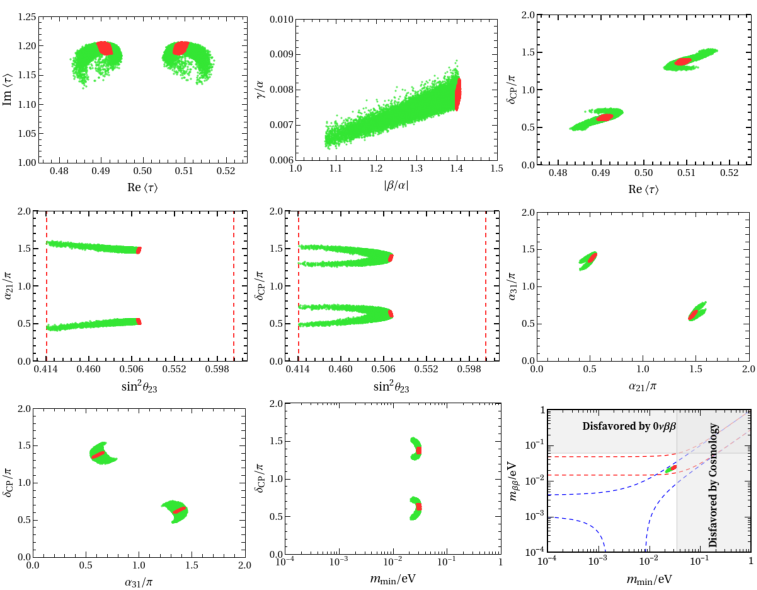
Refer to caption
Figure 1: The predicted correlations among the input free parameters, neutrino mixing angles and CP violating phases in the lepton model ℒ22\mathcal{L}_{22} with (red) and without (green) gCP symmetry.

5 Unified description of all fermions

As shown in previous section, one can construct predictive lepton models based on the homogeneous finite modular group A5′A^{\prime}_{5}. In this section, we shall apply A5′A^{\prime}_{5} to explain the quark masses and CKM mixing matrix. Analogous to what we have done for charged lepton sector in section 4.1, we can systematically analyze the possible quark models with A5′A^{\prime}_{5} modular symmetry. We find that the measured quark masses and CKM mixing matrix can be explained in terms of a few free parameters if quark fields are embedded in doublet and singlet representations of A5′A^{\prime}_{5}. We have made a systematic classification of quark models for this kind of quark arrangement and generalize the strategy of numerical analysis for leptons to the quark sector. The values of quark masses and CKM parameters are taken from [74],

mu/mc=(1.9286±0.6017)×10−3,mc/mt=(2.8213±0.1195)×10−3,\displaystyle m_{u}/m_{c}=(1.9286\pm 0.6017)\times 10^{-3}\,,\quad m_{c}/m_{t}=(2.8213\pm 0.1195)\times 10^{-3}\,,
md/ms=(5.0523±0.6191)×10−2,ms/mb=(1.8241±0.1005)×10−2,\displaystyle m_{d}/m_{s}=(5.0523\pm 0.6191)\times 10^{-2}\,,\quad m_{s}/m_{b}=(1.8241\pm 0.1005)\times 10^{-2}\,,
mt=87.4555​GeV,mb=0.9682​GeV,δC​Pq/π=0.3845±0.0173,\displaystyle m_{t}=87.4555\mathrm{GeV}\,,\quad m_{b}=0.9682\mathrm{GeV}\,,\quad\delta_{CP}^{q}/\pi=0.3845\pm 0.0173\,,
θ12q=0.22736±0.00073,θ13q=0.00349±0.00013,θ23q=0.04015±0.00064,\displaystyle\theta_{12}^{q}=0.22736\pm 0.00073\,,\quad\theta_{13}^{q}=0.00349\pm 0.00013\,,\quad\theta_{23}^{q}=0.04015\pm 0.00064\,, (70)

which are calculated at the GUT scale with tan⁡β=10\tan\beta=10 and the SUSY breaking scale MSUSY=10M_{\text{SUSY}}=10 TeV. In the end, we find four models out of 892 possibilities can describe the experimental data of quarks with 11 free parameters including Re​(τ)\texttt{Re}(\tau) and Im​(τ)\texttt{Im}(\tau). A systematic classification of the quark models as well as the numerical results are included in the supplementary file [72].

Furthermore, we combine the 2525 viable lepton models collected in table 4 with the two candidate quark models to give a unified description of quark and lepton in a single model. The crucial point is whether there exist common values of τ\tau for which the experimental data of both quarks and leptons can be reproduced. It is remarkable that we really find a quark-lepton unification model: the lepton sector is the model ℒ2\mathcal{L}_{2} and the quark sector is 𝒬3\mathcal{Q}_{3} which can be found in the supplementary material [72]. In the model 𝒬3\mathcal{Q}_{3}, the quark fields and the Higgs fields transform under modular symmetry as follows,

ρQ=𝟐′⊕𝟏,ρUc=ρDc=𝟐′⊕𝟏,ρHu=ρHd=𝟏,\displaystyle\rho_{Q}=\mathbf{2^{\prime}}\oplus\mathbf{1}\,,\quad\rho_{U^{c}}=\rho_{D^{c}}=\mathbf{2^{\prime}}\oplus\mathbf{1}\,,\quad\rho_{H_{u}}=\rho_{H_{d}}=\mathbf{1}\,,
kQ3=kQD−5=−kUDc−3=−kU3c=−kDDc−1=−kD3c,kHu=kHd=0,\displaystyle k_{Q_{3}}=k_{Q_{D}}-5=-k_{U^{c}_{D}}-3=-k_{U^{c}_{3}}=-k_{D^{c}_{D}}-1=-k_{D^{c}_{3}}\,,\quad k_{H_{u}}=k_{H_{d}}=0\,, (71)

where we denote QD≡(Q1,Q2)T,UDc≡(U1c,U2c)T,DDc≡(D1c,D2c)TQ_{D}\equiv(Q_{1},~Q_{2})^{T},\,U^{c}_{D}\equiv(U_{1}^{c},~U_{2}^{c})^{T},\,D^{c}_{D}\equiv(D^{c}_{1},~D^{c}_{2})^{T}, and the modular weight kQk_{Q} is a general integer. Thus the modular invariant superpotentials of quark sector are given by

𝒲u=αu​(Y𝟑′(2)​UDc​QD​Hu)𝟏+βu​(Y𝟐′(5)​U3c​QD​Hu)𝟏+γu​(U3c​Q3​Hu)𝟏,\displaystyle\mathcal{W}_{u}=\alpha_{u}\left(Y_{\mathbf{3}^{\prime}}^{(2)}U^{c}_{D}Q_{D}H_{u}\right)_{\mathbf{1}}+\beta_{u}\left(Y_{\mathbf{2}^{\prime}}^{(5)}U^{c}_{3}Q_{D}H_{u}\right)_{\mathbf{1}}+\gamma_{u}\left(U^{c}_{3}Q_{3}H_{u}\right)_{\mathbf{1}}\,,
𝒲d=αd​(Y𝟏(4)​DDc​QD​Hd)𝟏+βd​(Y𝟑′(4)​DDc​QD​Hd)𝟏+γd​(Y𝟐′(5)​D3c​QD​Hd)𝟏+δd​(D3c​Q3​Hd)𝟏.\displaystyle\mathcal{W}_{d}=\alpha_{d}\left(Y_{\mathbf{1}}^{(4)}D^{c}_{D}Q_{D}H_{d}\right)_{\mathbf{1}}+\beta_{d}\left(Y_{\mathbf{3}^{\prime}}^{(4)}D^{c}_{D}Q_{D}H_{d}\right)_{\mathbf{1}}+\gamma_{d}\left(Y_{\mathbf{2}^{\prime}}^{(5)}D^{c}_{3}Q_{D}H_{d}\right)_{\mathbf{1}}+\delta_{d}\left(D^{c}_{3}Q_{3}H_{d}\right)_{\mathbf{1}}\,. (72)

The phases of αu\alpha_{u}, βu\beta_{u}, γu\gamma_{u}, αd\alpha_{d} and γd\gamma_{d} are unphysical and they can be absorbed by quark fields, nevertheless the phases of βd\beta_{d} and δd\delta_{d} can not be removed by field redefinition. The corresponding up and down quark masses matrices can be written as

Mu=(−2​αu​Y𝟑′,3(2)αu​Y𝟑′,1(2)0αu​Y𝟑′,1(2)2​αu​Y𝟑′,2(2)0−βu​Y𝟐′,2(5)βu​Y𝟐′,1(5)γu)​vu,Md=(−2​βd​Y𝟑′,3(4)βd​Y𝟑′,1(4)−αd​Y𝟏,1(4)0αd​Y𝟏,1(4)+βd​Y𝟑′,1(4)2​βd​Y𝟑′,2(4)0−γd​Y𝟐′,2(5)γd​Y𝟐′,1(5)δd)​vd.\displaystyle M_{u}=\begin{pmatrix}-\sqrt{2}\alpha_{u}Y_{\mathbf{3}^{\prime},3}^{(2)}&\alpha_{u}Y_{\mathbf{3}^{\prime},1}^{(2)}&0\\ \alpha_{u}Y_{\mathbf{3}^{\prime},1}^{(2)}&\sqrt{2}\alpha_{u}Y_{\mathbf{3}^{\prime},2}^{(2)}&0\\ -\beta_{u}Y_{\mathbf{2}^{\prime},2}^{(5)}&\beta_{u}Y_{\mathbf{2}^{\prime},1}^{(5)}&\gamma_{u}\\ \end{pmatrix}v_{u}\,,~M_{d}=\begin{pmatrix}-\sqrt{2}\beta_{d}Y_{\mathbf{3}^{\prime},3}^{(4)}&\beta_{d}Y_{\mathbf{3}^{\prime},1}^{(4)}-\alpha_{d}Y_{\mathbf{1},1}^{(4)}&0\\ \alpha_{d}Y_{\mathbf{1},1}^{(4)}+\beta_{d}Y_{\mathbf{3}^{\prime},1}^{(4)}&\sqrt{2}\beta_{d}Y_{\mathbf{3}^{\prime},2}^{(4)}&0\\ -\gamma_{d}Y_{\mathbf{2}^{\prime},2}^{(5)}&\gamma_{d}Y_{\mathbf{2}^{\prime},1}^{(5)}&\delta_{d}\\ \end{pmatrix}v_{d}\,. (73)

Notice that both (13) and (23) entries of MuM_{u} and MdM_{d} vanish exactly. This model uses 15 real dimensionless parameters to describe the mixing angles, CP violation phases and the masses ratios of both quarks and leptons. The 4 overall scale factors α​vd\alpha v_{d}, g1​vu2/Λg_{1}v_{u}^{2}/\Lambda, αu​vu\alpha_{u}v_{u} and αd​vd\alpha_{d}v_{d} give the absolute masses scale of the charged leptons, neutrinos, up quarks and down quarks. By scanning the parameter space of the complete model, we identify the best fit point of the input parameters,

⟨τ⟩=−0.499996+0.894402​i,β/α=24.5400,γ/α=654.9320,δ/α=100.8429​e4.3652​i,\displaystyle\langle\tau\rangle=-0.499996+0.894402i\,,~~\beta/\alpha=24.5400\,,~~\gamma/\alpha=654.9320\,,~~\delta/\alpha=100.8429e^{4.3652i}\,,
g2/g1=0.3818​e5.5110​i,βu/αu=32.6296,γu/αu=11.1981,βd/αd=6.3229​e0.00068​i,\displaystyle g_{2}/g_{1}=0.3818e^{5.5110i}\,,~~\beta_{u}/\alpha_{u}=32.6296\,,~~\gamma_{u}/\alpha_{u}=11.1981\,,~~\beta_{d}/\alpha_{d}=6.3229e^{0.00068i}\,,
γd/αd=1.7462,δd/αd=1.9895​e5.4463​i,α​vd=0.04361​MeV,g1​vu2/Λ=1.0895​meV,\displaystyle\gamma_{d}/\alpha_{d}=1.7462\,,~~\delta_{d}/\alpha_{d}=1.9895e^{5.4463i}\,,~~\alpha v_{d}=0.04361~\text{MeV}\,,~~g_{1}v_{u}^{2}/\Lambda=1.0895~\text{meV}\,,
αu​vu=0.03432​GeV,αd​vd=0.00243​GeV.\displaystyle\alpha_{u}v_{u}=0.03432~\text{GeV}\,,\quad\alpha_{d}v_{d}=0.00243~\text{GeV}\,. (74)

The corresponding predictions for masses and mixing parameters of quarks and leptons are determined to be

sin2⁡θ13l=0.02231,sin2⁡θ12l=0.3019,sin2⁡θ23l=0.4570,δC​Pl=1.1671​π,\displaystyle\sin^{2}\theta^{l}_{13}=0.02231\,,\quad\sin^{2}\theta^{l}_{12}=0.3019\,,\quad\sin^{2}\theta^{l}_{23}=0.4570\,,\quad\delta^{l}_{CP}=1.1671\pi\,,
α21=1.3593​π,α31=0.4762​π,me/mμ=0.00474,mμ/mτ=0.05857,\displaystyle\alpha_{21}=1.3593\pi\,,\quad\alpha_{31}=0.4762\pi\,,\quad m_{e}/m_{\mu}=0.00474\,,\quad m_{\mu}/m_{\tau}=0.05857\,,
m1=77.2709​meV,m2=77.7495​meV,m3=92.1717​meV,\displaystyle m_{1}=77.2709~\text{meV}\,,\quad m_{2}=77.7495~\text{meV}\,,\quad m_{3}=92.1717~\text{meV}\,,
∑imi=247.1921​meV,mβ=77.7755​meV,mβ​β=48.9783​meV,\displaystyle\sum_{i}m_{i}=247.1921~\text{meV}\,,\quad m_{\beta}=77.7755~\text{meV}\,,\quad m_{\beta\beta}=48.9783~\text{meV}\,,
θ13q=0.003498,θ12q=0.22764,θ23q=0.04023,δC​Pq=69.1740∘,\displaystyle\theta^{q}_{13}=0.003498\,,\quad\theta^{q}_{12}=0.22764\,,\quad\theta^{q}_{23}=0.04023\,,\quad\delta^{q}_{CP}=69.1740^{\circ}\,,
mu/mc=0.00021,mc/mt=0.00282,md/ms=0.03457,ms/mb=0.01769,\displaystyle m_{u}/m_{c}=0.00021\,,\quad m_{c}/m_{t}=0.00282\,,\quad m_{d}/m_{s}=0.03457\,,\quad m_{s}/m_{b}=0.01769\,, (75)

which are in the experimentally preferred 3​σ3\sigma ranges. It is interesting to note that the common value of τ\tau is very close to the fixed point τS​T=e2​π​i/3\tau_{ST}=e^{2\pi i/3} which preserves a Z3S​TZ^{ST}_{3} residual symmetry.

6 Extension to rational weight modular forms at level 5

The modular weights could be rational numbers, as shown in the string construction [79, 80, 11]. It is interesting to study the fractional weight modular forms from the bottom-up modular invariance approach. To discuss rational weight modular forms, it is convenient to consider the metaplectic cover of the modular group S​L​(2,ℤ)SL(2,\mathbb{Z}) [58]. For the concerned case, we should consider the 5-fold covering of S​L​(2,ℤ)SL(2,\mathbb{Z}) and it is denoted as Γ~\widetilde{\Gamma} with

Γ~={γ~=(γ,ϕ(γ,τ))|γ∈(abcd)∈SL(2,ℤ),ϕ(γ,τ)5=(cτ+d)}.\widetilde{\Gamma}=\Big\{\widetilde{\gamma}=(\gamma,\phi(\gamma,\tau))~|~\gamma\in\begin{pmatrix}a&b\\ c&d\end{pmatrix}\in SL(2,\mathbb{Z}),\quad\phi(\gamma,\tau)^{5}=(c\tau+d)\Big\}\,. (76)

The action of γ~\widetilde{\gamma} on τ\tau is the same as that of γ\gamma, i.e. γ~​τ=γ​τ\widetilde{\gamma}\tau=\gamma\tau. The group multiplication of Γ~\widetilde{\Gamma} is defined as

(γ1,ϕ1​(γ1,τ))​(γ2,ϕ2​(γ2,τ))=(γ1​γ2,ϕ1​(γ1,γ2​τ)​ϕ2​(γ2,τ)),(\gamma_{1},\phi_{1}(\gamma_{1},\tau))(\gamma_{2},\phi_{2}(\gamma_{2},\tau))=(\gamma_{1}\gamma_{2},\phi_{1}(\gamma_{1},\gamma_{2}\tau)\phi_{2}(\gamma_{2},\tau))\,, (77)

where ϕ1=ϵ1​(c​τ+d)1/5\phi_{1}=\epsilon_{1}(c\tau+d)^{1/5}, ϕ2=ϵ2​(c​τ+d)1/5\phi_{2}=\epsilon_{2}(c\tau+d)^{1/5} and ϵ1,2∈{1,ω5,ω52,ω53,ω54}\epsilon_{1,2}\in\{1,\omega_{5},\omega_{5}^{2},\omega_{5}^{3},\omega_{5}^{4}\}. The principal branch of the quintic root is chosen here. Obviously each element γ∈S​L​(2,ℤ)\gamma\in SL(2,\mathbb{Z}) corresponds to five element γ~=(γ,ω5j​(c​τ+d)1/5)\tilde{\gamma}=(\gamma,\omega^{j}_{5}(c\tau+d)^{1/5}) of the metaplectic group Γ~\widetilde{\Gamma} with ω5=e2​π​i/5\omega_{5}=e^{2\pi i/5} and j=0,1,2,3,4j=0,1,2,3,4. The group Γ~\widetilde{\Gamma} can be generated by

S~=((01−10),ω52​(−τ)1/5),T~=((1101),1),\widetilde{S}=\left(\begin{pmatrix}0&1\\ -1&0\end{pmatrix}\,,~\omega_{5}^{2}(-\tau)^{1/5}\right)\,,\quad\widetilde{T}=\left(\begin{pmatrix}1&1\\ 0&1\end{pmatrix}\,,1\right)\,, (78)

where (−τ)1/5(-\tau)^{1/5} denotes the principal branch of quintic root, possessing positive real part. It follows that

S~2=R~,R~10=1,(S~​T~)3=1,\widetilde{S}^{2}=\widetilde{R}\,,\quad\widetilde{R}^{10}=1\,,\quad(\widetilde{S}\widetilde{T})^{3}=1\,, (79)

with

R~=((−100−1),−ω5).\widetilde{R}=\left(\begin{pmatrix}-1&0\\ 0&-1\end{pmatrix}\,,-\omega_{5}\right)\,. (80)

Therefore the elements S~\widetilde{S} and S~​T~\widetilde{S}\widetilde{T} are of orders 20 and 3 respectively while T~\widetilde{T} is of infinite order. Obviously the element R~\widetilde{R} generates the center of Γ~5\widetilde{\Gamma}_{5}. The metaplectic principal congruence subgroup at level 5 is defined as

Γ~​(5)={h~=(h,v5​(h)​J1/5​(h,τ))|h∈Γ⁡(5)},\widetilde{\Gamma}(5)=\Big\{\widetilde{h}=(h,v_{5}(h)J_{1/5}(h,\tau))\Big|h\in\Gamma(5)\Big\}\,, (81)

where J1/5​(h,τ)=(c​τ+d)1/5J_{1/5}(h,\tau)=(c\tau+d)^{1/5}, v5​(h)v_{5}(h) is the multiplier of the weight 1/51/5 modular forms33 3 The weight 1/51/5 modular forms for Γ⁡(5)\Gamma(5) are holomorphic functions satisfying f⁡(γ​τ)=v5​(γ)​(c​τ+d)1/5​f​(τ)f(\gamma\tau)=v_{5}(\gamma)(c\tau+d)^{1/5}f(\tau) for γ∈Γ⁡(5)\gamma\in\Gamma(5). for Γ⁡(5)\Gamma(5), and the identity v55​(h)=1v^{5}_{5}(h)=1 is fulfilled for all h∈Γ⁡(5)h\in\Gamma(5). The explicit expression of v5​(h)v_{5}(h) has been given in [68, 58], it is too lengthy to present here. It is obvious that Γ~​(5)\widetilde{\Gamma}(5) is isomorphic to Γ⁡(5)\Gamma(5), and it is a normal subgroup of Γ~\widetilde{\Gamma}. In particular, the element T~5\widetilde{T}^{5} belongs to Γ~​(5)\widetilde{\Gamma}(5). Taking the group quotient, we can obtain the finite metaplectic group Γ~5=\widetilde{\Gamma}_{5}= Γ~/Γ⁡(5)≅A5′×Z5\widetilde{\Gamma}/\Gamma(5)\cong A^{\prime}_{5}\times Z_{5} which can be obtained by imposing another condition T~5=1\widetilde{T}^{5}=1. Thus the generator relations of Γ~5\widetilde{\Gamma}_{5} are

S~2=R~,R~10=1,(S~​T~)3=T~5=1,R~​T~=T~​R~.\widetilde{S}^{2}=\widetilde{R}\,,\quad\widetilde{R}^{10}=1\,,\quad(\widetilde{S}\widetilde{T})^{3}=\widetilde{T}^{5}=1\,,\quad\widetilde{R}\widetilde{T}=\widetilde{T}\widetilde{R}\,. (82)

The group ID of Γ~5\widetilde{\Gamma}_{5} in GAP system is [600,54][600,54], and it is isomorphic to the direct product of A5′A^{\prime}_{5} and Z5Z_{5}, i.e., Γ~5≅A5′×Z5\widetilde{\Gamma}_{5}\cong A^{\prime}_{5}\times Z_{5}. Hence it is more convenient to choose another set of generators SS, TT and UU which obey the relations

S2=R,(S​T)3=T5=R2=1,U5=1,U​S=S​U,U​T=T​U.S^{2}=R,\quad(ST)^{3}=T^{5}=R^{2}=1,\quad U^{5}=1,\quad US=SU,\quad UT=TU\,. (83)

Notice that the generators SS and TT generate a A5′A^{\prime}_{5} subgroup, and UU generates a Z5Z_{5} subgroup. The generators SS, TT and UU are related to S~\widetilde{S}, T~\widetilde{T} as follows

S=R~2​S~=((01−10),ω54​(−τ)1/5),\displaystyle S=\widetilde{R}^{2}\widetilde{S}=\left(\begin{pmatrix}0&1\\ -1&0\end{pmatrix}\,,~\omega_{5}^{4}(-\tau)^{1/5}\right)\,,
T=R~−2​T~=((1101),ω53),\displaystyle T=\widetilde{R}^{-2}\widetilde{T}=\left(\begin{pmatrix}1&1\\ 0&1\end{pmatrix}\,,\omega^{3}_{5}\right)\,,
U=S~12=((1001),ω5),\displaystyle U=\widetilde{S}^{12}=\left(\begin{pmatrix}1&0\\ 0&1\end{pmatrix}\,,\omega_{5}\right)\,, (84)

and vice versa

S~=U−2​S,T~=U2​T,R~=U​R.\widetilde{S}=U^{-2}S,\quad\widetilde{T}=U^{2}T,\quad\widetilde{R}=UR\,. (85)

The irreducible representations of Γ~5\widetilde{\Gamma}_{5} can be obtained from the tensor products of the irreducible representations of A5′A^{\prime}_{5} and Z5UZ^{U}_{5} where the superscript UU denotes the generator of the Z5Z_{5} subgroup. The irreducible representations of A5′A^{\prime}_{5} are summarized in table 11, and abelian subgroup Z5UZ^{U}_{5} has five one-dimensional irreducible representations and the generator UU is represented by ω5j\omega^{j}_{5} with j=0,1,2,3,4j=0,1,2,3,4. We shall denote the irreducible representation of Γ~5\widetilde{\Gamma}_{5} as 𝐫j\mathbf{r}^{j} which is the tensor product of the A5′A^{\prime}_{5} irreducible representation 𝐫\mathbf{r} with the Z5UZ^{U}_{5} representation ω5j\omega^{j}_{5}. The generators SS, TT and UU are represented by

𝐫j:ρ𝐫j​(S)=ρ𝐫​(S),ρ𝐫j​(T)=ρ𝐫​(T),ρ𝐫j​(U)=ω5j,\displaystyle\mathbf{r}^{j}~:~\rho_{\mathbf{r}^{j}}(S)=\rho_{\mathbf{r}}(S)\,,\quad\rho_{\mathbf{r}^{j}}(T)=\rho_{\mathbf{r}}(T)\,,\quad\rho_{\mathbf{r}^{j}}(U)=\omega_{5}^{j}\,, (86)

where ρ𝐫\rho_{\mathbf{r}} is the representation matrix of the A5′A^{\prime}_{5} irreducible representation 𝐫\mathbf{r} as shown in Appendix A. The Kronecker products of Γ~5\widetilde{\Gamma}_{5} can be easily obtained from those of A5′A^{\prime}_{5} given in Eq. (A.12) by including an extra index jj for each A5′A^{\prime}_{5} representation. For instance, we have 𝟐3⊗𝟑4=𝟐2⊕𝟒′2\mathbf{2}^{3}\otimes\mathbf{3}^{4}=\mathbf{2}^{2}\oplus\mathbf{4}^{\prime 2}, and the corresponding Clebsch-Gordan coefficients coefficients remains the same as those of A5′A^{\prime}_{5}, which are listed in the Appendix A.

It has been shown that the modular forms of weight k/5k/5 (k:k: non-negative integers) can be constructed for the principal congruence subgroup Γ⁡(5)\Gamma(5) [68], and a multiplier v5​(γ)v_{5}(\gamma) is necessary so that v⁡(γ)​(c​τ+d)k/5v(\gamma)(c\tau+d)^{k/5} is the correct automorphy factor satisfying the cocycle relation. The graded ring of modular forms of weight k/5k/5 at level 5 can be generated by two algebraically independent weight 1/51/5 modular forms  [68]:

ℳ⁡(Γ⁡(5))=ℂ⁡[f1​(τ),f2​(τ)],\mathcal{M}(\Gamma(5))=\mathbb{C}[f_{1}(\tau),~f_{2}(\tau)]\,, (87)

with

f1​(τ)=θ(110,12)​(5​τ)η​(τ)3/5,f2​(τ)=θ(310,12)​(5​τ)η​(τ)3/5.f_{1}(\tau)=\dfrac{\theta_{(\frac{1}{10},\frac{1}{2})}(5\tau)}{\eta(\tau)^{3/5}}\,,~~~~f_{2}(\tau)=\dfrac{\theta_{(\frac{3}{10},\frac{1}{2})}(5\tau)}{\eta(\tau)^{3/5}}\,. (88)

Notice that the theta constant is defined as [68]

θ(m′,m′′)​(τ)=∑m∈ℤe2​π​i​[12​(m+m′)2​τ+(m+m′)​m′′],\theta_{(m^{\prime},m^{\prime\prime})}(\tau)=\sum_{m\in\mathbb{Z}}e^{2\pi i[\frac{1}{2}(m+m^{\prime})^{2}\tau+(m+m^{\prime})m^{\prime\prime}]}\,, (89)

and η⁡(τ)\eta(\tau) is the well-known Dedekind eta function given in Eq. (B.2). Hence the linear space of the modular forms of weight k/5k/5 and level 5 has dimension k+1k+1, and the linear independent basis vectors are k+1k+1 polynomials of f1f_{1} and f2f_{2} with degree kk. Under the action of the generators SS and TT of the modular group, f1f_{1} and f2f_{2} transform as [68]

f1​(τ)→𝑆f1​(−1τ)=ω52​(−τ)1/5​15​[(ω53−ω5)​f1​(τ)+(ω52−ω5)​f2​(τ)],,\displaystyle f_{1}(\tau)\xrightarrow{S}f_{1}(-\frac{1}{\tau})=\omega_{5}^{2}(-\tau)^{1/5}\frac{1}{\sqrt{5}}\left[\left(\omega_{5}^{3}-\omega_{5}\right)f_{1}(\tau)+\left(\omega_{5}^{2}-\omega_{5}\right)f_{2}(\tau)\right],\,,
f2​(τ)→𝑆f2​(−1τ)=ω52​(−τ)1/5​15​[(ω53−ω52)​f1​(τ)+(ω5−ω53)​f2​(τ)],\displaystyle f_{2}(\tau)\xrightarrow{S}f_{2}(-\frac{1}{\tau})=\omega_{5}^{2}(-\tau)^{1/5}\frac{1}{\sqrt{5}}\left[\left(\omega_{5}^{3}-\omega_{5}^{2}\right)f_{1}(\tau)+\left(\omega_{5}-\omega_{5}^{3}\right)f_{2}(\tau)\right]\,,
f1​(τ)→𝑇f1​(τ+1)=f1​(τ),f2​(τ)→𝑇f2​(τ+1)=ω5​f2​(τ).\displaystyle f_{1}(\tau)\xrightarrow{T}f_{1}(\tau+1)=f_{1}(\tau),~~~~f_{2}(\tau)\xrightarrow{T}f_{2}(\tau+1)=\omega_{5}f_{2}(\tau)\,. (90)

Analogous to the half-integral weight modular forms [58], the modular forms of weight r=k/5r=k/5 and level 5 can be arranged into different irreducible representations Y𝐫j(r)​(τ)Y^{(r)}_{\mathbf{r}^{j}}(\tau) of the finite metaplectic group Γ~5\widetilde{\Gamma}_{5}. The modular multiplet Y𝐫j(r)​(τ)Y^{(r)}_{\mathbf{r}^{j}}(\tau) transform under Γ~5=Γ~/Γ~​(5)\widetilde{\Gamma}_{5}=\widetilde{\Gamma}/\widetilde{\Gamma}(5) as

Y𝐫j(r)​(γ~​τ)=ϕ5​r​(γ,τ)​ρ𝐫j​(γ~)​Y𝐫j(r)​(τ),Y^{(r)}_{\mathbf{r}^{j}}(\widetilde{\gamma}\tau)=\phi^{5r}(\gamma,\tau)\rho_{\mathbf{r}^{j}}(\widetilde{\gamma})Y^{(r)}_{\mathbf{r}^{j}}(\tau)\,, (91)

where γ~\widetilde{\gamma} stands for a representative element of Γ~5\widetilde{\Gamma}_{5}. Applying Eq. (91) to the element γ~=U\widetilde{\gamma}=U, we find that the constraint 5​r+j=0​(mod​5)5r+j=0\,(\texttt{mod}~5) should be fulfilled. In the group representation basis chosen above, the two weight 1/51/5 modular forms can be arranged into a Γ~5\widetilde{\Gamma}_{5} doublet 𝟐4\mathbf{2}^{4} as follows,

Y𝟐4(15)​(τ)≡(F1​(τ)F2​(τ)),F1​(τ)=e−π​i10​f1​(τ),F2​(τ)=e−3​π​i10​f2​(τ).Y^{(\frac{1}{5})}_{\mathbf{2}^{4}}(\tau)\equiv\begin{pmatrix}F_{1}(\tau)\\ F_{2}(\tau)\end{pmatrix},~~~F_{1}(\tau)=e^{-\frac{\pi i}{10}}f_{1}(\tau),~~~F_{2}(\tau)=e^{-\frac{3\pi i}{10}}f_{2}(\tau)\,. (92)

The qq-series expressions of F1​(τ)F_{1}(\tau) and F2​(τ)F_{2}(\tau) are given by

F1​(τ)​η​(τ)3/5=q1/40​∑m∈ℤ(−1)m​q(5​m2+m)/2,F2​(τ)​η​(τ)3/5=q9/40​∑m∈ℤ(−1)m​q(5​m2+3​m)/2,F_{1}(\tau)\,\eta(\tau)^{3/5}=q^{1/40}\sum_{m\in\mathbb{Z}}(-1)^{m}q^{(5m^{2}+m)/2},~~~~F_{2}(\tau)\,\eta(\tau)^{3/5}=q^{9/40}\sum_{m\in\mathbb{Z}}(-1)^{m}q^{(5m^{2}+3m)/2}\,, (93)

with q=e2​π​i​τq=e^{2\pi i\tau}. Using the transformation rules in Eq. (90), we find that Y𝟐4(15)​(τ)Y^{(\frac{1}{5})}_{\mathbf{2}^{4}}(\tau) really transforms in the two-dimensional representation 𝟐4\mathbf{2}^{4} of Γ~5\widetilde{\Gamma}_{5},

Y𝟐4(15)​(τ)→𝑆Y𝟐4(15)​(−1τ)=ω54​(−τ)1/5​ρ𝟐4​(S)​Y𝟐4(15)​(τ),\displaystyle Y^{(\frac{1}{5})}_{\mathbf{2}^{4}}(\tau)\xrightarrow{S}Y^{(\frac{1}{5})}_{\mathbf{2}^{4}}(-\frac{1}{\tau})=\omega_{5}^{4}(-\tau)^{1/5}\,\rho_{\mathbf{2}^{4}}(S)Y^{(\frac{1}{5})}_{\mathbf{2}^{4}}(\tau)\,,
Y𝟐4(15)​(τ)→𝑇Y𝟐4(15)​(τ+1)=ω53​ρ𝟐4​(T)​Y𝟐4(15)​(τ),\displaystyle Y^{(\frac{1}{5})}_{\mathbf{2}^{4}}(\tau)\xrightarrow{T}Y^{(\frac{1}{5})}_{\mathbf{2}^{4}}(\tau+1)=\omega^{3}_{5}\,\rho_{\mathbf{2}^{4}}(T)Y^{(\frac{1}{5})}_{\mathbf{2}^{4}}(\tau)\,, (94)

and it is invariant under the generator UU. Using the Clebsch-Gordan coefficients of Γ~5\widetilde{\Gamma}_{5}, we can construct the higher rational weight modular forms through the tensor products of Y𝟐4(15)​(τ)Y^{(\frac{1}{5})}_{\mathbf{2}^{4}}(\tau). At weight r=2/5r=2/5, we have

Y𝟑3(25)=−12​(Y𝟐4(15)​Y𝟐4(15))𝟑3=(2​F1​F2−F22F12),\displaystyle Y^{(\frac{2}{5})}_{\mathbf{3}^{3}}=-\frac{1}{\sqrt{2}}\left(Y^{(\frac{1}{5})}_{\mathbf{2}^{4}}Y^{(\frac{1}{5})}_{\mathbf{2}^{4}}\right)_{\mathbf{3}^{3}}=\begin{pmatrix}\sqrt{2}F_{1}F_{2}\\ -F_{2}^{2}\\ F_{1}^{2}\end{pmatrix}\,, (95)

where an overall constant −12-\frac{1}{\sqrt{2}} is multiplied to make the resulting expression relatively simple. Note that another contraction (Y𝟐4(15)​Y𝟐4(15))𝟏3=0\left(Y^{(\frac{1}{5})}_{\mathbf{2}^{4}}Y^{(\frac{1}{5})}_{\mathbf{2}^{4}}\right)_{\mathbf{1}^{3}}=0 because of the antisymmetric Clebsch-Gordan coefficients. In exactly the same fashion, other rational weight modular forms can be obtained, and we present linearly independent rational weight modular forms up to weight 11:

r=3/5:Y𝟒′2(35)=−13​(Y𝟐4(15)​Y𝟑3(25))𝟒′2=(F13−3​F12​F23​F1​F22F23),\displaystyle r=3/5:~~~~~~~~~Y^{(\frac{3}{5})}_{\mathbf{4}^{\prime 2}}=-\frac{1}{\sqrt{3}}\left(Y^{(\frac{1}{5})}_{\mathbf{2}^{4}}Y^{(\frac{2}{5})}_{\mathbf{3}^{3}}\right)_{\mathbf{4}^{\prime 2}}=\begin{pmatrix}F_{1}^{3}\\ -\sqrt{3}F_{1}^{2}F_{2}\\ \sqrt{3}F_{1}F_{2}^{2}\\ F_{2}^{3}\\ \end{pmatrix}, (96)
r=4/5:Y𝟓1(45)=12​(Y𝟐4(15)​Y𝟒′2(35))𝟓1=(6​F12​F222​F1​F23F24F14−2​F13​F2),\displaystyle r=4/5:~~~~~~~~~Y^{(\frac{4}{5})}_{\mathbf{5}^{1}}=\frac{1}{2}\left(Y^{(\frac{1}{5})}_{\mathbf{2}^{4}}Y^{(\frac{3}{5})}_{\mathbf{4}^{\prime 2}}\right)_{\mathbf{5}^{1}}=\begin{pmatrix}\sqrt{6}F_{1}^{2}F_{2}^{2}\\ 2F_{1}F_{2}^{3}\\ F_{2}^{4}\\ F_{1}^{4}\\ -2F_{1}^{3}F_{2}\end{pmatrix}, (97)
r=1:Y𝟔0(1)=−(Y𝟐4(15)​Y𝟓1(45))𝟔0=(F15+2​F252​F15−F255​F14​F25​2​F13​F22−5​2​F12​F235​F1​F24).\displaystyle r=1:~~~~~~~~~Y^{(1)}_{\mathbf{6}^{0}}=-\left(Y^{(\frac{1}{5})}_{\mathbf{2}^{4}}Y^{(\frac{4}{5})}_{\mathbf{5}^{1}}\right)_{\mathbf{6}^{0}}=\begin{pmatrix}F_{1}^{5}+2F_{2}^{5}\\ 2F_{1}^{5}-F_{2}^{5}\\ 5F_{1}^{4}F_{2}\\ 5\sqrt{2}F_{1}^{3}F_{2}^{2}\\ -5\sqrt{2}F_{1}^{2}F_{2}^{3}\\ 5F_{1}F_{2}^{4}\end{pmatrix}\,. (98)

From Eqs. (93, B.2), we can read out the qq-expansion of the Y𝟔0(1)Y^{(1)}_{\mathbf{6}^{0}} as follow,

Y𝟔0(1)​(τ)=(1+5​q+10​q3−5​q4+5​q5+…2+5​q+10​q2+5​q4+5​q5+…5​q1/5​(1+2​q+2​q2+q3+2​q4+2​q5+…)5​2​q2/5​(1+q+q2+q3+2​q4+q6+…)−5​2​q3/5​(1+q2+q3+q4−q5+…)5​q4/5​(1−q+2​q2+2​q6−2​q7+…)),Y^{(1)}_{\mathbf{6}^{0}}(\tau)=\begin{pmatrix}1+5q+10q^{3}-5q^{4}+5q^{5}+\dots\\ 2+5q+10q^{2}+5q^{4}+5q^{5}+\dots\\ 5q^{1/5}\left(1+2q+2q^{2}+q^{3}+2q^{4}+2q^{5}+\dots\right)\\ 5\sqrt{2}q^{2/5}\left(1+q+q^{2}+q^{3}+2q^{4}+q^{6}+\dots\right)\\ -5\sqrt{2}q^{3/5}\left(1+q^{2}+q^{3}+q^{4}-q^{5}+\dots\right)\\ 5q^{4/5}\left(1-q+2q^{2}+2q^{6}-2q^{7}+\dots\right)\end{pmatrix}\,, (99)

which is exactly identical with the q−q-expansion expressions of weight 1 modular form obtained from the Dedekind eta function and Klein forms in Eq. (B.10). Furthermore, comparing Eq. (98) with Eq. (B.8), we find that theta constants and the Klein forms are closely related as follows

θ(110,12)​(τ)=eπ​i10​η3​(τ)​𝔨25,0​(τ),θ(310,12)​(τ)=e3​π​i10​η3​(τ)​𝔨15,0​(τ).\theta_{(\frac{1}{10},\frac{1}{2})}(\tau)=e^{\frac{\pi i}{10}}\eta^{3}(\tau)\mathfrak{k}_{\frac{2}{5},0}(\tau)\,,~~~\theta_{(\frac{3}{10},\frac{1}{2})}(\tau)=e^{\frac{3\pi i}{10}}\eta^{3}(\tau)\mathfrak{k}_{\frac{1}{5},0}(\tau)\,. (100)

These two identities can be proved by using the famous Jacobi triple product identity as shown in Appendix C. As a consequence, the basis vectors e1,2,3,4,5,6​(τ)e_{1,2,3,4,5,6}(\tau) of weight 1 modular form at level 5 are polynomials of degree 5 in F1​(τ)F_{1}(\tau) and F2​(τ)F_{2}(\tau),

e1​(τ)=F15​(τ),e2​(τ)=F14​(τ)​F2​(τ),e3​(τ)=F13​(τ)​F22​(τ),\displaystyle e_{1}(\tau)=F_{1}^{5}(\tau)\,,~~~~e_{2}(\tau)=F_{1}^{4}(\tau)F_{2}(\tau)\,,~~~~e_{3}(\tau)=F_{1}^{3}(\tau)F_{2}^{2}(\tau)\,,~~
e4​(τ)=F12​(τ)​F23​(τ),e5​(τ)=F1​(τ)​F24​(τ),e6​(τ)=F25​(τ).\displaystyle e_{4}(\tau)=F_{1}^{2}(\tau)F_{2}^{3}(\tau)\,,~~~~e_{5}(\tau)=F_{1}(\tau)F_{2}^{4}(\tau)\,,~~~~e_{6}(\tau)=F_{2}^{5}(\tau)\,. (101)

Because the two weight 1/51/5 modular forms F1​(τ)F_{1}(\tau) and F2​(τ)F_{2}(\tau) are algebraically independent, the use of F1​(τ)F_{1}(\tau) and F2​(τ)F_{2}(\tau) considerably simplifies the process of finding linearly independent modular multiplets, and it is not necessary to examine the constraints relating redundant higher weight multiplets when constructing modular forms in terms of F1​(τ)F_{1}(\tau) and F2​(τ)F_{2}(\tau). For instance, it is easy to check that the constraints Eqs. (19, 20) for the weight 1 modular forms are now trivially fulfilled.

6.1 A lepton model with rational weight modular forms at level 5

All A5′A^{\prime}_{5} modular models, in particular the phenomenologically viable models discussed in sections 4 and 5, can be reproduced from the Γ~5\widetilde{\Gamma}_{5} modular symmetry if the modular weights of both matter fields and modular forms are integral. Obviously the metaplectic covering group Γ~5\widetilde{\Gamma}_{5} has more richer structure of modular forms which can be utilized to explain the flavor structure of lepton and quark in the bottom-up modular invariance approach. In a similar fashion as we have done for the A5′A^{\prime}_{5} modular symmetry, one can systematically classify the modular invariant lepton and quark models based on Γ~5\widetilde{\Gamma}_{5}. As an example, we present a benchmark lepton model which involves rational weight modular forms at level 5.

In this model, the neutrino masses arises from the type-I seesaw mechanism. The three generations of left-handed lepton LL are assumed to transform as a triplet 𝟑3\mathbf{3}^{3} under Γ~5\widetilde{\Gamma}_{5}, the right-handed charged leptons E1,2,3cE^{c}_{1,2,3} are assigned to be Γ~5\widetilde{\Gamma}_{5} singlets 𝟏2\mathbf{1}^{2}, 𝟏4\mathbf{1}^{4} and 𝟏4\mathbf{1}^{4} respectively. Three right-handed neutrinos are introduced, and they transform as a triplet 𝟑′0\mathbf{3^{\prime}}^{0}. We summarize the modular transformation properties and weights assignment for the lepton and Higgs superfields as follow44 4 Note that in order to ensure the consistency of the theory [58], the original modular transformation Eq. (36) should be adjusted to metaplectic modular transformation: τ→γ~​τ,ΦI→ϕ−5​kI​(γ,τ)​ρI​(γ~)​ΦI\tau\to\widetilde{\gamma}\tau,\quad\Phi_{I}\to\phi^{-5k_{I}}(\gamma,\tau)\rho_{I}(\widetilde{\gamma})\Phi_{I}, where ϕ​(γ,τ)5=c​τ+d\phi(\gamma,\tau)^{5}=c\tau+d , γ~=(γ,ϕ⁡(γ,τ))∈Γ~\widetilde{\gamma}=(\gamma,\phi(\gamma,\tau))\in\widetilde{\Gamma} and −kI-k_{I} is the modular weight of superfield ΦI\Phi_{I}.,

ρL=𝟑3,ρE1,2,3c=𝟏2⊕𝟏4⊕𝟏4,ρNc=𝟑′0,ρHu=ρHd=𝟏0,\displaystyle\rho_{L}=\mathbf{3}^{3}\,,\quad\rho_{E^{c}_{1,2,3}}=\mathbf{1}^{2}\oplus\mathbf{1}^{4}\oplus\mathbf{1}^{4}\,,\quad\rho_{N^{c}}=\mathbf{3^{\prime}}^{0}\,,\quad\rho_{H_{u}}=\rho_{H_{d}}=\mathbf{1}^{0}\,,
kL=35,kE1c=75,kE2c=−15,kE3c=95,kNc=1,kHu=kHd=0.\displaystyle k_{L}=\frac{3}{5}\,,\quad k_{E^{c}_{1}}=\frac{7}{5}\,,\quad k_{E^{c}_{2}}=-\frac{1}{5}\,,\quad k_{E^{c}_{3}}=\frac{9}{5}\,,\quad k_{N^{c}}=1\,,\quad k_{H_{u}}=k_{H_{d}}=0\,. (102)

Thus we can read out the following modular invariant superpotential for charged leptons and neutrinos,

𝒲e=α​(Y𝟑0(2)​E1c​L​Hd)𝟏0+β​(Y𝟑3(25)​E2c​L​Hd)𝟏0+γ​(Y𝟑3(125)​E3c​L​Hd)𝟏0,\displaystyle\mathcal{W}_{e}=\alpha\left(Y^{(2)}_{\mathbf{3}^{0}}E_{1}^{c}LH_{d}\right)_{\mathbf{1}^{0}}+\beta\left(Y^{(\frac{2}{5})}_{\mathbf{3}^{3}}E_{2}^{c}LH_{d}\right)_{\mathbf{1}^{0}}+\gamma\left(Y^{(\frac{12}{5})}_{\mathbf{3}^{3}}E_{3}^{c}LH_{d}\right)_{\mathbf{1}^{0}}\,,
𝒲ν=g1​(Y𝟒2(85)​Nc​L​Hu)𝟏0+g2​(Y𝟓2(85)​Nc​L​Hu)𝟏0+Λ​(Y𝟓0(2)​Nc​Nc)𝟏0.\displaystyle\mathcal{W}_{\nu}=g_{1}\left(Y^{(\frac{8}{5})}_{\mathbf{4}^{2}}N^{c}LH_{u}\right)_{\mathbf{1}^{0}}+g_{2}\left(Y^{(\frac{8}{5})}_{\mathbf{5}^{2}}N^{c}LH_{u}\right)_{\mathbf{1}^{0}}+\Lambda\left(Y^{(2)}_{\mathbf{5}^{0}}N^{c}N^{c}\right)_{\mathbf{1}^{0}}\,. (103)

Hence the charged lepton and neutrino mass matrices are given by

Me=(α​Y𝟑0,1(2)α​Y𝟑0,3(2)α​Y𝟑0,2(2)β​Y𝟑3,1(25)β​Y𝟑3,3(25)β​Y𝟑3,2(25)γ​Y𝟑3,1(125)γ​Y𝟑3,3(125)γ​Y𝟑3,2(125))​vd,MN=Λ​(2​Y𝟓0,1(2)−3​Y𝟓0,4(2)−3​Y𝟓0,3(2)−3​Y𝟓0,4(2)6​Y𝟓0,2(2)−Y𝟓0,1(2)−3​Y𝟓0,3(2)−Y𝟓0,1(2)6​Y𝟓0,5(2)),\displaystyle M_{e}=\begin{pmatrix}\alpha Y^{(2)}_{\mathbf{3}^{0},1}~&~\alpha Y^{(2)}_{\mathbf{3}^{0},3}~&~\alpha Y^{(2)}_{\mathbf{3}^{0},2}\\[7.22743pt] \beta Y^{(\frac{2}{5})}_{\mathbf{3}^{3},1}~&~\beta Y^{(\frac{2}{5})}_{\mathbf{3}^{3},3}~&~\beta Y^{(\frac{2}{5})}_{\mathbf{3}^{3},2}\\[7.22743pt] \gamma Y^{(\frac{12}{5})}_{\mathbf{3}^{3},1}~&~\gamma Y^{(\frac{12}{5})}_{\mathbf{3}^{3},3}~&~\gamma Y^{(\frac{12}{5})}_{\mathbf{3}^{3},2}\end{pmatrix}v_{d},\quad M_{N}=\Lambda\begin{pmatrix}2Y^{(2)}_{\mathbf{5}^{0},1}~&-\sqrt{3}Y^{(2)}_{\mathbf{5}^{0},4}~&-\sqrt{3}Y^{(2)}_{\mathbf{5}^{0},3}\\[7.22743pt] -\sqrt{3}Y^{(2)}_{\mathbf{5}^{0},4}~&\sqrt{6}Y^{(2)}_{\mathbf{5}^{0},2}~&-Y^{(2)}_{\mathbf{5}^{0},1}\\[7.22743pt] -\sqrt{3}Y^{(2)}_{\mathbf{5}^{0},3}~&-Y^{(2)}_{\mathbf{5}^{0},1}~&\sqrt{6}Y^{(2)}_{\mathbf{5}^{0},5}\end{pmatrix}\,,
MD=(3​g2​Y𝟓2,1(85)2​g1​Y𝟒2,4(85)+g2​Y𝟓2,5(85)2​g1​Y𝟒2,1(85)+g2​Y𝟓2,2(85)−2​g1​Y𝟒2,3(85)+g2​Y𝟓2,4(85)−g1​Y𝟒2,2(85)−2​g2​Y𝟓2,3(85)g1​Y𝟒2,4(85)−2​g2​Y𝟓2,5(85),−2​g1​Y𝟒2,2(85)+g2​Y𝟓2,3(85)g1​Y𝟒2,1(85)−2​g2​Y𝟓2,2(85)−g1​Y𝟒2,3(85)−2​g2​Y𝟓2,4(85))​vu.\displaystyle M_{D}=\begin{pmatrix}\sqrt{3}g_{2}Y^{(\frac{8}{5})}_{\mathbf{5}^{2},1}~&~\sqrt{2}g_{1}Y^{(\frac{8}{5})}_{\mathbf{4}^{2},4}+g_{2}Y^{(\frac{8}{5})}_{\mathbf{5}^{2},5}~&~\sqrt{2}g_{1}Y^{(\frac{8}{5})}_{\mathbf{4}^{2},1}+g_{2}Y^{(\frac{8}{5})}_{\mathbf{5}^{2},2}\\[7.22743pt] -\sqrt{2}g_{1}Y^{(\frac{8}{5})}_{\mathbf{4}^{2},3}+g_{2}Y^{(\frac{8}{5})}_{\mathbf{5}^{2},4}~&~-g_{1}Y^{(\frac{8}{5})}_{\mathbf{4}^{2},2}-\sqrt{2}g_{2}Y^{(\frac{8}{5})}_{\mathbf{5}^{2},3}~&~g_{1}Y^{(\frac{8}{5})}_{\mathbf{4}^{2},4}-\sqrt{2}g_{2}Y^{(\frac{8}{5})}_{\mathbf{5}^{2},5}\,,\\[7.22743pt] -\sqrt{2}g_{1}Y^{(\frac{8}{5})}_{\mathbf{4}^{2},2}+g_{2}Y^{(\frac{8}{5})}_{\mathbf{5}^{2},3}~&~g_{1}Y^{(\frac{8}{5})}_{\mathbf{4}^{2},1}-\sqrt{2}g_{2}Y^{(\frac{8}{5})}_{\mathbf{5}^{2},2}~&~-g_{1}Y^{(\frac{8}{5})}_{\mathbf{4}^{2},3}-\sqrt{2}g_{2}Y^{(\frac{8}{5})}_{\mathbf{5}^{2},4}\end{pmatrix}v_{u}\,. (104)

The parameters α\alpha, β\beta, γ\gamma and g1g_{1} can be taken real by redefining the unphysical phases of fields. Thus we have only two complex parameters τ\tau and g2g_{2} left. The charged lepton masses can be reproduced by adjusting the parameters α\alpha, β\beta and γ\gamma. The light neutrino mass matrix mν=−MDT​MN−1​MDm_{\nu}=-M^{T}_{D}M^{-1}_{N}M_{D} depends on a single complex parameter g2/g1g_{2}/g_{1} and an overall scale g12​vu2/Λg^{2}_{1}v^{2}_{u}/\Lambda besides the complex modulus τ\tau. Hence this model effectively depends on 8 free real parameters at low energy. Numerically scanning over the parameter space, we find a good agreement between the model predictions and experimental data can be achieved for the following values of the input parameters

⟨τ⟩=−0.16639+1.09859i,β/α=0.11310,γ/α=0.000268,g2/g1=0.17295+0.24924i,αvd=639.62166MeV,g1​vu2Λ=35.71373meV.\begin{gathered}\langle\tau\rangle=-0.16639+1.09859i\,,\qquad\beta/\alpha=0.11310\,,\qquad\gamma/\alpha=0.000268\,,\\ g_{2}/g_{1}=0.17295+0.24924i\,,~~\alpha v_{d}=639.62166~\text{MeV},~~\frac{g_{1}v_{u}^{2}}{\Lambda}=35.71373~\text{meV}\,.\end{gathered} (105)

Accordingly the predictions for the lepton mixing parameters and neutrino masses are given by

sin2⁡θ12=0.30398,sin2⁡θ13=0.02219,sin2⁡θ23=0.57297,δC​P=1.4454​π,\displaystyle\sin^{2}\theta_{12}=0.30398\,,~~\sin^{2}\theta_{13}=0.02219\,,~~\sin^{2}\theta_{23}=0.57297\,,~~\delta_{CP}=1.4454\pi\,,
α21=0.7135​π,α31=1.1178​π,me/mμ=0.00473,mμ/mτ=0.05857,\displaystyle\alpha_{21}=0.7135\pi\,,~~\alpha_{31}=1.1178\pi\,,~~~m_{e}/m_{\mu}=0.00473\,,~~~m_{\mu}/m_{\tau}=0.05857\,,
m1=4.3331​meV,m2=9.6424​meV,m3=50.3562​meV,\displaystyle m_{1}=4.3331~\text{meV}\,,~~m_{2}=9.6424~\text{meV}\,,~~m_{3}=50.3562~\text{meV}\,,
mβ=9.8328​meV,mβ​β=3.5926​meV,\displaystyle m_{\beta}=9.8328~\text{meV}\,,~~~~m_{\beta\beta}=3.5926~\text{meV}\,, (106)

which are compatible with the experimental data at 1​σ1\sigma level [73]. The mass ordering is normal, and the Planck bound ∑imi<120\sum_{i}m_{i}<120 meV [81] is fulfilled. The effective masses mβm_{\beta} in beta decay and mβ​βm_{\beta\beta} in neutrinoless double beta decay are very tiny and consequently they are outside the reach of the next generation experiments. We comprehensively scan over the parameter space of this model, and all lepton masses and mixing angles are required to lie in 3​σ3\sigma regions [73]. Some interesting correlations between the input parameters and observables are shown in figure 2. It can be seen that the three CP violating phases δC​P\delta_{CP}, α21\alpha_{21} and α31\alpha_{31} are strongly correlated with each other. Moreover, the allowed range of the lightest neutrino mass m1m_{1} is [3.61meV, 6.75meV] in this model.

Refer to caption
Figure 2: The predicted correlations among the input parameters, neutrino mixing angles and CP violating phases in the lepton model with rational weight modular forms at level 5.

7 Conclusion

The inhomogeneous finite modular groups ΓN\Gamma_{N} together with even weight modular forms have been extensively studied in bottom-up flavor model building, while the homogeneous finite modular groups ΓN′\Gamma^{\prime}_{N} are less discussed. Generally ΓN\Gamma_{N} is isomorphic to the quotient of ΓN′\Gamma^{\prime}_{N} modulo Z2Z_{2} subgroup generated by R=S2R=S^{2}, or we say ΓN′\Gamma^{\prime}_{N} is the double covering of ΓN\Gamma_{N}. The transformation of the general integral weight modular forms can be described by unitary representations of ΓN′\Gamma^{\prime}_{N}. In the present work, we perform a comprehensive study of the homogeneous finite modular group Γ5′≅A5′\Gamma^{\prime}_{5}\cong A^{\prime}_{5} at level 5. The vacuum alignment problem of traditional A5′A^{\prime}_{5} flavor symmetry models [64, 65, 66] would be simplified considerably, and the flavor symmetry is spontaneously broken by the vacuum expectation value of τ\tau.

The integral weight modular forms of level 5 can be written as a polynomial ∑i=05​kci​F1i​(τ)​F25​k−i​(τ)\sum_{i=0}^{5k}c_{i}F^{i}_{1}(\tau)F^{5k-i}_{2}(\tau), where F1​(τ)F_{1}(\tau) and F2​(τ)F_{2}(\tau) are two algebraically independent weight 1/51/5 modular forms and they are expressed in terms of theta constants and Dedekind eta function. Hence the linear space of modular forms of weight kk and level 5 has dimension 5​k+15k+1. One can also construct level 5 modular forms with Klein form and Dedekind eta function. We find that both construction methods give the same results by using the identities Eq. (100) between theta constants and Klein form. There are six linearly independent lowest weight 1 and level 5 modular forms, and they can be arranged into a six dimensional representation of A5′A^{\prime}_{5}. Moreover, we explicitly give the expressions of A5′A^{\prime}_{5} multiplets of modular forms up to weight 6.

It is known that the generalized CP symmetry can be consistently combined with modular symmetry, and the complex modulus τ\tau is required to transform as τ→−τ∗\tau\rightarrow-\tau^{*} up to a modular transformation under the action of generalized CP. Accordingly the modular generators SS and TT are mapped to their inverse S−1S^{-1} and T−1T^{-1} respectively under CP, and we find that it is a class-inverting automorphism of A5′A^{\prime}_{5} so that the corresponding CP symmetry is indeed physically well defined in the context of A5′A^{\prime}_{5} modular symmetry. In our representation basis, both SS and TT are represented by symmetric matrices in all irreducible representations of A5′A^{\prime}_{5}, therefore the CP transformation for τ→−τ∗\tau\rightarrow-\tau^{*} is the canonical one X𝐫=1X_{\mathbf{r}}=1. Moreover all CG coefficients are real in our basis, consequently invariance under generalized CP symmetry requires all coupling constants real. As a consequence, the vacuum expectation value of τ\tau would be the unique source of both modular and CP symmetry breaking if generalized CP symmetry is imposed on the A5′A^{\prime}_{5} modular models.

According the representation assignments for the lepton fields, we systematically classify the lepton models based on A5′A^{\prime}_{5} modular symmetry. The left-handed lepton doublets are assigned to a triplet of A5′A^{\prime}_{5}, the right-handed charged leptons transform as singlets or the direct sum of a doublet and a singlet under A5′A^{\prime}_{5}. The neutrino masses are generated by the type I seesaw mechanism, and both scenarios with two and three right-handed neutrinos are considered. We aim to find out all A5′A^{\prime}_{5} modular models with minimal number of free parameters in this work. Numerically minimizing the χ2\chi^{2} function for each model, we find out 15 phenomenologically viable models with 9 real free parameters and 10 viable models with 10 real free parameters including the real and imaginary parts of τ\tau, and the results of fit are listed in tables 5, 6, 7. For all these 25 models, two more free parameters would be reduced by imposing CP invariance. We find 9 model with 7 free parameters and 10 models with 8 free parameters can accommodate the experimental data in lepton sector, as shown in table 8 and table 9. Moreover, we use the A5′A^{\prime}_{5} modular symmetry to understand the quark masses and CKM mixing matrix, and a quark-lepton unification model is presented.

Furthermore, we extend the framework to include rational weight modular forms at level 5, and the modular group S​L​(2,ℤ)SL(2,\mathbb{Z}) should be extended to its 5-fold metaplectic covering group. Rational weight modular forms of level 5 transform in representations of the finite metaplectic group Γ~5≅A5′×Z5\widetilde{\Gamma}_{5}\cong A^{\prime}_{5}\times Z_{5}. We find that the two weight 1/51/5 modular forms F1​(τ)F_{1}(\tau) and F2​(τ)F_{2}(\tau) furnish a doublet 𝟐4\mathbf{2}^{4} of Γ~5\widetilde{\Gamma}_{5} with Y𝟐4(15)​(τ)=(F1​(τ),F2​(τ))TY^{(\frac{1}{5})}_{\mathbf{2}^{4}}(\tau)=(F_{1}(\tau),F_{2}(\tau))^{T}. The ring of modular forms of level 5 is constructed through the tensor products of Y𝟐4(15)​(τ)Y^{(\frac{1}{5})}_{\mathbf{2}^{4}}(\tau), and remarkably it is unnecessary to consider the constraints among high weight modular forms in this way because F1​(τ)F_{1}(\tau) and F2​(τ)F_{2}(\tau) and algebraically independent and they are the minimal set of functions to construct the modular space of level 5. Finally we provide a concrete lepton model based on Γ~5\widetilde{\Gamma}_{5}, the predictions for lepton masses, mixing angles and CP violating phases are studied numerically, and strong correlations between mixing parameters are found.

At lower levels N=2,3,4N=2,3,4, the homogeneous (inhomogeneous) finite modular groups ΓN′\Gamma^{\prime}_{N} (ΓN\Gamma_{N}) only have one-dimensional, two-dimensional and three-dimensional irreducible representations. Nevertheless, Γ5′≅A5′\Gamma^{\prime}_{5}\cong A^{\prime}_{5} at level 5 have four-dimensional, five-dimensional and six-dimensional irreducible representations besides the singlet, doublet and triplet representations, and the contractions among doublets and triplets can give rise to quartet, quintet and sextet such as 𝟐⊗𝟑=𝟐⊕𝟒′\mathbf{2}\otimes\mathbf{3}=\mathbf{2}\oplus\mathbf{4^{\prime}}, 𝟐′⊗𝟑′=𝟐′⊕𝟒′\mathbf{2^{\prime}}\otimes\mathbf{3^{\prime}}=\mathbf{2^{\prime}}\oplus\mathbf{4^{\prime}}, 𝟐⊗𝟑′=𝟐′⊗𝟑=𝟔\mathbf{2}\otimes\mathbf{3^{\prime}}=\mathbf{2^{\prime}}\otimes\mathbf{3}=\mathbf{6}, 𝟑⊗𝟑=𝟏𝐬⊕𝟑𝐚⊕𝟓𝐬\mathbf{3}\otimes\mathbf{3}=\mathbf{1_{s}}\oplus\mathbf{3_{a}}\oplus\mathbf{5_{s}}, 𝟑′⊗𝟑′=𝟏𝐬⊕𝟑𝐚′⊕𝟓𝐬\mathbf{3^{\prime}}\otimes\mathbf{3^{\prime}}=\mathbf{1_{s}}\oplus\mathbf{3^{\prime}_{a}}\oplus\mathbf{5_{s}} and 𝟑⊗𝟑′=𝟒⊕𝟓\mathbf{3}\otimes\mathbf{3^{\prime}}=\mathbf{4}\oplus\mathbf{5}. Hence level 5 opens up new model building possibilities not available for the levels 2, 3, 4, as shown in the paper. The three right-handed charged leptons are usually assigned to be singlets of the finite modular group such that one can tune the couplings of each charged lepton to easily reproduce the hierarchical charged lepton masses. As shown in table 4, we can see that the right-handed charged leptons prefer to transform as 𝟐⊕𝟏\mathbf{2}\oplus\mathbf{1} or 𝟐′⊕𝟏\mathbf{2^{\prime}}\oplus\mathbf{1} under A5′A^{\prime}_{5} in the minimal lepton models which can explain data, this is a notable feature of A5′A^{\prime}_{5} modular symmetry with respect to other modular invariant models of levels N=2,3,4N=2,3,4.

In summary, we have performed a comprehensive and systematical analysis of the homogeneous finite modular groups Γ5′≅A5′\Gamma^{\prime}_{5}\cong A^{\prime}_{5} and its metaplectic cover Γ~5≅A5′×Z5\widetilde{\Gamma}_{5}\cong A^{\prime}_{5}\times Z_{5} in the present work. The integral modular forms at level N=5N=5 are expressed as polynomials of the weight 1/51/5 modular forms F1​(τ)F_{1}(\tau) and F2​(τ)F_{2}(\tau), this construction naturally bypasses the need to look for constraints relating redundant higher weight multiplets. The possible lepton and quark models are classified according to the representation assignments of the matter fields under the A5′A^{\prime}_{5} modular group. For the first time, we consider the generalized CP symmetry in the context of A5′A^{\prime}_{5}. We find out all the minimal A5′A^{\prime}_{5} modular models which can explain the experimental data of lepton masses and mixing angles with/without CP symmetries. Furthermore, we construct a complete model for quarks and leptons based on A5′A^{\prime}_{5} modular symmetry in which the observed masses and mixing patterns of both quarks and leptons can be reproduced for a common value of modulus τ\tau. Motivated by the fact that some fields with fractional weights are required to be present in construction of string theory [79, 80, 11], we consider the modular forms of weight k/5k/5 in the modular invariance approach, and a benchmark lepton model is constructed. The finite metaplectic group Γ~5\widetilde{\Gamma}_{5} has five singlet representations denoted as 𝟏j\mathbf{1}^{j} with j=0,1,2,3,4j=0,1,2,3,4, thus it is more convenient to realize the quark and charged lepton mass hierarchies by assigning the right-handed matter fields to singlets of Γ~5\widetilde{\Gamma}_{5}, see the model in section 6.1.

In the present work, we have taken the approach of bottom-up flavor model building, it will be interesting to see how the modular symmetries A5′A^{\prime}_{5} and Γ~5\widetilde{\Gamma}_{5} together with the rational weight modular forms can be naturally derived in the top-down approach from string theory. Because both representations and modular weights of matter fields and modular forms are not subject to any constraint in the current bottom-up approach, there are many possibilities for model constructions. We expect this drawback could be overcome from top-down perspective such as the eclectic flavor scheme [11, 12, 13, 14, 15] and thus the framework of modular invariance becomes more constrained and predictive.

Acknowledgements

XGL and GJD are supported by the National Natural Science Foundation of China under Grant Nos 11975224, 11835013 and 11947301. CYY is supported in part by the Grants No. NSFC-11975130, No. NSFC-12035008, No. NSFC-12047533, by the National Key Research and Development Program of China under Grant No. 2017YFA0402200 and the China Post-doctoral Science Foundation under Grant No. 2018M641621.

Appendix A Group theory of A5′A^{\prime}_{5}

As shown in [53], the double covering of the icosahedral group A5A_{5} can be generated by three generators SS, TT and RR which obey the rules,

S2=R,T5=(S​T)3=R2=1,R​T=T​R,S^{2}=R,\quad T^{5}=(ST)^{3}=R^{2}=1,\quad RT=TR\,, (A.1)

or equivalently

S4=T5=(S​T)3=1,S2​T=T​S2.S^{4}=T^{5}=(ST)^{3}=1,\quad S^{2}T=TS^{2}\,. (A.2)

There are several different presentations for the group A5′A^{\prime}_{5} in the literature. In the Shirai basis [82, 64], all group elements can be expressed in terms of the order four generator UU and the order ten generator VV which satisfy the following multiplication rules,

U2=V5=R,(V2UV3UV−1UVUV−1)3=1[or ((UV−1)2U)3=1],R2=1.U^{2}=V^{5}=R,\quad(V^{2}UV^{3}UV^{-1}UVUV^{-1})^{3}=1~~[\text{or~}((UV^{-1})^{2}U)^{3}=1],\quad R^{2}=1\,. (A.3)

The generators SS and TT can be related to the Shirai generators UU and VV by

S=U,T=V2,and vice versa U=S,V=T−2R.S=U,\quad T=V^{2},\quad\text{and vice versa }\quad U=S,\quad V=T^{-2}R\,. (A.4)

In the presentation of Threlfall [83], A5′A^{\prime}_{5} is also generated by two generators aa and bb with

a3=b5=(a​b)2=R,R2=1,a^{3}=b^{5}=(ab)^{2}=R,\quad R^{2}=1\,, (A.5)

which are related to the modular generators SS and TT by

S=ab,T=b−1Rand vice versaa=ST−1,b=TR.S=ab,\quad T=b^{-1}R\quad\text{and vice versa}\quad a=ST^{-1},\quad b=TR\,. (A.6)

We would like to introduce another presentation as simple as Threlfall’s, the two generators PP and QQ obey the relations

P2=Q5=(P​Q)3=R,R2=1,P^{2}=Q^{5}=(PQ)^{3}=R,\quad R^{2}=1\,, (A.7)

which are related to SS and TT by

S=P,T=QR,and vice versaP=S,Q=TR.S=P,\quad T=QR,\quad\text{and vice versa}\quad P=S,\quad Q=TR\,. (A.8)

The presentation described in the work of Cummins and Patera [84], involves three generators A1,2,3A_{1,2,3} satisfying

A13=A22=A32=R,(A1​A2)3=(A1​A3)2=(A2​A3)3=R,R2=1,A_{1}^{3}=A_{2}^{2}=A_{3}^{2}=R,\quad(A_{1}A_{2})^{3}=(A_{1}A_{3})^{2}=(A_{2}A_{3})^{3}=R,\quad R^{2}=1\,, (A.9)

which are related to the modular generators as follows,

S=A2,T=A1​A2​A3−1,and vice versa​A1=T​S​T−2,A2=S,A3=S​T−2​S​T2​S.S=A_{2},~T=A_{1}A_{2}A_{3}^{-1},~~\text{and vice versa}~~A_{1}=TST^{-2},~A_{2}=S,~A_{3}=ST^{-2}ST^{2}S\,. (A.10)

The group A5′A^{\prime}_{5} has 120 elements which is twice as many elements as A5A_{5}, and all the elements can be divided into the 9 conjugacy classes as follows:

1​C1\displaystyle 1C_{1} ={1},\displaystyle=\{1\}\,,
1​C2\displaystyle 1C_{2} ={R}=(1​C1)⋅R,\displaystyle=\{R\}=(1C_{1})\cdot R\,,
20​C3\displaystyle 20C_{3} ={ST,TS,S3T4,T4S3,T2ST4,T2S3T2,T3ST3,T3S3T,T4ST2,TS3T3,\displaystyle=\{ST,TS,S^{3}T^{4},T^{4}S^{3},T^{2}ST^{4},T^{2}S^{3}T^{2},T^{3}ST^{3},T^{3}S^{3}T,T^{4}ST^{2},TS^{3}T^{3},
T2​S​T3​S,T3​S​T2​S,S​T2​S​T3,S​T3​S​T2,S3​T3​S​T,T​S​T3​S3,S3​T2​S​T4,\displaystyle~~~~~T^{2}ST^{3}S,T^{3}ST^{2}S,ST^{2}ST^{3},ST^{3}ST^{2},S^{3}T^{3}ST,TST^{3}S^{3},S^{3}T^{2}ST^{4},
T4ST2S3,ST2ST2S,TST3ST},\displaystyle~~~~~T^{4}ST^{2}S^{3},ST^{2}ST^{2}S,TST^{3}ST\}\,,
30​C4\displaystyle 30C_{4} ={S,SR,T2ST3,T2ST3R,T3ST2,T3ST2R,T4ST,T4STR,TST4,TST4R,\displaystyle=\{S,SR,T^{2}ST^{3},T^{2}ST^{3}R,T^{3}ST^{2},T^{3}ST^{2}R,T^{4}ST,T^{4}STR,TST^{4},TST^{4}R,
S​T2​S​T,S​T2​S​T​R,T​S​T2​S,T​S​T2​S​R,S​T3​S​T2​S,S​T3​S​T2​S​R,S​T2​S​T3​S,S​T2​S​T3​S​R,\displaystyle~~~~~ST^{2}ST,ST^{2}STR,TST^{2}S,TST^{2}SR,ST^{3}ST^{2}S,ST^{3}ST^{2}SR,ST^{2}ST^{3}S,ST^{2}ST^{3}SR,
T2​S​T3​S​T2,T2​S​T3​S​T2​R,T3​S​T3​S​T,T3​S​T3​S​T​R,T​S​T3​S​T3,T​S​T3​S​T3​R,\displaystyle~~~~~T^{2}ST^{3}ST^{2},T^{2}ST^{3}ST^{2}R,T^{3}ST^{3}ST,T^{3}ST^{3}STR,TST^{3}ST^{3},TST^{3}ST^{3}R,
ST2ST3ST,ST2ST3STR,TST3ST2S,TST3ST2SR,T2ST3ST2S,T2ST3ST2SR},\displaystyle~~~~~ST^{2}ST^{3}ST,ST^{2}ST^{3}STR,TST^{3}ST^{2}S,TST^{3}ST^{2}SR,T^{2}ST^{3}ST^{2}S,T^{2}ST^{3}ST^{2}SR\}\,,
12​C5\displaystyle 12C_{5} ={T,T4,T3​S,S​T3,S3​T2,T2​S3,T2​S​T,T​S​T2,S3​T​S,T​S3​T,T3​S3​T4,T4​S3​T3},\displaystyle=\{T,T^{4},T^{3}S,ST^{3},S^{3}T^{2},T^{2}S^{3},T^{2}ST,TST^{2},S^{3}TS,TS^{3}T,T^{3}S^{3}T^{4},T^{4}S^{3}T^{3}\}\,,
12​C5′\displaystyle 12C_{5}^{\prime} ={T2,T3,S3T2S,S3T3S,T2ST2S,ST2ST2,T3ST3S,ST3ST3,T2ST3ST,\displaystyle=\{T^{2},T^{3},S^{3}T^{2}S,S^{3}T^{3}S,T^{2}ST^{2}S,ST^{2}ST^{2},T^{3}ST^{3}S,ST^{3}ST^{3},T^{2}ST^{3}ST,
TST3ST2,T3ST2ST4,T4ST2ST3},\displaystyle~~~~~TST^{3}ST^{2},T^{3}ST^{2}ST^{4},T^{4}ST^{2}ST^{3}\}\,,
20​C6\displaystyle 20C_{6} ={STR,TSR,S3T4R,T4S3R,T2ST4R,T2S3T2R,T3ST3R,T3S3TR,T4ST2R,\displaystyle=\{STR,TSR,S^{3}T^{4}R,T^{4}S^{3}R,T^{2}ST^{4}R,T^{2}S^{3}T^{2}R,T^{3}ST^{3}R,T^{3}S^{3}TR,T^{4}ST^{2}R,
T​S3​T3​R,T2​S​T3​S​R,T3​S​T2​S​R,S​T2​S​T3​R,S​T3​S​T2​R,S3​T3​S​T​R,T​S​T3​S3​R,\displaystyle~~~~~TS^{3}T^{3}R,T^{2}ST^{3}SR,T^{3}ST^{2}SR,ST^{2}ST^{3}R,ST^{3}ST^{2}R,S^{3}T^{3}STR,TST^{3}S^{3}R,
S3T2ST4R,T4ST2S3R,ST2ST2SR,TST3STR}=(20C3)⋅R,\displaystyle~~~~~S^{3}T^{2}ST^{4}R,T^{4}ST^{2}S^{3}R,ST^{2}ST^{2}SR,TST^{3}STR\}=(20C_{3})\cdot R\,,
12​C10\displaystyle 12C_{10} ={TR,T4R,T3SR,ST3R,S3T2R,T2S3R,T2STR,TST2R,S3TSR,TS3TR,\displaystyle=\{TR,T^{4}R,T^{3}SR,ST^{3}R,S^{3}T^{2}R,T^{2}S^{3}R,T^{2}STR,TST^{2}R,S^{3}TSR,TS^{3}TR,
T3S3T4R,T4S3T3R}=(12C5)⋅R,\displaystyle~~~~~T^{3}S^{3}T^{4}R,T^{4}S^{3}T^{3}R\}=(12C_{5})\cdot R\,,
12​C10′\displaystyle 12C_{10}^{\prime} ={T2R,T3R,S3T2SR,S3T3SR,T2ST2SR,ST2ST2R,T3ST3SR,ST3ST3R,\displaystyle=\{T^{2}R,T^{3}R,S^{3}T^{2}SR,S^{3}T^{3}SR,T^{2}ST^{2}SR,ST^{2}ST^{2}R,T^{3}ST^{3}SR,ST^{3}ST^{3}R,
T2ST3STR,TST3ST2R,T3ST2ST4R,T4ST2ST3R}=(12C5′)⋅R,\displaystyle~~~~~T^{2}ST^{3}STR,TST^{3}ST^{2}R,T^{3}ST^{2}ST^{4}R,T^{4}ST^{2}ST^{3}R\}=(12C_{5}^{\prime})\cdot R\,, (A.11)

where the number in front denotes the number of group elements contained in this class, and the subscript “nn” of the notation CnC_{n} is the order of the class. The number of conjugacy classes is the same as the inequivalent irreducible representations. In addition to the five inequivalent irreducible representations 𝟏\mathbf{1}, 𝟑\mathbf{3}, 𝟑′\mathbf{3^{\prime}}, 𝟒\mathbf{4}, 𝟓\mathbf{5} of the A5A_{5} group, A5′A^{\prime}_{5} has four inequivalent representations 𝟐\mathbf{2}, 𝟐′\mathbf{2^{\prime}}, 𝟒′\mathbf{4^{\prime}} and 𝟔\mathbf{6}. The explicit forms of the generators SS, TT and RR in each of the irreducible representations are summarized in table 11. In the single-valued representations 𝟏\mathbf{1}, 𝟑\mathbf{3}, 𝟑′\mathbf{3^{\prime}}, 𝟒\mathbf{4} and 𝟓\mathbf{5}, the generator RR is represented by the identity matrix II, and the elements of A5′A^{\prime}_{5} are described by the same matrices which represent the elements in A5A_{5}, consequently the group A5′A^{\prime}_{5} can not be distinguished from the group A5A_{5} with these representations. The generator RR is −I-I in the double-valued representations 𝟐\mathbf{2}, 𝟐′\mathbf{2^{\prime}}, 𝟒′\mathbf{4^{\prime}} and 𝟔\mathbf{6}. Then one can easily read out the character table of the group A5′A^{\prime}_{5} shown in table 10.

Classes 1​C11C_{1} 1​C21C_{2} 20​C320C_{3} 30​C430C_{4} 12​C512C_{5} 12​C5′12C_{5}^{\prime} 12​C5′′12C_{5}^{\prime\prime} 20​C620C_{6} 12​C1012C_{10}
GG 11 RR S​TST SS TT T2T^{2} S3​TS^{3}T R​TRT T2​RT^{2}R
𝟏\mathbf{1} 11 11 11 11 11 11 11 11 11
𝟐\mathbf{2} 22 −2-2 −1-1 00 −ϕ-\phi 1ϕ\frac{1}{\phi} 11 ϕ\phi −1ϕ-\frac{1}{\phi}
𝟐′\mathbf{2^{\prime}} 22 −2-2 −1-1 00 1ϕ\frac{1}{\phi} −ϕ-\phi 11 −1ϕ-\frac{1}{\phi} ϕ\phi
𝟑\mathbf{3} 33 33 00 −1-1 ϕ\phi −1ϕ-\frac{1}{\phi} 00 ϕ\phi −1ϕ-\frac{1}{\phi}
𝟑′\mathbf{3^{\prime}} 33 33 00 −1-1 −1ϕ-\frac{1}{\phi} ϕ\phi 00 −1ϕ-\frac{1}{\phi} ϕ\phi
𝟒\mathbf{4} 44 44 11 00 −1-1 −1-1 11 −1-1 −1-1
𝟒′\mathbf{4^{\prime}} 44 −4-4 11 00 −1-1 −1-1 −1-1 11 11
𝟓\mathbf{5} 55 55 −1-1 11 00 00 −1-1 00 00
𝟔\mathbf{6} 66 −6-6 00 00 11 11 00 −1-1 −1-1
Table 10: Character table of A5′A^{\prime}_{5}, where ϕ=(1+5)/2\phi=(1+\sqrt{5})/2 is the golden ratio and GG stands for the representative element of each conjugacy class.
Table 11: The representation matrices of the generators SS, TT and RR in different irreducible representations of A5′A^{\prime}_{5}, where ω5\omega_{5} is the quintic unit root ω5=e2​π​i/5\omega_{5}=e^{2\pi i/5}.
Rep. ρ𝐫​(S)\rho_{\mathbf{r}}(S) ρ𝐫​(T)\rho_{\mathbf{r}}(T) ρ𝐫​(R)\rho_{\mathbf{r}}(R)
𝟏\mathbf{1} 1 1 1
𝟐\mathbf{2} i​15​ϕ​(ϕ11−ϕ)i\sqrt{\frac{1}{\sqrt{5}\phi}}\begin{pmatrix}\phi&1\\ 1&-\phi\\ \end{pmatrix} (ω5200ω53)\begin{pmatrix}\omega_{5}^{2}&0\\ 0&\omega_{5}^{3}\\ \end{pmatrix} (−100−1)\begin{pmatrix}-1&0\\ 0&-1\\ \end{pmatrix}
𝟐′\mathbf{2^{\prime}} i​15​ϕ​(1ϕϕ−1)i\sqrt{\frac{1}{\sqrt{5}\phi}}\begin{pmatrix}1&\phi\\ \phi&-1\\ \end{pmatrix} (ω500ω54)\begin{pmatrix}\omega_{5}&0\\ 0&\omega_{5}^{4}\\ \end{pmatrix} (−100−1)\begin{pmatrix}-1&0\\ 0&-1\\ \end{pmatrix}
𝟑\mathbf{3} 15​(1−2−2−2−ϕ1ϕ−21ϕ−ϕ)\frac{1}{\sqrt{5}}\begin{pmatrix}1&-\sqrt{2}&-\sqrt{2}\\ -\sqrt{2}&-\phi&\frac{1}{\phi}\\ -\sqrt{2}&\frac{1}{\phi}&-\phi\\ \end{pmatrix} (1000ω5000ω54)\begin{pmatrix}1&0&0\\ 0&\omega_{5}&0\\ 0&0&\omega_{5}^{4}\\ \end{pmatrix} (100010001)\begin{pmatrix}1&0&0\\ 0&1&0\\ 0&0&1\\ \end{pmatrix}
𝟑′\mathbf{3^{\prime}} 15​(−1222−1ϕϕ2ϕ−1ϕ)\frac{1}{\sqrt{5}}\begin{pmatrix}-1&\sqrt{2}&\sqrt{2}\\ \sqrt{2}&-\frac{1}{\phi}&\phi\\ \sqrt{2}&\phi&-\frac{1}{\phi}\\ \end{pmatrix} (1000ω52000ω53)\begin{pmatrix}1&0&0\\ 0&\omega_{5}^{2}&0\\ 0&0&\omega_{5}^{3}\\ \end{pmatrix} (100010001)\begin{pmatrix}1&0&0\\ 0&1&0\\ 0&0&1\\ \end{pmatrix}
𝟒\mathbf{4} 15​(11ϕϕ−11ϕ−11ϕϕ1−11ϕ−1ϕ1ϕ1)\frac{1}{\sqrt{5}}\begin{pmatrix}1&\frac{1}{\phi}&\phi&-1\\ \frac{1}{\phi}&-1&1&\phi\\ \phi&1&-1&\frac{1}{\phi}\\ -1&\phi&\frac{1}{\phi}&1\\ \end{pmatrix} (ω50000ω520000ω530000ω54)\begin{pmatrix}\omega_{5}&0&0&0\\ 0&\omega_{5}^{2}&0&0\\ 0&0&\omega_{5}^{3}&0\\ 0&0&0&\omega_{5}^{4}\\ \end{pmatrix} (1000010000100001)\begin{pmatrix}1&0&0&0\\ 0&1&0&0\\ 0&0&1&0\\ 0&0&0&1\\ \end{pmatrix}
𝟒′\mathbf{4^{\prime}} i​15​5​ϕ​(−ϕ23​ϕ−3−1ϕ3​ϕ1ϕ−ϕ2−3−3−ϕ2−1ϕ−3​ϕ−1ϕ−3−3​ϕϕ2)i\sqrt{\frac{1}{5\sqrt{5}\phi}}\begin{pmatrix}-\phi^{2}&\sqrt{3}\phi&-\sqrt{3}&-\frac{1}{\phi}\\ \sqrt{3}\phi&\frac{1}{\phi}&-\phi^{2}&-\sqrt{3}\\ -\sqrt{3}&-\phi^{2}&-\frac{1}{\phi}&-\sqrt{3}\phi\\ -\frac{1}{\phi}&-\sqrt{3}&-\sqrt{3}\phi&\phi^{2}\\ \end{pmatrix} (ω50000ω520000ω530000ω54)\begin{pmatrix}\omega_{5}&0&0&0\\ 0&\omega_{5}^{2}&0&0\\ 0&0&\omega_{5}^{3}&0\\ 0&0&0&\omega_{5}^{4}\\ \end{pmatrix} (−10000−10000−10000−1)\begin{pmatrix}-1&0&0&0\\ 0&-1&0&0\\ 0&0&-1&0\\ 0&0&0&-1\\ \end{pmatrix}
𝟓\mathbf{5} 15​(−1666661ϕ2−2​ϕ2ϕϕ26−2​ϕϕ21ϕ22ϕ62ϕ1ϕ2ϕ2−2​ϕ6ϕ22ϕ−2​ϕ1ϕ2)\frac{1}{5}\begin{pmatrix}-1&\sqrt{6}&\sqrt{6}&\sqrt{6}&\sqrt{6}\\ \sqrt{6}&\frac{1}{\phi^{2}}&-2\phi&\frac{2}{\phi}&\phi^{2}\\ \sqrt{6}&-2\phi&\phi^{2}&\frac{1}{\phi^{2}}&\frac{2}{\phi}\\ \sqrt{6}&\frac{2}{\phi}&\frac{1}{\phi^{2}}&\phi^{2}&-2\phi\\ \sqrt{6}&\phi^{2}&\frac{2}{\phi}&-2\phi&\frac{1}{\phi^{2}}\\ \end{pmatrix} (100000ω500000ω5200000ω5300000ω54)\begin{pmatrix}1&0&0&0&0\\ 0&\omega_{5}&0&0&0\\ 0&0&\omega_{5}^{2}&0&0\\ 0&0&0&\omega_{5}^{3}&0\\ 0&0&0&0&\omega_{5}^{4}\\ \end{pmatrix} (1000001000001000001000001)\begin{pmatrix}1&0&0&0&0\\ 0&1&0&0&0\\ 0&0&1&0&0\\ 0&0&0&1&0\\ 0&0&0&0&1\\ \end{pmatrix}
𝟔\mathbf{6} i​15​5​ϕ​(−1ϕ1ϕ2​ϕ2ϕ2ϕ1ϕ22−2​ϕ−1ϕ1ϕϕ21−22​ϕ−ϕ2​ϕ2−2−ϕ−12​ϕ2−2​ϕ2​ϕ−1ϕ2ϕ2−1ϕ−ϕ2​ϕ2−1)i\sqrt{\frac{1}{5\sqrt{5}\phi}}\begin{pmatrix}-1&\phi&\frac{1}{\phi}&\sqrt{2}\phi&\sqrt{2}&\phi^{2}\\ \phi&1&\phi^{2}&\sqrt{2}&-\sqrt{2}\phi&-\frac{1}{\phi}\\ \frac{1}{\phi}&\phi^{2}&1&-\sqrt{2}&\sqrt{2}\phi&-\phi\\ \sqrt{2}\phi&\sqrt{2}&-\sqrt{2}&-\phi&-1&\sqrt{2}\phi\\ \sqrt{2}&-\sqrt{2}\phi&\sqrt{2}\phi&-1&\phi&\sqrt{2}\\ \phi^{2}&-\frac{1}{\phi}&-\phi&\sqrt{2}\phi&\sqrt{2}&-1\\ \end{pmatrix} (10000001000000ω5000000ω52000000ω53000000ω54)\begin{pmatrix}1&0&0&0&0&0\\ 0&1&0&0&0&0\\ 0&0&\omega_{5}&0&0&0\\ 0&0&0&\omega_{5}^{2}&0&0\\ 0&0&0&0&\omega_{5}^{3}&0\\ 0&0&0&0&0&\omega_{5}^{4}\\ \end{pmatrix} (−1000000−1000000−1000000−1000000−1000000−1)\begin{pmatrix}-1&0&0&0&0&0\\ 0&-1&0&0&0&0\\ 0&0&-1&0&0&0\\ 0&0&0&-1&0&0\\ 0&0&0&0&-1&0\\ 0&0&0&0&0&-1\\ \end{pmatrix}

From the character table, one can straightforwardly calculate the multiplication rules of the irreducible representations as follows,

𝟐⊗𝟐=𝟏𝐚⊕𝟑𝐬,𝟐⊗𝟐′=𝟒,𝟐⊗𝟑=𝟐⊕𝟒′,𝟐⊗𝟑′=𝟐′⊗𝟑=𝟔,\displaystyle\mathbf{2}\otimes\mathbf{2}=\mathbf{1_{a}}\oplus\mathbf{3_{s}}\,,\quad\mathbf{2}\otimes\mathbf{2^{\prime}}=\mathbf{4}\,,\quad\mathbf{2}\otimes\mathbf{3}=\mathbf{2}\oplus\mathbf{4^{\prime}}\,,\quad\mathbf{2}\otimes\mathbf{3^{\prime}}=\mathbf{2^{\prime}}\otimes\mathbf{3}=\mathbf{6}\,,
𝟐⊗𝟒=𝟐′⊕𝟔,𝟐⊗𝟒′=𝟑⊕𝟓,𝟐⊗𝟓=𝟐′⊗𝟓=𝟒′⊕𝟔,\displaystyle\mathbf{2}\otimes\mathbf{4}=\mathbf{2^{\prime}}\oplus\mathbf{6}\,,\quad\mathbf{2}\otimes\mathbf{4^{\prime}}=\mathbf{3}\oplus\mathbf{5}\,,\quad\mathbf{2}\otimes\mathbf{5}=\mathbf{2^{\prime}}\otimes\mathbf{5}=\mathbf{4^{\prime}}\oplus\mathbf{6}\,,
𝟐⊗𝟔=𝟑⊗𝟒=𝟑′⊕𝟒⊕𝟓,𝟐′⊗𝟐′=𝟏𝐚⊕𝟑𝐬′,𝟐′⊗𝟑′=𝟐′⊕𝟒′,\displaystyle\mathbf{2}\otimes\mathbf{6}=\mathbf{3}\otimes\mathbf{4}=\mathbf{3^{\prime}}\oplus\mathbf{4}\oplus\mathbf{5}\,,\quad\mathbf{2^{\prime}}\otimes\mathbf{2^{\prime}}=\mathbf{1_{a}}\oplus\mathbf{3^{\prime}_{s}}\,,\quad\mathbf{2^{\prime}}\otimes\mathbf{3^{\prime}}=\mathbf{2^{\prime}}\oplus\mathbf{4^{\prime}}\,,
𝟐′⊗𝟒=𝟐⊕𝟔,𝟐′⊗𝟒′=𝟑′⊕𝟓,𝟐′⊗𝟔=𝟑′⊗𝟒=𝟑⊕𝟒⊕𝟓,\displaystyle\mathbf{2^{\prime}}\otimes\mathbf{4}=\mathbf{2}\oplus\mathbf{6}\,,\quad\mathbf{2^{\prime}}\otimes\mathbf{4^{\prime}}=\mathbf{3^{\prime}}\oplus\mathbf{5}\,,\quad\mathbf{2^{\prime}}\otimes\mathbf{6}=\mathbf{3^{\prime}}\otimes\mathbf{4}=\mathbf{3}\oplus\mathbf{4}\oplus\mathbf{5}\,,
𝟑⊗𝟑=𝟏𝐬⊕𝟑𝐚⊕𝟓𝐬,𝟑⊗𝟑′=𝟒⊕𝟓,𝟑⊗𝟒′=𝟐⊕𝟒′⊕𝟔,\displaystyle\mathbf{3}\otimes\mathbf{3}=\mathbf{1_{s}}\oplus\mathbf{3_{a}}\oplus\mathbf{5_{s}}\,,\quad\mathbf{3}\otimes\mathbf{3^{\prime}}=\mathbf{4}\oplus\mathbf{5}\,,\quad\mathbf{3}\otimes\mathbf{4^{\prime}}=\mathbf{2}\oplus\mathbf{4^{\prime}}\oplus\mathbf{6}\,,
𝟑⊗𝟓=𝟑′⊗𝟓=𝟑⊕𝟑′⊕𝟒⊕𝟓,𝟑⊗𝟔=𝟐′⊕𝟒′⊕𝟔𝟏⊕𝟔𝟐,\displaystyle\mathbf{3}\otimes\mathbf{5}=\mathbf{3^{\prime}}\otimes\mathbf{5}=\mathbf{3}\oplus\mathbf{3^{\prime}}\oplus\mathbf{4}\oplus\mathbf{5}\,,\quad\mathbf{3}\otimes\mathbf{6}=\mathbf{2^{\prime}}\oplus\mathbf{4^{\prime}}\oplus\mathbf{6_{1}}\oplus\mathbf{6_{2}}\,,
𝟑′⊗𝟑′=𝟏𝐬⊕𝟑𝐚′⊕𝟓𝐬,𝟑′⊗𝟒′=𝟐′⊕𝟒′⊕𝟔,𝟑′⊗𝟔=𝟐⊕𝟒′⊕𝟔𝟏⊕𝟔𝟐,\displaystyle\mathbf{3^{\prime}}\otimes\mathbf{3^{\prime}}=\mathbf{1_{s}}\oplus\mathbf{3^{\prime}_{a}}\oplus\mathbf{5_{s}}\,,\quad\mathbf{3^{\prime}}\otimes\mathbf{4^{\prime}}=\mathbf{2^{\prime}}\oplus\mathbf{4^{\prime}}\oplus\mathbf{6}\,,\quad\mathbf{3^{\prime}}\otimes\mathbf{6}=\mathbf{2}\oplus\mathbf{4^{\prime}}\oplus\mathbf{6_{1}}\oplus\mathbf{6_{2}}\,,
𝟒⊗𝟒=𝟏𝐬⊕𝟑𝐚⊕𝟑𝐚′⊕𝟒𝐬⊕𝟓𝐬,𝟒⊗𝟒′=𝟒′⊕𝟔𝟏⊕𝟔𝟐,\displaystyle\mathbf{4}\otimes\mathbf{4}=\mathbf{1_{s}}\oplus\mathbf{3_{a}}\oplus\mathbf{3^{\prime}_{a}}\oplus\mathbf{4_{s}}\oplus\mathbf{5_{s}}\,,\quad\mathbf{4}\otimes\mathbf{4^{\prime}}=\mathbf{4^{\prime}}\oplus\mathbf{6_{1}}\oplus\mathbf{6_{2}}\,,
𝟒⊗𝟓=𝟑⊕𝟑′⊕𝟒⊕𝟓𝟏⊕𝟓𝟐,𝟒⊗𝟔=𝟐⊕𝟐′⊕𝟒𝟏′⊕𝟒𝟐′⊕𝟔𝟏⊕𝟔𝟐,\displaystyle\mathbf{4}\otimes\mathbf{5}=\mathbf{3}\oplus\mathbf{3^{\prime}}\oplus\mathbf{4}\oplus\mathbf{5_{1}}\oplus\mathbf{5_{2}}\,,\quad\mathbf{4}\otimes\mathbf{6}=\mathbf{2}\oplus\mathbf{2^{\prime}}\oplus\mathbf{4^{\prime}_{1}}\oplus\mathbf{4^{\prime}_{2}}\oplus\mathbf{6_{1}}\oplus\mathbf{6_{2}}\,,
𝟒′⊗𝟒′=𝟏𝐚⊕𝟑𝐬⊕𝟑𝐬′⊕𝟒𝐬⊕𝟓𝐚,𝟒′⊗𝟓=𝟐⊕𝟐′⊕𝟒′⊕𝟔𝟏⊕𝟔𝟐,\displaystyle\mathbf{4^{\prime}}\otimes\mathbf{4^{\prime}}=\mathbf{1_{a}}\oplus\mathbf{3_{s}}\oplus\mathbf{3^{\prime}_{s}}\oplus\mathbf{4_{s}}\oplus\mathbf{5_{a}}\,,\quad\mathbf{4^{\prime}}\otimes\mathbf{5}=\mathbf{2}\oplus\mathbf{2^{\prime}}\oplus\mathbf{4^{\prime}}\oplus\mathbf{6_{1}}\oplus\mathbf{6_{2}}\,,
𝟒′⊗𝟔=𝟑⊕𝟑′⊕𝟒𝟏⊕𝟒𝟐⊕𝟓𝟏⊕𝟓𝟐,\displaystyle\mathbf{4^{\prime}}\otimes\mathbf{6}=\mathbf{3}\oplus\mathbf{3^{\prime}}\oplus\mathbf{4_{1}}\oplus\mathbf{4_{2}}\oplus\mathbf{5_{1}}\oplus\mathbf{5_{2}}\,,
𝟓⊗𝟓=𝟏𝐬⊕𝟑𝐚⊕𝟑𝐚′⊕𝟒𝐬⊕𝟒𝐚⊕𝟓𝟏,𝐬⊕𝟓𝟐,𝐬,\displaystyle\mathbf{5}\otimes\mathbf{5}=\mathbf{1_{s}}\oplus\mathbf{3_{a}}\oplus\mathbf{3^{\prime}_{a}}\oplus\mathbf{4_{s}}\oplus\mathbf{4_{a}}\oplus\mathbf{5_{1,s}}\oplus\mathbf{5_{2,s}}\,,
𝟓⊗𝟔=𝟐⊕𝟐′⊕𝟒𝟏′⊕𝟒𝟐′⊕𝟔𝟏⊕𝟔𝟐⊕𝟔𝟑,\displaystyle\mathbf{5}\otimes\mathbf{6}=\mathbf{2}\oplus\mathbf{2^{\prime}}\oplus\mathbf{4^{\prime}_{1}}\oplus\mathbf{4^{\prime}_{2}}\oplus\mathbf{6_{1}}\oplus\mathbf{6_{2}}\oplus\mathbf{6_{3}}\,,
𝟔⊗𝟔=𝟏𝐚⊕𝟑𝟏,𝐬⊕𝟑𝟐,𝐬⊕𝟑𝟏,𝐬′⊕𝟑𝟐,𝐬′⊕𝟒𝐬⊕𝟒𝐚⊕𝟓𝟏,𝐬⊕𝟓𝟐,𝐚⊕𝟓𝟑,𝐚,\displaystyle\mathbf{6}\otimes\mathbf{6}=\mathbf{1_{a}}\oplus\mathbf{3_{1,s}}\oplus\mathbf{3_{2,s}}\oplus\mathbf{3^{\prime}_{1,s}}\oplus\mathbf{3^{\prime}_{2,s}}\oplus\mathbf{4_{s}}\oplus\mathbf{4_{a}}\oplus\mathbf{5_{1,s}}\oplus\mathbf{5_{2,a}}\oplus\mathbf{5_{3,a}}\,, (A.12)

where the subscripts 𝐬\mathbf{s} and 𝐚\mathbf{a} denote symmetric and antisymmetric combinations respectively. For the product decomposition 𝟑⊗𝟔=𝟐′⊕𝟒′⊕𝟔𝟏⊕𝟔𝟐\mathbf{3}\otimes\mathbf{6}=\mathbf{2^{\prime}}\oplus\mathbf{4^{\prime}}\oplus\mathbf{6_{1}}\oplus\mathbf{6_{2}}, 𝟔𝟏\mathbf{6_{1}} and 𝟔𝟐\mathbf{6_{2}} refer to the two sextet representations appearing in the tensor products of 𝟑\mathbf{3} and 𝟔\mathbf{6}, and similar notations are adopted for other tensor products. We now list the Clebsch-Gordan coefficients which are quite useful in model construction. we use αi\alpha_{i} to indicate the elements of the first representation of the product and βi\beta_{i} to indicate those of the second representation.

𝟐⊗𝟐=𝟏𝐚⊕𝟑𝐬\mathbf{2}\otimes\mathbf{2}=\mathbf{1_{a}}\oplus\mathbf{3_{s}} 𝟏𝐚=α2​β1−α1​β2\mathbf{1_{a}}=\alpha_{2}\beta_{1}-\alpha_{1}\beta_{2} 𝟑𝐬=(−α2​β1−α1​β22​α2​β2−2​α1​β1)\mathbf{3_{s}}=\begin{pmatrix}-\alpha_{2}\beta_{1}-\alpha_{1}\beta_{2}\\ \sqrt{2}\alpha_{2}\beta_{2}\\ -\sqrt{2}\alpha_{1}\beta_{1}\\ \end{pmatrix} 𝟐⊗𝟐′=𝟒\mathbf{2}\otimes\mathbf{2^{\prime}}=\mathbf{4} 𝟒=(α1​β2α2​β2−α1​β1α2​β1)\mathbf{4}=\begin{pmatrix}\alpha_{1}\beta_{2}\\ \alpha_{2}\beta_{2}\\ -\alpha_{1}\beta_{1}\\ \alpha_{2}\beta_{1}\\ \end{pmatrix}
𝟐⊗𝟑=𝟐⊕𝟒′\mathbf{2}\otimes\mathbf{3}=\mathbf{2}\oplus\mathbf{4^{\prime}} 𝟐=(2​α2​β3−α1​β1α2​β1+2​α1​β2)\mathbf{2}=\begin{pmatrix}\sqrt{2}\alpha_{2}\beta_{3}-\alpha_{1}\beta_{1}\\ \alpha_{2}\beta_{1}+\sqrt{2}\alpha_{1}\beta_{2}\\ \end{pmatrix} 𝟒′=(−3​α1​β32​α1​β1+α2​β3α1​β2−2​α2​β13​α2​β2)\mathbf{4^{\prime}}=\begin{pmatrix}-\sqrt{3}\alpha_{1}\beta_{3}\\ \sqrt{2}\alpha_{1}\beta_{1}+\alpha_{2}\beta_{3}\\ \alpha_{1}\beta_{2}-\sqrt{2}\alpha_{2}\beta_{1}\\ \sqrt{3}\alpha_{2}\beta_{2}\\ \end{pmatrix} 𝟐⊗𝟑′=𝟔\mathbf{2}\otimes\mathbf{3^{\prime}}=\mathbf{6} 𝟔=(−α1​β3−α2​β2α2​β3−α1​β1−α2​β1−α1​β2)\mathbf{6}=\begin{pmatrix}-\alpha_{1}\beta_{3}\\ -\alpha_{2}\beta_{2}\\ \alpha_{2}\beta_{3}\\ -\alpha_{1}\beta_{1}\\ -\alpha_{2}\beta_{1}\\ -\alpha_{1}\beta_{2}\\ \end{pmatrix}
𝟐⊗𝟒=𝟐′⊕𝟔\mathbf{2}\otimes\mathbf{4}=\mathbf{2^{\prime}}\oplus\mathbf{6} 𝟐′=(α2​β3+α1​β4α1​β2−α2​β1)\mathbf{2^{\prime}}=\begin{pmatrix}\alpha_{2}\beta_{3}+\alpha_{1}\beta_{4}\\ \alpha_{1}\beta_{2}-\alpha_{2}\beta_{1}\\ \end{pmatrix} 𝟔=(α1​β3−α2​β2−α2​β2−α1​β3α2​β3−α1​β42​α2​β42​α1​β1α2​β1+α1​β2)\mathbf{6}=\begin{pmatrix}\alpha_{1}\beta_{3}-\alpha_{2}\beta_{2}\\ -\alpha_{2}\beta_{2}-\alpha_{1}\beta_{3}\\ \alpha_{2}\beta_{3}-\alpha_{1}\beta_{4}\\ \sqrt{2}\alpha_{2}\beta_{4}\\ \sqrt{2}\alpha_{1}\beta_{1}\\ \alpha_{2}\beta_{1}+\alpha_{1}\beta_{2}\\ \end{pmatrix} 𝟐⊗𝟒′=𝟑⊕𝟓\mathbf{2}\otimes\mathbf{4^{\prime}}=\mathbf{3}\oplus\mathbf{5} 𝟑=(2​α2​β2+2​α1​β3α2​β3−3​α1​β4−3​α2​β1−α1​β2)\mathbf{3}=\begin{pmatrix}\sqrt{2}\alpha_{2}\beta_{2}+\sqrt{2}\alpha_{1}\beta_{3}\\ \alpha_{2}\beta_{3}-\sqrt{3}\alpha_{1}\beta_{4}\\ -\sqrt{3}\alpha_{2}\beta_{1}-\alpha_{1}\beta_{2}\\ \end{pmatrix} 𝟓=(2​α1​β3−2​α2​β23​α2​β3+α1​β42​α2​β42​α1​β13​α1​β2−α2​β1)\mathbf{5}=\begin{pmatrix}\sqrt{2}\alpha_{1}\beta_{3}-\sqrt{2}\alpha_{2}\beta_{2}\\ \sqrt{3}\alpha_{2}\beta_{3}+\alpha_{1}\beta_{4}\\ 2\alpha_{2}\beta_{4}\\ 2\alpha_{1}\beta_{1}\\ \sqrt{3}\alpha_{1}\beta_{2}-\alpha_{2}\beta_{1}\\ \end{pmatrix}
𝟐⊗𝟓=𝟒′⊕𝟔\mathbf{2}\otimes\mathbf{5}=\mathbf{4^{\prime}}\oplus\mathbf{6} 𝟒′=(2​α2​β4+α1​β52​α1​β1+3​α2​β52​α2​β1−3​α1​β2α2​β2−2​α1​β3)\mathbf{4^{\prime}}=\begin{pmatrix}2\alpha_{2}\beta_{4}+\alpha_{1}\beta_{5}\\ \sqrt{2}\alpha_{1}\beta_{1}+\sqrt{3}\alpha_{2}\beta_{5}\\ \sqrt{2}\alpha_{2}\beta_{1}-\sqrt{3}\alpha_{1}\beta_{2}\\ \alpha_{2}\beta_{2}-2\alpha_{1}\beta_{3}\\ \end{pmatrix} 𝟔=(−2​α2​β3−α1​β4α2​β3−2​α1​β42​α1​β5−α2​β42​α2​β5−3​α1​β13​α2​β1+2​α1​β2−2​α2​β2−α1​β3)\mathbf{6}=\begin{pmatrix}-2\alpha_{2}\beta_{3}-\alpha_{1}\beta_{4}\\ \alpha_{2}\beta_{3}-2\alpha_{1}\beta_{4}\\ 2\alpha_{1}\beta_{5}-\alpha_{2}\beta_{4}\\ \sqrt{2}\alpha_{2}\beta_{5}-\sqrt{3}\alpha_{1}\beta_{1}\\ \sqrt{3}\alpha_{2}\beta_{1}+\sqrt{2}\alpha_{1}\beta_{2}\\ -2\alpha_{2}\beta_{2}-\alpha_{1}\beta_{3}\\ \end{pmatrix} 𝟐⊗𝟔=𝟑′⊕𝟒⊕𝟓\mathbf{2}\otimes\mathbf{6}=\mathbf{3^{\prime}}\oplus\mathbf{4}\oplus\mathbf{5} 𝟑′=(α2​β4−α1​β5α2​β6−α1​β2α2​β1+α1​β3)\mathbf{3^{\prime}}=\begin{pmatrix}\alpha_{2}\beta_{4}-\alpha_{1}\beta_{5}\\ \alpha_{2}\beta_{6}-\alpha_{1}\beta_{2}\\ \alpha_{2}\beta_{1}+\alpha_{1}\beta_{3}\\ \end{pmatrix} 𝟒=(2​α2​β5−α1​β6α1​β1+α1​β2+α2​β6α2​β1−α2​β2−α1​β3−α2​β3−2​α1​β4)\mathbf{4}=\begin{pmatrix}\sqrt{2}\alpha_{2}\beta_{5}-\alpha_{1}\beta_{6}\\ \alpha_{1}\beta_{1}+\alpha_{1}\beta_{2}+\alpha_{2}\beta_{6}\\ \alpha_{2}\beta_{1}-\alpha_{2}\beta_{2}-\alpha_{1}\beta_{3}\\ -\alpha_{2}\beta_{3}-\sqrt{2}\alpha_{1}\beta_{4}\\ \end{pmatrix} 𝟓=(3​α2​β4+3​α1​β5−2​α2​β5−2​α1​β6α1​β2+α2​β6−2​α1​β1α2​β1+2​α2​β2−α1​β32​α1​β4−2​α2​β3)\mathbf{5}=\begin{pmatrix}\sqrt{3}\alpha_{2}\beta_{4}+\sqrt{3}\alpha_{1}\beta_{5}\\ -\sqrt{2}\alpha_{2}\beta_{5}-2\alpha_{1}\beta_{6}\\ \alpha_{1}\beta_{2}+\alpha_{2}\beta_{6}-2\alpha_{1}\beta_{1}\\ \alpha_{2}\beta_{1}+2\alpha_{2}\beta_{2}-\alpha_{1}\beta_{3}\\ \sqrt{2}\alpha_{1}\beta_{4}-2\alpha_{2}\beta_{3}\\ \end{pmatrix}
𝟐′⊗𝟐′=𝟏𝐚⊕𝟑𝐬′\mathbf{2^{\prime}}\otimes\mathbf{2^{\prime}}=\mathbf{1_{a}}\oplus\mathbf{3^{\prime}_{s}} 𝟏𝐚=α2​β1−α1​β2\mathbf{1_{a}}=\alpha_{2}\beta_{1}-\alpha_{1}\beta_{2}   𝟑𝐬′=(α2​β1+α1​β2−2​α1​β12​α2​β2)\mathbf{3^{\prime}_{s}}=\begin{pmatrix}\alpha_{2}\beta_{1}+\alpha_{1}\beta_{2}\\ -\sqrt{2}\alpha_{1}\beta_{1}\\ \sqrt{2}\alpha_{2}\beta_{2}\\ \end{pmatrix}
𝟐′⊗𝟑=𝟔\mathbf{2^{\prime}}\otimes\mathbf{3}=\mathbf{6} 𝟔=(α2​β2−α1​β3α2​β2+α1​β3−2​α1​β1−2​α1​β22​α2​β32​α2​β1)\mathbf{6}=\begin{pmatrix}\alpha_{2}\beta_{2}-\alpha_{1}\beta_{3}\\ \alpha_{2}\beta_{2}+\alpha_{1}\beta_{3}\\ -\sqrt{2}\alpha_{1}\beta_{1}\\ -\sqrt{2}\alpha_{1}\beta_{2}\\ \sqrt{2}\alpha_{2}\beta_{3}\\ \sqrt{2}\alpha_{2}\beta_{1}\\ \end{pmatrix} 𝟐′⊗𝟑′=𝟐′⊕𝟒′\mathbf{2^{\prime}}\otimes\mathbf{3^{\prime}}=\mathbf{2^{\prime}}\oplus\mathbf{4^{\prime}} 𝟐′=(α1​β1+2​α2​β22​α1​β3−α2​β1)\mathbf{2^{\prime}}=\begin{pmatrix}\alpha_{1}\beta_{1}+\sqrt{2}\alpha_{2}\beta_{2}\\ \sqrt{2}\alpha_{1}\beta_{3}-\alpha_{2}\beta_{1}\\ \end{pmatrix} 𝟒′=(2​α1​β1−α2​β23​α2​β3−3​α1​β22​α2​β1+α1​β3)\mathbf{4^{\prime}}=\begin{pmatrix}\sqrt{2}\alpha_{1}\beta_{1}-\alpha_{2}\beta_{2}\\ \sqrt{3}\alpha_{2}\beta_{3}\\ -\sqrt{3}\alpha_{1}\beta_{2}\\ \sqrt{2}\alpha_{2}\beta_{1}+\alpha_{1}\beta_{3}\\ \end{pmatrix}
𝟐′⊗𝟒=𝟐⊕𝟔\mathbf{2^{\prime}}\otimes\mathbf{4}=\mathbf{2}\oplus\mathbf{6} 𝟐=(−α1​β1−α2​β3α2​β4−α1​β2)\mathbf{2}=\begin{pmatrix}-\alpha_{1}\beta_{1}-\alpha_{2}\beta_{3}\\ \alpha_{2}\beta_{4}-\alpha_{1}\beta_{2}\\ \end{pmatrix} 𝟔=(2​α2​β1−2​α1​β4−2​α2​β2α1​β1−α2​β3α1​β2+α2​β42​α1​β3)\mathbf{6}=\begin{pmatrix}\sqrt{2}\alpha_{2}\beta_{1}\\ -\sqrt{2}\alpha_{1}\beta_{4}\\ -\sqrt{2}\alpha_{2}\beta_{2}\\ \alpha_{1}\beta_{1}-\alpha_{2}\beta_{3}\\ \alpha_{1}\beta_{2}+\alpha_{2}\beta_{4}\\ \sqrt{2}\alpha_{1}\beta_{3}\\ \end{pmatrix} 𝟐′⊗𝟒′=𝟑′⊕𝟓\mathbf{2^{\prime}}\otimes\mathbf{4^{\prime}}=\mathbf{3^{\prime}}\oplus\mathbf{5} 𝟑′=(2​α2​β1−2​α1​β4α1​β1−3​α2​β3α2​β4−3​α1​β2)\mathbf{3^{\prime}}=\begin{pmatrix}\sqrt{2}\alpha_{2}\beta_{1}-\sqrt{2}\alpha_{1}\beta_{4}\\ \alpha_{1}\beta_{1}-\sqrt{3}\alpha_{2}\beta_{3}\\ \alpha_{2}\beta_{4}-\sqrt{3}\alpha_{1}\beta_{2}\\ \end{pmatrix} 𝟓=(−2​α2​β1−2​α1​β4−2​α2​β2−3​α1​β1−α2​β3α1​β2+3​α2​β4−2​α1​β3)\mathbf{5}=\begin{pmatrix}-\sqrt{2}\alpha_{2}\beta_{1}-\sqrt{2}\alpha_{1}\beta_{4}\\ -2\alpha_{2}\beta_{2}\\ -\sqrt{3}\alpha_{1}\beta_{1}-\alpha_{2}\beta_{3}\\ \alpha_{1}\beta_{2}+\sqrt{3}\alpha_{2}\beta_{4}\\ -2\alpha_{1}\beta_{3}\\ \end{pmatrix}
𝟐′⊗𝟓=𝟒′⊕𝟔\mathbf{2^{\prime}}\otimes\mathbf{5}=\mathbf{4^{\prime}}\oplus\mathbf{6} 𝟒′=(3​α2​β3−2​α1​β1−2​α1​β2−α2​β42​α2​β5−α1​β32​α2​β1+3​α1​β4)\mathbf{4^{\prime}}=\begin{pmatrix}\sqrt{3}\alpha_{2}\beta_{3}-\sqrt{2}\alpha_{1}\beta_{1}\\ -2\alpha_{1}\beta_{2}-\alpha_{2}\beta_{4}\\ 2\alpha_{2}\beta_{5}-\alpha_{1}\beta_{3}\\ \sqrt{2}\alpha_{2}\beta_{1}+\sqrt{3}\alpha_{1}\beta_{4}\\ \end{pmatrix} 𝟔=(3​α1​β5−α2​β23​α2​β2+α1​β56​α1​β1+2​α2​β32​α1​β2−2​2​α2​β42​2​α1​β3+2​α2​β56​α2​β1−2​α1​β4)\mathbf{6}=\begin{pmatrix}3\alpha_{1}\beta_{5}-\alpha_{2}\beta_{2}\\ 3\alpha_{2}\beta_{2}+\alpha_{1}\beta_{5}\\ \sqrt{6}\alpha_{1}\beta_{1}+2\alpha_{2}\beta_{3}\\ \sqrt{2}\alpha_{1}\beta_{2}-2\sqrt{2}\alpha_{2}\beta_{4}\\ 2\sqrt{2}\alpha_{1}\beta_{3}+\sqrt{2}\alpha_{2}\beta_{5}\\ \sqrt{6}\alpha_{2}\beta_{1}-2\alpha_{1}\beta_{4}\\ \end{pmatrix} 𝟐′⊗𝟔=𝟑⊕𝟒⊕𝟓\mathbf{2^{\prime}}\otimes\mathbf{6}=\mathbf{3}\oplus\mathbf{4}\oplus\mathbf{5} 𝟑=(2​α2​β3+2​α1​β6α1​β1+α1​β2+2​α2​β4α2​β1+2​α1​β5−α2​β2)\mathbf{3}=\begin{pmatrix}\sqrt{2}\alpha_{2}\beta_{3}+\sqrt{2}\alpha_{1}\beta_{6}\\ \alpha_{1}\beta_{1}+\alpha_{1}\beta_{2}+\sqrt{2}\alpha_{2}\beta_{4}\\ \alpha_{2}\beta_{1}+\sqrt{2}\alpha_{1}\beta_{5}-\alpha_{2}\beta_{2}\\ \end{pmatrix} 𝟒=(α2​β4−2​α1​β12​α1​β3+α2​β5α1​β4+2​α2​β6−2​α2​β2−α1​β5)\mathbf{4}=\begin{pmatrix}\alpha_{2}\beta_{4}-\sqrt{2}\alpha_{1}\beta_{1}\\ \sqrt{2}\alpha_{1}\beta_{3}+\alpha_{2}\beta_{5}\\ \alpha_{1}\beta_{4}+\sqrt{2}\alpha_{2}\beta_{6}\\ -\sqrt{2}\alpha_{2}\beta_{2}-\alpha_{1}\beta_{5}\\ \end{pmatrix} 𝟓=(6​α1​β6−6​α2​β33​α1​β2−α1​β1−2​α2​β42​α1​β3−2​2​α2​β52​α2​β6−2​2​α1​β42​α1​β5−3​α2​β1−α2​β2)\mathbf{5}=\begin{pmatrix}\sqrt{6}\alpha_{1}\beta_{6}-\sqrt{6}\alpha_{2}\beta_{3}\\ 3\alpha_{1}\beta_{2}-\alpha_{1}\beta_{1}-\sqrt{2}\alpha_{2}\beta_{4}\\ 2\alpha_{1}\beta_{3}-2\sqrt{2}\alpha_{2}\beta_{5}\\ 2\alpha_{2}\beta_{6}-2\sqrt{2}\alpha_{1}\beta_{4}\\ \sqrt{2}\alpha_{1}\beta_{5}-3\alpha_{2}\beta_{1}-\alpha_{2}\beta_{2}\\ \end{pmatrix}
𝟑⊗𝟑=𝟏𝐬⊕𝟑𝐚⊕𝟓𝐬\mathbf{3}\otimes\mathbf{3}=\mathbf{1_{s}}\oplus\mathbf{3_{a}}\oplus\mathbf{5_{s}} 𝟏𝐬=α1​β1+α3​β2+α2​β3\mathbf{1_{s}}=\alpha_{1}\beta_{1}+\alpha_{3}\beta_{2}+\alpha_{2}\beta_{3} 𝟑𝐚=(α2​β3−α3​β2α1​β2−α2​β1α3​β1−α1​β3)\mathbf{3_{a}}=\begin{pmatrix}\alpha_{2}\beta_{3}-\alpha_{3}\beta_{2}\\ \alpha_{1}\beta_{2}-\alpha_{2}\beta_{1}\\ \alpha_{3}\beta_{1}-\alpha_{1}\beta_{3}\\ \end{pmatrix} 𝟓𝐬=(2​α1​β1−α3​β2−α2​β3−3​α2​β1−3​α1​β26​α2​β26​α3​β3−3​α3​β1−3​α1​β3)\mathbf{5_{s}}=\begin{pmatrix}2\alpha_{1}\beta_{1}-\alpha_{3}\beta_{2}-\alpha_{2}\beta_{3}\\ -\sqrt{3}\alpha_{2}\beta_{1}-\sqrt{3}\alpha_{1}\beta_{2}\\ \sqrt{6}\alpha_{2}\beta_{2}\\ \sqrt{6}\alpha_{3}\beta_{3}\\ -\sqrt{3}\alpha_{3}\beta_{1}-\sqrt{3}\alpha_{1}\beta_{3}\\ \end{pmatrix} 𝟑⊗𝟑′=𝟒⊕𝟓\mathbf{3}\otimes\mathbf{3^{\prime}}=\mathbf{4}\oplus\mathbf{5} 𝟒=(2​α2​β1+α3​β2−2​α1​β2−α3​β3−α2​β2−2​α1​β32​α3​β1+α2​β3)\mathbf{4}=\begin{pmatrix}\sqrt{2}\alpha_{2}\beta_{1}+\alpha_{3}\beta_{2}\\ -\sqrt{2}\alpha_{1}\beta_{2}-\alpha_{3}\beta_{3}\\ -\alpha_{2}\beta_{2}-\sqrt{2}\alpha_{1}\beta_{3}\\ \sqrt{2}\alpha_{3}\beta_{1}+\alpha_{2}\beta_{3}\\ \end{pmatrix} 𝟓=(3​α1​β1α2​β1−2​α3​β2α1​β2−2​α3​β3α1​β3−2​α2​β2α3​β1−2​α2​β3)\mathbf{5}=\begin{pmatrix}\sqrt{3}\alpha_{1}\beta_{1}\\ \alpha_{2}\beta_{1}-\sqrt{2}\alpha_{3}\beta_{2}\\ \alpha_{1}\beta_{2}-\sqrt{2}\alpha_{3}\beta_{3}\\ \alpha_{1}\beta_{3}-\sqrt{2}\alpha_{2}\beta_{2}\\ \alpha_{3}\beta_{1}-\sqrt{2}\alpha_{2}\beta_{3}\\ \end{pmatrix}
𝟑⊗𝟒=𝟑′⊕𝟒⊕𝟓\mathbf{3}\otimes\mathbf{4}=\mathbf{3^{\prime}}\oplus\mathbf{4}\oplus\mathbf{5} 𝟑′=(−2​α3​β1−2​α2​β4α3​β3+2​α1​β2−α2​β1α2​β2+2​α1​β3−α3​β4)\mathbf{3^{\prime}}=\begin{pmatrix}-\sqrt{2}\alpha_{3}\beta_{1}-\sqrt{2}\alpha_{2}\beta_{4}\\ \alpha_{3}\beta_{3}+\sqrt{2}\alpha_{1}\beta_{2}-\alpha_{2}\beta_{1}\\ \alpha_{2}\beta_{2}+\sqrt{2}\alpha_{1}\beta_{3}-\alpha_{3}\beta_{4}\\ \end{pmatrix} 𝟒=(α1​β1−2​α3​β2−2​α2​β1−α1​β2α1​β3+2​α3​β42​α2​β3−α1​β4)\mathbf{4}=\begin{pmatrix}\alpha_{1}\beta_{1}-\sqrt{2}\alpha_{3}\beta_{2}\\ -\sqrt{2}\alpha_{2}\beta_{1}-\alpha_{1}\beta_{2}\\ \alpha_{1}\beta_{3}+\sqrt{2}\alpha_{3}\beta_{4}\\ \sqrt{2}\alpha_{2}\beta_{3}-\alpha_{1}\beta_{4}\\ \end{pmatrix} 𝟓=(6​α2​β4−6​α3​β12​2​α1​β1+2​α3​β23​α3​β3+α2​β1−2​α1​β22​α1​β3−3​α2​β2−α3​β4−2​α2​β3−2​2​α1​β4)\mathbf{5}=\begin{pmatrix}\sqrt{6}\alpha_{2}\beta_{4}-\sqrt{6}\alpha_{3}\beta_{1}\\ 2\sqrt{2}\alpha_{1}\beta_{1}+2\alpha_{3}\beta_{2}\\ 3\alpha_{3}\beta_{3}+\alpha_{2}\beta_{1}-\sqrt{2}\alpha_{1}\beta_{2}\\ \sqrt{2}\alpha_{1}\beta_{3}-3\alpha_{2}\beta_{2}-\alpha_{3}\beta_{4}\\ -2\alpha_{2}\beta_{3}-2\sqrt{2}\alpha_{1}\beta_{4}\\ \end{pmatrix} 𝟑⊗𝟒′=𝟐⊕𝟒′⊕𝟔\mathbf{3}\otimes\mathbf{4^{\prime}}=\mathbf{2}\oplus\mathbf{4^{\prime}}\oplus\mathbf{6} 𝟐=(α3​β3+2​α1​β2−3​α2​β1α2​β2+3​α3​β4−2​α1​β3)\mathbf{2}=\begin{pmatrix}\alpha_{3}\beta_{3}+\sqrt{2}\alpha_{1}\beta_{2}-\sqrt{3}\alpha_{2}\beta_{1}\\ \alpha_{2}\beta_{2}+\sqrt{3}\alpha_{3}\beta_{4}-\sqrt{2}\alpha_{1}\beta_{3}\\ \end{pmatrix} 𝟒′=(−3​α1​β1−6​α3​β2−2​2​α3​β3−6​α2​β1−α1​β2α1​β3+6​α3​β4−2​2​α2​β26​α2​β3+3​α1​β4)\mathbf{4^{\prime}}=\begin{pmatrix}-3\alpha_{1}\beta_{1}-\sqrt{6}\alpha_{3}\beta_{2}\\ -2\sqrt{2}\alpha_{3}\beta_{3}-\sqrt{6}\alpha_{2}\beta_{1}-\alpha_{1}\beta_{2}\\ \alpha_{1}\beta_{3}+\sqrt{6}\alpha_{3}\beta_{4}-2\sqrt{2}\alpha_{2}\beta_{2}\\ \sqrt{6}\alpha_{2}\beta_{3}+3\alpha_{1}\beta_{4}\\ \end{pmatrix} 𝟔=(2​2​α2​β4−2​α3​β1−2​2​α3​β1−2​α2​β46​α3​β2−2​α1​β1α2​β1+6​α1​β2−3​α3​β33​α2​β2+6​α1​β3+α3​β46​α2​β3−2​α1​β4)\mathbf{6}=\begin{pmatrix}2\sqrt{2}\alpha_{2}\beta_{4}-\sqrt{2}\alpha_{3}\beta_{1}\\ -2\sqrt{2}\alpha_{3}\beta_{1}-\sqrt{2}\alpha_{2}\beta_{4}\\ \sqrt{6}\alpha_{3}\beta_{2}-2\alpha_{1}\beta_{1}\\ \alpha_{2}\beta_{1}+\sqrt{6}\alpha_{1}\beta_{2}-\sqrt{3}\alpha_{3}\beta_{3}\\ \sqrt{3}\alpha_{2}\beta_{2}+\sqrt{6}\alpha_{1}\beta_{3}+\alpha_{3}\beta_{4}\\ \sqrt{6}\alpha_{2}\beta_{3}-2\alpha_{1}\beta_{4}\\ \end{pmatrix}
𝟑⊗𝟓=𝟑⊕𝟑′⊕𝟒⊕𝟓\mathbf{3}\otimes\mathbf{5}=\mathbf{3}\oplus\mathbf{3^{\prime}}\oplus\mathbf{4}\oplus\mathbf{5} 𝟑=(3​α3​β2+3​α2​β5−2​α1​β1α2​β1+3​α1​β2−6​α3​β3α3​β1+3​α1​β5−6​α2​β4)\mathbf{3}=\begin{pmatrix}\sqrt{3}\alpha_{3}\beta_{2}+\sqrt{3}\alpha_{2}\beta_{5}-2\alpha_{1}\beta_{1}\\ \alpha_{2}\beta_{1}+\sqrt{3}\alpha_{1}\beta_{2}-\sqrt{6}\alpha_{3}\beta_{3}\\ \alpha_{3}\beta_{1}+\sqrt{3}\alpha_{1}\beta_{5}-\sqrt{6}\alpha_{2}\beta_{4}\\ \end{pmatrix} 𝟑′=(3​α1​β1+α3​β2+α2​β5α1​β3−2​α2​β2−2​α3​β4α1​β4−2​α2​β3−2​α3​β5)\mathbf{3^{\prime}}=\begin{pmatrix}\sqrt{3}\alpha_{1}\beta_{1}+\alpha_{3}\beta_{2}+\alpha_{2}\beta_{5}\\ \alpha_{1}\beta_{3}-\sqrt{2}\alpha_{2}\beta_{2}-\sqrt{2}\alpha_{3}\beta_{4}\\ \alpha_{1}\beta_{4}-\sqrt{2}\alpha_{2}\beta_{3}-\sqrt{2}\alpha_{3}\beta_{5}\\ \end{pmatrix} 𝟒=(α3​β3+2​2​α1​β2−6​α2​β12​α2​β2−2​α1​β3−3​α3​β43​α2​β3+2​α1​β4−2​α3​β56​α3​β1−α2​β4−2​2​α1​β5)\mathbf{4}=\begin{pmatrix}\alpha_{3}\beta_{3}+2\sqrt{2}\alpha_{1}\beta_{2}-\sqrt{6}\alpha_{2}\beta_{1}\\ 2\alpha_{2}\beta_{2}-\sqrt{2}\alpha_{1}\beta_{3}-3\alpha_{3}\beta_{4}\\ 3\alpha_{2}\beta_{3}+\sqrt{2}\alpha_{1}\beta_{4}-2\alpha_{3}\beta_{5}\\ \sqrt{6}\alpha_{3}\beta_{1}-\alpha_{2}\beta_{4}-2\sqrt{2}\alpha_{1}\beta_{5}\\ \end{pmatrix} 𝟓=(3​α2​β5−3​α3​β2−2​α3​β3−3​α2​β1−α1​β2−2​α2​β2−2​α1​β32​α1​β4+2​α3​β53​α3​β1+2​α2​β4+α1​β5)\mathbf{5}=\begin{pmatrix}\sqrt{3}\alpha_{2}\beta_{5}-\sqrt{3}\alpha_{3}\beta_{2}\\ -\sqrt{2}\alpha_{3}\beta_{3}-\sqrt{3}\alpha_{2}\beta_{1}-\alpha_{1}\beta_{2}\\ -\sqrt{2}\alpha_{2}\beta_{2}-2\alpha_{1}\beta_{3}\\ 2\alpha_{1}\beta_{4}+\sqrt{2}\alpha_{3}\beta_{5}\\ \sqrt{3}\alpha_{3}\beta_{1}+\sqrt{2}\alpha_{2}\beta_{4}+\alpha_{1}\beta_{5}\\ \end{pmatrix} 𝟑⊗𝟔=𝟐′⊕𝟒′⊕𝟔𝟏⊕𝟔𝟐\mathbf{3}\otimes\mathbf{6}=\mathbf{2^{\prime}}\oplus\mathbf{4^{\prime}}\oplus\mathbf{6_{1}}\oplus\mathbf{6_{2}} 𝟐′=(α2​β1+2​α1​β3+2​α3​β4−α2​β2−α3​β1−α3​β2−2​α2​β5−2​α1​β6)\mathbf{2^{\prime}}=\begin{pmatrix}\alpha_{2}\beta_{1}+\sqrt{2}\alpha_{1}\beta_{3}+\sqrt{2}\alpha_{3}\beta_{4}-\alpha_{2}\beta_{2}\\ -\alpha_{3}\beta_{1}-\alpha_{3}\beta_{2}-\sqrt{2}\alpha_{2}\beta_{5}-\sqrt{2}\alpha_{1}\beta_{6}\\ \end{pmatrix} 𝟒′=(α3​β4−2​α2​β1−2​2​α2​β2−2​α1​β36​α2​β3+6​α1​β4+3​α3​β56​α1​β5+6​α3​β6−3​α2​β42​2​α3​β1+α2​β5−2​α3​β2−2​α1​β6)\mathbf{4^{\prime}}=\begin{pmatrix}\alpha_{3}\beta_{4}-\sqrt{2}\alpha_{2}\beta_{1}-2\sqrt{2}\alpha_{2}\beta_{2}-2\alpha_{1}\beta_{3}\\ \sqrt{6}\alpha_{2}\beta_{3}+\sqrt{6}\alpha_{1}\beta_{4}+\sqrt{3}\alpha_{3}\beta_{5}\\ \sqrt{6}\alpha_{1}\beta_{5}+\sqrt{6}\alpha_{3}\beta_{6}-\sqrt{3}\alpha_{2}\beta_{4}\\ 2\sqrt{2}\alpha_{3}\beta_{1}+\alpha_{2}\beta_{5}-\sqrt{2}\alpha_{3}\beta_{2}-2\alpha_{1}\beta_{6}\\ \end{pmatrix} 𝟔𝟏=(−α1​β1−2​α3​β3α1​β2+2​α2​β6α1​β3−2​α2​β12​α3​β5−α1​β42​α2​β4+α1​β52​α3​β2−α1​β6)\mathbf{6_{1}}=\begin{pmatrix}-\alpha_{1}\beta_{1}-\sqrt{2}\alpha_{3}\beta_{3}\\ \alpha_{1}\beta_{2}+\sqrt{2}\alpha_{2}\beta_{6}\\ \alpha_{1}\beta_{3}-\sqrt{2}\alpha_{2}\beta_{1}\\ \sqrt{2}\alpha_{3}\beta_{5}-\alpha_{1}\beta_{4}\\ \sqrt{2}\alpha_{2}\beta_{4}+\alpha_{1}\beta_{5}\\ \sqrt{2}\alpha_{3}\beta_{2}-\alpha_{1}\beta_{6}\\ \end{pmatrix} 𝟔𝟐=(2​α1​β2+α3​β3−α2​β62​α1​β1−α3​β3−α2​β6α2​β1−α2​β2−2​α3​β42​α1​β4−2​α2​β32​α3​β6−2​α1​β52​α2​β5−α3​β1−α3​β2)\mathbf{6_{2}}=\begin{pmatrix}\sqrt{2}\alpha_{1}\beta_{2}+\alpha_{3}\beta_{3}-\alpha_{2}\beta_{6}\\ \sqrt{2}\alpha_{1}\beta_{1}-\alpha_{3}\beta_{3}-\alpha_{2}\beta_{6}\\ \alpha_{2}\beta_{1}-\alpha_{2}\beta_{2}-\sqrt{2}\alpha_{3}\beta_{4}\\ \sqrt{2}\alpha_{1}\beta_{4}-\sqrt{2}\alpha_{2}\beta_{3}\\ \sqrt{2}\alpha_{3}\beta_{6}-\sqrt{2}\alpha_{1}\beta_{5}\\ \sqrt{2}\alpha_{2}\beta_{5}-\alpha_{3}\beta_{1}-\alpha_{3}\beta_{2}\\ \end{pmatrix}
𝟑′⊗𝟑′=𝟏𝐬⊕𝟑𝐚′⊕𝟓𝐬\mathbf{3^{\prime}}\otimes\mathbf{3^{\prime}}=\mathbf{1_{s}}\oplus\mathbf{3^{\prime}_{a}}\oplus\mathbf{5_{s}} 𝟏𝐬=α1​β1+α3​β2+α2​β3\mathbf{1_{s}}=\alpha_{1}\beta_{1}+\alpha_{3}\beta_{2}+\alpha_{2}\beta_{3}  𝟑𝐚′=(α2​β3−α3​β2α1​β2−α2​β1α3​β1−α1​β3)\mathbf{3^{\prime}_{a}}=\begin{pmatrix}\alpha_{2}\beta_{3}-\alpha_{3}\beta_{2}\\ \alpha_{1}\beta_{2}-\alpha_{2}\beta_{1}\\ \alpha_{3}\beta_{1}-\alpha_{1}\beta_{3}\\ \end{pmatrix} 𝟓𝐬=(2​α1​β1−α3​β2−α2​β36​α3​β3−3​α2​β1−3​α1​β2−3​α3​β1−3​α1​β36​α2​β2)\mathbf{5_{s}}=\begin{pmatrix}2\alpha_{1}\beta_{1}-\alpha_{3}\beta_{2}-\alpha_{2}\beta_{3}\\ \sqrt{6}\alpha_{3}\beta_{3}\\ -\sqrt{3}\alpha_{2}\beta_{1}-\sqrt{3}\alpha_{1}\beta_{2}\\ -\sqrt{3}\alpha_{3}\beta_{1}-\sqrt{3}\alpha_{1}\beta_{3}\\ \sqrt{6}\alpha_{2}\beta_{2}\\ \end{pmatrix}
𝟑′⊗𝟒=𝟑⊕𝟒⊕𝟓\mathbf{3^{\prime}}\otimes\mathbf{4}=\mathbf{3}\oplus\mathbf{4}\oplus\mathbf{5} 𝟑=(−2​α3​β2−2​α2​β32​α1​β1+α2​β4−α3​β3α3​β1+2​α1​β4−α2​β2)\mathbf{3}=\begin{pmatrix}-\sqrt{2}\alpha_{3}\beta_{2}-\sqrt{2}\alpha_{2}\beta_{3}\\ \sqrt{2}\alpha_{1}\beta_{1}+\alpha_{2}\beta_{4}-\alpha_{3}\beta_{3}\\ \alpha_{3}\beta_{1}+\sqrt{2}\alpha_{1}\beta_{4}-\alpha_{2}\beta_{2}\\ \end{pmatrix} 𝟒=(α1​β1+2​α3​β3α1​β2−2​α3​β42​α2​β1−α1​β3−2​α2​β2−α1​β4)\mathbf{4}=\begin{pmatrix}\alpha_{1}\beta_{1}+\sqrt{2}\alpha_{3}\beta_{3}\\ \alpha_{1}\beta_{2}-\sqrt{2}\alpha_{3}\beta_{4}\\ \sqrt{2}\alpha_{2}\beta_{1}-\alpha_{1}\beta_{3}\\ -\sqrt{2}\alpha_{2}\beta_{2}-\alpha_{1}\beta_{4}\\ \end{pmatrix} 𝟓=(6​α2​β3−6​α3​β22​α1​β1−α3​β3−3​α2​β42​2​α1​β2+2​α3​β4−2​α2​β1−2​2​α1​β33​α3​β1+α2​β2−2​α1​β4)\mathbf{5}=\begin{pmatrix}\sqrt{6}\alpha_{2}\beta_{3}-\sqrt{6}\alpha_{3}\beta_{2}\\ \sqrt{2}\alpha_{1}\beta_{1}-\alpha_{3}\beta_{3}-3\alpha_{2}\beta_{4}\\ 2\sqrt{2}\alpha_{1}\beta_{2}+2\alpha_{3}\beta_{4}\\ -2\alpha_{2}\beta_{1}-2\sqrt{2}\alpha_{1}\beta_{3}\\ 3\alpha_{3}\beta_{1}+\alpha_{2}\beta_{2}-\sqrt{2}\alpha_{1}\beta_{4}\\ \end{pmatrix} 𝟑′⊗𝟒′=𝟐′⊕𝟒′⊕𝟔\mathbf{3^{\prime}}\otimes\mathbf{4^{\prime}}=\mathbf{2^{\prime}}\oplus\mathbf{4^{\prime}}\oplus\mathbf{6} 𝟐′=(3​α3​β3−2​α1​β1−α2​β4α3​β1−3​α2​β2−2​α1​β4)\mathbf{2^{\prime}}=\begin{pmatrix}\sqrt{3}\alpha_{3}\beta_{3}-\sqrt{2}\alpha_{1}\beta_{1}-\alpha_{2}\beta_{4}\\ \alpha_{3}\beta_{1}-\sqrt{3}\alpha_{2}\beta_{2}-\sqrt{2}\alpha_{1}\beta_{4}\\ \end{pmatrix} 𝟒′=(α1​β1+6​α3​β3+2​2​α2​β46​α3​β4−3​α1​β26​α2​β1+3​α1​β32​2​α3​β1+6​α2​β2−α1​β4)\mathbf{4^{\prime}}=\begin{pmatrix}\alpha_{1}\beta_{1}+\sqrt{6}\alpha_{3}\beta_{3}+2\sqrt{2}\alpha_{2}\beta_{4}\\ \sqrt{6}\alpha_{3}\beta_{4}-3\alpha_{1}\beta_{2}\\ \sqrt{6}\alpha_{2}\beta_{1}+3\alpha_{1}\beta_{3}\\ 2\sqrt{2}\alpha_{3}\beta_{1}+\sqrt{6}\alpha_{2}\beta_{2}-\alpha_{1}\beta_{4}\\ \end{pmatrix} 𝟔=(−α3​β2−3​α2​β33​α3​β2−α2​β36​α1​β1+α3​β3−3​α2​β42​α1​β2+6​α3​β42​α1​β3−6​α2​β13​α3​β1+6​α1​β4−α2​β2)\mathbf{6}=\begin{pmatrix}-\alpha_{3}\beta_{2}-3\alpha_{2}\beta_{3}\\ 3\alpha_{3}\beta_{2}-\alpha_{2}\beta_{3}\\ \sqrt{6}\alpha_{1}\beta_{1}+\alpha_{3}\beta_{3}-\sqrt{3}\alpha_{2}\beta_{4}\\ 2\alpha_{1}\beta_{2}+\sqrt{6}\alpha_{3}\beta_{4}\\ 2\alpha_{1}\beta_{3}-\sqrt{6}\alpha_{2}\beta_{1}\\ \sqrt{3}\alpha_{3}\beta_{1}+\sqrt{6}\alpha_{1}\beta_{4}-\alpha_{2}\beta_{2}\\ \end{pmatrix}
𝟑′⊗𝟓=𝟑⊕𝟑′⊕𝟒⊕𝟓\mathbf{3^{\prime}}\otimes\mathbf{5}=\mathbf{3}\oplus\mathbf{3^{\prime}}\oplus\mathbf{4}\oplus\mathbf{5} 𝟑=(3​α1​β1+α3​β3+α2​β4α1​β2−2​α3​β4−2​α2​β5α1​β5−2​α3​β2−2​α2​β3)\mathbf{3}=\begin{pmatrix}\sqrt{3}\alpha_{1}\beta_{1}+\alpha_{3}\beta_{3}+\alpha_{2}\beta_{4}\\ \alpha_{1}\beta_{2}-\sqrt{2}\alpha_{3}\beta_{4}-\sqrt{2}\alpha_{2}\beta_{5}\\ \alpha_{1}\beta_{5}-\sqrt{2}\alpha_{3}\beta_{2}-\sqrt{2}\alpha_{2}\beta_{3}\\ \end{pmatrix} 𝟑′=(3​α3​β3+3​α2​β4−2​α1​β1α2​β1+3​α1​β3−6​α3​β5α3​β1+3​α1​β4−6​α2​β2)\mathbf{3^{\prime}}=\begin{pmatrix}\sqrt{3}\alpha_{3}\beta_{3}+\sqrt{3}\alpha_{2}\beta_{4}-2\alpha_{1}\beta_{1}\\ \alpha_{2}\beta_{1}+\sqrt{3}\alpha_{1}\beta_{3}-\sqrt{6}\alpha_{3}\beta_{5}\\ \alpha_{3}\beta_{1}+\sqrt{3}\alpha_{1}\beta_{4}-\sqrt{6}\alpha_{2}\beta_{2}\\ \end{pmatrix} 𝟒=(2​α1​β2+3​α2​β5−2​α3​β42​2​α1​β3+α3​β5−6​α2​β16​α3​β1−α2​β2−2​2​α1​β42​α2​β3−3​α3​β2−2​α1​β5)\mathbf{4}=\begin{pmatrix}\sqrt{2}\alpha_{1}\beta_{2}+3\alpha_{2}\beta_{5}-2\alpha_{3}\beta_{4}\\ 2\sqrt{2}\alpha_{1}\beta_{3}+\alpha_{3}\beta_{5}-\sqrt{6}\alpha_{2}\beta_{1}\\ \sqrt{6}\alpha_{3}\beta_{1}-\alpha_{2}\beta_{2}-2\sqrt{2}\alpha_{1}\beta_{4}\\ 2\alpha_{2}\beta_{3}-3\alpha_{3}\beta_{2}-\sqrt{2}\alpha_{1}\beta_{5}\\ \end{pmatrix} 𝟓=(3​α2​β4−3​α3​β32​α1​β2+2​α3​β4−3​α2​β1−α1​β3−2​α3​β53​α3​β1+2​α2​β2+α1​β4−2​α2​β3−2​α1​β5)\mathbf{5}=\begin{pmatrix}\sqrt{3}\alpha_{2}\beta_{4}-\sqrt{3}\alpha_{3}\beta_{3}\\ 2\alpha_{1}\beta_{2}+\sqrt{2}\alpha_{3}\beta_{4}\\ -\sqrt{3}\alpha_{2}\beta_{1}-\alpha_{1}\beta_{3}-\sqrt{2}\alpha_{3}\beta_{5}\\ \sqrt{3}\alpha_{3}\beta_{1}+\sqrt{2}\alpha_{2}\beta_{2}+\alpha_{1}\beta_{4}\\ -\sqrt{2}\alpha_{2}\beta_{3}-2\alpha_{1}\beta_{5}\\ \end{pmatrix} 𝟑′⊗𝟔=𝟐⊕𝟒′⊕𝟔𝟏⊕𝟔𝟐\mathbf{3^{\prime}}\otimes\mathbf{6}=\mathbf{2}\oplus\mathbf{4^{\prime}}\oplus\mathbf{6_{1}}\oplus\mathbf{6_{2}} 𝟐=(α2​β1+α1​β4+α3​β6α1​β5+α3​β2−α2​β3)\mathbf{2}=\begin{pmatrix}\alpha_{2}\beta_{1}+\alpha_{1}\beta_{4}+\alpha_{3}\beta_{6}\\ \alpha_{1}\beta_{5}+\alpha_{3}\beta_{2}-\alpha_{2}\beta_{3}\\ \end{pmatrix} 𝟒′=(6​α3​β5−6​α1​β3−3​α2​β6α2​β1+α3​β6−3​α2​β2−2​α1​β43​α3​β1+α3​β2−α2​β3−2​α1​β53​α3​β3−6​α2​β4−6​α1​β6)\mathbf{4^{\prime}}=\begin{pmatrix}\sqrt{6}\alpha_{3}\beta_{5}-\sqrt{6}\alpha_{1}\beta_{3}-\sqrt{3}\alpha_{2}\beta_{6}\\ \alpha_{2}\beta_{1}+\alpha_{3}\beta_{6}-3\alpha_{2}\beta_{2}-2\alpha_{1}\beta_{4}\\ 3\alpha_{3}\beta_{1}+\alpha_{3}\beta_{2}-\alpha_{2}\beta_{3}-2\alpha_{1}\beta_{5}\\ \sqrt{3}\alpha_{3}\beta_{3}-\sqrt{6}\alpha_{2}\beta_{4}-\sqrt{6}\alpha_{1}\beta_{6}\\ \end{pmatrix} 𝟔𝟏=(α1​β1−α3​β4α2​β5−α1​β2α1​β3+α3​β5α3​β6−α2​β1α3​β2+α2​β3α2​β4−α1​β6)\mathbf{6_{1}}=\begin{pmatrix}\alpha_{1}\beta_{1}-\alpha_{3}\beta_{4}\\ \alpha_{2}\beta_{5}-\alpha_{1}\beta_{2}\\ \alpha_{1}\beta_{3}+\alpha_{3}\beta_{5}\\ \alpha_{3}\beta_{6}-\alpha_{2}\beta_{1}\\ \alpha_{3}\beta_{2}+\alpha_{2}\beta_{3}\\ \alpha_{2}\beta_{4}-\alpha_{1}\beta_{6}\\ \end{pmatrix} 𝟔𝟐=(α1​β2+α3​β4+α2​β5α1​β1+α3​β4−α2​β52​α2​β6−α1​β3α2​β1+α2​β2−α1​β4α3​β1+α1​β5−α3​β22​α3​β3+α1​β6)\mathbf{6_{2}}=\begin{pmatrix}\alpha_{1}\beta_{2}+\alpha_{3}\beta_{4}+\alpha_{2}\beta_{5}\\ \alpha_{1}\beta_{1}+\alpha_{3}\beta_{4}-\alpha_{2}\beta_{5}\\ \sqrt{2}\alpha_{2}\beta_{6}-\alpha_{1}\beta_{3}\\ \alpha_{2}\beta_{1}+\alpha_{2}\beta_{2}-\alpha_{1}\beta_{4}\\ \alpha_{3}\beta_{1}+\alpha_{1}\beta_{5}-\alpha_{3}\beta_{2}\\ \sqrt{2}\alpha_{3}\beta_{3}+\alpha_{1}\beta_{6}\\ \end{pmatrix}
𝟒⊗𝟒=𝟏𝐬⊕𝟑𝐚⊕𝟑𝐚′⊕𝟒𝐬⊕𝟓𝐬\mathbf{4}\otimes\mathbf{4}=\mathbf{1_{s}}\oplus\mathbf{3_{a}}\oplus\mathbf{3^{\prime}_{a}}\oplus\mathbf{4_{s}}\oplus\mathbf{5_{s}} 𝟏𝐬=α4​β1+α1​β4+α3​β2+α2​β3\mathbf{1_{s}}=\alpha_{4}\beta_{1}+\alpha_{1}\beta_{4}+\alpha_{3}\beta_{2}+\alpha_{2}\beta_{3} 𝟑𝐚=(α4​β1−α1​β4+α2​β3−α3​β22​α2​β4−2​α4​β22​α1​β3−2​α3​β1)\mathbf{3_{a}}=\begin{pmatrix}\alpha_{4}\beta_{1}-\alpha_{1}\beta_{4}+\alpha_{2}\beta_{3}-\alpha_{3}\beta_{2}\\ \sqrt{2}\alpha_{2}\beta_{4}-\sqrt{2}\alpha_{4}\beta_{2}\\ \sqrt{2}\alpha_{1}\beta_{3}-\sqrt{2}\alpha_{3}\beta_{1}\\ \end{pmatrix} 𝟑𝐚′=(α2​β3−α3​β2+α1​β4−α4​β12​α3​β4−2​α4​β32​α1​β2−2​α2​β1)\mathbf{3^{\prime}_{a}}=\begin{pmatrix}\alpha_{2}\beta_{3}-\alpha_{3}\beta_{2}+\alpha_{1}\beta_{4}-\alpha_{4}\beta_{1}\\ \sqrt{2}\alpha_{3}\beta_{4}-\sqrt{2}\alpha_{4}\beta_{3}\\ \sqrt{2}\alpha_{1}\beta_{2}-\sqrt{2}\alpha_{2}\beta_{1}\\ \end{pmatrix} 𝟒𝐬=(α3​β3+α4​β2+α2​β4α1​β1+α4​β3+α3​β4α4​β4+α2​β1+α1​β2α2​β2+α3​β1+α1​β3)\mathbf{4_{s}}=\begin{pmatrix}\alpha_{3}\beta_{3}+\alpha_{4}\beta_{2}+\alpha_{2}\beta_{4}\\ \alpha_{1}\beta_{1}+\alpha_{4}\beta_{3}+\alpha_{3}\beta_{4}\\ \alpha_{4}\beta_{4}+\alpha_{2}\beta_{1}+\alpha_{1}\beta_{2}\\ \alpha_{2}\beta_{2}+\alpha_{3}\beta_{1}+\alpha_{1}\beta_{3}\\ \end{pmatrix} 𝟓𝐬=(3​α4​β1+3​α1​β4−3​α3​β2−3​α2​β32​2​α3​β3−2​α4​β2−2​α2​β42​α4​β3+2​α3​β4−2​2​α1​β12​α2​β1+2​α1​β2−2​2​α4​β42​2​α2​β2−2​α3​β1−2​α1​β3)\mathbf{5_{s}}=\begin{pmatrix}\sqrt{3}\alpha_{4}\beta_{1}+\sqrt{3}\alpha_{1}\beta_{4}-\sqrt{3}\alpha_{3}\beta_{2}-\sqrt{3}\alpha_{2}\beta_{3}\\ 2\sqrt{2}\alpha_{3}\beta_{3}-\sqrt{2}\alpha_{4}\beta_{2}-\sqrt{2}\alpha_{2}\beta_{4}\\ \sqrt{2}\alpha_{4}\beta_{3}+\sqrt{2}\alpha_{3}\beta_{4}-2\sqrt{2}\alpha_{1}\beta_{1}\\ \sqrt{2}\alpha_{2}\beta_{1}+\sqrt{2}\alpha_{1}\beta_{2}-2\sqrt{2}\alpha_{4}\beta_{4}\\ 2\sqrt{2}\alpha_{2}\beta_{2}-\sqrt{2}\alpha_{3}\beta_{1}-\sqrt{2}\alpha_{1}\beta_{3}\\ \end{pmatrix} 𝟒⊗𝟒′=𝟒′⊕𝟔𝟏⊕𝟔𝟐\mathbf{4}\otimes\mathbf{4^{\prime}}=\mathbf{4^{\prime}}\oplus\mathbf{6_{1}}\oplus\mathbf{6_{2}} 𝟒′=(−α3​β3−α4​β2−3​α2​β4α1​β1+3​α4​β3−α3​β4α4​β4+α2​β1−3​α1​β2α2​β2+3​α3​β1−α1​β3)\mathbf{4^{\prime}}=\begin{pmatrix}-\alpha_{3}\beta_{3}-\alpha_{4}\beta_{2}-\sqrt{3}\alpha_{2}\beta_{4}\\ \alpha_{1}\beta_{1}+\sqrt{3}\alpha_{4}\beta_{3}-\alpha_{3}\beta_{4}\\ \alpha_{4}\beta_{4}+\alpha_{2}\beta_{1}-\sqrt{3}\alpha_{1}\beta_{2}\\ \alpha_{2}\beta_{2}+\sqrt{3}\alpha_{3}\beta_{1}-\alpha_{1}\beta_{3}\\ \end{pmatrix} 𝟔𝟏=(−3​α3​β2−α1​β43​α2​β3−α4​β1α2​β4−3​α4​β2−2​α1​β1−2​α3​β42​α4​β4−2​α2​β1α3​β1+3​α1​β3)\mathbf{6_{1}}=\begin{pmatrix}-\sqrt{3}\alpha_{3}\beta_{2}-\alpha_{1}\beta_{4}\\ \sqrt{3}\alpha_{2}\beta_{3}-\alpha_{4}\beta_{1}\\ \alpha_{2}\beta_{4}-\sqrt{3}\alpha_{4}\beta_{2}\\ -\sqrt{2}\alpha_{1}\beta_{1}-\sqrt{2}\alpha_{3}\beta_{4}\\ \sqrt{2}\alpha_{4}\beta_{4}-\sqrt{2}\alpha_{2}\beta_{1}\\ \alpha_{3}\beta_{1}+\sqrt{3}\alpha_{1}\beta_{3}\\ \end{pmatrix} 𝟔𝟐=(−3​α4​β1−2​α3​β2−α2​β33​α1​β4+2​α2​β3−α3​β23​α2​β4−α4​β2−2​α3​β32​α4​β3−6​α1​β12​α1​β2+6​α4​β43​α3​β1+α1​β3−2​α2​β2)\mathbf{6_{2}}=\begin{pmatrix}-\sqrt{3}\alpha_{4}\beta_{1}-2\alpha_{3}\beta_{2}-\alpha_{2}\beta_{3}\\ \sqrt{3}\alpha_{1}\beta_{4}+2\alpha_{2}\beta_{3}-\alpha_{3}\beta_{2}\\ \sqrt{3}\alpha_{2}\beta_{4}-\alpha_{4}\beta_{2}-2\alpha_{3}\beta_{3}\\ \sqrt{2}\alpha_{4}\beta_{3}-\sqrt{6}\alpha_{1}\beta_{1}\\ \sqrt{2}\alpha_{1}\beta_{2}+\sqrt{6}\alpha_{4}\beta_{4}\\ \sqrt{3}\alpha_{3}\beta_{1}+\alpha_{1}\beta_{3}-2\alpha_{2}\beta_{2}\\ \end{pmatrix}
𝟒⊗𝟓=𝟑⊕𝟑′⊕𝟒⊕𝟓𝟏⊕𝟓𝟐\mathbf{4}\otimes\mathbf{5}=\mathbf{3}\oplus\mathbf{3^{\prime}}\oplus\mathbf{4}\oplus\mathbf{5_{1}}\oplus\mathbf{5_{2}} 𝟑=(2​α3​β3+2​2​α1​β5−2​2​α4​β2−2​α2​β42​α2​β5+3​α3​β4−α4​β3−6​α1​β16​α4​β1+α1​β4−2​α3​β2−3​α2​β3)\mathbf{3}=\begin{pmatrix}\sqrt{2}\alpha_{3}\beta_{3}+2\sqrt{2}\alpha_{1}\beta_{5}-2\sqrt{2}\alpha_{4}\beta_{2}-\sqrt{2}\alpha_{2}\beta_{4}\\ 2\alpha_{2}\beta_{5}+3\alpha_{3}\beta_{4}-\alpha_{4}\beta_{3}-\sqrt{6}\alpha_{1}\beta_{1}\\ \sqrt{6}\alpha_{4}\beta_{1}+\alpha_{1}\beta_{4}-2\alpha_{3}\beta_{2}-3\alpha_{2}\beta_{3}\\ \end{pmatrix} 𝟑′=(2​α1​β5+2​2​α2​β4−2​α4​β2−2​2​α3​β32​α4​β4+3​α1​β2−6​α2​β1−α3​β5α2​β2+6​α3​β1−2​α1​β3−3​α4​β5)\mathbf{3^{\prime}}=\begin{pmatrix}\sqrt{2}\alpha_{1}\beta_{5}+2\sqrt{2}\alpha_{2}\beta_{4}-\sqrt{2}\alpha_{4}\beta_{2}-2\sqrt{2}\alpha_{3}\beta_{3}\\ 2\alpha_{4}\beta_{4}+3\alpha_{1}\beta_{2}-\sqrt{6}\alpha_{2}\beta_{1}-\alpha_{3}\beta_{5}\\ \alpha_{2}\beta_{2}+\sqrt{6}\alpha_{3}\beta_{1}-2\alpha_{1}\beta_{3}-3\alpha_{4}\beta_{5}\\ \end{pmatrix} 𝟒=(3​α1​β1+2​α3​β4−2​2​α4​β3−2​α2​β52​α4​β4+2​2​α3​β5−3​α2​β1−2​α1​β22​2​α2​β2+2​α1​β3−3​α3​β1−2​α4​β53​α4​β1−2​2​α1​β4+2​α2​β3−2​α3​β2)\mathbf{4}=\begin{pmatrix}\sqrt{3}\alpha_{1}\beta_{1}+\sqrt{2}\alpha_{3}\beta_{4}-2\sqrt{2}\alpha_{4}\beta_{3}-\sqrt{2}\alpha_{2}\beta_{5}\\ \sqrt{2}\alpha_{4}\beta_{4}+2\sqrt{2}\alpha_{3}\beta_{5}-\sqrt{3}\alpha_{2}\beta_{1}-\sqrt{2}\alpha_{1}\beta_{2}\\ 2\sqrt{2}\alpha_{2}\beta_{2}+\sqrt{2}\alpha_{1}\beta_{3}-\sqrt{3}\alpha_{3}\beta_{1}-\sqrt{2}\alpha_{4}\beta_{5}\\ \sqrt{3}\alpha_{4}\beta_{1}-2\sqrt{2}\alpha_{1}\beta_{4}+\sqrt{2}\alpha_{2}\beta_{3}-\sqrt{2}\alpha_{3}\beta_{2}\\ \end{pmatrix} 𝟓𝟏=(2​α1​β5+2​α4​β2−2​α2​β4−2​α3​β3−2​α1​β1−3​α4​β3−3​α3​β43​α3​β5+2​α2​β1+3​α1​β22​α3​β1+3​α2​β2+3​α4​β5−3​α2​β3−2​α4​β1−3​α1​β4)\mathbf{5_{1}}=\begin{pmatrix}\sqrt{2}\alpha_{1}\beta_{5}+\sqrt{2}\alpha_{4}\beta_{2}-\sqrt{2}\alpha_{2}\beta_{4}-\sqrt{2}\alpha_{3}\beta_{3}\\ -\sqrt{2}\alpha_{1}\beta_{1}-\sqrt{3}\alpha_{4}\beta_{3}-\sqrt{3}\alpha_{3}\beta_{4}\\ \sqrt{3}\alpha_{3}\beta_{5}+\sqrt{2}\alpha_{2}\beta_{1}+\sqrt{3}\alpha_{1}\beta_{2}\\ \sqrt{2}\alpha_{3}\beta_{1}+\sqrt{3}\alpha_{2}\beta_{2}+\sqrt{3}\alpha_{4}\beta_{5}\\ -\sqrt{3}\alpha_{2}\beta_{3}-\sqrt{2}\alpha_{4}\beta_{1}-\sqrt{3}\alpha_{1}\beta_{4}\\ \end{pmatrix} 𝟓𝟐=(4​α3​β3+2​α1​β5+2​α4​β2+4​α2​β44​α1​β1+2​6​α2​β52​6​α4​β4+2​α2​β1−6​α1​β2−6​α3​β52​α3​β1+2​6​α1​β3−6​α2​β2−6​α4​β54​α4​β1+2​6​α3​β2)\mathbf{5_{2}}=\begin{pmatrix}4\alpha_{3}\beta_{3}+2\alpha_{1}\beta_{5}+2\alpha_{4}\beta_{2}+4\alpha_{2}\beta_{4}\\ 4\alpha_{1}\beta_{1}+2\sqrt{6}\alpha_{2}\beta_{5}\\ 2\sqrt{6}\alpha_{4}\beta_{4}+2\alpha_{2}\beta_{1}-\sqrt{6}\alpha_{1}\beta_{2}-\sqrt{6}\alpha_{3}\beta_{5}\\ 2\alpha_{3}\beta_{1}+2\sqrt{6}\alpha_{1}\beta_{3}-\sqrt{6}\alpha_{2}\beta_{2}-\sqrt{6}\alpha_{4}\beta_{5}\\ 4\alpha_{4}\beta_{1}+2\sqrt{6}\alpha_{3}\beta_{2}\\ \end{pmatrix}
𝟒⊗𝟔=𝟐⊕𝟐′⊕𝟒𝟏′⊕𝟒𝟐′⊕𝟔𝟏⊕𝟔𝟐\mathbf{4}\otimes\mathbf{6}=\mathbf{2}\oplus\mathbf{2^{\prime}}\oplus\mathbf{4^{\prime}_{1}}\oplus\mathbf{4^{\prime}_{2}}\oplus\mathbf{6_{1}}\oplus\mathbf{6_{2}} 𝟐=(α2​β1+2​α4​β5+α3​β6−α2​β2−α1​β32​α1​β4+α4​β6+α2​β3−α3​β2−α3​β1)\mathbf{2}=\begin{pmatrix}\alpha_{2}\beta_{1}+\sqrt{2}\alpha_{4}\beta_{5}+\alpha_{3}\beta_{6}-\alpha_{2}\beta_{2}-\alpha_{1}\beta_{3}\\ \sqrt{2}\alpha_{1}\beta_{4}+\alpha_{4}\beta_{6}+\alpha_{2}\beta_{3}-\alpha_{3}\beta_{2}-\alpha_{3}\beta_{1}\\ \end{pmatrix} 𝟐′=(α4​β4+α3​β5+2​α2​β6−2​α1​β22​α4​β1+α1​β5−2​α3​β3−α2​β4)\mathbf{2^{\prime}}=\begin{pmatrix}\alpha_{4}\beta_{4}+\alpha_{3}\beta_{5}+\sqrt{2}\alpha_{2}\beta_{6}-\sqrt{2}\alpha_{1}\beta_{2}\\ \sqrt{2}\alpha_{4}\beta_{1}+\alpha_{1}\beta_{5}-\sqrt{2}\alpha_{3}\beta_{3}-\alpha_{2}\beta_{4}\\ \end{pmatrix}  𝟒𝟏′=(α2​β6−α1​β2−2​α4​β4−2​α3​β5−3​α2​β1−3​α1​β33​α3​β2+3​α4​β6α3​β3+2​α1​β5−α4​β1−2​α2​β4)\mathbf{4^{\prime}_{1}}=\begin{pmatrix}\alpha_{2}\beta_{6}-\alpha_{1}\beta_{2}-\sqrt{2}\alpha_{4}\beta_{4}-\sqrt{2}\alpha_{3}\beta_{5}\\ -\sqrt{3}\alpha_{2}\beta_{1}-\sqrt{3}\alpha_{1}\beta_{3}\\ \sqrt{3}\alpha_{3}\beta_{2}+\sqrt{3}\alpha_{4}\beta_{6}\\ \alpha_{3}\beta_{3}+\sqrt{2}\alpha_{1}\beta_{5}-\alpha_{4}\beta_{1}-\sqrt{2}\alpha_{2}\beta_{4}\\ \end{pmatrix} 𝟒𝟐′=(3​α1​β1−3​α1​β2−6​α3​β5α2​β2+2​α3​β6−α2​β1−2​α1​β3−2​α4​β5α3​β1+2​α4​β6+α3​β2+2​α2​β3−2​α1​β4−3​α4​β1−3​α4​β2−6​α2​β4)\mathbf{4^{\prime}_{2}}=\begin{pmatrix}\sqrt{3}\alpha_{1}\beta_{1}-\sqrt{3}\alpha_{1}\beta_{2}-\sqrt{6}\alpha_{3}\beta_{5}\\ \alpha_{2}\beta_{2}+2\alpha_{3}\beta_{6}-\alpha_{2}\beta_{1}-2\alpha_{1}\beta_{3}-\sqrt{2}\alpha_{4}\beta_{5}\\ \alpha_{3}\beta_{1}+2\alpha_{4}\beta_{6}+\alpha_{3}\beta_{2}+2\alpha_{2}\beta_{3}-\sqrt{2}\alpha_{1}\beta_{4}\\ -\sqrt{3}\alpha_{4}\beta_{1}-\sqrt{3}\alpha_{4}\beta_{2}-\sqrt{6}\alpha_{2}\beta_{4}\\ \end{pmatrix} 𝟔𝟏=(α2​β5−2​α4​β3−α3​β4−α3​β4−α2​β5−2​α1​β6α4​β4−2​α1​β1−α3​β5α1​β3+α3​β6−α2​β1−α2​β2α3​β1+α4​β6−α3​β2−α2​β3α1​β5+α2​β4−2​α4​β2)\mathbf{6_{1}}=\begin{pmatrix}\alpha_{2}\beta_{5}-\sqrt{2}\alpha_{4}\beta_{3}-\alpha_{3}\beta_{4}\\ -\alpha_{3}\beta_{4}-\alpha_{2}\beta_{5}-\sqrt{2}\alpha_{1}\beta_{6}\\ \alpha_{4}\beta_{4}-\sqrt{2}\alpha_{1}\beta_{1}-\alpha_{3}\beta_{5}\\ \alpha_{1}\beta_{3}+\alpha_{3}\beta_{6}-\alpha_{2}\beta_{1}-\alpha_{2}\beta_{2}\\ \alpha_{3}\beta_{1}+\alpha_{4}\beta_{6}-\alpha_{3}\beta_{2}-\alpha_{2}\beta_{3}\\ \alpha_{1}\beta_{5}+\alpha_{2}\beta_{4}-\sqrt{2}\alpha_{4}\beta_{2}\\ \end{pmatrix}  𝟔𝟐=(α2​β5+2​α4​β3+α3​β4−2​α1​β6α2​β5+2​α1​β6+2​α4​β3−α3​β4α3​β5−2​α1​β2−α4​β4−2​α2​β62​α2​β2+2​α4​β5−2​α3​β1−2​α1​β42​α4​β1+2​α3​β3−α2​β4−α1​β5)\mathbf{6_{2}}=\begin{pmatrix}\alpha_{2}\beta_{5}+\sqrt{2}\alpha_{4}\beta_{3}+\alpha_{3}\beta_{4}-\sqrt{2}\alpha_{1}\beta_{6}\\ \alpha_{2}\beta_{5}+\sqrt{2}\alpha_{1}\beta_{6}+\sqrt{2}\alpha_{4}\beta_{3}-\alpha_{3}\beta_{4}\\ \alpha_{3}\beta_{5}-\sqrt{2}\alpha_{1}\beta_{2}-\alpha_{4}\beta_{4}-\sqrt{2}\alpha_{2}\beta_{6}\\ 2\alpha_{2}\beta_{2}+\sqrt{2}\alpha_{4}\beta_{5}\\ -2\alpha_{3}\beta_{1}-\sqrt{2}\alpha_{1}\beta_{4}\\ \sqrt{2}\alpha_{4}\beta_{1}+\sqrt{2}\alpha_{3}\beta_{3}-\alpha_{2}\beta_{4}-\alpha_{1}\beta_{5}\\ \end{pmatrix}
𝟒′⊗𝟒′=𝟏𝐚⊕𝟑𝐬⊕𝟑𝐬′⊕𝟒𝐬⊕𝟓𝐚\mathbf{4^{\prime}}\otimes\mathbf{4^{\prime}}=\mathbf{1_{a}}\oplus\mathbf{3_{s}}\oplus\mathbf{3^{\prime}_{s}}\oplus\mathbf{4_{s}}\oplus\mathbf{5_{a}} 𝟏𝐚=α4​β1−α1​β4+α3​β2−α2​β3\mathbf{1_{a}}=\alpha_{4}\beta_{1}-\alpha_{1}\beta_{4}+\alpha_{3}\beta_{2}-\alpha_{2}\beta_{3} 𝟑𝐬=(3​α4​β1+3​α1​β4+α3​β2+α2​β32​2​α3​β3+6​α4​β2+6​α2​β46​α3​β1+6​α1​β3−2​2​α2​β2)\mathbf{3_{s}}=\begin{pmatrix}3\alpha_{4}\beta_{1}+3\alpha_{1}\beta_{4}+\alpha_{3}\beta_{2}+\alpha_{2}\beta_{3}\\ 2\sqrt{2}\alpha_{3}\beta_{3}+\sqrt{6}\alpha_{4}\beta_{2}+\sqrt{6}\alpha_{2}\beta_{4}\\ \sqrt{6}\alpha_{3}\beta_{1}+\sqrt{6}\alpha_{1}\beta_{3}-2\sqrt{2}\alpha_{2}\beta_{2}\\ \end{pmatrix}  𝟑𝐬′=(α4​β1+α1​β4−3​α3​β2−3​α2​β36​α4​β3+6​α3​β4−2​2​α1​β12​2​α4​β4−6​α2​β1−6​α1​β2)\mathbf{3^{\prime}_{s}}=\begin{pmatrix}\alpha_{4}\beta_{1}+\alpha_{1}\beta_{4}-3\alpha_{3}\beta_{2}-3\alpha_{2}\beta_{3}\\ \sqrt{6}\alpha_{4}\beta_{3}+\sqrt{6}\alpha_{3}\beta_{4}-2\sqrt{2}\alpha_{1}\beta_{1}\\ 2\sqrt{2}\alpha_{4}\beta_{4}-\sqrt{6}\alpha_{2}\beta_{1}-\sqrt{6}\alpha_{1}\beta_{2}\\ \end{pmatrix} 𝟒𝐬=(α4​β2+α2​β4−3​α3​β33​α1​β1+α4​β3+α3​β43​α4​β4+α2​β1+α1​β2−3​α2​β2−α3​β1−α1​β3)\mathbf{4_{s}}=\begin{pmatrix}\alpha_{4}\beta_{2}+\alpha_{2}\beta_{4}-\sqrt{3}\alpha_{3}\beta_{3}\\ \sqrt{3}\alpha_{1}\beta_{1}+\alpha_{4}\beta_{3}+\alpha_{3}\beta_{4}\\ \sqrt{3}\alpha_{4}\beta_{4}+\alpha_{2}\beta_{1}+\alpha_{1}\beta_{2}\\ -\sqrt{3}\alpha_{2}\beta_{2}-\alpha_{3}\beta_{1}-\alpha_{1}\beta_{3}\\ \end{pmatrix}  𝟓𝐚=(α4​β1−α1​β4+α2​β3−α3​β22​α2​β4−2​α4​β22​α4​β3−2​α3​β42​α1​β2−2​α2​β12​α1​β3−2​α3​β1)\mathbf{5_{a}}=\begin{pmatrix}\alpha_{4}\beta_{1}-\alpha_{1}\beta_{4}+\alpha_{2}\beta_{3}-\alpha_{3}\beta_{2}\\ \sqrt{2}\alpha_{2}\beta_{4}-\sqrt{2}\alpha_{4}\beta_{2}\\ \sqrt{2}\alpha_{4}\beta_{3}-\sqrt{2}\alpha_{3}\beta_{4}\\ \sqrt{2}\alpha_{1}\beta_{2}-\sqrt{2}\alpha_{2}\beta_{1}\\ \sqrt{2}\alpha_{1}\beta_{3}-\sqrt{2}\alpha_{3}\beta_{1}\\ \end{pmatrix}
𝟒′⊗𝟓=𝟐⊕𝟐′⊕𝟒′⊕𝟔𝟏⊕𝟔𝟐\mathbf{4^{\prime}}\otimes\mathbf{5}=\mathbf{2}\oplus\mathbf{2^{\prime}}\oplus\mathbf{4^{\prime}}\oplus\mathbf{6_{1}}\oplus\mathbf{6_{2}} 𝟐=(2​α2​β1+α1​β2−2​α4​β4−3​α3​β53​α2​β2+α4​β5+2​α3​β1+2​α1​β3)\mathbf{2}=\begin{pmatrix}\sqrt{2}\alpha_{2}\beta_{1}+\alpha_{1}\beta_{2}-2\alpha_{4}\beta_{4}-\sqrt{3}\alpha_{3}\beta_{5}\\ \sqrt{3}\alpha_{2}\beta_{2}+\alpha_{4}\beta_{5}+\sqrt{2}\alpha_{3}\beta_{1}+2\alpha_{1}\beta_{3}\\ \end{pmatrix} 𝟐′=(3​α4​β3−α3​β4−2​α1​β1−2​α2​β52​α4​β1+3​α1​β4+2​α3​β2−α2​β3)\mathbf{2^{\prime}}=\begin{pmatrix}\sqrt{3}\alpha_{4}\beta_{3}-\alpha_{3}\beta_{4}-\sqrt{2}\alpha_{1}\beta_{1}-2\alpha_{2}\beta_{5}\\ \sqrt{2}\alpha_{4}\beta_{1}+\sqrt{3}\alpha_{1}\beta_{4}+2\alpha_{3}\beta_{2}-\alpha_{2}\beta_{3}\\ \end{pmatrix}  𝟒′=(2​α2​β5−α1​β1−2​α3​β42​α4​β4+α2​β1+2​α1​β22​α4​β5+α3​β1−2​α1​β32​α3​β2+2​α2​β3−α4​β1)\mathbf{4^{\prime}}=\begin{pmatrix}\sqrt{2}\alpha_{2}\beta_{5}-\alpha_{1}\beta_{1}-\sqrt{2}\alpha_{3}\beta_{4}\\ \sqrt{2}\alpha_{4}\beta_{4}+\alpha_{2}\beta_{1}+\sqrt{2}\alpha_{1}\beta_{2}\\ \sqrt{2}\alpha_{4}\beta_{5}+\alpha_{3}\beta_{1}-\sqrt{2}\alpha_{1}\beta_{3}\\ \sqrt{2}\alpha_{3}\beta_{2}+\sqrt{2}\alpha_{2}\beta_{3}-\alpha_{4}\beta_{1}\\ \end{pmatrix} 𝟔𝟏=(2​α2​β4+6​α1​β5−2​α3​β3−2​α3​β3−6​α4​β2−2​α2​β42​α2​β5+6​α4​β3+2​α3​β4α3​β5+6​α2​β1−3​α1​β2α2​β2+3​α4​β5−6​α3​β16​α1​β4+2​α2​β3−2​α3​β2)\mathbf{6_{1}}=\begin{pmatrix}\sqrt{2}\alpha_{2}\beta_{4}+\sqrt{6}\alpha_{1}\beta_{5}-\sqrt{2}\alpha_{3}\beta_{3}\\ -\sqrt{2}\alpha_{3}\beta_{3}-\sqrt{6}\alpha_{4}\beta_{2}-\sqrt{2}\alpha_{2}\beta_{4}\\ \sqrt{2}\alpha_{2}\beta_{5}+\sqrt{6}\alpha_{4}\beta_{3}+\sqrt{2}\alpha_{3}\beta_{4}\\ \alpha_{3}\beta_{5}+\sqrt{6}\alpha_{2}\beta_{1}-\sqrt{3}\alpha_{1}\beta_{2}\\ \alpha_{2}\beta_{2}+\sqrt{3}\alpha_{4}\beta_{5}-\sqrt{6}\alpha_{3}\beta_{1}\\ \sqrt{6}\alpha_{1}\beta_{4}+\sqrt{2}\alpha_{2}\beta_{3}-\sqrt{2}\alpha_{3}\beta_{2}\\ \end{pmatrix}  𝟔𝟐=(2​α4​β2−3​α2​β4−3​α3​β33​α3​β3+2​α1​β5−3​α2​β43​α3​β4−α4​β3−6​α1​β12​α4​β4−2​α1​β2−6​α3​β52​α1​β3+2​α4​β5−6​α2​β23​α2​β3+6​α4​β1−α1​β4)\mathbf{6_{2}}=\begin{pmatrix}2\alpha_{4}\beta_{2}-\sqrt{3}\alpha_{2}\beta_{4}-\sqrt{3}\alpha_{3}\beta_{3}\\ \sqrt{3}\alpha_{3}\beta_{3}+2\alpha_{1}\beta_{5}-\sqrt{3}\alpha_{2}\beta_{4}\\ \sqrt{3}\alpha_{3}\beta_{4}-\alpha_{4}\beta_{3}-\sqrt{6}\alpha_{1}\beta_{1}\\ \sqrt{2}\alpha_{4}\beta_{4}-\sqrt{2}\alpha_{1}\beta_{2}-\sqrt{6}\alpha_{3}\beta_{5}\\ \sqrt{2}\alpha_{1}\beta_{3}+\sqrt{2}\alpha_{4}\beta_{5}-\sqrt{6}\alpha_{2}\beta_{2}\\ \sqrt{3}\alpha_{2}\beta_{3}+\sqrt{6}\alpha_{4}\beta_{1}-\alpha_{1}\beta_{4}\\ \end{pmatrix}
𝟒′⊗𝟔=𝟑⊕𝟑′⊕𝟒𝟏⊕𝟒𝟐⊕𝟓𝟏⊕𝟓𝟐\mathbf{4^{\prime}}\otimes\mathbf{6}=\mathbf{3}\oplus\mathbf{3^{\prime}}\oplus\mathbf{4_{1}}\oplus\mathbf{4_{2}}\oplus\mathbf{5_{1}}\oplus\mathbf{5_{2}} 𝟑=(2​α1​β6+6​α3​β4−2​α4​β3−6​α2​β52​α1​β2+α4​β4+3​α3​β5−2​2​α1​β1−6​α2​β66​α3​β3+3​α2​β4−2​2​α4​β2−2​α4​β1−α1​β5)\mathbf{3}=\begin{pmatrix}2\alpha_{1}\beta_{6}+\sqrt{6}\alpha_{3}\beta_{4}-2\alpha_{4}\beta_{3}-\sqrt{6}\alpha_{2}\beta_{5}\\ \sqrt{2}\alpha_{1}\beta_{2}+\alpha_{4}\beta_{4}+\sqrt{3}\alpha_{3}\beta_{5}-2\sqrt{2}\alpha_{1}\beta_{1}-\sqrt{6}\alpha_{2}\beta_{6}\\ \sqrt{6}\alpha_{3}\beta_{3}+\sqrt{3}\alpha_{2}\beta_{4}-2\sqrt{2}\alpha_{4}\beta_{2}-\sqrt{2}\alpha_{4}\beta_{1}-\alpha_{1}\beta_{5}\\ \end{pmatrix} 𝟑′=(6​α4​β3+2​α3​β4−2​α2​β5−6​α1​β63​α2​β1+α2​β2+3​α1​β3−6​α4​β5−α3​β63​α4​β6+3​α3​β2−α2​β3−α3​β1−6​α1​β4)\mathbf{3^{\prime}}=\begin{pmatrix}\sqrt{6}\alpha_{4}\beta_{3}+2\alpha_{3}\beta_{4}-2\alpha_{2}\beta_{5}-\sqrt{6}\alpha_{1}\beta_{6}\\ 3\alpha_{2}\beta_{1}+\alpha_{2}\beta_{2}+\sqrt{3}\alpha_{1}\beta_{3}-\sqrt{6}\alpha_{4}\beta_{5}-\alpha_{3}\beta_{6}\\ \sqrt{3}\alpha_{4}\beta_{6}+3\alpha_{3}\beta_{2}-\alpha_{2}\beta_{3}-\alpha_{3}\beta_{1}-\sqrt{6}\alpha_{1}\beta_{4}\\ \end{pmatrix} 𝟒𝟏=(α1​β1−2​α4​β4−3​α2​β6−3​α2​β2−α1​β3−2​α4​β52​α1​β4+α4​β6−3​α3​β1−α4​β2−3​α3​β3−2​α1​β5)\mathbf{4_{1}}=\begin{pmatrix}\alpha_{1}\beta_{1}-\sqrt{2}\alpha_{4}\beta_{4}-\sqrt{3}\alpha_{2}\beta_{6}\\ -\sqrt{3}\alpha_{2}\beta_{2}-\alpha_{1}\beta_{3}-\sqrt{2}\alpha_{4}\beta_{5}\\ \sqrt{2}\alpha_{1}\beta_{4}+\alpha_{4}\beta_{6}-\sqrt{3}\alpha_{3}\beta_{1}\\ -\alpha_{4}\beta_{2}-\sqrt{3}\alpha_{3}\beta_{3}-\sqrt{2}\alpha_{1}\beta_{5}\\ \end{pmatrix}  𝟒𝟐=(2​α3​β5−3​α1​β2−6​α4​β4−α2​β6α2​β1−2​α2​β2−3​α1​β3−2​α3​β63​α4​β6+2​α2​β3−α3​β2−2​α3​β1−3​α4​β1−α3​β3−2​α2​β4−6​α1​β5)\mathbf{4_{2}}=\begin{pmatrix}\sqrt{2}\alpha_{3}\beta_{5}-\sqrt{3}\alpha_{1}\beta_{2}-\sqrt{6}\alpha_{4}\beta_{4}-\alpha_{2}\beta_{6}\\ \alpha_{2}\beta_{1}-2\alpha_{2}\beta_{2}-\sqrt{3}\alpha_{1}\beta_{3}-2\alpha_{3}\beta_{6}\\ \sqrt{3}\alpha_{4}\beta_{6}+2\alpha_{2}\beta_{3}-\alpha_{3}\beta_{2}-2\alpha_{3}\beta_{1}\\ -\sqrt{3}\alpha_{4}\beta_{1}-\alpha_{3}\beta_{3}-\sqrt{2}\alpha_{2}\beta_{4}-\sqrt{6}\alpha_{1}\beta_{5}\\ \end{pmatrix} 𝟓𝟏=(6​α3​β4+6​α2​β56​α1​β2+α3​β5+2​α2​β6−3​α4​β42​α2​β1+2​α2​β2+2​α3​β6−6​α1​β32​α3​β1+6​α4​β6−2​α3​β2−2​α2​β36​α4​β1+2​α3​β3−α2​β4−3​α1​β5)\mathbf{5_{1}}=\begin{pmatrix}\sqrt{6}\alpha_{3}\beta_{4}+\sqrt{6}\alpha_{2}\beta_{5}\\ \sqrt{6}\alpha_{1}\beta_{2}+\alpha_{3}\beta_{5}+\sqrt{2}\alpha_{2}\beta_{6}-\sqrt{3}\alpha_{4}\beta_{4}\\ \sqrt{2}\alpha_{2}\beta_{1}+\sqrt{2}\alpha_{2}\beta_{2}+\sqrt{2}\alpha_{3}\beta_{6}-\sqrt{6}\alpha_{1}\beta_{3}\\ \sqrt{2}\alpha_{3}\beta_{1}+\sqrt{6}\alpha_{4}\beta_{6}-\sqrt{2}\alpha_{3}\beta_{2}-\sqrt{2}\alpha_{2}\beta_{3}\\ \sqrt{6}\alpha_{4}\beta_{1}+\sqrt{2}\alpha_{3}\beta_{3}-\alpha_{2}\beta_{4}-\sqrt{3}\alpha_{1}\beta_{5}\\ \end{pmatrix} 𝟓𝟐=(6​α4​β3+6​α1​β62​α1​β1+2​α4​β4+6​α3​β53​α2​β2−3​α2​β1−α1​β3−2​α4​β5−3​α3​β63​α3​β1+2​α1​β4+α4​β6+3​α3​β2+3​α2​β32​α1​β5−2​α4​β2−6​α2​β4)\mathbf{5_{2}}=\begin{pmatrix}\sqrt{6}\alpha_{4}\beta_{3}+\sqrt{6}\alpha_{1}\beta_{6}\\ 2\alpha_{1}\beta_{1}+\sqrt{2}\alpha_{4}\beta_{4}+\sqrt{6}\alpha_{3}\beta_{5}\\ \sqrt{3}\alpha_{2}\beta_{2}-\sqrt{3}\alpha_{2}\beta_{1}-\alpha_{1}\beta_{3}-\sqrt{2}\alpha_{4}\beta_{5}-\sqrt{3}\alpha_{3}\beta_{6}\\ \sqrt{3}\alpha_{3}\beta_{1}+\sqrt{2}\alpha_{1}\beta_{4}+\alpha_{4}\beta_{6}+\sqrt{3}\alpha_{3}\beta_{2}+\sqrt{3}\alpha_{2}\beta_{3}\\ \sqrt{2}\alpha_{1}\beta_{5}-2\alpha_{4}\beta_{2}-\sqrt{6}\alpha_{2}\beta_{4}\\ \end{pmatrix}
𝟓⊗𝟓=𝟏𝐬⊕𝟑𝐚⊕𝟑𝐚′⊕𝟒𝐬⊕𝟒𝐚⊕𝟓𝟏,𝐬⊕𝟓𝟐,𝐬\mathbf{5}\otimes\mathbf{5}=\mathbf{1_{s}}\oplus\mathbf{3_{a}}\oplus\mathbf{3^{\prime}_{a}}\oplus\mathbf{4_{s}}\oplus\mathbf{4_{a}}\oplus\mathbf{5_{1,s}}\oplus\mathbf{5_{2,s}} 𝟏𝐬=α1​β1+α5​β2+α2​β5+α4​β3+α3​β4\mathbf{1_{s}}=\alpha_{1}\beta_{1}+\alpha_{5}\beta_{2}+\alpha_{2}\beta_{5}+\alpha_{4}\beta_{3}+\alpha_{3}\beta_{4} 𝟑𝐚=(2​α3​β4−2​α4​β3+α2​β5−α5​β23​α2​β1−3​α1​β2+2​α3​β5−2​α5​β32​α2​β4−2​α4​β2+3​α1​β5−3​α5​β1)\mathbf{3_{a}}=\begin{pmatrix}2\alpha_{3}\beta_{4}-2\alpha_{4}\beta_{3}+\alpha_{2}\beta_{5}-\alpha_{5}\beta_{2}\\ \sqrt{3}\alpha_{2}\beta_{1}-\sqrt{3}\alpha_{1}\beta_{2}+\sqrt{2}\alpha_{3}\beta_{5}-\sqrt{2}\alpha_{5}\beta_{3}\\ \sqrt{2}\alpha_{2}\beta_{4}-\sqrt{2}\alpha_{4}\beta_{2}+\sqrt{3}\alpha_{1}\beta_{5}-\sqrt{3}\alpha_{5}\beta_{1}\\ \end{pmatrix} 𝟑𝐚′=(α4​β3−α3​β4+2​α2​β5−2​α5​β23​α1​β3−3​α3​β1+2​α4​β5−2​α5​β43​α4​β1−3​α1​β4+2​α2​β3−2​α3​β2)\mathbf{3^{\prime}_{a}}=\begin{pmatrix}\alpha_{4}\beta_{3}-\alpha_{3}\beta_{4}+2\alpha_{2}\beta_{5}-2\alpha_{5}\beta_{2}\\ \sqrt{3}\alpha_{1}\beta_{3}-\sqrt{3}\alpha_{3}\beta_{1}+\sqrt{2}\alpha_{4}\beta_{5}-\sqrt{2}\alpha_{5}\beta_{4}\\ \sqrt{3}\alpha_{4}\beta_{1}-\sqrt{3}\alpha_{1}\beta_{4}+\sqrt{2}\alpha_{2}\beta_{3}-\sqrt{2}\alpha_{3}\beta_{2}\\ \end{pmatrix} 𝟒𝐬=(4​α4​β4+6​α2​β1+6​α1​β2−α5​β3−α3​β54​α2​β2+6​α3​β1+6​α1​β3−α5​β4−α4​β54​α5​β5+6​α4​β1+6​α1​β4−α3​β2−α2​β34​α3​β3+6​α5​β1+6​α1​β5−α4​β2−α2​β4)\mathbf{4_{s}}=\begin{pmatrix}4\alpha_{4}\beta_{4}+\sqrt{6}\alpha_{2}\beta_{1}+\sqrt{6}\alpha_{1}\beta_{2}-\alpha_{5}\beta_{3}-\alpha_{3}\beta_{5}\\ 4\alpha_{2}\beta_{2}+\sqrt{6}\alpha_{3}\beta_{1}+\sqrt{6}\alpha_{1}\beta_{3}-\alpha_{5}\beta_{4}-\alpha_{4}\beta_{5}\\ 4\alpha_{5}\beta_{5}+\sqrt{6}\alpha_{4}\beta_{1}+\sqrt{6}\alpha_{1}\beta_{4}-\alpha_{3}\beta_{2}-\alpha_{2}\beta_{3}\\ 4\alpha_{3}\beta_{3}+\sqrt{6}\alpha_{5}\beta_{1}+\sqrt{6}\alpha_{1}\beta_{5}-\alpha_{4}\beta_{2}-\alpha_{2}\beta_{4}\\ \end{pmatrix} 𝟒𝐚=(2​α1​β2−2​α2​β1+3​α3​β5−3​α5​β32​α3​β1−2​α1​β3+3​α4​β5−3​α5​β42​α4​β1−2​α1​β4+3​α3​β2−3​α2​β33​α4​β2−3​α2​β4+2​α1​β5−2​α5​β1)\mathbf{4_{a}}=\begin{pmatrix}\sqrt{2}\alpha_{1}\beta_{2}-\sqrt{2}\alpha_{2}\beta_{1}+\sqrt{3}\alpha_{3}\beta_{5}-\sqrt{3}\alpha_{5}\beta_{3}\\ \sqrt{2}\alpha_{3}\beta_{1}-\sqrt{2}\alpha_{1}\beta_{3}+\sqrt{3}\alpha_{4}\beta_{5}-\sqrt{3}\alpha_{5}\beta_{4}\\ \sqrt{2}\alpha_{4}\beta_{1}-\sqrt{2}\alpha_{1}\beta_{4}+\sqrt{3}\alpha_{3}\beta_{2}-\sqrt{3}\alpha_{2}\beta_{3}\\ \sqrt{3}\alpha_{4}\beta_{2}-\sqrt{3}\alpha_{2}\beta_{4}+\sqrt{2}\alpha_{1}\beta_{5}-\sqrt{2}\alpha_{5}\beta_{1}\\ \end{pmatrix} 𝟓𝟏,𝐬=(2​α1​β1+α5​β2+α2​β5−2​α4​β3−2​α3​β4α2​β1+α1​β2+6​α5​β3+6​α3​β56​α2​β2−2​α3​β1−2​α1​β36​α5​β5−2​α4​β1−2​α1​β4α5​β1+α1​β5+6​α4​β2+6​α2​β4)\mathbf{5_{1,s}}=\begin{pmatrix}2\alpha_{1}\beta_{1}+\alpha_{5}\beta_{2}+\alpha_{2}\beta_{5}-2\alpha_{4}\beta_{3}-2\alpha_{3}\beta_{4}\\ \alpha_{2}\beta_{1}+\alpha_{1}\beta_{2}+\sqrt{6}\alpha_{5}\beta_{3}+\sqrt{6}\alpha_{3}\beta_{5}\\ \sqrt{6}\alpha_{2}\beta_{2}-2\alpha_{3}\beta_{1}-2\alpha_{1}\beta_{3}\\ \sqrt{6}\alpha_{5}\beta_{5}-2\alpha_{4}\beta_{1}-2\alpha_{1}\beta_{4}\\ \alpha_{5}\beta_{1}+\alpha_{1}\beta_{5}+\sqrt{6}\alpha_{4}\beta_{2}+\sqrt{6}\alpha_{2}\beta_{4}\\ \end{pmatrix} 𝟓𝟐,𝐬=(2​α1​β1+α4​β3+α3​β4−2​α5​β2−2​α2​β56​α4​β4−2​α2​β1−2​α1​β2α3​β1+α1​β3+6​α5​β4+6​α4​β5α4​β1+α1​β4+6​α3​β2+6​α2​β36​α3​β3−2​α5​β1−2​α1​β5)\mathbf{5_{2,s}}=\begin{pmatrix}2\alpha_{1}\beta_{1}+\alpha_{4}\beta_{3}+\alpha_{3}\beta_{4}-2\alpha_{5}\beta_{2}-2\alpha_{2}\beta_{5}\\ \sqrt{6}\alpha_{4}\beta_{4}-2\alpha_{2}\beta_{1}-2\alpha_{1}\beta_{2}\\ \alpha_{3}\beta_{1}+\alpha_{1}\beta_{3}+\sqrt{6}\alpha_{5}\beta_{4}+\sqrt{6}\alpha_{4}\beta_{5}\\ \alpha_{4}\beta_{1}+\alpha_{1}\beta_{4}+\sqrt{6}\alpha_{3}\beta_{2}+\sqrt{6}\alpha_{2}\beta_{3}\\ \sqrt{6}\alpha_{3}\beta_{3}-2\alpha_{5}\beta_{1}-2\alpha_{1}\beta_{5}\\ \end{pmatrix}
𝟓⊗𝟔=𝟐⊕𝟐′⊕𝟒𝟏′⊕𝟒𝟐′⊕𝟔𝟏⊕𝟔𝟐⊕𝟔𝟑\mathbf{5}\otimes\mathbf{6}=\mathbf{2}\oplus\mathbf{2^{\prime}}\oplus\mathbf{4^{\prime}_{1}}\oplus\mathbf{4^{\prime}_{2}}\oplus\mathbf{6_{1}}\oplus\mathbf{6_{2}}\oplus\mathbf{6_{3}} 𝟐=(α3​β1+3​α1​β4+α4​β6+2​α3​β2−2​α2​β3−2​α5​β52​α4​β1+α3​β3+2​α5​β6−3​α1​β5−α4​β2−2​α2​β4)\mathbf{2}=\begin{pmatrix}\alpha_{3}\beta_{1}+\sqrt{3}\alpha_{1}\beta_{4}+\alpha_{4}\beta_{6}+2\alpha_{3}\beta_{2}-2\alpha_{2}\beta_{3}-\sqrt{2}\alpha_{5}\beta_{5}\\ 2\alpha_{4}\beta_{1}+\alpha_{3}\beta_{3}+2\alpha_{5}\beta_{6}-\sqrt{3}\alpha_{1}\beta_{5}-\alpha_{4}\beta_{2}-\sqrt{2}\alpha_{2}\beta_{4}\\ \end{pmatrix} 𝟐′=(3​α2​β1+α2​β2+6​α1​β3+2​α5​β4+2​2​α4​β5−2​α3​β66​α1​β6+3​α5​β2+2​α2​β5+2​α4​β3−2​2​α3​β4−α5​β1)\mathbf{2^{\prime}}=\begin{pmatrix}3\alpha_{2}\beta_{1}+\alpha_{2}\beta_{2}+\sqrt{6}\alpha_{1}\beta_{3}+\sqrt{2}\alpha_{5}\beta_{4}+2\sqrt{2}\alpha_{4}\beta_{5}-2\alpha_{3}\beta_{6}\\ \sqrt{6}\alpha_{1}\beta_{6}+3\alpha_{5}\beta_{2}+\sqrt{2}\alpha_{2}\beta_{5}+2\alpha_{4}\beta_{3}-2\sqrt{2}\alpha_{3}\beta_{4}-\alpha_{5}\beta_{1}\\ \end{pmatrix} 𝟒𝟏′=(6​α1​β3+α3​β6+2​α5​β4−2​α4​β5−2​α2​β23​α3​β1+3​α3​β2+6​α5​β5−3​α4​β63​α4​β1+6​α2​β4−3​α4​β2−3​α3​β3α4​β3−2​α3​β4−2​α5​β1−2​α2​β5−6​α1​β6)\mathbf{4^{\prime}_{1}}=\begin{pmatrix}\sqrt{6}\alpha_{1}\beta_{3}+\alpha_{3}\beta_{6}+\sqrt{2}\alpha_{5}\beta_{4}-\sqrt{2}\alpha_{4}\beta_{5}-2\alpha_{2}\beta_{2}\\ \sqrt{3}\alpha_{3}\beta_{1}+\sqrt{3}\alpha_{3}\beta_{2}+\sqrt{6}\alpha_{5}\beta_{5}-\sqrt{3}\alpha_{4}\beta_{6}\\ \sqrt{3}\alpha_{4}\beta_{1}+\sqrt{6}\alpha_{2}\beta_{4}-\sqrt{3}\alpha_{4}\beta_{2}-\sqrt{3}\alpha_{3}\beta_{3}\\ \alpha_{4}\beta_{3}-\sqrt{2}\alpha_{3}\beta_{4}-2\alpha_{5}\beta_{1}-\sqrt{2}\alpha_{2}\beta_{5}-\sqrt{6}\alpha_{1}\beta_{6}\\ \end{pmatrix} 𝟒𝟐′=(3​α5​β4−6​α2​β1−6​α3​β62​α3​β2−2​α2​β3−2​α3​β1−6​α1​β4−α5​β5−2​α4​β62​α4​β1+6​α1​β5+2​α5​β6+2​α4​β2−α2​β4−2​α3​β36​α5​β2−3​α2​β5−6​α4​β3)\mathbf{4^{\prime}_{2}}=\begin{pmatrix}\sqrt{3}\alpha_{5}\beta_{4}-\sqrt{6}\alpha_{2}\beta_{1}-\sqrt{6}\alpha_{3}\beta_{6}\\ \sqrt{2}\alpha_{3}\beta_{2}-\sqrt{2}\alpha_{2}\beta_{3}-\sqrt{2}\alpha_{3}\beta_{1}-\sqrt{6}\alpha_{1}\beta_{4}-\alpha_{5}\beta_{5}-\sqrt{2}\alpha_{4}\beta_{6}\\ \sqrt{2}\alpha_{4}\beta_{1}+\sqrt{6}\alpha_{1}\beta_{5}+\sqrt{2}\alpha_{5}\beta_{6}+\sqrt{2}\alpha_{4}\beta_{2}-\alpha_{2}\beta_{4}-\sqrt{2}\alpha_{3}\beta_{3}\\ \sqrt{6}\alpha_{5}\beta_{2}-\sqrt{3}\alpha_{2}\beta_{5}-\sqrt{6}\alpha_{4}\beta_{3}\\ \end{pmatrix} 𝟔𝟏=(α1​β1+3​α4​β4−6​α2​β6α1​β2+6​α5​β3+3​α3​β56​α2​β2+α1​β3−3​α4​β53​α3​β1+3​α4​β6−2​α1​β43​α4​β2−3​α3​β3−2​α1​β53​α3​β4+α1​β6−6​α5​β1)\mathbf{6_{1}}=\begin{pmatrix}\alpha_{1}\beta_{1}+\sqrt{3}\alpha_{4}\beta_{4}-\sqrt{6}\alpha_{2}\beta_{6}\\ \alpha_{1}\beta_{2}+\sqrt{6}\alpha_{5}\beta_{3}+\sqrt{3}\alpha_{3}\beta_{5}\\ \sqrt{6}\alpha_{2}\beta_{2}+\alpha_{1}\beta_{3}-\sqrt{3}\alpha_{4}\beta_{5}\\ \sqrt{3}\alpha_{3}\beta_{1}+\sqrt{3}\alpha_{4}\beta_{6}-2\alpha_{1}\beta_{4}\\ \sqrt{3}\alpha_{4}\beta_{2}-\sqrt{3}\alpha_{3}\beta_{3}-2\alpha_{1}\beta_{5}\\ \sqrt{3}\alpha_{3}\beta_{4}+\alpha_{1}\beta_{6}-\sqrt{6}\alpha_{5}\beta_{1}\\ \end{pmatrix}  𝟔𝟐=(3​α1​β1+2​α5​β3−2​α3​β5−α4​β43​α1​β2+2​α4​β4+2​α2​β6−α3​β52​α2​β1+2​α5​β4−α4​β5−3​α1​β3α4​β6+2​α3​β2+2​α2​β3−α3​β12​α5​β6−2​α4​β1−α4​β2−α3​β3α3​β4+2​α5​β2+2​α2​β5−3​α1​β6)\mathbf{6_{2}}=\begin{pmatrix}\sqrt{3}\alpha_{1}\beta_{1}+\sqrt{2}\alpha_{5}\beta_{3}-2\alpha_{3}\beta_{5}-\alpha_{4}\beta_{4}\\ \sqrt{3}\alpha_{1}\beta_{2}+2\alpha_{4}\beta_{4}+\sqrt{2}\alpha_{2}\beta_{6}-\alpha_{3}\beta_{5}\\ \sqrt{2}\alpha_{2}\beta_{1}+2\alpha_{5}\beta_{4}-\alpha_{4}\beta_{5}-\sqrt{3}\alpha_{1}\beta_{3}\\ \alpha_{4}\beta_{6}+2\alpha_{3}\beta_{2}+2\alpha_{2}\beta_{3}-\alpha_{3}\beta_{1}\\ 2\alpha_{5}\beta_{6}-2\alpha_{4}\beta_{1}-\alpha_{4}\beta_{2}-\alpha_{3}\beta_{3}\\ \alpha_{3}\beta_{4}+\sqrt{2}\alpha_{5}\beta_{2}+2\alpha_{2}\beta_{5}-\sqrt{3}\alpha_{1}\beta_{6}\\ \end{pmatrix} 𝟔𝟑=(2​α1​β1+3​α2​β6+3​α5​β3−6​α3​β5−6​α4​β42​α1​β2+6​α4​β4+3​α2​β6−3​α5​β3−6​α3​β53​α2​β1+6​α5​β4−3​α2​β2−2​2​α1​β32​α1​β4+6​α3​β2+6​α2​β3−6​α3​β12​α1​β5+6​α5​β6−6​α4​β1−6​α4​β23​α5​β1+3​α5​β2+6​α2​β5−2​2​α1​β6)\mathbf{6_{3}}=\begin{pmatrix}\sqrt{2}\alpha_{1}\beta_{1}+\sqrt{3}\alpha_{2}\beta_{6}+\sqrt{3}\alpha_{5}\beta_{3}-\sqrt{6}\alpha_{3}\beta_{5}-\sqrt{6}\alpha_{4}\beta_{4}\\ \sqrt{2}\alpha_{1}\beta_{2}+\sqrt{6}\alpha_{4}\beta_{4}+\sqrt{3}\alpha_{2}\beta_{6}-\sqrt{3}\alpha_{5}\beta_{3}-\sqrt{6}\alpha_{3}\beta_{5}\\ \sqrt{3}\alpha_{2}\beta_{1}+\sqrt{6}\alpha_{5}\beta_{4}-\sqrt{3}\alpha_{2}\beta_{2}-2\sqrt{2}\alpha_{1}\beta_{3}\\ \sqrt{2}\alpha_{1}\beta_{4}+\sqrt{6}\alpha_{3}\beta_{2}+\sqrt{6}\alpha_{2}\beta_{3}-\sqrt{6}\alpha_{3}\beta_{1}\\ \sqrt{2}\alpha_{1}\beta_{5}+\sqrt{6}\alpha_{5}\beta_{6}-\sqrt{6}\alpha_{4}\beta_{1}-\sqrt{6}\alpha_{4}\beta_{2}\\ \sqrt{3}\alpha_{5}\beta_{1}+\sqrt{3}\alpha_{5}\beta_{2}+\sqrt{6}\alpha_{2}\beta_{5}-2\sqrt{2}\alpha_{1}\beta_{6}\\ \end{pmatrix}
𝟔⊗𝟔=𝟏𝐚⊕𝟑𝟏,𝐬⊕𝟑𝟐,𝐬⊕𝟑𝟏,𝐬′⊕𝟑𝟐,𝐬′⊕𝟒𝐬⊕𝟒𝐚⊕𝟓𝟏,𝐬⊕𝟓𝟐,𝐚⊕𝟓𝟑,𝐚\mathbf{6}\otimes\mathbf{6}=\mathbf{1_{a}}\oplus\mathbf{3_{1,s}}\oplus\mathbf{3_{2,s}}\oplus\mathbf{3^{\prime}_{1,s}}\oplus\mathbf{3^{\prime}_{2,s}}\oplus\mathbf{4_{s}}\oplus\mathbf{4_{a}}\oplus\mathbf{5_{1,s}}\oplus\mathbf{5_{2,a}}\oplus\mathbf{5_{3,a}} 𝟏𝐚=α2​β1−α1​β2+α6​β3−α3​β6+α5​β4−α4​β5\mathbf{1_{a}}=\alpha_{2}\beta_{1}-\alpha_{1}\beta_{2}+\alpha_{6}\beta_{3}-\alpha_{3}\beta_{6}+\alpha_{5}\beta_{4}-\alpha_{4}\beta_{5} 𝟑𝟏,𝐬=(α6​β3+α3​β6−α2​β1−α1​β2−α5​β4−α4​β52​α5​β5−2​α3​β2−2​α2​β3−2​α4​β4−2​α6​β1−2​α1​β6)\mathbf{3_{1,s}}=\begin{pmatrix}\alpha_{6}\beta_{3}+\alpha_{3}\beta_{6}-\alpha_{2}\beta_{1}-\alpha_{1}\beta_{2}-\alpha_{5}\beta_{4}-\alpha_{4}\beta_{5}\\ \sqrt{2}\alpha_{5}\beta_{5}-\sqrt{2}\alpha_{3}\beta_{2}-\sqrt{2}\alpha_{2}\beta_{3}\\ -\sqrt{2}\alpha_{4}\beta_{4}-\sqrt{2}\alpha_{6}\beta_{1}-\sqrt{2}\alpha_{1}\beta_{6}\\ \end{pmatrix} 𝟑𝟐,𝐬=(2​α2​β2+2​α5​β4+2​α4​β5−2​α1​β12​α3​β1+2​α1​β3+2​α3​β2+2​α2​β3−2​α6​β4−2​α4​β62​α6​β1+2​α1​β6−2​α6​β2−2​α2​β6−2​α5​β3−2​α3​β5)\mathbf{3_{2,s}}=\begin{pmatrix}2\alpha_{2}\beta_{2}+2\alpha_{5}\beta_{4}+2\alpha_{4}\beta_{5}-2\alpha_{1}\beta_{1}\\ \sqrt{2}\alpha_{3}\beta_{1}+\sqrt{2}\alpha_{1}\beta_{3}+\sqrt{2}\alpha_{3}\beta_{2}+\sqrt{2}\alpha_{2}\beta_{3}-2\alpha_{6}\beta_{4}-2\alpha_{4}\beta_{6}\\ \sqrt{2}\alpha_{6}\beta_{1}+\sqrt{2}\alpha_{1}\beta_{6}-\sqrt{2}\alpha_{6}\beta_{2}-\sqrt{2}\alpha_{2}\beta_{6}-2\alpha_{5}\beta_{3}-2\alpha_{3}\beta_{5}\\ \end{pmatrix} 𝟑𝟏,𝐬′=(α2​β1+α1​β2+α6​β3+α3​β6α6​β5+α5​β6−α4​β2−α2​β4−α5​β1−α1​β5−α4​β3−α3​β4)\mathbf{3^{\prime}_{1,s}}=\begin{pmatrix}\alpha_{2}\beta_{1}+\alpha_{1}\beta_{2}+\alpha_{6}\beta_{3}+\alpha_{3}\beta_{6}\\ \alpha_{6}\beta_{5}+\alpha_{5}\beta_{6}-\alpha_{4}\beta_{2}-\alpha_{2}\beta_{4}\\ -\alpha_{5}\beta_{1}-\alpha_{1}\beta_{5}-\alpha_{4}\beta_{3}-\alpha_{3}\beta_{4}\\ \end{pmatrix} 𝟑𝟐,𝐬′=(α2​β2−α1​β1−α6​β3−α3​β6−α5​β4−α4​β5α4​β2+α2​β4−2​α3​β3−α4​β1−α1​β42​α6​β6+α5​β1+α1​β5+α5​β2+α2​β5)\mathbf{3^{\prime}_{2,s}}=\begin{pmatrix}\alpha_{2}\beta_{2}-\alpha_{1}\beta_{1}-\alpha_{6}\beta_{3}-\alpha_{3}\beta_{6}-\alpha_{5}\beta_{4}-\alpha_{4}\beta_{5}\\ \alpha_{4}\beta_{2}+\alpha_{2}\beta_{4}-\sqrt{2}\alpha_{3}\beta_{3}-\alpha_{4}\beta_{1}-\alpha_{1}\beta_{4}\\ \sqrt{2}\alpha_{6}\beta_{6}+\alpha_{5}\beta_{1}+\alpha_{1}\beta_{5}+\alpha_{5}\beta_{2}+\alpha_{2}\beta_{5}\\ \end{pmatrix} 𝟒𝐬=(2​2​α3​β1+2​2​α1​β3+α6​β4+α4​β6−2​2​α5​β5−2​α3​β2−2​α2​β32​2​α3​β3−3​α4​β1−3​α1​β4−α4​β2−α2​β4−α6​β5−α5​β62​2​α6​β6+α5​β1+α1​β5−3​α5​β2−3​α2​β5−α4​β3−α3​β42​α6​β1+2​α1​β6+2​2​α6​β2+2​2​α2​β6−2​2​α4​β4−α5​β3−α3​β5)\mathbf{4_{s}}=\begin{pmatrix}2\sqrt{2}\alpha_{3}\beta_{1}+2\sqrt{2}\alpha_{1}\beta_{3}+\alpha_{6}\beta_{4}+\alpha_{4}\beta_{6}-2\sqrt{2}\alpha_{5}\beta_{5}-\sqrt{2}\alpha_{3}\beta_{2}-\sqrt{2}\alpha_{2}\beta_{3}\\ 2\sqrt{2}\alpha_{3}\beta_{3}-3\alpha_{4}\beta_{1}-3\alpha_{1}\beta_{4}-\alpha_{4}\beta_{2}-\alpha_{2}\beta_{4}-\alpha_{6}\beta_{5}-\alpha_{5}\beta_{6}\\ 2\sqrt{2}\alpha_{6}\beta_{6}+\alpha_{5}\beta_{1}+\alpha_{1}\beta_{5}-3\alpha_{5}\beta_{2}-3\alpha_{2}\beta_{5}-\alpha_{4}\beta_{3}-\alpha_{3}\beta_{4}\\ \sqrt{2}\alpha_{6}\beta_{1}+\sqrt{2}\alpha_{1}\beta_{6}+2\sqrt{2}\alpha_{6}\beta_{2}+2\sqrt{2}\alpha_{2}\beta_{6}-2\sqrt{2}\alpha_{4}\beta_{4}-\alpha_{5}\beta_{3}-\alpha_{3}\beta_{5}\\ \end{pmatrix} 𝟒𝐚=(2​α2​β3−2​α3​β2+α4​β6−α6​β4α4​β1−α1​β4+α2​β4−α4​β2+α6​β5−α5​β6α5​β1−α1​β5+α5​β2−α2​β5+α3​β4−α4​β32​α6​β1−2​α1​β6+α3​β5−α5​β3)\mathbf{4_{a}}=\begin{pmatrix}\sqrt{2}\alpha_{2}\beta_{3}-\sqrt{2}\alpha_{3}\beta_{2}+\alpha_{4}\beta_{6}-\alpha_{6}\beta_{4}\\ \alpha_{4}\beta_{1}-\alpha_{1}\beta_{4}+\alpha_{2}\beta_{4}-\alpha_{4}\beta_{2}+\alpha_{6}\beta_{5}-\alpha_{5}\beta_{6}\\ \alpha_{5}\beta_{1}-\alpha_{1}\beta_{5}+\alpha_{5}\beta_{2}-\alpha_{2}\beta_{5}+\alpha_{3}\beta_{4}-\alpha_{4}\beta_{3}\\ \sqrt{2}\alpha_{6}\beta_{1}-\sqrt{2}\alpha_{1}\beta_{6}+\alpha_{3}\beta_{5}-\alpha_{5}\beta_{3}\\ \end{pmatrix} 𝟓𝟏,𝐬=(−6​α1​β1−6​α2​β22​α5​β5+α3​β1+α1​β3+α3​β2+α2​β3+2​α6​β4+2​α4​β62​α3​β3+2​α4​β2+2​α2​β4+2​α6​β5+2​α5​β62​α6​β6+2​α4​β3+2​α3​β4−2​α5​β1−2​α1​β52​α4​β4+α6​β2+α2​β6−α6​β1−α1​β6−2​α5​β3−2​α3​β5)\mathbf{5_{1,s}}=\begin{pmatrix}-\sqrt{6}\alpha_{1}\beta_{1}-\sqrt{6}\alpha_{2}\beta_{2}\\ 2\alpha_{5}\beta_{5}+\alpha_{3}\beta_{1}+\alpha_{1}\beta_{3}+\alpha_{3}\beta_{2}+\alpha_{2}\beta_{3}+\sqrt{2}\alpha_{6}\beta_{4}+\sqrt{2}\alpha_{4}\beta_{6}\\ 2\alpha_{3}\beta_{3}+\sqrt{2}\alpha_{4}\beta_{2}+\sqrt{2}\alpha_{2}\beta_{4}+\sqrt{2}\alpha_{6}\beta_{5}+\sqrt{2}\alpha_{5}\beta_{6}\\ 2\alpha_{6}\beta_{6}+\sqrt{2}\alpha_{4}\beta_{3}+\sqrt{2}\alpha_{3}\beta_{4}-\sqrt{2}\alpha_{5}\beta_{1}-\sqrt{2}\alpha_{1}\beta_{5}\\ 2\alpha_{4}\beta_{4}+\alpha_{6}\beta_{2}+\alpha_{2}\beta_{6}-\alpha_{6}\beta_{1}-\alpha_{1}\beta_{6}-\sqrt{2}\alpha_{5}\beta_{3}-\sqrt{2}\alpha_{3}\beta_{5}\\ \end{pmatrix} 𝟓𝟐,𝐚=(α1​β2−α2​β1+2​α5​β4−2​α4​β5+α3​β6−α6​β36​α1​β3−6​α3​β13​α4​β2−3​α2​β4+3​α6​β5−3​α5​β63​α3​β4−3​α4​β3+3​α1​β5−3​α5​β16​α2​β6−6​α6​β2)\mathbf{5_{2,a}}=\begin{pmatrix}\alpha_{1}\beta_{2}-\alpha_{2}\beta_{1}+2\alpha_{5}\beta_{4}-2\alpha_{4}\beta_{5}+\alpha_{3}\beta_{6}-\alpha_{6}\beta_{3}\\ \sqrt{6}\alpha_{1}\beta_{3}-\sqrt{6}\alpha_{3}\beta_{1}\\ \sqrt{3}\alpha_{4}\beta_{2}-\sqrt{3}\alpha_{2}\beta_{4}+\sqrt{3}\alpha_{6}\beta_{5}-\sqrt{3}\alpha_{5}\beta_{6}\\ \sqrt{3}\alpha_{3}\beta_{4}-\sqrt{3}\alpha_{4}\beta_{3}+\sqrt{3}\alpha_{1}\beta_{5}-\sqrt{3}\alpha_{5}\beta_{1}\\ \sqrt{6}\alpha_{2}\beta_{6}-\sqrt{6}\alpha_{6}\beta_{2}\\ \end{pmatrix} 𝟓𝟑,𝐚=(2​α2​β1−2​α1​β2+2​α5​β4−2​α4​β5+2​2​α3​β6−2​2​α6​β33​α1​β3−3​α3​β1+3​α2​β3−3​α3​β2+6​α6​β4−6​α4​β66​α4​β1−6​α1​β4+6​α4​β2−6​α2​β46​α5​β2−6​α2​β5+6​α1​β5−6​α5​β13​α6​β1−3​α1​β6+6​α5​β3−6​α3​β5+3​α2​β6−3​α6​β2)\mathbf{5_{3,a}}=\begin{pmatrix}\sqrt{2}\alpha_{2}\beta_{1}-\sqrt{2}\alpha_{1}\beta_{2}+\sqrt{2}\alpha_{5}\beta_{4}-\sqrt{2}\alpha_{4}\beta_{5}+2\sqrt{2}\alpha_{3}\beta_{6}-2\sqrt{2}\alpha_{6}\beta_{3}\\ \sqrt{3}\alpha_{1}\beta_{3}-\sqrt{3}\alpha_{3}\beta_{1}+\sqrt{3}\alpha_{2}\beta_{3}-\sqrt{3}\alpha_{3}\beta_{2}+\sqrt{6}\alpha_{6}\beta_{4}-\sqrt{6}\alpha_{4}\beta_{6}\\ \sqrt{6}\alpha_{4}\beta_{1}-\sqrt{6}\alpha_{1}\beta_{4}+\sqrt{6}\alpha_{4}\beta_{2}-\sqrt{6}\alpha_{2}\beta_{4}\\ \sqrt{6}\alpha_{5}\beta_{2}-\sqrt{6}\alpha_{2}\beta_{5}+\sqrt{6}\alpha_{1}\beta_{5}-\sqrt{6}\alpha_{5}\beta_{1}\\ \sqrt{3}\alpha_{6}\beta_{1}-\sqrt{3}\alpha_{1}\beta_{6}+\sqrt{6}\alpha_{5}\beta_{3}-\sqrt{6}\alpha_{3}\beta_{5}+\sqrt{3}\alpha_{2}\beta_{6}-\sqrt{3}\alpha_{6}\beta_{2}\\ \end{pmatrix}

Appendix B Construct weight 1 and level 5 modular forms with Klein form

The linear space ℳk​(Γ​(5))\mathcal{M}_{k}(\Gamma(5)) of modular forms of positive integral weight kk and level 5 has been explicitly constructed through the Dedekind eta-function and Klein form as follow [85]

ℳk​(Γ⁡(5))=⨁a+b=5​k,a,b≥0ℂ​η15​k​(5​τ)η3​k​(τ)​𝔨15,05a​(5​τ)​𝔨25,05b​(5​τ),\mathcal{M}_{k}(\Gamma(5))=\bigoplus_{a+b=5k,\,a,b\geq 0}\mathbb{C}\frac{\eta^{15k}(5\tau)}{\eta^{3k}(\tau)}\mathfrak{k}^{a}_{\frac{1}{5},\frac{0}{5}}(5\tau)\mathfrak{k}^{b}_{\frac{2}{5},\frac{0}{5}}(5\tau)\,, (B.1)

where the expression of the eta-function η⁡(τ)\eta(\tau) is [86, 87, 88],

η⁡(τ)=q1/24​∏n=1∞(1−qn),q≡ei​2​π​τ.\eta(\tau)=q^{1/24}\prod_{n=1}^{\infty}\left(1-q^{n}\right),\qquad q\equiv e^{i2\pi\tau}\,. (B.2)

The Klein form 𝔨(r1,r2)​(τ)\mathfrak{k}_{(r_{1},r_{2})}(\tau) in Eq. (B.1) is a holomorphic function which has no zeros and poles on the upper half complex plane. The Klein form can be written into an infinite product expansion [89, 90, 88, 91]:

𝔨(r1,r2)​(τ)=qz(r1−1)/2​(1−qz)​∏n=1∞(1−qn​qz)​(1−qn​qz−1)​(1−qn)−2,\mathfrak{k}_{(r_{1},r_{2})}(\tau)=q^{(r_{1}-1)/2}_{z}(1-q_{z})\prod_{n=1}^{\infty}(1-q^{n}q_{z})(1-q^{n}q_{z}^{-1})(1-q^{n})^{-2}\,, (B.3)

where qz=e2​π​i​zq_{z}=e^{2\pi iz} with z=r1​τ+r2z=r_{1}\tau+r_{2}. From Eq. (B.1) we see that the modular forms of weight kk and level 5 spans a linear space of dimension 5​k+15k+1. For the weight k=1k=1 modular forms, the modular space ℳ1​(Γ​(5))\mathcal{M}_{1}(\Gamma(5)) has dimension 6 and the basis vectors can be chosen to be

e1​(τ)=η15​(5​τ)η3​(τ)​𝔨25,05​(5​τ),e2​(τ)=η15​(5​τ)η3​(τ)​𝔨15,0​(5​τ)​𝔨25,04​(5​τ),\displaystyle e_{1}(\tau)=\frac{\eta^{15}(5\tau)}{\eta^{3}(\tau)}\mathfrak{k}^{5}_{\frac{2}{5},0}(5\tau),~~~~~~~~~~\quad\qquad e_{2}(\tau)=\frac{\eta^{15}(5\tau)}{\eta^{3}(\tau)}\mathfrak{k}_{\frac{1}{5},0}(5\tau)\mathfrak{k}^{4}_{\frac{2}{5},0}(5\tau),
e3​(τ)=η15​(5​τ)η3​(τ)​𝔨15,02​(5​τ)​𝔨25,03​(5​τ),e4​(τ)=η15​(5​τ)η3​(τ)​𝔨15,03​(5​τ)​𝔨25,02​(5​τ),\displaystyle e_{3}(\tau)=\frac{\eta^{15}(5\tau)}{\eta^{3}(\tau)}\mathfrak{k}^{2}_{\frac{1}{5},0}(5\tau)\mathfrak{k}^{3}_{\frac{2}{5},0}(5\tau),\quad\qquad e_{4}(\tau)=\frac{\eta^{15}(5\tau)}{\eta^{3}(\tau)}\mathfrak{k}^{3}_{\frac{1}{5},0}(5\tau)\mathfrak{k}^{2}_{\frac{2}{5},0}(5\tau),
e5​(τ)=η15​(5​τ)η3​(τ)​𝔨15,04​(5​τ)​𝔨25,0​(5​τ),e6​(τ)=η15​(5​τ)η3​(τ)​𝔨15,05​(5​τ).\displaystyle e_{5}(\tau)=\frac{\eta^{15}(5\tau)}{\eta^{3}(\tau)}\mathfrak{k}^{4}_{\frac{1}{5},0}(5\tau)\mathfrak{k}_{\frac{2}{5},0}(5\tau),\quad\qquad e_{6}(\tau)=\frac{\eta^{15}(5\tau)}{\eta^{3}(\tau)}\mathfrak{k}^{5}_{\frac{1}{5},0}(5\tau)\,. (B.4)

The above basis vectors are linearly independent and they span the weight 1 modular space ℳ1​(Γ​(5))\mathcal{M}_{1}(\Gamma(5)). Any modular function of weight 1 and level 5 can be expressed as a linear combination of the basis elements eie_{i} with i=1,2,…,6i=1,2,\ldots,6. Under the action of the generator TT, they transform as

e1(τ)→e1(τ),e2(τ)→ei​2​π5e2(τ),e3(τ)→ei​4​π5e3(τ),\displaystyle e_{1}(\tau)\rightarrow e_{1}(\tau),\qquad e_{2}(\tau)\rightarrow e^{i\frac{2\pi}{5}}e_{2}(\tau),\qquad e_{3}(\tau)\rightarrow e^{i\frac{4\pi}{5}}e_{3}(\tau), (B.5)
e4(τ)→ei​6​π5e4(τ),e5(τ)→ei​8​π5e5(τ),e6(τ)→e6(τ).\displaystyle e_{4}(\tau)\rightarrow e^{i\frac{6\pi}{5}}e_{4}(\tau),\qquad e_{5}(\tau)\rightarrow e^{i\frac{8\pi}{5}}e_{5}(\tau),\qquad e_{6}(\tau)\rightarrow e_{6}(\tau)\,.

Furthermore, we find the following transformation properties under another generator SS,

e1​(τ)\displaystyle e_{1}(\tau) →\displaystyle\rightarrow −τ​5​i5​5​ϕ​{ϕ35​e1​(τ)+ϕ2​e2​(τ)+2​ϕ​e3​(τ)+2​e4​(τ)+1ϕ​e5​(τ)+15​ϕ2​e6​(τ)},\displaystyle-\tau\frac{\sqrt{5}i}{\sqrt{5\sqrt{5}\phi}}\Bigg\{\frac{\phi^{3}}{5}e_{1}(\tau)+\phi^{2}e_{2}(\tau)+2\phi e_{3}(\tau)+2e_{4}(\tau)+\frac{1}{\phi}e_{5}(\tau)+\frac{1}{5\phi^{2}}e_{6}(\tau)\Bigg\}\,,
e2​(τ)\displaystyle e_{2}(\tau) →\displaystyle\rightarrow −τ​i5​5​ϕ​{ϕ25​e1​(τ)+e2​(τ)−2​e3​(τ)−2​ϕ​e4​(τ)−ϕ​e5​(τ)−15​ϕ​e6​(τ)},\displaystyle-\tau\frac{i}{\sqrt{5\sqrt{5}\phi}}\Bigg\{\frac{\phi^{2}}{\sqrt{5}}e_{1}(\tau)+e_{2}(\tau)-2e_{3}(\tau)-2\phi e_{4}(\tau)-\phi e_{5}(\tau)-\frac{1}{\sqrt{5}\phi}e_{6}(\tau)\Bigg\}\,,
e3​(τ)\displaystyle e_{3}(\tau) →\displaystyle\rightarrow −τ​i5​5​ϕ​{ϕ5​e1​(τ)−e2​(τ)−ϕ​e3​(τ)+e4​(τ)+ϕ​e5​(τ)+15​e6​(τ)},\displaystyle-\tau\frac{i}{\sqrt{5\sqrt{5}\phi}}\Bigg\{\frac{\phi}{\sqrt{5}}e_{1}(\tau)-e_{2}(\tau)-\phi e_{3}(\tau)+e_{4}(\tau)+\phi e_{5}(\tau)+\frac{1}{\sqrt{5}}e_{6}(\tau)\Bigg\}\,,
e4​(τ)\displaystyle e_{4}(\tau) →\displaystyle\rightarrow −τ​i5​5​ϕ​{15​e1​(τ)−ϕ​e2​(τ)+e3​(τ)+ϕ​e4​(τ)−e5​(τ)−ϕ5​e6​(τ)},\displaystyle-\tau\frac{i}{\sqrt{5\sqrt{5}\phi}}\Bigg\{\frac{1}{\sqrt{5}}e_{1}(\tau)-\phi e_{2}(\tau)+e_{3}(\tau)+\phi e_{4}(\tau)-e_{5}(\tau)-\frac{\phi}{\sqrt{5}}e_{6}(\tau)\Bigg\}\,,
e5​(τ)\displaystyle e_{5}(\tau) →\displaystyle\rightarrow −τ​i5​5​ϕ​{15​ϕ​e1​(τ)−ϕ​e2​(τ)+2​ϕ​e3​(τ)−2​e4​(τ)−e5​(τ)+ϕ25​e6​(τ)},\displaystyle-\tau\frac{i}{\sqrt{5\sqrt{5}\phi}}\Bigg\{\frac{1}{\sqrt{5}\phi}e_{1}(\tau)-\phi e_{2}(\tau)+2\phi e_{3}(\tau)-2e_{4}(\tau)-e_{5}(\tau)+\frac{\phi^{2}}{\sqrt{5}}e_{6}(\tau)\Bigg\}\,,
e6​(τ)\displaystyle e_{6}(\tau) →\displaystyle\rightarrow −τ​5​i5​5​ϕ​{15​ϕ2​e1​(τ)−1ϕ​e2​(τ)+2​e3​(τ)−2​ϕ​e4​(τ)+ϕ2​e5​(τ)−ϕ35​e6​(τ)},\displaystyle-\tau\frac{\sqrt{5}i}{\sqrt{5\sqrt{5}\phi}}\Bigg\{\frac{1}{5\phi^{2}}e_{1}(\tau)-\frac{1}{\phi}e_{2}(\tau)+2e_{3}(\tau)-2\phi e_{4}(\tau)+\phi^{2}e_{5}(\tau)-\frac{\phi^{3}}{5}e_{6}(\tau)\Bigg\}\,, (B.6)

where ϕ=(1+5)/2\phi=(1+\sqrt{5})/2 is the golden ratio. We see that the basis vectors eie_{i} are closed under SS and TT up to multiplicative factors, and each element is exactly mapped into itself under the action of S4S^{4}, (S​T)3(ST)^{3} and T5T^{5}. Therefore we conclude that eie_{i} really span the whole modular space ℳ1​(Γ​(5))\mathcal{M}_{1}(\Gamma(5)). As shown in [9, 53], the modular form space of weight kk and level NN can always be decomposed into different irreducible representations of ΓN′\Gamma^{\prime}_{N}. We can perform linear combinations of the six basis vectors e1,2,3,4,5,6e_{1,2,3,4,5,6} to form a six dimensional representation 𝟔\mathbf{6} of A5′A^{\prime}_{5},

Y𝟔​(τ)=(Y1​(τ),Y2​(τ),Y3​(τ),Y4​(τ),Y5​(τ),Y6​(τ))T,Y_{\mathbf{6}}(\tau)=\left(Y_{1}(\tau),Y_{2}(\tau),Y_{3}(\tau),Y_{4}(\tau),Y_{5}(\tau),Y_{6}(\tau)\right)^{T}\,, (B.7)

with

Y1​(τ)=e1​(τ)+2​e6​(τ),Y2​(τ)=2​e1​(τ)−e6​(τ),Y3​(τ)=5​e2​(τ),\displaystyle Y_{1}(\tau)=e_{1}(\tau)+2e_{6}(\tau),\quad Y_{2}(\tau)=2e_{1}(\tau)-e_{6}(\tau),\quad Y_{3}(\tau)=5e_{2}(\tau),
Y4​(τ)=5​2​e3​(τ),Y5​(τ)=−5​2​e4​(τ),Y6​(τ)=5​e5​(τ).\displaystyle Y_{4}(\tau)=5\sqrt{2}e_{3}(\tau),\quad Y_{5}(\tau)=-5\sqrt{2}e_{4}(\tau),\quad Y_{6}(\tau)=5e_{5}(\tau)\,. (B.8)

Under the actions of the modular symmetry generators SS and TT, the modular form Y𝟔​(τ)Y_{\mathbf{6}}(\tau) transforms as

Y𝟔(−1/τ)=−τρ𝟔(S)Y𝟔(τ),Y𝟔(τ+1)=ρ𝟔(T)Y𝟔(τ),Y_{\mathbf{6}}(-1/\tau)=-\tau\rho_{\mathbf{6}}(S)Y_{\mathbf{6}}(\tau),\quad Y_{\mathbf{6}}(\tau+1)=\rho_{\mathbf{6}}(T)Y_{\mathbf{6}}(\tau)\,, (B.9)

where the six dimensional representation matrices ρ𝟔​(S)\rho_{\mathbf{6}}(S) and ρ𝟔​(T)\rho_{\mathbf{6}}(T) are given in table 11. Furthermore, we can read out the qq-expansion of the modular forms YiY_{i} as

Y1​(τ)=1+5​q+10​q3−5​q4+5​q5+10​q6+5​q9+…,\displaystyle Y_{1}(\tau)=1+5q+10q^{3}-5q^{4}+5q^{5}+10q^{6}+5q^{9}+\ldots\,,
Y2​(τ)=2+5​q+10​q2+5​q4+5​q5+10​q6+10​q7−5​q9+…,\displaystyle Y_{2}(\tau)=2+5q+10q^{2}+5q^{4}+5q^{5}+10q^{6}+10q^{7}-5q^{9}+\ldots\,,
Y3​(τ)=5​q1/5​(1+2​q+2​q2+q3+2​q4+2​q5+2​q6+q7+2​q8+2​q9+…),\displaystyle Y_{3}(\tau)=5q^{1/5}\left(1+2q+2q^{2}+q^{3}+2q^{4}+2q^{5}+2q^{6}+q^{7}+2q^{8}+2q^{9}+\ldots\right)\,,
Y4​(τ)=5​2​q2/5​(1+q+q2+q3+2​q4+q6+q7+2​q8+q9+…),\displaystyle Y_{4}(\tau)=5\sqrt{2}q^{2/5}\left(1+q+q^{2}+q^{3}+2q^{4}+q^{6}+q^{7}+2q^{8}+q^{9}+\ldots\right)\,,
Y5​(τ)=−5​2​q3/5​(1+q2+q3+q4−q5+2​q6+q8+q9+…),\displaystyle Y_{5}(\tau)=-5\sqrt{2}q^{3/5}\left(1+q^{2}+q^{3}+q^{4}-q^{5}+2q^{6}+q^{8}+q^{9}+\ldots\right)\,,
Y6​(τ)=5​q4/5​(1−q+2​q2+2​q6−2​q7+2​q8+q9+…).\displaystyle Y_{6}(\tau)=5q^{4/5}\left(1-q+2q^{2}+2q^{6}-2q^{7}+2q^{8}+q^{9}+\ldots\right)\,. (B.10)

Appendix C Prove the identities in Eq. (100)

In section 6, we find the identities between the theta constants and Kelin forms in Eq. (100) which is checked numerically. We will prove them by using the famous Jacobi triple product identity. Given the definition of eta function, Klein form and theta constant in Eqs. (B.2, B.3, 93), the identities in Eq. (100) become the following formulas,

∑n=−∞∞(−1)n​q(5​n2+n)/2=(1−q2)​∏n=1∞(1−q5​n)​(1−q5​n−2)​(1−q5​n+2),\displaystyle\sum_{n=-\infty}^{\infty}(-1)^{n}q^{(5n^{2}+n)/2}=(1-q^{2})\prod^{\infty}_{n=1}(1-q^{5n})(1-q^{5n-2})(1-q^{5n+2})\,, (C.1)
∑n=−∞∞(−1)n​q(5​n2+3​n)/2=(1−q)​∏n=1∞(1−q5​n)​(1−q5​n+1)​(1−q5​n−1).\displaystyle\sum_{n=-\infty}^{\infty}(-1)^{n}q^{(5n^{2}+3n)/2}=(1-q)\prod^{\infty}_{n=1}(1-q^{5n})(1-q^{5n+1})(1-q^{5n-1})\,. (C.2)

Notice that these formulas relate the infinite triple product with infinite summation, this reminds us of the famous Jacobi triple product identity which is the special case of the more general Macdonald identity [92, 93] :

∑n=−∞∞xn2​yn=∏n=1∞(1−x2​n)​(1+x2​n−1​y)​(1+x2​n−1​y−1),\sum_{n=-\infty}^{\infty}x^{n^{2}}y^{n}=\prod^{\infty}_{n=1}(1-x^{2n})(1+x^{2n-1}y)(1+x^{2n-1}y^{-1})\,, (C.3)

where x,y∈ℂx,y\in\mathbb{C} and |x|<1,y≠0|x|<1,\,y\neq 0. Taking x=q5/2x=q^{5/2} and y=−q1/2y=-q^{1/2} in the above Jacobi triple product identity, we can straightforwardly obtain Eq. (C.1), and similarly Eq. (C.2) follows from x=q5/2x=q^{5/2} and y=−q3/2y=-q^{3/2}.

Appendix D Higher weight modular forms of level 5

The weight 4 modular multiplets can be generated from the product of Y𝟔Y_{\mathbf{6}} and the modular forms of weight 3. We find there are 21 linearly independent modular forms which can be taken to be

Y𝟏(4)=(Y𝟔(1)​Y𝟔​I(3))𝟏a=(−Y2​Y𝟔​I​I,1(3)−Y1​Y𝟔​I​I,2(3)+Y6​Y𝟔​I​I,3(3)−Y5​Y𝟔​I​I,4(3)−Y4​Y𝟔​I​I,5(3)+Y3​Y𝟔​I​I,6(3)−2​(Y3​Y𝟔​I​I,2(3)+Y2​Y𝟔​I​I,3(3)−Y5​Y𝟔​I​I,5(3))−2​(Y6​Y𝟔​I​I,1(3)+Y4​Y𝟔​I​I,4(3)+Y1​Y𝟔​I​I,6(3))),Y𝟑(4)=(Y𝟔(1)​Y𝟔​I​I(3))𝟑1,s=(−Y1​Y𝟔​I​I,2(3)−Y2​Y𝟔​I​I,1(3)+Y3​Y𝟔​I​I,6(3)−Y4​Y𝟔​I​I,5(3)−Y5​Y𝟔​I​I,4(3)+Y6​Y𝟔​I​I,3(3)−2​Y2​Y𝟔​I​I,3(3)−2​Y3​Y𝟔​I​I,2(3)+2​Y5​Y𝟔​I​I,5(3)−2​Y1​Y𝟔​I​I,6(3)−2​Y4​Y𝟔​I​I,4(3)−2​Y6​Y𝟔​I​I,1(3)),Y𝟑′(4)=(Y𝟔(1)​Y𝟔​I(3))𝟑′2,s=(−Y1​Y𝟔​I,1(3)+Y2​Y𝟔​I,2(3)−Y6​Y𝟔​I,3(3)−Y5​Y𝟔​I,4(3)−Y4​Y𝟔​I,5(3)−Y3​Y𝟔​I,6(3)Y4​(Y𝟔​I,2(3)−Y𝟔​I,1(3))−2​Y3​Y𝟔​I,3(3)+(Y2−Y1)​Y𝟔​I,4(3)Y5​(Y𝟔​I,1(3)+Y𝟔​I,2(3))+(Y1+Y2)​Y𝟔​I,5(3)+2​Y6​Y𝟔​I,6(3)),Y𝟒(4)=(Y𝟔(1)​Y𝟔​I(3))𝟒a=(−2​Y3​Y𝟔​I,2(3)+2​Y2​Y𝟔​I,3(3)−Y6​Y𝟔​I,4(3)+Y4​Y𝟔​I,6(3)Y4​(Y𝟔​I,1(3)−Y𝟔​I,2(3))−Y1​Y𝟔​I,4(3)+Y2​Y𝟔​I,4(3)+Y6​Y𝟔​I,5(3)−Y5​Y𝟔​I,6(3)Y5​(Y𝟔​I,1(3)+Y𝟔​I,2(3))−Y4​Y𝟔​I,3(3)+Y3​Y𝟔​I,4(3)−Y1​Y𝟔​I,5(3)−Y2​Y𝟔​I,5(3)2​Y6​Y𝟔​I,1(3)−Y5​Y𝟔​I,3(3)+Y3​Y𝟔​I,5(3)−2​Y1​Y𝟔​I,6(3)),Y𝟓​I(4)=(Y𝟔(1)​Y𝟔​I(3))𝟓1,s=(−6​(Y1​Y𝟔​I,1(3)+Y2​Y𝟔​I,2(3))Y3​(Y𝟔​I,1(3)+Y𝟔​I,2(3))+Y1​Y𝟔​I,3(3)+Y2​Y𝟔​I,3(3)+2​Y6​Y𝟔​I,4(3)+2​Y5​Y𝟔​I,5(3)+2​Y4​Y𝟔​I,6(3)2​Y4​Y𝟔​I,2(3)+2​Y3​Y𝟔​I,3(3)+2​(Y2​Y𝟔​I,4(3)+Y6​Y𝟔​I,5(3)+Y5​Y𝟔​I,6(3))−2​Y5​Y𝟔​I,1(3)+2​Y4​Y𝟔​I,3(3)+2​Y3​Y𝟔​I,4(3)−2​Y1​Y𝟔​I,5(3)+2​Y6​Y𝟔​I,6(3)Y6​(Y𝟔​I,2(3)−Y𝟔​I,1(3))−2​Y5​Y𝟔​I,3(3)+2​Y4​Y𝟔​I,4(3)−2​Y3​Y𝟔​I,5(3)−Y1​Y𝟔​I,6(3)+Y2​Y𝟔​I,6(3)),Y𝟓​I​I(4)=(Y𝟔(1)​Y𝟔​I(3))𝟓2,a=(−Y2​Y𝟔​I,1(3)+Y1​Y𝟔​I,2(3)−Y6​Y𝟔​I,3(3)+2​Y5​Y𝟔​I,4(3)−2​Y4​Y𝟔​I,5(3)+Y3​Y𝟔​I,6(3)6​(Y1​Y𝟔​I,3(3)−Y3​Y𝟔​I,1(3))3​(Y4​Y𝟔​I,2(3)−Y2​Y𝟔​I,4(3)+Y6​Y𝟔​I,5(3)−Y5​Y𝟔​I,6(3))3​(−Y5​Y𝟔​I,1(3)−Y4​Y𝟔​I,3(3)+Y3​Y𝟔​I,4(3)+Y1​Y𝟔​I,5(3))6​(Y2​Y𝟔​I,6(3)−Y6​Y𝟔​I,2(3))).\begin{split}Y_{\mathbf{1}}^{(4)}&=(Y_{\mathbf{6}}^{(1)}Y_{\mathbf{6}I}^{(3)})_{\mathbf{1}_{a}}=\begin{pmatrix}-Y_{2}Y_{\mathbf{6}II,1}^{(3)}-Y_{1}Y_{\mathbf{6}II,2}^{(3)}+Y_{6}Y_{\mathbf{6}II,3}^{(3)}-Y_{5}Y_{\mathbf{6}II,4}^{(3)}-Y_{4}Y_{\mathbf{6}II,5}^{(3)}+Y_{3}Y_{\mathbf{6}II,6}^{(3)}\\ -\sqrt{2}\left(Y_{3}Y_{\mathbf{6}II,2}^{(3)}+Y_{2}Y_{\mathbf{6}II,3}^{(3)}-Y_{5}Y_{\mathbf{6}II,5}^{(3)}\right)\\ -\sqrt{2}\left(Y_{6}Y_{\mathbf{6}II,1}^{(3)}+Y_{4}Y_{\mathbf{6}II,4}^{(3)}+Y_{1}Y_{\mathbf{6}II,6}^{(3)}\right)\\ \end{pmatrix}\,,\\ Y_{\mathbf{3}}^{(4)}&=(Y_{\mathbf{6}}^{(1)}Y_{\mathbf{6}II}^{(3)})_{\mathbf{3}_{1,s}}=\begin{pmatrix}-Y_{1}Y_{\mathbf{6}II,2}^{(3)}-Y_{2}Y_{\mathbf{6}II,1}^{(3)}+Y_{3}Y_{\mathbf{6}II,6}^{(3)}-Y_{4}Y_{\mathbf{6}II,5}^{(3)}-Y_{5}Y_{\mathbf{6}II,4}^{(3)}+Y_{6}Y_{\mathbf{6}II,3}^{(3)}\\ -\sqrt{2}Y_{2}Y_{\mathbf{6}II,3}^{(3)}-\sqrt{2}Y_{3}Y_{\mathbf{6}II,2}^{(3)}+\sqrt{2}Y_{5}Y_{\mathbf{6}II,5}^{(3)}\\ -\sqrt{2}Y_{1}Y_{\mathbf{6}II,6}^{(3)}-\sqrt{2}Y_{4}Y_{\mathbf{6}II,4}^{(3)}-\sqrt{2}Y_{6}Y_{\mathbf{6}II,1}^{(3)}\end{pmatrix}\,,\\ Y_{\mathbf{3^{\prime}}}^{(4)}&=(Y_{\mathbf{6}}^{(1)}Y_{\mathbf{6}I}^{(3)})_{\mathbf{3^{\prime}}_{2,s}}=\begin{pmatrix}-Y_{1}Y_{\mathbf{6}I,1}^{(3)}+Y_{2}Y_{\mathbf{6}I,2}^{(3)}-Y_{6}Y_{\mathbf{6}I,3}^{(3)}-Y_{5}Y_{\mathbf{6}I,4}^{(3)}-Y_{4}Y_{\mathbf{6}I,5}^{(3)}-Y_{3}Y_{\mathbf{6}I,6}^{(3)}\\ Y_{4}\left(Y_{\mathbf{6}I,2}^{(3)}-Y_{\mathbf{6}I,1}^{(3)}\right)-\sqrt{2}Y_{3}Y_{\mathbf{6}I,3}^{(3)}+\left(Y_{2}-Y_{1}\right)Y_{\mathbf{6}I,4}^{(3)}\\ Y_{5}\left(Y_{\mathbf{6}I,1}^{(3)}+Y_{\mathbf{6}I,2}^{(3)}\right)+(Y_{1}+Y_{2})Y_{\mathbf{6}I,5}^{(3)}+\sqrt{2}Y_{6}Y_{\mathbf{6}I,6}^{(3)}\\ \end{pmatrix}\,,\\ Y_{\mathbf{4}}^{(4)}&=(Y_{\mathbf{6}}^{(1)}Y_{\mathbf{6}I}^{(3)})_{\mathbf{4}_{a}}=\begin{pmatrix}-\sqrt{2}Y_{3}Y_{\mathbf{6}I,2}^{(3)}+\sqrt{2}Y_{2}Y_{\mathbf{6}I,3}^{(3)}-Y_{6}Y_{\mathbf{6}I,4}^{(3)}+Y_{4}Y_{\mathbf{6}I,6}^{(3)}\\ Y_{4}\left(Y_{\mathbf{6}I,1}^{(3)}-Y_{\mathbf{6}I,2}^{(3)}\right)-Y_{1}Y_{\mathbf{6}I,4}^{(3)}+Y_{2}Y_{\mathbf{6}I,4}^{(3)}+Y_{6}Y_{\mathbf{6}I,5}^{(3)}-Y_{5}Y_{\mathbf{6}I,6}^{(3)}\\ Y_{5}\left(Y_{\mathbf{6}I,1}^{(3)}+Y_{\mathbf{6}I,2}^{(3)}\right)-Y_{4}Y_{\mathbf{6}I,3}^{(3)}+Y_{3}Y_{\mathbf{6}I,4}^{(3)}-Y_{1}Y_{\mathbf{6}I,5}^{(3)}-Y_{2}Y_{\mathbf{6}I,5}^{(3)}\\ \sqrt{2}Y_{6}Y_{\mathbf{6}I,1}^{(3)}-Y_{5}Y_{\mathbf{6}I,3}^{(3)}+Y_{3}Y_{\mathbf{6}I,5}^{(3)}-\sqrt{2}Y_{1}Y_{\mathbf{6}I,6}^{(3)}\\ \end{pmatrix}\,,\\ Y_{\mathbf{5}I}^{(4)}&=(Y_{\mathbf{6}}^{(1)}Y_{\mathbf{6}I}^{(3)})_{\mathbf{5}_{1,s}}=\begin{pmatrix}-\sqrt{6}\left(Y_{1}Y_{\mathbf{6}I,1}^{(3)}+Y_{2}Y_{\mathbf{6}I,2}^{(3)}\right)\\ Y_{3}\left(Y_{\mathbf{6}I,1}^{(3)}+Y_{\mathbf{6}I,2}^{(3)}\right)+Y_{1}Y_{\mathbf{6}I,3}^{(3)}+Y_{2}Y_{\mathbf{6}I,3}^{(3)}+\sqrt{2}Y_{6}Y_{\mathbf{6}I,4}^{(3)}+2Y_{5}Y_{\mathbf{6}I,5}^{(3)}+\sqrt{2}Y_{4}Y_{\mathbf{6}I,6}^{(3)}\\ \sqrt{2}Y_{4}Y_{\mathbf{6}I,2}^{(3)}+2Y_{3}Y_{\mathbf{6}I,3}^{(3)}+\sqrt{2}\left(Y_{2}Y_{\mathbf{6}I,4}^{(3)}+Y_{6}Y_{\mathbf{6}I,5}^{(3)}+Y_{5}Y_{\mathbf{6}I,6}^{(3)}\right)\\ -\sqrt{2}Y_{5}Y_{\mathbf{6}I,1}^{(3)}+\sqrt{2}Y_{4}Y_{\mathbf{6}I,3}^{(3)}+\sqrt{2}Y_{3}Y_{\mathbf{6}I,4}^{(3)}-\sqrt{2}Y_{1}Y_{\mathbf{6}I,5}^{(3)}+2Y_{6}Y_{\mathbf{6}I,6}^{(3)}\\ Y_{6}\left(Y_{\mathbf{6}I,2}^{(3)}-Y_{\mathbf{6}I,1}^{(3)}\right)-\sqrt{2}Y_{5}Y_{\mathbf{6}I,3}^{(3)}+2Y_{4}Y_{\mathbf{6}I,4}^{(3)}-\sqrt{2}Y_{3}Y_{\mathbf{6}I,5}^{(3)}-Y_{1}Y_{\mathbf{6}I,6}^{(3)}+Y_{2}Y_{\mathbf{6}I,6}^{(3)}\\ \end{pmatrix}\,,\\ Y_{\mathbf{5}II}^{(4)}&=(Y_{\mathbf{6}}^{(1)}Y_{\mathbf{6}I}^{(3)})_{\mathbf{5}_{2,a}}=\begin{pmatrix}-Y_{2}Y_{\mathbf{6}I,1}^{(3)}+Y_{1}Y_{\mathbf{6}I,2}^{(3)}-Y_{6}Y_{\mathbf{6}I,3}^{(3)}+2Y_{5}Y_{\mathbf{6}I,4}^{(3)}-2Y_{4}Y_{\mathbf{6}I,5}^{(3)}+Y_{3}Y_{\mathbf{6}I,6}^{(3)}\\ \sqrt{6}\left(Y_{1}Y_{\mathbf{6}I,3}^{(3)}-Y_{3}Y_{\mathbf{6}I,1}^{(3)}\right)\\ \sqrt{3}\left(Y_{4}Y_{\mathbf{6}I,2}^{(3)}-Y_{2}Y_{\mathbf{6}I,4}^{(3)}+Y_{6}Y_{\mathbf{6}I,5}^{(3)}-Y_{5}Y_{\mathbf{6}I,6}^{(3)}\right)\\ \sqrt{3}\left(-Y_{5}Y_{\mathbf{6}I,1}^{(3)}-Y_{4}Y_{\mathbf{6}I,3}^{(3)}+Y_{3}Y_{\mathbf{6}I,4}^{(3)}+Y_{1}Y_{\mathbf{6}I,5}^{(3)}\right)\\ \sqrt{6}\left(Y_{2}Y_{\mathbf{6}I,6}^{(3)}-Y_{6}Y_{\mathbf{6}I,2}^{(3)}\right)\\ \end{pmatrix}\,.\end{split}

Using the Clebsch-Gordan coefficients listed in Appendix A, we can express each entry of these weight four modular forms as quartic polynomial of YiY_{i}. In the same fashion, we can obtain the modular multiplets of weight 5 as follow,

Y𝟐(5)=(Y𝟔(1)​Y𝟓​I​I(4))𝟐=(3​Y4​Y𝟓​I​I,1(4)−2​Y3​Y𝟓​I​I,2(4)+Y1​Y𝟓​I​I,3(4)+2​Y2​Y𝟓​I​I,3(4)+Y6​Y𝟓​I​I,4(4)−2​Y5​Y𝟓​I​I,5(4)−3​Y5​Y𝟓​I​I,1(4)−2​Y4​Y𝟓​I​I,2(4)+Y3​Y𝟓​I​I,3(4)+2​Y1​Y𝟓​I​I,4(4)−Y2​Y𝟓​I​I,4(4)+2​Y6​Y𝟓​I​I,5(4)),Y𝟐′(5)=(Y𝟔(1)​Y𝟓​I​I(4))𝟐′=(6​Y3​Y𝟓​I​I,1(4)+3​Y1​Y𝟓​I​I,2(4)+Y2​Y𝟓​I​I,2(4)−2​Y6​Y𝟓​I​I,3(4)+2​2​Y5​Y𝟓​I​I,4(4)+2​Y4​Y𝟓​I​I,5(4)6​Y6​Y𝟓​I​I,1(4)+2​Y5​Y𝟓​I​I,2(4)−2​2​Y4​Y𝟓​I​I,3(4)+2​Y3​Y𝟓​I​I,4(4)−Y1​Y𝟓​I​I,5(4)+3​Y2​Y𝟓​I​I,5(4)),Y𝟒′(5)=(Y𝟔(1)​Y𝟓​I​I(4))𝟒′1=(6​Y3​Y𝟓​I​I,1(4)−2​Y2​Y𝟓​I​I,2(4)+Y6​Y𝟓​I​I,3(4)−2​Y5​Y𝟓​I​I,4(4)+2​Y4​Y𝟓​I​I,5(4)3​(Y1​Y𝟓​I​I,3(4)+Y2​Y𝟓​I​I,3(4)−Y6​Y𝟓​I​I,4(4)+2​Y5​Y𝟓​I​I,5(4))3​(2​Y4​Y𝟓​I​I,2(4)−Y3​Y𝟓​I​I,3(4)+(Y1−Y2)​Y𝟓​I​I,4(4))−6​Y6​Y𝟓​I​I,1(4)−2​Y5​Y𝟓​I​I,2(4)−2​Y4​Y𝟓​I​I,3(4)+Y3​Y𝟓​I​I,4(4)−2​Y1​Y𝟓​I​I,5(4)),Y𝟔​I(5)=(Y𝟏(4)Y𝟔(1))𝟔=(Y1​Y𝟏,1(4)Y2​Y𝟏,1(4)Y3​Y𝟏,1(4)Y4​Y𝟏,1(4)Y5​Y𝟏,1(4)Y6​Y𝟏,1(4)),Y𝟔​I​I(5)=(Y𝟔(1)Y𝟑′(4))𝟔1=(Y1​Y𝟑′,1(4)−Y4​Y𝟑′,3(4)Y5​Y𝟑′,2(4)−Y2​Y𝟑′,1(4)Y3​Y𝟑′,1(4)+Y5​Y𝟑′,3(4)Y6​Y𝟑′,3(4)−Y1​Y𝟑′,2(4)Y3​Y𝟑′,2(4)+Y2​Y𝟑′,3(4)Y4​Y𝟑′,2(4)−Y6​Y𝟑′,1(4)),Y𝟔​I​I​I(5)=(Y𝟔(1)​Y𝟓​I​I(4))𝟔2=(3​Y1​Y𝟓​I​I,1(4)−2​Y5​Y𝟓​I​I,3(4)−Y4​Y𝟓​I​I,4(4)+2​Y3​Y𝟓​I​I,5(4)3​Y2​Y𝟓​I​I,1(4)+2​Y6​Y𝟓​I​I,2(4)−Y5​Y𝟓​I​I,3(4)+2​Y4​Y𝟓​I​I,4(4)−3​Y3​Y𝟓​I​I,1(4)+2​Y1​Y𝟓​I​I,2(4)−Y5​Y𝟓​I​I,4(4)+2​Y4​Y𝟓​I​I,5(4)2​Y3​Y𝟓​I​I,2(4)−Y1​Y𝟓​I​I,3(4)+2​Y2​Y𝟓​I​I,3(4)+Y6​Y𝟓​I​I,4(4)−Y3​Y𝟓​I​I,3(4)−2​Y1​Y𝟓​I​I,4(4)−Y2​Y𝟓​I​I,4(4)+2​Y6​Y𝟓​I​I,5(4)−3​Y6​Y𝟓​I​I,1(4)+2​Y5​Y𝟓​I​I,2(4)+Y4​Y𝟓​I​I,3(4)+2​Y2​Y𝟓​I​I,5(4)).\begin{split}Y_{\mathbf{2}}^{(5)}&=(Y_{\mathbf{6}}^{(1)}Y_{\mathbf{5}II}^{(4)})_{\mathbf{2}}=\begin{pmatrix}\sqrt{3}Y_{4}Y_{\mathbf{5}II,1}^{(4)}-2Y_{3}Y_{\mathbf{5}II,2}^{(4)}+Y_{1}Y_{\mathbf{5}II,3}^{(4)}+2Y_{2}Y_{\mathbf{5}II,3}^{(4)}+Y_{6}Y_{\mathbf{5}II,4}^{(4)}-\sqrt{2}Y_{5}Y_{\mathbf{5}II,5}^{(4)}\\ -\sqrt{3}Y_{5}Y_{\mathbf{5}II,1}^{(4)}-\sqrt{2}Y_{4}Y_{\mathbf{5}II,2}^{(4)}+Y_{3}Y_{\mathbf{5}II,3}^{(4)}+2Y_{1}Y_{\mathbf{5}II,4}^{(4)}-Y_{2}Y_{\mathbf{5}II,4}^{(4)}+2Y_{6}Y_{\mathbf{5}II,5}^{(4)}\\ \end{pmatrix}\,,\\ Y_{\mathbf{2^{\prime}}}^{(5)}&=(Y_{\mathbf{6}}^{(1)}Y_{\mathbf{5}II}^{(4)})_{\mathbf{2^{\prime}}}=\begin{pmatrix}\sqrt{6}Y_{3}Y_{\mathbf{5}II,1}^{(4)}+3Y_{1}Y_{\mathbf{5}II,2}^{(4)}+Y_{2}Y_{\mathbf{5}II,2}^{(4)}-2Y_{6}Y_{\mathbf{5}II,3}^{(4)}+2\sqrt{2}Y_{5}Y_{\mathbf{5}II,4}^{(4)}+\sqrt{2}Y_{4}Y_{\mathbf{5}II,5}^{(4)}\\ \sqrt{6}Y_{6}Y_{\mathbf{5}II,1}^{(4)}+\sqrt{2}Y_{5}Y_{\mathbf{5}II,2}^{(4)}-2\sqrt{2}Y_{4}Y_{\mathbf{5}II,3}^{(4)}+2Y_{3}Y_{\mathbf{5}II,4}^{(4)}-Y_{1}Y_{\mathbf{5}II,5}^{(4)}+3Y_{2}Y_{\mathbf{5}II,5}^{(4)}\\ \end{pmatrix}\,,\\ Y_{\mathbf{4^{\prime}}}^{(5)}&=(Y_{\mathbf{6}}^{(1)}Y_{\mathbf{5}II}^{(4)})_{\mathbf{4^{\prime}}_{1}}=\begin{pmatrix}\sqrt{6}Y_{3}Y_{\mathbf{5}II,1}^{(4)}-2Y_{2}Y_{\mathbf{5}II,2}^{(4)}+Y_{6}Y_{\mathbf{5}II,3}^{(4)}-\sqrt{2}Y_{5}Y_{\mathbf{5}II,4}^{(4)}+\sqrt{2}Y_{4}Y_{\mathbf{5}II,5}^{(4)}\\ \sqrt{3}\left(Y_{1}Y_{\mathbf{5}II,3}^{(4)}+Y_{2}Y_{\mathbf{5}II,3}^{(4)}-Y_{6}Y_{\mathbf{5}II,4}^{(4)}+\sqrt{2}Y_{5}Y_{\mathbf{5}II,5}^{(4)}\right)\\ \sqrt{3}\left(\sqrt{2}Y_{4}Y_{\mathbf{5}II,2}^{(4)}-Y_{3}Y_{\mathbf{5}II,3}^{(4)}+\left(Y_{1}-Y_{2}\right)Y_{\mathbf{5}II,4}^{(4)}\right)\\ -\sqrt{6}Y_{6}Y_{\mathbf{5}II,1}^{(4)}-\sqrt{2}Y_{5}Y_{\mathbf{5}II,2}^{(4)}-\sqrt{2}Y_{4}Y_{\mathbf{5}II,3}^{(4)}+Y_{3}Y_{\mathbf{5}II,4}^{(4)}-2Y_{1}Y_{\mathbf{5}II,5}^{(4)}\\ \end{pmatrix}\,,\\ Y_{\mathbf{6}I}^{(5)}&=(Y_{\mathbf{1}}^{(4)}Y_{\mathbf{6}}^{(1)})_{\mathbf{6}}=\begin{pmatrix}Y_{1}Y_{\mathbf{1},1}^{(4)}\\ Y_{2}Y_{\mathbf{1},1}^{(4)}\\ Y_{3}Y_{\mathbf{1},1}^{(4)}\\ Y_{4}Y_{\mathbf{1},1}^{(4)}\\ Y_{5}Y_{\mathbf{1},1}^{(4)}\\ Y_{6}Y_{\mathbf{1},1}^{(4)}\\ \end{pmatrix}\,,\quad\quad Y_{\mathbf{6}II}^{(5)}=(Y_{\mathbf{6}}^{(1)}Y_{\mathbf{3^{\prime}}}^{(4)})_{\mathbf{6}_{1}}=\begin{pmatrix}Y_{1}Y_{\mathbf{3}^{\prime},1}^{(4)}-Y_{4}Y_{\mathbf{3}^{\prime},3}^{(4)}\\ Y_{5}Y_{\mathbf{3}^{\prime},2}^{(4)}-Y_{2}Y_{\mathbf{3}^{\prime},1}^{(4)}\\ Y_{3}Y_{\mathbf{3}^{\prime},1}^{(4)}+Y_{5}Y_{\mathbf{3}^{\prime},3}^{(4)}\\ Y_{6}Y_{\mathbf{3}^{\prime},3}^{(4)}-Y_{1}Y_{\mathbf{3}^{\prime},2}^{(4)}\\ Y_{3}Y_{\mathbf{3}^{\prime},2}^{(4)}+Y_{2}Y_{\mathbf{3}^{\prime},3}^{(4)}\\ Y_{4}Y_{\mathbf{3}^{\prime},2}^{(4)}-Y_{6}Y_{\mathbf{3}^{\prime},1}^{(4)}\\ \end{pmatrix}\,,\\ Y_{\mathbf{6}III}^{(5)}&=(Y_{\mathbf{6}}^{(1)}Y_{\mathbf{5}II}^{(4)})_{\mathbf{6}_{2}}=\begin{pmatrix}\sqrt{3}Y_{1}Y_{\mathbf{5}II,1}^{(4)}-2Y_{5}Y_{\mathbf{5}II,3}^{(4)}-Y_{4}Y_{\mathbf{5}II,4}^{(4)}+\sqrt{2}Y_{3}Y_{\mathbf{5}II,5}^{(4)}\\ \sqrt{3}Y_{2}Y_{\mathbf{5}II,1}^{(4)}+\sqrt{2}Y_{6}Y_{\mathbf{5}II,2}^{(4)}-Y_{5}Y_{\mathbf{5}II,3}^{(4)}+2Y_{4}Y_{\mathbf{5}II,4}^{(4)}\\ -\sqrt{3}Y_{3}Y_{\mathbf{5}II,1}^{(4)}+\sqrt{2}Y_{1}Y_{\mathbf{5}II,2}^{(4)}-Y_{5}Y_{\mathbf{5}II,4}^{(4)}+2Y_{4}Y_{\mathbf{5}II,5}^{(4)}\\ 2Y_{3}Y_{\mathbf{5}II,2}^{(4)}-Y_{1}Y_{\mathbf{5}II,3}^{(4)}+2Y_{2}Y_{\mathbf{5}II,3}^{(4)}+Y_{6}Y_{\mathbf{5}II,4}^{(4)}\\ -Y_{3}Y_{\mathbf{5}II,3}^{(4)}-2Y_{1}Y_{\mathbf{5}II,4}^{(4)}-Y_{2}Y_{\mathbf{5}II,4}^{(4)}+2Y_{6}Y_{\mathbf{5}II,5}^{(4)}\\ -\sqrt{3}Y_{6}Y_{\mathbf{5}II,1}^{(4)}+2Y_{5}Y_{\mathbf{5}II,2}^{(4)}+Y_{4}Y_{\mathbf{5}II,3}^{(4)}+\sqrt{2}Y_{2}Y_{\mathbf{5}II,5}^{(4)}\end{pmatrix}\,.\end{split}

Finally we report the linearly independent weight 6 modular multiplets,

Y𝟏(6)\displaystyle Y_{\mathbf{1}}^{(6)} =(Y𝟔(1)​Y𝟔​I​I(5))𝟏a=Y2​Y𝟔​I​I,1(5)−Y1​Y𝟔​I​I,2(5)+Y6​Y𝟔​I​I,3(5)+Y5​Y𝟔​I​I,4(5)−Y4​Y𝟔​I​I,5(5)−Y3​Y𝟔​I​I,6(5),\displaystyle=(Y_{\mathbf{6}}^{(1)}Y_{\mathbf{6}II}^{(5)})_{\mathbf{1}_{a}}=Y_{2}Y_{\mathbf{6}II,1}^{(5)}-Y_{1}Y_{\mathbf{6}II,2}^{(5)}+Y_{6}Y_{\mathbf{6}II,3}^{(5)}+Y_{5}Y_{\mathbf{6}II,4}^{(5)}-Y_{4}Y_{\mathbf{6}II,5}^{(5)}-Y_{3}Y_{\mathbf{6}II,6}^{(5)}\,,
Y𝟑​I(6)\displaystyle Y_{\mathbf{3}I}^{(6)} =(Y𝟔(1)​Y𝟔​I(5))𝟑1,s=(−Y2​Y𝟔​I,1(5)−Y1​Y𝟔​I,2(5)+Y6​Y𝟔​I,3(5)−Y5​Y𝟔​I,4(5)−Y4​Y𝟔​I,5(5)+Y3​Y𝟔​I,6(5)−2​(Y3​Y𝟔​I,2(5)+Y2​Y𝟔​I,3(5)−Y5​Y𝟔​I,5(5))−2​(Y6​Y𝟔​I,1(5)+Y4​Y𝟔​I,4(5)+Y1​Y𝟔​I,6(5))),\displaystyle=(Y_{\mathbf{6}}^{(1)}Y_{\mathbf{6}I}^{(5)})_{\mathbf{3}_{1,s}}=\begin{pmatrix}-Y_{2}Y_{\mathbf{6}I,1}^{(5)}-Y_{1}Y_{\mathbf{6}I,2}^{(5)}+Y_{6}Y_{\mathbf{6}I,3}^{(5)}-Y_{5}Y_{\mathbf{6}I,4}^{(5)}-Y_{4}Y_{\mathbf{6}I,5}^{(5)}+Y_{3}Y_{\mathbf{6}I,6}^{(5)}\\ -\sqrt{2}\left(Y_{3}Y_{\mathbf{6}I,2}^{(5)}+Y_{2}Y_{\mathbf{6}I,3}^{(5)}-Y_{5}Y_{\mathbf{6}I,5}^{(5)}\right)\\ -\sqrt{2}\left(Y_{6}Y_{\mathbf{6}I,1}^{(5)}+Y_{4}Y_{\mathbf{6}I,4}^{(5)}+Y_{1}Y_{\mathbf{6}I,6}^{(5)}\right)\\ \end{pmatrix}\,,
Y𝟑​I​I(6)\displaystyle Y_{\mathbf{3}II}^{(6)} =(Y𝟔(1)​Y𝟔​I​I​I(5))𝟑1,s=(−Y2​Y𝟔​I​I​I,1(5)−Y1​Y𝟔​I​I​I,2(5)+Y6​Y𝟔​I​I​I,3(5)−Y5​Y𝟔​I​I​I,4(5)−Y4​Y𝟔​I​I​I,5(5)+Y3​Y𝟔​I​I​I,6(5)−2​(Y3​Y𝟔​I​I​I,2(5)+Y2​Y𝟔​I​I​I,3(5)−Y5​Y𝟔​I​I​I,5(5))−2​(Y6​Y𝟔​I​I​I,1(5)+Y4​Y𝟔​I​I​I,4(5)+Y1​Y𝟔​I​I​I,6(5))),\displaystyle=(Y_{\mathbf{6}}^{(1)}Y_{\mathbf{6}III}^{(5)})_{\mathbf{3}_{1,s}}=\begin{pmatrix}-Y_{2}Y_{\mathbf{6}III,1}^{(5)}-Y_{1}Y_{\mathbf{6}III,2}^{(5)}+Y_{6}Y_{\mathbf{6}III,3}^{(5)}-Y_{5}Y_{\mathbf{6}III,4}^{(5)}-Y_{4}Y_{\mathbf{6}III,5}^{(5)}+Y_{3}Y_{\mathbf{6}III,6}^{(5)}\\ -\sqrt{2}\left(Y_{3}Y_{\mathbf{6}III,2}^{(5)}+Y_{2}Y_{\mathbf{6}III,3}^{(5)}-Y_{5}Y_{\mathbf{6}III,5}^{(5)}\right)\\ -\sqrt{2}\left(Y_{6}Y_{\mathbf{6}III,1}^{(5)}+Y_{4}Y_{\mathbf{6}III,4}^{(5)}+Y_{1}Y_{\mathbf{6}III,6}^{(5)}\right)\\ \end{pmatrix}\,,
Y𝟑′​I(6)\displaystyle Y_{\mathbf{3^{\prime}}I}^{(6)} =(Y𝟔(1)​Y𝟔​I(5))𝟑′1,s=(Y2​Y𝟔​I,1(5)+Y1​Y𝟔​I,2(5)+Y6​Y𝟔​I,3(5)+Y3​Y𝟔​I,6(5)−Y4​Y𝟔​I,2(5)−Y2​Y𝟔​I,4(5)+Y6​Y𝟔​I,5(5)+Y5​Y𝟔​I,6(5)−Y5​Y𝟔​I,1(5)−Y4​Y𝟔​I,3(5)−Y3​Y𝟔​I,4(5)−Y1​Y𝟔​I,5(5)),\displaystyle=(Y_{\mathbf{6}}^{(1)}Y_{\mathbf{6}I}^{(5)})_{\mathbf{3^{\prime}}_{1,s}}=\begin{pmatrix}Y_{2}Y_{\mathbf{6}I,1}^{(5)}+Y_{1}Y_{\mathbf{6}I,2}^{(5)}+Y_{6}Y_{\mathbf{6}I,3}^{(5)}+Y_{3}Y_{\mathbf{6}I,6}^{(5)}\\ -Y_{4}Y_{\mathbf{6}I,2}^{(5)}-Y_{2}Y_{\mathbf{6}I,4}^{(5)}+Y_{6}Y_{\mathbf{6}I,5}^{(5)}+Y_{5}Y_{\mathbf{6}I,6}^{(5)}\\ -Y_{5}Y_{\mathbf{6}I,1}^{(5)}-Y_{4}Y_{\mathbf{6}I,3}^{(5)}-Y_{3}Y_{\mathbf{6}I,4}^{(5)}-Y_{1}Y_{\mathbf{6}I,5}^{(5)}\\ \end{pmatrix}\,,
Y𝟑′​I​I(6)\displaystyle Y_{\mathbf{3^{\prime}}II}^{(6)} =(Y𝟔(1)​Y𝟔​I​I​I(5))𝟑′1,s=(Y2​Y𝟔​I​I​I,1(5)+Y1​Y𝟔​I​I​I,2(5)+Y6​Y𝟔​I​I​I,3(5)+Y3​Y𝟔​I​I​I,6(5)−Y4​Y𝟔​I​I​I,2(5)−Y2​Y𝟔​I​I​I,4(5)+Y6​Y𝟔​I​I​I,5(5)+Y5​Y𝟔​I​I​I,6(5)−Y5​Y𝟔​I​I​I,1(5)−Y4​Y𝟔​I​I​I,3(5)−Y3​Y𝟔​I​I​I,4(5)−Y1​Y𝟔​I​I​I,5(5)),\displaystyle=(Y_{\mathbf{6}}^{(1)}Y_{\mathbf{6}III}^{(5)})_{\mathbf{3^{\prime}}_{1,s}}=\begin{pmatrix}Y_{2}Y_{\mathbf{6}III,1}^{(5)}+Y_{1}Y_{\mathbf{6}III,2}^{(5)}+Y_{6}Y_{\mathbf{6}III,3}^{(5)}+Y_{3}Y_{\mathbf{6}III,6}^{(5)}\\ -Y_{4}Y_{\mathbf{6}III,2}^{(5)}-Y_{2}Y_{\mathbf{6}III,4}^{(5)}+Y_{6}Y_{\mathbf{6}III,5}^{(5)}+Y_{5}Y_{\mathbf{6}III,6}^{(5)}\\ -Y_{5}Y_{\mathbf{6}III,1}^{(5)}-Y_{4}Y_{\mathbf{6}III,3}^{(5)}-Y_{3}Y_{\mathbf{6}III,4}^{(5)}-Y_{1}Y_{\mathbf{6}III,5}^{(5)}\\ \end{pmatrix}\,,
Y𝟒​I(6)\displaystyle Y_{\mathbf{4}I}^{(6)} =(Y𝟔(1)​Y𝟐′(5))𝟒=(Y4​Y𝟐′,2(5)−2​Y1​Y𝟐′,1(5)2​Y3​Y𝟐′,1(5)+Y5​Y𝟐′,2(5)Y4​Y𝟐′,1(5)+2​Y6​Y𝟐′,2(5)−Y5​Y𝟐′,1(5)−2​Y2​Y𝟐′,2(5)),\displaystyle=(Y_{\mathbf{6}}^{(1)}Y_{\mathbf{2^{\prime}}}^{(5)})_{\mathbf{4}}=\begin{pmatrix}Y_{4}Y_{\mathbf{2}^{\prime},2}^{(5)}-\sqrt{2}Y_{1}Y_{\mathbf{2}^{\prime},1}^{(5)}\\ \sqrt{2}Y_{3}Y_{\mathbf{2}^{\prime},1}^{(5)}+Y_{5}Y_{\mathbf{2}^{\prime},2}^{(5)}\\ Y_{4}Y_{\mathbf{2}^{\prime},1}^{(5)}+\sqrt{2}Y_{6}Y_{\mathbf{2}^{\prime},2}^{(5)}\\ -Y_{5}Y_{\mathbf{2}^{\prime},1}^{(5)}-\sqrt{2}Y_{2}Y_{\mathbf{2}^{\prime},2}^{(5)}\\ \end{pmatrix}\,,
Y𝟒​I​I(6)\displaystyle Y_{\mathbf{4}II}^{(6)} =(Y𝟔(1)​Y𝟒′(5))𝟒1=(Y1​Y𝟒′,1(5)−3​Y6​Y𝟒′,2(5)−2​Y4​Y𝟒′,4(5)−Y3​Y𝟒′,1(5)−3​Y2​Y𝟒′,2(5)−2​Y5​Y𝟒′,4(5)2​Y4​Y𝟒′,1(5)−3​Y1​Y𝟒′,3(5)+Y6​Y𝟒′,4(5)−2​Y5​Y𝟒′,1(5)−3​Y3​Y𝟒′,3(5)−Y2​Y𝟒′,4(5)),\displaystyle=(Y_{\mathbf{6}}^{(1)}Y_{\mathbf{4^{\prime}}}^{(5)})_{\mathbf{4}_{1}}=\begin{pmatrix}Y_{1}Y_{\mathbf{4}^{\prime},1}^{(5)}-\sqrt{3}Y_{6}Y_{\mathbf{4}^{\prime},2}^{(5)}-\sqrt{2}Y_{4}Y_{\mathbf{4}^{\prime},4}^{(5)}\\ -Y_{3}Y_{\mathbf{4}^{\prime},1}^{(5)}-\sqrt{3}Y_{2}Y_{\mathbf{4}^{\prime},2}^{(5)}-\sqrt{2}Y_{5}Y_{\mathbf{4}^{\prime},4}^{(5)}\\ \sqrt{2}Y_{4}Y_{\mathbf{4}^{\prime},1}^{(5)}-\sqrt{3}Y_{1}Y_{\mathbf{4}^{\prime},3}^{(5)}+Y_{6}Y_{\mathbf{4}^{\prime},4}^{(5)}\\ -\sqrt{2}Y_{5}Y_{\mathbf{4}^{\prime},1}^{(5)}-\sqrt{3}Y_{3}Y_{\mathbf{4}^{\prime},3}^{(5)}-Y_{2}Y_{\mathbf{4}^{\prime},4}^{(5)}\\ \end{pmatrix}\,,
Y𝟓​I(6)\displaystyle Y_{\mathbf{5}I}^{(6)} =(Y𝟔(1)​Y𝟒′(5))𝟓1=(6​(Y5​Y𝟒′,2(5)+Y4​Y𝟒′,3(5))6​Y2​Y𝟒′,1(5)+2​Y6​Y𝟒′,2(5)+Y5​Y𝟒′,3(5)−3​Y4​Y𝟒′,4(5)2​(−3​Y3​Y𝟒′,1(5)+Y1​Y𝟒′,2(5)+Y2​Y𝟒′,2(5)+Y6​Y𝟒′,3(5))2​(−Y3​Y𝟒′,2(5)+Y1​Y𝟒′,3(5)−Y2​Y𝟒′,3(5)+3​Y6​Y𝟒′,4(5))−3​Y5​Y𝟒′,1(5)−Y4​Y𝟒′,2(5)+2​Y3​Y𝟒′,3(5)+6​Y1​Y𝟒′,4(5)),\displaystyle=(Y_{\mathbf{6}}^{(1)}Y_{\mathbf{4^{\prime}}}^{(5)})_{\mathbf{5}_{1}}=\begin{pmatrix}\sqrt{6}\left(Y_{5}Y_{\mathbf{4}^{\prime},2}^{(5)}+Y_{4}Y_{\mathbf{4}^{\prime},3}^{(5)}\right)\\ \sqrt{6}Y_{2}Y_{\mathbf{4}^{\prime},1}^{(5)}+\sqrt{2}Y_{6}Y_{\mathbf{4}^{\prime},2}^{(5)}+Y_{5}Y_{\mathbf{4}^{\prime},3}^{(5)}-\sqrt{3}Y_{4}Y_{\mathbf{4}^{\prime},4}^{(5)}\\ \sqrt{2}\left(-\sqrt{3}Y_{3}Y_{\mathbf{4}^{\prime},1}^{(5)}+Y_{1}Y_{\mathbf{4}^{\prime},2}^{(5)}+Y_{2}Y_{\mathbf{4}^{\prime},2}^{(5)}+Y_{6}Y_{\mathbf{4}^{\prime},3}^{(5)}\right)\\ \sqrt{2}\left(-Y_{3}Y_{\mathbf{4}^{\prime},2}^{(5)}+Y_{1}Y_{\mathbf{4}^{\prime},3}^{(5)}-Y_{2}Y_{\mathbf{4}^{\prime},3}^{(5)}+\sqrt{3}Y_{6}Y_{\mathbf{4}^{\prime},4}^{(5)}\right)\\ -\sqrt{3}Y_{5}Y_{\mathbf{4}^{\prime},1}^{(5)}-Y_{4}Y_{\mathbf{4}^{\prime},2}^{(5)}+\sqrt{2}Y_{3}Y_{\mathbf{4}^{\prime},3}^{(5)}+\sqrt{6}Y_{1}Y_{\mathbf{4}^{\prime},4}^{(5)}\\ \end{pmatrix}\,,
Y𝟓​I​I(6)\displaystyle Y_{\mathbf{5}II}^{(6)} =(Y𝟔(1)​Y𝟔​I​I(5))𝟓2,a=(−Y2​Y𝟔​I​I,1(5)+Y1​Y𝟔​I​I,2(5)−Y6​Y𝟔​I​I,3(5)+2​Y5​Y𝟔​I​I,4(5)−2​Y4​Y𝟔​I​I,5(5)+Y3​Y𝟔​I​I,6(5)6​(Y1​Y𝟔​I​I,3(5)−Y3​Y𝟔​I​I,1(5))3​(Y4​Y𝟔​I​I,2(5)−Y2​Y𝟔​I​I,4(5)+Y6​Y𝟔​I​I,5(5)−Y5​Y𝟔​I​I,6(5))3​(−Y5​Y𝟔​I​I,1(5)−Y4​Y𝟔​I​I,3(5)+Y3​Y𝟔​I​I,4(5)+Y1​Y𝟔​I​I,5(5))6​(Y2​Y𝟔​I​I,6(5)−Y6​Y𝟔​I​I,2(5))).\displaystyle=(Y_{\mathbf{6}}^{(1)}Y_{\mathbf{6}II}^{(5)})_{\mathbf{5}_{2,a}}=\begin{pmatrix}-Y_{2}Y_{\mathbf{6}II,1}^{(5)}+Y_{1}Y_{\mathbf{6}II,2}^{(5)}-Y_{6}Y_{\mathbf{6}II,3}^{(5)}+2Y_{5}Y_{\mathbf{6}II,4}^{(5)}-2Y_{4}Y_{\mathbf{6}II,5}^{(5)}+Y_{3}Y_{\mathbf{6}II,6}^{(5)}\\ \sqrt{6}\left(Y_{1}Y_{\mathbf{6}II,3}^{(5)}-Y_{3}Y_{\mathbf{6}II,1}^{(5)}\right)\\ \sqrt{3}\left(Y_{4}Y_{\mathbf{6}II,2}^{(5)}-Y_{2}Y_{\mathbf{6}II,4}^{(5)}+Y_{6}Y_{\mathbf{6}II,5}^{(5)}-Y_{5}Y_{\mathbf{6}II,6}^{(5)}\right)\\ \sqrt{3}\left(-Y_{5}Y_{\mathbf{6}II,1}^{(5)}-Y_{4}Y_{\mathbf{6}II,3}^{(5)}+Y_{3}Y_{\mathbf{6}II,4}^{(5)}+Y_{1}Y_{\mathbf{6}II,5}^{(5)}\right)\\ \sqrt{6}\left(Y_{2}Y_{\mathbf{6}II,6}^{(5)}-Y_{6}Y_{\mathbf{6}II,2}^{(5)}\right)\end{pmatrix}\,.

We see that the linear space of modular forms of level 5 and weight 6 has dimension 31 which matches with the dimension formula 5​k+1=5×6+1=315k+1=5\times 6+1=31.

D.1 Higher rational weight modular forms of level 5

In the following, we report the higher rational weight modular forms at level 5, and they are organized into irreducible multiplets of Γ~5\widetilde{\Gamma}_{5}.

Y𝟑′4(65)=12​(Y𝟐4(15)​Y𝟔0(1))𝟑′4=(5​2​F13​F233​F1​F25−F16F26+3​F15​F2),Y^{(\frac{6}{5})}_{\mathbf{3}^{\prime 4}}=\frac{1}{2}\left(Y^{(\frac{1}{5})}_{\mathbf{2}^{4}}Y^{(1)}_{\mathbf{6}^{0}}\right)_{\mathbf{3}^{\prime 4}}=\begin{pmatrix}5\sqrt{2}F_{1}^{3}F_{2}^{3}\\ 3F_{1}F_{2}^{5}-F_{1}^{6}\\ F_{2}^{6}+3F_{1}^{5}F_{2}\\ \end{pmatrix}\,,
Y𝟒4(65)=−13​(Y𝟐4(15)​Y𝟔0(1))𝟒4=(5​F12​F24−F16−2​F25​F12​F15​F2−F265​F14​F22),Y^{(\frac{6}{5})}_{\mathbf{4}^{4}}=-\frac{1}{3}\left(Y^{(\frac{1}{5})}_{\mathbf{2}^{4}}Y^{(1)}_{\mathbf{6}^{0}}\right)_{\mathbf{4}^{4}}=\begin{pmatrix}5F_{1}^{2}F_{2}^{4}\\ -F_{1}^{6}-2F_{2}^{5}F_{1}\\ 2F_{1}^{5}F_{2}-F_{2}^{6}\\ 5F_{1}^{4}F_{2}^{2}\\ \end{pmatrix}\,,
Y𝟐′3(75)=(Y𝟐4(15)​Y𝟒4(65))𝟐′3=(7​F15​F22−F27−F12​(F15+7​F25)),Y^{(\frac{7}{5})}_{\mathbf{2^{\prime}}^{3}}=\left(Y^{(\frac{1}{5})}_{\mathbf{2}^{4}}Y^{(\frac{6}{5})}_{\mathbf{4}^{4}}\right)_{\mathbf{2^{\prime}}^{3}}=\begin{pmatrix}7F_{1}^{5}F_{2}^{2}-F_{2}^{7}\\ -F_{1}^{2}\left(F_{1}^{5}+7F_{2}^{5}\right)\\ \end{pmatrix}\,,
Y𝟔3(75)=(Y𝟐4(15)​Y𝟑′4(65))𝟔3=(−F1​(F26+3​F15​F2)F1​F2​(F15−3​F25)F27+3​F15​F22−5​2​F14​F23−5​2​F13​F24F17−3​F12​F25),Y^{(\frac{7}{5})}_{\mathbf{6}^{3}}=\left(Y^{(\frac{1}{5})}_{\mathbf{2}^{4}}Y^{(\frac{6}{5})}_{\mathbf{3^{\prime}}^{4}}\right)_{\mathbf{6}^{3}}=\begin{pmatrix}-F_{1}\left(F_{2}^{6}+3F_{1}^{5}F_{2}\right)\\ F_{1}F_{2}\left(F_{1}^{5}-3F_{2}^{5}\right)\\ F_{2}^{7}+3F_{1}^{5}F_{2}^{2}\\ -5\sqrt{2}F_{1}^{4}F_{2}^{3}\\ -5\sqrt{2}F_{1}^{3}F_{2}^{4}\\ F_{1}^{7}-3F_{1}^{2}F_{2}^{5}\\ \end{pmatrix}\,,
Y𝟒2(85)=−(Y𝟐4(15)​Y𝟔3(75))𝟒2=(F13​(F15+7​F25)F12​F2​(F15+7​F25)7​F16​F22−F1​F27F28−7​F15​F23),Y^{(\frac{8}{5})}_{\mathbf{4}^{2}}=-\left(Y^{(\frac{1}{5})}_{\mathbf{2}^{4}}Y^{(\frac{7}{5})}_{\mathbf{6}^{3}}\right)_{\mathbf{4}^{2}}=\begin{pmatrix}F_{1}^{3}\left(F_{1}^{5}+7F_{2}^{5}\right)\\ F_{1}^{2}F_{2}\left(F_{1}^{5}+7F_{2}^{5}\right)\\ 7F_{1}^{6}F_{2}^{2}-F_{1}F_{2}^{7}\\ F_{2}^{8}-7F_{1}^{5}F_{2}^{3}\\ \end{pmatrix}\,,
Y𝟓2(85)=−12​(Y𝟐4(15)​Y𝟔3(75))𝟓2=(5​6​F14​F24F18−8​F13​F252​F12​F26−4​F17​F22​F1​F22​(F15+2​F25)F28+8​F15​F23),Y^{(\frac{8}{5})}_{\mathbf{5}^{2}}=-\frac{1}{2}\left(Y^{(\frac{1}{5})}_{\mathbf{2}^{4}}Y^{(\frac{7}{5})}_{\mathbf{6}^{3}}\right)_{\mathbf{5}^{2}}=\begin{pmatrix}5\sqrt{6}F_{1}^{4}F_{2}^{4}\\ F_{1}^{8}-8F_{1}^{3}F_{2}^{5}\\ 2F_{1}^{2}F_{2}^{6}-4F_{1}^{7}F_{2}\\ 2F_{1}F_{2}^{2}\left(F_{1}^{5}+2F_{2}^{5}\right)\\ F_{2}^{8}+8F_{1}^{5}F_{2}^{3}\\ \end{pmatrix}\,,
Y𝟒′1(95)=13​(Y𝟐4(15)​Y𝟓2(85))𝟒′1=(3​(3​F1​F28+4​F16​F23)F29+18​F15​F2418​F14​F25−F193​(3​F18​F2−4​F13​F26)),Y^{(\frac{9}{5})}_{\mathbf{4^{\prime}}^{1}}=\frac{1}{\sqrt{3}}\left(Y^{(\frac{1}{5})}_{\mathbf{2}^{4}}Y^{(\frac{8}{5})}_{\mathbf{5}^{2}}\right)_{\mathbf{4^{\prime}}^{1}}=\begin{pmatrix}\sqrt{3}\left(3F_{1}F_{2}^{8}+4F_{1}^{6}F_{2}^{3}\right)\\ F_{2}^{9}+18F_{1}^{5}F_{2}^{4}\\ 18F_{1}^{4}F_{2}^{5}-F_{1}^{9}\\ \sqrt{3}\left(3F_{1}^{8}F_{2}-4F_{1}^{3}F_{2}^{6}\right)\\ \end{pmatrix}\,,
Y𝟔1(95)=(Y𝟐4(15)​Y𝟒2(85))𝟔1=(6​F17​F22−8​F12​F27−8​F22​F17−6​F27​F1214​F16​F23−2​F1​F282​F2​(F28−7​F15​F23)2​F14​(F15+7​F25)2​F13​F2​(F15+7​F25)),Y^{(\frac{9}{5})}_{\mathbf{6}^{1}}=\left(Y^{(\frac{1}{5})}_{\mathbf{2}^{4}}Y^{(\frac{8}{5})}_{\mathbf{4}^{2}}\right)_{\mathbf{6}^{1}}=\begin{pmatrix}6F_{1}^{7}F_{2}^{2}-8F_{1}^{2}F_{2}^{7}\\ -8F_{2}^{2}F_{1}^{7}-6F_{2}^{7}F_{1}^{2}\\ 14F_{1}^{6}F_{2}^{3}-2F_{1}F_{2}^{8}\\ \sqrt{2}F_{2}\left(F_{2}^{8}-7F_{1}^{5}F_{2}^{3}\right)\\ \sqrt{2}F_{1}^{4}\left(F_{1}^{5}+7F_{2}^{5}\right)\\ 2F_{1}^{3}F_{2}\left(F_{1}^{5}+7F_{2}^{5}\right)\\ \end{pmatrix}\,,
Y𝟑0(2)=−12​(Y𝟐4(15)​Y𝟒′1(95))𝟑0=(F110−36​F25​F15−F2105​2​F14​F2​(F15−3​F25)5​2​F1​F24​(3​F15+F25)),Y^{(2)}_{\mathbf{3}^{0}}=-\frac{1}{\sqrt{2}}\left(Y^{(\frac{1}{5})}_{\mathbf{2}^{4}}Y^{(\frac{9}{5})}_{\mathbf{4^{\prime}}^{1}}\right)_{\mathbf{3}^{0}}=\begin{pmatrix}F_{1}^{10}-36F_{2}^{5}F_{1}^{5}-F_{2}^{10}\\ 5\sqrt{2}F_{1}^{4}F_{2}\left(F_{1}^{5}-3F_{2}^{5}\right)\\ 5\sqrt{2}F_{1}F_{2}^{4}\left(3F_{1}^{5}+F_{2}^{5}\right)\\ \end{pmatrix}\,,
Y𝟑′0(2)=−12​(Y𝟐4(15)​Y𝟔1(95))𝟑′0=(F110+14​F25​F15−F210−5​2​F13​F22​(F15+2​F25)−5​2​(2​F17​F23−F12​F28)),Y^{(2)}_{\mathbf{3^{\prime}}^{0}}=-\frac{1}{\sqrt{2}}\left(Y^{(\frac{1}{5})}_{\mathbf{2}^{4}}Y^{(\frac{9}{5})}_{\mathbf{6}^{1}}\right)_{\mathbf{3^{\prime}}^{0}}=\begin{pmatrix}F_{1}^{10}+14F_{2}^{5}F_{1}^{5}-F_{2}^{10}\\ -5\sqrt{2}F_{1}^{3}F_{2}^{2}\left(F_{1}^{5}+2F_{2}^{5}\right)\\ -5\sqrt{2}\left(2F_{1}^{7}F_{2}^{3}-F_{1}^{2}F_{2}^{8}\right)\\ \end{pmatrix}\,,
Y𝟓0(2)=−(Y𝟐4(15)​Y𝟔1(95))𝟓0=(−6​(F110+F210)6​F14​F2​(F15+7​F25)6​F13​F22​(3​F15−4​F25)6​(3​F12​F28+4​F17​F23)−6​F1​F24​(F25−7​F15)).Y^{(2)}_{\mathbf{5}^{0}}=-\left(Y^{(\frac{1}{5})}_{\mathbf{2}^{4}}Y^{(\frac{9}{5})}_{\mathbf{6}^{1}}\right)_{\mathbf{5}^{0}}=\begin{pmatrix}-\sqrt{6}\left(F_{1}^{10}+F_{2}^{10}\right)\\ 6F_{1}^{4}F_{2}\left(F_{1}^{5}+7F_{2}^{5}\right)\\ 6F_{1}^{3}F_{2}^{2}\left(3F_{1}^{5}-4F_{2}^{5}\right)\\ 6\left(3F_{1}^{2}F_{2}^{8}+4F_{1}^{7}F_{2}^{3}\right)\\ -6F_{1}F_{2}^{4}\left(F_{2}^{5}-7F_{1}^{5}\right)\\ \end{pmatrix}\,.
Y𝟐4(115)=−(Y𝟐4(15)​Y𝟑0(2))𝟐4=(F111−66​F25​F16−11​F210​F1F211+66​F15​F26−11​F110​F2),Y_{\mathbf{2}^{4}}^{(\frac{11}{5})}=-\left(Y^{(\frac{1}{5})}_{\mathbf{2}^{4}}Y^{(2)}_{\mathbf{3}^{0}}\right)_{\mathbf{2}^{4}}=\begin{pmatrix}F_{1}^{11}-66F_{2}^{5}F_{1}^{6}-11F_{2}^{10}F_{1}\\ F_{2}^{11}+66F_{1}^{5}F_{2}^{6}-11F_{1}^{10}F_{2}\\ \end{pmatrix}\,,
Y𝟒′4(115)=12​(Y𝟐4(15)​Y𝟑0(2))𝟒′4=(−5​3​F12​F24​(3​F15+F25)F111−21​F25​F16+4​F210​F1F211+21​F15​F26+4​F110​F25​3​F14​F22​(F15−3​F25)),Y_{\mathbf{4^{\prime}}^{4}}^{(\frac{11}{5})}=\frac{1}{\sqrt{2}}\left(Y^{(\frac{1}{5})}_{\mathbf{2}^{4}}Y^{(2)}_{\mathbf{3}^{0}}\right)_{\mathbf{4^{\prime}}^{4}}=\begin{pmatrix}-5\sqrt{3}F_{1}^{2}F_{2}^{4}\left(3F_{1}^{5}+F_{2}^{5}\right)\\ F_{1}^{11}-21F_{2}^{5}F_{1}^{6}+4F_{2}^{10}F_{1}\\ F_{2}^{11}+21F_{1}^{5}F_{2}^{6}+4F_{1}^{10}F_{2}\\ 5\sqrt{3}F_{1}^{4}F_{2}^{2}\left(F_{1}^{5}-3F_{2}^{5}\right)\\ \end{pmatrix}\,,
Y𝟔4(115)=(Y𝟐4(15)​Y𝟑′0(2))𝟔4=(5​2​F13​F23​(2​F15−F25)5​2​F13​F23​(F15+2​F25)5​2​F12​F24​(F25−2​F15)−F111−14​F25​F16+F210​F1F211−14​F15​F26−F110​F25​2​F14​F22​(F15+2​F25)),Y_{\mathbf{6}^{4}}^{(\frac{11}{5})}=\left(Y^{(\frac{1}{5})}_{\mathbf{2}^{4}}Y^{(2)}_{\mathbf{3^{\prime}}^{0}}\right)_{\mathbf{6}^{4}}=\begin{pmatrix}5\sqrt{2}F_{1}^{3}F_{2}^{3}\left(2F_{1}^{5}-F_{2}^{5}\right)\\ 5\sqrt{2}F_{1}^{3}F_{2}^{3}\left(F_{1}^{5}+2F_{2}^{5}\right)\\ 5\sqrt{2}F_{1}^{2}F_{2}^{4}\left(F_{2}^{5}-2F_{1}^{5}\right)\\ -F_{1}^{11}-14F_{2}^{5}F_{1}^{6}+F_{2}^{10}F_{1}\\ F_{2}^{11}-14F_{1}^{5}F_{2}^{6}-F_{1}^{10}F_{2}\\ 5\sqrt{2}F_{1}^{4}F_{2}^{2}\left(F_{1}^{5}+2F_{2}^{5}\right)\\ \end{pmatrix}\,,
Y𝟏3(125)=112​(Y𝟐4(15)​Y𝟐4(115))𝟏3=F1​F2​(F110−11​F25​F15−F210),Y_{\mathbf{1}^{3}}^{(\frac{12}{5})}=\frac{1}{12}\left(Y^{(\frac{1}{5})}_{\mathbf{2}^{4}}Y^{(\frac{11}{5})}_{\mathbf{2}^{4}}\right)_{\mathbf{1}^{3}}=F_{1}F_{2}\left(F_{1}^{10}-11F_{2}^{5}F_{1}^{5}-F_{2}^{10}\right)\\ \,,
Y𝟑3(125)=12​(Y𝟐4(15)​Y𝟐4(115))𝟑3=(5​2​F1​F2​(F110+F210)F212+66​F15​F27−11​F110​F22−F112+66​F25​F17+11​F210​F12),Y_{\mathbf{3}^{3}}^{(\frac{12}{5})}=\frac{1}{\sqrt{2}}\left(Y^{(\frac{1}{5})}_{\mathbf{2}^{4}}Y^{(\frac{11}{5})}_{\mathbf{2}^{4}}\right)_{\mathbf{3}^{3}}=\begin{pmatrix}5\sqrt{2}F_{1}F_{2}\left(F_{1}^{10}+F_{2}^{10}\right)\\ F_{2}^{12}+66F_{1}^{5}F_{2}^{7}-11F_{1}^{10}F_{2}^{2}\\ -F_{1}^{12}+66F_{2}^{5}F_{1}^{7}+11F_{2}^{10}F_{1}^{2}\\ \end{pmatrix}\,,
Y𝟓3(125)=13​(Y𝟐4(15)​Y𝟒′4(115))𝟓3=(6​F1​F2​(F110+14​F25​F15−F210)(F26+3F15F2)210​F14​F23​(F15−3​F25)−10​F13​F24​(3​F15+F25)(F16−3F1F25)2),Y_{\mathbf{5}^{3}}^{(\frac{12}{5})}=\frac{1}{\sqrt{3}}\left(Y^{(\frac{1}{5})}_{\mathbf{2}^{4}}Y^{(\frac{11}{5})}_{\mathbf{4^{\prime}}^{4}}\right)_{\mathbf{5}^{3}}=\begin{pmatrix}\sqrt{6}F_{1}F_{2}\left(F_{1}^{10}+14F_{2}^{5}F_{1}^{5}-F_{2}^{10}\right)\\ \left(F_{2}^{6}+3F_{1}^{5}F_{2}\right){}^{2}\\ 10F_{1}^{4}F_{2}^{3}\left(F_{1}^{5}-3F_{2}^{5}\right)\\ -10F_{1}^{3}F_{2}^{4}\left(3F_{1}^{5}+F_{2}^{5}\right)\\ \left(F_{1}^{6}-3F_{1}F_{2}^{5}\right){}^{2}\\ \end{pmatrix}\,,
Y𝟒3(125)=12​(Y𝟐4(15)​Y𝟔4(115))𝟒3=(F212−24​F15​F27−6​F110​F225​(4​F23​F19+3​F28​F14)5​(3​F18​F24−4​F13​F29)F112+24​F25​F17−6​F210​F12),Y_{\mathbf{4}^{3}}^{(\frac{12}{5})}=\frac{1}{\sqrt{2}}\left(Y^{(\frac{1}{5})}_{\mathbf{2}^{4}}Y^{(\frac{11}{5})}_{\mathbf{6}^{4}}\right)_{\mathbf{4}^{3}}=\begin{pmatrix}F_{2}^{12}-24F_{1}^{5}F_{2}^{7}-6F_{1}^{10}F_{2}^{2}\\ 5\left(4F_{2}^{3}F_{1}^{9}+3F_{2}^{8}F_{1}^{4}\right)\\ 5\left(3F_{1}^{8}F_{2}^{4}-4F_{1}^{3}F_{2}^{9}\right)\\ F_{1}^{12}+24F_{2}^{5}F_{1}^{7}-6F_{2}^{10}F_{1}^{2}\\ \end{pmatrix}\,,
Y𝟐2(135)=(Y𝟐4(15)​Y𝟏3(125))𝟐2=(F12​F2​(F110−11​F25​F15−F210)F1​F22​(F110−11​F25​F15−F210)),Y_{\mathbf{2}^{2}}^{(\frac{13}{5})}=\left(Y^{(\frac{1}{5})}_{\mathbf{2}^{4}}Y^{(\frac{12}{5})}_{\mathbf{1}^{3}}\right)_{\mathbf{2}^{2}}=\begin{pmatrix}F_{1}^{2}F_{2}\left(F_{1}^{10}-11F_{2}^{5}F_{1}^{5}-F_{2}^{10}\right)\\ F_{1}F_{2}^{2}\left(F_{1}^{10}-11F_{2}^{5}F_{1}^{5}-F_{2}^{10}\right)\\ \end{pmatrix}\,,
Y𝟒′2(135)=13​(Y𝟐4(15)​Y𝟑3(125))𝟒′2=(F113−66​F25​F18−11​F210​F133​F12​F2​(3​F15+F25)​(F15+7​F25)3​(−3​F1​F212+22​F16​F27−7​F111​F22)F213+66​F15​F28−11​F110​F23),Y_{\mathbf{4^{\prime}}^{2}}^{(\frac{13}{5})}=\frac{1}{\sqrt{3}}\left(Y^{(\frac{1}{5})}_{\mathbf{2}^{4}}Y^{(\frac{12}{5})}_{\mathbf{3}^{3}}\right)_{\mathbf{4^{\prime}}^{2}}=\begin{pmatrix}F_{1}^{13}-66F_{2}^{5}F_{1}^{8}-11F_{2}^{10}F_{1}^{3}\\ \sqrt{3}F_{1}^{2}F_{2}\left(3F_{1}^{5}+F_{2}^{5}\right)\left(F_{1}^{5}+7F_{2}^{5}\right)\\ \sqrt{3}\left(-3F_{1}F_{2}^{12}+22F_{1}^{6}F_{2}^{7}-7F_{1}^{11}F_{2}^{2}\right)\\ F_{2}^{13}+66F_{1}^{5}F_{2}^{8}-11F_{1}^{10}F_{2}^{3}\\ \end{pmatrix}\,,
Y𝟔2(135)=12​(Y𝟐4(15)​Y𝟓3(125))𝟔2=(5​F14​F24​(F15+7​F25)35​F19​F24−5​F14​F29F13​(F15+2​F25)​(F15+7​F25)−2​F12​F2​(F110+24​F25​F15−6​F210)2​F1​(−F212+24​F15​F27+6​F110​F22)−F23​(14​F110−9​F25​F15+F210)),Y_{\mathbf{6}^{2}}^{(\frac{13}{5})}=\frac{1}{2}\left(Y^{(\frac{1}{5})}_{\mathbf{2}^{4}}Y^{(\frac{12}{5})}_{\mathbf{5}^{3}}\right)_{\mathbf{6}^{2}}=\begin{pmatrix}5F_{1}^{4}F_{2}^{4}\left(F_{1}^{5}+7F_{2}^{5}\right)\\ 35F_{1}^{9}F_{2}^{4}-5F_{1}^{4}F_{2}^{9}\\ F_{1}^{3}\left(F_{1}^{5}+2F_{2}^{5}\right)\left(F_{1}^{5}+7F_{2}^{5}\right)\\ -\sqrt{2}F_{1}^{2}F_{2}\left(F_{1}^{10}+24F_{2}^{5}F_{1}^{5}-6F_{2}^{10}\right)\\ \sqrt{2}F_{1}\left(-F_{2}^{12}+24F_{1}^{5}F_{2}^{7}+6F_{1}^{10}F_{2}^{2}\right)\\ -F_{2}^{3}\left(14F_{1}^{10}-9F_{2}^{5}F_{1}^{5}+F_{2}^{10}\right)\\ \end{pmatrix}\,,
Y𝟐′2(135)=(Y𝟐4(15)​Y𝟒3(125))𝟐′2=(F113+39​F25​F18−26​F210​F13−F213+39​F15​F28+26​F110​F23),Y_{\mathbf{2^{\prime}}^{2}}^{(\frac{13}{5})}=\left(Y^{(\frac{1}{5})}_{\mathbf{2}^{4}}Y^{(\frac{12}{5})}_{\mathbf{4}^{3}}\right)_{\mathbf{2^{\prime}}^{2}}=\begin{pmatrix}F_{1}^{13}+39F_{2}^{5}F_{1}^{8}-26F_{2}^{10}F_{1}^{3}\\ -F_{2}^{13}+39F_{1}^{5}F_{2}^{8}+26F_{1}^{10}F_{2}^{3}\\ \end{pmatrix}\,,
Y𝟑1(145)=12​(Y𝟐4(15)​Y𝟐2(135))𝟑1=(2​F12​F22​(−F110+11​F25​F15+F210)F1​F23​(F110−11​F25​F15−F210)−F2​F113+11​F26​F18+F211​F13),Y_{\mathbf{3}^{1}}^{(\frac{14}{5})}=\frac{1}{\sqrt{2}}\left(Y^{(\frac{1}{5})}_{\mathbf{2}^{4}}Y^{(\frac{13}{5})}_{\mathbf{2}^{2}}\right)_{\mathbf{3}^{1}}=\begin{pmatrix}\sqrt{2}F_{1}^{2}F_{2}^{2}\left(-F_{1}^{10}+11F_{2}^{5}F_{1}^{5}+F_{2}^{10}\right)\\ F_{1}F_{2}^{3}\left(F_{1}^{10}-11F_{2}^{5}F_{1}^{5}-F_{2}^{10}\right)\\ -F_{2}F_{1}^{13}+11F_{2}^{6}F_{1}^{8}+F_{2}^{11}F_{1}^{3}\\ \end{pmatrix}\,,
Y𝟓1(145)=12​(Y𝟐4(15)​Y𝟒′2(135))𝟓1=(−5​6​F12​F22​(F110+F210)−4​F1​F213+66​F16​F28−16​F111​F23F214+66​F15​F29−11​F110​F24F114−66​F25​F19−11​F210​F144​F2​F113+66​F26​F18+16​F211​F13),Y_{\mathbf{5}^{1}}^{(\frac{14}{5})}=\frac{1}{2}\left(Y^{(\frac{1}{5})}_{\mathbf{2}^{4}}Y^{(\frac{13}{5})}_{\mathbf{4^{\prime}}^{2}}\right)_{\mathbf{5}^{1}}=\begin{pmatrix}-5\sqrt{6}F_{1}^{2}F_{2}^{2}\left(F_{1}^{10}+F_{2}^{10}\right)\\ -4F_{1}F_{2}^{13}+66F_{1}^{6}F_{2}^{8}-16F_{1}^{11}F_{2}^{3}\\ F_{2}^{14}+66F_{1}^{5}F_{2}^{9}-11F_{1}^{10}F_{2}^{4}\\ F_{1}^{14}-66F_{2}^{5}F_{1}^{9}-11F_{2}^{10}F_{1}^{4}\\ 4F_{2}F_{1}^{13}+66F_{2}^{6}F_{1}^{8}+16F_{2}^{11}F_{1}^{3}\\ \end{pmatrix}\,,
Y𝟑′1(145)=−(Y𝟐4(15)​Y𝟔2(135))𝟑′1=(2​F12​F22​(7​F15−F25)​(F15+7​F25)F24(F25−7F15)2−F14(F15+7F25)2),Y_{\mathbf{3^{\prime}}^{1}}^{(\frac{14}{5})}=-\left(Y^{(\frac{1}{5})}_{\mathbf{2}^{4}}Y^{(\frac{13}{5})}_{\mathbf{6}^{2}}\right)_{\mathbf{3^{\prime}}^{1}}=\begin{pmatrix}\sqrt{2}F_{1}^{2}F_{2}^{2}\left(7F_{1}^{5}-F_{2}^{5}\right)\left(F_{1}^{5}+7F_{2}^{5}\right)\\ F_{2}^{4}\left(F_{2}^{5}-7F_{1}^{5}\right){}^{2}\\ -F_{1}^{4}\left(F_{1}^{5}+7F_{2}^{5}\right){}^{2}\\ \end{pmatrix}\,,
Y𝟒1(145)=(Y𝟐4(15)​Y𝟔2(135))𝟒1=(−F1​F213+39​F16​F28+26​F111​F23−F214+39​F15​F29+26​F110​F24−F14​(F110+39​F25​F15−26​F210)F13​F2​(F110+39​F25​F15−26​F210)).Y_{\mathbf{4}^{1}}^{(\frac{14}{5})}=\left(Y^{(\frac{1}{5})}_{\mathbf{2}^{4}}Y^{(\frac{13}{5})}_{\mathbf{6}^{2}}\right)_{\mathbf{4}^{1}}=\begin{pmatrix}-F_{1}F_{2}^{13}+39F_{1}^{6}F_{2}^{8}+26F_{1}^{11}F_{2}^{3}\\ -F_{2}^{14}+39F_{1}^{5}F_{2}^{9}+26F_{1}^{10}F_{2}^{4}\\ -F_{1}^{4}\left(F_{1}^{10}+39F_{2}^{5}F_{1}^{5}-26F_{2}^{10}\right)\\ F_{1}^{3}F_{2}\left(F_{1}^{10}+39F_{2}^{5}F_{1}^{5}-26F_{2}^{10}\right)\\ \end{pmatrix}\,.
Y𝟒′0(3)=13​(Y𝟐4(15)​Y𝟑1(145))𝟒′0=(F14​F2​(F110−11​F25​F15−F210)3​F13​F22​(−F110+11​F25​F15+F210)3​F12​F23​(F110−11​F25​F15−F210)F1​F24​(F110−11​F25​F15−F210)),Y_{\mathbf{4^{\prime}}^{0}}^{(3)}=\frac{1}{\sqrt{3}}\left(Y^{(\frac{1}{5})}_{\mathbf{2}^{4}}Y^{(\frac{14}{5})}_{\mathbf{3}^{1}}\right)_{\mathbf{4^{\prime}}^{0}}=\begin{pmatrix}F_{1}^{4}F_{2}\left(F_{1}^{10}-11F_{2}^{5}F_{1}^{5}-F_{2}^{10}\right)\\ \sqrt{3}F_{1}^{3}F_{2}^{2}\left(-F_{1}^{10}+11F_{2}^{5}F_{1}^{5}+F_{2}^{10}\right)\\ \sqrt{3}F_{1}^{2}F_{2}^{3}\left(F_{1}^{10}-11F_{2}^{5}F_{1}^{5}-F_{2}^{10}\right)\\ F_{1}F_{2}^{4}\left(F_{1}^{10}-11F_{2}^{5}F_{1}^{5}-F_{2}^{10}\right)\\ \end{pmatrix}\,,
Y𝟔0​I(3)=−(Y𝟐4(15)​Y𝟓1(145))𝟔0=(F115−88​F25​F110+121​F210​F15+2​F2152​F115−121​F25​F110−88​F210​F15−F215−F14​F2​(7​F110+198​F25​F15+43​F210)−2​(19​F22​F113+66​F27​F18+31​F212​F13)2​(19​F12​F213−66​F17​F28+31​F112​F23)−7​F1​F214+198​F16​F29−43​F111​F24),Y_{\mathbf{6}^{0}I}^{(3)}=-\left(Y^{(\frac{1}{5})}_{\mathbf{2}^{4}}Y^{(\frac{14}{5})}_{\mathbf{5}^{1}}\right)_{\mathbf{6}^{0}}=\begin{pmatrix}F_{1}^{15}-88F_{2}^{5}F_{1}^{10}+121F_{2}^{10}F_{1}^{5}+2F_{2}^{15}\\ 2F_{1}^{15}-121F_{2}^{5}F_{1}^{10}-88F_{2}^{10}F_{1}^{5}-F_{2}^{15}\\ -F_{1}^{4}F_{2}\left(7F_{1}^{10}+198F_{2}^{5}F_{1}^{5}+43F_{2}^{10}\right)\\ -\sqrt{2}\left(19F_{2}^{2}F_{1}^{13}+66F_{2}^{7}F_{1}^{8}+31F_{2}^{12}F_{1}^{3}\right)\\ \sqrt{2}\left(19F_{1}^{2}F_{2}^{13}-66F_{1}^{7}F_{2}^{8}+31F_{1}^{12}F_{2}^{3}\right)\\ -7F_{1}F_{2}^{14}+198F_{1}^{6}F_{2}^{9}-43F_{1}^{11}F_{2}^{4}\\ \end{pmatrix}\,,
Y𝟔0​I​I(3)=−(Y𝟐4(15)​Y𝟒1(145))𝟔0=(F115+65​F25​F110+13​F210​F15−F215−F115−13​F25​F110+65​F210​F15−F2152​F14​F2​(F110+39​F25​F15−26​F210)−2​F13​F22​(F110+39​F25​F15−26​F210)2​F12​F23​(−26​F110−39​F25​F15+F210)2​F1​F214−78​F16​F29−52​F111​F24).Y_{\mathbf{6}^{0}II}^{(3)}=-\left(Y^{(\frac{1}{5})}_{\mathbf{2}^{4}}Y^{(\frac{14}{5})}_{\mathbf{4}^{1}}\right)_{\mathbf{6}^{0}}=\begin{pmatrix}F_{1}^{15}+65F_{2}^{5}F_{1}^{10}+13F_{2}^{10}F_{1}^{5}-F_{2}^{15}\\ -F_{1}^{15}-13F_{2}^{5}F_{1}^{10}+65F_{2}^{10}F_{1}^{5}-F_{2}^{15}\\ 2F_{1}^{4}F_{2}\left(F_{1}^{10}+39F_{2}^{5}F_{1}^{5}-26F_{2}^{10}\right)\\ -\sqrt{2}F_{1}^{3}F_{2}^{2}\left(F_{1}^{10}+39F_{2}^{5}F_{1}^{5}-26F_{2}^{10}\right)\\ \sqrt{2}F_{1}^{2}F_{2}^{3}\left(-26F_{1}^{10}-39F_{2}^{5}F_{1}^{5}+F_{2}^{10}\right)\\ 2F_{1}F_{2}^{14}-78F_{1}^{6}F_{2}^{9}-52F_{1}^{11}F_{2}^{4}\\ \end{pmatrix}\,.

References