Stochastic optimal control formalism for an open quantum system

The formalism to simulate the density matrix $\rho$ [Eq. (12)] by averaging stochastic wave function has been developed in the early days of quantum optics Breuer and Petruccione 2002; Dalibard et al. 1992; Castin et al. 2008. To facilitate the later discussion, we briefly review it. Denoting $|\text{d}\psi\rangle\equiv|\psi(t+\text{d}t)\rangle-|\psi(t)\rangle$, the stochastic update of the wave function is given by

In Eqs. (15), $\text{d}N(t)$ is the Poisson random variable whose mean and variance are both $\gamma\,\text{d}t$, i.e., $\text{d}N(t)=\text{d}N(t)^{2}=\gamma\,\text{d}t$; $H$ is the Hamiltonian of the system. The wave function evolves forwardly in time as $|\psi(t)\rangle\rightarrow|\psi(t+\text{d}t)\rangle=|\psi(t)\rangle+|\text{d}\psi(t)\rangle$. The density matrix can then simply be extracted as $\rho=\mathbb{E}[\left|\psi(t)\right>\left<\psi(t)\right|]$, with the expectation value taken over the Poisson process (with the same initial state $|\psi_{\text{ini}}\rangle$) that generates the quantum jumps:

where the superscript $n$ labels $n$th realization. The same procedure can be repeated for the costate $\lambda$ by unraveling it in stochastic wave function $\left|\pi\right>$. Recall that the costate needs to evolve backwards in time from $t_{f}$, hence denoting $|-\text{d}\pi\rangle\equiv|\pi(t-\text{d}t)\rangle-|\pi(t)\rangle$, one has

$\text{d}N(t)$ is again the Poisson random variable with mean and variance of $\gamma\,\text{d}t$; futher note that $\tilde{G}=G^{\dagger}$. To extract $\lambda$, one repeats Eq. (17) to obtain $|\pi^{(n)}\rangle$ starting the same final state $|\pi(t_{f})\rangle$, the costate density matrix is then computed using

It is worth noting that the stochastic procedure outlined in Eqs.(16) and (18) does not apply to cases of negative $\gamma$ despite the Lindbladian equation can be solved no matter the sign of $\gamma$. Since the stochastic procedure always increases the entropy, it can only describe the forward propagation of $\rho$ and backward propagation of $\lambda$. We also point out that both Eq. (16) and (18) can be used to simulate the mixed state. One simply has to, in conjunction with sampling the Poisson process, take random samples out of the initial density matrix.

For the specific cost function given by expression (3), the boundary condition for the costate becomes $\lambda(t_{f})=-\left|\psi_{\rm tar}\right>\left<\psi_{\rm tar}\right|$. The switching function $\Phi(t)$ can thus straightforwardly be computed from Eq. (9) with $\rho(t)$ from Eq. (16) and $\lambda(t)$ from Eq. (18). Once $\rho(t)$ and $\lambda(t)$ are known, the c-Hamiltonian can also be evaluated using Eq. (10) and (13). This procedure works generally and a numerical example will be provided in Section IV.2. In this procedure, $\rho$ and $\lambda$ have to be constructed explicitly which makes the procedure numerically quite involved, e.g., one has to store all stochastic realizations of $|\psi^{(n)}(t)\rangle$ and $|\lambda^{(n)}(t)\rangle$, and then explicitly perform the trace in (9).

In the first procedure just described, the Poisson random variables that generate the state and the costate are completely uncorrelated. By correlating the random variables, however, the switching function can be obtained without computing $\rho$ and $\lambda$ explicitly as long as the terminal cost function is a linear function of the state $\rho$. This is natural in many situations and the present cost function (3) is clearly of that form.

To see how the second procedure works, consider first the cost function (3). Expressed in terms of stochastic wave functions $\left|\psi\right>$ this becomes

The linearity assures that we can interchange the order in which we take the quantum expectation value and the average of the classical random process. Hence, consider the $n$th stochastic realization defined by the Poisson random process $\text{d}N^{(n)}(t)$, the $|\psi^{(n)}\rangle$ and its costate $|\pi^{(n)}\rangle$, where the latter satisfy Eqs. (15a) and (17a) (with the same $dN(t)$) respectively, then

Consequently, according the PMP, the boundary condition for $n$th realization of the costate $|\pi^{(n)}(t)\rangle$ is fixed by

The switching function is then computed

In contrast to the naive (first) procedure, the latter does not explicitly estimate any density matrix which saves time and computer memory. Note that, apart from the Poisson random processes used in $|\psi\rangle$ and $|\pi\rangle$ being identical in very realization, the $n^{\rm th}$ costate also explicitly depends on the $n^{\rm th}$ solution of the state $|\psi\rangle$ through its boundary condition.

Eq. (22) can be generalized to compute other quantities. In particular, Im($\text{Tr}\left[\lambda[H,\rho]\right]$) in Eq. (10) can be evaluated by replacing $H_{u}$ by $H(t)$ in Eq. (22); the anti-commutator Re($\text{Tr}\lambda\{L^{\dagger}L,\rho\}$) in Eq. (13) can be evaluated by averaging over $\text{Re}(\langle\pi^{(n)}(t)|L^{\dagger}L|\psi^{(n)}(t)\rangle)$. These expressions are numerically tested (not shown). The c-Hamiltonian $\mathcal{H}_{c}$, however, can only be computed using the first stochastic procedure because $\text{Tr}(\lambda L\rho L^{\dagger})$ cannot be expressed as the average of stochastic realizations in the form of Eq. (22).

To conclude this section, we notice that Eq. (15) is by no means the unique stochastic unraveling. Notably when $L=L^{\dagger}$, one can define $H-i\gamma(t)L$ as the non-Hermitean Hamiltonian where $\gamma(t)$ is the Gaussian random process with a $\text{d}t$-dependent variance; averaging many stochastic realizations also properly simulates the Lindblad equation Dalibard et al. 1992; Castin et al. 2008. Both proposed procedures for switching function, particular the second one that correlates the random variables for $|\psi\rangle$ and $|\pi\rangle$, apply to this stochastic implementation as well (tested, not shown). An interesting open question is to consider non-Markovian random process, beyond the Lindbladian formalism.

To numerically test the proposed formalism, we consider a dissipative qubit system where the density matrix satisfies the Lindbladian equation:

For unitary dynamics, we consider the Landau-Zener type Hamiltonian where $H(t)=H_{0}+u(t)H_{u}=\sigma_{x}+u(t)\sigma_{z}$ with $u(t)$ being the single control field bounded by $|u(t)|\leq 1$ and $\sigma$’s denoting Pauli matrices Hegerfeldt 2013; Bukov et al. 2018. For dissipative dynamics, we choose $L=\sigma_{x}$, $\gamma=0.5$, and a total evolution time of $t_{f}=0.9\pi$. These parameters produce non-trivial control protocols Lin et al. 2020; in particular, the combined choice of $H$ and $L$ leads to an optimal control that prevents the system from decaying to the maximal-entropy state even when $t_{f}\rightarrow\infty$, independent of the initial and target states.

Two sets of initial and target states are considered: the state retention problem where the initial and target states $|\psi_{\text{ini}}\rangle$ and $|\psi_{\text{tar}}\rangle$ are

and the state preparation problem where

The corresponding density matrix is given by $\rho=|\psi\rangle\langle\psi|$: for the state retention problem, $\rho_{\text{ini}}=\rho_{\text{tar}}=\frac{1}{2}(\mathbb{I}+\sigma_{x})$; for the preparation, $\rho_{\text{ini (tar)}}=\frac{1}{2}\left[\mathbb{I}-\frac{1}{\sqrt{5}}\sigma_{x}-(+)\frac{2}{\sqrt{5}}\sigma_{z}\right]$. The boundary condition of costate is given by $\lambda(t_{f})=-|\psi_{\text{tar}}\rangle\langle\psi_{\text{tar}}|$. The choices of Eq. (24) and (25) describe two limits: the initial and target states are close to (identical here) or far away from each other. Using the formalism developed in Ref. Lin et al. 2020, the optimal controls, switching functions, and c-Hamiltonians for both problems are given in Fig. 1; these solutions are referred to as the “exact” solutions and will be served as the reference for comparison.

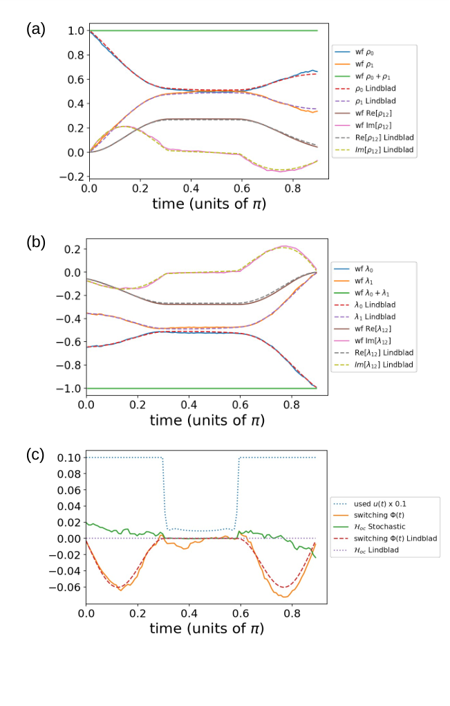
We now compute the switching functions using both procedures outlined in Section III.2. The first procedure requires the explicit constructions of the density matrix and its costates. Using the optimal control for the state retention problem [given in Fig. 1(a)], we compute $\rho$ [Eq. (16)], $\lambda$ [Eq. (18)], and thus $\Phi$ [Eq. (9)] and $\mathcal{H}_{c}$ [Eq. (10) and (13)]. The results are shown in Fig. 2 and agree well with the exact results (i.e., the results from the deterministic Lindbladian formalism). Note that in Fig. 2(c), $\Phi$ and $\mathcal{H}_{c}$ display larger errors around the switching times; we have tested that this discrepancy becomes weaker upon increasing the time points (not shown). To test the second procedure, Fig. 3 compares the switching functions computed using Eq. (22) with the exact ones. In these simulations, the non-optimal control $u(t)=-1+2\Theta(t-t_{f}/2)$ is used. A good agreement is seen for both state retention and state preparation problems, numerically confirming Eq. (22).

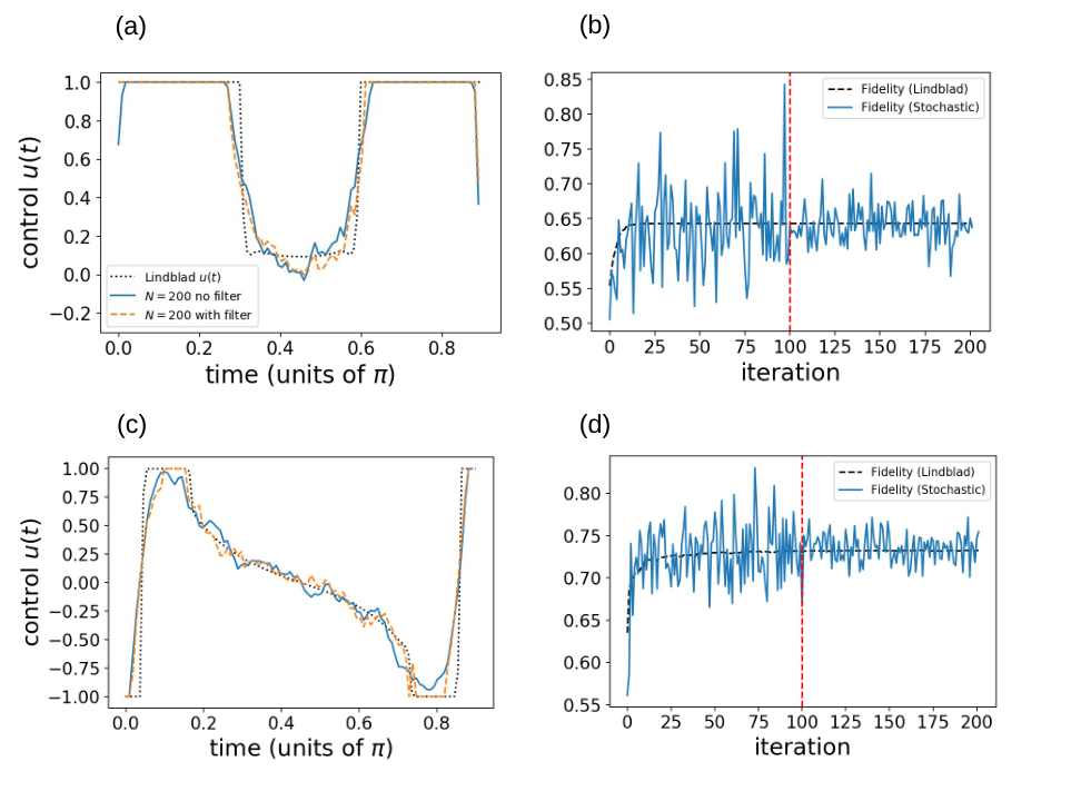
With the switching functions tested, Eq. (22) is now applied to determine the optimal control for both state retention and state preparation problems. Due to the noisy nature of stochastic simulations, filtering the functions at some point helps. After some numerical experiments, we adopt two filtering protocols: $(k+1)$th iteration is updated via

We first elaborate Eq. (26a). After $\Phi^{(k)}(t)$ is computed from Eq. (22), it is de-noised by a total-variation (TV) norm Rudin et al. 1992:

$w_{TV}=0.01$ is adopted and the proximal gradient descent is used to solve Eq. (27). We decide to regularize $\Phi(t)$ instead of $u(t)$ because TV norm tends to reduce the magnitude of the discontinuity (jump): there will be a discontinuity in $u(t)$ once $\Phi(t)$ changes sign (the bang-bang protocol) whereas $\Phi(t)$ is generally continuous. In Eq. (26b), the projection $P_{\varepsilon}$ is defined as

$\epsilon=0.1$ is used. This is designed to promote the bang control around $\Phi(t)=0$. We choose $\varepsilon=0$ in early iterations to avoid biases when $u(t)$ is still far from the optimal solution. To summarize, three optimization hyperparameters are chosen to be $(\eta,w_{TV},\varepsilon)=(0.5,0.01,0.1)$.

Left panels of Fig. 4 shows the optimal control obtained using Eq. (22) for both state retention and state preparation problems. They generally agree with the exact solutions. Compared to the solutions without filtering ($w_{TV}=\varepsilon=0$), the filtering procedure generally results in controls that are smoother over the singular regime (when $\Phi(t)=0$) and sharper near the transition regimes (when $\Phi(t)$ is changing sign or changing between zero and non-zero). Overall the controls with the filtering procedure are closer to the exact solutions. Right panels of Fig. 4 give the negative of terminal cost function (fidelity) as a function of iterations. The fidelities computed from the deterministic Lindbladian (Eq. (9), dashed curves) and the stochastic Schrödinger (Eq. (20), solid curves) formalism are numerically consistent. For the stochastic simulation, the first 100 iterations average $N=50$ realizations whereas the last 100 iterations $N=200$. The expected reduction of the fluctuation due to the larger sampling size is also clearly seen.

References

- Georgescu and Nori (2012) I. Georgescu and F. Nori, Physics World 25, 16 (2012), URL https://doi.org/10.1088%2F2058-7058%2F25%2F05%2F28.
- Nielsen and Chuang (2011) M. A. Nielsen and I. L. Chuang, Quantum Computation and Quantum Information (Cambridge University Press, Cambridge, 2011).
- Kaye et al. (2007) P. Kaye, R. Laflamme, and M. Mosca, An introduction to quantum computing (Oxford University Press, New York, 2007).
- Shor (1997) P. W. Shor, SIAM J. Comput. 26, 1484 (1997), ISSN 0097-5397.
- Grover (1996) L. K. Grover, in Proceedings of the Twenty-eighth Annual ACM Symposium on Theory of Computing (ACM, New York, 1996), pp. 212–219.
- Grover (1997) L. K. Grover, Phys. Rev. Lett. 79, 325 (1997).
- Peruzzo et al. (2014) A. Peruzzo, J. McClean, P. Shadbolt, M.-H. Yung, X.-Q. Zhou, P. J. Love, A. Aspuru-Guzik, and J. L. O’Brien, Nature Communications 5, 4213 (2014).
- Farhi et al. (2014) E. Farhi, J. Goldstone, and S. Gurmann, A quantum approximate optimization algorithm (2014), eprint arXiv:1411.4028.
- O’Malley et al. (2016) P. J. J. O’Malley, R. Babbush, I. D. Kivlichan, J. Romero, J. R. McClean, R. Barends, J. Kelly, P. Roushan, A. Tranter, N. Ding, et al., Phys. Rev. X 6, 031007 (2016), URL https://link.aps.org/doi/10.1103/PhysRevX.6.031007.
- Preskill (2018) J. Preskill, Quantum 2, 79 (2018), ISSN 2521-327X, URL https://doi.org/10.22331/q-2018-08-06-79.
- Helstrom (1976) C. W. Helstrom, Quantum Detection and Estimation Theory, Mathematics in Science and Engineering 123 (Elsevier, Academic Press, New York, 1976).
- Holevo (2011) A. S. Holevo, Probabilistic and Statistical Aspects of Quantum Theory (Edizioni della Normale, Superiore Pisa, 2011), 1st ed.
- Giovannetti et al. (2006) V. Giovannetti, S. Lloyd, and L. Maccone, Phys. Rev. Lett. 96, 010401 (2006), URL https://link.aps.org/doi/10.1103/PhysRevLett.96.010401.
- Giovannetti et al. (2011) V. Giovannetti, S. Lloyd, and L. Maccone, Nature Photonics 5, 222 (2011).
- Tsang et al. (2016) M. Tsang, R. Nair, and X.-M. Lu, Phys. Rev. X 6, 031033 (2016), URL https://link.aps.org/doi/10.1103/PhysRevX.6.031033.
- Zhuang et al. (2017) Q. Zhuang, Z. Zhang, and J. H. Shapiro, Phys. Rev. A 96, 040304 (2017), URL https://link.aps.org/doi/10.1103/PhysRevA.96.040304.
- Vahlbruch et al. (2016) H. Vahlbruch, M. Mehmet, K. Danzmann, and R. Schnabel, Phys. Rev. Lett. 117, 110801 (2016), URL https://link.aps.org/doi/10.1103/PhysRevLett.117.110801.
- Collaboration (2011) T. L. S. Collaboration, Nature Physics 7, 962 (2011).
- Sidhu and Kok (2020) J. S. Sidhu and P. Kok, AVS Quantum Science 2, 014701 (2020), URL https://doi.org/10.1116/1.5119961.
- Pezzè et al. (2018) L. Pezzè, A. Smerzi, M. K. Oberthaler, R. Schmied, and P. Treutlein, Rev. Mod. Phys. 90, 035005 (2018), URL https://link.aps.org/doi/10.1103/RevModPhys.90.035005.
- Bennett and Wiesner (1992) C. H. Bennett and S. J. Wiesner, Phys. Rev. Lett. 69, 2881 (1992), URL https://link.aps.org/doi/10.1103/PhysRevLett.69.2881.
- Braunstein and Kimble (2000) S. L. Braunstein and H. J. Kimble, Phys. Rev. A 61, 042302 (2000), URL https://link.aps.org/doi/10.1103/PhysRevA.61.042302.
- Ekert (1991) A. K. Ekert, Phys. Rev. Lett. 67, 661 (1991), URL https://link.aps.org/doi/10.1103/PhysRevLett.67.661.
- Ursin et al. (2007) R. Ursin, F. Tiefenbacher, T. Schmitt-Manderbach, H. Weier, T. Scheidl, M. Lindenthal, B. Blauensteiner, T. Jennewein, J. Perdigues, P. Trojek, et al., Nature Physics 3, 481 (2007).
- Caves and Drummond (1994) C. M. Caves and P. D. Drummond, Rev. Mod. Phys. 66, 481 (1994), URL https://link.aps.org/doi/10.1103/RevModPhys.66.481.
- Braunstein and van Loock (2005) S. L. Braunstein and P. van Loock, Rev. Mod. Phys. 77, 513 (2005), URL https://link.aps.org/doi/10.1103/RevModPhys.77.513.
- Weedbrook et al. (2012) C. Weedbrook, S. Pirandola, R. García-Patrón, N. J. Cerf, T. C. Ralph, J. H. Shapiro, and S. Lloyd, Rev. Mod. Phys. 84, 621 (2012), URL https://link.aps.org/doi/10.1103/RevModPhys.84.621.
- Bao et al. (2018) S. Bao, S. Kleer, R. Wang, and A. Rahmani, Phys. Rev. A 97, 062343 (2018).
- Omran et al. (2019) A. Omran, H. Levine, A. Keesling, G. Semeghini, T. T. Wang, S. Ebadi, H. Bernien, A. S. Zibrov, H. Pichler, S. Choi, et al., Science 365, 570 (2019).
- Friis et al. (2018) N. Friis, O. Marty, C. Maier, C. Hempel, M. Holzäpfel, P. Jurcevic, M. B. Plenio, M. Huber, C. Roos, R. Blatt, et al., Phys. Rev. X 8, 021012 (2018).
- Doherty et al. (2014) M. W. Doherty, V. V. Struzhkin, D. A. Simpson, L. P. McGuinness, Y. Meng, A. Stacey, T. J. Karle, R. J. Hemley, N. B. Manson, L. C. L. Hollenberg, et al., Phys. Rev. Lett. 112, 047601 (2014).
- Farhi et al. (2000) E. Farhi, J. Goldstone, S. Gurmann, and M. Sipser, Quantum computation by adiabatic evolution (2000), eprint arXiv:quant-ph/0001106.
- Rezakhani et al. (2009) A. T. Rezakhani, W.-J. Kuo, A. Hamma, D. A. Lidar, and P. Zanardi, Phys. Rev. Lett. 103, 080502 (2009), URL https://link.aps.org/doi/10.1103/PhysRevLett.103.080502.
- Zhuang (2014) Q. Zhuang, Phys. Rev. A 90, 052317 (2014), URL https://link.aps.org/doi/10.1103/PhysRevA.90.052317.
- Haine and Hope (2020) S. A. Haine and J. J. Hope, Phys. Rev. Lett. 124, 060402 (2020), URL https://link.aps.org/doi/10.1103/PhysRevLett.124.060402.
- Pontryagin (1987) L. Pontryagin, Mathematical Theory of Optimal Processes (CRC Press, Boca Raton, FL, 1987).
- Sussmann (1987) H. J. Sussmann, SIAM Journal on Control and Optimization 25, 433 (1987).
- Luenberger (1979) D. G. Luenberger, Introduction to dynamic systems: theory, models, and applications (Wiley, New York, 1979).
- Heinz Schattler (2012) U. L. Heinz Schattler, Geometric Optimal Control: Theory, Methods and Examples, Interdisciplinary Applied Mathematics 38 (Springer-Verlag, New York, 2012), 1st ed., ISBN 978-1-4614-3833-5,978-1-4614-3834-2.
- Lin et al. (2020) C. Lin, D. Sels, and Y. Wang, Phys. Rev. A 101, 022320 (2020).
- Yang et al. (2017) Z.-C. Yang, A. Rahmani, A. Shabani, H. Neven, and C. Chamon, Phys. Rev. X 7, 021027 (2017).
- Lin et al. (2019) C. Lin, Y. Wang, G. Kolesov, and U. Kalabic, Phys. Rev. A 100, 022327 (2019).
- Zeng and Barnes (2018) J. Zeng and E. Barnes, Phys. Rev. A 98, 012301 (2018).
- Hegerfeldt (2013) G. C. Hegerfeldt, Phys. Rev. Lett. 111, 260501 (2013).
- Bukov et al. (2018) M. Bukov, A. G. R. Day, D. Sels, P. Weinberg, A. Polkovnikov, and P. Mehta, Phys. Rev. X 8, 031086 (2018).
- Sugny et al. (2007) D. Sugny, C. Kontz, and H. R. Jauslin, Phys. Rev. A 76, 023419 (2007), URL https://link.aps.org/doi/10.1103/PhysRevA.76.023419.
- Wang et al. (2008) L. C. Wang, X. L. Huang, and X. X. Yi, Phys. Rev. A 78, 052112 (2008), URL https://link.aps.org/doi/10.1103/PhysRevA.78.052112.
- Stefanatos (2009) D. Stefanatos, Phys. Rev. A 80, 045401 (2009), URL https://link.aps.org/doi/10.1103/PhysRevA.80.045401.
- Ritland and Rahmani (2018) K. Ritland and A. Rahmani, New Journal of Physics 20, 065005 (2018), URL https://doi.org/10.1088%2F1367-2630%2Faaca62.
- Deutsch and Jozsa (1992) D. Deutsch and R. Jozsa, Proceedings of the Royal Society of London. Series A: Mathematical and Physical Sciences 439, 553 (1992).
- Simon (1997) D. R. Simon, SIAM J. Comput. 26, 1474 (1997), ISSN 0097-5397, URL http://dx.doi.org/10.1137/S0097539796298637.
- Bennett et al. (1997) C. Bennett, E. Bernstein, G. Brassard, and U. Vazirani, SIAM Journal on Computing 26, 1510 (1997).
- Harrow et al. (2009) A. W. Harrow, A. Hassidim, and S. Lloyd, Phys. Rev. Lett. 103, 150502 (2009), URL https://link.aps.org/doi/10.1103/PhysRevLett.103.150502.
- Shor (1995) P. W. Shor, Phys. Rev. A 52, R2493 (1995), URL https://link.aps.org/doi/10.1103/PhysRevA.52.R2493.
- Steane (1996) A. M. Steane, Phys. Rev. Lett. 77, 793 (1996), URL https://link.aps.org/doi/10.1103/PhysRevLett.77.793.
- Knill and Laflamme (1997) E. Knill and R. Laflamme, Phys. Rev. A 55, 900 (1997), URL https://link.aps.org/doi/10.1103/PhysRevA.55.900.
- Gottesman (1997) D. Gottesman, Stabilizer codes and quantum error correction (1997), eprint arXiv:quant-ph/9705052.
- Hirose and Cappellaro (2016) M. Hirose and P. Cappellaro, Nature 532, 77 (2016).
- Viola and Lloyd (1998) L. Viola and S. Lloyd, Phys. Rev. A 58, 2733 (1998), URL https://link.aps.org/doi/10.1103/PhysRevA.58.2733.
- Viola et al. (1999) L. Viola, E. Knill, and S. Lloyd, Phys. Rev. Lett. 82, 2417 (1999), URL https://link.aps.org/doi/10.1103/PhysRevLett.82.2417.
- Benedetti et al. (2013) C. Benedetti, F. Buscemi, P. Bordone, and M. G. A. Paris, Phys. Rev. A 87, 052328 (2013), URL https://link.aps.org/doi/10.1103/PhysRevA.87.052328.
- Uhlmann (1976) A. Uhlmann, Reports on Mathematical Physics 9, 273 (1976), ISSN 0034-4877, URL http://www.sciencedirect.com/science/article/pii/0034487776900604.
- Jozsa (1994) R. Jozsa, Journal of Modern Optics 41, 2315 (1994).
- (64) The control Hamiltonian is defined as the inner product of a costate and the time-derivative of the state . The space of matrices forms a Hilbert space, and adopting the Hilbert-Schmidt inner product immediately leads to Eq. (4). Alst note that when and are Hermitian and the dynamics is a proper completely positive and trace-preserving map, Tr is guaranteed to be real.
- Breuer and Petruccione (2002) H.-P. Breuer and F. Petruccione, The Theory of Open Quantum Systems (Oxford University Press, 2002).
- Dalibard et al. (1992) J. Dalibard, Y. Castin, and K. Mølmer, Phys. Rev. Lett. 68, 580 (1992), URL https://link.aps.org/doi/10.1103/PhysRevLett.68.580.
- Castin et al. (2008) Y. Castin, J. Dalibard, and K. Molmer, A wave function approach to dissipative processes (2008), eprint 0805.4002.
- Rudin et al. (1992) L. I. Rudin, S. Osher, and E. Fatemi, Physica D: Nonlinear Phenomena 60, 259 (1992), ISSN 0167-2789, URL http://www.sciencedirect.com/science/article/pii/016727899290242F.