Beating classical heuristics for the binary paint shop problem with the quantum approximate optimization algorithmPreprint: APS/123-QED
Abstract
The binary paint shop problem (BPSP) is an APX-hard optimization problem of the automotive industry. In this work, we show how to use the Quantum Approximate Optimization Algorithm (QAOA) to find solutions of the BPSP. We demonstrate that QAOA with constant depth is able to beat all known heuristics for the binary paint shop problem on average in the infinite size limit . We complete our studies by running first experiments of small-sized instances on a trapped-ion quantum computer through Amazon Braket.
I Introduction
Achievements in fabrication and control of two-level systems led to first quantum computers with tens of qubits Barends et al. 2016; DiCarlo et al. 2009; Debnath et al. 2016; Reagor et al. 2018 and recently culminated in the demonstration of a quantum computer solving a computational task intractable for classical computers, also known as quantum supremacy Arute et al. 2019. This milestone raises expectations that quantum computing some day will accelerate research, speed up simulations in chemistry and improve optimization processes in many branches of industry. Quantum algorithms with proven scaling advantage over classical algorithms, such as Grover’s Grover 1996 or Shor’s Shor 1994 algorithm, require fault-tolerant quantum computers. However the devices which will become available in the next 5 to 10 years will only have a limited number of qubits and will not feature error-correction. It is unclear if such Noisy Intermediate-Scale Quantum (NISQ) devices can be useful in solving real-world problems faster than classical computers or if larger error-corrected devices will be needed. To answer this question it is especially important to develop quantum algorithms tailor-made to the quantum processing units’ (QPU) characteristics. A promising class of NISQ algorithms is the class of variational quantum algorithms, which are parameterized ansätze optimized with classical learning loops. There exist various ideas how to tailor the ansatz for different tasks, such as the Variational Quantum Eigensolver (VQE) for chemistry applications Peruzzo et al. 2014 or Quantum Neural Networks (QNN) for machine learning Mitarai et al. 2018; Killoran et al. 2019. The QAOA is a variational algorithm designed to solve classical optimization problems Farhi et al. 2014 and was applied to problems such as Max-Cut Farhi et al. 2014 or Max-3-Lin-2 Farhi et al. 2014. Furthermore, there exist first insights on QAOAs performance Crooks 2018; Streif and Leib 2019; Streif and Leib 2020a; Willsch et al. 2020, first experimental realizations on different quantum processors Arute et al. 2020; Pagano et al. 2020; Otterbach et al. 2017 and several proposals how to further improve QAOA Zhou et al. 2020; Mbeng et al. 2019; Bapat and Jordan 2018; Hastings 2019; Bravyi et al. 2019a; Brandao et al. 2018; Streif and Leib 2020b. For example in Streif and Leib 2020b, it was shown that for some problem classes with certain topological characteristics it is possible to find good parameters for QAOA with classical methods efficiently. Moreover, there exist results showing that it is classically hard to sample from the QAOA output Farhi and Harrow 2016 and that QAOA possesses a Grover-type speed-up Jiang et al. 2017. However, performance bounds are only known for very short circuits Farhi et al. 2014 or classically easy instances Mbeng et al. 2019. Establishing scaling comparisons, beyond low depth circuits, between QAOA and classical methods for application relevant optimization problems is the next important step to find useful NISQ applications of QAOA.
In this present contribution, we take a step in this direction using the example of a combinatorial optimization problem from the automotive industry, the binary paint shop problem (BPSP). We show that the problem can be encoded into a spin glass in a constraint-free way and requires only linear number of qubits for increasing problem size. As such it is a perfect fit for QAOA on NISQ devices. We show that the problem has fixed degree and coupling strength, which allows us to use the method developed in Streif and Leib 2020b which bypasses the NP-hard training procedure Bittel and Kliesch 2021. We present numerical results and run first small-scale experiments on a trapped ion quantum computer. We are numerically able to prove a minimal depth for QAOA to beat classical heuristics in the small to medium system size limit (up to 100 cars) as well as for the infinite size limit. With this we show that a constant time quantum algorithm can beat a polynomial time classical algorithm.
This paper is structured as follows. In Sec. II we review the Quantum Approximate Optimization Algorithm (QAOA). In Sec. III we review the binary paint shop problem, classical greedy algorithms to solve it and discuss the mapping of the problem onto an Ising Hamiltonian. In Sec. IV we show results of QAOA applied to the BPSP and in Sec. V, we conclude.
II Review of QAOA
In this section, we review the Quantum Approximate Optimization Algorithm (QAOA) Farhi et al. 2014, a variational quantum algorithm designed to solve combinatorial optimization problems.
To solve a combinatorial optimization problem with QAOA, the first step is to reformulate it as a spin glass problem. For our purposes the spin glass can be represented as a problem graph with nodes representing spins and edges representing the terms of the sum of the energy of the spin glass that needs to be minimized. We note that finding the optimal solution of a spin glass is -hard Barahona 1982, thus there exist mappings with at most polynomial overhead from all problems to such a spin system, some of them shown in Lucas 2014. We search for low energy configurations of the spin glass with a variational ansatz. In QAOA, this is done by minimizing the expectation value of the problem Hamiltonian with respect to a parameterized ansatz state ,
| (1) |
Therefore we translate the spin system to its quantum version
| (2) |
where each classical spin variable is replaced by a qubit with the Pauli-Z operator . The ansatz state in QAOA is inspired by quantum annealing techniques and is generated by the repeated application of the mixing and problem unitary, and , on the superposition state of all computational basis states, . The generators of these unitaries are given by the mixing Hamiltonian, , and the problem Hamiltonian, see Eq. (2). The full ansatz state
| (3) |
includes repetition of those unitaries, where each repetition is called a QAOA level. To find the optimal variational parameters , a quantum computer is used to estimate the expectation value of the problem Hamiltonian, while an outer learning loop on a classical computer updates the parameters to minimize the expectation value. Recent work has shown how to speed up the classical learning loop Zhou et al. 2020 or alternatively using entirely classical methods to find optimal parameters for certain problem classes Streif and Leib 2020b. Having found the optimal parameters, one then samples from the final state in the computational basis which yields solutions to the optimization problem.
III The binary paint shop problem
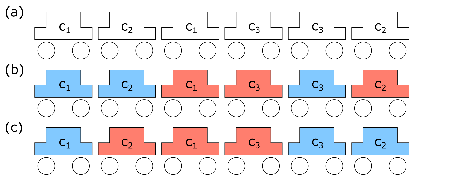
Assume an automotive paint shop and a random, but fixed sequence of cars. The task is to paint the cars in the order given by the sequence. Each individual car needs to be painted with two colors, once per color, in a to-be-determined color order. Meaning, each car appears twice at random, uncorrelated positions in the sequence and we are free to choose the color to paint the car first. A specific choice of first colors for every car is called a coloring. The objective of the optimization problem is to find a coloring which minimizes the number of color changes between adjacent cars in the sequence. This combinatorial optimization problem is called the binary paint shop problem (BPSP) Epping et al. 2001; Epping et al. 2004; Gupta et al. 2013. In Fig. 1, we show a binary paint shop instance together with a sub-optimal and the optimal solution. A formal definition of the binary paint shop problem is given in Def. III.1.
Definition III.1.
(Binary paint shop problem) Let be the set of cars . An instance of the binary paint shop problem is given by a sequence with , where each car appears exactly twice. We are given two colors . A coloring is a sequence with and if for . The objective is to minimize the number of color changes .
The binary paint shop problem belongs to the class of -hard optimization problems, thus there is no polynomial-time algorithm which finds the optimal solution for all problem instances. For many optimization problems in practice, rather than spending exponential time to find the optimal solution, fast approximate algorithms are used. However, the binary paint shop problem is proven to be -hard Epping et al. 2004, i.e. it is as difficult to approximate as every problem in . Additionally, if the Unique Games Conjecture (UGC) Khot 2002 holds, it is even not in and thus, there would not be a constant factor approximation algorithm for any Gupta et al. 2013. A constant factor approximation algorithm would be a polynomial-time algorithm which returns an approximate solution with at most color changes where is the optimal number of color changes. This is a key difference to previous problem classes QAOA has been applied to, such as Max-Cut, where constant factor approximation algorithms are known Goemans and Williamson 1995.
Several greedy algorithms exist for the binary paint shop problem which provide solutions with color changes linear in the number of cars on average Epping et al. 2004; Epping et al. 2001. The greedy algorithm introduced in Epping et al. 2001 starts at the first car of the sequence with one of both colors, goes through the sequence and changes colors when necessary, i.e. only if the same car would be painted twice with the same color, see Fig. 2 for pseudo code of this algorithm. For cars, this greedy algorithm finds a solution with an average number of color changes Andres and Hochstättler 2011. In Appendix A, we review two other greedy algorithms, the red first algorithm and the recursive greedy algorithm, yielding and color changes on average respectively Andres and Hochstättler 2011. Numerical results however suggest that the average number of optimal color changes is sub-linear in the number of cars Meunier and Neveu 2012. Moreover, for some instances, the greedy algorithms only find solutions far from the optimal solution Andres and Hochstättler 2011. For example, for the instance shown in Fig. 1(a), the greedy algorithm finds the solution given in (b) rather then the optimal solution shown in (c).
More general versions of the binary paint shop problem can be found in practice. Typically both the color set is augmented to contain more than two colors, and identical cars appear more than twice per word. These conditions correspond to the real-world application of painting thousands of car bodies per day, with numerous colors. Even restricting the color set to two colors has real-world relevance: before painting the final color of the body, each car is first painted with an undercoat called a filler coat. The filler colors are restricted to white and black, depending on the final car body color, and optimizing the number of color switches within the filler queue yields production cost savings. Given that the generalized paint shop problem is -hard in both the number of cars and colors Epping et al. 2004, and that the binary color set is already industrially relevant, we restrict the color set to two colors in this study.
III.1 Reformulating the BPSP as a spin glass
In this section, we explain how to map the binary paint shop problem to a problem Hamiltonian as in Eq. (2).
We start by assigning a single qubit to each car in the sequence. The eigenstates of the -operator of each qubit indicate in which color each car is painted first. The second color choice for each car in the sequence is then unambiguously determined. To penalize color changes in the coloring, we use the coupling strengths between the qubits. We start at the first car in the sequence and step through the sequence adding couplings between the qubits representing the car and its next neighbor in the sequence. If both cars and , represented by and respectively, appear both for the first or second time, a ferromagnetic coupling, , is added. This ensures that consecutive cars favor to be painted with the same color. If either car has already appeared in the sequence while the other has not, we instead add an antiferromagnetic coupling, . We know that a solution with color changes is separated by an energy from a solution with color changes. We show pseudo code of this mapping in Fig. 3. We note that the encoding of the problem does not include any constraints, thus all computational states embody valid solutions to the problem. Moreover, the encoding only requires qubits for cars, making it a better fit for NISQ devices than typical scheduling problems (like the traveling salesman problem) where the number of qubits required grows quadratically with the system size Lucas 2014. From the BPSP construction, we also know that a solution with color changes is separated by an energy from a solution with color changes.
III.1.1 Properties of the Ising Hamiltonian
In Streif and Leib 2020b it was shown how to calculate close-to-optimal QAOA parameters using a classical computer for various levels , and problem classes represented by graphs with fixed degree and uniform coupling strengths, . For the NISQ era, where typically is small, this method circumvents optimizing the variational parameters of the QAOA ansatz state for each instance independently, and thus reduces the total QPU time used. In this section, we show that the binary paint shop instances represent graphs of fixed and average degree and coupling strengths (both for ). As this method originally was proposed for the case only, we prove in Appendix C that the method also works if . In the following we argue that the BPSP is a perfect fit for parameters calculated using this method.
Average degree
In the construction of the problem Hamiltonian, cf. Sec. III.1, we add an interaction between two qubits if the corresponding cars are adjacent. As each car only appears times, each car has maximal distinct neighbors. It follows that the nodes in the graph representing the spin system also have maximal degree of . The degree is only smaller than for the node representing the first or the last car in the sequence, or if the car is adjacent to the same car twice. In Fig. 7(a), we show that the average degree of the graph is converging to from below and becomes effectively -regular when .
Coupling strengths
From the construction of the Ising Hamiltonian, we also know that the interaction values are integers and given by . In Appendix B, we show that the distribution of interaction values converges to a distribution with and , when . This means that the probability of a ferromagnetic coupling is twice as big as for an anti-ferromagnetic coupling and that coupling strengths are suppressed in the infinite size limit. We note however that the coupling strengths are not independent from each other.
IV Solving the Binary Paint Shop problem with QAOA
In the following sections, we apply QAOA to the binary paint shop problem. For all simulations and experiments, we use the parameters found with method Streif and Leib 2020b, shown in Tab. 2.
IV.1 Numerical results
In this section, we numerically analyze the performance of QAOA on randomly generated binary paint shop instances of sizes from to cars in increments of cars bps.
For up to cars we calculate the QAOA output state, Eq. (3) for levels of QAOA and determine the energy expectation value Eq. (1) together with the expected number of color changes . For larger systems, the calculation of the QAOA output state is out of reach using a standard desktop computer.
However, since we are only interested in the energy expectation value and not in the output state, we use a proxy to calculate the expectation value for small values of . First, we rewrite Eq. (1) as a sum over all expectation values of two-point correlation functions,
| (4) |
As pointed out in Farhi et al. 2014; Streif and Leib 2020b, the individual expectation values do not necessarily depend on the states of all qubits, but only on a subset, which can be used to reduce the computational cost to calculate them. Some of the gates defined in commute with the operator product , and since the gates are unitary we can completely skip them in the definition of the correlation function,
| (5) |
where is the set of gates not commuting with called the reverse causal cone of the correlation function, is the support of the reverse causal cone, i.e. the minimal set of qubits the reverse causal cone acts on, and is the superposition state of all computational basis states of the qubits in the reverse causal cone. The support of the reverse causal cone can be constructed in an iterative procedure Farhi et al. 2014; Streif and Leib 2020b: for each layer in the QAOA circuit we add all new neighbors in the problem graph of the support of the reverse causal cone of a QAOA circuit with one level less starting with the two qubits that define the correlation function. Therefore, the number of qubits affecting the expectation value depends on the number of QAOA levels and the topology of the problem. The binary paint shop instances can be represented as graphs with bounded degree of , thus the reverse causal cone includes up to qubits. For this results in system sizes that can be simulated using a standard desktop computer, independent of the actual size of the instance. After calculating the individual correlation functions independently we find the QAOA expectation value by using Eq. (4).
In Fig. 4, we show the expected color changes from the QAOA output averaged over all instances together with the average result of the greedy algorithm, see Fig. 2, and exact solutions for up to cars. Low-depth QAOA with performs worse than the polynomial-time greedy algorithm, while for levels the performance gap nearly vanishes. For QAOA outperforms the greedy algorithm.
IV.2 Beating the greedy algorithms for large instances
The greedy algorithms presented in Sec. III provide solutions with color changes growing linearly with the number of cars on average in polynomial time. Thus, they provide a good performance benchmark for QAOA. In Sec. IV.1, numerical simulations revealed that QAOA with fixed level is able to beat the greedy algorithm on average. In this section, we strengthen this result with numerical insights in the infinite size limit, .
To understand the performance of the greedy algorithm it is instructive to translate the action of the greedy algorithm presented in Fig. 2 into the spin glass picture. For the sake of clarity of presentation, we assume that all couplings have magnitude , which is true in the infinite size limit. The greedy algorithm starts with assigning a random configuration to the spin representing the first car of the sequence. It then successively visits the spins representing the next car in the sequence. If it visits a car for the first time, it fixes the state of its spin such that the coupling between the car and its predecessor is fulfilled, i.e. same state for ferromagnetic- and opposite state for antiferromagnetic coupling.
The greedy algorithm is guaranteed to satisfy a coupling every time it approaches a spin representing a car that has not been visited yet. This happens times. The remaining connections in the full graph are, however, not taken into account. On average, the energy of these unseen connections is equal to zero. In total, for , the greedy algorithm generates a solution with average energy of , which results in solutions with color changes growing according to .
In comparison, in the limit of , the reverse causal cones of the two-point correlation functions after levels of QAOA only include qubits in graphs which resemble trees of degree and coupling strengths (see Appendix B). Thus, for systems of infinite size, the expectation value of each two-local operator is the same on average and given by the expectation value calculated on a tree.
To calculate the expectation value with a state-vector simulation, we would have to include qubits, which is difficult to calculate classically even for shallow versions of QAOA. In Streif and Leib 2020b, the authors developed a method that substantially increases the simulation capabilities using the small tree width of the involved tensor networks Markov and Shi 2008. To calculate the two-point correlation functions on tree subgraph support, this method only scales polynomially in the number of qubits, but exponentially in the number of QAOA blocks. This allows us to calculate the expectation value up to levels of QAOA, including qubits. With that we find average energies and color changes given in Tab. 1. We note that the tensor network calculation also requires the optimization of the QAOA parameters. As the optimization might have found a local optimum rather than the global optimum, the values in Tab. 1 for QAOA represent lower bounds on the performance. If one would be able to find a better set of parameters, the performance of the algorithm could be even improved.
We recognize that the performance of QAOA with levels is close to the performance of the greedy algorithm, while for there is a clear performance gap in favor of QAOA. While these arguments strictly hold for the limit of , we have shown that the results on smaller systems (see Fig. 4) agree with these results. When comparing the performance to two other heuristics, the red-first algorithm and the recursive greedy algorithm (see Appendix A), we see that QAOA outperforms the red-first algorithm on average with levels and for QAOA also beats the recursive greedy algorithm on average. In Fig. 5, we show the data plotted against the number of QAOA blocks together with a fit highlighting the improvement in performance when increasing .
To determine the run time of the quantum algorithm on a state-of-the-art quantum processing unit we recall that the binary paint shop problem can be represented as a graph of maximal degree 4 (see Sec. III.1.1). On a fully-connected quantum computer, the corresponding QAOA circuit with a fixed value of thus only requires constant depth, making the QAOA for the BPSP a constant-time algorithm. This is in contrast with classical algorithms, which are polynomial-time algorithms. On quantum hardware with limited topology, e.g. for superconducting qubit devices with planar connectivity graphs, one could use methods such as the LHZ-encoding Lechner 2018, which require a quadratic overhead in qubits, however still have constant computing time.
| Method | |
|---|---|
| Random guessing | 1.000 |
| p=1 | 0.675 |
| Red first algorithm | 0.666 |
| p=2 | 0.568 |
| p=3 | 0.503 |
| Greedy algorithm, see Fig. 2 | 0.500 |
| p=4 | 0.462 |
| p=5 | 0.432 |
| p=6 | 0.411 |
| Recursive greedy algorithm | 0.400 |
| p=7 | 0.393 |
IV.3 Experimental results
In this section, we show the results from QAOA circuits of binary paint shop instances with executed on a trapped-ion quantum computer, the IonQ device Wright et al. 2019, provided by Amazon Braket AWS. This device is composed of fully-connected qubits with average single- and two-qubit fidelities of and respectively Wright et al. 2019.
Like most available quantum hardware, trapped ion quantum computers only allow the application of gates from a restricted native gate set predetermined by the physical realization of the processor. To execute an arbitrary gate, compilation of the desired gate into available gates is required. For trapped ions, a generic native gate set consists of a parameterized two-qubit rotation, on qubits and , and a single qubit rotation, ,
| (6) |
which includes and Maslov 2017. These gates form a universal set of gates, i.e. all other gates can be synthesized with these gates.
The QAOA circuit, defined in Eq. (3), includes the parameterized two-qubit rotation on qubits and , parameterized single qubit rotations and Hadamard gates. While the local is readily available on the hardware and can be executed without any overhead, the Hadamard gate and the two-qubit rotation require compilation which will in turn increase the circuit depth.
To make the circuit as short as possible, we rotate the circuit by inserting Hadamard gates. For the sake of clarity, we introduce the unitary , which highlights that the problem unitary is a set of gates. Accordingly, is the unitary in which all in were replaced by gates. The same pattern applies for the definition of the mixing unitary , i.e. denotes an unitary where all gates are replaced by gates. The new circuit,
| (7) |
then only contains gates from the native gate set and thus needs no further compilation. For higher -value, the transformation is analogous and shown in Appendix D.
On IonQ devices, all gates are executed in sequence ion. Thus, this representation of a QAOA circuit of a binary paint shop instance with nodes and edges can be carried out with circuit depth and requires single qubit gates and two-qubit gates. As the binary paint shop instances are bounded degree graphs with maximal degree 4, cf. Sec. III.1.1, the circuit depth scales linearly with the system size , .
We execute the QAOA circuit with for randomly drawn binary paint shop instances from to cars bps. For each instance, we take samples and calculate the average number of color changes, . For comparison, we take data from an ideal (noiseless) simulation and random guessing. To compare the experimental output with the ideal simulation and random guessing, we calculate the deviation in performance as
| (8) |
where , and denote the expected instance-wise color change obtained from the simulation, the QPU and random guessing respectively. A value of implies that the QPU found results as good as the ideal simulation did, while means that the QPU output mimics random guessing.
In Fig. 6, we plot the distribution of over all instances for increasing system size. As clearly visible, for the smallest system size () the results are close to an ideal simulation, while for the largest studied instances (), the output is almost random. Similar to previous QAOA experiments Arute et al. 2020; Pagano et al. 2020; Otterbach et al. 2017, the present results highlight the strong influence of noise on the performance of the quantum algorithm. Moreover, in the same figure, we show the quantity where we replaced the QPU results with obtained from a simulation with noise. In this simulation, the noise was tuned such that we find agreement with the reported single- and two-qubit fidelities in Wright et al. 2019. For more details on the noise model used, we refer to Appendix E. As visible, the simulation with noise cannot fully explain the experimental data. This could have several reasons:
- 1.
On IonQ all gates are carried out strictly successively ion, which leads to long idle times of the qubits. This is not taken into account by errors of single- and two-qubit gates.
- 2.
The fidelites reported in Wright et al. 2019 were obtained for isolated 1- and 2-qubit gates.
This outcome highlights that single- and two-qubit fidelities are not sufficient to fully characteristic the hardware’s performance.
V Conclusion & Outlook
In this work, we applied QAOA to the binary paint shop problem, a computational problem from the automotive industry. We have shown numerical simulations together with experimental data obtained from a trapped ion quantum computer. Moreover, we were able to provide a comparison between the performance of QAOA and classical heuristics in the infinite size limit for noiseless quantum computation.
The experimental results of this paper highlight the deterioration of the quantum algorithm’s performance when increasing the problem size. To push forward to industry-relevant binary paint shop instances with hundreds of cars, either noise mitigation techniques or adaptions of QAOA must be developed to make this application on NISQ devices superior to random guessing. In this direction, the recursive adaption of QAOA introduced in Bravyi et al. 2019b or the encoding of QAOA into a lattice gauge model Lechner 2018 might provide improvements. Moreover, it would be interesting to investigate whether classical local algorithms Hastings 2019 are able to outperform the here shown results and to improve the classical performance bounds.
Furthermore, providing an answer on the question whether QAOA is a constant factor approximation algorithm could open up new room for quantum advantage.
This work has impact far beyond the restricted use case of the binary paint shop. In the way the binary paint shop problem is formulated we can already see that it is more general: every re-sequencing problem with a cost function that only depends on the relative orientation of variables that are adjacent in the sequence is similar to the binary paint shop problem. Even a generalization to next-to adjacent orientation is straightforward. These kind of re-sequencing problems are prevalent in many production facilities. For example the optimisation problem of cars being assembled by workers: cars with sunroofs are more difficult to assemble and should not be adjacent in a sequence so that the workers can keep up with the constant speed of the conveyor belt. Furthermore, since we use a generic quantum algorithm, QAOA, we are confident that the observed runtime and solution quality enhancements will prevail as long as we do not change the general problem characteristics: regular problem graph with interaction strengths of magnitude 1. These strict requirements can also be relaxed to a considerable amount as shown in Streif and Leib 2020b. We relegate the search for interesting use-cases within this group to future work.
Acknowledgements.
This project has received funding from the European Union’s Horizon 2020 research and innovation programme under the Grant Agreement No. 828826. We thank Martin Schütz for technical support with Amazon Braket and Héctor Valverde for technical support with AWS.References
- Barends et al. (2016) R. Barends, A. Shabani, L. Lamata, J. Kelly, A. Mezzacapo, U. Las Heras, R. Babbush, A. G. Fowler, B. Campbell, Y. Chen, et al., Digitized adiabatic quantum computing with a superconducting circuit, Nature 534, 222 (2016).
- DiCarlo et al. (2009) L. DiCarlo, J. Chow, J. Gambetta, L. S. Bishop, B. Johnson, D. Schuster, J. Majer, A. Blais, L. Frunzio, S. Girvin, et al., Demonstration of two-qubit algorithms with a superconducting quantum processor, Nature 460, 240 (2009).
- Debnath et al. (2016) S. Debnath, N. M. Linke, C. Figgatt, K. A. Landsman, K. Wright, and C. Monroe, Demonstration of a small programmable quantum computer with atomic qubits, Nature 536, 63 (2016).
- Reagor et al. (2018) M. Reagor, C. B. Osborn, N. Tezak, A. Staley, G. Prawiroatmodjo, M. Scheer, N. Alidoust, E. A. Sete, N. Didier, M. P. da Silva, et al., Demonstration of universal parametric entangling gates on a multi-qubit lattice, Science advances 4, eaao3603 (2018).
- Arute et al. (2019) F. Arute, K. Arya, R. Babbush, D. Bacon, J. C. Bardin, R. Barends, R. Biswas, S. Boixo, F. G. Brandao, D. A. Buell, et al., Quantum supremacy using a programmable superconducting processor, Nature 574, 505 (2019).
- Grover (1996) L. K. Grover, A fast quantum mechanical algorithm for database search, arXiv preprint quant-ph/9605043 (1996).
- Shor (1994) P. W. Shor, Algorithms for quantum computation: Discrete logarithms and factoring, in Proceedings 35th annual symposium on foundations of computer science (IEEE, 1994) pp. 124–134.
- Peruzzo et al. (2014) A. Peruzzo, J. McClean, P. Shadbolt, M.-H. Yung, X.-Q. Zhou, P. J. Love, A. Aspuru-Guzik, and J. L. O’brien, A variational eigenvalue solver on a photonic quantum processor, Nature communications 5, 4213 (2014).
- Mitarai et al. (2018) K. Mitarai, M. Negoro, M. Kitagawa, and K. Fujii, Quantum circuit learning, Physical Review A 98, 032309 (2018).
- Killoran et al. (2019) N. Killoran, T. R. Bromley, J. M. Arrazola, M. Schuld, N. Quesada, and S. Lloyd, Continuous-variable quantum neural networks, Physical Review Research 1, 033063 (2019).
- Farhi et al. (2014) E. Farhi, J. Goldstone, and S. Gutmann, A quantum approximate optimization algorithm, arXiv preprint arXiv:1411.4028 (2014).
- Farhi et al. (2014) E. Farhi, J. Goldstone, and S. Gutmann, A quantum approximate optimization algorithm applied to a bounded occurrence constraint problem, arXiv preprint arXiv::1412.6062 (2014).
- Crooks (2018) G. E. Crooks, Performance of the quantum approximate optimization algorithm on the maximum cut problem, arXiv preprint arXiv:1811.08419 (2018).
- Streif and Leib (2019) M. Streif and M. Leib, Comparison of QAOA with quantum and simulated annealing, arXiv preprint arXiv:1901.01903 (2019).
- Streif and Leib (2020a) M. Streif and M. Leib, Forbidden subspaces for level-1 quantum approximate optimization algorithm and instantaneous quantum polynomial circuits, Physical Review A 102, 042416 (2020a).
- Willsch et al. (2020) M. Willsch, D. Willsch, F. Jin, H. De Raedt, and K. Michielsen, Benchmarking the quantum approximate optimization algorithm, Quantum Information Processing 19, 197 (2020).
- Arute et al. (2020) F. Arute, K. Arya, R. Babbush, D. Bacon, J. C. Bardin, R. Barends, S. Boixo, M. Broughton, B. B. Buckley, D. A. Buell, et al., Quantum approximate optimization of non-planar graph problems on a planar superconducting processor, arXiv preprint arXiv:2004.04197 (2020).
- Pagano et al. (2020) G. Pagano, A. Bapat, P. Becker, K. S. Collins, A. De, P. W. Hess, H. B. Kaplan, A. Kyprianidis, W. L. Tan, C. Baldwin, et al., Quantum approximate optimization of the long-range ising model with a trapped-ion quantum simulator, Proceedings of the National Academy of Sciences 117, 25396 (2020).
- Otterbach et al. (2017) J. Otterbach, R. Manenti, N. Alidoust, A. Bestwick, M. Block, B. Bloom, S. Caldwell, N. Didier, E. S. Fried, S. Hong, et al., Unsupervised machine learning on a hybrid quantum computer, arXiv preprint arXiv:1712.05771 (2017).
- Zhou et al. (2020) L. Zhou, S.-T. Wang, S. Choi, H. Pichler, and M. D. Lukin, Quantum approximate optimization algorithm: Performance, mechanism, and implementation on near-term devices, Physical Review X 10, 021067 (2020).
- Mbeng et al. (2019) G. B. Mbeng, R. Fazio, and G. Santoro, Quantum annealing: a journey through digitalitalization, control, and hybrid quantum variational schemes, arXiv preprint arXiv:1906.08948 (2019).
- Bapat and Jordan (2018) A. Bapat and S. Jordan, Bang-bang control as a design principle for classical and quantum optimization algorithms, arXiv preprint arXiv:1812.02746 (2018).
- Hastings (2019) M. B. Hastings, Classical and quantum bounded depth approximation algorithms, arXiv preprint arXiv:1905.07047 (2019).
- Bravyi et al. (2019a) S. Bravyi, D. Gosset, and R. Movassagh, Classical algorithms for quantum mean values, arXiv preprint arXiv:1909.11485 (2019a).
- Brandao et al. (2018) F. G. Brandao, M. Broughton, E. Farhi, S. Gutmann, and H. Neven, For fixed control parameters the quantum approximate optimization algorithm’s objective function value concentrates for typical instances, arXiv preprint arXiv:1812.04170 (2018).
- Streif and Leib (2020b) M. Streif and M. Leib, Training the quantum approximate optimization algorithm without access to a quantum processing unit, Quantum Science and Technology 5, 034008 (2020b).
- Farhi and Harrow (2016) E. Farhi and A. W. Harrow, Quantum supremacy through the quantum approximate optimization algorithm, arXiv preprint arXiv:1602.07674 (2016).
- Jiang et al. (2017) Z. Jiang, E. G. Rieffel, and Z. Wang, Near-optimal quantum circuit for grover’s unstructured search using a transverse field, Physical Review A 95, 062317 (2017).
- Bittel and Kliesch (2021) L. Bittel and M. Kliesch, Training variational quantum algorithms is np-hard–even for logarithmically many qubits and free fermionic systems, arXiv preprint arXiv:2101.07267 (2021).
- Barahona (1982) F. Barahona, On the computational complexity of ising spin glass models, Journal of Physics A: Mathematical and General 15, 3241 (1982).
- Lucas (2014) A. Lucas, Ising formulations of many np problems, Frontiers in Physics 2, 5 (2014).
- Epping et al. (2001) T. Epping, W. Hochstättler, and P. Oertel, Some results on a paint shop problem for words, Electronic Notes in Discrete Mathematics 8, 31 (2001).
- Epping et al. (2004) T. Epping, W. Hochstättler, and P. Oertel, Complexity results on a paint shop problem, Discrete Applied Mathematics 136, 217 (2004).
- Gupta et al. (2013) A. Gupta, S. Kale, V. Nagarajan, R. Saket, and B. Schieber, The approximability of the binary paintshop problem, in Approximation, Randomization, and Combinatorial Optimization. Algorithms and Techniques (Springer, 2013) pp. 205–217.
- Khot (2002) S. Khot, On the power of unique 2-prover 1-round games, in Proceedings of the thiry-fourth annual ACM symposium on Theory of computing (2002) pp. 767–775.
- Goemans and Williamson (1995) M. X. Goemans and D. P. Williamson, Improved approximation algorithms for maximum cut and satisfiability problems using semidefinite programming, Journal of the ACM (JACM) 42, 1115 (1995).
- Andres and Hochstättler (2011) S. D. Andres and W. Hochstättler, Some heuristics for the binary paint shop problem and their expected number of colour changes, Journal of Discrete Algorithms 9, 203 (2011).
- Meunier and Neveu (2012) F. Meunier and B. Neveu, Computing solutions of the paintshop–necklace problem, Computers & operations research 39, 2666 (2012).
- (39) Data available under DOI XXXXX.
- Markov and Shi (2008) I. L. Markov and Y. Shi, Simulating quantum computation by contracting tensor networks, SIAM Journal on Computing 38, 963 (2008).
- Lechner (2018) W. Lechner, Quantum approximate optimization with parallelizable gates, arXiv preprint arXiv:1802.01157 (2018).
- Wright et al. (2019) K. Wright, K. Beck, S. Debnath, J. Amini, Y. Nam, N. Grzesiak, J.-S. Chen, N. Pisenti, M. Chmielewski, C. Collins, et al., Benchmarking an 11-qubit quantum computer, Nature communications 10, 1 (2019).
- (43) Amazon Braket, available at https://aws.amazon.com/braket/.
- Draper and Smith (1998) N. R. Draper and H. Smith, Applied regression analysis, Vol. 326 (John Wiley & Sons, 1998).
- Maslov (2017) D. Maslov, Basic circuit compilation techniques for an ion-trap quantum machine, New Journal of Physics 19, 023035 (2017).
- (46) IonQ Best Practices, available at https://ionq.com/best-practices.
- Bravyi et al. (2019b) S. Bravyi, A. Kliesch, R. Koenig, and E. Tang, Obstacles to state preparation and variational optimization from symmetry protection, arXiv preprint arXiv:1910.08980 (2019b).
Appendix A Classical heuristics
A.1 Red-first heuristic
The red-first heuristic is a greedy algorithm for the binary paint shop problem in which all first occurrences of each car have the same color. This heuristic has proven average performance for of
| (9) |
After mapping the binary paint shop problem to an Ising Hamiltonian, the action of the red-first heuristic on the sequence representing a BPSP instance is equivalent to setting all spins in the spin system to the same value. The average energy for is given by
| (10) |
where we used the results from Appendix B on the average degree and coupling strengths of the graph.
A.2 Recursive greedy heuristic
The recursive greedy heuristic starts by iteratively deleting both occurrences of the last car of the sequence until the sequence has length and only one car. Subsequently, the sequence of length is painted optimally. After that, the occurrences of the last deleted car are added back to the sequence. While keeping the already painted cars fixed, the new car is painted optimally. This is repeated until the whole sequence is painted.
From the spin system perspective, this corresponds to the procedure of deleting all spins expect a single spin and adding back spin by spin while setting the each state to the best possible energetic configuration.
This heuristic has a proven average performance for of
| (11) |
As single color change yields an increase of energy by , we use the results on the red-first heuristic to determine the average energy to
| (12) |
A.3 Random guessing
As a baseline for comparison we here show the performance of random guessing. For ,
| (13) |
and thus
| (14) |
Appendix B Characteristics of the spin system
In this section of the Appendix, we discuss the distribution of coupling strengths and the average degree of the Ising model resulting from the mapping given in Fig. 3.
Coupling strengths
We here show that the probability of finding a ferromagnetic interaction () in the spin glass representation of the binary paint shop is twice as big as finding an anti-ferromagnetic coupling () when , while the probability of finding a coupling of is converging to zero.
If we draw a random pair of cars of the sequence, the probability that we find twice the same car is given by . A similar argument can be made for the probability that a single car has the same neighbor twice. As couplings of are only generated when a car has the same neighbor twice, this already means that when . This is in agreement with the numerics shown in Fig. 7(a).
Thus, when looking at , we now exclude the cases of the previous paragraph and look at the probabilities and . By construction, a ferromagnetic coupling is generated whenever two cars in the sequence are neighbors and both occur for the first time or both already have occurred. If we draw a random pair of the sequence, the probability that this pair generates a ferromagnetic coupling is given by
| (15) |
where is the probability that both cars at positions and in the sequence occur the first time, and that both cars appear for the second time. For position in the sequence, the probability that the car already appeared before is given by . With this, we reformulate Eq. (15) as
| (16) |
For , we find , i.e. the probability of finding a ferromagnetic interaction strength is . The probability of finding an anti-ferromagnetic coupling, , can be calculated in a similar way by calculating the probability that one of two consecutive cars in the sequence was already seen while the other did not occur yet. This can be written as
| (17) | ||||
| (18) |
which for gives . Thus, the spin system formulation of the binary paint shop problems have (for ) integer ferromagnetic or anti-ferromagnetic couplings with probabilities and respectively.
Average degree
As the probability that a car is twice next to the same car in the sequence is vanishing when , each car representing a spin in the spin system has 4 connections in the infinite size limit. This intuition is supported by Fig. 7(b), where we show the deviation from an average degree of for randomly drawn binary paint shop instances while increasing the system size.
Number of tree subgraphs
The expectation value of QAOA is given by the sum of the expectation values of two-point correlation functions , see Eq. 4. As discusses in Sec. IV, each expectation value can be calculated over the reverse causal cone of the corresponding edge in the graph. In Fig. 7(c) we show the probability with the probability that a randomly drawn subgraph resembles a tree of degree 4 for , and . The numerical experiment together with the fits suggest that the probability to draw subgraphs which are not tress is zero in the infinite size limit ().
(a)
(b)
(c)
Appendix C Extension of tree-QAOA
In this section, we prove that the optimal QAOA parameters on a tree-graph with coupling strength are equivalent to the optimal QAOA parameters on a tree-graph with coupling strengths . As a starting point, we assume that we have an Ising model defined on a tree,
| (19) |
with the edge set defining the tree graph. To prove the assumption, we show that the optimal parameters of tree-QAOA stay the same when replacing the coupling strengths with any . We assume that there exist a transformation
| (20) |
with defining a -local spin flip operation on a subset of qubits. Inserting this transformation into the expectation value of the QAOA circuit, Eq. (1), yields
| (21) |
This shows that, if a transformation Eq. (20) exists, then the expectation value of the tree-QAOA with couplings strengths is equivalent to the initial case with and the variational parameters are the same. On trees, where no frustration is present, it is always possible to find such a transformation.
Appendix D Circuit optimization for trapped ion quantum computers
In Eq. (IV.3), we showed how to transform the QAOA with circuit such that only native gates are used. In this section, we show how this can be done for an arbitrary number of QAOA levels . By inserting Hadamard gates, the circuits transforms to
| (22) |
including only native gates.
Appendix E Noise model
In this section of the Appendix we introduce the noise model used in the noisy simulation shown in Fig. 6. After each application of a gate on a set of qubits, we subsequently apply a local depolarizing channel,
| (23) |
with the Kraus operators
| (24) |
on all qubits which participated in the gate. Thus, for a single-qubit gate on qubit , we apply a single local depolarizing channel on qubit . For a two-qubit gate on qubits , we apply two local depolarizing channels on qubits . As two-qubit gates are more error-prone than one-qubit gates, we assign different error rates to single- and two-qubit gates, and respectively. On IonQ, the average single- and two-qubit fidelities are reported to be and respectively Wright et al. 2019. To adjust the error rate of the single-qubit gate, , we follow the experimental procedure from Wright et al. 2019 and simulate random benchmarking and measure the fidelity. We tune the error rate such that we find a fidelity of , resulting in Similarly, to find an appropriate value for , we simulate partial state tomography on the Bell state and tune resulting in .
| 1 | ||||||||||||||
|---|---|---|---|---|---|---|---|---|---|---|---|---|---|---|
| 2 | ||||||||||||||
| 3 | ||||||||||||||
| 4 | ||||||||||||||
| 5 | ||||||||||||||
| 6 | ||||||||||||||
| 7 |