跳到论文正文
W Papers独立论文阅读器 arXiv:2011.03311 论文正文 计算阅读时间 · 0%
引用这篇论文根据当前论文元数据生成,正式投稿前建议核对。


License: arXiv.org perpetual non-exclusive license
arXiv:2011.03311v1 [math.NA] 06 Nov 2020

A generalized finite element method for the strongly damped wave equation with rapidly varying data

Per Ljung1 , Axel Målqvist1 and Anna Persson2
Abstract.

We propose a generalized finite element method for the strongly damped wave equation with highly varying coefficients. The proposed method is based on the localized orthogonal decomposition introduced in [30], and is designed to handle independent variations in both the damping and the wave propagation speed respectively. The method does so by automatically correcting for the damping in the transient phase and for the propagation speed in the steady state phase. Convergence of optimal order is proven in L2​(H1)L_{2}(H^{1})-norm, independent of the derivatives of the coefficients. We present numerical examples that confirm the theoretical findings.

Key words and phrases: 
Strongly damped wave equation, multiscale, localized orthogonal decomposition, finite element method, reduced basis method.
11footnotetext: Department of Mathematical Sciences, Chalmers University of Technology and University of Gothenburg, SE-412 96 Gothenburg, Sweden.22footnotetext: Department of Mathematics, KTH Royal Institute of Technology,, SE-100 44 Stockholm, Sweden.

1. Introduction

This paper is devoted to the study of numerical solutions to the strongly damped wave equation with highly varying coefficients. The equation takes the general form

(1.1) u¨−∇⋅(A∇u˙+B∇u)=f,\ddot{u}-\nabla\cdot(A\nabla\dot{u}+B\nabla u)=f,

on a bounded domain Ω\Omega. Here, AA and BB represent the system’s damping and wave propagation respectively, ff denotes the source term, and the solution uu is a displacement function. This equation commonly appears in the modelling of viscoelastic materials, where the strong damping −∇⋅A∇u˙-\nabla\cdot A\nabla\dot{u} arises due to the stress being represented as the sum of an elastic part and a viscous part [6, 13]. Viscoelastic materials have several applications in engineering, including noise dampening, vibration isolation, and shock absorption (see [21] for more applications). In particular, in multiscale applications, such as modelling of porous medium or composite materials, AA and BB are both rapidly varying.

There have been much recent work regarding strongly damped wave equations. For instance, well-posedness of the problem is discussed in [7, 20, 22], asymptotic behavior in [8, 3, 31, 35] solution blowup in [12, 2], and decay estimates in [18]. In particular, FEM for the strongly damped wave equation has been analyzed in [25] using the Ritz–Volterra projection, and [24] uses the classical Ritz-projection in the homogeneous case with Rayleigh damping. In these papers, convergence of optimal order is shown. However, in the case of piecewise linear polynomials, the convergence relies on at least H2H^{2}-regularity in space. Consequently, since the H2H^{2}-norm depends on the derivatives of the coefficients, the error is bounded by ‖u‖H2∼max⁡(εA−1,εB−1)\|u\|_{H^{2}}\sim\max(\varepsilon^{-1}_{A},\varepsilon^{-1}_{B}) where εA\varepsilon_{A} and εB\varepsilon_{B} denote the scales at which AA and BB vary respectively. The convergence order is thus only valid when the mesh width hh fulfills h<min⁡(εA,εB)h<\min(\varepsilon_{A},\varepsilon_{B}). In other words, we require a mesh that is fine enough to resolve the variations of AA and BB, which becomes computationally challenging. This type of difficulty is common for equations with rapidly varying data, an issue for which several numerical methods have been developed (see e.g. [5, 4, 23, 29, 19]). None of these methods are however applicable to the strongly damped wave equation, where two different multiscale coefficients have to be dealt with. In this paper, we propose a novel multiscale method based on the localized orthogonal decomposition (LOD) method.

The LOD method is based on the variational multiscale method presented in [17]. It was first introduced in [30], and has since then been further developed and analyzed for several types of problems (see e.g. [27, 28, 1, 16, 15]). In particular, [26] studies the LOD method for quadratic eigenvalue problems, which correspond to time-periodic wave equations with weak damping. The main idea of the method is based on a decomposition of the solution space into a coarse and a fine part. The decomposition is done by defining an interpolant that maps functions from an infinite dimensional space into a finite dimensional FE-space. In this way, the kernel of the interpolant captures the finescale features that the coarse FE-space misses, and hence defines the finescale space. Subsequently, one may use the orthogonal complement to this finescale space with respect to a problem-dependent Ritz-projection as a modified FE-space. In the case of time-dependent problems, the LOD method performs particularly well in the sense that the modified FE-space only needs to be computed once, and can then be re-used in each time step.

Multiscale methods, as the localized orthogonal decomposition, are usually designed to handle problems with a single multiscale coefficient. In this sense, the strongly damped wave equation is different, as an extra coefficient appears due to the strong damping. Hence, one of the main challenges for the novel method is how to incorporate the finescale behavior of both coefficients in the computation. Nevertheless, it should be noted that existing multiscale methods are applicable for some special cases of this equation. An example is the case of Rayleigh damping where the coefficients are proportional to each other. Other examples are the steady state case, the transient phase in which the solution evolves rapidly in time, as well as the case of weak damping where no spatial derivatives are present on the damping term.

In this paper we present a generalized finite element method (GFEM) for solving the strongly damped wave equation. The method uses both the damping and diffusion coefficients to construct a generalized finite element space, similar to those in e.g. [30, 28]. The solution is then evaluated in this space, but to account for the time dependence, an additional correction is added to it. However, this correction is evaluated on the fine scale, and thus expensive to compute. To overcome this issue, we prove spatial exponential decay for the corrections so that we can restrict the problems to patches in a similar manner as for the modified basis functions in [30]. The effect of the proposed method is that the multiscale basis compensates for the damping early on in the simulation when it is dominant and then gradually starts to compensate for the wave propagation which is dominant at steady state. This is done seamlessly and automatically by the method. Furthermore, we prove optimal order convergence in L2​(H1)L_{2}(H^{1})-norm for this method. Following this, we show that it is sufficient to compute the finescale corrections for only a few time steps by applying reduced basis (RB) techniques. For related work on RB methods, see e.g. [14, 10, 9], and for an introduction to the topic we refer to [33].

The outline of the paper is as follows: In Section 2 we present the weak formulation and classical FEM for the strongly damped wave equation, along with necessary assumptions. Section 3 is devoted to the generalized finite element method and its localization procedure. In Section 4 error estimates for the method are proven. Section 5 covers the details of the RB approach, and finally in Section 6 we illustrate numerical examples that confirm the theory derived in this paper.

2. Weak formulation and classical FEM

We consider the wave equation with strong damping of the following form

(2.1) u¨−∇⋅(A∇u˙+B∇u)\displaystyle\ddot{u}-\nabla\cdot(A\nabla\dot{u}+B\nabla u) =f,\displaystyle=f,\quad in Ω×(0,T],\displaystyle\text{in $\Omega\times(0,T]$},
(2.2) u\displaystyle u =0,\displaystyle=0,\quad on Γ×(0,T],\displaystyle\text{on $\Gamma\times(0,T]$},
(2.3) u⁡(0)\displaystyle u(0) =u0,\displaystyle=u_{0},\quad in Ω,\displaystyle\text{in $\Omega$},
(2.4) u˙​(0)\displaystyle\dot{u}(0) =v0\displaystyle=v_{0}\quad in Ω,\displaystyle\text{in $\Omega$},

where T>0T>0 and Ω\Omega is a polygonal (or polyhedral) domain in ℝd,d=2,3,\mathbb{R}^{d},\ d=2,3, and Γ:=∂Ω\Gamma:=\partial\Omega. The coefficients AA and BB describe the damping and propagation speed respectively, and ff denotes the source function of the system. We assume A=A⁡(x)A=A(x), B=B⁡(x)B=B(x) and f=f⁡(x,t)f=f(x,t), i.e. the multiscale coefficients are independent of time.

Denote by H01​(Ω)H^{1}_{0}(\Omega) the classical Sobolev space with norm

‖v‖H1​(Ω)2=‖v‖L2​(Ω)2+‖∇v‖L2​(Ω)2\|v\|^{2}_{H^{1}(\Omega)}=\|v\|^{2}_{L_{2}(\Omega)}+\|\nabla v\|^{2}_{L_{2}(\Omega)}

whose functions vanish on Γ\Gamma. Moreover, let Lp​(0,T,ℬ)L_{p}(0,T;\mathcal{B}) be the Bochner space with norm

‖v‖Lp​(0,T,ℬ)\displaystyle\|v\|_{L_{p}(0,T;\mathcal{B})} =(∫0T‖v‖ℬp​𝑑t)1/p,p∈[1,∞),\displaystyle=\bigg(\int_{0}^{T}\|v\|_{\mathcal{B}}^{p}\,\mathrm{d}t\bigg)^{1/p},\ \ p\in[1,\infty),
‖v‖L∞​(0,T,ℬ)\displaystyle\|v\|_{L_{\infty}(0,T;\mathcal{B})} =ess​supt∈[0,T]⁡‖v‖ℬ,\displaystyle=\esssup_{t\in[0,T]}\|v\|_{\mathcal{B}},

where ℬ\mathcal{B} is a Banach space with norm ∥⋅∥ℬ\|\cdot\|_{\mathcal{B}}. In this paper, following assumptions are made on the data.

Assumptions.

The damping and propagation coefficients A,B∈L∞​(Ω,ℝd×d)A,B\in L_{\infty}(\Omega,\mathbb{R}^{d\times d}) are symmetric and satisfy

0<α−:=ess​infx∈Ωinfv∈ℝd\{0}A⁡(x)​v⋅vv⋅v<ess​supx∈Ωsupv∈ℝd\{0}A⁡(x)​v⋅vv⋅v=:α+<∞,\displaystyle 0<\alpha_{-}:=\essinf_{x\in\Omega}\inf_{v\in\mathbb{R}^{d}\backslash\{0\}}\frac{A(x)v\cdot v}{v\cdot v}<\esssup_{x\in\Omega}\sup_{v\in\mathbb{R}^{d}\backslash\{0\}}\frac{A(x)v\cdot v}{v\cdot v}=:\alpha_{+}<\infty,
0<β−:=ess​infx∈Ωinfv∈ℝd\{0}B⁡(x)​v⋅vv⋅v<ess​supx∈Ωsupv∈ℝd\{0}B⁡(x)​v⋅vv⋅v=:β+<∞.\displaystyle 0<\beta_{-}:=\essinf_{x\in\Omega}\inf_{v\in\mathbb{R}^{d}\backslash\{0\}}\frac{B(x)v\cdot v}{v\cdot v}<\esssup_{x\in\Omega}\sup_{v\in\mathbb{R}^{d}\backslash\{0\}}\frac{B(x)v\cdot v}{v\cdot v}=:\beta_{+}<\infty.

In addition, we assume that f∈L∞​([0,T],L2​(Ω))f\in L_{\infty}([0,T];L_{2}(\Omega)) and f˙∈L2​([0,T],L2​(Ω))\dot{f}\in L_{2}([0,T];L_{2}(\Omega)).

For the spatial discretization, let {𝒯h}h>0\{\mathcal{T}_{h}\}_{h>0} denote a family of shape regular elements that form a partition of the domain Ω\Omega. For an element K∈𝒯hK\in\mathcal{T}_{h}, let the corresponding mesh size be defined as hK:=diam⁡(K)h_{K}:=\diam(K), and denote the largest diameter of the partition by h:=maxK∈𝒯h⁡hKh:=\max_{K\in\mathcal{T}_{h}}h_{K}. We now define the classical FE-space using continuous piecewise linear polynomials as

Sh:={v∈𝒞⁡(Ω¯):v|Γ=0, v|K is a polynomial of partial degree ≤1, ∀K∈𝒯h},S_{h}:=\{v\in\mathcal{C}(\bar{\Omega}):\text{$v\big|_{\Gamma}=0$, $v\big|_{K}$ is a polynomial of partial degree $\leq 1$, $\forall K\in\mathcal{T}_{h}$}\},

and let Vh=Sh∩H01​(Ω)V_{h}=S_{h}\cap H^{1}_{0}(\Omega). The semi-discrete FEM becomes: find uh​(t)∈Vhu_{h}(t)\in V_{h} such that

(2.5) (u¨h,v)+a⁡(u˙h,v)+b⁡(uh,v)=(f,v),∀v∈Vh,t>0,(\ddot{u}_{h},v)+a(\dot{u}_{h},v)+b(u_{h},v)=(f,v),\quad\forall v\in V_{h},\ t>0,

with initial values uh​(0)=uh,0u_{h}(0)=u_{h,0} and u˙h​(0)=vh,0\dot{u}_{h}(0)=v_{h,0} where uh,0,vh,0∈Vhu_{h,0},v_{h,0}\in V_{h} are appropriate approximations of u0u_{0} and v0v_{0} respectively. Here (⋅,⋅)(\cdot,\cdot) denotes the usual L2L_{2}-inner product, a(⋅,⋅)=(A∇⋅,∇⋅)a(\cdot,\cdot)=(A\nabla\cdot,\nabla\cdot), and b(⋅,⋅)=(B∇⋅,∇⋅)b(\cdot,\cdot)=(B\nabla\cdot,\nabla\cdot).

For the temporal discretization, let 0=t0<t1<…<tN=T0=t_{0}<t_{1}<...<t_{N}=T be a uniform partition with time step tn−tn−1=τt_{n}-t_{n-1}=\tau. The time step here is chosen uniformly for simplicity, but the choice of varying time step is still viable. We apply a backward Euler scheme to get the fully discrete system: find uhn∈Vhu^{n}_{h}\in V_{h} such that

(2.6) (∂¯t2​uhn,v)+a⁡(∂¯t​uhn,v)+b⁡(uhn,v)=(fn,v),∀v∈Vh(\bar{\partial}_{t}^{2}u^{n}_{h},v)+a(\bar{\partial}_{t}u^{n}_{h},v)+b(u^{n}_{h},v)=(f^{n},v),\quad\forall v\in V_{h}

for n≥2n\geq 2. Here, the discrete derivative is defined as ∂¯t​uhn=(uhn−uhn−1)/τ\bar{\partial}_{t}u^{n}_{h}=(u^{n}_{h}-u^{n-1}_{h})/\tau.

For results on regularity and error estimates for the FEM solution of the strongly damped wave equation, we refer to [24]. Moreover, existence and uniqueness of a solution to (2.6) is guaranteed by Lax–Milgram.

In the analysis, we use the notations ∥⋅∥a2:=a(⋅,⋅)\|\cdot\|^{2}_{a}:=a(\cdot,\cdot), ∥⋅∥b2:=b(⋅,⋅)\|\cdot\|^{2}_{b}:=b(\cdot,\cdot), as well as |||⋅|||2=a~(⋅,⋅):=a(⋅,⋅)+τb(⋅,⋅){\left|\kern-1.07639pt\left|\kern-1.07639pt\left|\cdot\right|\kern-1.07639pt\right|\kern-1.07639pt\right|}^{2}=\tilde{a}(\cdot,\cdot):=a(\cdot,\cdot)+\tau b(\cdot,\cdot), and the fact that these are equivalent with the H1H^{1}-norm. That is, there exist positive constants Ca,Cb,Ca~,ca,cb,ca~∈ℝC_{a},C_{b},C_{\tilde{a}},c_{a},c_{b},c_{\tilde{a}}\in\mathbb{R}, such that

ca​‖v‖H12\displaystyle c_{a}\|v\|^{2}_{H^{1}} ≤‖v‖a2≤Ca​‖v‖H12,\displaystyle\leq\|v\|^{2}_{a}\leq C_{a}\|v\|^{2}_{H^{1}},\quad ∀v∈H1​(Ω),\displaystyle\forall v\in H^{1}(\Omega),
(2.7) cb​‖v‖H12\displaystyle c_{b}\|v\|^{2}_{H^{1}} ≤‖v‖b2≤Cb​‖v‖H12,\displaystyle\leq\|v\|^{2}_{b}\leq C_{b}\|v\|^{2}_{H^{1}},\quad ∀v∈H1​(Ω),\displaystyle\forall v\in H^{1}(\Omega),
ca~​‖v‖H12\displaystyle c_{\tilde{a}}\|v\|^{2}_{H^{1}} ≤‖|v|‖2≤Ca~​‖v‖H12,\displaystyle\leq{\left|\kern-1.07639pt\left|\kern-1.07639pt\left|v\right|\kern-1.07639pt\right|\kern-1.07639pt\right|}^{2}\leq C_{\tilde{a}}\|v\|^{2}_{H^{1}},\quad ∀v∈H1​(Ω).\displaystyle\forall v\in H^{1}(\Omega).
Theorem 2.1.

The solution uhnu^{n}_{h} to (2.6) satisfies the following bounds

(2.8) ‖∂¯t​uhn‖L22+∑j=2nτ​‖∂¯t​uhj‖H12+‖uhn‖H12\displaystyle\|\bar{\partial}_{t}u^{n}_{h}\|^{2}_{L_{2}}+\sum_{j=2}^{n}\tau\|\bar{\partial}_{t}u^{j}_{h}\|^{2}_{H^{1}}+\|u^{n}_{h}\|^{2}_{H^{1}} ≤C​∑j=2nτ​‖fj‖H−12+C⁡(‖∂¯t​uh1‖L22+‖uh1‖H12),\displaystyle\leq C\sum_{j=2}^{n}\tau\|f^{j}\|^{2}_{H^{-1}}+C(\|\bar{\partial}_{t}u^{1}_{h}\|^{2}_{L_{2}}+\|u^{1}_{h}\|^{2}_{H^{1}}),
(2.9) ∑j=2nτ​‖∂¯t2​uhj‖L22+‖∂¯t​uhn‖H12\displaystyle\sum_{j=2}^{n}\tau\|\bar{\partial}_{t}^{2}u^{j}_{h}\|^{2}_{L_{2}}+\|\bar{\partial}_{t}u^{n}_{h}\|^{2}_{H^{1}} ≤C​∑j=2nτ​‖fj‖L22+C⁡(‖∂¯t​uh1‖H12+‖uh1‖H12),.\displaystyle\leq C\sum_{j=2}^{n}\tau\|f^{j}\|^{2}_{L_{2}}+C(\|\bar{\partial}_{t}u^{1}_{h}\|^{2}_{H^{1}}+\|u^{1}_{h}\|^{2}_{H^{1}}),.

for n≥2n\geq 2.

Proof.

To prove (2.8), choose v=τ​∂¯t​uhnv=\tau\bar{\partial}_{t}u^{n}_{h} in (2.6) to get

(2.10) τ⁡(∂¯t2​uhn,∂¯t​uhn)+τ​‖∂¯t​uhn‖a2+τ​b​(uhn,∂¯t​uhn)=τ⁡(fn,∂¯t​uhn).\displaystyle\tau(\bar{\partial}_{t}^{2}u^{n}_{h},\bar{\partial}_{t}u^{n}_{h})+\tau\|\bar{\partial}_{t}u^{n}_{h}\|^{2}_{a}+\tau b(u^{n}_{h},\bar{\partial}_{t}u^{n}_{h})=\tau(f^{n},\bar{\partial}_{t}u^{n}_{h}).

Due to Cauchy–Schwarz and Young’s inequality we have the following lower bound

τ⁡(∂¯t2​uhn,∂¯t​uhn)=‖∂¯t​uhn‖L22−(∂¯t​uhn−1,∂¯t​uhn)≥12​‖∂¯t​uhn‖L22−12​‖∂¯t​uhn−1‖L22,\displaystyle\tau(\bar{\partial}_{t}^{2}u^{n}_{h},\bar{\partial}_{t}u^{n}_{h})=\|\bar{\partial}_{t}u^{n}_{h}\|^{2}_{L_{2}}-(\bar{\partial}_{t}u^{n-1}_{h},\bar{\partial}_{t}u^{n}_{h})\geq\frac{1}{2}\|\bar{\partial}_{t}u^{n}_{h}\|^{2}_{L_{2}}-\frac{1}{2}\|\bar{\partial}_{t}u^{n-1}_{h}\|^{2}_{L_{2}},

and similarly

τ​b​(uhn,∂¯t​uhn)≥12​‖uhn‖b2−12​‖uhn−1‖b2.\displaystyle\tau b(u^{n}_{h},\bar{\partial}_{t}u^{n}_{h})\geq\frac{1}{2}\|u^{n}_{h}\|^{2}_{b}-\frac{1}{2}\|u^{n-1}_{h}\|^{2}_{b}.

Similar bounds will be used repeatedly throughout the paper. Summing (2.10) over nn gives

12​‖∂¯t​uhn‖L22−12​‖∂¯t​uh1‖L22+∑j=2nτ​‖∂¯t​uhj‖a2\displaystyle\frac{1}{2}\|\bar{\partial}_{t}u^{n}_{h}\|^{2}_{L_{2}}-\frac{1}{2}\|\bar{\partial}_{t}u^{1}_{h}\|^{2}_{L_{2}}+\sum_{j=2}^{n}\tau\|\bar{\partial}_{t}u^{j}_{h}\|^{2}_{a} +12​‖uhn‖b2−12​‖uh1‖b2≤∑j=2nτ​‖fj‖H−1​‖∂¯t​uhj‖H1.\displaystyle+\frac{1}{2}\|u^{n}_{h}\|^{2}_{b}-\frac{1}{2}\|u^{1}_{h}\|^{2}_{b}\leq\sum_{j=2}^{n}\tau\|f^{j}\|_{H^{-1}}\|\bar{\partial}_{t}u^{j}_{h}\|_{H^{1}}.

Using the equivalence of the norms (2.7), Cauchy–Schwarz and Young’s (weighted) inequality to subtract ∑j=2nτ​‖∂¯t​uhj‖H12\sum_{j=2}^{n}\tau\|\bar{\partial}_{t}u^{j}_{h}\|^{2}_{H^{1}} from both sides, we get exactly (2.8).

The proof of (2.9) is similar. We choose v=τ​∂¯t2​uhnv=\tau\bar{\partial}_{t}^{2}u^{n}_{h} in (2.6) and sum over nn to get

∑j=2nτ​‖∂¯t2​uhj‖L22+12​‖∂¯t​uhn‖a2−12​‖∂¯t​uh1‖a2\displaystyle\sum_{j=2}^{n}\tau\|\bar{\partial}_{t}^{2}u^{j}_{h}\|^{2}_{L_{2}}+\frac{1}{2}\|\bar{\partial}_{t}u^{n}_{h}\|^{2}_{a}-\frac{1}{2}\|\bar{\partial}_{t}u^{1}_{h}\|^{2}_{a} +∑j=2nτb(uhj,∂¯t2uhj)≤∑j=2nτ∥fj∥L2∥∂¯t2uhj∥L2.\displaystyle+\sum_{j=2}^{n}\tau b(u^{j}_{h},\bar{\partial}_{t}^{2}u^{j}_{h})\leq\sum_{j=2}^{n}\tau\|f^{j}\|_{L_{2}}\|\bar{\partial}_{t}^{2}u^{j}_{h}\|_{L_{2}}.

For the sum involving the bilinear form b⁡(⋅,⋅)b(\cdot,\cdot) we use summation by parts to get

∑j=2nτb(uhj,∂¯t2uhj)=∑j=3n−τb(∂¯tuhj,∂¯tuhj−1)−b(uh2,∂¯tuh1)+b(uhn,∂¯tuhn).\displaystyle\sum_{j=2}^{n}\tau b(u^{j}_{h},\bar{\partial}_{t}^{2}u^{j}_{h})=\sum_{j=3}^{n}-\tau b(\bar{\partial}_{t}u^{j}_{h},\bar{\partial}_{t}u^{j-1}_{h})-b(u^{2}_{h},\bar{\partial}_{t}u^{1}_{h})+b(u^{n}_{h},\bar{\partial}_{t}u^{n}_{h}).

Using (2.8), the equivalence of the norms (2.7), and Young’s weighted inequality we have

|∑j=3nτ​b​(∂¯t​uhj,∂¯t​uhj−1)+b⁡(uh2,∂¯t​uh1)−b⁡(uhn,∂¯t​uhn)|\displaystyle\left|\sum_{j=3}^{n}\tau b(\bar{\partial}_{t}u^{j}_{h},\bar{\partial}_{t}u^{j-1}_{h})+b(u^{2}_{h},\bar{\partial}_{t}u^{1}_{h})-b(u^{n}_{h},\bar{\partial}_{t}u^{n}_{h})\right|
≤C​∑j=3nτ​‖∂¯t​uhj‖H12+C⁡(‖uh2‖H12+‖∂¯t​uh1‖H12)+C​‖uhn‖H12+Cϵ​‖∂¯t​uhn‖a2\displaystyle\qquad\quad\leq C\sum_{j=3}^{n}\tau\|\bar{\partial}_{t}u^{j}_{h}\|^{2}_{H^{1}}+C(\|u^{2}_{h}\|^{2}_{H^{1}}+\|\bar{\partial}_{t}u^{1}_{h}\|^{2}_{H^{1}})+C\|u^{n}_{h}\|^{2}_{H^{1}}+C_{\epsilon}\|\bar{\partial}_{t}u^{n}_{h}\|^{2}_{a}
≤C​∑j=2nτ​‖fj‖H−12+C⁡(‖∂¯t​uh1‖H12+‖uh1‖H12)+Cϵ​‖∂¯t​uhn‖a2.\displaystyle\qquad\quad\leq C\sum_{j=2}^{n}\tau\|f^{j}\|^{2}_{H^{-1}}+C(\|\bar{\partial}_{t}u^{1}_{h}\|^{2}_{H^{1}}+\|u^{1}_{h}\|^{2}_{H^{1}})+C_{\epsilon}\|\bar{\partial}_{t}u^{n}_{h}\|^{2}_{a}.

Since CϵC_{\epsilon} can be made arbitrarily small, it can be kicked to the left hand side. Using that ‖fj‖H−12≤C​‖fj‖L22\|f^{j}\|^{2}_{H^{-1}}\leq C\|f^{j}\|^{2}_{L_{2}} we deduce (2.9).

∎

3. Generalized finite element method

This section is dedicated to the development of a multiscale method based on the framework of the standard LOD. First of all, we introduce some notation for the discretization. Let VHV_{H} be a FE-space defined analogously to VhV_{h} in previous section, but with larger mesh size H>hH>h. Moreover, we assume that corresponding family of partitions {𝒯H}H>h\{\mathcal{T}_{H}\}_{H>h} is, in addition to shape-regular, also quasi-uniform. Denote by 𝒩\mathcal{N} the set of interior nodes of VHV_{H} and by λx\lambda_{x} the standard hat function for x∈𝒩x\in\mathcal{N}, such that VH=span​({λx}x∈𝒩)V_{H}=\text{span}(\{\lambda_{x}\}_{x\in\mathcal{N}}). Finally, we make the assumption that 𝒯h\mathcal{T}_{h} is a refinement of 𝒯H\mathcal{T}_{H}, such that VH⊆VhV_{H}\subseteq V_{h}.

3.1. Ideal method

To define a generalized finite element method for our problem, we aim to construct a multiscale space VmsV_{\mathrm{ms}} of the same dimension as VHV_{H}, but with better approximation properties. For the construction of such a multiscale space, let IH:Vh→VHI_{H}:V_{h}\rightarrow V_{H} be an interpolation operator that has the projection property IH=IH∘IHI_{H}=I_{H}\circ I_{H} and satisfies

(3.1) H−1K∥v−IHv∥L2​(K)+∥∇IHv∥L2​(K)≤CI∥∇v∥L2​(N​(K)),∀K∈𝒯H,v∈Vh,H^{-1}_{K}\|v-I_{H}v\|_{L_{2}(K)}+\|\nabla I_{H}v\|_{L_{2}(K)}\leq C_{I}\|\nabla v\|_{L_{2}(N(K))},\quad\forall K\in\mathcal{T}_{H},\ v\in V_{h},

where N⁡(K):={K′∈𝒯H:K′¯∩K¯≠∅}.N(K):=\{K^{\prime}\in\mathcal{T}_{H}:\overline{K^{\prime}}\cap\overline{K}\neq\emptyset\}. Furthermore, for a shape-regular and quasi-uniform partition, the estimate (3.1) can be summed into the global estimate

H−1∥v−IH∥L2​(Ω)+∥∇IHv∥L2​(Ω)≤Cγ∥∇v∥L2​(Ω),H^{-1}\|v-I_{H}\|_{L_{2}(\Omega)}+\|\nabla I_{H}v\|_{L_{2}(\Omega)}\leq C_{\gamma}\|\nabla v\|_{L_{2}(\Omega)},

where CγC_{\gamma} depends on the interpolation constant CIC_{I} and the shape regularity parameter defined as

γ:=maxK∈𝒯H⁡γK, where ​γK=diam​(BK)diam​(K).\gamma:=\max_{K\in\mathcal{T}_{H}}\gamma_{K},\ \text{ where }\ \gamma_{K}=\frac{\text{diam}(B_{K})}{\text{diam}(K)}.

Here BKB_{K} denotes the largest ball inside KK. A commonly used example of such an interpolant is IH=EH∘ΠHI_{H}=E_{H}\circ\Pi_{H}, where ΠH\Pi_{H} is the piecewise L2L_{2}-projection onto P1​(𝒯H)P_{1}(\mathcal{T}_{H}), the space of functions that are affine on each triangle K∈𝒯HK\in\mathcal{T}_{H}, and EH:P1​(𝒯H)→VHE_{H}:P_{1}(\mathcal{T}_{H})\rightarrow V_{H} is an averaging operator that, to each free node x∈𝒩x\in\mathcal{N}, assigns the arithmetic mean of corresponding function values on intersecting elements, i.e.

(EH(v))(x)=1card​{K∈𝒯H:x∈K¯}∑K∈𝒯H:x∈K¯v|K(x).(E_{H}(v))(x)=\frac{1}{\text{card}\{K\in\mathcal{T}_{H}:x\in\overline{K}\}}\sum_{K\in\mathcal{T}_{H}:x\in\overline{K}}v\big|_{K}(x).

For more discussion regarding possible choices of interpolants, see e.g. [11] or [32].

Let the space VfV_{\mathrm{f}} be defined by the kernel of the interpolant, i.e.

Vf=ker⁡(IH)={v∈Vh:IH​v=0}.V_{\mathrm{f}}=\ker(I_{H})=\{v\in V_{h}:I_{H}v=0\}.

That is, VfV_{\mathrm{f}} is a finescale space in the sense that it captures the features that are excluded from the coarse FE-space. This consequently leads to the decomposition

Vh=VH⊕Vf,V_{h}=V_{H}\oplus V_{\mathrm{f}},

such that every function v∈Vhv\in V_{h} has a unique decomposition v=vH+vfv=v_{H}+v_{\mathrm{f}}, where vH∈VHv_{H}\in V_{H} and vf∈Vfv_{\mathrm{f}}\in V_{\mathrm{f}}.

In the case of the LOD method for the standard wave equation (see [1]), one considers a Ritz-projection based solely on the BB-coefficient to construct a multiscale space. Instead, the goal is to define a multiscale space based on the inner product a⁡(⋅,⋅)+τ​b​(⋅,⋅)a(\cdot,\cdot)+\tau b(\cdot,\cdot) (for a fixed τ\tau) and add additional correction to account for the time-dependency. This particular choice of scalar product comes from the backward Euler time-stepping formulation and both simplifies the analysis and is more natural in the implementation. Another possibility is to choose a⁡(⋅,⋅)a(\cdot,\cdot) as scalar product. For v∈VHv\in V_{H}, we consider the Ritz-projection Rf:VH→VfR_{\mathrm{f}}:V_{H}\rightarrow V_{\mathrm{f}} defined by

a⁡(Rf​v,w)+τ​b​(Rf​v,w)=a⁡(v,w)+τ​b​(v,w),∀w∈Vf.a(R_{\mathrm{f}}v,w)+\tau b(R_{\mathrm{f}}v,w)=a(v,w)+\tau b(v,w),\quad\forall w\in V_{\mathrm{f}}.

Using this projection, we may define the multiscale space Vms:=VH−Rf​VHV_{\mathrm{ms}}:=V_{H}-R_{\mathrm{f}}V_{H} such that

(3.2) Vh=Vms⊕Vf, and a⁡(vms,vf)+τ​b​(vms,vf)=0.V_{h}=V_{\mathrm{ms}}\oplus V_{\mathrm{f}},\quad\text{ and }\quad a(v_{\mathrm{ms}},v_{\mathrm{f}})+\tau b(v_{\mathrm{ms}},v_{\mathrm{f}})=0.

Note that dim(Vms)=dim(VH)\dim(V_{\mathrm{ms}})=\dim(V_{H}), and hence we can view VmsV_{\mathrm{ms}} as a modified coarse space that contains finescale information of AA and BB. Next, we may use the Ritz-projection to define the basis functions for the space VmsV_{\mathrm{ms}}. For x∈𝒩x\in\mathcal{N}, denote by ϕx:=Rf​λx∈Vf\phi_{x}:=R_{\mathrm{f}}\lambda_{x}\in V_{\mathrm{f}} the solution to the (global) corrector problem

(3.3) a⁡(ϕx,w)+τ​b​(ϕx,w)=a⁡(λx,w)+τ​b​(λx,w),∀w∈Vf.a(\phi_{x},w)+\tau b(\phi_{x},w)=a(\lambda_{x},w)+\tau b(\lambda_{x},w),\quad\forall w\in V_{\mathrm{f}}.

We can now construct our basis for VmsV_{\mathrm{ms}} as {λx−ϕx}x∈𝒩\{\lambda_{x}-\phi_{x}\}_{x\in\mathcal{N}} which includes the behavior of the coefficients. For an illustration of the Ritz-projected hat function, as well as the modified basis function for VmsV_{\mathrm{ms}}, see Figure 1.

Refer to caption
(a) λx−ϕx\lambda_{x}-\phi_{x}.
Refer to caption
(b) ϕx\phi_{x}.
Figure 1. The modified basis function λx−ϕx\lambda_{x}-\phi_{x} and the Ritz-projected hat function ϕx\phi_{x}.

We may now formulate our ideal (but impractical) method. Since the solution space can be decomposed as Vh=Vms⊕VfV_{h}=V_{\mathrm{ms}}\oplus V_{\mathrm{f}}, the idea is to solve a coarse scale problem in VmsV_{\mathrm{ms}}, and then add additional correction from a problem on the fine scale. The method reads: find ulodn=vn+wnu_{\mathrm{lod}}^{n}=v^{n}+w^{n}, where vn∈Vmsv^{n}\in V_{\mathrm{ms}} and wn∈Vfw^{n}\in V_{\mathrm{f}} such that

(3.4) τ⁡(∂¯t2​vn,z)+a⁡(vn,z)+τ​b​(vn,z)\displaystyle\tau(\bar{\partial}_{t}^{2}v^{n},z)+a(v^{n},z)+\tau b(v^{n},z) =τ⁡(fn,z)+a⁡(ulodn−1,z),\displaystyle=\tau(f^{n},z)+a(u_{\mathrm{lod}}^{n-1},z), ∀z∈Vms,\displaystyle\forall z\in V_{\mathrm{ms}},
(3.5) a⁡(wn,z)+τ​b​(wn,z)\displaystyle a(w^{n},z)+\tau b(w^{n},z) =a⁡(ulodn−1,z),\displaystyle=a(u_{\mathrm{lod}}^{n-1},z), ∀z∈Vf,\displaystyle\forall z\in V_{\mathrm{f}},

for n≥2n\geq 2 with initial data ulod0=uh0∈Vmsu_{\mathrm{lod}}^{0}=u^{0}_{h}\in V_{\mathrm{ms}} and ulod1=uh1∈Vmsu_{\mathrm{lod}}^{1}=u^{1}_{h}\in V_{\mathrm{ms}}. The initial data is chosen in VmsV_{\mathrm{ms}} to simplify the implementation of the finescale correctors. We further discuss this choice in Section 4.4.

Remark 3.1.

Note that in (3.5), we do not take neither the source function nor the second derivative into account. This is because we can subtract an interpolant within the L2L_{2}-product, so that corresponding error converges at the same order as the method itself. Moreover, the vnv^{n}-part and wnw^{n}-part have been excluded from the bilinear form a⁡(⋅,⋅)+τ​b​(⋅,⋅)a(\cdot,\cdot)+\tau b(\cdot,\cdot) in (3.4) and (3.5) respectively, due to the orthogonality between VmsV_{\mathrm{ms}} and VfV_{\mathrm{f}}.

Note that the multiscale space VmsV_{\mathrm{ms}} is created using (3.3) with small τ\tau. Thus, the AA-coefficient dominates the system for short times. Moreover, we note from (3.5) that for NN large enough, we reach a steady state so that wN≈wN−1w^{N}\approx w^{N-1} and vN≈vN−1v^{N}\approx v^{N-1}. We get for z∈Vfz\in V_{\mathrm{f}}

a⁡(wN,z)+τ​b​(wN,z)\displaystyle a(w^{N},z)+\tau b(w^{N},z) ≈a⁡(ulodN,z)=a⁡(vN,z)+a⁡(wN,z)=−τ​b​(vN,z)+a⁡(wN,z),\displaystyle\approx a(u_{\mathrm{lod}}^{N},z)=a(v^{N},z)+a(w^{N},z)=-\tau b(v^{N},z)+a(w^{N},z),

due to the orthogonality. Hence, by rearranging terms we have that

b⁡(vN,z)+b⁡(wN,z)=b⁡(ulodN,z)≈0,\displaystyle b(v^{N},z)+b(w^{N},z)=b(u_{\mathrm{lod}}^{N},z)\approx 0,

which shows that the solution converges to a state where it is orthogonal with respect to BB.

3.2. Localized method

The method we have considered so far is based on the global projection (3.3) onto the finescale space VfV_{\mathrm{f}}, which results in a large linear system that is expensive to solve. Moreover, the basis correctors yield a global support that makes the linear system (3.4) not sparse, but dense. Hence, we wish to localize the computations onto coarse grid patches in order to yield a sparse matrix system.

To localize the corrector problem, we first introduce the patches to which the support of each basis function is to be restricted. For ω⊂Ω\omega\subset\Omega, let N⁡(ω):={K∈𝒯H:K¯∩ω¯≠∅}N(\omega):=\{K\in\mathcal{T}_{H}:\overline{K}\cap\overline{\omega}\neq\emptyset\}, and define a patch Nk​(ω)N^{k}(\omega) of size kk as

N1​(ω)\displaystyle N^{1}(\omega) :=N⁡(ω),\displaystyle:=N(\omega),
Nk​(ω)\displaystyle N^{k}(\omega) :=N⁡(Nk−1​(ω)), for k≥2.\displaystyle:=N(N^{k-1}(\omega)),\ \text{ for $k\geq 2$}.

Given these coarse grid patches, we may restrict the finescale space VfV_{\mathrm{f}} to them by defining

Vf,kω:={v∈Vf:supp⁡(v)⊆Nk​(ω)},V_{\mathrm{f},k}^{\omega}:=\{v\in V_{\mathrm{f}}:\supp(v)\subseteq N^{k}(\omega)\},

for a subdomain ω⊂Ω\omega\subset\Omega. In particular, we will commonly use ω=T∈𝒯H\omega=T\in\mathcal{T}_{H} and ω=x∈𝒩\omega=x\in\mathcal{N}.

Next, define the element restricted Ritz-projection RfTR^{T}_{\mathrm{f}} such that RfT​v∈VfR^{T}_{\mathrm{f}}v\in V_{\mathrm{f}} is the solution to the system

a(RfTv,z)+τb(RfTv,z)=∫T(A+τB)∇v⋅∇zdx,∀z∈Vf.a(R^{T}_{\mathrm{f}}v,z)+\tau b(R^{T}_{\mathrm{f}}v,z)=\int_{T}(A+\tau B)\nabla v\cdot\nabla z\,\mathrm{d}x,\quad\forall z\in V_{\mathrm{f}}.

Note that we may construct the global Ritz-projection as the sum

Rf​v=∑T∈𝒯HRfT​v.R_{\mathrm{f}}v=\sum_{T\in\mathcal{T}_{H}}R^{T}_{\mathrm{f}}v.

For k∈ℕk\in\mathbb{N}, we may restrict the projection to a patch by letting Rf,kT:VH→Vf,kTR^{T}_{\mathrm{f},k}:V_{H}\rightarrow V_{\mathrm{f},k}^{T} be such that Rf,kT​v∈Vf,kTR^{T}_{\mathrm{f},k}v\in V_{\mathrm{f},k}^{T} solves

a(Rf,kTv,z)+τb(Rf,kTv,z)=∫T(A+τB)∇v⋅∇zdx,∀z∈Vf,kT.a(R^{T}_{\mathrm{f},k}v,z)+\tau b(R^{T}_{\mathrm{f},k}v,z)=\int_{T}(A+\tau B)\nabla v\cdot\nabla z\,\mathrm{d}x,\quad\forall z\in V_{\mathrm{f},k}^{T}.

By summation we yield the corresponding global version as

Rf,k​v=∑T∈𝒯HRf,kT​v.R_{\mathrm{f},k}v=\sum_{T\in\mathcal{T}_{H}}R^{T}_{\mathrm{f},k}v.

Finally, we may construct a localized multiscale space as Vms,k:=VH−Rf,k​VHV_{\mathrm{ms},k}:=V_{H}-R_{\mathrm{f},k}V_{H}, spanned by {λx−Rf,k​λx}x∈𝒩\{\lambda_{x}-R_{\mathrm{f},k}\lambda_{x}\}_{x\in\mathcal{N}}.

In order to justify the act of localization, it is required that a corrector ϕx\phi_{x} vanishes rapidly outside an area of its corresponding node xx. Indeed, the following theorem from [27] shows that the corrector ϕx\phi_{x} satisfy an exponential decay away from its node, making the localization procedure viable.

Theorem 3.2.

There exists a constant c≥(8​CI​γ​(2+CI))−1c\geq(8C_{I}\gamma(2+C_{I}))^{-1}, that only depends on the mesh constant γ\gamma, such that for any T∈𝒯HT\in\mathcal{T}_{H} and any v∈H01​(Ω)v\in H^{1}_{0}(\Omega) the solution ϕ∈Vf\phi\in V_{\mathrm{f}} of the variational problem

a~(ϕ,w)=∫T(A~∇v)⋅∇wdx,∀w∈Vf\tilde{a}(\phi,w)=\int_{T}(\tilde{A}\nabla v)\cdot\nabla w\,\mathrm{d}x,\quad\forall w\in V_{\mathrm{f}}

satisfies

∥A~1/2∇ϕ∥L2​(Ω\Nk​(T))≤2exp(−cα−+τ​β−α++τ​β+k)∥A~1/2∇v∥L2​(T),∀k∈ℕ,\|\tilde{A}^{1/2}\nabla\phi\|_{L_{2}(\Omega\backslash N^{k}(T))}\leq\sqrt{2}\exp\big(-c\tfrac{\alpha_{-}+\tau\beta_{-}}{\alpha_{+}+\tau\beta_{+}}k\big)\|\tilde{A}^{1/2}\nabla v\|_{L_{2}(T)},\quad\forall k\in\mathbb{N},

where A~=A+τ​B\tilde{A}=A+\tau B.

With the space Vms,kV_{\mathrm{ms},k} defined, we are able to localize the computations on the coarse scale system in (3.4) by replacing the multiscale space by its localized counterpart. It remains to localize the computations of the finescale system in (3.5), which equivalently can be written as

a⁡(∂¯t​wn,z)+b⁡(wn,z)=1τ​a​(vn−1,z).a(\bar{\partial}_{t}w^{n},z)+b(w^{n},z)=\frac{1}{\tau}a(v^{n-1},z).

We replace the right hand side by its localized version vkn−1∈Vms,kv^{n-1}_{k}\in V_{\mathrm{ms},k} and note that vkn−1=∑x∈𝒩αxn−1​(λx−Rf,k​λx)v^{n-1}_{k}=\sum_{x\in\mathcal{N}}\alpha^{n-1}_{x}(\lambda_{x}-R_{\mathrm{f},k}\lambda_{x}). Thus, we seek our localized finescale solution as wkn=∑x∈𝒩wk,xnw^{n}_{k}=\sum_{x\in\mathcal{N}}w^{n}_{k,x}, where wk,xn∈Vf,kxw^{n}_{k,x}\in V_{\mathrm{f},k}^{x} solves

(3.6) a⁡(∂¯t​wk,xn,z)+b⁡(wk,xn,z)=1τ​a​(αxn−1​(λx−Rf,k​λx),z),∀z∈Vf,kx,a(\bar{\partial}_{t}w^{n}_{k,x},z)+b(w^{n}_{k,x},z)=\frac{1}{\tau}a(\alpha^{n-1}_{x}(\lambda_{x}-R_{\mathrm{f},k}\lambda_{x}),z),\quad\forall z\in V_{\mathrm{f},k}^{x},

so that the computation of this equation is localized to a patch surrounding the node x∈𝒩x\in\mathcal{N}. We introduce the functions ξk,xl∈Vf,kx\xi^{l}_{k,x}\in V_{\mathrm{f},k}^{x} as solution to the parabolic equation

(3.7) a⁡(∂¯t​ξk,xl,z)+b⁡(ξk,xl,z)=a⁡(1τ​χ(0,τ)​(λx−Rf,k​λx),z),∀z∈Vf,kx,a(\bar{\partial}_{t}\xi^{l}_{k,x},z)+b(\xi^{l}_{k,x},z)=a(\frac{1}{\tau}\chi_{(0,\tau)}(\lambda_{x}-R_{\mathrm{f},k}\lambda_{x}),z),\quad\forall z\in V_{\mathrm{f},k}^{x},

with initial value ξk,x0=0\xi^{0}_{k,x}=0, and where χ(0,τ)\chi_{(0,\tau)} is an indicator function on the interval (0,τ)(0,\tau). We claim that wk,xn=∑l=1nαxn−l​ξk,xlw^{n}_{k,x}=\sum_{l=1}^{n}\alpha_{x}^{n-l}\xi^{l}_{k,x} is the solution to (3.6). This follows as for all z∈Vf,kxz\in V_{\mathrm{f},k}^{x}

a⁡(∂¯t​wk,xn,zCLOSE\displaystyle a(\bar{\partial}_{t}w^{n}_{k,x},z OPEN)+b⁡(wk,xn,z)=a⁡(∂¯t​∑l=1nαxn−l​ξk,xl,z)+b⁡(∑l=1nαxn−l​ξk,xl,z)\displaystyle)+b(w^{n}_{k,x},z)=a(\bar{\partial}_{t}\sum_{l=1}^{n}\alpha_{x}^{n-l}\xi^{l}_{k,x},z)+b(\sum_{l=1}^{n}\alpha_{x}^{n-l}\xi^{l}_{k,x},z)
=∑l=2nαxn−l​(a⁡(∂¯t​ξk,xl,z)+b⁡(ξk,xl,z))+αxn−1​(a⁡(∂¯t​ξk,x1,z)+b⁡(ξk,x1,z))\displaystyle=\sum_{l=2}^{n}\alpha_{x}^{n-l}\big(a(\bar{\partial}_{t}\xi^{l}_{k,x},z)+b(\xi^{l}_{k,x},z)\big)+\alpha_{x}^{n-1}\big(a(\bar{\partial}_{t}\xi^{1}_{k,x},z)+b(\xi^{1}_{k,x},z)\big)
=0+a⁡(αxn−1​(λx−Rf,k​λx),z).\displaystyle=0+a(\alpha_{x}^{n-1}(\lambda_{x}-R_{\mathrm{f},k}\lambda_{x}),z).

With the localized computations established, the GFEM reads: find ulod,kn=vkn+wknu_{\mathrm{lod},k}^{n}=v^{n}_{k}+w^{n}_{k}, where vkn=∑x∈𝒩αxn​(λx−Rf,k​λx)∈Vms,kv^{n}_{k}=\sum_{x\in\mathcal{N}}\alpha^{n}_{x}(\lambda_{x}-R_{\mathrm{f},k}\lambda_{x})\in V_{\mathrm{ms},k} solves

(3.8) τ⁡(∂¯t2​vkn,z)+a⁡(vkn,z)+τ​b​(vkn,z)=τ⁡(fn,z)+a⁡(ulod,kn−1,z),∀z∈Vms,k,\tau(\bar{\partial}_{t}^{2}v^{n}_{k},z)+a(v^{n}_{k},z)+\tau b(v^{n}_{k},z)=\tau(f^{n},z)+a(u_{\mathrm{lod},k}^{n-1},z),\quad\forall z\in V_{\mathrm{ms},k},

and wkn=∑x∈𝒩∑l=1nαxn−l​ξk,xlw^{n}_{k}=\sum_{x\in\mathcal{N}}\sum_{l=1}^{n}\alpha^{n-l}_{x}\xi^{l}_{k,x}, where ξk,xl∈Vf,kx\xi^{l}_{k,x}\in V_{\mathrm{f},k}^{x} solves (3.7).

To justify the fact that we localize the finescale equation, we require a result similar to that of Theorem 3.2, but for the functions {ξxl}l=1N\{\xi^{l}_{x}\}_{l=1}^{N}. We finish this section about localization by proving that these functions satisfy the exponential decay required for the localization procedure to be viable.

Theorem 3.3.

For any node x∈𝒩x\in\mathcal{N}, let ξxn∈Vf\xi^{n}_{x}\in V_{\mathrm{f}} be the solution to

a⁡(∂¯t​ξxn,z)+b⁡(ξxn,z)=a⁡(1τ​χ(0,τ)​(λx−Rf​λx),z),∀z∈Vf,a(\bar{\partial}_{t}\xi^{n}_{x},z)+b(\xi^{n}_{x},z)=a(\frac{1}{\tau}\chi_{(0,\tau)}(\lambda_{x}-R_{\mathrm{f}}\lambda_{x}),z),\quad\forall z\in V_{\mathrm{f}},

with initial value ξx0=0\xi^{0}_{x}=0. Then there exist constants c>0c>0 and C>0C>0 such that for any k≥1k\geq 1

‖ξxn‖H1​(Ω\Nk​(x))≤C​e−c​k​‖λx‖H1,\|\xi^{n}_{x}\|_{H^{1}(\Omega\backslash N^{k}(x))}\leq Ce^{-ck}\|\lambda_{x}\|_{H^{1}},

for sufficiently small time step τ\tau.

Proof.

First, we analyze the problem for the first time step, which when multiplied by τ\tau can be written as

(3.9) a⁡(ξx1,z)+τ​b​(ξx1,z)=a⁡(λx−ϕx,z),∀z∈Vf,a(\xi^{1}_{x},z)+\tau b(\xi^{1}_{x},z)=a(\lambda_{x}-\phi_{x},z),\quad\forall z\in V_{\mathrm{f}},

where ϕx=Rf​λx\phi_{x}=R_{\mathrm{f}}\lambda_{x}. We denote a~=a+τ​b\tilde{a}=a+\tau b such that a~​(ϕx,z)=a~​(λx,z)\tilde{a}(\phi_{x},z)=\tilde{a}(\lambda_{x},z) for all z∈Vfz\in V_{\mathrm{f}}. Furthermore we use the energy norm |||⋅|||:=a~​(⋅,⋅){\left|\kern-1.07639pt\left|\kern-1.07639pt\left|\cdot\right|\kern-1.07639pt\right|\kern-1.07639pt\right|}:=\sqrt{\tilde{a}(\cdot,\cdot)}, and by |||⋅|||D{\left|\kern-1.07639pt\left|\kern-1.07639pt\left|\cdot\right|\kern-1.07639pt\right|\kern-1.07639pt\right|}_{D} we denote the restriction of the norm onto a domain DD. As seen in the proof of Theorem 4.1 in [27], the result in Theorem 3.2 can be written as

‖|ϕx|‖Ω\Nk​(x)≤Cϕ​μ⌊k/4⌋​‖|λx|‖,{\left|\kern-1.07639pt\left|\kern-1.07639pt\left|\phi_{x}\right|\kern-1.07639pt\right|\kern-1.07639pt\right|}_{\Omega\backslash N^{k}(x)}\leq C_{\phi}\mu^{\lfloor k/4\rfloor}{\left|\kern-1.07639pt\left|\kern-1.07639pt\left|\lambda_{x}\right|\kern-1.07639pt\right|\kern-1.07639pt\right|},

for some μ<1\mu<1. Moreover we define the cut-off function ηk∈VH\eta_{k}\in V_{H} by

ηk:={1,in Ω\Nk+1​(x),0,in Nk​(x),\eta_{k}:=\begin{cases}1,\ \text{in $\Omega\backslash N^{k+1}(x)$},\\ 0,\ \text{in $N^{k}(x)$},\end{cases}

for x∈𝒩x\in\mathcal{N}. Now let ν=ηk−3\nu=\eta_{k-3}. Then we have that

supp⁡(ν)\displaystyle\supp(\nu) =Ω\Nk−3​(x),\displaystyle=\Omega\backslash N^{k-3}(x),
supp⁡(∇ν)\displaystyle\supp(\nabla\nu) =Nk−2​(x)\Nk−3​(x).\displaystyle=N^{k-2}(x)\backslash N^{k-3}(x).

With this setting, we note that

‖|ξx1|‖Ω\Nk2\displaystyle{\left|\kern-1.07639pt\left|\kern-1.07639pt\left|\xi^{1}_{x}\right|\kern-1.07639pt\right|\kern-1.07639pt\right|}^{2}_{\Omega\backslash N^{k}} ≤∫ΩνA~∇ξx1⋅∇ξx1dx=∫ΩA~∇ξx1⋅∇(νξx1)dx−∫ΩA~∇ξx1⋅ξx1∇νdx\displaystyle\leq\int_{\Omega}\nu\tilde{A}\nabla\xi^{1}_{x}\cdot\nabla\xi^{1}_{x}\,\mathrm{d}x=\int_{\Omega}\tilde{A}\nabla\xi^{1}_{x}\cdot\nabla(\nu\xi^{1}_{x})\,\mathrm{d}x-\int_{\Omega}\tilde{A}\nabla\xi^{1}_{x}\cdot\xi^{1}_{x}\nabla\nu\,\mathrm{d}x
≤|∫ΩA~∇ξ1x⋅∇(1−IH)(νξ1x)dx|⏟=:M1+|∫ΩA~∇ξ1x⋅∇IH(νξ1x)dx|⏟=:M2\displaystyle\leq\underbrace{\left|\int_{\Omega}\tilde{A}\nabla\xi^{1}_{x}\cdot\nabla(1-I_{H})(\nu\xi^{1}_{x})\,\mathrm{d}x\right|}_{=:M_{1}}+\underbrace{\left|\int_{\Omega}\tilde{A}\nabla\xi^{1}_{x}\cdot\nabla I_{H}(\nu\xi^{1}_{x})\,\mathrm{d}x\right|}_{=:M_{2}}
+|∫ΩA~∇ξ1x⋅ξ1x∇νdx|⏟=:M3,\displaystyle\qquad\qquad+\underbrace{\left|\int_{\Omega}\tilde{A}\nabla\xi^{1}_{x}\cdot\xi^{1}_{x}\nabla\nu\,\mathrm{d}x\right|}_{=:M_{3}},

where we have denoted A~=A+τ​B\tilde{A}=A+\tau B. We now proceed to estimate the terms M1M_{1}, M2M_{2} and M3M_{3} separately. For M1M_{1}, we use the problem (3.9) with z=(1−IH)​(ν​ξx1)∈Vfz=(1-I_{H})(\nu\xi^{1}_{x})\in V_{\mathrm{f}} to get

M1\displaystyle M_{1} =|∫ΩA∇(λx−ϕx)⋅∇(1−IH)(νξx1)dx|\displaystyle=\left|\int_{\Omega}A\nabla(\lambda_{x}-\phi_{x})\cdot\nabla(1-I_{H})(\nu\xi^{1}_{x})\,\mathrm{d}x\right|
=|τ∫Ω\Nk−3B∇(ϕx)⋅∇(1−IH)(νξx1)dx|,\displaystyle=\left|\tau\int_{\Omega\backslash N^{k-3}}B\nabla(\phi_{x})\cdot\nabla(1-I_{H})(\nu\xi^{1}_{x})\,\mathrm{d}x\right|,

where we have used the a~\tilde{a}-orthogonality between VmsV_{\mathrm{ms}} and VfV_{\mathrm{f}}, that the integral is zero on supp⁡(λx)\supp(\lambda_{x}), and that the support of the remaining integrand is Ω\Nk−3\Omega\backslash N^{k-3}. Thus, we get that

M1\displaystyle M_{1} ≤τ​β+α−​‖|ϕx|‖Ω\Nk−3​‖|ξx1|‖Ω\Nk−3≤τ​β+α−​Cϕ​μ⌊k−34⌋​‖|λx|‖​‖|ξx1|‖Ω\Nk−4.\displaystyle\leq\tau\frac{\beta_{+}}{\alpha_{-}}{\left|\kern-1.07639pt\left|\kern-1.07639pt\left|\phi_{x}\right|\kern-1.07639pt\right|\kern-1.07639pt\right|}_{\Omega\backslash N^{k-3}}{\left|\kern-1.07639pt\left|\kern-1.07639pt\left|\xi^{1}_{x}\right|\kern-1.07639pt\right|\kern-1.07639pt\right|}_{\Omega\backslash N^{k-3}}\leq\tau\frac{\beta_{+}}{\alpha_{-}}C_{\phi}\mu^{\lfloor\frac{k-3}{4}\rfloor}{\left|\kern-1.07639pt\left|\kern-1.07639pt\left|\lambda_{x}\right|\kern-1.07639pt\right|\kern-1.07639pt\right|}{\left|\kern-1.07639pt\left|\kern-1.07639pt\left|\xi^{1}_{x}\right|\kern-1.07639pt\right|\kern-1.07639pt\right|}_{\Omega\backslash N^{k-4}}.

Moreover, by similar calculations as in the proof of Theorem 4.1 in [27], from M2M_{2} and M3M_{3} we get

M2,M3≤C~​‖|ξx1|‖Nk\Nk−42,M_{2},M_{3}\leq\tilde{C}{\left|\kern-1.07639pt\left|\kern-1.07639pt\left|\xi^{1}_{x}\right|\kern-1.07639pt\right|\kern-1.07639pt\right|}^{2}_{N^{k}\backslash N^{k-4}},

for a constant C~>0\tilde{C}>0. In total, for ε∈(0,1)\varepsilon\in(0,1), we find that

‖|ξx1|‖Ω\Nk2\displaystyle{\left|\kern-1.07639pt\left|\kern-1.07639pt\left|\xi^{1}_{x}\right|\kern-1.07639pt\right|\kern-1.07639pt\right|}^{2}_{\Omega\backslash N^{k}} ≤τ​β+α−​Cϕ​μ⌊k−34⌋​‖|λx|‖​‖|ξx1|‖Ω\Nk−4+C~​‖|ξx1|‖Nk\Nk−42\displaystyle\leq\tau\frac{\beta_{+}}{\alpha_{-}}C_{\phi}\mu^{\lfloor\frac{k-3}{4}\rfloor}{\left|\kern-1.07639pt\left|\kern-1.07639pt\left|\lambda_{x}\right|\kern-1.07639pt\right|\kern-1.07639pt\right|}{\left|\kern-1.07639pt\left|\kern-1.07639pt\left|\xi^{1}_{x}\right|\kern-1.07639pt\right|\kern-1.07639pt\right|}_{\Omega\backslash N^{k-4}}+\tilde{C}{\left|\kern-1.07639pt\left|\kern-1.07639pt\left|\xi^{1}_{x}\right|\kern-1.07639pt\right|\kern-1.07639pt\right|}^{2}_{N^{k}\backslash N^{k-4}}
≤(β+​Cϕ)2α−2​ε​τ2​μ2​⌊k−34⌋​‖|λx|‖2+ε​‖|ξx1|‖Ω\Nk−42\displaystyle\leq\frac{(\beta_{+}C_{\phi})^{2}}{\alpha^{2}_{-}\varepsilon}\tau^{2}\mu^{2\lfloor\frac{k-3}{4}\rfloor}{\left|\kern-1.07639pt\left|\kern-1.07639pt\left|\lambda_{x}\right|\kern-1.07639pt\right|\kern-1.07639pt\right|}^{2}+\varepsilon{\left|\kern-1.07639pt\left|\kern-1.07639pt\left|\xi^{1}_{x}\right|\kern-1.07639pt\right|\kern-1.07639pt\right|}^{2}_{\Omega\backslash N^{k-4}}
+C~​(‖|ξx1|‖Ω\Nk−42−‖|ξx1|‖Ω\Nk2).\displaystyle\qquad\qquad+\tilde{C}({\left|\kern-1.07639pt\left|\kern-1.07639pt\left|\xi^{1}_{x}\right|\kern-1.07639pt\right|\kern-1.07639pt\right|}^{2}_{\Omega\backslash N^{k-4}}-{\left|\kern-1.07639pt\left|\kern-1.07639pt\left|\xi^{1}_{x}\right|\kern-1.07639pt\right|\kern-1.07639pt\right|}^{2}_{\Omega\backslash N^{k}}).

Let δ:=(ε+C~)​(1+C~)−1<1\delta:=(\varepsilon+\tilde{C})(1+\tilde{C})^{-1}<1, and set κ=max⁡(δ,μ)<1\kappa=\max(\delta,\mu)<1. Then, by rearranging the terms we get the inequality

‖|ξx1|‖Ω\Nk2≤(β+​Cϕ)2α−2​ε​(1+C~)​τ2​κ2​⌊k−34⌋​‖|λx|‖2+κ​‖|ξx1|‖Ω\Nk−42.\displaystyle{\left|\kern-1.07639pt\left|\kern-1.07639pt\left|\xi^{1}_{x}\right|\kern-1.07639pt\right|\kern-1.07639pt\right|}^{2}_{\Omega\backslash N^{k}}\leq\frac{(\beta_{+}C_{\phi})^{2}}{\alpha^{2}_{-}\varepsilon(1+\tilde{C})}\tau^{2}\kappa^{2\lfloor\frac{k-3}{4}\rfloor}{\left|\kern-1.07639pt\left|\kern-1.07639pt\left|\lambda_{x}\right|\kern-1.07639pt\right|\kern-1.07639pt\right|}^{2}+\kappa{\left|\kern-1.07639pt\left|\kern-1.07639pt\left|\xi^{1}_{x}\right|\kern-1.07639pt\right|\kern-1.07639pt\right|}^{2}_{\Omega\backslash N^{k-4}}.

Repeating the estimate, we end up with

‖|ξx1|‖Ω\Nk2≤κ⌊k/4⌋​‖|ξx1|‖Ω2+(β+​Cϕ)2α−2​ε​(1+C~)​‖|λx|‖2​∑i=0⌊k/4⌋−1τ2​κi​κ2​⌊k−3−4​i4⌋.\displaystyle{\left|\kern-1.07639pt\left|\kern-1.07639pt\left|\xi^{1}_{x}\right|\kern-1.07639pt\right|\kern-1.07639pt\right|}^{2}_{\Omega\backslash N^{k}}\leq\kappa^{\lfloor k/4\rfloor}{\left|\kern-1.07639pt\left|\kern-1.07639pt\left|\xi^{1}_{x}\right|\kern-1.07639pt\right|\kern-1.07639pt\right|}^{2}_{\Omega}+\frac{(\beta_{+}C_{\phi})^{2}}{\alpha^{2}_{-}\varepsilon(1+\tilde{C})}{\left|\kern-1.07639pt\left|\kern-1.07639pt\left|\lambda_{x}\right|\kern-1.07639pt\right|\kern-1.07639pt\right|}^{2}\sum_{i=0}^{\lfloor k/4\rfloor-1}\tau^{2}\kappa^{i}\kappa^{2\lfloor\frac{k-3-4i}{4}\rfloor}.

We proceed by estimating ‖|ξx1|‖Ω{\left|\kern-1.07639pt\left|\kern-1.07639pt\left|\xi^{1}_{x}\right|\kern-1.07639pt\right|\kern-1.07639pt\right|}_{\Omega}. By choosing z=ξx1z=\xi^{1}_{x} in (3.9) we get

‖|ξx1|‖2≤‖|λx−ϕx|‖​‖|ξx1|‖≤‖|λx|‖​‖|ξx1|‖,\displaystyle{\left|\kern-1.07639pt\left|\kern-1.07639pt\left|\xi^{1}_{x}\right|\kern-1.07639pt\right|\kern-1.07639pt\right|}^{2}\leq{\left|\kern-1.07639pt\left|\kern-1.07639pt\left|\lambda_{x}-\phi_{x}\right|\kern-1.07639pt\right|\kern-1.07639pt\right|}{\left|\kern-1.07639pt\left|\kern-1.07639pt\left|\xi^{1}_{x}\right|\kern-1.07639pt\right|\kern-1.07639pt\right|}\leq{\left|\kern-1.07639pt\left|\kern-1.07639pt\left|\lambda_{x}\right|\kern-1.07639pt\right|\kern-1.07639pt\right|}{\left|\kern-1.07639pt\left|\kern-1.07639pt\left|\xi^{1}_{x}\right|\kern-1.07639pt\right|\kern-1.07639pt\right|},

since

‖|λx−ϕx|‖2\displaystyle{\left|\kern-1.07639pt\left|\kern-1.07639pt\left|\lambda_{x}-\phi_{x}\right|\kern-1.07639pt\right|\kern-1.07639pt\right|}^{2} =a~​(λx−ϕx,λx−ϕx)≤‖|λx−ϕx|‖​‖|λx|‖.\displaystyle=\tilde{a}(\lambda_{x}-\phi_{x},\lambda_{x}-\phi_{x})\leq{\left|\kern-1.07639pt\left|\kern-1.07639pt\left|\lambda_{x}-\phi_{x}\right|\kern-1.07639pt\right|\kern-1.07639pt\right|}{\left|\kern-1.07639pt\left|\kern-1.07639pt\left|\lambda_{x}\right|\kern-1.07639pt\right|\kern-1.07639pt\right|}.

Moreover, for i=0,1,2,…,⌊k/4⌋−1i=0,1,2,...,\lfloor k/4\rfloor-1, we note that

(3.10) κi+2​⌊k−3−4​i4⌋≤κ⌊k/4⌋−1+2​⌊k−3−4​(k/4−1)4⌋=κ⌊k/4⌋−1+2​⌊14⌋=κ⌊k/4⌋−1\displaystyle\kappa^{i+2\lfloor\frac{k-3-4i}{4}\rfloor}\leq\kappa^{\lfloor k/4\rfloor-1+2\lfloor\frac{k-3-4(k/4-1)}{4}\rfloor}=\kappa^{\lfloor k/4\rfloor-1+2\lfloor\frac{1}{4}\rfloor}=\kappa^{\lfloor k/4\rfloor-1}

so in total we have the estimate

‖|ξx1|‖Ω\Nk≤1+C0​τ2​κ12​⌊k/4⌋​‖|λx|‖, with C0=(β+​Cϕ)2​κ−1α−2​ε​(1+C~)​(⌊k/4⌋−1).{\left|\kern-1.07639pt\left|\kern-1.07639pt\left|\xi^{1}_{x}\right|\kern-1.07639pt\right|\kern-1.07639pt\right|}_{\Omega\backslash N^{k}}\leq\sqrt{1+C_{0}\tau^{2}}\kappa^{\frac{1}{2}\lfloor k/4\rfloor}{\left|\kern-1.07639pt\left|\kern-1.07639pt\left|\lambda_{x}\right|\kern-1.07639pt\right|\kern-1.07639pt\right|},\quad\text{ with }\quad C_{0}=\frac{(\beta_{+}C_{\phi})^{2}\kappa^{-1}}{\alpha^{2}_{-}\varepsilon(1+\tilde{C})}(\lfloor k/4\rfloor-1).

Recall that this is for the first time step. In next time step, we consider the problem

a⁡(ξx2,z)+τ​b​(ξx2,z)=a⁡(ξx1,z),∀z∈Vf.a(\xi^{2}_{x},z)+\tau b(\xi^{2}_{x},z)=a(\xi^{1}_{x},z),\quad\forall z\in V_{\mathrm{f}}.

As for the first time step, we split the estimate into the similar integrals M1M_{1}, M2M_{2}, and M3M_{3}, and get

M1≤τ​β+α−​‖|ξx1|‖Ω\Nk−3​‖|ξx2|‖Ω\Nk−3≤τ​β+α−​1+C0​τ2​κ12​⌊k−34⌋​‖|λx|‖​‖|ξx2|‖Ω\Nk−4,M_{1}\leq\tau\frac{\beta_{+}}{\alpha_{-}}{\left|\kern-1.07639pt\left|\kern-1.07639pt\left|\xi^{1}_{x}\right|\kern-1.07639pt\right|\kern-1.07639pt\right|}_{\Omega\backslash N^{k-3}}{\left|\kern-1.07639pt\left|\kern-1.07639pt\left|\xi^{2}_{x}\right|\kern-1.07639pt\right|\kern-1.07639pt\right|}_{\Omega\backslash N^{k-3}}\leq\tau\frac{\beta_{+}}{\alpha_{-}}\sqrt{1+C_{0}\tau^{2}}\kappa^{\frac{1}{2}\lfloor\frac{k-3}{4}\rfloor}{\left|\kern-1.07639pt\left|\kern-1.07639pt\left|\lambda_{x}\right|\kern-1.07639pt\right|\kern-1.07639pt\right|}{\left|\kern-1.07639pt\left|\kern-1.07639pt\left|\xi^{2}_{x}\right|\kern-1.07639pt\right|\kern-1.07639pt\right|}_{\Omega\backslash N^{k-4}},

while M2M_{2} and M3M_{3} remain the same. In total, we get the estimate

(1+C~)​‖|ξx2|‖Ω\Nk2≤β+2α−2​ε​τ2​(1+C0​τ2)​κ⌊k−34⌋​‖|λx|‖2+(ε+C~)​‖|ξx2|‖Ω\Nk−42.\displaystyle(1+\tilde{C}){\left|\kern-1.07639pt\left|\kern-1.07639pt\left|\xi^{2}_{x}\right|\kern-1.07639pt\right|\kern-1.07639pt\right|}^{2}_{\Omega\backslash N^{k}}\leq\frac{\beta_{+}^{2}}{\alpha^{2}_{-}\varepsilon}\tau^{2}(1+C_{0}\tau^{2})\kappa^{\lfloor\frac{k-3}{4}\rfloor}{\left|\kern-1.07639pt\left|\kern-1.07639pt\left|\lambda_{x}\right|\kern-1.07639pt\right|\kern-1.07639pt\right|}^{2}+(\varepsilon+\tilde{C}){\left|\kern-1.07639pt\left|\kern-1.07639pt\left|\xi^{2}_{x}\right|\kern-1.07639pt\right|\kern-1.07639pt\right|}^{2}_{\Omega\backslash N^{k-4}}.

Once again, by letting δ=(ε+C~)/(1+C~)\delta=(\varepsilon+\tilde{C})/(1+\tilde{C}) and since δ≤κ\delta\leq\kappa, we get

‖|ξx2|‖Ω\Nk2\displaystyle{\left|\kern-1.07639pt\left|\kern-1.07639pt\left|\xi^{2}_{x}\right|\kern-1.07639pt\right|\kern-1.07639pt\right|}^{2}_{\Omega\backslash N^{k}} ≤β+2α−2​ε​(1+C~)​τ2​(1+C0​τ2)​κ⌊k−34⌋​‖|λx|‖2+κ​‖|ξx2|‖Ω\Nk−42\displaystyle\leq\frac{\beta^{2}_{+}}{\alpha^{2}_{-}\varepsilon(1+\tilde{C})}\tau^{2}(1+C_{0}\tau^{2})\kappa^{\lfloor\frac{k-3}{4}\rfloor}{\left|\kern-1.07639pt\left|\kern-1.07639pt\left|\lambda_{x}\right|\kern-1.07639pt\right|\kern-1.07639pt\right|}^{2}+\kappa{\left|\kern-1.07639pt\left|\kern-1.07639pt\left|\xi^{2}_{x}\right|\kern-1.07639pt\right|\kern-1.07639pt\right|}^{2}_{\Omega\backslash N^{k-4}}
≤κ⌊k/4⌋​‖|λx|‖2+β+2α−2​ε​(1+C~)​(1+C0​τ2)​∑i=0⌊k/4⌋−1τ2​κi​κ⌊k−3−4​i4⌋.\displaystyle\leq\kappa^{\lfloor k/4\rfloor}{\left|\kern-1.07639pt\left|\kern-1.07639pt\left|\lambda_{x}\right|\kern-1.07639pt\right|\kern-1.07639pt\right|}^{2}+\frac{\beta^{2}_{+}}{\alpha^{2}_{-}\varepsilon(1+\tilde{C})}(1+C_{0}\tau^{2})\sum_{i=0}^{\lfloor k/4\rfloor-1}\tau^{2}\kappa^{i}\kappa^{\lfloor\frac{k-3-4i}{4}\rfloor}.

Once again we use (3.10) to conclude that

‖|ξx2|‖Ω\Nk\displaystyle{\left|\kern-1.07639pt\left|\kern-1.07639pt\left|\xi^{2}_{x}\right|\kern-1.07639pt\right|\kern-1.07639pt\right|}_{\Omega\backslash N^{k}} ≤1+C1​τ2​(1+C0​τ2)​κ12​⌊k/4⌋​‖|λx|‖\displaystyle\leq\sqrt{1+C_{1}\tau^{2}(1+C_{0}\tau^{2})}\kappa^{\frac{1}{2}\lfloor k/4\rfloor}{\left|\kern-1.07639pt\left|\kern-1.07639pt\left|\lambda_{x}\right|\kern-1.07639pt\right|\kern-1.07639pt\right|}
=1+C1​τ2+C1​τ2​C0​τ2​κ12​⌊k/4⌋​‖|λx|‖,\displaystyle=\sqrt{1+C_{1}\tau^{2}+C_{1}\tau^{2}C_{0}\tau^{2}}\kappa^{\frac{1}{2}\lfloor k/4\rfloor}{\left|\kern-1.07639pt\left|\kern-1.07639pt\left|\lambda_{x}\right|\kern-1.07639pt\right|\kern-1.07639pt\right|},

where

C1=β+2​κ−1α−2​ε​(1+C~)​(⌊k/4⌋−1).C_{1}=\frac{\beta^{2}_{+}\kappa^{-1}}{\alpha^{2}_{-}\varepsilon(1+\tilde{C})}(\lfloor k/4\rfloor-1).

Inductively, we get for arbitrary time step nn the estimate

‖|ξxn|‖Ω\Nk≤κ12​⌊k/4⌋​‖|λx|‖​∑i=0n−1(C1​τ2)i+(C1​τ2)n​C0​τ2.{\left|\kern-1.07639pt\left|\kern-1.07639pt\left|\xi^{n}_{x}\right|\kern-1.07639pt\right|\kern-1.07639pt\right|}_{\Omega\backslash N^{k}}\leq\kappa^{\frac{1}{2}\lfloor k/4\rfloor}{\left|\kern-1.07639pt\left|\kern-1.07639pt\left|\lambda_{x}\right|\kern-1.07639pt\right|\kern-1.07639pt\right|}\sqrt{\sum_{i=0}^{n-1}(C_{1}\tau^{2})^{i}+(C_{1}\tau^{2})^{n}C_{0}\tau^{2}}.

Since κ12​⌊k/4⌋≤C​e−c​k\kappa^{\frac{1}{2}\lfloor k/4\rfloor}\leq Ce^{-ck} for some c>0c>0 and C>0C>0, and since the energy norm is equivalent to the H1H^{1}-norm, the theorem holds.

∎

Remark 3.4.

Note that the constant that appears in the final inequality converges to

11−C1​τ2,\frac{1}{1-C_{1}\tau^{2}},

which means that the constant behaves nicely for sufficiently small time steps. More specifically, for time steps

τ≤α−2​ε​κ​(1+C~)β+2​(⌊k/4⌋−1).\tau\leq\sqrt{\frac{\alpha^{2}_{-}\varepsilon\kappa(1+\tilde{C})}{\beta^{2}_{+}(\lfloor k/4\rfloor-1)}}.

4. Error estimates

In this section we derive error estimates of the ideal method (3.4)-(3.5). The additional error due to localization can be controlled in terms of the localization parameter kk. This is further discussed in Remark 4.9. We begin by considering an auxiliary problem.

4.1. Auxiliary problem

The auxiliary problem is defined as the standard variational formulation for the strongly damped wave equation, but we exclude the second order time derivative. Moreover, we let the starting time t=t0t=t_{0} be general and set the time discretization to t=t0<t1<…<tN=Tt=t_{0}<t_{1}<...<t_{N}=T. Thus, the auxiliary problem is to find Zhn∈VhZ^{n}_{h}\in V_{h} for n=1,…,Nn=1,...,N, such that

(4.1) a⁡(∂¯t​Zhn,v)+b⁡(Zhn,v)=(fn,v),∀v∈Vh,a(\bar{\partial}_{t}Z^{n}_{h},v)+b(Z^{n}_{h},v)=(f^{n},v),\quad\forall v\in V_{h},

with initial value Zh0∈VmsZ^{0}_{h}\in V_{\mathrm{ms}}. Equivalently, multiply (4.1) by τ\tau and we may consider

(4.2) a⁡(Zhn,v)+τ​b​(Zhn,v)=τ⁡(fn,v)+a⁡(Zhn−1,v),∀v∈Vh.a(Z^{n}_{h},v)+\tau b(Z^{n}_{h},v)=\tau(f^{n},v)+a(Z^{n-1}_{h},v),\quad\forall v\in V_{h}.

Existence of a solution to this problem is guaranteed by Lax–Milgram. For simplicity, we make the assumption that the initial data for the damped wave equation (2.6) is already in the multiscale space VmsV_{\mathrm{ms}}, such that

uh0=ulod0∈Vms,uh1=ulod1∈Vms.u^{0}_{h}=u_{\mathrm{lod}}^{0}\in V_{\mathrm{ms}},\quad\,u^{1}_{h}=u_{\mathrm{lod}}^{1}\in V_{\mathrm{ms}}.

For general initial data we refer to Section 4.4 below. Furthermore, to limit the technical details in the proof we have chosen to analyze the error in the L2​(H1)L_{2}(H^{1})-norm instead of the pointwise (in time) H1H^{1}-norm.

The solution space can be decomposed as Vh=Vms⊕VfV_{h}=V_{\mathrm{ms}}\oplus V_{\mathrm{f}}, such that the solution can be written as Zhn=vn+wnZ^{n}_{h}=v^{n}+w^{n} where vn∈Vmsv^{n}\in V_{\mathrm{ms}} and wn∈Vfw^{n}\in V_{\mathrm{f}}. If we insert this into the system in (4.2) and consider test functions z∈Vmsz\in V_{\mathrm{ms}}, the left hand side becomes

a⁡(Zhn,z)+τ​b​(Zhn,z)\displaystyle a(Z^{n}_{h},z)+\tau b(Z^{n}_{h},z) =a⁡(vn,z)+τ​b​(vn,z),\displaystyle=a(v^{n},z)+\tau b(v^{n},z),

where we have used the orthogonality between VmsV_{\mathrm{ms}} and VfV_{\mathrm{f}} with respect to a⁡(⋅,⋅)+τ​b​(⋅,⋅)a(\cdot,\cdot)+\tau b(\cdot,\cdot). Likewise, if test functions z∈Vfz\in V_{\mathrm{f}} are considered, the left hand side becomes

a⁡(Zhn,z)+τ​b​(Zhn,z)=a⁡(wn,z)+τ​b​(wn,z).\displaystyle a(Z^{n}_{h},z)+\tau b(Z^{n}_{h},z)=a(w^{n},z)+\tau b(w^{n},z).

With these findings, we define the approximation to the auxiliary problem as to find Zlodn=vn+wnZ_{\mathrm{lod}}^{n}=v^{n}+w^{n}, where vn∈Vmsv^{n}\in V_{\mathrm{ms}} and wn∈Vfw^{n}\in V_{\mathrm{f}} such that

(4.3) a⁡(vn,z)+τ​b​(vn,z)\displaystyle a(v^{n},z)+\tau b(v^{n},z) =τ⁡(fn,z)+a⁡(Zlodn−1,z),\displaystyle=\tau(f^{n},z)+a(Z_{\mathrm{lod}}^{n-1},z), ∀z∈Vms,\displaystyle\forall z\in V_{\mathrm{ms}},
(4.4) a⁡(wn,z)+τ​b​(wn,z)\displaystyle a(w^{n},z)+\tau b(w^{n},z) =a⁡(Zlodn−1,z),\displaystyle=a(Z_{\mathrm{lod}}^{n-1},z), ∀z∈Vf,\displaystyle\forall z\in V_{\mathrm{f}},

with initial data Zlod0∈VmsZ_{\mathrm{lod}}^{0}\in V_{\mathrm{ms}}. Note that if f=0f=0, then Zhn=ZlodnZ^{n}_{h}=Z_{\mathrm{lod}}^{n} for every nn, meaning that the method reproduces ZhnZ^{n}_{h} exactly. For the auxiliary problem, we prove the following error estimates.

Theorem 4.1.

Let ZhnZ^{n}_{h} be the solution to (4.1) and ZlodnZ_{\mathrm{lod}}^{n} the solution to (4.3)-(4.4). Assume that Zlod0−Zh0=0Z_{\mathrm{lod}}^{0}-Z^{0}_{h}=0, then the error is bounded by

(4.5) ‖Zhn−Zlodn‖H1\displaystyle\|Z^{n}_{h}-Z_{\mathrm{lod}}^{n}\|_{H^{1}} ≤C​H​∑j=1nτ​‖fj‖L2.\displaystyle\leq CH\sum_{j=1}^{n}\tau\|f^{j}\|_{L_{2}}.

If fn∈L2​(Ω)f^{n}\in L_{2}(\Omega), for n≥0n\geq 0, then we have

(4.6) ∑j=1nτ​‖Zhj−Zlodj‖L22\displaystyle\sum_{j=1}^{n}\tau\|Z^{j}_{h}-Z_{\mathrm{lod}}^{j}\|^{2}_{L_{2}} ≤C​H2​∑j=1nτ​‖fj‖L22,\displaystyle\leq CH^{2}\sum_{j=1}^{n}\tau\|f^{j}\|^{2}_{L_{2}},

and if fn=∂¯t​gnf^{n}=\bar{\partial}_{t}g^{n}, for some {gn}n=0N\{g^{n}\}_{n=0}^{N} such that gn∈Vhg^{n}\in V_{h}, then

(4.7) ∑j=1nτ​‖Zhj−Zlodj‖L22\displaystyle\sum_{j=1}^{n}\tau\|Z^{j}_{h}-Z_{\mathrm{lod}}^{j}\|^{2}_{L_{2}} ≤C​H2​(∑j=1nτ​‖gj‖L22+‖g0‖L22),\displaystyle\leq CH^{2}\Bigg(\sum_{j=1}^{n}\tau\|g^{j}\|^{2}_{L_{2}}+\|g^{0}\|^{2}_{L_{2}}\Bigg),

where C does not depend on the variations in AA or BB.

Proof.

Since Zhn∈VhZ^{n}_{h}\in V_{h} there are v¯n∈Vms\bar{v}^{n}\in V_{\mathrm{ms}} and w¯n∈Vf\bar{w}^{n}\in V_{\mathrm{f}} such that Zhn=v¯n+w¯nZ^{n}_{h}=\bar{v}^{n}+\bar{w}^{n}. Let en=Zhn−Zlodne^{n}=Z^{n}_{h}-Z_{\mathrm{lod}}^{n}, and consider

‖|en|‖2\displaystyle{\left|\kern-1.07639pt\left|\kern-1.07639pt\left|e^{n}\right|\kern-1.07639pt\right|\kern-1.07639pt\right|}^{2} :=a⁡(en,en)+τ​b​(en,en)\displaystyle:=a(e^{n},e^{n})+\tau b(e^{n},e^{n})
=τ⁡(fn,en)+a⁡(Zhn−1,en)−a⁡(vn,en)−τ​b​(vn,en)−a⁡(wn,en)−τ​b​(wn,en).\displaystyle=\tau(f^{n},e^{n})+a(Z^{n-1}_{h},e^{n})-a(v^{n},e^{n})-\tau b(v^{n},e^{n})-a(w^{n},e^{n})-\tau b(w^{n},e^{n}).

For vn∈Vmsv^{n}\in V_{\mathrm{ms}} we have due to the orthogonality and (4.3)

a⁡(vn,en)+τ​b​(vn,en)\displaystyle a(v^{n},e^{n})+\tau b(v^{n},e^{n}) =a⁡(vn,v¯n−vn)+τ​b​(vn,v¯n−vn)\displaystyle=a(v^{n},\bar{v}^{n}-v^{n})+\tau b(v^{n},\bar{v}^{n}-v^{n})
=τ⁡(fn,v¯n−vn)+a⁡(Zlodn−1,v¯n−vn).\displaystyle=\tau(f^{n},\bar{v}^{n}-v^{n})+a(Z_{\mathrm{lod}}^{n-1},\bar{v}^{n}-v^{n}).

Similarly, for wn∈Vfw^{n}\in V_{\mathrm{f}} we use the orthogonality and (4.4) to get

a⁡(wn,en)+τ​b​(wn,en)\displaystyle a(w^{n},e^{n})+\tau b(w^{n},e^{n}) =a⁡(Zlodn−1,w¯n−wn).\displaystyle=a(Z_{\mathrm{lod}}^{n-1},\bar{w}^{n}-w^{n}).

Hence,

‖|en|‖2\displaystyle{\left|\kern-1.07639pt\left|\kern-1.07639pt\left|e^{n}\right|\kern-1.07639pt\right|\kern-1.07639pt\right|}^{2} =τ⁡(fn,en)+a⁡(Zhn−1,en)−τ⁡(fn,v¯n−vn)\displaystyle=\tau(f^{n},e^{n})+a(Z^{n-1}_{h},e^{n})-\tau(f^{n},\bar{v}^{n}-v^{n})
−a⁡(Zlodn−1,v¯n−vn)−a⁡(Zlodn−1,w¯n−wn)\displaystyle\qquad\qquad-a(Z_{\mathrm{lod}}^{n-1},\bar{v}^{n}-v^{n})-a(Z_{\mathrm{lod}}^{n-1},\bar{w}^{n}-w^{n})
=τ⁡(fn,w¯n−wn)+a⁡(Zhn−1−Zlodn−1,en).\displaystyle=\tau(f^{n},\bar{w}^{n}-w^{n})+a(Z^{n-1}_{h}-Z_{\mathrm{lod}}^{n-1},e^{n}).

The first term can be bounded by using the interpolation operator IHI_{H}

τ​|(fn,w¯n−wn)|\displaystyle\tau|(f^{n},\bar{w}^{n}-w^{n})| ≤τ​‖fn‖L2​‖w¯n−wn−IH​(w¯n−wn)‖L2\displaystyle\leq\tau\|f^{n}\|_{L_{2}}\|\bar{w}^{n}-w^{n}-I_{H}(\bar{w}^{n}-w^{n})\|_{L_{2}}
≤C​H​τ​‖fn‖L2​‖w¯n−wn‖H1\displaystyle\leq CH\tau\|f^{n}\|_{L_{2}}\|\bar{w}^{n}-w^{n}\|_{H^{1}}
≤C​H​τ​‖fn‖L2​‖en‖H1\displaystyle\leq CH\tau\|f^{n}\|_{L_{2}}\|e^{n}\|_{H^{1}}
≤C​H​τ​‖fn‖L2​‖|en|‖.\displaystyle\leq CH\tau\|f^{n}\|_{L_{2}}{\left|\kern-1.07639pt\left|\kern-1.07639pt\left|e^{n}\right|\kern-1.07639pt\right|\kern-1.07639pt\right|}.

For the second term we note that Zhn−1−Zlodn−1=en−1Z^{n-1}_{h}-Z_{\mathrm{lod}}^{n-1}=e^{n-1} so that

⦀en⦀\displaystyle{\left|\kern-1.07639pt\left|\kern-1.07639pt\left|e^{n}\right|\kern-1.07639pt\right|\kern-1.07639pt\right|} ≤C​H​τ​‖fn‖L2+‖|en−1|‖.\displaystyle\leq CH\tau\|f^{n}\|_{L_{2}}+{\left|\kern-1.07639pt\left|\kern-1.07639pt\left|e^{n-1}\right|\kern-1.07639pt\right|\kern-1.07639pt\right|}.

Using this bound repeatedly and e0=0e^{0}=0 we get

⦀en⦀\displaystyle{\left|\kern-1.07639pt\left|\kern-1.07639pt\left|e^{n}\right|\kern-1.07639pt\right|\kern-1.07639pt\right|} ≤C​H​∑j=1nτ​‖fj‖L2.\displaystyle\leq CH\sum_{j=1}^{n}\tau\|f^{j}\|_{L_{2}}.

This concludes the proof since ‖en‖H1≤C⁡⦀en⦀\|e^{n}\|_{H^{1}}\leq C{\left|\kern-1.07639pt\left|\kern-1.07639pt\left|e^{n}\right|\kern-1.07639pt\right|\kern-1.07639pt\right|}.

To prove the remaining bounds in L2L_{2}-norm, we define the forward difference operator ∂~t​xn=(xn+1−xn)/τ\tilde{\partial}_{t}x^{n}=(x^{n+1}-x^{n})/\tau and consider the dual problem: find xhj∈Vhx^{j}_{h}\in V_{h} for j=n−1,…,0j=n-1,...,0, such that xhn=0x^{n}_{h}=0 and

(4.8) a⁡(−∂~t​xhj,z)+b⁡(xhj,z)=(ej+1,z),∀z∈Vh.\displaystyle a(-\tilde{\partial}_{t}x^{j}_{h},z)+b(x^{j}_{h},z)=(e^{j+1},z),\quad\forall z\in V_{h}.

Note that this problem moves backwards in time. By choosing z=xhjz=x^{j}_{h} in (4.8) and performing a classical energy argument, we deduce

(4.9) ‖xhj‖H12+∑k=jnτ​‖xhk‖H12≤C​∑k=j+1nτ​‖ek‖L22.\displaystyle\|x^{j}_{h}\|^{2}_{H^{1}}+\sum_{k=j}^{n}\tau\|x^{k}_{h}\|^{2}_{H^{1}}\leq C\sum_{k=j+1}^{n}\tau\|e^{k}\|^{2}_{L_{2}}.

Similarly, by choosing z=−∂~t​xhjz=-\tilde{\partial}_{t}x^{j}_{h}, we achieve

(4.10) ‖xhj‖H12+∑k=jnτ​‖∂~t​xhk‖H12≤C​∑k=j+1nτ​‖ek‖L22.\displaystyle\|x^{j}_{h}\|^{2}_{H^{1}}+\sum_{k=j}^{n}\tau\|\tilde{\partial}_{t}x^{k}_{h}\|^{2}_{H^{1}}\leq C\sum_{k=j+1}^{n}\tau\|e^{k}\|^{2}_{L_{2}}.

Now, use (4.8) to get

∑j=1nτ​‖ej‖L22=∑j=1nτ​a​(−∂~t​xhj−1,ej)+τ​b​(xhj−1,ej).\displaystyle\sum_{j=1}^{n}\tau\|e^{j}\|^{2}_{L_{2}}=\sum_{j=1}^{n}\tau a(-\tilde{\partial}_{t}x^{j-1}_{h},e^{j})+\tau b(x^{j-1}_{h},e^{j}).

Summation by parts gives

(4.11) ∑j=1nτ​‖ej‖L22\displaystyle\sum_{j=1}^{n}\tau\|e^{j}\|^{2}_{L_{2}} =∑j=1nτ​a​(−∂~t​xhj−1,ej)+τ​b​(xhj−1,ej)\displaystyle=\sum_{j=1}^{n}\tau a(-\tilde{\partial}_{t}x^{j-1}_{h},e^{j})+\tau b(x^{j-1}_{h},e^{j})
=∑j=1nτ​a​(xhj−1,∂¯t​ej)+τ​b​(xhj−1,ej),\displaystyle=\sum_{j=1}^{n}\tau a(x^{j-1}_{h},\bar{\partial}_{t}e^{j})+\tau b(x^{j-1}_{h},e^{j}),

where we have used xn=e0=0x^{n}=e^{0}=0. Furthermore, we use the equations (4.1) and (4.3), and the orthogonality in (3.2), to show that the following Galerkin orthogonality holds for zms∈Vmsz_{\mathrm{ms}}\in V_{\mathrm{ms}}

(4.12) a⁡(∂¯t​ej,zms)+b⁡(ej,zms)\displaystyle a(\bar{\partial}_{t}e^{j},z_{\mathrm{ms}})+b(e^{j},z_{\mathrm{ms}}) =a⁡(∂¯t​Zhj,zms)+b⁡(Zhj,zms)−1τ​a​(vj,zms)\displaystyle=a(\bar{\partial}_{t}Z^{j}_{h},z_{\mathrm{ms}})+b(Z^{j}_{h},z_{\mathrm{ms}})-\frac{1}{\tau}a(v^{j},z_{\mathrm{ms}})
(4.13) −b⁡(vj,zms)+1τ​a​(Zlodj−1,zms)\displaystyle\qquad\qquad-b(v^{j},z_{\mathrm{ms}})+\frac{1}{\tau}a(Z_{\mathrm{lod}}^{j-1},z_{\mathrm{ms}})
=(fj,zms)−(fj,zms)=0.\displaystyle=(f^{j},z_{\mathrm{ms}})-(f^{j},z_{\mathrm{ms}})=0.

Let xhj=xms+xfx^{j}_{h}=x_{\mathrm{ms}}+x_{\mathrm{f}}, for some xms∈Vms,xf∈Vfx_{\mathrm{ms}}\in V_{\mathrm{ms}},\,x_{\mathrm{f}}\in V_{\mathrm{f}}. Using the orthogonality (4.12) and the equations (4.4) and (4.1) we deduce

∑j=1nτ​a​(xhj−1,∂¯t​ej)+τ​b​(xhj−1,ej)\displaystyle\sum_{j=1}^{n}\tau a(x^{j-1}_{h},\bar{\partial}_{t}e^{j})+\tau b(x^{j-1}_{h},e^{j}) =∑j=1nτ​a​(xfj−1,∂¯t​ej)+τ​b​(xfj−1,ej)\displaystyle=\sum_{j=1}^{n}\tau a(x^{j-1}_{\mathrm{f}},\bar{\partial}_{t}e^{j})+\tau b(x^{j-1}_{\mathrm{f}},e^{j})
=∑j=1nτ​a​(xfj−1,∂¯t​Zhj)+τ​b​(xfj−1,Zhj)\displaystyle=\sum_{j=1}^{n}\tau a(x^{j-1}_{\mathrm{f}},\bar{\partial}_{t}Z^{j}_{h})+\tau b(x^{j-1}_{\mathrm{f}},Z^{j}_{h})
=∑j=1nτ⁡(xfj−1,fj).\displaystyle=\sum_{j=1}^{n}\tau(x^{j-1}_{\mathrm{f}},f^{j}).

If fj∈L2​(Ω)f^{j}\in L_{2}(\Omega), then we may subtract IH​xf=0I_{H}x_{\mathrm{f}}=0 and use (3.1) to achieve

∑j=1nτ⁡(xfj−1,fj)\displaystyle\sum_{j=1}^{n}\tau(x^{j-1}_{\mathrm{f}},f^{j}) ≤C​H​∑j=1nτ​‖xfj−1‖H1​‖fj‖L2\displaystyle\leq CH\sum_{j=1}^{n}\tau\|x^{j-1}_{\mathrm{f}}\|_{H^{1}}\|f^{j}\|_{L_{2}}
≤C​H​(∑j=1nτ​‖xfj−1‖H12)1/2​(∑j=1nτ​‖fj‖L22)1/2.\displaystyle\leq CH\Bigg(\sum_{j=1}^{n}\tau\|x^{j-1}_{\mathrm{f}}\|^{2}_{H^{1}}\Bigg)^{1/2}\Bigg(\sum_{j=1}^{n}\tau\|f^{j}\|^{2}_{L_{2}}\Bigg)^{1/2}.

Note that ‖|xfj−1|‖2+‖|xmsj−1|‖2≤‖|xhj−1|‖2{\left|\kern-1.07639pt\left|\kern-1.07639pt\left|x^{j-1}_{\mathrm{f}}\right|\kern-1.07639pt\right|\kern-1.07639pt\right|}^{2}+{\left|\kern-1.07639pt\left|\kern-1.07639pt\left|x^{j-1}_{\mathrm{ms}}\right|\kern-1.07639pt\right|\kern-1.07639pt\right|}^{2}\leq{\left|\kern-1.07639pt\left|\kern-1.07639pt\left|x^{j-1}_{h}\right|\kern-1.07639pt\right|\kern-1.07639pt\right|}^{2}. Hence the energy estimate (4.9) can now be used to achieve (4.6). If fj=∂¯t​gjf^{j}=\bar{\partial}_{t}g^{j} one may use summation by parts to achieve

∑j=1nτ​‖ej‖L22\displaystyle\sum_{j=1}^{n}\tau\|e^{j}\|^{2}_{L_{2}} =∑j=1nτ⁡(xfj−1,∂¯t​gj)≤∑j=1nτ⁡(−∂~t​xfj−1,gj)−(xf0,g0)\displaystyle=\sum_{j=1}^{n}\tau(x^{j-1}_{\mathrm{f}},\bar{\partial}_{t}g^{j})\leq\sum_{j=1}^{n}\tau(-\tilde{\partial}_{t}x^{j-1}_{\mathrm{f}},g^{j})-(x^{0}_{\mathrm{f}},g^{0})
≤C​H​∑j=1nτ​‖∂~t​xfj−1‖H1​‖gj‖L2+C​H​‖xf0‖H1​‖g0‖L2,\displaystyle\leq CH\sum_{j=1}^{n}\tau\|\tilde{\partial}_{t}x^{j-1}_{\mathrm{f}}\|_{H^{1}}\|g^{j}\|_{L_{2}}+CH\|x^{0}_{\mathrm{f}}\|_{H^{1}}\|g^{0}\|_{L_{2}},

where we have used xfn=xhn=0x^{n}_{\mathrm{f}}=x^{n}_{h}=0. Using (4.10) we conclude (4.7). ∎

Remark 4.2.

The bound in (4.6) is not of optimal order, but it is useful in the error analysis.

The next lemma gives error estimates for the discrete time derivative of the error. In the analysis of the (full) damped wave equation we use g=∂¯t​uhg=\bar{\partial}_{t}u_{h}, see Lemma 4.5. If the initial data is nonzero we expect ∂¯t​g1\bar{\partial}_{t}g^{1} below to be of order t−1t^{-1} in L2L_{2}-norm. A detailed explanation of this is given below. Hence, we have a blow up close to zero due to low regularity of the initial data. Therefore, we need to multiply the error by tjt_{j}. This is similar to the parabolic case for nonsmooth initial data see, e.g., [34].

Lemma 4.3.

Let ZhnZ^{n}_{h} be the solution to (4.1) and ZlodnZ_{\mathrm{lod}}^{n} the solution to (4.3)-(4.4). Assume Zlod0−Zh0=0Z_{\mathrm{lod}}^{0}-Z^{0}_{h}=0. If ∂¯t​fn∈L2​(Ω)\bar{\partial}_{t}f^{n}\in L_{2}(\Omega), for n≥1n\geq 1, then

(4.14) ∑j=2nτ​‖∂¯t​(Zhj−Zlodj)‖L22\displaystyle\sum_{j=2}^{n}\tau\|\bar{\partial}_{t}(Z^{j}_{h}-Z_{\mathrm{lod}}^{j})\|^{2}_{L_{2}} ≤C​H2​(∑j=2nτ​‖∂¯t​fj‖L22+‖f1‖L22)\displaystyle\leq CH^{2}\Bigg(\sum_{j=2}^{n}\tau\|\bar{\partial}_{t}f^{j}\|^{2}_{L_{2}}+\|f^{1}\|^{2}_{L_{2}}\Bigg)

and if fn=∂¯t​gnf^{n}=\bar{\partial}_{t}g^{n}, for some {gn}n=0N\{g^{n}\}_{n=0}^{N}, such that gn∈Vhg^{n}\in V_{h}, then

(4.15) ∑j=2nτ​‖∂¯t​(Zhj−Zlodj)‖L22\displaystyle\sum_{j=2}^{n}\tau\|\bar{\partial}_{t}(Z^{j}_{h}-Z_{\mathrm{lod}}^{j})\|^{2}_{L_{2}}\ ≤C​H2​(∑j=2nτ​‖∂¯t​gj‖L22+‖∂¯t​g1‖L22)\displaystyle\leq CH^{2}\Bigg(\sum_{j=2}^{n}\tau\|\bar{\partial}_{t}g^{j}\|^{2}_{L_{2}}+\|\bar{\partial}_{t}g^{1}\|^{2}_{L_{2}}\Bigg)

and, in addition, the following bound holds

(4.16) ∑j=2n\displaystyle\sum_{j=2}^{n} τ​tj2​‖∂¯t​(Zhj−Zlodj)‖L22≤C​H2​(∑j=2nτ​‖∂¯t​gj‖L22+t12​‖∂¯t​g1‖L22),\displaystyle\tau t_{j}^{2}\|\bar{\partial}_{t}(Z^{j}_{h}-Z_{\mathrm{lod}}^{j})\|^{2}_{L_{2}}\leq CH^{2}\Bigg(\sum_{j=2}^{n}\tau\|\bar{\partial}_{t}g^{j}\|^{2}_{L_{2}}+t_{1}^{2}\|\bar{\partial}_{t}g^{1}\|^{2}_{L_{2}}\Bigg),

where C does not depend on the variations in AA or BB.

Proof.

The proof of (4.14) is similar to (4.6). Let ej=Zhj−Zlodje^{j}=Z^{j}_{h}-Z_{\mathrm{lod}}^{j} and define the dual problem

(4.17) a(−∂~txhj,z)+b(xhj,z)=(∂¯tej+1,z),∀z∈Vh,j=n−1,…,0,\displaystyle a(-\tilde{\partial}_{t}x^{j}_{h},z)+b(x^{j}_{h},z)=(\bar{\partial}_{t}e^{j+1},z),\quad\forall z\in V_{h},\ j=n-1,...,0,

with xn=0x^{n}=0. Choosing z=∂¯t​ej+1z=\bar{\partial}_{t}e^{j+1} and performing summation by parts we deduce

(4.18) ∑j=2nτ​‖∂¯t​ej‖L22\displaystyle\sum_{j=2}^{n}\tau\|\bar{\partial}_{t}e^{j}\|^{2}_{L_{2}} =∑j=2nτ​a​(−∂~t​xj−1,∂¯t​ej)+τ​b​(xhj−1,∂¯t​ej)\displaystyle=\sum_{j=2}^{n}\tau a(-\tilde{\partial}_{t}x^{j-1},\bar{\partial}_{t}e^{j})+\tau b(x^{j-1}_{h},\bar{\partial}_{t}e^{j})
=∑j=2nτ​a​(xhj−1,∂¯t2​ej)+τ​b​(xhj−1,∂¯t​ej)+a⁡(xh1,∂¯t​e1),\displaystyle=\sum_{j=2}^{n}\tau a(x^{j-1}_{h},\bar{\partial}_{t}^{2}e^{j})+\tau b(x^{j-1}_{h},\bar{\partial}_{t}e^{j})+a(x^{1}_{h},\bar{\partial}_{t}e^{1}),

where we used that xn=0x^{n}=0. Following the same argument as for (4.7), but with a difference quotient, we arrive at

∑j=2n‖∂¯t​ej‖L22\displaystyle\sum_{j=2}^{n}\|\bar{\partial}_{t}e^{j}\|^{2}_{L_{2}} =∑j=2nτ​a​(xhj−1,∂¯t2​ej)+τ​b​(xhj−1,∂¯t​ej)+a⁡(xh1,∂¯t​e1)\displaystyle=\sum_{j=2}^{n}\tau a(x^{j-1}_{h},\bar{\partial}_{t}^{2}e^{j})+\tau b(x^{j-1}_{h},\bar{\partial}_{t}e^{j})+a(x^{1}_{h},\bar{\partial}_{t}e^{1})
=∑j=2nτ⁡(xfj−1,∂¯t​fj)+a⁡(xh1,∂¯t​e1).\displaystyle=\sum_{j=2}^{n}\tau(x^{j-1}_{\mathrm{f}},\bar{\partial}_{t}f^{j})+a(x^{1}_{h},\bar{\partial}_{t}e^{1}).

Using e0=0e^{0}=0, we deduce

a⁡(xh1,∂¯t​e1)=1τ​a​(xh1,e1)≤Cτ​H​‖xh1‖H1​τ​‖f1‖L2≤C​H​‖xh1‖H1​‖f1‖L2,\displaystyle a(x^{1}_{h},\bar{\partial}_{t}e^{1})=\frac{1}{\tau}a(x^{1}_{h},e^{1})\leq\frac{C}{\tau}H\|x^{1}_{h}\|_{H^{1}}\tau\|f^{1}\|_{L_{2}}\leq CH\|x^{1}_{h}\|_{H^{1}}\|f^{1}\|_{L_{2}},

and with ∂¯t​fj∈L2​(Ω)\bar{\partial}_{t}f^{j}\in L_{2}(\Omega) we get

∑j=2n‖∂¯t​ej‖L22\displaystyle\sum_{j=2}^{n}\|\bar{\partial}_{t}e^{j}\|^{2}_{L_{2}} ≤C​H​∑j=2nτ​‖xfj−1‖H1​‖∂¯t​fj‖L2+C​H​‖xh1‖H1​‖f1‖L2,\displaystyle\leq CH\sum_{j=2}^{n}\tau\|x^{j-1}_{\mathrm{f}}\|_{H^{1}}\|\bar{\partial}_{t}f^{j}\|_{L_{2}}+CH\|x^{1}_{h}\|_{H^{1}}\|f^{1}\|_{L_{2}},

and (4.14) follows by using an energy estimate of xhjx^{j}_{h} similar to (4.9), but with ∂¯t​ej\bar{\partial}_{t}e^{j} on the right hand side.

If fj=∂¯t​gjf^{j}=\bar{\partial}_{t}g^{j} we proceed as for (4.7) to achieve

∑j=2nτ⁡(xfj−1,∂¯t​fj)≤C​H​∑j=2nτ​‖∂~t​xfj−1‖H1​‖∂¯t​gj‖L2+C​H​‖xf1‖H1​‖∂¯t​g1‖L2\displaystyle\sum_{j=2}^{n}\tau(x^{j-1}_{\mathrm{f}},\bar{\partial}_{t}f^{j})\leq CH\sum_{j=2}^{n}\tau\|\tilde{\partial}_{t}x^{j-1}_{\mathrm{f}}\|_{H^{1}}\|\bar{\partial}_{t}g^{j}\|_{L_{2}}+CH\|x^{1}_{\mathrm{f}}\|_{H^{1}}\|\bar{\partial}_{t}g^{1}\|_{L_{2}}

and (4.15) follows by using energy estimates similar to (4.10).

For (4.16) we consider the dual problem

(4.19) a(−∂~txhj,z)+b(xhj,z)=(tj+1∂¯tej+1,z),∀z∈Vh,j=n−1,…,0.\displaystyle a(-\tilde{\partial}_{t}x^{j}_{h},z)+b(x^{j}_{h},z)=(t_{j+1}\bar{\partial}_{t}e^{j+1},z),\quad\forall z\in V_{h},\ j=n-1,...,0.

A simple energy estimate shows

(4.20) ∥xjh∥2H1+∑k=jn−1τ∥∂~txkh∥2H1≤C∑k=jn−1τt2k+1∥∂¯tek+1∥2L2,j=0,…,n−1.\displaystyle\|x^{j}_{h}\|^{2}_{H^{1}}+\sum_{k=j}^{n-1}\tau\|\tilde{\partial}_{t}x^{k}_{h}\|^{2}_{H^{1}}\leq C\sum_{k=j}^{n-1}\tau t^{2}_{k+1}\|\bar{\partial}_{t}e^{k+1}\|^{2}_{L_{2}},\quad j=0,...,n-1.

Now choosing z=tj+1​∂¯t​ej+1z=t_{j+1}\bar{\partial}_{t}e^{j+1} in (4.19) and performing summation by parts gives

(4.21) ∑j=2nτ​tj2​‖∂¯t​ej‖L22\displaystyle\sum_{j=2}^{n}\tau t^{2}_{j}\|\bar{\partial}_{t}e^{j}\|^{2}_{L_{2}} =∑j=2nτ​a​(−∂~t​xhj−1,tj​∂¯t​ej)+τ​b​(xhj−1,tj​∂¯t​ej)\displaystyle=\sum_{j=2}^{n}\tau a(-\tilde{\partial}_{t}x^{j-1}_{h},t_{j}\bar{\partial}_{t}e^{j})+\tau b(x^{j-1}_{h},t_{j}\bar{\partial}_{t}e^{j})
=∑j=2n(τ​a​(xhj−1,tj​∂¯t2​ej)+τ​b​(xhj−1,tj​∂¯t​ej)CLOSE\displaystyle=\sum_{j=2}^{n}\big(\tau a(x^{j-1}_{h},t_{j}\bar{\partial}_{t}^{2}e^{j})+\tau b(x^{j-1}_{h},t_{j}\bar{\partial}_{t}e^{j})
OPEN+a⁡(xhj−1,(tj−tj−1)​∂¯t​ej−1))+a⁡(xh1,t1​∂¯t​e1).\displaystyle\quad+a(x^{j-1}_{h},(t_{j}-t_{j-1})\bar{\partial}_{t}e^{j-1})\big)+a(x^{1}_{h},t_{1}\bar{\partial}_{t}e^{1}).

The first two terms of the sum can be handled similarly to (4.15),

∑j=2nτ​a​(xhj−1,tj​∂¯t2​ej)+τ​b​(xhj−1,tj​∂¯t​ej)=∑j=2nτ⁡(xfj−1,tj​∂¯t​fj).\displaystyle\sum_{j=2}^{n}\tau a(x^{j-1}_{h},t_{j}\bar{\partial}_{t}^{2}e^{j})+\tau b(x^{j-1}_{h},t_{j}\bar{\partial}_{t}e^{j})=\sum_{j=2}^{n}\tau(x^{j-1}_{\mathrm{f}},t_{j}\bar{\partial}_{t}f^{j}).

Now, using summation by parts we achieve

∑j=2n\displaystyle\sum_{j=2}^{n} τ⁡(xfj−1,tj​∂¯t​fj)=∑j=2nτ⁡((−∂~t​xfj−1,tj​fj)+(xfj−1,fj))+(xf1,t1​f1)\displaystyle\tau(x^{j-1}_{\mathrm{f}},t_{j}\bar{\partial}_{t}f^{j})=\sum_{j=2}^{n}\tau\big((-\tilde{\partial}_{t}x^{j-1}_{\mathrm{f}},t_{j}f^{j})+(x^{j-1}_{\mathrm{f}},f^{j})\big)+(x^{1}_{\mathrm{f}},t_{1}f^{1})
≤C​H​(∑j=2nτ⁡(tj​‖∂~t​xfj−1‖H1​‖fj‖L2+‖xfj−1‖H1​‖fj‖L2)+t1​‖xf1‖H1​‖f1‖L2)\displaystyle\leq CH\Bigg(\sum_{j=2}^{n}\tau\big(t_{j}\|\tilde{\partial}_{t}x^{j-1}_{\mathrm{f}}\|_{H^{1}}\|f^{j}\|_{L_{2}}+\|x^{j-1}_{\mathrm{f}}\|_{H^{1}}\|f^{j}\|_{L_{2}}\big)+t_{1}\|x^{1}_{\mathrm{f}}\|_{H^{1}}\|f^{1}\|_{L_{2}}\Bigg)

where we can use (4.20). Note that in the first term we can use the (crude) bound tj2≤tn2t_{j}^{2}\leq t_{n}^{2} and let the constant CC depend on TT. We get

∑j=2nτ⁡(xfj−1,tj​∂¯t​fj)\displaystyle\sum_{j=2}^{n}\tau(x^{j-1}_{\mathrm{f}},t_{j}\bar{\partial}_{t}f^{j}) ≤C​H​(∑j=1nτ​tj2​‖∂¯t​ej‖L22)1/2​((∑j=2nτ​‖fj‖L22)1/2+t1​‖f1‖L2).\displaystyle\leq CH\Bigg(\sum_{j=1}^{n}\tau t^{2}_{j}\|\bar{\partial}_{t}e^{j}\|^{2}_{L_{2}}\Bigg)^{1/2}\Bigg(\Bigg(\sum_{j=2}^{n}\tau\|f^{j}\|^{2}_{L_{2}}\Bigg)^{1/2}+t_{1}\|f^{1}\|_{L_{2}}\Bigg).

For the third term in (4.21), we use tj−tj−1=τt_{j}-t_{j-1}=\tau and once again perform summation by parts to get

∑j=2nτ​a​(xhj−1,∂¯t​ej−1)=∑j=2nτ​a​(−∂~t​xhj−1,ej−1),\displaystyle\sum_{j=2}^{n}\tau a(x^{j-1}_{h},\bar{\partial}_{t}e^{j-1})=\sum_{j=2}^{n}\tau a(-\tilde{\partial}_{t}x^{j-1}_{h},e^{j-1}),

where we have used xhn=e0=0x^{n}_{h}=e^{0}=0. Combining (4.20) and (4.5) we get

∑j=2nτ​a​(−∂~t​xhj−1,ej−1)\displaystyle\sum_{j=2}^{n}\tau a(-\tilde{\partial}_{t}x^{j-1}_{h},e^{j-1}) ≤C​maxj=1,…,n​‖ej‖H1​(∑j=2nτ)1/2​(∑j=2nτ​‖∂~t​xhj−1‖H12)1/2\displaystyle\leq C\max_{j=1,...,n}\|e^{j}\|_{H^{1}}\Bigg(\sum_{j=2}^{n}\tau\Bigg)^{1/2}\Bigg(\sum_{j=2}^{n}\tau\|\tilde{\partial}_{t}x^{j-1}_{h}\|^{2}_{H^{1}}\Bigg)^{1/2}
≤C​H​∑j=1nτ​‖fj‖L2​(∑j=1nτ​tj2​‖∂¯t​ej‖L22)1/2.\displaystyle\leq CH\sum_{j=1}^{n}\tau\|f^{j}\|_{L_{2}}\Bigg(\sum_{j=1}^{n}\tau t_{j}^{2}\|\bar{\partial}_{t}e^{j}\|^{2}_{L_{2}}\Bigg)^{1/2}.

For the last term in (4.21) we use (4.20) and (4.5) for n=1n=1 to achieve

a⁡(xh1,t1​∂¯t​e1)=a⁡(xh1,e1)≤C​H​(∑j=1nτ​tj2​‖∂¯t​ej‖L22)1/2​t1​‖f1‖L2,\displaystyle a(x^{1}_{h},t_{1}\bar{\partial}_{t}e^{1})=a(x^{1}_{h},e^{1})\leq CH\Bigg(\sum_{j=1}^{n}\tau t^{2}_{j}\|\bar{\partial}_{t}e^{j}\|^{2}_{L_{2}}\Bigg)^{1/2}t_{1}\|f^{1}\|_{L_{2}},

and (4.16) follows by letting fj=∂¯t​gjf^{j}=\bar{\partial}_{t}g^{j}.

∎

4.2. The damped wave equation

For the error analysis of the full damped wave equation we shall make use of the projection corresponding to the auxiliary problem. For uhn∈Vhu^{n}_{h}\in V_{h}, let Xn=Xvn+Xwn∈VhX^{n}=X^{n}_{v}+X^{n}_{w}\in V_{h} with Xvn∈VmsX^{n}_{v}\in V_{\mathrm{ms}} and Xwn∈VfX^{n}_{w}\in V_{\mathrm{f}} such that

(4.22) a⁡(Xvn−uhn,z)+τ​b​(Xvn−uhn,z)\displaystyle a(X^{n}_{v}-u^{n}_{h},z)+\tau b(X^{n}_{v}-u^{n}_{h},z) =a⁡(Xn−1−uhn−1,z),\displaystyle=a(X^{n-1}-u^{n-1}_{h},z),\quad ∀z∈Vms,\displaystyle\forall z\in V_{\mathrm{ms}},
(4.23) a⁡(Xwn,z)+τ​b​(Xwn,z)\displaystyle a(X^{n}_{w},z)+\tau b(X^{n}_{w},z) =a⁡(Xn−1,z),\displaystyle=a(X^{n-1},z),\quad ∀z∈Vf.\displaystyle\forall z\in V_{\mathrm{f}}.

Note that since uhnu^{n}_{h} solves (2.6), the system (4.22)-(4.23) is equivalent to

(4.24) a⁡(Xvn,z)+τ​b​(Xvn,z)\displaystyle a(X^{n}_{v},z)+\tau b(X^{n}_{v},z) =τ⁡(fn−∂¯t2​uhn,z)+a⁡(Xn−1,z),\displaystyle=\tau(f^{n}-\bar{\partial}_{t}^{2}u^{n}_{h},z)+a(X^{n-1},z),\quad ∀z∈Vms,\displaystyle\forall z\in V_{\mathrm{ms}},
(4.25) a⁡(Xwn,z)+τ​b​(Xwn,z)\displaystyle a(X^{n}_{w},z)+\tau b(X^{n}_{w},z) =a⁡(Xn−1,z),\displaystyle=a(X^{n-1},z),\quad ∀z∈Vf.\displaystyle\forall z\in V_{\mathrm{f}}.

That is, we may view uhnu^{n}_{h} and XnX^{n} as the solution and approximation to the auxiliary problem with source data fn−∂¯t2​uhnf^{n}-\bar{\partial}_{t}^{2}u^{n}_{h}. We deduce following lemma.

Lemma 4.4.

Let uhnu^{n}_{h} be the solution to (2.6) and XnX^{n} the solution to (4.22)-(4.23). The error satisfies the following bounds

(4.26) ‖Xn−uhn‖H1\displaystyle\|X^{n}-u^{n}_{h}\|_{H^{1}} ≤C​H​∑j=2nτ​‖fj−∂¯t2​uhj‖L2,n≥2,\displaystyle\leq CH\sum_{j=2}^{n}\tau\|f^{j}-\bar{\partial}_{t}^{2}u^{j}_{h}\|_{L_{2}},\quad n\geq 2,
(4.27) ∑j=2nτ​‖Xn−uhn‖L22\displaystyle\sum_{j=2}^{n}\tau\|X^{n}-u^{n}_{h}\|^{2}_{L_{2}} ≤C​H2​(∑j=2nτ⁡(‖fj‖L22+‖∂¯t​uhj‖L22)+‖∂¯t​uh1‖L22),n≥2,\displaystyle\leq CH^{2}\Bigg(\sum_{j=2}^{n}\tau(\|f^{j}\|^{2}_{L_{2}}+\|\bar{\partial}_{t}u^{j}_{h}\|^{2}_{L_{2}})+\|\bar{\partial}_{t}u^{1}_{h}\|^{2}_{L_{2}}\Bigg),\quad n\geq 2,

where C does not depend on the variations in AA or BB.

Proof.

We let the auxiliary problem (4.1) start at t1t_{1}. In this case e0=uh1−ums1=0e^{0}=u^{1}_{h}-u^{1}_{\mathrm{ms}}=0, since ums1=uh1∈Vmsu^{1}_{\mathrm{ms}}=u^{1}_{h}\in V_{\mathrm{ms}}. The bound (4.26) now follows directly from (4.5) with fn−∂¯t2​uhnf^{n}-\bar{\partial}_{t}^{2}u^{n}_{h} as right hand side. The second bound (4.27) follows from (4.6) and (4.7) with fn∈L2​(Ω)f^{n}\in L_{2}(\Omega) and gn=∂¯t​uhn+1g^{n}=\bar{\partial}_{t}u^{n+1}_{h}. ∎

In a similar way me may deduce bounds for the (discrete) time derivative of the error. As a direct consequence of Lemma 4.3, we get the following result.

Lemma 4.5.

Let uhnu^{n}_{h} be the solution to (2.6) and XnX^{n} the solution to (4.22)-(4.23). The following bounds hold

(4.28) ∑j=3nτ|∂¯t\displaystyle\sum_{j=3}^{n}\tau\|\bar{\partial}_{t} (Xj−uhj)∥L22\displaystyle(X^{j}-u^{j}_{h})\|^{2}_{L_{2}}
≤C​H2​(∑j=3nτ⁡(‖∂¯t​fj‖L22+‖∂¯t2​uhj‖L22)+‖f2‖L22+‖∂¯t2​uh2‖L22),\displaystyle\leq CH^{2}\Bigg(\sum_{j=3}^{n}\tau(\|\bar{\partial}_{t}f^{j}\|^{2}_{L_{2}}+\|\bar{\partial}_{t}^{2}u^{j}_{h}\|^{2}_{L_{2}})+\|f^{2}\|^{2}_{L_{2}}+\|\bar{\partial}_{t}^{2}u^{2}_{h}\|^{2}_{L_{2}}\Bigg),
(4.29) ∑j=3nτtj2∥\displaystyle\sum_{j=3}^{n}\tau t_{j}^{2}\| ∂¯t(Xj−uhj)∥L22\displaystyle\bar{\partial}_{t}(X^{j}-u^{j}_{h})\|^{2}_{L_{2}}
≤C​H2​(∑j=3nτ⁡(‖∂¯t​fj‖L22+‖∂¯t2​uhj‖L22)+t22​‖f2‖L22+t22​‖∂¯t2​uh2‖L22),\displaystyle\leq CH^{2}\Bigg(\sum_{j=3}^{n}\tau(\|\bar{\partial}_{t}f^{j}\|^{2}_{L_{2}}+\|\bar{\partial}_{t}^{2}u^{j}_{h}\|^{2}_{L_{2}})+t_{2}^{2}\|f^{2}\|^{2}_{L_{2}}+t_{2}^{2}\|\bar{\partial}_{t}^{2}u^{2}_{h}\|^{2}_{L_{2}}\Bigg),

where C does not depend on the variations in AA or BB.

Lemma 4.6.

Let uhnu^{n}_{h} and ulodnu_{\mathrm{lod}}^{n} be the solutions to (2.6) and (3.4)-(3.5), respectively. Assume that u0=u1=0u_{0}=u_{1}=0. The error is bounded by

∑j=2nτ​‖ulodj−uhj‖H12≤C​H2​(∑j=1nτ⁡(‖fj‖L22+‖∂¯t​fj‖L22)+maxj=1,…,n⁡‖fj‖L22),\displaystyle\sum_{j=2}^{n}\tau\|u_{\mathrm{lod}}^{j}-u^{j}_{h}\|^{2}_{H^{1}}\leq CH^{2}\Bigg(\sum_{j=1}^{n}\tau(\|f^{j}\|^{2}_{L_{2}}+\|\bar{\partial}_{t}f^{j}\|^{2}_{L_{2}})+\max_{j=1,...,n}\|f^{j}\|^{2}_{L_{2}}\Bigg),

for n≥2n\geq 2, where C does not depend on the variations in AA or BB.

Proof.

Begin by splitting the error into two contributions

ulodn−uhn=ulodn−Xn+Xn−uhn=:θn+ρn,\displaystyle u_{\mathrm{lod}}^{n}-u^{n}_{h}=u_{\mathrm{lod}}^{n}-X^{n}+X^{n}-u^{n}_{h}=:\theta^{n}+\rho^{n},

where XnX^{n} is the solution to the simplified problem in(4.22)-(4.23). By Lemma 4.4 ρn\rho^{n} is bounded by

‖ρn‖H1≤C​H​∑j=2nτ⁡(‖fj‖L2+‖∂¯t2​uhj‖L2),\displaystyle\|\rho^{n}\|_{H^{1}}\leq CH\sum_{j=2}^{n}\tau\big(\|f^{j}\|_{L_{2}}+\|\bar{\partial}_{t}^{2}u^{j}_{h}\|_{L_{2}}\big),

and we can now apply the energy bound (2.9). It remains to bound θn\theta^{n}. Recall that for any z∈Vhz\in V_{h} we have z=zms+zfz=z_{\mathrm{ms}}+z_{\mathrm{f}} for some zms∈Vmsz_{\mathrm{ms}}\in V_{\mathrm{ms}} and zf∈Vfz_{\mathrm{f}}\in V_{\mathrm{f}}. Using that ulodn=vn+wnu_{\mathrm{lod}}^{n}=v^{n}+w^{n} satisfies (3.4) and the orthogonality (3.2) we get

(∂¯t2​ulodn,zms)+a⁡(∂¯t​ulodn,zms)+b⁡(ulodn,zms)\displaystyle(\bar{\partial}_{t}^{2}u_{\mathrm{lod}}^{n},z_{\mathrm{ms}})+a(\bar{\partial}_{t}u_{\mathrm{lod}}^{n},z_{\mathrm{ms}})+b(u_{\mathrm{lod}}^{n},z_{\mathrm{ms}}) =(fn,zms)+(∂¯t2​wn,zms).\displaystyle=(f^{n},z_{\mathrm{ms}})+(\bar{\partial}_{t}^{2}w^{n},z_{\mathrm{ms}}).

Similarly, due to (3.5) and the orthogonality,

(∂¯t2​ulodn,zf)+a⁡(∂¯t​ulodn,zf)+b⁡(ulodn,zf)\displaystyle(\bar{\partial}_{t}^{2}u_{\mathrm{lod}}^{n},z_{\mathrm{f}})+a(\bar{\partial}_{t}u_{\mathrm{lod}}^{n},z_{\mathrm{f}})+b(u_{\mathrm{lod}}^{n},z_{\mathrm{f}}) =(∂¯t2​ulodn,zf).\displaystyle=(\bar{\partial}_{t}^{2}u_{\mathrm{lod}}^{n},z_{\mathrm{f}}).

For XnX^{n} we use (4.22)-(4.23) and the orthogonality to deduce

(∂¯t2​Xn,z)+a⁡(∂¯t​Xn,z)+b⁡(Xn,z)\displaystyle(\bar{\partial}_{t}^{2}X^{n},z)+a(\bar{\partial}_{t}X^{n},z)+b(X^{n},z) =(∂¯t2​Xn,z)+(fn−∂¯t2​uhn,zms),z∈Vh,\displaystyle=(\bar{\partial}_{t}^{2}X^{n},z)+(f^{n}-\bar{\partial}_{t}^{2}u^{n}_{h},z_{\mathrm{ms}}),\quad z\in V_{h},

Hence, θn\theta^{n} satisfies

(∂¯t2​θn,z)+a⁡(∂¯t​θn,z)+b⁡(θn,z)\displaystyle(\bar{\partial}_{t}^{2}\theta^{n},z)+a(\bar{\partial}_{t}\theta^{n},z)+b(\theta^{n},z) =(−∂¯t2​ρn,z)−(∂¯t2​uhn,zf)\displaystyle=(-\bar{\partial}_{t}^{2}\rho^{n},z)-(\bar{\partial}_{t}^{2}u^{n}_{h},z_{\mathrm{f}})
+(∂¯t2​ulodn,zf)+(∂¯t2​wn,zms),z∈Vh,\displaystyle\qquad+(\bar{\partial}_{t}^{2}u_{\mathrm{lod}}^{n},z_{\mathrm{f}})+(\bar{\partial}_{t}^{2}w^{n},z_{\mathrm{ms}}),\quad z\in V_{h},

with θ0=θ1=0\theta^{0}=\theta^{1}=0, since ulod0=uh0=X0u_{\mathrm{lod}}^{0}=u^{0}_{h}=X^{0} and ulod1=uh1=X1u_{\mathrm{lod}}^{1}=u^{1}_{h}=X^{1}. Let θ~n=∑j=2nτ​θj\tilde{\theta}^{n}=\sum_{j=2}^{n}\tau\theta^{j}. Multiplying by τ\tau and summing over nn gives

(4.30) (∂¯t​θn,z)+a⁡(θn,z)+b⁡(θ~n,z)\displaystyle(\bar{\partial}_{t}\theta^{n},z)+a(\theta^{n},z)+b(\tilde{\theta}^{n},z) ≤(−∂¯t​ρn,z)−(∂¯t​uhn−∂¯t​uh1,zf)\displaystyle\leq(-\bar{\partial}_{t}\rho^{n},z)-(\bar{\partial}_{t}u^{n}_{h}-\bar{\partial}_{t}u^{1}_{h},z_{\mathrm{f}})
+(∂¯t​ulodn−∂¯t​ulod1,zf)+(∂¯t​wn−∂¯t​w1,zms),\displaystyle\quad+(\bar{\partial}_{t}u_{\mathrm{lod}}^{n}-\bar{\partial}_{t}u_{\mathrm{lod}}^{1},z_{\mathrm{f}})+(\bar{\partial}_{t}w^{n}-\bar{\partial}_{t}w^{1},z_{\mathrm{ms}}),

where we have used that θ1=θ0=ρ1=ρ0=0\theta^{1}=\theta^{0}=\rho^{1}=\rho^{0}=0. Using the interpolant IHI_{H} we deduce

(∂¯t​uhn,zf)+(∂¯t​ulodn,zf)+(∂¯t​wn,zms)\displaystyle(\bar{\partial}_{t}u^{n}_{h},z_{\mathrm{f}})+(\bar{\partial}_{t}u_{\mathrm{lod}}^{n},z_{\mathrm{f}})+(\bar{\partial}_{t}w^{n},z_{\mathrm{ms}}) ≤C​H​(‖∂¯t​uhn‖L2+‖∂¯t​ulodn‖L2)​‖z‖H1\displaystyle\leq CH(\|\bar{\partial}_{t}u^{n}_{h}\|_{L_{2}}+\|\bar{\partial}_{t}u_{\mathrm{lod}}^{n}\|_{L_{2}})\|z\|_{H^{1}}
+C​H​‖∂¯t​ulodn‖H1​‖zms‖L2,\displaystyle\qquad+CH\|\bar{\partial}_{t}u_{\mathrm{lod}}^{n}\|_{H^{1}}\|z_{\mathrm{ms}}\|_{L_{2}},

for 1≤n≤N1\leq n\leq N. Let α⁡(n)=‖∂¯t​uhn‖L2+‖∂¯t​ulodn‖H1\alpha(n)=\|\bar{\partial}_{t}u^{n}_{h}\|_{L_{2}}+\|\bar{\partial}_{t}u_{\mathrm{lod}}^{n}\|_{H^{1}}. Since ‖zms‖L2≤C​‖z‖H1\|z_{\mathrm{ms}}\|_{L_{2}}\leq C\|z\|_{H^{1}} and α⁡(1)=0\alpha(1)=0 due to the vanishing initial data, we get

(∂¯t​θn,z)+a⁡(θn,z)+b⁡(θ~n,z)\displaystyle(\bar{\partial}_{t}\theta^{n},z)+a(\theta^{n},z)+b(\tilde{\theta}^{n},z) ≤(−∂¯t​ρn,z)+C​H​α​(n)​‖z‖H1,z∈Vh.\displaystyle\leq(-\bar{\partial}_{t}\rho^{n},z)+CH\alpha(n)\|z\|_{H^{1}},\ z\in V_{h}.

Now, choose z=θn=∂¯t​θ~nz=\theta^{n}=\bar{\partial}_{t}\tilde{\theta}^{n} in (4.30). We get

12​‖θn‖L22−12​‖θn−1‖L22+\displaystyle\frac{1}{2}\|\theta^{n}\|^{2}_{L_{2}}-\frac{1}{2}\|\theta^{n-1}\|^{2}_{L_{2}}+ τ​‖θn‖a2+12​‖θ~n‖b2−12​‖θ~n−1‖b2\displaystyle\tau\|\theta^{n}\|^{2}_{a}+\frac{1}{2}\|\tilde{\theta}^{n}\|^{2}_{b}-\frac{1}{2}\|\tilde{\theta}^{n-1}\|^{2}_{b}
≤τ​‖∂¯t​ρn‖L2​‖θn‖L2+C​H​τ​α​(n)​‖θn‖H1.\displaystyle\leq\tau\|\bar{\partial}_{t}\rho^{n}\|_{L_{2}}\|\theta^{n}\|_{L_{2}}+CH\tau\alpha(n)\|\theta^{n}\|_{H^{1}}.

Summing over nn gives

‖θn‖L22+∑j=2nτ​‖θj‖H12+‖θ~n‖H12≤∑j=2nτ​‖∂¯t​ρj‖L2​‖θj‖L2+C​H​∑j=2nτ​α​(j)​‖θj‖H1.\displaystyle\|\theta^{n}\|^{2}_{L_{2}}+\sum_{j=2}^{n}\tau\|\theta^{j}\|^{2}_{H^{1}}+\|\tilde{\theta}^{n}\|^{2}_{H^{1}}\leq\sum_{j=2}^{n}\tau\|\bar{\partial}_{t}\rho^{j}\|_{L_{2}}\|\theta^{j}\|_{L_{2}}+CH\sum_{j=2}^{n}\tau\alpha(j)\|\theta^{j}\|_{H^{1}}.

Now using that ‖θn‖L2≤‖θn‖H1\|\theta^{n}\|_{L_{2}}\leq\|\theta^{n}\|_{H^{1}} and Young’s weighted inequality, θj\theta^{j} can be kicked back to the left hand side. We deduce

∑j=2nτ​‖θj‖H12\displaystyle\sum_{j=2}^{n}\tau\|\theta^{j}\|^{2}_{H^{1}} ≤C​∑j=2nτ​‖∂¯t​ρj‖L22+C​H2​∑j=2nτ​α​(j)2.\displaystyle\leq C\sum_{j=2}^{n}\tau\|\bar{\partial}_{t}\rho^{j}\|^{2}_{L_{2}}+CH^{2}\sum_{j=2}^{n}\tau\alpha(j)^{2}.

Using Lemma 4.5 we have

∑j=2nτ​‖θj‖H12\displaystyle\sum_{j=2}^{n}\tau\|\theta^{j}\|^{2}_{H^{1}} ≤C​H2​(∑j=2nτ⁡(‖∂¯t​fj‖L22+‖∂¯t2​uhj‖L22)+‖∂¯t2​uh2‖L22)+C​H2​∑j=2nτ​α​(j)2.\displaystyle\leq CH^{2}\Bigg(\sum_{j=2}^{n}\tau(\|\bar{\partial}_{t}f^{j}\|^{2}_{L_{2}}+\|\bar{\partial}_{t}^{2}u^{j}_{h}\|^{2}_{L_{2}})+\|\bar{\partial}_{t}^{2}u^{2}_{h}\|^{2}_{L_{2}}\Bigg)+CH^{2}\sum_{j=2}^{n}\tau\alpha(j)^{2}.

To bound ‖∂¯t2​uh2‖L22\|\bar{\partial}_{t}^{2}u^{2}_{h}\|^{2}_{L_{2}}, we consider (2.6) for n=2n=2 and choose v=∂¯t2​uh2v=\bar{\partial}_{t}^{2}u^{2}_{h}, which gives

(∂¯t2​uh2,∂¯t2​uh2)+a⁡(∂¯t​uh2,∂¯t2​uh2)+b⁡(uh2,∂¯t2​uh2)=(∂¯t​f2,∂¯t2​uh2).\displaystyle(\bar{\partial}_{t}^{2}u^{2}_{h},\bar{\partial}_{t}^{2}u^{2}_{h})+a(\bar{\partial}_{t}u^{2}_{h},\bar{\partial}_{t}^{2}u^{2}_{h})+b(u^{2}_{h},\bar{\partial}_{t}^{2}u^{2}_{h})=(\bar{\partial}_{t}f^{2},\bar{\partial}_{t}^{2}u^{2}_{h}).

Due to the vanishing initial data ∂¯t​uh2=τ−1​uh2\bar{\partial}_{t}u^{2}_{h}=\tau^{-1}u^{2}_{h} and ∂¯t2​uh2=τ−2​uh2\bar{\partial}_{t}^{2}u^{2}_{h}=\tau^{-2}u^{2}_{h}. We get

(4.31) ‖∂¯t2​uh2‖L22+1τ3​‖uh2‖a2+1τ2​‖uh2‖b2=(f2,∂¯t2​uh2),\displaystyle\|\bar{\partial}_{t}^{2}u^{2}_{h}\|^{2}_{L_{2}}+\frac{1}{\tau^{3}}\|u^{2}_{h}\|^{2}_{a}+\frac{1}{\tau^{2}}\|u^{2}_{h}\|^{2}_{b}=(f^{2},\bar{\partial}_{t}^{2}u^{2}_{h}),

and we deduce

‖∂¯t2​uh2‖L22≤C​‖f2‖L22.\displaystyle\|\bar{\partial}_{t}^{2}u^{2}_{h}\|^{2}_{L_{2}}\leq C\|f^{2}\|^{2}_{L_{2}}.

All terms, except ∑j=2nτ​‖∂¯t​ulodj‖H12\sum_{j=2}^{n}\tau\|\bar{\partial}_{t}u_{\mathrm{lod}}^{j}\|^{2}_{H^{1}} that appears in ∑j=2nα2​(j)\sum_{j=2}^{n}\alpha^{2}(j), can now be bounded by using the regularity in Theorem 2.1. To bound ∑j=2nτ​‖∂¯t​ulodj‖H12\sum_{j=2}^{n}\tau\|\bar{\partial}_{t}u_{\mathrm{lod}}^{j}\|^{2}_{H^{1}} we choose z=∂¯t​vnz=\bar{\partial}_{t}v^{n} and z=∂¯t​wnz=\bar{\partial}_{t}w^{n} in (3.4) and (3.5) respectively. Adding the two equations and using the orthogonality between VmsV_{\mathrm{ms}} and VfV_{\mathrm{f}} we achieve

(∂¯t2​vn,∂¯t​vn)+a⁡(∂¯t​ulodn,∂¯t​ulodn)+b⁡(ulodn,∂¯t​ulodn)\displaystyle(\bar{\partial}_{t}^{2}v^{n},\bar{\partial}_{t}v^{n})+a(\bar{\partial}_{t}u_{\mathrm{lod}}^{n},\bar{\partial}_{t}u_{\mathrm{lod}}^{n})+b(u_{\mathrm{lod}}^{n},\bar{\partial}_{t}u_{\mathrm{lod}}^{n}) =(fn,∂¯t​vn)\displaystyle=(f^{n},\bar{\partial}_{t}v^{n})
≤Cϵ​‖fn‖L22+ϵ​‖∂¯t​vn‖L22.\displaystyle\leq C_{\epsilon}\|f^{n}\|^{2}_{L_{2}}+\epsilon\|\bar{\partial}_{t}v^{n}\|^{2}_{L_{2}}.

Note that ∥∂¯tvn∥L2≤C∥∇∂¯tvn∥L2≤C|||∂¯tvn|||=C|||∂¯tulodn|||≤C∥∂¯tulodn∥a\|\bar{\partial}_{t}v^{n}\|_{L_{2}}\leq C\|\nabla\bar{\partial}_{t}v^{n}\|_{L_{2}}\leq C{\left|\kern-1.07639pt\left|\kern-1.07639pt\left|\bar{\partial}_{t}v^{n}\right|\kern-1.07639pt\right|\kern-1.07639pt\right|}=C{\left|\kern-1.07639pt\left|\kern-1.07639pt\left|\bar{\partial}_{t}u_{\mathrm{lod}}^{n}\right|\kern-1.07639pt\right|\kern-1.07639pt\right|}\leq C\|\bar{\partial}_{t}u_{\mathrm{lod}}^{n}\|_{a} , so we may choose ϵ\epsilon small enough such that ‖|∂¯t​ulodn|‖{\left|\kern-1.07639pt\left|\kern-1.07639pt\left|\bar{\partial}_{t}u_{\mathrm{lod}}^{n}\right|\kern-1.07639pt\right|\kern-1.07639pt\right|} can be kicked to the left hand side. As in the proof of Theorem 2.1 we may now deduce

(4.32) ‖∂¯t​vn‖L22+∑j=2nτ​‖∂¯t​ulodj‖H12+‖ulodn‖H12≤C⁡(∑j=2n‖fj‖L22+‖∂¯t​uh1‖L22+‖uh1‖H12),\displaystyle\|\bar{\partial}_{t}v^{n}\|^{2}_{L_{2}}+\sum_{j=2}^{n}\tau\|\bar{\partial}_{t}u_{\mathrm{lod}}^{j}\|^{2}_{H^{1}}+\|u_{\mathrm{lod}}^{n}\|^{2}_{H^{1}}\leq C\Bigg(\sum_{j=2}^{n}\|f^{j}\|^{2}_{L_{2}}+\|\bar{\partial}_{t}u^{1}_{h}\|^{2}_{L_{2}}+\|u^{1}_{h}\|^{2}_{H^{1}}\Bigg),

where we have used that v1=ulod1=uh1∈Vmsv^{1}=u_{\mathrm{lod}}^{1}=u^{1}_{h}\in V_{\mathrm{ms}}. However, we have assumed vanishing initial data so these terms disappear. The lemma follows. ∎

Lemma 4.7.

Let uhnu^{n}_{h} and ulodnu_{\mathrm{lod}}^{n} be the solutions to (2.6) and (3.4)-(3.5), respectively. Assume that f=0f=0. The error is bounded by

∑j=2nτ​tj2​‖ulodj−uhj‖H12≤C​H2​(‖∂¯t​uh1‖H12+‖uh1‖H12+‖uh0‖H12),n≥2,\displaystyle\sum_{j=2}^{n}\tau t_{j}^{2}\|u_{\mathrm{lod}}^{j}-u^{j}_{h}\|^{2}_{H^{1}}\leq CH^{2}(\|\bar{\partial}_{t}u^{1}_{h}\|^{2}_{H^{1}}+\|u^{1}_{h}\|^{2}_{H^{1}}+\|u^{0}_{h}\|^{2}_{H^{1}}),\quad n\geq 2,

where C does not depend on the variations in AA or BB.

Proof.

We follow the steps in the proof of Lemma 4.6 to equation (4.30). Note that ‖ρn‖H1\|\rho^{n}\|_{H^{1}} can be bounded by Lemma 4.4 and the energy bound in (2.9) with f=0f=0.

Now, let θ~n=∑j=2nτ​θj\tilde{\theta}^{n}=\sum_{j=2}^{n}\tau\theta^{j}. Choose z=θn=∂¯t​θ~nz=\theta^{n}=\bar{\partial}_{t}\tilde{\theta}^{n} in (4.30) and multiply by τ​tn2\tau t_{n}^{2}. We get

tn22​‖θn‖L22\displaystyle\frac{t_{n}^{2}}{2}\|\theta^{n}\|^{2}_{L_{2}} −tn−122​‖θn−1‖L22+τ​tn2​‖θn‖a2+tn22​‖θ~n‖b2−tn−122​‖θ~n−1‖b2\displaystyle-\frac{t_{n-1}^{2}}{2}\|\theta^{n-1}\|^{2}_{L_{2}}+\tau t_{n}^{2}\|\theta^{n}\|^{2}_{a}+\frac{t_{n}^{2}}{2}\|\tilde{\theta}^{n}\|^{2}_{b}-\frac{t_{n-1}^{2}}{2}\|\tilde{\theta}^{n-1}\|^{2}_{b}
≤τ​tn2​‖∂¯t​ρn‖L2​‖θn‖L2+C​H​tn2​τ​(α⁡(n)+α⁡(1))​‖θn‖H1\displaystyle\leq\tau t_{n}^{2}\|\bar{\partial}_{t}\rho^{n}\|_{L_{2}}\|\theta^{n}\|_{L_{2}}+CHt_{n}^{2}\tau(\alpha(n)+\alpha(1))\|\theta^{n}\|_{H^{1}}
+(tn2−tn−12)2​‖θn−1‖L22+(tn2−tn−12)2​‖θ~n−1‖b2.\displaystyle\qquad\qquad+\frac{(t_{n}^{2}-t_{n-1}^{2})}{2}\|\theta^{n-1}\|^{2}_{L_{2}}+\frac{(t_{n}^{2}-t_{n-1}^{2})}{2}\|\tilde{\theta}^{n-1}\|^{2}_{b}.

Summing over nn and using tn2−tn−12≤2​τ​tnt_{n}^{2}-t_{n-1}^{2}\leq 2\tau t_{n} gives

(4.33) tn2​‖θn‖L22+\displaystyle t_{n}^{2}\|\theta^{n}\|^{2}_{L_{2}}+ ∑j=2nτ​tj2​‖θj‖H12+tn2​‖θ~n‖H12≤C​∑j=2nτ​tj2​‖∂¯t​ρj‖L2​‖θj‖L2\displaystyle\sum_{j=2}^{n}\tau t_{j}^{2}\|\theta^{j}\|^{2}_{H^{1}}+t_{n}^{2}\|\tilde{\theta}^{n}\|^{2}_{H^{1}}\leq C\sum_{j=2}^{n}\tau t_{j}^{2}\|\bar{\partial}_{t}\rho^{j}\|_{L_{2}}\|\theta^{j}\|_{L_{2}}
+CH∑j=2nτtj2(α(j)+α(1))∥θj∥H1+C∑j=2nτtj∥θj∥L22+C∑j=2nτtj∥θ~j∥b2.\displaystyle\quad+CH\sum_{j=2}^{n}\tau t_{j}^{2}(\alpha(j)+\alpha(1))\|\theta^{j}\|_{H^{1}}+C\sum_{j=2}^{n}\tau t_{j}\|\theta^{j}\|^{2}_{L_{2}}+C\sum_{j=2}^{n}\tau t_{j}\|\tilde{\theta}^{j}\|^{2}_{b}.

From the first two sums on the right hand side we can kick tj​‖θj‖L2≤tj​‖θj‖H1t_{j}\|\theta^{j}\|_{L_{2}}\leq t_{j}\|\theta^{j}\|_{H^{1}} and tj​‖θj‖H1t_{j}\|\theta^{j}\|_{H^{1}} to the left hand side. The remaining two sums needs to be bounded by other energy estimates.

Multiply (4.30) by τ\tau and sum over nn to get

(4.34) (θn,z)+\displaystyle(\theta^{n},z)+ a⁡(θ~n,z)+b⁡(∑j=2nτ​θ~j,z)≤(ρn,z)−(uhn−uh1,zf)+(ulodn−ulod1,zf)\displaystyle a(\tilde{\theta}^{n},z)+b\Bigg(\sum_{j=2}^{n}\tau\tilde{\theta}^{j},z\Bigg)\leq(\rho^{n},z)-(u^{n}_{h}-u^{1}_{h},z_{\mathrm{f}})+(u_{\mathrm{lod}}^{n}-u_{\mathrm{lod}}^{1},z_{\mathrm{f}})
+(wn−w1,zms)+tn​((∂¯t​uh1,zf)−(∂¯t​ulod1,zf)−(∂¯t​w1,zms)).\displaystyle\quad+(w^{n}-w^{1},z_{\mathrm{ms}})+t_{n}((\bar{\partial}_{t}u^{1}_{h},z_{\mathrm{f}})-(\bar{\partial}_{t}u_{\mathrm{lod}}^{1},z_{\mathrm{f}})-(\bar{\partial}_{t}w^{1},z_{\mathrm{ms}})).

where we have used θ1=ρ1=0\theta^{1}=\rho^{1}=0. As in the proof of Lemma 4.6 we get

(uhn,zf)+(ulodn,zf)+(wn,zms)\displaystyle(u^{n}_{h},z_{\mathrm{f}})+(u_{\mathrm{lod}}^{n},z_{\mathrm{f}})+(w^{n},z_{\mathrm{ms}}) ≤C​H​(‖uhn‖L2+‖ulodn‖L2)​‖z‖H1\displaystyle\leq CH(\|u^{n}_{h}\|_{L_{2}}+\|u_{\mathrm{lod}}^{n}\|_{L_{2}})\|z\|_{H^{1}}
+C​H​‖ulodn‖H1​‖zms‖L2,\displaystyle\qquad+CH\|u_{\mathrm{lod}}^{n}\|_{H^{1}}\|z_{\mathrm{ms}}\|_{L_{2}},

for 1≤n≤N1\leq n\leq N. Let β⁡(n)=‖uhn‖L2+‖ulodn‖H1\beta(n)=\|u^{n}_{h}\|_{L_{2}}+\|u_{\mathrm{lod}}^{n}\|_{H^{1}}. Choose z=θ~n=∂¯t​∑j=1nτ​θ~jz=\tilde{\theta}^{n}=\bar{\partial}_{t}\sum_{j=1}^{n}\tau\tilde{\theta}^{j}. Similar to above energy estimates, we get

(4.35) ‖θ~n‖L22+∑j=2nτ​‖θ~j‖a2+‖∑j=2nτ​θ~j‖b2≤∑j=2nτ​‖ρj‖L22+C​H2​∑j=2nτ​(β⁡(j)+β⁡(1)+α⁡(1))2.\displaystyle\|\tilde{\theta}^{n}\|^{2}_{L_{2}}+\sum_{j=2}^{n}\tau\|\tilde{\theta}^{j}\|^{2}_{a}+\|\sum_{j=2}^{n}\tau\tilde{\theta}^{j}\|^{2}_{b}\leq\sum_{j=2}^{n}\tau\|\rho^{j}\|^{2}_{L_{2}}+CH^{2}\sum_{j=2}^{n}\tau(\beta(j)+\beta(1)+\alpha(1))^{2}.

Since ∑j=2nτ​tj|θ~j|b2≤C⁡(tn)​∑j=2nτ​‖θ~j‖a2\sum_{j=2}^{n}\tau t_{j}\|\tilde{\theta}^{j}|^{2}_{b}\leq C(t_{n})\sum_{j=2}^{n}\tau\|\tilde{\theta}^{j}\|^{2}_{a} we may use (4.35) in (4.33). This gives

(4.36) tn2\displaystyle t_{n}^{2} ‖θn‖L22+∑j=2nτ​tj2​‖θj‖H12+tn2​‖θ~n‖H12≤C​∑j=2nτ⁡(tj2​‖∂¯t​ρj‖L22+‖ρj‖L22)\displaystyle\|\theta^{n}\|^{2}_{L_{2}}+\sum_{j=2}^{n}\tau t_{j}^{2}\|\theta^{j}\|^{2}_{H^{1}}+t_{n}^{2}\|\tilde{\theta}^{n}\|^{2}_{H^{1}}\leq C\sum_{j=2}^{n}\tau(t_{j}^{2}\|\bar{\partial}_{t}\rho^{j}\|^{2}_{L_{2}}+\|\rho^{j}\|^{2}_{L_{2}})
+C∑j=2nτtj∥θj∥L22+CH2∑j=2nτ(tj2(α(j)+α(1))2+(β(j)+β(1)+α(1))2).\displaystyle\quad+C\sum_{j=2}^{n}\tau t_{j}\|\theta^{j}\|^{2}_{L_{2}}+CH^{2}\sum_{j=2}^{n}\tau(t_{j}^{2}(\alpha(j)+\alpha(1))^{2}+(\beta(j)+\beta(1)+\alpha(1))^{2}).

It remains to bound C​∑j=2nτ​tj​‖θj‖L22C\sum_{j=2}^{n}\tau t_{j}\|\theta^{j}\|^{2}_{L_{2}}. For this purpose, choose z=θn=∂¯t​θ~nz=\theta^{n}=\bar{\partial}_{t}\tilde{\theta}^{n} in (4.34). Multiply by tn​τt_{n}\tau and sum over nn to achieve

(4.37) ∑j=2nτ​tj​‖θj‖L22+tn​‖θ~n‖a2+\displaystyle\sum_{j=2}^{n}\tau t_{j}\|\theta^{j}\|^{2}_{L_{2}}+t_{n}\|\tilde{\theta}^{n}\|^{2}_{a}+ ∑j=2ntj​τ​b​(∑k=2jτ​θ~k,∂¯t​θ~j)≤∑j=1nτ​tj​‖ρj‖L22+∑j=2nτ​‖θ~j‖a2\displaystyle\sum_{j=2}^{n}t_{j}\tau b\Bigg(\sum_{k=2}^{j}\tau\tilde{\theta}^{k},\bar{\partial}_{t}\tilde{\theta}^{j}\Bigg)\leq\sum_{j=1}^{n}\tau t_{j}\|\rho^{j}\|^{2}_{L_{2}}+\sum_{j=2}^{n}\tau\|\tilde{\theta}^{j}\|^{2}_{a}
+CH∑j=2nτtj(β(j)+β(1)+α(1))∥θj∥H1.\displaystyle\quad+CH\sum_{j=2}^{n}\tau t_{j}(\beta(j)+\beta(1)+\alpha(1))\|\theta^{j}\|_{H^{1}}.

Note that ‖θj‖H1\|\theta^{j}\|_{H^{1}} in the last sum in only present in the right hand side. The second term on the right hand side is bounded by (4.35). For the term involving the bilinear form b⁡(⋅,⋅)b(\cdot,\cdot) we use summation by parts to get

−∑j=2nτb(tj∑k=2jτθ~k,∂¯t∑k=2jτθk)\displaystyle-\sum_{j=2}^{n}\tau b\Bigg(t_{j}\sum_{k=2}^{j}\tau\tilde{\theta}^{k},\bar{\partial}_{t}\sum_{k=2}^{j}\tau\theta^{k}\Bigg) ≤∑j=2nτ​b​(tj​θ~j+∑k=2jτ​θ~k,θ~j−1)−b⁡(tn​∑j=2nτ​θ~j,θ~n)\displaystyle\leq\sum_{j=2}^{n}\tau b\Bigg(t_{j}\tilde{\theta}^{j}+\sum_{k=2}^{j}\tau\tilde{\theta}^{k},\tilde{\theta}^{j-1}\Bigg)-b\Bigg(t_{n}\sum_{j=2}^{n}\tau\tilde{\theta}^{j},\tilde{\theta}^{n}\Bigg)
≤C​∑j=2nτ​tj​‖θ~j‖b2+C​‖∑j=2nτ​θ~j‖b2+Cϵ​tn2​‖θ~n‖H12.\displaystyle\leq C\sum_{j=2}^{n}\tau t_{j}\|\tilde{\theta}^{j}\|^{2}_{b}+C\|\sum_{j=2}^{n}\tau\tilde{\theta}^{j}\|^{2}_{b}+C_{\epsilon}t_{n}^{2}\|\tilde{\theta}^{n}\|^{2}_{H^{1}}.

Here the constant CϵC_{\epsilon} can be made arbitrarily small due to Young’s weighted inequality. The first two terms can be bounded by (4.35). Thus, (4.37) becomes

∑j=2nτ​tj​‖θj‖L22+tn​‖θ~n‖a2\displaystyle\sum_{j=2}^{n}\tau t_{j}\|\theta^{j}\|^{2}_{L_{2}}+t_{n}\|\tilde{\theta}^{n}\|^{2}_{a} ≤∑j=1nτ⁡(tj​‖ρj‖L22+‖ρj‖L22)+C​H​∑j=2nτ​tj​(β⁡(j)+β⁡(1)CLOSE\displaystyle\leq\sum_{j=1}^{n}\tau(t_{j}\|\rho^{j}\|^{2}_{L_{2}}+\|\rho^{j}\|^{2}_{L_{2}})+CH\sum_{j=2}^{n}\tau t_{j}(\beta(j)+\beta(1)
OPEN+α⁡(1))​‖θj‖H1+C​H2​∑j=2nτ​(β⁡(j)+β⁡(1)+α⁡(1))2.\displaystyle+\alpha(1))\|\theta^{j}\|_{H^{1}}+CH^{2}\sum_{j=2}^{n}\tau(\beta(j)+\beta(1)+\alpha(1))^{2}.

Using this in (4.36) we arrive at

tn2​‖θn‖L22+∑j=2nτ​tj2\displaystyle t_{n}^{2}\|\theta^{n}\|^{2}_{L_{2}}+\sum_{j=2}^{n}\tau t_{j}^{2} ‖θj‖H12+tn2​‖θ~n‖H12≤C​∑j=2nτ⁡(tj2​‖∂¯t​ρj‖L22+tj​‖ρj‖L22)\displaystyle\|\theta^{j}\|^{2}_{H^{1}}+t_{n}^{2}\|\tilde{\theta}^{n}\|^{2}_{H^{1}}\leq C\sum_{j=2}^{n}\tau(t_{j}^{2}\|\bar{\partial}_{t}\rho^{j}\|^{2}_{L_{2}}+t_{j}\|\rho^{j}\|^{2}_{L_{2}})
(4.38) +CH2∑j=2nτ(tj2(α(j)+α(1))2+(β(j)+β(1)+α(1))2)\displaystyle\quad+CH^{2}\sum_{j=2}^{n}\tau(t_{j}^{2}(\alpha(j)+\alpha(1))^{2}+(\beta(j)+\beta(1)+\alpha(1))^{2})
+CH∑j=2nτtj(β(j)+β(1)+α(1))∥θj∥H1+Cϵtn2∥θ~n∥H12.\displaystyle\quad+CH\sum_{j=2}^{n}\tau t_{j}(\beta(j)+\beta(1)+\alpha(1))\|\theta^{j}\|_{H^{1}}+C_{\epsilon}t_{n}^{2}\|\tilde{\theta}^{n}\|^{2}_{H^{1}}.

Using Lemma 4.5 and Lemma 4.4 with f=0f=0 we deduce for the first two terms in (4.2)

C​∑j=2nτ⁡(tj2​‖∂¯t​ρj‖L22+tj​‖ρj‖L22)\displaystyle C\sum_{j=2}^{n}\tau(t_{j}^{2}\|\bar{\partial}_{t}\rho^{j}\|^{2}_{L_{2}}+t_{j}\|\rho^{j}\|^{2}_{L_{2}}) ≤C​H2​(∑j=2nτ​‖∂¯t2​uhj‖L22+t22​‖∂¯t2​uh2‖L22),\displaystyle\leq CH^{2}\Bigg(\sum_{j=2}^{n}\tau\|\bar{\partial}_{t}^{2}u^{j}_{h}\|^{2}_{L_{2}}+t^{2}_{2}\|\bar{\partial}_{t}^{2}u^{2}_{h}\|^{2}_{L_{2}}\Bigg),

where we can use (2.9) for n=2n=2 and f=0f=0 to bound ∂¯t2​uh2\bar{\partial}_{t}^{2}u^{2}_{h}. We get

t22​‖∂¯t2​uh2‖L22≤C​τ​(‖∂¯t​uh1‖H12+‖uh1‖H12).\displaystyle t_{2}^{2}\|\bar{\partial}_{t}^{2}u^{2}_{h}\|^{2}_{L_{2}}\leq C\tau(\|\bar{\partial}_{t}u^{1}_{h}\|^{2}_{H^{1}}+\|u^{1}_{h}\|^{2}_{H^{1}}).

For the remaining terms in (4.2) we note that tj​‖θj‖H1t_{j}\|\theta^{j}\|_{H^{1}} now may be kicked to left hand side using Cauchy–Schwarz and Young’s weighted inequality. The term involving CϵC_{\epsilon} can also be moved to the left hand side. All terms involving α⁡(j)\alpha(j) and β⁡(j)\beta(j) can be bounded by (2.8) and (4.32). This finishes the proof after using the regularity in Theorem 2.1 with f=0f=0. ∎

4.3. Error bound for the ideal method

We get the final result by combining the two previous lemmas.

Corollary 4.8.

Let uhnu^{n}_{h} and ulodnu_{\mathrm{lod}}^{n} be the solutions to (2.6) and (3.4)-(3.5), respectively. The solutions can be split into uhn=uh,1n+uh,2nu^{n}_{h}=u^{n}_{h,1}+u^{n}_{h,2} and ulodn=ulod,1n+ulod,2nu_{\mathrm{lod}}^{n}=u^{n}_{\mathrm{lod},1}+u^{n}_{\mathrm{lod},2}, where the first part has vanishing initial data, and the second part a vanishing right hand side. The error is bounded by

∑j=2nτ​‖uh,1j−ulod,1j‖H12≤C​H2​(∑j=1nτ⁡(‖fj‖L22+‖∂¯t​fj‖L22)+maxj=1,…,n⁡‖fj‖L22),\displaystyle\sum_{j=2}^{n}\tau\|u^{j}_{h,1}-u^{j}_{\mathrm{lod},1}\|^{2}_{H^{1}}\leq CH^{2}\Bigg(\sum_{j=1}^{n}\tau(\|f^{j}\|^{2}_{L_{2}}+\|\bar{\partial}_{t}f^{j}\|^{2}_{L_{2}})+\max_{j=1,...,n}\|f^{j}\|^{2}_{L_{2}}\Bigg),

and

∑j=2nτ​tj2​‖uh,2j−ulod,2j‖H12≤C​H2​(‖∂¯t​uh1‖H12+‖uh1‖H12+‖uh0‖H12),\displaystyle\sum_{j=2}^{n}\tau t_{j}^{2}\|u^{j}_{h,2}-u^{j}_{\mathrm{lod},2}\|^{2}_{H^{1}}\leq CH^{2}(\|\bar{\partial}_{t}u^{1}_{h}\|^{2}_{H^{1}}+\|u^{1}_{h}\|^{2}_{H^{1}}+\|u^{0}_{h}\|^{2}_{H^{1}}),

for n≥2n\geq 2.

Proof.

This is a direct consequence of Lemma 4.6 and Lemma 4.7 together with the fact that the problem is linear so the error can be split into two contributions satisfying the conditions of each lemma. ∎

Remark 4.9.

The result from Corollary 4.8 is derived for the ideal method presented in (3.4)-(3.5). The GFEM in (3.7)-(3.8) will yield yet another error from the localization procedure. However, due to the exponential decay in Theorem 3.2 and Theorem 3.3, it holds for the choice k≈|log⁡(H)|k\approx|\log(H)| that the perturbation from the ideal method is of higher order and the derived result in Corollary 4.8 is still valid. For the details regarding the error from the localization procedure, we refer to [30].

4.4. Initial data

For general initial data uh0,uh1∈Vhu^{0}_{h},u^{1}_{h}\in V_{h} we consider the projections Rms​uh0R_{\mathrm{ms}}u^{0}_{h} and Rms​uh1R_{\mathrm{ms}}u^{1}_{h}, where Rms=I−RfR_{\mathrm{ms}}=I-R_{\mathrm{f}} is the Ritz-projection onto VmsV_{\mathrm{ms}}. Let vv be the difference between two solutions to the damped wave equation with the different initial data. From (2.8) it follows that

‖v‖H12≤C⁡(‖∂¯t​(uh1−Rms​uh1)‖L22+‖uh1−Rms​uh1‖b2),\displaystyle\|v\|^{2}_{H^{1}}\leq C(\|\bar{\partial}_{t}(u^{1}_{h}-R_{\mathrm{ms}}u^{1}_{h})\|^{2}_{L_{2}}+\|u^{1}_{h}-R_{\mathrm{ms}}u^{1}_{h}\|^{2}_{b}),

where we have chosen to keep the bb-norm. For the first term we may use the interpolant IHI_{H} to achieve HH. For the second term use

(4.39) ‖uh1−Rms​uh1‖b2≤β+α−+τ​β−​(‖uh1−Rms​uh1‖a2+τ​‖uh1−Rms​uh1‖b2),\displaystyle\|u^{1}_{h}-R_{\mathrm{ms}}u^{1}_{h}\|^{2}_{b}\leq\frac{\beta_{+}}{\alpha_{-}+\tau\beta_{-}}(\|u^{1}_{h}-R_{\mathrm{ms}}u^{1}_{h}\|^{2}_{a}+\tau\|u^{1}_{h}-R_{\mathrm{ms}}u^{1}_{h}\|^{2}_{b}),

If the initial data fulfills the following condition for some g∈L2​(Ω)g\in L_{2}(\Omega)

(4.40) a⁡(uh1,v)+τ​b​(uh1,v)=(g,v),∀v∈Vh,\displaystyle a(u^{1}_{h},v)+\tau b(u^{1}_{h},v)=(g,v),\quad\forall v\in V_{h},

then we may deduce

‖uh1−Rms​uh1‖a2+τ​‖uh1−Rms​uh1‖b2=(g,uh1−Rms​uh1)≤C​H​‖g‖L2​‖uh1−Rms​uh1‖H1.\displaystyle\|u^{1}_{h}-R_{\mathrm{ms}}u^{1}_{h}\|^{2}_{a}+\tau\|u^{1}_{h}-R_{\mathrm{ms}}u^{1}_{h}\|^{2}_{b}=(g,u^{1}_{h}-R_{\mathrm{ms}}u^{1}_{h})\leq CH\|g\|_{L_{2}}\|u^{1}_{h}-R_{\mathrm{ms}}u^{1}_{h}\|_{H^{1}}.

Hence, the error introduced by the projection of the initial data is of order HH. The condition (4.40) appears when applying the LOD method to classical wave equations, see [1], where it is referred to as “well prepared data”. We note in our case that if BB is small compared to AA, that is if the damping is strong, then the constant in (4.39) is small. In some sense, this means that the condition in (4.40) is of “less importance”, which is consistent with the fact that strong damping reduces the impact of the initial data over time.

5. Reduced basis method

The GFEM as it is currently stated requires us to solve the system in (3.7) for each coarse node in each time step, i.e. NN number of times. We will alter the method by applying a reduced basis method, such that it will suffice to find the solutions for M<NM<N time steps, and compute the remaining in a significantly cheaper and efficient way.

First of all, we note how the system (3.7) that ξk,xn\xi^{n}_{k,x} solves resembles a parabolic type equation with no source term. That is, the solution will decay exponentially until it is completely vanished. An example of how ξk,xn\xi^{n}_{k,x} vanish with increasing nn can be seen in Figure 2, where the coefficients are given as

A⁡(x)=(2−sin⁡(2​π​xεA))−1​andB⁡(x)=(2−cos⁡(2​π​xεB))−1,A(x)=\Big(2-\sin\big(\tfrac{2\pi x}{\varepsilon_{A}}\big)\Big)^{-1}\ \text{and}\quad B(x)=\Big(2-\cos\big(\tfrac{2\pi x}{\varepsilon_{B}}\big)\Big)^{-1},

with εA=2−4\varepsilon_{A}=2^{-4} and εB=2−6\varepsilon_{B}=2^{-6}.

Refer to caption
Figure 2. The behavior of the correction functions ξk,xn\xi^{n}_{k,x} with increasing nn. The time step is τ=0.01\tau=0.01 and kk is here chosen so that the support covers the entire interval.

In Figure 2 it is also seen how the solutions decay with a similar shape through all time steps. This gives the idea that it is possible to only evaluate the solutions for a few time steps, and utilize these solutions to find the remaining ones. This idea can be further investigated by storing the solutions {ξk,xn}n=1N\{\xi^{n}_{k,x}\}_{n=1}^{N} and analyzing the corresponding singular values. The singular values are plotted and seen in Figure 3. It is seen how the values decrease rapidly, and that most of the values lie on machine precision level. In practice, this means that the information in {ξk,xn}n=1N\{\xi^{n}_{k,x}\}_{n=1}^{N} can be extracted from only a few ξk,xn\xi^{n}_{k,x}’s. We use this property to decrease the computational complexity by means of a reduced basis method. We remark that singular value decomposition is not used for the method itself, but is merely used as a tool to analyze the possibility of applying reduced basis methods.

Refer to caption
Figure 3. The singular values obtained when performing a singular value decomposition of the matrix created by storing the finescale corrections {ξk,xn}n=1N\{\xi^{n}_{k,x}\}_{n=1}^{N} with N=100N=100.

The main idea behind reduced basis methods is to find an approximate solution in a low-dimensional space VM,k,xRBV^{\mathrm{RB}}_{M,k,x}, which is created using a number of already computed solutions. More precisely, to construct a basis for this space, one first computes MM solutions {ξk,xm}m=1M\{\xi^{m}_{k,x}\}_{m=1}^{M}, where M<NM<N. By orthonormalizing these solutions using e.g. Gram–Schmidt orthonormalization, we yield a set of vectors {ζk,xm}m=1M\{\zeta^{m}_{k,x}\}_{m=1}^{M}, called the reduced basis. Consequently, the reduced basis space becomes VM,k,xRB=span​({ζk,xm}m=1M)V^{\mathrm{RB}}_{M,k,x}=\text{span}(\{\zeta^{m}_{k,x}\}_{m=1}^{M}) for each node x∈𝒩x\in\mathcal{N}. With this space created, the procedure of finding {ξk,xn}n=1N\{\xi^{n}_{k,x}\}_{n=1}^{N} is now reduced to finding {ξk,xn}n=1M\{\xi^{n}_{k,x}\}_{n=1}^{M}, and then approximate the remaining solutions by {ξk,xn,rb}n=M+1N⊂VM,k,xRB\{\xi^{n,\mathrm{rb}}_{k,x}\}_{n=M+1}^{N}\subset V^{\mathrm{RB}}_{M,k,x}. The matrix system to solve for a solution in VM,k,xRBV^{\mathrm{RB}}_{M,k,x} is of dimension M×MM\times M, so when MM is chosen small, the last N−MN-M solutions are significantly cheaper to compute, which solves the issue of computing NN problems on the finescale space.

When constructing the reduced basis {ζk,xm}m=1M\{\zeta^{m}_{k,x}\}_{m=1}^{M}, it is important to be aware of the fact that the solution corrections {ξk,xn}n=1N\{\xi^{n}_{k,x}\}_{n=1}^{N} all show very similar behavior. In practice, this implies that many of the ξk,xn\xi^{n}_{k,x}’s are linearly dependent, hence causing floating point errors to become of significant size in the RB-space VM,k,xRBV^{\mathrm{RB}}_{M,k,x}. To work around this issue, one may include a relative tolerance level that removes a vector from the basis if it is too close to being linearly dependent to one of the previously orthonormalized vectors. One may moreover use this tolerance level as a criterion for the amount of solutions, MM, to pre-compute. That is, once the first vector is removed from the orthonormalization process, then the RB-space contains sufficient information and no more solutions need to be added.

In total, the novel method first requires that we solve NHN_{H} number of systems on the localized fine scale in order to construct the multiscale space Vms,kV_{\mathrm{ms},k}. Moreover, we require to solve a localized fine system NHN_{H} times for MM time steps to create the RB-space VM,k,xRBV^{\mathrm{RB}}_{M,k,x} for each coarse node x∈𝒩x\in\mathcal{N}. By utilizing the RB-space, the remaining N−MN-M finescale corrections are then solved for in an M×MM\times M matrix system, and we yield the sought solution ulod,kN,rbu^{N,\mathrm{rb}}_{\mathrm{lod},k} by computing a matrix system on the coarse grid with the multiscale space Vms,kV_{\mathrm{ms},k}.

6. Numerical examples

In this section we present numerical examples that illustrate the performance of the established theory. For all examples, we consider the domain to be the unit square Ω=[0,1]×[0,1]\Omega=[0,1]\times[0,1]. The coefficients A⁡(x,y)A(x,y) and B⁡(x,y)B(x,y) used in all examples are generated randomly with values in the interval [10−1,103][10^{-1},10^{3}], and examples of such are seen in Figure 4. Moreover, as initial value for each example we set u0=u1=0u_{0}=u_{1}=0, and the source function is given by f=1f=1.

Refer to caption
(a) A⁡(x,y)A(x,y).
Refer to caption
(b) B⁡(x,y)B(x,y).
Figure 4. The two different coefficients used for the numerical examples. The contrast is α+/α−=β+/β−=104\alpha_{+}/\alpha_{-}=\beta_{+}/\beta_{-}=10^{4}.

The first example is used to show how the performance is effected by the localization parameter kk. Here, we evaluate the solution on the full grid, ulodnu_{\mathrm{lod}}^{n}, and compare it with the localized solution, ulod,knu_{\mathrm{lod},k}^{n}, as kk varies. For the example the time step τ=0.02\tau=0.02 was used and final time was set to T=1T=1. The fine and coarse meshes were set to h=2−7h=2^{-7} and H=2−4H=2^{-4} respectively, and we let k=2,3,…,7k=2,3,...,7. The relative error between the functions can be seen in Figure 5. Here we can see how the error decays exponentially as kk increases, verifying the theoretical findings regarding the localization procedure.

For the second example, the performance of the GFEM in (3.7)-(3.8) depending on the coarse mesh width HH is shown. For this example, the fine mesh width is set to h=2−8h=2^{-8}, and for each coarse mesh width the localization parameter is set to k=log2⁡(1/H)k=\log_{2}(1/H). Moreover, the time step is set to τ=0.02\tau=0.02 (for the GFEM as well as the reference solution) and the solution is evaluated at T=1T=1. To compute the error, we use a FEM solution on the fine mesh as a reference solution. The error as a function of 1/H1/H can be seen in Figure 6. Here it is seen how the error for the novel method decays faster than linearly, confirming the error estimates derived in Section 4. For comparison, Figure 6 also shows the error of the standard FEM solution, as well as the solution using the standard LOD method with correction solely on AA and BB respectively, i.e. corrections based on the bilinear forms a⁡(⋅,⋅)a(\cdot,\cdot) and b⁡(⋅,⋅)b(\cdot,\cdot) respectively and without finescale correctors. As expected, the error of these methods stay at a constant level through all coarse grid sizes.

Refer to caption
Figure 5. Relative H1H^{1}-error ‖ulodn−ulod,kn‖H1/‖ulodn‖H1\|u_{\mathrm{lod}}^{n}-u_{\mathrm{lod},k}^{n}\|_{H^{1}}/\|u_{\mathrm{lod}}^{n}\|_{H^{1}} between the non-localized and localized method, plotted against the layer number kk.
Refer to caption
Figure 6. Relative H1H^{1}-error ‖urefn−ulod,kn‖H1/‖urefn‖H1\|u^{n}_{\mathrm{ref}}-u_{\mathrm{lod},k}^{n}\|_{H^{1}}/\|u^{n}_{\mathrm{ref}}\|_{H^{1}} between the reference solution and the approximate solution computed with the proposed method (without reduced basis computations).

At last, we compute the solution where the system (3.7) is computed using the reduced basis approach. For this example, we let the number of pre-computed solutions MM vary, and see how the error between the solutions ulod,knu_{\mathrm{lod},k}^{n} and ulod,kn,rbu^{n,\mathrm{rb}}_{\mathrm{lod},k} behaves. In the example we have the fine mesh h=2−8h=2^{-8}, the coarse mesh H=2−5H=2^{-5}, the time step τ=0.02\tau=0.02, and the final time T=1T=1. The result can be seen in Figure 7. Here it is seen how the error decreases rapidly with the amount of pre-computed solutions. Note that it is sufficient to compute approximately 10 solutions to yield an error smaller than the discretization error for the main method in Figure 6. This for the case when the number of time steps are N=50N=50. We emphasize that a large increment in time steps does not impact the number of pre-computed solutions MM significantly, making the RB-approach relatively more efficient the more time steps that are considered.
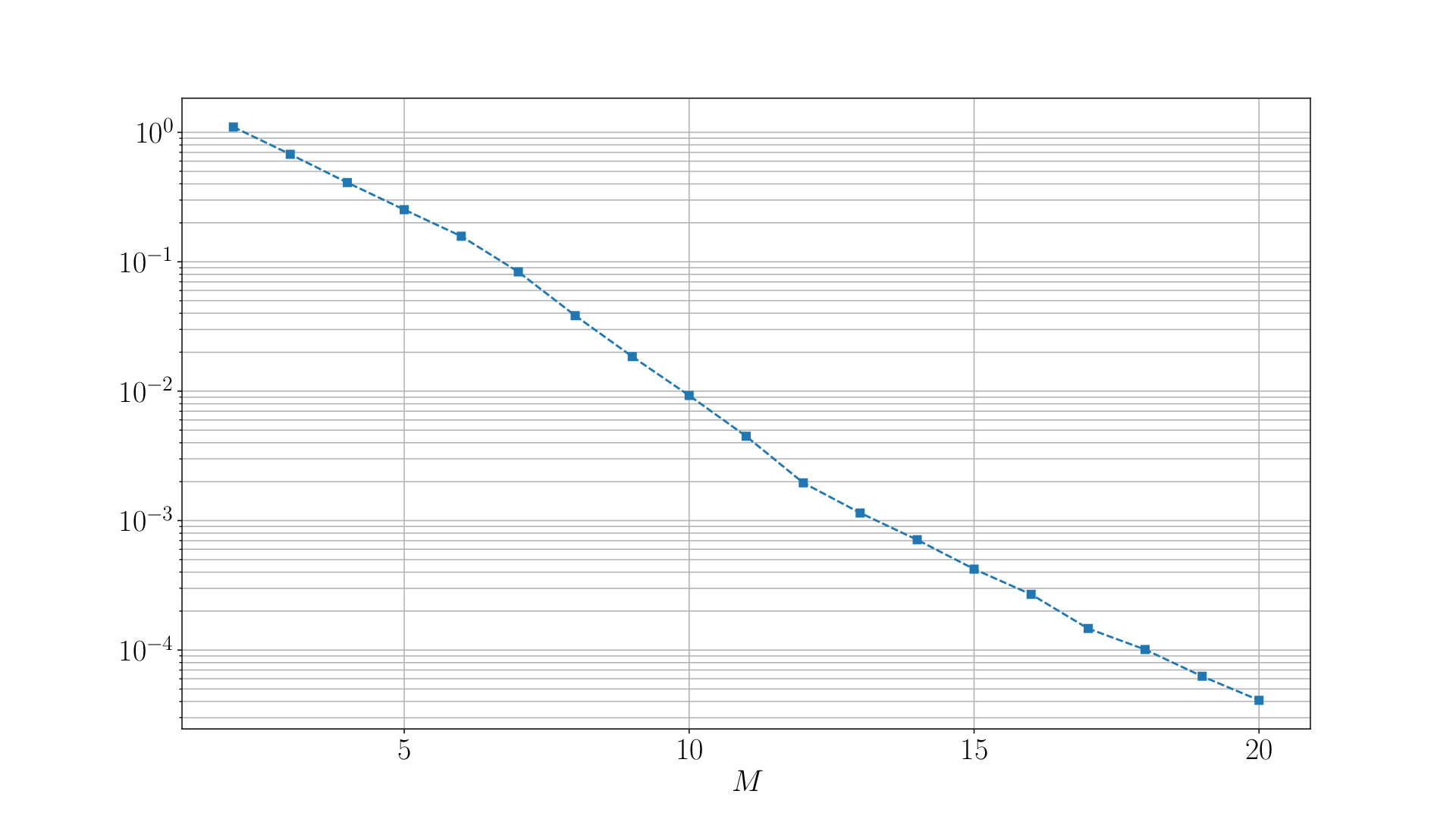
Refer to caption
Figure 7. Relative H1H^{1}-error ‖ulod,kn−ulod,kn,rb‖H1/‖ulod,kn‖H1\|u_{\mathrm{lod},k}^{n}-u^{n,\mathrm{rb}}_{\mathrm{lod},k}\|_{H^{1}}/\|u_{\mathrm{lod},k}^{n}\|_{H^{1}} between the solution with and without the reduced basis approach, plotted against the number of pre-computed solutions.

References

  • [1] A. Abdulle and P. Henning. Localized orthogonal decomposition method for the wave equation with a continuum of scales. Math. Comput., 86(304):549–587, 2017.
  • [2] G. Avalos and I. Lasiecka. Optimal blowup rates for the minimal energy null control of the strongly damped abstract wave equation. Ann. Sc. Norm. Super. Pisa Cl. Sci. (5), 2(3):601–616, 2003.
  • [3] J. Azevedo, C. Cuevas, and H. Soto. Qualitative theory for strongly damped wave equations. Mathematical Methods in the Applied Sciences, 40, 08 2017.
  • [4] I. Babuska and J. E. Osborn. Generalized finite element methods: Their performance and their relation to mixed methods. Siam Journal on Numerical Analysis - SIAM J NUMER ANAL, 20:510–536, 06 1983.
  • [5] I. Babuska and R. Lipton. Optimal local approximation spaces for generalized finite element methods with application to multiscale problems. SIAM Journal on Multiscale Modeling and Simulation, 9, 04 2010.
  • [6] E. Bonetti, E. Rocca, R. Scala, and G. Schimperna. On the strongly damped wave equation with constraint. Communications in Partial Differential Equations, 42(7):1042–1064, 2017.
  • [7] A. Carvalho and J. Cholewa. Local well posedness for strongly damped wave equations with critical nonlinearities. Bulletin of The Australian Mathematical Society - BULL AUST MATH SOC, 66, 12 2002.
  • [8] C. Cuevas, C. Lizama, and H. Soto. Asymptotic periodicity for strongly damped wave equations. Abstract and Applied Analysis, 2013, 09 2013.
  • [9] N. Dal Santo, S. Deparis, A. Manzoni, and A. Quarteroni. Multi space reduced basis preconditioners for large-scale parametrized PDEs. SIAM J. Sci. Comput., 40(2):A954–A983, 2018.
  • [10] M. Drohmann, B. Haasdonk, and M. Ohlberger. Adaptive reduced basis methods for nonlinear convection-diffusion equations. In Finite volumes for complex applications VI. Problems & perspectives. Volume 1, 2, volume 4 of Springer Proc. Math., pages 369–377. Springer, Heidelberg, 2011.
  • [11] C. Engwer, P. Henning, A. Målqvist, and D. Peterseim. Efficient implementation of the localized orthogonal decomposition method. Computer Methods in Applied Mechanics and Engineering, 350:123–153, 06 2019.
  • [12] F. Gazzola and M. Squassina. Global solutions and finite time blow up for damped semilinear wave equations. Ann. Inst. H. Poincaré Anal. Non Linéaire, 23(2):185–207, 2006.
  • [13] P. J. Graber and J. L. Shomberg. Attractors for strongly damped wave equations with nonlinear hyperbolic dynamic boundary conditions. Nonlinearity, 29(4):1171, 2016.
  • [14] B. Haasdonk, M. Ohlberger, and G. Rozza. A reduced basis method for evolution schemes with parameter-dependent explicit operators. Electron. Trans. Numer. Anal., 32:145–161, 2008.
  • [15] P. Henning and A. Målqvist. Localized orthogonal decomposition techniques for boundary value problems. SIAM Journal on Scientific Computing, 36(4):A1609–A1634, 2014.
  • [16] P. Henning, A. Målqvist, and D. Peterseim. A localized orthogonal decomposition method for semi-linear elliptic problems. ESAIM: Mathematical Modelling and Numerical Analysis - Modélisation Mathématique et Analyse Numérique, 48(5):1331–1349, 2014.
  • [17] T. J. Hughes, G. R. Feijóo, L. Mazzei, and J.-B. Quincy. The variational multiscale method—a paradigm for computational mechanics. Computer methods in applied mechanics and engineering, 166(1-2):3–24, 1998.
  • [18] R. Ikehata. Decay estimates of solutions for the wave equations with strong damping terms in unbounded domains. Mathematical Methods in the Applied Sciences, 24:659 – 670, 06 2001.
  • [19] T. J.R. Hughes, G. R. Feijóo, L. Mazzei, and J.-B. Quincy. The variational multiscale method - a paradigm for computational mechanics. Computer Methods in Applied Mechanics and Engineering, 166:3–24, 11 1998.
  • [20] V. Kalantarov and S. Zelik. A note on a strongly damped wave equation with fast growing nonlinearities. Journal of Mathematical Physics, 01 2015.
  • [21] P. Kelly. Solid Mechanics Part I: An Introduction to Solid Mechanics. University of Auckland, 2019.
  • [22] A. Khanmamedov. Strongly damped wave equation with exponential nonlinearities. Journal of Mathematical Analysis and Applications, 419(2):663 – 687, 2014.
  • [23] M. Larson and A. Målqvist. Adaptive variational multiscale methods based on a posteriori error estimation: Energy norm estimates for elliptic problems. Computer Methods in Applied Mechanics and Engineering, 196:2313–2324, 04 2007.
  • [24] S. Larsson, V. Thomée, and L. B. Wahlbin. Finite-element methods for a strongly damped wave equation. IMA Journal of Numerical Analysis, 11(1):115–142, 1991.
  • [25] Y. Lin, V. Thomée, and L. Wahlbin. Ritz-Volterra projections to finite element spaces and applications to integro-differential and related equations. Technical report (Cornell University. Mathematical Sciences Institute). Mathematical Sciences Institute, Cornell University, 1989.
  • [26] A. Målqvist and D. Peterseim. Generalized finite element methods for quadratic eigenvalue problems. ESAIM Math. Model. Numer. Anal., 51(1):147–163, 2017.
  • [27] A. Målqvist and D. Peterseim. Numerical Homogenization beyond Periodicity and Scale Separation. to appear in SIAM Spotlight, 2020.
  • [28] A. Målqvist and A. Persson. Multiscale techniques for parabolic equations. Numerische Mathematik, 138(1):191–217, 2018.
  • [29] A. Målqvist and D. Peterseim. Computation of eigenvalues by numerical upscaling. Numerische Mathematik, 130, 12 2012.
  • [30] A. Målqvist and D. Peterseim. Localization of elliptic multiscale problems. Math. Comp., 83(290):2583–2603, 2014.
  • [31] P. Massatt. Limiting behavior of strongly damped nonlinear wave equations. Journal of Differential Equations, 48:334–349, 06 1983.
  • [32] D. Peterseim. Variational multiscale stabilization and the exponential decay of fine-scale correctors. In Building bridges: connections and challenges in modern approaches to numerical partial differential equations, volume 114 of Lect. Notes Comput. Sci. Eng., pages 341–367. Springer, [Cham], 2016.
  • [33] A. Quarteroni, A. Manzoni, and F. Negri. Reduced basis methods for partial differential equations. an introduction. 2016.
  • [34] V. Thomée. Galerkin Finite Element Methods for Parabolic Problems. Springer Series in Computational Mathematics. Springer-Verlag, Berlin, second edition, 2006.
  • [35] G. F. Webb. Existence and asymptotic behavior for a strongly damped nonlinear wave equation. Canadian Journal of Mathematics, 32(3):631–643, 1980.