Constantin Christof
On the Stability Properties and the Optimization Landscape of Training Problems with Squared Loss for Neural Networks and General Nonlinear Conic Approximation Schemes
Abstract
We study the optimization landscape and the stability properties of training problems with squared loss for neural networks and general nonlinear conic approximation schemes in a deterministic setting. It is demonstrated that, if a nonlinear conic approximation scheme is considered that is (in an appropriately defined sense) more expressive than a classical linear approximation approach and if there exist unrealizable label vectors, then a training problem with squared loss is necessarily unstable in the sense that its solution set depends discontinuously on the label vector in the training data. We further prove that the same effects that are responsible for these instability properties are also the reason for the emergence of saddle points and spurious local minima, which may be arbitrarily far away from global solutions, and that neither the instability of the training problem nor the existence of spurious local minima can, in general, be overcome by adding a regularization term to the objective function that penalizes the size of the parameters in the approximation scheme. The latter results are shown to be true regardless of whether the assumption of realizability is satisfied or not. It is further established that there exists a direct and quantifiable relationship between the analyzed instability properties and the expressiveness of the considered approximation instrument and that the set of training label vectors and, in the regularized case, Tikhonov regularization parameters that give rise to spurious local minima has a nonempty interior. We demonstrate that our analysis in particular applies to training problems for free-knot interpolation schemes and deep and shallow neural networks with variable widths that involve an arbitrary mixture of various activation functions (e.g., binary, sigmoid, tanh, arctan, soft-sign, ISRU, soft-clip, SQNL, ReLU, leaky ReLU, soft-plus, bent identity, SILU, ISRLU, and ELU). In summary, the findings of this paper illustrate that the improved approximation properties of neural networks and general nonlinear conic approximation instruments come at a price and are linked in a direct and quantifiable way to undesirable properties of the optimization problems that have to be solved in order to train them.
keywords
loss surface, optimization landscape, stability properties, squared loss, neural networks, sensitivity analysis, nonlinear approximation, spurious local minima1 Introduction
The aim of this paper is to study the stability properties and the optimization landscape of training problems of the form
| (1) |
Here, is supposed to be a nonempty set (the set of input elements), is supposed to be a finite-dimensional vector space over that is endowed with an inner product and the associated norm (the output space), , , is assumed to be an arbitrary but fixed approximation scheme (e.g., a neural network) that can be adjusted by selecting an -dimensional vector from a nonempty set of admissible parameters (these may be weights, biases, coefficients, or something else), and , , , , is a given training set consisting of a label vector and an input vector . Note that, by introducing the abbreviations
| (2) |
the problem (1) can also be written in the more compact form
| (3) |
We prove that, if is more expressive than a linear approximation instrument, if the set is a cone, and if the number of samples is so large that there exist training label vectors for which the optimal value of (1) is positive (i.e., that are not realizable), then the problem (1) always suffers from spurious local minima/spurious basins, saddle points, instability effects, and/or the nonuniqueness of solutions for certain choices of the label vector . This illustrates that undesirable properties of the minimization problem (1) always appear if is trained in a not sufficiently overparameterized regime. We moreover show that, in the presence of label vectors with a positive optimal loss value and under appropriate assumptions on , there is a direct and quantifiable relationship between the instability properties of (1), the size of the set of vectors for which spurious local minima/spurious basins exist, and the approximation power of . This establishes a quid-pro-quo relationship between the expressiveness of and undesirable properties of (1). Compare also with the illustrative example in Section 4 in this context.
For problems (1) for which the optimal value of the loss function is identical zero for all , we establish that non-optimal stationary points, spurious local minima, and instability effects may still occur if a local linear/quadratic approximation of is not able to fit arbitrary with zero error. We moreover prove that the same is true for training problems that include an additional regularization term in the objective function. This shows that, although problems concerning spurious local minima, saddle points, and instability properties may be mitigated by overparameterization and classical Tikhonov regularization, one cannot expect that such techniques resolve these undesirable effects entirely. For an overview of the various theorems on the properties of squared-loss training problems for general approximation schemes proved in this paper, see Section 2.2.
A main feature of our analysis is that it is axiomatic and discusses the properties of training problems of the form (1) on a general level. Because of this, our results are not restricted to a certain type of approximation instrument but can readily be applied to all functions that satisfy the required abstract assumptions. This offers the additional benefit of giving an insight into the mathematical mechanisms that are behind, e.g., the emergence of spurious local minima in training problems of the form (1) and also allows to unify various previous results on the topic. For an overview of the consequences that our analysis has for neural networks, we refer to Section 2.3 below. Moreover, our approach also allows to establish new results on the properties of squared-loss training problems. In contrast to prior contributions, we are, for example, able to rigorously prove that a training problem of the form (1) satisfying mild assumptions always possesses spurious local minima for all label vectors in a nonempty open cone when is a deep neural network that involves activation functions which are affine on an open nonempty interval, see Corollaries 47 and 48. Further, we can establish that these spurious minima can be arbitrarily bad in relative and absolute terms and in terms of loss. For a detailed discussion of this topic, see Sections 2.3 and 2.4 below. In summary, this paper thus provides an in-depth analysis of what can and—maybe more importantly—what cannot be expected regarding the presence of spurious local minima and instability effects when studying squared-loss training problems of the form (1) for nonlinear approximation schemes in different training regimes.
We conclude this introduction with a brief summary of the content and the structure of the remainder of the paper:
In Section 2, we give an overview of our main theorems and the consequences that our analysis has for neural networks. Here, we also discuss in more detail the contribution of the paper and relations to previous work. Section 3 is concerned with preliminaries and basic concepts that are needed for the rigorous analysis of the training problem (1). In Section 4, we discuss a toy example that illustrates the basic ideas of our approach and provides some intuition on how the approximation properties of a function are related to the loss landscape of training problems of the form (1). The subsequent Section 5 contains the bulk of our analysis of the optimization landscape and the stability properties of training problems with squared loss for general approximation schemes. Here, we rigorously prove the main results presented in Section 2. Section 6 addresses the consequences that the analysis of Section 5 has for special instances of nonlinear conic approximation instruments, namely, classical free-knot interpolation schemes and deep and shallow neural networks. This section in particular includes the rigorous proofs of the results collected in Section 2.3. In Section 7, we conclude the paper with additional remarks on the overall role that our results play in the study of neural networks and the field of approximation theory.
2 Overview of Main Theorems and Discussion of Contribution
In this section, we discuss the background of our work and summarize our contributions.
2.1 Background
Due to the widespread use of the quadratic loss function, minimization problems of the type (1) (or (3), respectively) are encountered very frequently in machine learning and the field of approximation theory in general. One of the main reasons why problems of the form (1) are considered so often in the literature is that solving them (or, at least, solving them approximately) by means of classical first-order methods works very well in practical applications—in particular in the context of neural networks. This has led some authors to speculate that training problems of the type (1) are always very well behaved when neural networks are considered, e.g., in the sense that all local minima of (1) are also globally optimal or achieve a loss that is very close to the optimum. Compare, for instance, with the numerical results and conclusions of LeCun et al. 2015, Nguyen et al. 2018, and Yu and Chen 1995 in this context. At least for neural networks with linear activation functions, the belief that problems of the form (1) always possess very nice properties turns out to be not completely unfounded. Indeed, Kawaguchi 2016 could prove that, for deep linear neural networks, local minima of (1) are always also globally optimal so that—as far as the notion of local optimality is concerned—(1) effectively behaves like a convex problem. This effect was later also discussed in more detail by Zhou and Liang 2017, Laurent and von Brecht 2018, and Yun et al. 2019, and, with view on the convergence properties of gradient descent algorithms, by Eftekhari 2020 and Zou et al. 2020.
Unfortunately, for truly nonlinear approximation schemes,
the picture turns out to be more bleak.
Although there have been numerous attempts
to establish, for instance, the “local minima = global minima”-property
for networks with nonlinear activation functions (Eftekhari 2020; Saxe et al. 2014, mostly based on the
hope that the linear case gives a good enough impression of the nonlinear one,
see), the results that have been obtained in this context so far
are typically only applicable in very special situations and under rather restrictive assumptions
on the network architecture, the degree of overparameterization, and/or the
considered training data.
Compare, for instance, with the findings of
Yu and Chen 1995; Kazemipour et al. 2020; Li and Liang 2018; Li et al. 2021; Liang et al. 2018; Oymak and Soltanolkotabi 2020; Soudry and Carmon 2016; Cooper 2020 in this regard.
For a critical discussion of this topic and further references, see also Goldblum et al. 2020
and Ding et al. 2020.
The reason behind these deficits of the known positive results
on the loss surface of general neural networks is that even
slightest nonlinearities in the activation function can have a huge impact on the
optimization landscape of training problems of the form (1)
and may very well give rise to
spurious (i.e., not globally optimal) local minima. Data sets illustrating this for
two-layer ReLU neural networks have been constructed, for example, by
Swirszcz et al. 2016, Zhou and Liang 2017, and Safran and Shamir 2018. The minima documented in
the latter of these papers
have recently also been studied in more detail by Arjevani and Field 2021.
Further, Yun et al. 2019 showed that for two-layer ReLU-like networks spurious local minima
emerge for almost all choices of the training data.
This illustrates that local minima that are not globally optimal are not the exception but rather the rule
when piecewise linear activation functions are considered.
Yun et al. 2019 also provide
explicit examples of training problems for non-ReLU neural networks with two layers
which possess non-globally optimal local minima.
For problems involving only a single neuron,
an example with numerous local minima can also be found in
the early work of Auer et al. 1996.
Compare also with the results on spurious valleys of
Nguyen et al. 2018; Venturi et al. 2019 in this context,
and, for an overview of papers on the existence of spurious local minima, with Sun 2019; Sun et al. 2020.
What all of the results on the existence of spurious local minima in the above contributions have in common is that
they are only concerned with networks which are rather shallow (with depth not exceeding two).
The reason for this is that, as soon as more layers are considered,
the explicit construction of (nontrivial) spurious local minima—or, more precisely, proving that a constructed
local minimum is indeed not a global one—becomes
very cumbersome.
Two of the few contributions that address the construction of
spurious local minima for networks of arbitrary depth are
the recent ones of Goldblum et al. 2020 and Ding et al. 2020.
In both of these papers, however, a detailed discussion of the neuralgic point of
whether the constructed local minima are really spurious
is largely avoided. Goldblum et al. 2020 address this issue merely by providing
numerical evidence, and Ding et al. 2020 resort to the assumption of realizability
to resolve this problem11
1
While this was correct at the time of writing,
in a revised version of their paper,
Ding et al. 2020 were able to lift the assumption of realizability
for a certain class of spurious local minima constructed for -activations,
see (Ding et al. 2020, Theorem 1). The technique used to accomplish this,
however, does not carry over to activations with an affine segment, see
(Ding et al. 2020, Theorem 2, Corollary 1).
Our Corollaries 47 and 48 are able to fill this gap, cf. the discussion in Section 2.4 below.
.
What is further noteworthy is that the majority of
contributions on the existence of spurious local minima
currently found in the literature rely on the fact that neural networks
with piecewise linear activation functions are able to locally emulate a linear
neural network and thus inherit the solutions of training problems of the form
(3) for linear approximation schemes as spurious local minima.
Compare, for instance, with the methods of proof used by
Yun et al. 2019; Goldblum et al. 2020; Ding et al. 2020 in this context.
2.2 Overview of Main Theorems on General Approximation Schemes
The purpose of the present paper is to demonstrate that the undesirable properties of the optimization landscape of training problems of the form (3) for neural networks with nonlinear activation functions are, in fact, not the result of a particular choice of network architecture but rather a necessary consequence of the improved approximation properties that neural networks enjoy in comparison with linear approaches. More precisely, in what follows, we will demonstrate that indeed every nonlinear approximation scheme that is conic and—in an appropriate sense—more expressive than a linear approximation instrument (regardless of whether it is a neural network or something different, e.g., an adaptive interpolation approach) gives rise to squared-loss training problems that suffer from stability and uniqueness issues and/or the existence of non-optimal stationary points.
The starting point of our analysis is the observation that the overwhelming majority of nonlinear approximation schemes currently found in the literature possess the following two properties for all and all training data vectors with for all :
- I)
(Conicity) The set (with etc. defined as in Equation 2) is a cone, i.e.,
- II)
(Improved Expressiveness) The map satisfies
Note that the first of the above conditions is rather unremarkable. If, for example, a neural network is considered, then this assumption is automatically satisfied since the topmost layer is affine, see Lemma 36. Property II) is more interesting in this context. It expresses that, for the considered data vector , the function is able to provide an approximation of every nonzero training label vector that is better than the trivial guess . The main point here is that the map can accomplish this regardless of the relationship between the number of parameters and the number of training samples (and in particular also in those situations with ). For further details on this topic, we refer to Section 4.
For every training problem of the type (3) that involves an approximation scheme and a training data vector satisfying I) and II), we are able to prove the following (see the theorems in brackets for the mathematically rigorous statements):
- •
(Nonuniqueness and Instability of Best Approximations) If there exist label vectors that are not realizable, then the map is always unable to provide unique best approximations for all . (See Definition 3 for the precise definition of what we mean with the term “best approximation” here.) Further, arbitrarily small perturbations in can cause arbitrarily large changes in the set of best approximations. The degree of discontinuity of the best approximation map depends on the extent to which and satisfy condition II). (See Theorem 15.)
- •
(Choice Between Excessive Nonuniqueness and Spurious Minima/Basins) If there exist label vectors that are not realizable and if the map is continuous, then there exist uncountably many label vectors for which provides infinitely many best approximations or there exists an open nonempty cone such that, for each , (3) possesses spurious local minima and/or spurious basins. (See Theorem 17.)
- •
(Existence of Undesirable Stationary Points) If the map is differentiable at a point and if the function value and partial derivatives of at do not span the whole of , then there exist uncountably many such that is an arbitrarily bad saddle point or spurious local minimum of (3). In particular, in the case , every point of differentiability of is a saddle or spurious local minimum of (3) for uncountably many . The position of these depends on the extent to which and satisfy II). (See Theorem 19.)
- •
(Existence of Spurious Local Minima) If is able to locally parameterize a proper subspace of , then there exists an open nonempty cone such that (3) possesses spurious local minima for all . These spurious minima satisfy a growth condition in and can be arbitrarily bad in relative and absolute terms and in terms of loss. The size of depends on the extent to which and satisfy II). If every vector is realizable, then it holds . (See Theorem 22.)
- •
(Instability and Nonuniqueness in the Presence of Realizability) If there exists an such that maps an open neighborhood of into a proper subspace of and if every is realizable, then the solution set of (3) is instable w.r.t. perturbations of the vector and (3) is not uniquely solvable (in the sense of minimizing sequences) for certain choices of the vector . (See Corollary 23.)
- •
(Ineffectiveness of Regularization) If a term of the form with a and a regularizer is added to the objective function of (3), then the following is true (under appropriate assumptions on and , see Section 5.3):
- i)
There exists an open nonempty set such that, for all label vectors and regularization parameters with , the regularized training problem possesses a spurious local minimum. Further, these spurious minima can be arbitrarily bad in terms of loss. (See Theorem 27 and Remark 28.)
- ii)
There exist uncountably many combinations of and such that the resulting regularized training problem is not uniquely solvable (in the sense of minimizing sequences) and possesses a discontinuous solution map. (See Theorem 30.)
- iii)
Regardless of the choice of , adding the term to the objective function of (3) compromises the approximation property II). (See Theorem 29.)
- i)
Before we comment in more detail on how the above results are related to the literature and on the overall contribution of this paper, we briefly summarize the consequences that our analysis has for the study of neural networks.
2.3 Overview of Main Consequences for Deep and Shallow Neural Networks
Our first main result on neural networks establishes that these special instances of nonlinear approximation schemes are indeed covered by our abstract analysis:
- •
(Conicity and Improved Expressiveness of Neural Networks) Consider a fully connected feedforward neural network with input space , output space , , depth , widths , and activation functions , . Suppose that an with and an satisfying for all is given, and that one of the following is true:
- i)
The functions are of Heaviside type for all and it holds .
- ii)
The set can be decomposed into two (possibly empty) disjoint index sets and such that the function is of “sigmoid type” (e.g., sigmoid, tanh, arctan, soft-sign) for all , such that the function is of “ReLU type” (e.g., ReLU, soft-plus, swish) for all , such that holds for all , and such that holds in the case and in the case .
Then, the neural network and satisfy I) and II). (See Lemma 38 and Theorem 39.)
- i)
We remark that the fact that neural networks indeed possess property II) under the above weak assumptions on the data, the network architecture, and the activation functions is also interesting on its own. (See 35 for our precise assumptions and Lemmas 38 and 39 for an explanation of what we mean with the terms “sigmoid type”, “ReLU type”, and “Heaviside type” here.) We will comment in more detail on this topic in Section 2.4. For a result that shows that our analysis also covers ResNets, we refer the reader to Corollary 52. Given a training problem of the type (3) for a neural network and a vector that satisfy the conditions in the last bullet point, we obtain, for instance, the following corollaries from our abstract analysis (see again the results in brackets for the mathematically rigorous statements):
- •
(Nonuniqueness and Instability of Best Approximations) If there exist unrealizable label vectors , then the neural network is unable to provide unique best approximations for all . Further, arbitrarily small perturbations of the label vector can affect the set of best approximations to an arbitrarily large extent. The degree of discontinuity of the best approximation map depends on the extent to which and the considered network satisfy II). (See Corollary 43.)
- •
(Choice Between Excessive Nonuniqueness and Spurious Minima/Basins) If there exist unrealizable label vectors and if the activation functions , , are continuous, then there exist uncountably many for which the neural network provides infinitely many best approximations or there exists an open nonempty cone such that, for each , the training problem (3) possesses (arbitrarily bad) spurious local minima and/or spurious basins. (See Corollary 44.)
- •
(Saddle Points and Spurious Minima in the Non-Overparameterized Case) If the number of parameters in the neural network is smaller than the product , then every point of differentiability of the neural network is a saddle point or a spurious local minimum of (3) for uncountably many and, as a saddle point or spurious local minimum, can be made arbitrarily bad in relative and absolute terms and in terms of loss by choosing appropriately. The position of these depends on the extent to which and the considered network satisfy II). (See Corollary 45.)
- •
(Saddle Points and Spurious Minima for Arbitrary Problems) If holds and if the functions are differentiable, then there exists an -dimensional subspace of the parameter space of the network such that each element of this subspace is a saddle point or a spurious local minimum of (3) for uncountably many . Again, these points can be made arbitrarily bad in relative and absolute terms and in terms of loss by choosing appropriate . (See Corollary 46.)
- •
(Spurious Local Minima for Activation Functions with an Affine Segment) If each is affine-linear on some open nonempty interval of its domain of definition and if it holds and , then there exists an open, nonempty cone such that (3) possesses a spurious local minimum for each . The size of this cone depends on the extent to which and the neural network satisfy II). If every vector is realizable, then the cone is dense in and the solution map of (3) is discontinuous. Further, by choosing appropriate , the spurious local minima can be made arbitrarily bad in relative and absolute terms and in terms of loss. (See Corollaries 47, 48 and 50.)
- •
(Ineffectiveness of Regularization for Differentiable Activation Functions) If the activation functions are twice differentiable, if holds, and if the training problem (3) is regularized by adding a term of the form , , , to the objective function, where denotes the -norm on the Euclidean space, then there exists an open nonempty set such that the resulting regularized training problem possesses an (arbitrarily bad) spurious local minimum for all and there exist uncountably many values of such that the regularized training problem is not uniquely solvable and possesses a discontinuous solution map. (See Corollary 51.)
Note that the set-valuedness and the instability of the best approximation map in points one and two above immediately carry over to the solution operator of the problem (3) w.r.t. (just by taking preimages under the function ). For details on this topic, see the comments after Lemma 4 and Remark 16. We further would like to stress that the nonuniqueness of best approximations in, e.g., Corollary 43 has nothing to do with symmetries in the parameterization of a neural network. On the contrary, it expresses that there are different choices of the biases and weights (or, at least, minimizing sequences) which yield the same optimal loss in (3) but give rise to functions that act differently not only on unseen data but even on the training data set (see Remark 16 for more details). Regarding Corollaries 45 and 46, we would like to point out that the fact that the saddle points and spurious local minima of (3) can be made arbitrarily bad is not merely a consequence of the conicity property I). Indeed, it is easy to check that simply scaling the involved vectors cannot affect how well a non-optimal point performs in relative terms, cf. Remark 20. Lastly, we would like to emphasize that our abstract analysis is not only applicable to deep and shallow neural networks but also to other nonlinear conic approximation instruments. For an example demonstrating this, we refer the reader to Section 6.1 where our results are applied to a free-knot spline interpolation scheme that has also been considered by Daubechies et al. 2019 and can be interpreted as a classical nonlinear dictionary approximation approach (DeVore 1998, cf.). We only summarize the consequences of our abstract analysis for neural networks in this subsection because we expect that this is what the majority of readers are interested in.
2.4 Contribution of the Paper and Comparison with Known Results
The main contribution of this paper is that it establishes a direct and quantifiable connection between the improved approximation properties that nonlinear approximation schemes like neural networks enjoy over their linear counterparts and undesirable properties of the optimization problems that have to be solved in order to train a nonlinear approximation instrument on a given data set. Compare, for instance, with the estimates (27), (38), and (43) in this context, which show that the degree of discontinuity of the best approximation map of a given nonlinear conic approximation scheme , the position of the label vectors that cause a given point to be a saddle point or a spurious local minimum in Theorem 19, and the size of the cone of “bad” label vectors in Theorem 22 depend directly on the extent to which the considered approximation instrument satisfies condition II). At least to the best of the author’s knowledge, this relationship between the expressiveness of an approximation scheme and the loss landscape of the associated training problems has not been explored systematically so far in the literature (although it is, of course, closely related to classical topics of nonlinear approximation theory and the study of nonlinear least-squares problems). Note that the results of this paper can be interpreted as an instance of the well-known fact that there is “no free lunch” as they show that the improved approximation properties of, e.g., neural networks come at the price that the associated training problems are always potentially ill-posed in the sense of Hadamard and possess spurious local minima or saddle points for certain choices of the training data. For further details on this topic and its relationship to the curse of dimensionality and the problem of NP-hardness, see also Section 7.
We would like to emphasize that the connections that we draw in this paper are not only interesting for their own sake but also allow to improve and complement known results on the optimization landscape of training problems with squared loss found in the literature. By exploiting the approximation property II), for example, we are able to show that the assumption of realizability used in (Ding et al. 2020, Corollary 1) to establish that certain local minima are not globally optimal is unnecessary, that the conditions on the network widths in (Ding et al. 2020, Assumption 3) can be relaxed, and that the observations made in the numerical experiments of Goldblum et al. 2020 can also be backed up analytically, cf. Corollaries 44, 47 and 48. The main point in this context is that the approximation property II) allows to prove that a point is a spurious local minimum of a problem of the type (3) without the explicit construction of a parameter that yields a smaller loss than . This makes the rather cumbersome calculations that are normally used to establish that a local minimum is not globally optimal unnecessary, cf. the proofs of Theorems 19 and 21 and also the comments in the proof of (Yun et al. 2019, Theorem 1) where it is emphasized that constructing points with smaller function values is precisely the hard part of showing the existence of spurious local minima. We would like to point out that the difficulty of proving the spuriousness of a local minimum is also the reason why lifting the condition of realizability in (Ding et al. 2020, Corollary 1) is nontrivial. If realizability is assumed, then the optimal value of the loss function in (3) is known to be zero. Accordingly, in order to construct an example of a spurious local minimum, it suffices to construct a local minimum with a positive loss value. This can typically be done relatively easily by employing classical second-order sufficient conditions and by choosing the data of the problem appropriately. In the unrealizable setting, however, such a local construction is not sufficient anymore simply because it does not guarantee that the constructed local minimum is not a global one. To prove the latter, one needs global information about the neural network that cannot be obtained from derivative-based and, as a consequence, inherently local tools like second-order optimality conditions. With the property II), we are able to bridge this gap, see Corollaries 47 and 48. Since our approach does not require explicit constructions, we are also able to rigorously prove the existence of spurious local minima in situations in which the classical approach of manually checking the spuriousness of a local minimum becomes intractable due to the presence of additional regularization terms or the architecture of the considered nonlinear approximation scheme. Compare in particular with Corollaries 47, 48 and 51 in this context, which establish the existence of spurious local minima for both unregularized and regularized training problems and for neural networks with arbitrary depth and various activation functions. At least to the best of the author’s knowledge, results on the existence of spurious local minima with a comparable generality can currently not be found in the literature. In particular the existence of spurious local minima in Tikhonov-regularized problems for deep networks has apparently not been considered so far. Note that our approach additionally offers the advantage that it allows to establish that saddle points and spurious local minima of training problems with squared loss can be arbitrarily far away from global optima in relative and absolute terms and in terms of loss, see Lemmas 18, 19, 27 and 21 and the associated corollaries on neural networks in Section 6.
As already mentioned, by exploiting the approximation property II), we are also able to rigorously prove that solutions of training problems of the form (3) (or the associated best approximations, respectively) cannot be expected to be unique or stable with respect to perturbations of the training label vector , see Theorems 15, 30 and 23. This gives an analytic explanation for the instability effects that are commonly observed in network training, cf. Cunningham et al. 2000 and also the comments on the nonuniqueness of global solutions in (Cooper 2020, Section 1.1). We remark that, for neural networks with one hidden layer, instability results similar to that in our Theorem 15 have already been proved in the -spaces by Kainen et al. 1999; Kainen et al. 2001 by exploiting classical instruments of nonlinear approximation theory. The finite-dimensionality of the training problem (3) allows us to go further than the authors of these papers and to establish the nonuniqueness and instability of solutions and best approximations for neural networks of arbitrary depth. By exploiting the inequality of Jung (see Burago and Zalgaller 1988, Theorem 11.1.1), we are further able to establish a quantitative connection between the discontinuity properties of the best approximation map associated with (3) and the extent to which a function satisfies II), cf. (27). The results that we prove in this context also seem to be new.
We would like to point out that, for deep and shallow neural networks whose activation functions are affine-linear on some open nonempty interval of their domain of definition, our results give a quite complete picture of how the optimization landscape of problems of the form (3) depends on the approximation property II) or, more precisely, on the error bound defined in (15) that measures the extent to which property II) is satisfied. In the case (which corresponds to the situation where there are unrealizable label vectors), one has to deal with both the instability of the set of best approximations of (3) and the existence of an open nonempty cone of vectors for which (3) possesses (potentially arbitrarily bad) spurious local minima (see Corollaries 47, 48 and 43). The closer gets to zero (i.e., the more expressive the network becomes relative to , e.g., due to an increased number of network parameters or a smaller number of training pairs), the less pronounced the instability properties of the best approximation map of (3) are, see (27), and the larger the cone grows, see (43). Finally, in the case (i.e., the case where every vector is realizable, cf. Definition 8), the instability properties of the best approximation map are not present anymore and the cone is dense in so that, for almost all , (3) possesses spurious local minima. In summary, the above shows that, when considering problems of the type (3) for a network satisfying the assumptions of Corollary 47 or Corollary 48 or, more generally, a nonlinear conic approximation instrument satisfying the conditions in Theorem 22, one can never get rid of both the discontinuity of the best approximation map and spurious local minima. The problem (3) always possesses at least one property that is undesirable (cf. also with Theorem 17 in this context). Note that the fact that the instability properties of the best approximation map associated with (3) are not present when every vector is realizable provides a possible explanation for the often made observation that overparameterization benefits the training of neural networks in practical applications. Compare, e.g., with the results of Chen et al. 2020; Cooper 2020; Li and Liang 2018; Oymak and Soltanolkotabi 2020; Allen-Zhu et al. 2019; Soudry and Carmon 2016 in this context. However, it seems to be unlikely that this is the only reason for the advantageous properties that overparameterized training problems typically enjoy. In fact, one can see in Corollaries 23 and 30 that, even in the case where every vector is realizable and the objective contains additional regularization terms, there are still certain nonuniqueness and instability effects present in problems of the form (3). (These, however, are of a different quality than those arising from the nonuniqueness of best approximations in Theorem 15.) Note that the observation that neither by overparameterization nor by adding regularization terms to the objective function it is possible to completely remove the ill-posedness of training problems of the type (3) is also remarkable on its own.
Regarding the application of our abstract analysis to neural networks, we would like to stress that the fact that these special instances of nonlinear approximation schemes indeed satisfy the condition II) under the weak assumptions of Lemmas 38 and 39 is also interesting independently of the study of the loss landscape of training problems of the form (3). As we will see in Section 4, the property II) is a characteristic that distinguishes neural networks clearly from linear approximation schemes (e.g., polynomial approximation) and thus gives an idea of why these approximation instruments are able to outperform classical approaches. Compare also with Lemma 10 in this context which establishes that the property II) is directly related to worst-case estimates for the approximation error that nonlinear approximation schemes achieve for arbitrary training label vectors . We also would like to emphasize at this point that II) is a global property of an approximation scheme and thus of a completely different flavor than, e.g., the local properties of activation functions (for instance, piecewise linearity) that are commonly worked with in the analysis of neural networks. This also becomes apparent in the proof of Theorem 39 which, in contrast to many classical approaches, is not based on concepts like linearization but on the observation that the overwhelming majority of neural networks used in practice are able to emulate networks with binary activation functions by saturation and that the property II) is inherited from these binary networks obtained in the saturation limit. Further details on this topic can be found in Section 6.
We finally would like to emphasize that the theorems proved in this paper do not contradict the results on the absence of spurious local minima in training problems for neural networks with linear activation functions established, e.g., by Kawaguchi 2016; Zhou and Liang 2017; Laurent and von Brecht 2018. Since such networks give rise to functions that are affine and sets that are subspaces, they only satisfy condition II) in pathological situations and thus do not fall under the scope of, e.g., Theorems 17, 21 and 22. Compare again with the example in Section 4 in this context. Similarly, our theorems also do not contradict the results on the absence of spurious valleys established by Nguyen et al. 2018 and Venturi et al. 2019 (simply because we are mainly concerned with classical spurious local minima in this work, cf. Definition 5). They are, however, in good accordance with the observations on the role and presence of saddle points in network training made, e.g., by Dauphin et al. 2014. For further details on this topic and additional remarks on the relationship between our results and the literature, we refer the reader to the comments after the respective theorems in the subsequent sections.
3 Notation, Preliminaries, and Basic Concepts Needed for the Analysis
Before we begin with our analysis, we fix the notation and introduce some basic concepts. As already mentioned in the introduction, the main focus of this work will be on training problems of the form
| (4) |
For easy reference, we restate our assumptions on the quantities in (4) in:
Assumption 1 (Standing Assumptions and Notation).
- •
is a nonempty set,
- •
is a finite-dimensional vector space over that is endowed with an inner product and the associated norm (i.e., for all ),
- •
, , and is a nonempty set,
- •
is a function (representing an approximation scheme),
- •
, is the training data.
Note that the subscript is used in 1 to highlight that and take the role of the training data in (4) (in contrast to, e.g., the arbitrary elements of the space appearing in equation (8) below). We would like to point out that several of the results proved in the following sections can be extended (in one form or another) to more general loss functions and to infinite dimensions. See, for instance, (Christof and Hafemeyer 2021, Theorem 2.4) for an instability and nonuniqueness result for optimization problems in Banach spaces with an -loss structure that is similar in nature to Theorem 15 and also with the general theory of Chebychev sets found in (Braess 1986, Section II-3). We restrict the attention to the squared-loss function to be able to present the theory developed in this paper in a uniform manner and to make the proofs and discussion of results less cumbersome.
Next, we collect the abbreviations in (2).
Definition 2 (Some Abbreviations).
We remark that, here and in what follows, we always think of elements of the space as column vectors. As already pointed out in Section 1, the abbreviations in Definition 2 allow us to restate the problem (4) in the more compact form
| (6) |
Note that, since the objective function of (6) is not necessarily coercive w.r.t. , it can, in general, not be expected that (6) possesses a global minimizer . One can only guarantee that there exists a minimizing sequence , i.e., a sequence satisfying
| (7) |
as tends to infinity. (This is, for example, the case when some of the activation functions in a neural network have to saturate to fit a training vector precisely.) To get a grip on these effects, it makes sense to not only study local and global minimizers of (6) but also the set of all elements of that can be approximated by the function for a given and fit a training label vector in an optimal manner. This gives rise to:
Definition 3 (Best Approximation Map).
Let be arbitrary but fixed and let etc. be as before. Then, we define to be the map
| (8) |
Here, the symbol expresses that the function may be set-valued and with we denote the topological closure of a set in .
Note that the map is precisely the set-valued metric projection in onto the closure of the image of under the function for the given vector . Because of this, we in particular have:
Lemma 4 (Properties of the Set of Best Approximations).
Suppose that and are arbitrary but fixed. Then, the set is nonempty and compact for every training label vector .
Proof.
The nonemptyness and compactness of for all follow immediately from the fact that the minimization problem in the variable associated with the right-hand side of (8) possesses a nonempty, closed, and bounded set of solutions for all due to the continuity and coercivity of the norm, the closedness and nonemptyness of the set , the finite-dimensionality of , and the theorem of Weierstrass. ∎
We would like to point out that, by taking preimages and images under the function , properties of the map directly translate into properties of the optimization landscape of (6) and vice versa. If, for example, and are vectors such that holds for some and if we denote the closed balls in of radius around , , with , then, for every arbitrary but fixed with , we trivially have that the preimages
satisfy , , , and
The above implies that each of the two disjoint subsets and of the parameter space has to contain a global solution of the minimization problem (6) or a sequence satisfying (7). Note that the main advantage of considering the projection instead of the objective of (6) is that the former function allows to also detect those cases where (6) possesses spurious local minima “at infinity” in the sense that the optimization landscape of (6) possesses basins which stretch to the boundary of and do not contain a local minimum in the classical sense (so-called spurious basins). Compare, e.g., with the behavior of the function in this context and also with Theorem 17. Such cases should, of course, not be neglected as descent methods may very well get trapped in a non-optimal basin of this type and subsequently drive the parameter to the boundary of the set without approximating the optimal value of the loss function on the right-hand side of (7) in the limit. Completely analogously to the above, stability and instability properties of carry over to (6), too. For further details on this topic, we refer the reader to Remark 16.
For the sake of clarity, let us finally make precise what we mean with the terms “global minimum”, “local minimum”, “spurious local minimum”, etc. appearing in our analysis:
Definition 5 (Notions of Optimality).
Given a function that is defined on a subset of a normed space , we call a point a:
- •
global minimum (or, more precisely, global minimizer) of the function if holds for all .
- •
local minimum (or, more precisely, local minimizer) of the function if there exists a closed ball of radius in centered at such that holds for all .
- •
spurious local minimum of if is a local minimum but not a global minimum of .
- •
global (respectively, local, respectively, spurious local) maximum of if is a global (respectively, local, respectively, spurious local) minimum of the function .
- •
saddle point of if holds for some , is an element of the interior of , is differentiable at , it holds , and is neither a local minimum nor a local maximum of .
We remark that some authors apparently go so far as to call every point with a vanishing gradient and a vanishing Hessian a spurious local minimum. We believe that the term “spurious local minimum” should be reserved for points that are local minima. Finally, we would like to emphasize that, throughout this work, the symbols , , etc. always refer to the global notion of optimality (e.g., in the definition of the map ).
4 A Toy Problem Illustrating the Basic Ideas
Having introduced the necessary notation, we now turn our attention to the optimization landscape and the stability properties of training problems of the form (6). We begin with a simple example that illustrates the main ideas of our analysis and gives some intuition on why nonlinear approximation schemes may possess better approximation properties than their linear counterparts and on how these properties are related to the behavior of the function and the loss landscape of (6). To construct our example, let us suppose that
| (9) |
and that is an arbitrary but fixed training data vector which satisfies . Let us further assume, for a start, that we are given an approximation scheme , , that is linear in the sense that the function is linear in the parameter vector . Then, we trivially have
where denote the standard basis vectors of , and the training problem (6) can also be written as
| (10) |
for every arbitrary but fixed , where is the Euclidean norm on scaled with the factor and where , . For a linear scheme , (6) thus boils down to a standard approximation problem which aims to find a function in the linear subspace spanned by the set that fits the given function values at the locations optimally in the least-squares sense. Note that the structure of (10) in particular implies that, regardless of which linear scheme we consider here, there are always nontrivial choices of for which the problem (10) possesses the optimal solution so that does not provide an approximation of that is better than the trivial guess . Indeed, for all in the orthogonal complement of the space w.r.t. the Euclidean scalar product, we clearly have
Using the notation in Definition 2, this observation can also be expressed in the more compact form
| (11) |
For comparison, let us now consider the nonlinear approximation scheme
| (12) |
with given by
and define , , , by
Then, from the properties of , it follows straightforwardly that
holds for all with . This implies in particular that, for every arbitrary but fixed label vector , there exists a parameter such that the nonlinear approximation scheme (12) satisfies
namely, in the case , the vector with . In short,
| (13) |
The above result shows that the nonlinearity of the function in (12) indeed allows this map to possess better approximation properties than the linear schemes considered at the beginning of this section in the sense that, for every arbitrary but fixed nonzero , we can find an such that provides a loss that is smaller than that of the trivial guess and the associated vector . The map in (12) is thus able to approximate every given label vector at least to a small extent even in those situations where the problem (6) is grossly underparameterized, i.e., satisfies —a feature that is not obtainable with a scheme that is linear in and possesses the parameter space as we have seen in (11). Note that this property can also be interpreted as a “relaxed” version of realizability that holds for all label vectors regardless of the choice of and , cf. the analysis in Section 5.
However, the example (12) also immediately shows that the improved expressiveness in (13) does not come for free. If we consider, for instance, the image of the parameter space under the function associated with the nonlinear approximation scheme in (12) in the case for the training data vector , then it is readily seen that this set is a nontrivial union of numerous segments of two-dimensional subspaces, cf. Fig. 1. This implies in particular that the projection onto is not single-valued at all points and, as a consequence, that the best approximating element provided by is not uniquely determined for all possible choices of the training label vector . It is moreover easy to check that the locally affine-linear structure of the set entails that the optimization landscape of the training problem (6) for the approximation scheme in (12) possesses spurious local minima and saddle points for various choices of , cf. Propositions 21 and 22 below. The intuitive reason behind all these effects is that the same geometric properties of the image , that allow to satisfy (13), also imply that this set is folded in a way that causes the normal cones of various points on to intersect.
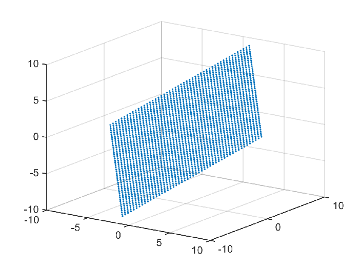
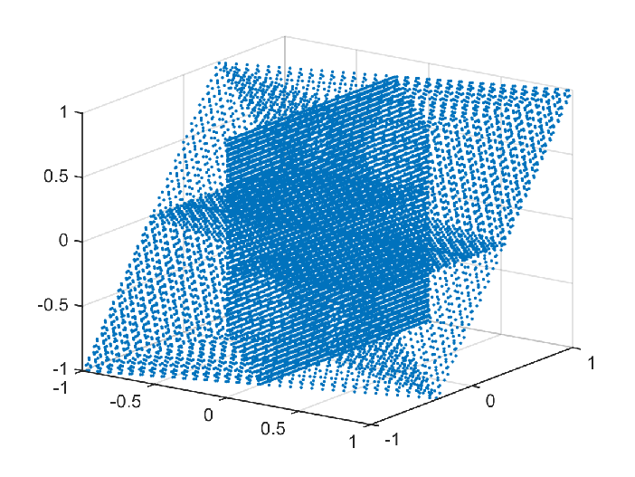
In the remainder of this paper, we will prove that the above undesirable properties of the function and the optimization problem (6) indeed inevitably appear when the considered approximation scheme satisfies (13) and is conic in the sense that the set is a cone. We will moreover demonstrate that nearly all commonly used nonlinear approximation instruments (and in particular neural networks) are covered by this setting and are thus subject to the above effects. Note that this also shows that (13) is, in fact, a quite fundamental property.
Before we demonstrate that the above observations indeed carry over to a far more general setting, we would like to point out that the example that we have studied in this section is a rather academic one. It is easy to check that the approximation scheme (12) possesses various properties that are highly undesirable and thus would never be a sensible choice for a practical application. Moreover, the scheme in (12) is clearly not conic and thus violates one of the main assumptions of the subsequent analysis. We remark that this second deficit can be fixed easily by adding a further parameter to , i.e., by considering the modified function , . In fact, after this modification, the resulting approximation instrument is nothing else than a simple neural network with a single neuron and a lightning-shaped activation function, cf. 35. We have considered the function in (12) in this section since, on the one hand, it possesses the property (13) and, on the other hand, satisfies for —thus enabling the visualization in Fig. 1. For the function , one has to consider at least samples to achieve that holds and for this dimension an illustration as in Fig. 1 is not possible anymore. (It seems to be difficult to construct an example of a function that satisfies both I) and II) and simultaneously for .) As already mentioned, we will see in Section 6 that various commonly used approximation schemes (and in particular general neural networks) exhibit a behavior that is very similar to that of the function in (12). In Section 5.2, we will moreover see that, at least as far as the existence of saddle points and spurious local minima is concerned, it is not essential that it holds as in the situation of (9).
5 Analysis and Rigorous Proofs in the Abstract Setting
The aim of this section is to study the behavior of the function and the loss landscape of the training problem (6) for a general, nonlinear, conic approximation scheme satisfying (13). Motivated by the observations made in Section 4 and by what is encountered in practical applications, we will consider the following setting:
Assumption 6.
(Standing Assumptions for the Analysis of Section 5) Let , , etc. be defined as in Section 3. We assume that an approximation scheme and an arbitrary but fixed training data vector are given such that the following two conditions are satisfied:
- I)
(Conicity) The set is a cone in the sense that
- II)
(Improved Expressiveness) The map satisfies
As already mentioned, various examples of approximation schemes satisfying the conditions in 6 will be presented in Section 6. Henceforth, the basic idea of our analysis will be to prove that the properties I) and II)—although very desirable from the approximation point of view—also automatically imply that training problems of the form (6) possess various disadvantageous properties. We begin with some basic observations:
Lemma 7 (Reformulation of the Improved Expressiveness Property).
Proof.
The implication “II) (14)” is trivial. To prove “(14) II)”, it suffices to note that, for every arbitrary but fixed , there exists a with
by Lemma 4 and to subsequently exploit the definition of the closure and the continuity of the norm . This also shows that it indeed makes sense to write “” on the left-hand side of (14) instead of “”. ∎
Note that Lemma 7 implies that II) is a property of the closure of the image of the map and completely independent of how this image is parameterized by the variable . To measure the extent to which condition II) is satisfied by a given approximation scheme, we introduce:
Definition 8 (Error Bound ).
In the situation of 6, we define
| (15) |
Remark 9.
The number is precisely the square of the deviation of the unit sphere in from the closure of the image of the map in the sense of nonlinear approximation theory, see (Kůrková and Sanguineti 2002, Section II). It corresponds to the squared worst-case approximation error achieved by the map w.r.t. the norm for label vectors chosen from the unit sphere in .
Using our assumptions I) and II) and the closedness of the set , it is easy to establish the following:
Lemma 10 (Properties of the Bound ).
Proof.
Using the distance function to the set w.r.t. the norm , the identity in (15) can also be written as
Since the map is continuous, since the unit sphere is compact due to the finite-dimensionality of , and since
| (18) |
holds for all by exactly the same arguments as in the proof of Lemma 7, it now follows immediately that there exists at least one with the properties in (17). Note that, in combination with II), this also yields
so that is an element of the interval as claimed. It remains to prove (16). To this end, we note that (18) and the cone property of the set , which follows immediately from I), imply that is an element of and that
holds for all . Combining the last two observations gives the desired estimate (16). This completes the proof. ∎
As Lemma 10 shows, the smaller the number , the better the ability of the function to fit arbitrarily chosen label vectors . However, since is also a measure for the nonlinearity of the considered approximation scheme (at least in the case ), one also has to expect that the optimization landscape of the problem (6) worsens as tends to zero, cf. the observations made in Section 4. In Section 5.2, we will see that such an effect is indeed present and that the value of also gives an estimate on how likely it is to encounter vectors for which the problem (6) possesses spurious local minima and saddle points, cf. Theorems 19 and 22.
Before we turn our attention to this topic, we study the:
5.1 Set-Valuedness and Discontinuity of the Best Approximation Map
Recall that we have defined to be the function that maps a label vector to the set of elements of the closure that attain the minimal loss in (6), i.e.,
The purpose of this subsection is to analyze which consequences the properties I) and II) in 6 have for this metric projection onto the set and the stability properties of the training problem (6). As talking about the map is only sensible when the closure of the image of is not the whole of (otherwise is just the identity map), throughout this subsection, we always assume the following:
Assumption 11.
(Existence of Unrealizable Vectors) It holds .
Note that 11 expresses that there exist label vectors that are unrealizable in the sense that they cannot be approximated by the function up to an arbitrary tolerance and thus yield a positive optimal value of the loss in (6). Such situations occur when optimization problems (6) are considered that are (roughly speaking) not sufficiently overparameterized, i.e., problems in which the number of training samples is too high relative to the approximation capabilities of the considered approximation instrument . Compare also with the comments after Corollary 44 in this context. We would like to emphasize that 11 is only needed for the analysis of this subsection and Theorem 17 in Section 5.2. For the derivation of our other results on stationary points and spurious local minima, it is sufficient to assume that a local approximation of the function is unable to fit arbitrary label vectors precisely, cf. Propositions 21, 22 and 23. The starting point for our study of the properties of the function is the following observation:
Lemma 12.
Proof.
Since holds and since the set is a closed cone, there exists at least one with and . This shows that the error bound has to be positive in the situation of the lemma and, in combination with Lemma 10, that holds as claimed. To prove the remaining assertions i), ii), and iii), let us assume that an arbitrary but fixed worst-case unit label vector as in (17) is given. (Recall that the existence of such a is guaranteed by Lemma 10.) Then, we obtain from Lemma 4 that the set contains at least one element and it follows from the second equality in (17), the fact that is smaller than one, and the definition of that has to hold. Since is a solution of the problem
and again due to the cone property of the set , we moreover have
| (20) |
Choosing parameters of the form with in (20), using the binomial identities, dividing by , and passing to the limit yields that has to hold and, as a consequence,
The above shows that is contained in the affine subspace in (19) and, since was an arbitrary element of , that . This establishes ii). To prove iii), we use a contradiction argument: Suppose that the vector is not an element of the convex hull . Then, by noting that the set is compact due to the finite-dimensionality of and the compactness of , see Lemma 4, and by applying the strong hyperplane separation theorem to the sets and , see (Rockafellar and Wets 1998, Theorem 2.39), we obtain that there exist a nonzero and constants and such that
holds for all and . Note that the above is only possible if and . We may thus conclude that , , and satisfy
| (21) |
Consider now for all sufficiently small the vectors and select arbitrary but fixed . (Recall that the sets are nonempty by Lemma 4.) Then, it follows from (16), the definition of , and the second property in (17) that , , and satisfy
| (22) |
Using the binomial identities, the properties and , and the definition of in (22) yields
Since the family is necessarily bounded (see the first inequality in Equation 22), the above implies that there exists a such that holds for all , where is the constant in (21), and, again by (21), that there exists an with for all . However, from the boundedness of and the closedness of the set , we also obtain that we can find a sequence with and for some , and, due to the convergence for and (22), such a clearly has to satisfy
The above yields and, as a consequence,
which is not possible. The vector thus has to be an element of the set and the proof of iii) is complete. Since the assertion in i) is a trivial consequence of ii), iii), and the fact that is smaller than one by Lemma 10, this concludes the proof of the lemma. ∎
Note that Lemma 12 implies that the cone can only be convex if it is equal to the whole space . By exploiting the properties I) and II) directly, we can also establish the following, stronger result on the geometry of this set:
Proposition 13 (Nonexistence of Solar Points).
Proof.
Consider an arbitrary but fixed and some . Then, it necessarily holds , and we obtain from the same arguments as in the proof of Lemma 12 that has to hold. Define and for all , and let be arbitrary but fixed elements of the sets for all . Then, from (16), the definition of , the orthogonality between and , and the equation , we obtain that
| (24) | ||||
holds for all . Since the set is dense in and since is an element of the interval by Lemma 12, the above shows that, for all with
we have
and, as a consequence, . This establishes the first claim of the proposition. The second one is an immediate consequence. ∎
It is easy to check that the property (23) implies that the set does not admit any supporting hyperplanes in the situation of Proposition 13. This shows that the cone indeed has to be highly nonconvex if the map satisfies I) and II) and there exist unrealizable vectors. Compare also with the geometry of the set in Fig. 1(b)) in this context. For further details on solar points and their role in the field of nonlinear approximation theory, we refer the reader to Braess 1986. We remark that arguments very similar to those in the proof of Proposition 13 will also be used in Section 5.2 for the derivation of our results on saddle points and spurious minima.
To study which consequences the inclusion in point iii) of Lemma 12 has for the continuity properties of the map , we need:
Lemma 14 (A Variant of Jung’s Inequality).
Suppose that is an affine-linear subspace of
with dimension . Assume further that a point , a
compact set , and a number satisfying
and for all
are given. Then, it is true that
| (25) |
Proof.
Note that, by introducing a suitably defined orthonormal basis and by restricting the attention to the space of directions of the affine subspace , we can always transform the situation considered in the lemma into that with and , where denotes the Euclidean norm. It thus suffices to prove (25) in the space for all , compact sets , and constants that satisfy and for all . So let us assume that such , , and are given, and suppose further that is a closed ball in with center and radius that covers the set . Then, in the case , our assumption for all immediately yields that has to hold. In what follows, we will show that this inequality is also true for . To this end, we note that the inclusion and Carathéodory’s theorem, see (Borwein and Vanderwerff 2010, Theorem 1.2.5), imply that there exist and satisfying and , and, as a consequence,
Here, denotes the Euclidean scalar product. The above implies in particular that there has to be at least one with , and from this inequality and the inclusion , it follows straightforwardly that
Thus, as claimed. In summary, we have now proved that every closed ball with has to have radius at least . In combination with the classical inequality of Jung, see (Burago and Zalgaller 1988, Theorem 11.1.1), this yields
Rearranging the above establishes (25) and completes the proof. ∎
By combining Lemmas 12 and 14 and by using elementary properties of the map , we now arrive at the following main result of this subsection:
Theorem 15.
(Nonuniqueness and Instability of Best Approximations) Suppose that 6 and 11 hold. Then, the best approximation map
associated with the training problem (6) has the following properties:
- i)
There are uncountably many such that contains more than one element.
- ii)
The function is discontinuous in the following sense: For every arbitrary but fixed , there exists an uncountable set such that, for every label vector , there exist sequences with
(26) Here, denotes the cardinality of a set and with we mean the distance between the elements of the singletons and . Further, for every , there exists at least one with the properties
(27)
Proof.
Let be an arbitrary but fixed worst-case unit label vector as in (17). Then, from Lemma 12, it follows that holds, and we obtain from the conicity of the set that satisfies for all and all . Combining these two observations yields for all which proves the assertion of i). To establish ii), we recall that, by Lemma 12, the compact set has to satisfy , where again denotes the affine subspace in (19), and that the definition of yields for all (see the first part of the proof of Lemma 12). The latter implies, in combination with the properties of , that
The vector and the number thus satisfy
and we may invoke Lemma 14 to deduce that there exist with
Consider now the sequence , . Then, we clearly have for and it holds
| (28) | ||||
with equality everywhere if and only if . In combination with the definition of , this implies in particular that holds for all . Completely analogously, we also obtain that the vectors , , satisfy for and for all . By again exploiting the positive homogeneity of the map and by combining all of the above, it now follows immediately that, for every arbitrary but fixed and all
we have
and
Since holds by (17), this establishes ii) and completes the proof. ∎
Several remarks are in order regarding the last result:
Remark 16.
- •
Theorem 15 shows that, if there exist label vectors that cannot be approximated up to arbitrary tolerances and if I) and II) hold, then the approximation scheme is always unable to provide unique best approximations for all possible choices of (see point one) and arbitrarily small perturbations in can change the set of best approximations to an arbitrarily large extent (see point two). This implies in particular that, in the situation of Theorem 15, the problem of finding best approximations for a given is always ill-posed in the sense of Hadamard for certain choices of .
- •
As already mentioned in the introduction, for neural networks with one hidden layer, instability results similar to those in Theorem 15 have already been proved in the -spaces by Kainen et al. 1999; Kainen et al. 2001 by exploiting classical instruments from nonlinear approximation theory. The finite-dimensionality of the training problem (6) allows us to show—not only for one-hidden-layer networks but for all approximation schemes satisfying the conditions I) and II) and —that the instability of the best approximation map associated with (6) is directly linked to the number in (15) which also measures the worst-case approximation error achievable with the function , see (16) and (27). (Note that the arguments that we have used to establish (27) indeed only work in the finite-dimensional setting, cf. the proofs of Lemmas 12 and 14.)
- •
The instability properties in Theorem 15 are of a different type than those arising, e.g., in a least-squares problem of the form
with given , , and , when the matrix (i.e., the matrix in the normal equation) is ill-conditioned or singular. Indeed, as we have seen in Section 4, for approximation schemes that depend linearly on , the map is always a metric projection onto a linear subspace of and thus necessarily single-valued and globally one-Lipschitz. The set-valuedness and the discontinuity of the function in Theorem 15 are effects that can only be encountered in the nonlinear setting as they stem from curvature properties of the set . Instability properties arising from a particular choice of the parameterization of the set via the parameter come on top of the effects documented in Theorem 15.
- •
It is easy to check (e.g., by means of the examples , arbitrary but fixed, and , and by observing that is the identity map when holds) that neither the conditions in 6 nor the assumption can be dropped for Theorem 15 to be true.
- •
Note that the right-hand side of the identity in (27) tends to infinity when goes to zero or one, respectively. This makes sense as the function behaves more and more like a linear approximation scheme when converges to one (at least as far as the worst-case approximation error is concerned, cf. Section 4), and since, in the limit , one recovers the case with , so that, for both and , the setting considered in Theorem 15 approximates a situation in which the map is single-valued and continuous.
- •
The nonuniqueness in point i) of Theorem 15 has nothing to do with, e.g., a non-injective parameterization of the set via the variable as present, for instance, in neural networks due to symmetries. On the contrary, as is defined as the set of best approximations for a given in the space , the set-valuedness of implies (just by taking preimages) that for some choices of there are different parameters (or, at least, minimizing sequences) which yield the same optimal loss in (6) but give rise to maps that behave differently not only on unseen data but even on the data in that the approximation scheme is trained on. Compare with the remarks after Lemma 4 in this context and also with the next comment.
- •
The discontinuity properties of the map in point ii) of Theorem 15 imply that, if we solve the training problem (6) with a descent method and, by doing so, obtain a sequence of parameters satisfying (7) and for some , then an arbitrarily small perturbation of the training label vector can cause the solution algorithm to produce a different sequence , which again satisfies (7) and, in the limit , yields a loss that is arbitrarily close to that obtained with , but satisfies with a vector that is arbitrarily far away from . Note that the latter again implies that the functions and behave differently on the training data as tends to infinity.
5.2 Existence of Spurious Local Minima and Saddle Points
Having discussed the properties of the map , we now turn our attention to the question of whether the problem (6) possesses saddle points and spurious local minima. We begin with a result that builds upon the findings of Theorem 15 and shows that, in the presence of unrealizable vectors, the training problem (6) can only lack spurious local minima and non-optimal basins stretching to the boundary of the parameter set for all if the image of the function is equal to , i.e., if the space can be decomposed into two nonempty disjoint sets and such that every possesses exactly one best approximation in and such that, for every , there are infinitely many best approximations in .
Theorem 17.
(Relation Between Set-Valuedness and Spurious Minima/Basins) Let 6 and 11 hold. Assume further that the function is continuous and that the image of the map is not equal to (where again denotes the cardinality of a set). Then, there exist an open nonempty cone and a number with such that, for every , there are nonempty, disjoint, relatively closed subsets of the set with
| (29) |
and
| (30) |
Proof.
If the image of the map is not equal to , then it follows from Lemma 4 and Theorem 15i) that there has to exist at least one with . Define and , and let us denote the distinct elements of the set with , . Consider further an such that the closed balls , , satisfy for all . Then, it follows from the definition of that there exists a number with . Using this , we define . Note that this construction ensures that the sets , , are nonempty, compact, and disjoint. From the choice of and , we further obtain that the sets , , satisfy
| (31) |
Indeed, the inclusion “” in the equality (31) follows immediately from the definition of the sets , and if there was a , then this vector would satisfy and for all which would imply the existence of a with and thus contradict the definition of .
To prove the claim of the theorem, we now consider the vector
Note that, by exactly the same arguments as in (28), we obtain that this satisfies and, as a consequence,
The above implies in particular that
| (32) |
Due to the Lipschitz continuity of the distance functions in (32), the definitions of and , and (31), the estimates in (32) remain valid for all that are sufficiently close to . We can thus find a such that, for every with , we have
| (33) |
Note that the choice ensures that the closed ball is contained in the interior of for every with , and that the intersection of the interior of the ball with each is nonempty.
The latter property implies, in combination with the fact that every vector in can be approximated by elements of the image , the compactness and disjointness of the sets , and (31), that the estimates in (33) remain true when we intersect the sets with , i.e., it holds
| (34) |
and
| (35) |
for all . Consider now an arbitrary but fixed with and define . Then, the continuity of the map and the properties discussed above imply that the sets , , are relatively closed, disjoint, and nonempty subsets of which satisfy
From the definition of the sets , we further obtain that, for every arbitrary but fixed , we have . Since (31) and the inclusion yield
this implies in particular that holds for all and, as a consequence, that
for all . The vector and the sets thus indeed satisfy (29) and (30). As was an arbitrary vector with , the existence of an open set with the properties in Theorem 17 now follows immediately. To see that the set can be chosen to be an open cone, it suffices to note that, since all of the above arguments up to the estimates (34) and (35) only rely on geometric properties of the set and since the set is a cone by I), by rescaling, we also obtain the claim for all which satisfy for some . This completes the proof. ∎
Note that the result in Theorem 17 is, in fact, slightly stronger than that stated in point two of Section 2.2 as it not only expresses that, in the presence of unrealizability, one cannot simultaneously get rid of both vectors with infinitely many best approximations and vectors for which (6) possesses spurious minima/basins, but even that the only situation, in which spurious minima/basins can be completely absent in problem (6) for all in the presence of unrealizable vectors, is that where the image of the function is equal to . (Recall that, if there exists a with , then there are automatically uncountably many such vectors by the conicity in I).) We remark that, as the cone has to have very special geometric properties for the map to only take the values one and infinity, cases without spurious local minima and/or basins seem to be very rare in the above context. (An example of a cone that satisfies for all is the complement of a Lorentz cone in .) This impression is also confirmed by the results on the existence of spurious valleys in one-hidden-layer neural networks with non-polynomial non-negative activation functions proved by Venturi et al. 2019. Our analysis complements the findings of these authors, cf. the comments after Corollary 44. Moreover, Theorem 17 is also in good accordance with the results on the absence of spurious valleys in overparameterized neural networks of Nguyen et al. 2018 and Li et al. 2021. Indeed, as the condition in 11 can be expected to hold in the non-overparameterized regime, our result indicates that some sort of overparameterization assumption is necessarily needed to establish that spurious valleys cannot occur. For related work on the existence and role of bad basins in the loss landscape of training problems, see also Cooper 2020.
Regarding the comparison with the results of Venturi et al. 2019, we would like to point out that the properties (29) and (30) immediately imply that the problem (6) possesses spurious valleys in the sense of (Venturi et al. 2019, Definition 1). To see this, define
| (36) |
From (30), we obtain that the sublevel set of the loss function in (6) associated with the number in (36) is identical to the union of the nonempty, disjoint, and relatively closed sets . Consider now a continuous path . Then, by taking preimages, we obtain that the interval can be written as the disjoint union of the closed sets , . Since the interval is connected, this is only possible if all of the sets but one are empty. In particular, there cannot be a continuous path satisfying and for some , and we may conclude that points and with cannot be in the same path-connected component of the sublevel set . Since the sets are nonempty, this implies that each contains at least one path-connected component of the sublevel set . However, from (29), we also obtain that only path-connected components of contained in the set can contain a global minimizer of (6). This shows that there exist path-connected components of the sublevel set (namely all those contained in the sets ), on which the global optimum of (6) is not attained, and that the two conditions (29) and (30) indeed imply that there exist spurious valleys in the sense of (Venturi et al. 2019, Definition 1).
Checking whether Theorem 17 is applicable in a certain situation or not is, of course, typically far from trivial. Because of this and since Theorem 17 does not yield any information about how far away spurious local minima can be from global solutions of (6) (should they exist), in what follows, we will prove criteria for the existence of non-optimal stationary points that do not rely on the geometric properties of the set but rather exploit the condition II) directly. As we will see below, this approach has the additional advantage that it does not require the condition and is thus also applicable in the overparameterized regime. The starting point of our analysis is the following lemma whose proof follows the lines of that of Proposition 13:
Lemma 18.
Proof.
By exploiting the observation in Lemma 18, we readily obtain:
Theorem 19.
(Criterion for the Existence of Non-Optimal Stationary Points) Suppose that 6 holds, that is an arbitrary but fixed element of the interior of the set , and that the function is differentiable at . Assume further that the linear hull of the vector and the partial derivatives , , of the map at is not equal to . Then, for every arbitrary but fixed element of the -orthogonal complement of with and every satisfying
| (38) |
there exists a such that is a spurious local minimum or a saddle point of the training problem (6) with label vector . Moreover, for every arbitrary but fixed , there exist uncountably many label vectors such that is a saddle point or a spurious local minimum of (6), such that
| (39) |
and such that
| (40) |
holds. The absolute error between and every true best approximation of can thus be made arbitrarily large, the relative error between and every true best approximation of can be made larger than for all , and the difference between the value of the loss function at and the optimal loss can be made arbitrarily large.
Proof.
Suppose that an with the properties in the theorem is given and that is an arbitrary but fixed element of the orthogonal complement of satisfying . Define for all . Then, the differentiability of the map at , the properties of , and the definition of imply that
| (41) | ||||
holds for all and all sufficiently small , where the Landau symbol refers to the limit . Dividing by and passing to the limit in (41) yields that is a stationary point of (6) for every , , i.e., the gradient of the loss function of (6) vanishes at . In combination with Lemma 18, it now follows immediately that has to be a spurious local minimum, a local maximum, or a saddle point of the training problem (6) with label vector for all satisfying (38). Next, we show that, for every with (38), the point is a saddle point or a spurious local minimum of (6) for one of the vectors and . To see this, let us assume that there exists an with (38) such that the latter is not the case. Then, has to be a local maximum of (6) for both and and we obtain from the same calculation as in (41) that
and
for all in a sufficiently small open ball around zero. Adding the above yields
for all small which can only be true if the function is constant in a small open neighborhood of . But if this is the case, then is trivially also a local minimum of (6) (for both and ). The point is thus indeed always a spurious local minimum or a saddle point of (6) for at least one of the label vectors and for all with (38). This proves the first claim of the theorem. To see that we can also achieve (39) and (40) for all arbitrary but fixed , we note that (16) implies that
holds for all and that, as a consequence,
We thus have
as well as
and, again by (16),
for . This shows that (39) and (40) hold for every arbitrary but fixed constant provided is large enough. In combination with what we already know about the vectors , this establishes the second assertion of the theorem and completes the proof.∎
Remark 20.
As already pointed out in the introduction, the fact that the saddle points and spurious local minima in Theorem 19 can be made arbitrarily bad is not a mere consequence of the conicity condition I). Indeed, if we naively scale the vectors appearing in Theorem 19 by a factor , then this factor clearly cancels out in the second estimate of (39) and it is not possible to ensure that the relative error in (39) becomes larger than for every by passing to the limit .
Note that the assumptions on the linear hull in Theorem 19 are trivially satisfied if holds, i.e., if the product of the number of training pairs in (1) and the dimension of the output space exceeds the number of parameters in the considered approximation scheme by more than one. In this non-overparameterized case, Theorem 19 yields that every point of differentiability of the function is an arbitrarily bad saddle point or spurious local minimum of (6) for uncountably many choices of the label vector in the situation of 6. Compare also with Corollary 45 in Section 6.2 in this context. However, as already mentioned, such a non-overparameterization is not necessary to be able to apply the last theorem. To do so, it suffices to show that a local affine-linear approximation of the function is not surjective (in contrast to, e.g., Theorem 17 which requires that the image of the map itself is not dense in ). In Lemma 25, we will prove that, for approximation schemes on an Euclidean space , that, after reordering the entries of the vector as a tuple with some satisfying , can be written in the form with a differentiable function (and thus in particular for neural networks with differentiable activations), points with the property always exist if the number is smaller than . This shows that Theorem 19 can be used to establish the existence of spurious local minima or saddle points that are arbitrarily far away from global optima in many situations arising in practice.
If we not only know that the linear hull is not equal to , but even that possesses an open neighborhood such that the image of under is contained in a proper subspace of , then we can prove that the construction in Theorem 19 always produces spurious local minima:
Proposition 21.
(Criterion for the Existence of Spurious Local Minima) Consider the situation in 6 and suppose that a point is given such that there exist an open set with and a subspace of satisfying . Then, for every arbitrary but fixed element of the -orthogonal complement of with and every satisfying (38), the point is a spurious local minimum of the training problem (6) with label vector that satisfies a quadratic growth condition of the form
| (42) |
Further, for every arbitrary but fixed , there exist uncountably many such that is a spurious local minimum of (6) and such that (39), (40), and (42) hold.
Proof.
Suppose that an satisfying the assumptions of the proposition is given and that is an arbitrary but fixed vector with that is -orthogonal to . Then, it follows from the inclusion that is orthogonal to and we may invoke Lemma 18 to deduce that is not a global minimum of (6) when the training label vector is chosen as with an satisfying (38). From exactly the same calculation as in (41), we further obtain that
holds for all . This shows that satisfies the growth condition (42) for all and, in combination with our first observation, that is indeed a spurious local minimum of (6) for all with an satisfying (38). To complete the proof, it remains to show that, for every , there exist uncountably many vectors such that is a spurious local minimum of (6) and such that the estimates (39), (40), and (42) hold. This, however, follows completely analogously to the proof of Theorem 19. ∎
We would like to emphasize that the last result does not require any form of differentiability. Under slightly stronger assumptions on the function , we can also analyze the size of the set of label vectors that give rise to training problems (6) with spurious local minima in the situation of Proposition 21:
Theorem 22.
(An Open Cone of Label Vectors with Spurious Local Minima) Consider the situation in 6 and suppose that there exists a subspace of with such that, for every , there exist an and an open set satisfying , , and . Denote the orthogonal complement of in with (so that ). Then, the training problem (6) possesses at least one spurious local minimum satisfying a growth condition of the form (42) for all label vectors that are elements of the open cone
| (43) |
Further, for every arbitrary but fixed , there exist uncountably many such that at least one of the spurious local minima of (6) satisfies (39), (40), and (42), and if holds, then the cone in (43) is equal to and (6) possesses spurious local minima for all that are not elements of .
Proof.
Consider an arbitrary but fixed element of the cone . Then, our assumptions on the map imply that we can find an and an open set satisfying , , and . Define and . (Note that cannot be zero by the definition of .) Then, it clearly holds , , , and
By applying Proposition 21, it now follows immediately that is a spurious local minimum of the problem (6) with label vector that satisfies a growth condition of the form (42). This proves the first part of the theorem. To establish that there exist uncountably many vectors with arbitrarily bad spurious local minima and that the identity holds in the case , it suffices to invoke Proposition 21 and the definition of the number in (15). This completes the proof. ∎
Note that the inequalities in (38) and (43) again link the approximation properties of the map to properties of the loss landscape of the training problem (6) (cf. Definition 8). If holds, i.e., if the behavior of approximates that of a linear approximation scheme, then the distance between the point and the label vectors that cause the parameter to be a saddle point or a spurious local minimum of (6) in the situation of Theorem 19 tends to infinity and the cone in Theorem 22 degenerates. If, on the other hand, tends to zero, i.e., if the expressiveness of the considered nonlinear approximation scheme relative to increases and we approach the case , then the vectors in Theorem 19 can be chosen arbitrarily close to the point and the cone in Theorem 22 exhausts the set . We remark that, in combination with the results on the stability properties of the best approximation map in Theorem 15, the above observations give a quite good impression of the issues that one has to deal with when considering training problems with squared loss for nonlinear approximation schemes satisfying the conditions in 6 and of how these issues are related to the error bound in Definition 8. We will get back to this topic in Section 6.2, where we demonstrate that Theorems 15 and 22 in particular apply to neural networks that involve activation functions with an affine segment.
We conclude this subsection with a result that demonstrates that the subspace property in Proposition 21 is not only relevant for the existence of spurious local minima but also for the stability and uniqueness of global solutions of (6) in the case , i.e., in the situation where every vector is realizable.
Corollary 23.
(Instability and Nonuniqueness in the Realizable Case) Consider the situation in 6 and suppose that a point is given such that there exist an open set with and a subspace of satisfying . Assume further that holds and that is an arbitrary but fixed element of the orthogonal complement of in with . Define and for all . Then, the solution map
of the problem (6) is discontinuous at in the sense that the following is true:
| (44) |
Further, in this situation, there exists a family of parameters satisfying
The problem (6) with label vector is thus not uniquely solvable in the generalized sense that it possesses at least one minimizing sequence that does not converge to .
Proof.
In the situation of the corollary, it follows from Definition 8 and the assumption that holds, and we obtain from Proposition 21 that is a local minimum of the problem (6) with label vector for all that satisfies
| (45) |
for all and all . The above implies in particular that none of the points in can be a global minimizer of (6) with label vector for all . This establishes (44). On the other hand, (45) also yields that, for every , we can find an with
The existence of a family with the properties in the second part of the corollary now follows immediately. This completes the proof. ∎
5.3 Spurious Local Minima in the Presence of a Regularization Term
A standard technique to overcome the ill-posedness of an inverse problem (i.e., the nonexistence or instability of solutions) is to add a regularization term to the objective function that penalizes the size of the involved parameters. In the context of training problems of the type (6), this approach has the additional advantage that it allows to promote desirable sparsity properties of the vectors that are obtained from the optimization procedure, cf. (Pörner 2018; Hofmann 2013; Pieper and Petrosyan 2020; Wen et al. 2016; Yoon and Hwang 2017) and the references therein. The aim of this subsection is to demonstrate that, as far as the existence of spurious local minima and the expressiveness of nonlinear approximation schemes are concerned, adding a regularization term to the loss function in (6) can also have detrimental effects. The main idea in the following is to exploit that many commonly used approximation instruments possess a “linear” lowest level in the sense that they depend on the product of the input variable and a matrix whose entries are part of the parameter vector . In the situation of our standing 6, this structural property can be expressed as follows:
Assumption 24 (Linearity of the Lowest Level).
- •
It holds , , and with some .
- •
There exists a function such that, after reordering the vector and reshaping it into a tuple with , we can write for all and all .
Note that standard neural networks trivially satisfy the above conditions as they involve an affine-linear transformation on the lowest level, see Section 6.2. A main feature of approximation schemes satisfying 24 is that they behave polynomially when linearized at points that, after reordering, yield the matrix . More precisely, we have the following result:
Lemma 25.
(Polynomial First- and Second-Order Approximations) Suppose that 6 and 24 hold. Consider further an arbitrary but fixed which, after the reshaping procedure in 24, takes the form . Then, the following is true:
- i)
If the map in 24 is differentiable at , then there exists a subspace of dimension at most satisfying
- ii)
If the map in 24 is continuously differentiable in an open neighborhood of the point and twice differentiable at , then there exist a subspace of dimension at most and a subspace of dimension at most satisfying
(46) and
(47)
Here, and denote the first and the second derivative of the function w.r.t. the variable at evaluated at and , respectively.
Proof.
Suppose that an satisfying the assumptions in point i) of the lemma is given. Then, it holds
for all arbitrary but fixed and all which, after the reshaping procedure in 24, take the form . Here, with we mean the first derivative of the function at , the Landau symbol refers to the limit , and , , are the unit vectors in . Note that the above implies in particular that
holds for all and all arbitrary but fixed , where is an affine map that depends only on and . The function is thus contained in a subspace of dimension that is independent of , namely the space of vector-valued polynomials of degree at most one which map to . Since the function is defined by , i.e., by plugging in certain values of , the first claim of the lemma now follows immediately.
To establish the assertion in ii), we can proceed completely along the same lines as in the first part of the proof. By Taylor’s formula, we obtain that
holds for all arbitrary but fixed and all vectors which, after reshaping, take the form . Here, again denotes the first and the second derivative of at . The above yields
and
for all , where and are vector-valued polynomials of degree at most one and two, respectively, that depend only on and . The functions and are thus contained in subspaces of dimension and , respectively, that are independent of , namely the spaces of polynomials of degree at most one and two, respectively, which map to . By again exploiting the definition of , the assertion of ii) now follows immediately. This completes the proof. ∎
We would like to point out that Lemma 25 is not only interesting for the study of regularized training problems but also for the results on the existence of non-optimal critical points that we have derived in Section 5.2. Indeed, as a straightforward consequence of Theorems 19 and 25, we obtain:
Corollary 26.
(Critical Points in the Presence of a Linear Lowest Level) Suppose that 6 and 24 are satisfied and that holds. Consider further an arbitrary but fixed which, after reshaping, takes the form , and assume that the map in 24 is differentiable at . Then, for every , there exist uncountably many label vectors satisfying
such that is a spurious local minimum or a saddle point of (6). Further, for every arbitrary but fixed , there exist uncountably many such that is a spurious local minimum or a saddle point of (6) and such that (39) and (40) hold.
Proof.
From Lemma 25, we obtain that, in the considered situation, the linear hull of the vectors and , , is contained in a subspace of dimension . This shows that satisfies the assumptions of Theorem 19. By invoking this theorem, the claim of the corollary follows immediately. ∎
Note that, in the case , for every training set , , with , we can find an affine-linear with for all . The condition in Corollary 26 is thus directly related to the approximation properties of affine functions. In Section 6.2, Corollary 26 will in particular allow us to show that, for neural networks with differentiable activations, there is always a subspace of parameters in that can be turned into arbitrarily bad saddle points or spurious local minima of (6) by choosing appropriate label vectors , see Corollary 46.
To show that regularized versions of the training problem (6) can indeed possess spurious local minima, we will use that, by adding a regularization term to the loss function of (6), the stationary points in Corollary 26 can be transformed into local minimizers. This leads to:
Theorem 27.
(Spurious Local Minima in the Presence of Regularization Terms) Suppose that 6 and 24 are satisfied and that holds. Consider an arbitrary but fixed vector which, after the reshaping procedure in 24, takes the form , and assume that the function in 24 is continuously differentiable in an open neighborhood of and twice differentiable at . Assume further that a function with is given such that there exist a constant and an open neighborhood of the origin with for all . Then, for every arbitrary but fixed , there exist uncountably many combinations of training label vectors and regularization parameters such that is a spurious local minimum of the regularized training problem
| (48) |
that satisfies a local quadratic growth condition of the form
| (49) |
for some and
| (50) |
Proof.
Suppose that a point satisfying the assumptions of the theorem is given and let denote the subspace from part ii) of Lemma 25. Then, it follows from the inequality that holds and that there exists a that is orthogonal to and satisfies . Let us again define , , and assume that is an arbitrary but fixed constant. Then, we obtain completely analogously to the proof of Theorem 19 that there exists an with
for all with . Note that the above in particular implies that, for all with , we can find an with
If we now choose a for all with such that holds and exploit the identity , then it readily follows that
This establishes (50). It remains to prove that, for all of the above , , and , the vector is indeed a spurious local minimum of (48) that satisfies a local quadratic growth condition of the form (49). To this end, we note that the binomial identities, the definition of , the choice of , and our assumptions on and imply that
| (51) | ||||
holds for all with , where the Landau symbol refers to the limit . By choosing sufficiently small , it now follows immediately that is a spurious local minimum of (48) that satisfies (49). This completes the proof. ∎
Remark 28.
- •
Analogously to the condition in Corollary 26, which is directly related to the approximation capabilities of affine functions (cf. the comments after Corollary 26), the assumption in Theorem 27 is directly related to the approximation properties of second-order polynomials. Indeed, as seen in the proof of Lemma 25, this inequality expresses that the dimension of the overall output space should be larger than the dimension of the space of vector-valued polynomials of degree at most two mapping to . The condition thus—roughly speaking—ensures that there exist non-pathological choices of the training data that cannot be fit precisely by a quadratic vector-valued polynomial. Such an assumption is necessary in Theorem 27 because its proof relies on the non-surjectivity of a second-order Taylor approximation of the function , see the choice of the vector used in the construction of the spurious local minima in (49). We remark that, although the condition prevents Theorem 27 from being applicable in some applications, in the context of classical regression problems (as arising, e.g., in the field of partial differential equations), in which quadratic ansatz functions are typically unable to fit the training data precisely, this assumption is not overly restrictive.
- •
If the function is continuous in an open neighborhood of the origin, then the quadratic growth condition (49) and the fact that the function values of the objective in (48) depend continuously on and imply that, in the situation of Theorem 27, there always exists an open nonempty subset of such that the regularized problem (48) possesses a spurious local minimum for all . To see this, let us suppose that is a tuple such that the assertion of Theorem 27 holds for some , , , and , and let be chosen such that the functions and are continuous on the closed ball . (Such a can be found due to the regularity assumptions on and .) Then, it follows from (49) and (50) that
(52) holds for some . Since the function
is continuous, it is uniformly continuous on every compact subset of its domain of definition. In combination with the compactness of the sets and , this implies that all of the inequalities in (52) remain valid for all in a sufficiently small open neighborhood of the tuple . From the first of these inequalities, however, it follows that the loss function in (48) possesses a local minimum in the interior of the ball (namely in that point at which the minimum of the loss on the compact set is attained), and from the second inequality that this local minimum cannot be global. Thus, we indeed obtain that (48) possesses a spurious local minimum for all . Note that the local quadratic growth condition (49) is typically lost when passing over from to the perturbed tuples here since it is not stable w.r.t. uniform convergence.
As Theorem 27 demonstrates, the addition of a regularization term to the objective function of (6) may create spurious local minima by introducing a bias towards certain values of the parameter vector . The proof of Theorem 27 further shows that these effects are a direct consequence of the approximation property II) and will typically appear when the regularization parameter is too small relative to the size of the training label vector (see the conditions and ). Choosing too large, however, is also not a good idea as the following result demonstrates:
Theorem 29.
(Loss of Approximation Property II) by Regularization) Suppose that 6 and 24 hold, that the function in 24 is continuously differentiable in an open neighborhood of the origin and twice differentiable at the origin, and that and holds. Assume further that a function with is given such that there exist constants and an open neighborhood of the origin satisfying for all and for all . Then, for every arbitrary but fixed , there exist uncountably many such that is the unique global solution of the problem
| (53) |
Proof.
The assumptions of the theorem imply that satisfies the conditions in part ii) of Lemma 25 with . We can thus again find a proper subspace of such that the first and second derivatives of the function at are contained in in the sense of (46) and (47), choose a vector with that is orthogonal to , and define for all . Since is twice differentiable at the origin and since is open, we further obtain that there exists an with and
for all with . Note that this estimate and exactly the same calculation as in (51) yield
for all with and all arbitrary but fixed . For all with , on the other hand, we have
By combining the last two estimates, it follows that is the unique global solution of (53) with label vector for all with . ∎
Theorem 29 shows that, although the function is able to provide a best approximation for every that is better than the origin by II), the regularized problem (53) may very well possess the optimal solution with the associated vector for nonzero label vectors . (Recall that implies for all so that we indeed have here.) Adding a regularization term to the objective function of (6) thus impairs the approximation properties of the map and compromises the property II) that distinguishes the function from a linear approximation scheme in the first place, cf. the discussion in Section 4. Note that the estimate in the proof of Theorem 29 suggests that these effects get worse when increases as in this case the solution is obtained from (53) for vectors with larger norms. We would like to point out that studying how the approximation properties of the global solutions of the problem (53) are affected by the choice of the tuple is in general far from straightforward. The main reason for this is that, in a nonlinear approximation scheme, there is typically no immediate connection between, e.g., the norm of the parameter vector and the size of the output so that it is a-priori often completely unclear which features of the elements of the image are penalized by a term of the form .
We conclude this section with a result that shows that the addition of a regularization term to the objective function of (6) does not necessarily remove the instability and nonuniqueness of solutions, either:
Theorem 30.
(Instability and Nonuniqueness in the Regularized Case) Suppose that 6 and 24 are satisfied, that holds, and that , , , , , and are as in Theorem 27. Then, there exist uncountably many combinations of regularization parameters and label vectors such that there exist an , a sequence , and an open neighborhood of satisfying for ,
| (54) |
and
| (55) |
Further, there are uncountably many tuples with the above properties such that there exists a family satisfying
The solutions of the regularized training problem (48) thus possess the same nonuniqueness and instability properties as the optimization problem in Corollary 23.
Proof.
Suppose that is an arbitrary but fixed point satisfying the assumptions of the theorem and let and , , be defined as in the proof of Theorem 27. Then, from exactly the same construction as in the proof of Theorem 27, we obtain that there exist uncountably many tuples , , , with w.l.o.g. different such that
| (56) |
holds. Let us fix such a tuple and consider the auxiliary function
We claim that this function is Lipschitz continuous. Indeed, for all and every sequence with
we obtain from the non-negativity of and the definitions of , , and that
and, as a consequence,
After exchanging the roles of and , we thus have and is Lipschitz continuous on as claimed. Consider now the value
| (57) |
Then, it follows from the continuity of , the definition of , (56), and the trivial identity that satisfies and
This shows that satisfies (55) for . To see that the above construction also yields (54), we note that the same estimates as in (51) imply that
holds for all and all in a sufficiently small open neighborhood of that depends only on , , , and the bound . As is not a global minimizer of the problem (48) for all label vectors with by the definition of in (57), this shows that , , and the vectors , , indeed satisfy (54). Since the convergence for is trivial, this proves the first part of the theorem. (Note that we indeed end up with uncountably many different tuples with the desired properties here since, although we have modified the label vector during the course of the proof, we have not altered the regularization parameter .) To establish the second assertion of the theorem, it suffices to note that the above considerations and the triangle inequality imply that, for all , there has to exist an with
where the Landau symbol refers to the limit . This proves the claim. ∎
6 Application to Tangible Examples
With the abstract results of Section 5 in place, we are in the position to turn our attention to tangible examples and applications. In what follows, we will first consider a classical free-knot spline interpolation scheme that is closely related to neural networks with ReLU activation functions, see Section 6.1. After this, we turn our attention to training problems for neural networks with various architectures, see Section 6.2.
6.1 Free-Knot Linear Spline Interpolation
The first example that we consider in this section is a special instance of a dictionary approximation approach that generalizes classical piecewise linear interpolation—the so-called free-knot linear spline interpolation method. This technique is based on the idea to not only adapt the function values at the nodes of a linear spline to the function that is to be approximated, but also to vary the nodes of the underlying mesh. For details on this topic and its background, we refer to DeVore 1998 and Daubechies et al. 2019. The setting that we consider in this subsection is the following:
Setting 31 (Free-Knot Linear Spline Interpolation).
- •
and the norm of is just the absolute value function,
- •
and ,
- •
is an arbitrary but fixed vector satisfying ,
- •
, , , and is defined by
(58) - •
is defined by
(59)
Note that the above situation is trivially covered by our general 1. To simplify the notation, in what follows, we will again use the abbreviations collected in Definition 2. For every arbitrary but fixed training label vector , our squared-loss training problem (1) thus takes the form
| (60) |
Similarly to the example from Section 4, the problem (60) models the task of finding a vector of breakpoints and a coefficient vector such that the map in (59) possesses function values at the points , , that fit the given data vector optimally in the least-squares sense. Solving (60) for the function (59) is thus a problem of nonlinear regression. As already mentioned, the free-knot interpolation scheme (59) is closely related to neural networks involving the ReLU activation function. In fact, it has been shown by Daubechies et al. 2019 that the image of a ReLU-based network with a real in- and output is always contained in the image of the scheme (59) for a sufficiently large and that the image of (59) is always contained in the image of a ReLU-network of sufficient depth and width. See (Daubechies et al. 2019, Sections 3 and 4) for precise results on this topic. We will see below that, as far as the optimization landscape and the stability of the training problem (60) are concerned, ReLU-networks and the scheme (59) share many common properties as well.
To be able to apply the abstract results of Section 5 to the scheme (59) and the problem (60), we have to check if the conditions in 6 are satisfied. This, however, is an easy task:
Lemma 32.
Proof.
If we consider an arbitrary but fixed , then there exists a tuple with and it follows immediately from (58) and (59) that we also have and for all . This establishes I). To prove II), let us assume that an arbitrary but fixed is given. Then, there exists at least one with . Consider now a vector with
| (61) |
(Note that such a vector always exists by our assumptions on the entries of .) Then, (59) and the definition of yield that holds, where denotes the -th unit vector of , and we obtain from (60) that
This proves II). To finally establish the inequality , it suffices to note that every with possesses at least one entry that has an absolute value greater than or equal to . In combination with the construction in (61), this yields
and completes the proof. ∎
Note that the estimate in Lemma 32 is very pessimistic. (We have, after all, only used one node to establish it.) Deriving better estimates for this quantity not only for the scheme (59) but also for the neural networks discussed in the next subsection is an interesting topic and more precise results on the number and its dependence on and would certainly improve the understanding of the expressiveness of nonlinear approximation schemes—in particular in view of the inequality (16). We leave this topic for future research.
Next, we collect some results on the mapping properties of the function that make it possible to decide which theorems of Section 5 are applicable to (59):
Lemma 33.
(Mapping Properties of the Free-Knot Spline Interpolation Scheme) In the situation of 31, the following is true:
- i)
If holds, then we have .
- ii)
If holds, then we have .
- iii)
Define
(62) Then, for every element of the subspace , there exist a point and an open set satisfying , , and .
- iv)
If holds, then, for every , there exist an open set with and a subspace of with such that holds.
Proof.
If we suppose that holds and that is an arbitrary but fixed element of the space , then every with and for all satisfies . This establishes the equality in i).
To prove ii), let us assume that there is a situation with and . Then, the density of the set in implies that we can find an which satisfies for all . Consider now an interval of the form , , where denotes the floor function. Then, by the properties of , we have , , and , and it follows that the function attains its minimum on in the open interval . As the map is piecewise linear, we also know that this minimum has to be attained at one of the breakpoints , . Note that the cases and are impossible here since the map is constant on the left of and on the right of , since we know that the minimal function value in is smaller than , and since and . In summary, we may thus conclude that each of the open intervals , , has to contain (at least) one with and . Using exactly the same arguments (with maxima instead of minima), we also obtain that each of the intervals , , has to contain (at least) one with and . Since the intervals in both of these groups are mutually disjoint and due to the different conditions on the function values, it now follows immediately that there have to be at least breakpoints in (59). Thus, which contradicts our assumption . This establishes ii).
Next, we prove iii): Let be an arbitrary but fixed element of the space in (62) with associated , i.e., for all . Then, we can clearly find a point with the properties
| (63) |
Due to (59), such an trivially satisfies , and from the strictness of the inequalities in (63) we obtain that there exists an open neighborhood of such that holds for all . Since the latter property implies that the map is affine-linear on the open interval and that holds for all , it follows immediately that . In summary, we thus have , , and and the proof of iii) is complete.
To finally obtain iv), we note that, in the case , every has to satisfy (at least) one of the following three conditions (as one may easily check by contradiction):
Due to the definition of in (59) and the strictness of the involved inequalities, the above implies that every admits an open neighborhood such that (at least) one of the following is true:
for some . The assertion of iv) now follows immediately. This completes the proof of the lemma. ∎
We remark that, in application problems involving free-knot splines, the number of training data samples typically exceeds the number of nodes by far. The assumption in Lemma 33iv) is thus not very restrictive in practice. Compare, e.g., with the comments on this topic and the numerical experiments in (Schwetlick and Schütze 1995, Sections 1 and 5). By invoking the abstract results of Section 5, we now obtain (for example) the following for the free-knot linear spline interpolation scheme in (59):
Corollary 34.
(Properties of Squared-Loss Training Problems) In the situation of 31, the following is true:
- i)
(Nonuniqueness and Instability of Best Approximations) If holds, then the best approximation map
associated with the free-knot linear spline interpolation scheme (59) is set-valued and there exist uncountably many training label vectors satisfying . Moreover, the map is discontinuous in the sense that, for every arbitrary but fixed , there exist uncountably many such that there are sequences with the properties in (26).
- ii)
(Existence of Spurious Local Minima) If holds, then there exists an open nonempty cone such that the training problem (60) possesses at least one spurious local minimum satisfying a growth condition of the form (42) for all . These spurious local minima can be arbitrarily bad in the sense that, for every arbitrary but fixed , there exist uncountably many such that at least one of the spurious local minima of (60) satisfies (39), (40), and (42). The size of the cone depends on the extent to which condition II) is satisfied, cf. (43). If holds, then the cone consists of all vectors in that are not affine-linearly fittable, i.e., it holds with the subspace in (62).
- iii)
(Every Point is a Potential Spurious Local Minimum in the Case ) If holds, then, for every and every arbitrary but fixed , there exist uncountably many label vectors such that is a spurious local minimum of the training problem (60) that satisfies (39), (40), and a quadratic growth condition of the form (42).
- iv)
(Instability of Solutions in the Case ) If holds, then the solution operator
of the problem (60) is discontinuous in the sense that there exist points and vectors such that there are a family and an open neighborhood of satisfying for ,
and
- v)
(Nonuniqueness of Solutions in the Case ) If holds, then there exist choices of the training label vector such that the problem (60) is not uniquely solvable in the sense of minimizing sequences. More precisely, there exist vectors such that there are an , an open set , and a family satisfying , , and
Proof.
Using the same ideas as in the proofs of Lemma 32, Lemma 33, and Corollary 34, one can also show that the results of Section 5 can be applied to other nonlinear approximation schemes that are based on the idea to not only optimize the coefficient vector w.r.t. a certain basis but also the choice of the basis itself. We omit a detailed discussion of this topic to avoid overloading this paper and will focus on the consequences that our results have for neural networks instead.
6.2 Neural Networks
Next, we apply our abstract results to neural networks with vector-valued in- and outputs. The setting that we consider in this subsection is as follows:
Setting 35 (Setting for the Study of Neural Networks).
- •
, , , and is endowed with the Euclidean norm ,
- •
, , and is an arbitrary but fixed training data vector satisfying for all ,
- •
, , , are given numbers, , , and the set is defined by
(64) - •
, , are given activation functions,
- •
, , are the functions defined by
(65) where acts componentwise on the entries of the vectors ,
- •
is defined by
(66) for all and all .
Note that, for the sake of brevity and readability, in the remainder of this section, we will not reorder elements of the parameter space in (64) as column vectors to conform with the notation of Section 5, i.e., we will not always explicitly state that we use the isomorphism
| (67) |
when referring to the results of the previous sections. We will further again employ the abbreviations introduced in Definition 2 so that the squared-loss training problem for the neural network (66) reads as follows:
| (68) |
We would like to point out that the situation in 35 is a very general one as it not only allows for different widths of the hidden layers of the network but also for the use of different activation functions. Compare, e.g., with the architectures considered by Daubechies et al. 2019 and Ding et al. 2020 in this context. As in Section 6.1, we begin our analysis of the approximation scheme (66) by checking whether the conditions I) and II) are satisfied. For I), we obtain:
Lemma 36 (Conicity of Neural Networks).
Proof.
Since holds for all , the cone property in I) follows immediately. ∎
Verifying condition II) is more delicate. In what follows, the main idea to establish this approximation property will be to first prove II) for neural networks with Heaviside-type activations of the form
| (69) |
and to subsequently exploit that almost all activation functions that are currently used in the literature can emulate step functions of the form (69) by saturation. In combination with the observation in Lemma 7 that II) is a property of the closure and completely independent of how the elements in this set are realized or approximated by the parameters in , this then immediately yields the desired condition II). We would like to point out that the above approach to the analysis of neural networks and, in view of the results of Section 5, the existence of saddle points and spurious local minima is conceptually very different from the techniques used, e.g., by Yun et al. 2019 and Goldblum et al. 2020 which primarily rely on the observation that many neural networks can locally imitate linear approximation schemes. In our analysis, the main step is not to exploit such a local linearity but, on the contrary, to reduce the problem to the situation where the activation functions are essentially binary and thus to the most nonlinear case possible. The starting point of our proof of II) is the following lemma:
Lemma 37 (A Separation Lemma).
Consider the situation in 35. Then, for every arbitrary but fixed , there exist a matrix and a vector satisfying
Proof.
To establish the assertion of the lemma, we first prove by induction w.r.t. that, for every collection of vectors , there exists an with for all . For , the existence of such an is trivial as we can simply choose . So let us assume that holds. Then, the induction hypothesis yields that there exists an with for all . If this also satisfies , then there is nothing left to show. If, on the other hand, holds, then we can find a small with for all , and it follows immediately that the vector has all of the desired properties. This concludes the induction step.
Consider now an arbitrary but fixed . Then, the above result and our assumption for all imply that there exists an with for all , and we can find an with and for all . If we use this to define
then it holds
as desired. This completes the proof. ∎
Using Lemma 37, we can prove:
Lemma 38.
Proof.
Suppose that a is given. Then, there exists at least one with , and it follows from our assumption and Lemma 37 that we can find a matrix and a vector such that the parameters
| (71) |
satisfy
Here and in what follows, the symbols and denote the zero matrix in and the zero (column) vector in , respectively, with the convention that these zero-blocks are ignored when or vanishes. In combination with (70), the above implies in particular that
Let us now first consider the case , i.e., the situation where the neural network (66) possesses precisely one hidden layer. Then, the properties of , , and and the definitions
yield
The parameter thus satisfies
| (72) |
which establishes II) as desired. If, on the other hand, is bigger than one, then by defining and as in (71) and by setting
we obtain a parameter with
and, analogously to the case ,
Using the same calculation as in (72), II) now follows immediately. To finally see that holds, it suffices to note that every with has to possess at least one component with and to use the same arguments as in Lemma 32. This completes the proof. ∎
We would like to mention that the estimate established above is again very pessimistic. We leave the derivation of better bounds for the number in (15) for future research. Further, we would like to point out that, in the (essentially) binary case studied in Lemma 38, the task of solving a squared-loss problem of the form (68) is closely related to classical mixed integer programming. For further details on this topic, we refer to Kurtz and Bah 2020. By combining Lemmas 7 and 38, we arrive at:
Theorem 39.
(Approximation Property II) for General Neural Networks) Consider the situation in 35 and suppose that the index set can be split into two (possibly empty) disjoint subsets and such that the following is true:
- i)
For each , the activation function is continuous, the limits
exist in , and it holds .
- ii)
For each , the function satisfies the conditions in i) and it holds for all .
- iii)
The width of the lowest hidden layer satisfies in the case and in the case .
Then, the map associated with and the neural network in (66) with the activation functions , , the depth , and the widths , , satisfies condition II) and the number in (15) is at most .
Proof.
We first consider the case and . In this situation, it follows from the properties of the activation functions , , that
| (73) |
holds for all and all for and, as a consequence, that
holds for all and all for , where denotes the (column) vector in that contains the entry one in each component. Due to the definitions of the map and , we further know that, for all and all , we have
(Here, in the borderline case , the “empty” composition has to be interpreted as the identity map.) Combining the last two results, exploiting that the functions are continuous, and using that the set is closed yields that
holds for all . Note that, here and in what follows, with we still mean the function (5) associated with the original neural network involving the activation functions , . By proceeding along exactly the same lines as above for the layers (in that order), we obtain that, for all , we have
As the map does not depend on any activation function, this shows that the set associated with the neural network involving the activation functions , , is at least as big as the set that is associated with the neural network that has the same depth and widths as and involves the Heaviside-type activation functions on the right-hand side of (73). Since the latter set satisfies (14) by Lemmas 7 and 38 and due to our assumptions on , it now follows immediately that
and, due to (15) and again Lemma 38, that . This completes the proof for and (see Lemma 7).
Let us now suppose that is not empty, and let us first assume that an with and , , is given. Then, for all parameters of the form
| (74) |
with , , and , we have
Here, is the identity matrix, again denotes the vector in that contains the entry one in every component, and is defined as in point ii) of the theorem, i.e., for all . In combination with (66) and our assumptions on the activation functions , , the above shows that every layer of , that is associated with an index and possesses an even width, can emulate a neural network layer of a smaller width that involves an activation function of the type studied in point i) of the theorem. Note that, in the case with and , , and in the case , we can proceed completely analogously to the above by adding suitable rows/columns of zeros in (74), and that, in the case , we can always achieve that holds by our assumptions on . In summary, we may thus conclude that, for arbitrary and , we can always find a neural network of the type (66), lets say, which satisfies the assumptions of the first part of this proof and , where and are the functions in (5) associated with and the original network , respectively. The claim of the theorem now follows immediately from Lemma 7 and the definition of the number (cf. the first part of this proof). ∎
Note that the above proof shows that a network with the properties in Theorem 39 is always at least as expressive as a network that involves the Heaviside-type activation functions on the right-hand side of (73) and possesses the widths for all and for all . (Here, with “at least as expressive”, we mean that the inclusion holds for all data vectors that satisfy the conditions in 35.) As an immediate consequence of Theorem 39, we obtain (cf. Calin 2020, Chapter 2):
Corollary 40.
(Approximation Property II) for Popular Activation Functions) Consider the situation in 35 and suppose that the set can be split into two (possibly empty) disjoint subsets and such that the following is true:
- 1.
For each , the activation function is of one of the following types:
- i)
(sigmoid/logistic/soft-step activation),
- ii)
(tanh-activation),
- iii)
(arctan-activation),
- iv)
(soft-sign/Elliot-sig activation),
- v)
with some (inverse square root unit),
- vi)
with some (soft-clip activation),
- vii)
- i)
- 2.
It holds for all , and, for every , is of one of the following types:
- i)
(rectified linear unit),
- ii)
, (leaky/parametric ReLU),
- iii)
(soft-plus activation),
- iv)
(bent-identity activation),
- v)
(sigmoid linear unit a.k.a. swish-1),
- vi)
- vii)
- i)
- 3.
It holds in the case and in the case .
Then, the function associated with and the neural network in (66) possesses the property II) and the number in (15) is at most .
Proof.
This follows immediately by checking the assumptions of Theorem 39. ∎
We remark that the list of activation functions in Corollary 40 is far from exhaustive and that, even when the assumptions of Theorem 39 are not satisfied, it is still often possible to establish II) by hand. Compare, e.g., with the calculation in Section 4 in this context, where we have done precisely that. Having checked that the properties I) and II) hold under reasonable assumptions on the activation functions and widths in (66), we can now again apply the abstract results of Section 5. Before we collect the numerous corollaries that we obtain in this way, we prove two lemmas that simplify the application of Theorem 22.
Lemma 41.
Consider the situation in 35. Suppose further that holds and that, for each , there exists an open nonempty interval such that is affine with a non-vanishing derivative on . Define
Then, for every element of the subspace , there exist an and an open set satisfying , , and .
Proof.
Suppose that an arbitrary but fixed element of the subspace with associated and is given and let , , , and satisfy and for all and all . Let us further again use the symbols and to denote the zero matrix in and the zero (column) vector in , respectively, with the convention that these blocks are ignored in the cases and , let and denote the identity matrix in and the vector in whose entries are all equal to one, respectively, and let be the maximum norm on the Euclidean space. Then, in the case , it is easy to check that the matrices and vectors
satisfy
| (75) |
and
for all . The parameter thus satisfies as desired. Since the inclusions in (75) are stable w.r.t. small perturbations in the matrices and the vectors , we further obtain that the function also behaves affine-linearly on the training data , , for all in a small open neighborhood of . This shows that there exists an open set satisfying , , and and proves the claim of the lemma in the case .
In the situation , we can proceed along similar lines as above. Given an arbitrary but fixed with associated and , we define
Then, it is easy to check that it holds
and
for all . The existence of a parameter and an open set with the desired properties now follows completely analogously to the first part of the proof. ∎
Lemma 42.
Consider the situation in 35, assume that the functions , , are bounded on bounded sets, and suppose that there exists an index such that the function is constant on an open nonempty interval . Define
Then, for every element of the subspace , there exist an and an open set satisfying , , and .
Proof.
Consider an arbitrary but fixed , let denote the unique vector with for all , and let and satisfy . Then, by defining
where again denotes the vector which contains the number one in each of its entries, we obtain a parameter which trivially satisfies for all and
| (76) |
(Here, the expression again has to be interpreted as the identity map in the borderline case .) As the inclusion in (76) remains true for all parameters in a small neighborhood of and since the activation function is constant on , it now follows immediately that there exist an and an open set with the desired properties , , and . This completes the proof. ∎
Note that the condition in Lemma 41 is vacuous in the case , i.e., in the situation where the neural network has a scalar output. With Lemmas 41 and 42 in place, we are in the position to study the consequences that the analysis of Section 5 has for the optimization landscape and the stability properties of training problems of the form (68). Following the structure of Section 5, we begin with a result on the set-valuedness and the stability of the best approximation map associated with (68) in the case where there exist unrealizable vectors:
Corollary 43.
(Nonuniqueness and Instability of Best Approximations) Consider the situation in 35 and suppose that the widths and the activation functions are such that Lemma 38, Theorem 39, or Corollary 40 can be applied to . Assume further that there exist unrealizable vectors , i.e., that holds. Then, the best approximation map
| (77) |
associated with the training problem (68) is set-valued and there exist uncountably many training label vectors such that holds. Moreover, the map is discontinuous in the sense that, for every arbitrary but fixed , there exists an uncountable set such that, for every , there are sequences satisfying
Further, for every , there exists at least one satisfying (27) (with the number associated with and defined in Equation 15).
Proof.
As Lemma 38, Theorem 39, or Corollary 40 can be applied to by assumption and due to Lemma 36, we know that the map associated with and satisfies I) and II). By invoking Theorem 15, the claim now follows immediately. ∎
Note that, in the situation of Corollary 43, the comments made in Remark 16 (e.g., on the potential consequences for the convergence behavior of descent methods) apply to the training problem (68) as well. As a corollary of Theorem 17, we next obtain:
Corollary 44.
(Excessive Nonuniqueness or Spurious Minima/Basins) Consider the situation in 35 and suppose that the widths and the activation functions satisfy the conditions in Theorem 39 (or Corollary 40, respectively). Assume further that the functions are continuous and that there exist unrealizable label vectors , i.e., that holds. Then, there exist uncountably many such that the best approximation map defined in (77) satisfies or there exist an open nonempty cone and a number with such that, for every , there are nonempty disjoint closed subsets of the parameter space in (64) satisfying
| (78) |
and
| (79) |
Further, if the second of the above cases applies, then the spurious local minima/basins in (78) can be arbitrarily bad in the sense that, for every arbitrary but fixed , there exist uncountably many which not only satisfy (78) but even
Proof.
The first half of the corollary follows immediately from Lemma 36, Theorem 39, Corollary 40, and Theorem 17. To see that the spurious minima/basins in (78) can get arbitrarily bad, it suffices to note that, for every and every that satisfies (78) and (79) for some and , the vector and the (trivially nonempty, disjoint, and closed) sets
satisfy
for all and
by the architecture of . This completes the proof. ∎
As already mentioned in Section 5, the last result complements the findings of Venturi et al. 2019 on the existence of spurious valleys in training problems for one-hidden-layer neural networks with non-polynomial non-negative activation functions in the sense that it shows that the existence of such valleys also is to be expected in the multi-layer case provided that there are unrealizable label vectors, cf. the remarks after Theorem 17. For a geometric interpretation of the conditions in (78) and (79), we refer to Fig. 2.
Before we proceed, we briefly comment in more detail on the unrealizability assumption in Corollaries 43 and 44. Checking for which choices of and this condition is satisfied when a neural network with an arbitrary but fixed architecture is considered is often hard as it requires in-depth knowledge about the approximation capabilities of the network. Typically, it is only possible to say that holds for all training problems (68) that involve a sufficiently high number of training samples and that holds for all problems (68) in which is sufficiently low. Indeed, if we define
then this set clearly contains the number since, for every and every , we can trivially find a parameter such that holds by choosing the bias of the last network layer appropriately. (Although we have excluded the degenerate case in 35, we temporarily allow it here to simplify the discussion.) On the other hand, it is also obvious that holds for all . By combining these two observations, we obtain that there exists a number , which depends non-trivially on the choice of activation functions , the widths , and the depth of , such that holds. For every network , there thus is an architecture-dependent threshold such that, for all training problems (68) with training samples, Corollaries 43 and 44 are guaranteed to be inapplicable and such that, for all training problems (68) with training samples, there exist cases in which Corollaries 43 and 44 apply (cf. Lemma 33). Note that, as the properties in Corollaries 43 and 44 are highly undesirable, these considerations indicate that it is very beneficial to train neural networks in a regime in which holds, i.e., in which the realizability condition is guaranteed to hold. We remark that this observation is also in very good accordance with the findings on the absence of spurious valleys of Nguyen et al. 2018; Li et al. 2021. In fact, in both of these papers, the used assumptions on the network architecture immediately yield that the number of training samples satisfies , see (Nguyen et al. 2018, Theorem 3.4) and (Li et al. 2021, proof of Theorem 4). The analysis of Li et al. 2021 further provides a lower bound for the number for networks with continuous activation functions, namely, . Our results complement the findings of Nguyen et al. 2018 and Li et al. 2021 in the sense that they show that, in the training regime , the absence of spurious valleys in the optimization landscape cannot be expected.
Next, we turn our attention to results that do not require the unrealizability condition but exploit the approximation property II) directly, cf. Section 5.2. Note that the following corollaries offer the advantage that they can be invoked without checking whether there exist unrealizable label vectors. We begin with an observation on non-optimal stationary points:
Corollary 45.
(Non-Optimal Stationary Points in the Case ) Consider the situation in 35 and suppose that the widths and the activation functions are such that Lemma 38, Theorem 39, or Corollary 40 can be applied to . Assume further that the number of parameters in the neural network is smaller than the product . Then, for every point at which the map is differentiable and every arbitrary but fixed , there exist uncountably many label vectors satisfying
| (80) |
such that is a spurious local minimum or a saddle point of the training problem (68). Here, again denotes the number in (15) associated with and that measures the extent to which II) is satisfied and the worst-case approximation error in (16). Further, for every , there exist uncountably many such that is a spurious local minimum or a saddle point of (68) and such that (39) and (40) hold. As a saddle point or spurious local minimum, can thus be arbitrarily bad.
Proof.
The assertion follows straightforwardly from Lemma 36, Lemma 38, Theorem 39, Corollary 40 and Theorem 19 and by noting that the affine-linearity of the topmost layer of implies that is an element of the linear hull for all points of differentiability of the map . ∎
Note that Corollary 45 provides a strong argument for the overparameterization of training problems of the form (68) or, more precisely, for training in the regime . This observation also accords well with the observations in Corollaries 43 and 44.
However, as we have already seen in Section 5, overparameterization cannot resolve all of the difficulties that arise when training problems of the type (68) are considered. This is also illustrated by the following corollary on the existence of non-optimal stationary points that also covers the case .
Corollary 46.
(Non-Optimal Stationary Points in the Case ) Consider the situation in 35 and suppose that the widths and the activation functions satisfy the conditions in Theorem 39 (or Corollary 40, respectively). Assume further that holds and that the activation functions are differentiable. Then, for every of the form (and thus for all elements of an -dimensional subspace of ) and every arbitrary but fixed , there exist uncountably many label vectors satisfying (80) such that is a spurious local minimum or a saddle point of (68). Further, for every of the above type and every arbitrary but fixed , there exist uncountably many such that is a spurious local minimum or a saddle point of (68) and such that (39) and (40) hold.
Proof.
This follows from Lemma 36, Theorem 39, Corollary 40, and Corollary 26. Note that 24 is trivially satisfied in the situation of 35 (up to the isomorphism in Equation 67) so that Corollary 26 is indeed applicable here. ∎
Next, we consider neural networks with activation functions that are affine-linear on some open nonempty subset of their domain of definition. We begin with two results on the existence of spurious local minima:
Corollary 47.
(Spurious Minima for Activations with an Affine Segment) Consider the situation in 35 and suppose that the widths and the activation functions are such that Theorem 39 (or Corollary 40) can be applied to . Assume further that, for every , there exists an open nonempty interval such that is affine-linear with a non-vanishing derivative on and that the inequalities and hold. Define
and denote the -orthogonal complement of the space in with . Then, the training problem (68) possesses at least one spurious local minimum satisfying a growth condition of the form (42) for all label vectors that are elements of the open cone
| (81) |
Here, again denotes the number in (15) associated with and that measures the extent to which II) is satisfied and the worst-case approximation error in (16). Further, for every arbitrary but fixed , there exist uncountably many such that at least one of the spurious local minima of (68) satisfies (39), (40), and (42), and if holds, then the cone in (81) is equal to and (68) possesses spurious local minima for all that are not affine-linearly fittable.
Proof.
To establish the assertions of the corollary, it suffices to combine Lemma 36, Theorem 39, and Corollary 40 with Lemma 41 and Theorem 22. ∎
Corollary 48.
(Spurious Minima for Activations with a Constant Segment) Consider the situation in 35 and suppose that the widths and the activation functions are such that Lemma 38, Theorem 39, or Corollary 40 can be applied to . Assume that the functions , , are bounded on bounded sets and that there exists a such that is constant on an open nonempty interval . Define
and let be defined as in (81) (with the above ). Then, (68) possesses at least one spurious local minimum satisfying a growth condition of the form (42) for all and, for every , there exist uncountably many such that at least one of the spurious local minima of (68) satisfies (39), (40), and (42). In particular, in the case , the cone is equal to and (68) possesses spurious local minima for all that cannot be fitted precisely with a constant function.
Proof.
This follows completely analogously to the proof of Corollary 47 with Lemma 41 replaced by Lemma 42. ∎
Some remarks regarding the last two results are in order:
Remark 49.
- •
Corollary 47 covers in particular neural networks with ReLU-, leaky ReLU-, ISRL-, and ELU-activation functions. Corollary 48 applies, for instance, to networks that involve a binary, ReLU-, or SQNL-layer.
- •
As the proofs of Corollaries 47 and 48 (or Propositions 21 and 22, respectively) are constructive, they can also be used to find explicit examples of data sets that give rise to spurious local minima in (68). We do not pursue this approach here to avoid overloading the paper.
- •
In the case , i.e., in the situation where all vectors are realizable, Corollary 47 yields the same result as (Ding et al. 2020, Corollary 1) (albeit under weaker assumptions on the network widths , ). Corollaries 47 and 48 are further similar in nature to (Yun et al. 2019, Theorem 1) where the existence of spurious local minima in squared-loss training problems for one-hidden-layer neural networks with leaky ReLU activation functions is proved for all label vectors that are not affine-linearly fittable. Note that, in Corollaries 47 and 48, we only obtain a result of comparable strength in the case . If the assumption of realizability is violated, then our analysis only yields that there exists an open nonempty cone of label vectors for which the problem (68) possesses spurious local minima. However, in contrast to (Yun et al. 2019, Theorem 1), Corollaries 47 and 48 also cover neural networks with output dimension , depth , and activation functions that are not positively homogeneous and additionally also show that the spurious local minima of (68) can be arbitrarily bad in relative and absolute terms and in terms of loss. The statements on the size of the set of label vectors with spurious local minima in Corollaries 47 and 48 are thus weaker than that of (Yun et al. 2019, Theorem 1) but our results are also far more general. In particular, they also cover the analytically very challenging and in practice due to mild overparameterization frequently appearing situation where the considered network is deep and the assumption of realizability is violated (or, alternatively, simply not verifiable). At least to the best of the author’s knowledge, results on the existence of spurious local minima of a similar strength and generality can currently not be found in the literature.
- •
Recall that the number is a measure for the worst-case approximation error in the situation of (68) and the extent to which the approximation property II) is satisfied, see (16) and Definition 8. Corollaries 47 and 48 thus imply that, for neural networks with activation functions that are affine on some open nonempty subset of their domain of definition, an improved expressiveness of the map necessarily comes at the price of a larger cone of label vectors that give rise to spurious local minima in (68). This shows that there is indeed “no free lunch” in the situation of Corollaries 47 and 48.
- •
If it can be shown that a neural network parameterizes multiple subspaces in the sense of Theorem 22, then one can, of course, also invoke this result multiple times. This then allows to prove that certain give rise to training problems of the form (68) that possess several different spurious local minima. Using Proposition 21, it is further easy to also establish results on the existence of spurious local minima for training problems of the form (68) that involve neural networks whose activation functions are polynomial on an open subset of their domain of definition. We omit discussing these extensions of our analysis in detail in this paper.
For networks satisfying the assumptions of Corollaries 47 and 48, we also have:
Corollary 50.
(Nonuniqueness and Instability in the Presence of Realizability) Consider the situation in 35 and suppose that the widths and the activation functions are such that Lemma 38, Theorem 39, or Corollary 40 can be applied to . Assume further that holds and that one of the following is true:
- i)
For every , there exists an open nonempty interval such that is affine and non-constant on and it holds and .
- ii)
The functions , , are bounded on bounded sets and there exists an index such that is constant on an open nonempty interval .
Then, the solution map
of the training problem (68) is discontinuous in the sense that there exist uncountably many such that there are an open set , an , and a family satisfying , for ,
and
Further, in the above situation, there exist uncountably many such that (68) is not uniquely solvable in the sense that there are an , an open set , and a family satisfying , , and
Proof.
It remains to study the consequences that the abstract results on regularized training problems in Section 5.3 have for the neural networks in 35. For the sake of simplicity, in what follows, we will restrict our attention to regularization terms of the form , , , where denotes the usual -norm on the Euclidean space . Other regularizers can be treated completely analogously, cf. the more general setting considered in Theorems 27, 29 and 30.
Corollary 51.
(Regularized Training Problems for Neural Networks) Consider the situation in 35 and suppose that the widths and the activation functions satisfy the conditions in Theorem 39 (or Corollary 40, respectively). Assume further that holds and that the functions , , are twice differentiable, and consider for an arbitrary but fixed the regularized squared-loss training problem given by
| (82) |
Then, the following is true:
- i)
For every arbitrary but fixed , there exist uncountably many combinations of training label vectors and regularization parameters such that the origin is a spurious local minimum of (82) that satisfies a local quadratic growth condition of the form
for some and
The problem (82) can thus possess arbitrarily bad spurious local minima. Moreover, there exists a nonempty open set such that (82) possesses at least one spurious local minimum for all tuples . (These minima do not necessarily satisfy a local quadratic growth condition.)
- ii)
- iii)
There exist uncountably many combinations of regularization parameters and label vectors such that there exist an , a family , and an open neighborhood of the origin satisfying for ,
and
Further, there exist uncountably many tuples such that the set of solutions
(83) of the problem (82) contains more than one element. The regularized training problem (82) thus possesses the same nonuniqueness and instability properties as the optimization problem in Corollary 50.
Proof.
From Lemma 36 and Theorem 39 (or Corollary 40, respectively), we obtain that I) and II) hold. Further, the conditions in 1 and 24 are trivially satisfied in the considered situation (up to the isomorphism ) with a twice differentiable function . The various claims of the corollary thus follow immediately from Theorems 27, 29 and 30 and Remark 28. Note that, as the regularization term in (82) is coercive, given a sequence with the properties in the second part of Theorem 30, we can pass over to a convergent subsequence to obtain that the solution set in (83) indeed contains more than one element. This completes the proof. ∎
Note that Corollary 51 does not require any assumptions on the existence of unrealizable vectors or the relationship between and . We conclude this section with a result that illustrates that our analysis can also be applied to neural networks which possess an architecture different from that in 35:
Corollary 52.
(Properties I) and II) for Residual Neural Networks) Suppose that , , , , , , the numbers , the set , and the functions are as in 35. Suppose further that arbitrary but fixed matrices , , are given, let be the functions defined by
where again acts componentwise on the entries of the vectors , and consider the residual neural network defined by
| (84) |
for all and all . Assume that the activation functions satisfy
| (85) |
for some numbers , , with , and that it holds for all and . Then, the function , , associated with and the neural network in (84) possesses the properties I) and II).
Proof.
The proof of I) is trivial. To establish II), we can proceed along similar lines as in the first half of the proof of Theorem 39: From the definitions of the set and the function , it follows straightforwardly that, for every arbitrary but fixed parameter vector and all , we have
Here, in the borderline case , the “empty” composition again has to be interpreted as the identity map. By passing to the limit in the above and by exploiting (85), we obtain that
holds for all , where denotes the ReLU-type activation function on the right-hand side of (85) for , i.e., , and where and are defined as in (65), i.e.,
Using exactly the same saturation argument as above for the remaining layers of the network (starting with the topmost unsaturated layer and then proceeding downwards and exploiting the continuity of the functions , ) yields that
holds for all , where , , are the functions in (65) associated with the activations and where the set still refers to the original network in (84). The above shows that the closure has to be at least as big as the set that is obtained from the function , , associated with a neural network that possesses the architecture in 35 and involves the ReLU-type activation functions , . Since this network satisfies II) by our assumptions on the widths , , and Theorem 39, it now follows immediately that
and, by Lemma 7, that the map indeed possesses the property II). This completes the proof. ∎
It is easy to check that the last result applies in particular to residual neural networks of the type (84) that involve an arbitrary mixture of the activation functions in point 2 of Corollary 40. For more details on ResNets, see He et al. 2016. We remark that, with Corollary 52 at hand, one can again use the abstract analysis of Section 5 to obtain results analogous to Corollaries 43, 44, 45, 46, 47, 48, 50 and 51 for the networks in (84). We do not state these here for the sake of brevity. Note further that the technique used in the proof of Corollary 52 (i.e., the idea to establish II) by saturating the activation functions and by subsequently invoking Lemma 38 or Theorem 39) also works for other architectures. Once the properties I) and II) are established, one can then again apply the theoretical machinery developed in Section 5 to the network under consideration. This flexibility is the main advantage of the general, axiomatic approach that we have taken in Section 5.
7 Concluding Remarks
We conclude this paper with some additional remarks:
First, we would like to stress that, although the results proved in the previous sections paint a somewhat bleak picture of the optimization landscape and the stability properties of squared-loss training problems for neural networks and general nonlinear conic approximation schemes, one should keep in mind that, even when applying an optimization algorithm to a problem of the form (1) only allows to determine a spurious local minimum or a saddle point (which may very well happen as we have seen, for instance, in Corollary 47), this resulting point may still perform far better, e.g., in terms of loss than anything that is obtainable with a classical approximation approach. The fact that driving the value of the objective function of (1) to the global optimum may, in practice, not be possible due to spurious local minima or the instability effects discussed in Sections 5 and 6 thus does not mean that trying to solve problems of the type (1) is not sensible (in particular as the results obtained, for instance, with stochastic gradient descent methods often turn out to be remarkably good in applications). The main issue that arises from the observations made in Sections 5 and 6 is more one of reliability and robustness. As solving problems of the type (1) numerically may only provide good or locally optimal choices of the parameter but not globally optimal ones and since points with similar optimal or nearly optimal loss values may perform very differently even on the training data (see point ii) of Theorem 15), theoretical guarantees for, e.g., the generalization behavior or approximation properties of global minimizers of problems of the form (1) may simply not apply to the points that are determined with optimization algorithms in reality. Further, due to the instability and nonuniqueness effects documented, e.g., in Theorems 15, 23 and 30, small perturbations of the training data or the hyper-parameters of the considered numerical solution method and/or a different behavior of stochastic components of the used optimization algorithm may affect the performance of the obtained solutions significantly, cf. the experiments of Cunningham et al. 2000. Note that this implies in particular that general deterministic guarantees for the convergence of optimization algorithms etc. are simply unobtainable and that only probabilistic approaches have the potential to explain in a satisfying way why neural networks perform the way they do. We leave the study of the latter and their connections to the results of this paper for future research.
We would like to point out that the observation that undesirable properties of the optimization landscape
may prevent a proper identification of those parameters for which, e.g.,
a neural network provides the best approximation properties in a particular situation
also suggests that one should be careful with claims that nonlinear approximation instruments are able
to break the curse of dimensionality.
The main point here is that this curse may not only
manifest itself in the fact that the number of operations or degrees of freedom
in an approximation scheme has to grow exponentially with, for instance,
the spatial dimension of an underlying PDE to achieve a certain prescribed precision, but also in the
loss surface of the minimization problems
that have to be solved in order to adapt an approximation instrument to a given function.
Compare, e.g., with Corollaries 47 and 48
in this context which demonstrate that improved approximation properties are necessarily paid for in the
form of a larger set of label vectors for which (1) possesses spurious local minima
when ReLU-type neural networks are considered.
To see the essential problem, one can also consider the extreme
case of a continuous function from the real line into a (not necessarily finite-dimensional)
Hilbert space whose image is dense in (i.e., a space-filling curve).
Such an approximation scheme only requires one parameter to approximate
arbitrary elements of to an arbitrary precision and thus clearly does not suffer from
the scaling behavior that classically characterizes the curse of dimensionality.
However, this construction certainly does not break this curse, either,
simply because, for a high- or infinite-dimensional space , the
optimization landscape of the problem for a given
typically contains countably many spurious local minima
and can thus not be effectively navigated with classical optimization algorithms
so that identifying parameters for which the error
becomes small is in practice impossible.
The results proved in Sections 5 and 6 suggest that
it makes sense to interpret nonlinear approximation instruments
like neural networks as elements of a spectrum which, at the
one end, has linear approximation schemes (which suffer
from the usual scaling problems related to the curse of dimensionality
but also give rise to, e.g., squared-loss problems with the best possible optimization landscape)
and, at the other end, has space-filling curves (which only require a single parameter
to achieve an arbitrary approximation accuracy but also give
rise to optimization problems which typically have the worst properties possible).
Considering only the scaling behavior of the degrees of freedom
w.r.t. an underlying dimension without taking into account the effort necessary
to determine best approximating elements does not seem to be
sensible when studying how neural networks and nonlinear approximation schemes
in general behave in view of the curse of dimensionality.
We remark that this impression is also
confirmed by the results on the computational complexity
of training problems available in the literature.
Compare, e.g., with Blum and Rivest 1992,
which, for a 2-layer-3-node neural network, show that, for any
polynomial-time training algorithm, there exist choices of the training data
such that the network is not trained correctly,
and that
it is NP-complete to decide whether there exist network parameters
such that the training data are fit precisely.
For further contributions on this topic,
see also DasGupta et al. 1995; Bartlett and Ben-David 2002; Šíma 2002 and Abrahamsen et al. 2021.
The findings of these papers indicate that, for the improved approximation properties of
neural networks, one necessarily pays in terms of NP-hardness or
ER-completeness of the associated training problems, too.
Regarding the optimization landscape of the squared-loss training problems in (1), we finally would like to point out that, if is not a label vector that gives rise to a problem with a spurious local minimum or a saddle point, but close to a vector that does, then the objective function of (1) will still possess points which are almost stationary since the gradients (or subgradients, respectively) of the function depend continuously on . The presence of flat regions in the optimization landscape that slow down gradient descent or may falsely indicate convergence is thus also to be expected for label vectors that are not directly covered by Theorems 17, 19, 21 and 22. We remark that these predictions of our analysis again agree well with what is observed in the numerical practice (Dauphin et al. 2014, cf. ). Similarly, points at which the best approximation map of (1) is unstable may also already affect the convergence behavior of numerical solution algorithms when the iterates of the algorithm come close to them. Compare, for instance, with (Wolfe 1975, Section 3) for an example which illustrates that, even if a function only possesses a statistically negligible set of “bad” points, these points may still prevent the convergence of gradient descent algorithms on a global level.
acknowledgments-disclosure-of-funding.
This research was conducted within the International Research Training Group IGDK 1754, funded by the German Science Foundation (DFG) and the Austrian Science Fund (FWF) under project number 188264188/GRK1754.References
- Abrahamsen et al. (2021) M. Abrahamsen, L. Kleist, and T. Miltzow. Training neural networks is ER-complete. arxiv:2102.09798v1, 2021.
- Allen-Zhu et al. (2019) Z. Allen-Zhu, Y. Li, and Z. Song. A convergence theory for deep learning via over-parameterization. In K. Chaudhuri and R. Salakhutdinov, editors, Proceedings of the 36th International Conference on Machine Learning, volume 97, pages 242–252. PMLR, 2019.
- Arjevani and Field (2021) Y. Arjevani and M. Field. Symmetry & critical points for a model shallow neural network. arxiv:2003.10576v5, 2021.
- Auer et al. (1996) P. Auer, M. Herbster, and M. K. K. Warmuth. Exponentially many local minima for single neurons. In D. S. Touretzky, M. C. Mozer, and M. E. Hasselmo, editors, Advances in Neural Information Processing Systems, volume 8, pages 316–322. Curran Associates, Inc., 1996.
- Bartlett and Ben-David (2002) P. L. Bartlett and S. Ben-David. Hardness results for neural network approximation problems. Theoret. Comput. Sci., 284(1):53–66, 2002.
- Blum and Rivest (1992) A. L. Blum and R. L. Rivest. Training a 3-node neural network is NP-complete. Neural Networks, 5(1):117–127, 1992.
- Borwein and Vanderwerff (2010) J. M. Borwein and J. D. Vanderwerff. Convex Functions: Constructions, Characterizations and Counterexamples. Cambridge University Press, Cambridge, 2010.
- Braess (1986) D. Braess. Nonlinear Approximation Theory. Number 7 in Springer Series in Computational Mathematics. Springer, Berlin/Heidelberg, 1986.
- Burago and Zalgaller (1988) Y. D. Burago and V. A. Zalgaller. Geometric Inequalities. Springer, Berlin/Heidelberg, 1988.
- Calin (2020) O. Calin. Deep Learning Architectures: A Mathematical Approach. Springer Series in the Data Sciences. Springer, Cham, 2020.
- Chen et al. (2020) Z. Chen, Y. Cao, D. Zou, and Q. Gu. How much over-parameterization is sufficient to learn deep ReLU networks? arxiv:1911.12360v3, 2020.
- Christof and Hafemeyer (2021) C. Christof and D. Hafemeyer. On the nonuniqueness and instability of solutions of tracking-type optimal control problems. Math. Control Relat. Fields, 2021. in press.
- Cooper (2020) Y. Cooper. The critical locus of overparameterized neural networks. arxiv:2005.04210v2, 2020.
- Cunningham et al. (2000) P. Cunningham, J. Carney, and S. Jacob. Stability problems with artificial neural networks and the ensemble solution. Art. Intell. Med., 20(3):217–225, 2000.
- DasGupta et al. (1995) B. DasGupta, H. T. Siegelmann, and E. Sontag. On the complexity of training neural networks with continuous activation functions. IEEE Trans. Neural Netw., 6(6):1490–1504, 1995.
- Daubechies et al. (2019) I. Daubechies, R. A. DeVore, S. Foucart, B. Hanin, and G. Petrova. Nonlinear approximation and (deep) ReLU networks. arxiv:1905.02199v1, 2019.
- Dauphin et al. (2014) Y. Dauphin, R. Pascanu, C. Gülçehre, K. Cho, S. Ganguli, and Y. Bengio. Identifying and attacking the saddle point problem in high-dimensional non-convex optimization. In Z. Ghahramani, M. Welling, C. Cortes, N. Lawrence, and K. Q. Weinberger, editors, Advances in Neural Information Processing Systems, volume 27, pages 2933–2941. Curran Associates, Inc., 2014.
- DeVore (1998) R. A. DeVore. Nonlinear approximation. Acta Numer., pages 51–150, 1998.
- Ding et al. (2020) T. Ding, D. Li, and R. Sun. Sub-optimal local minima exist for almost all over-parameterized neural networks. arxiv:1911.01413v3, 2020.
- Eftekhari (2020) A. Eftekhari. Training linear neural networks: non-local convergence and complexity results. In H. Daumé and A. Singh, editors, Proceedings of the 37th International Conference on Machine Learning, volume 119, pages 2836–2847. PMLR, 2020.
- Goldblum et al. (2020) M. Goldblum, J. Geiping, A. Schwarzschild, M. Moeller, and T. Goldstein. Truth or backpropaganda? An empirical investigation of deep learning theory. arxiv:1910.00359v3, 2020.
- He et al. (2016) K. He, X. Zhang, S. Ren, and J. Sun. Deep residual learning for image recognition. In Proceedings of the 2016 IEEE Conference on Computer Vision and Pattern Recognition (CVPR), pages 770–778, 2016.
- Hofmann (2013) B. Hofmann. Regularization for Applied Inverse and Ill-Posed Problems: A Numerical Approach. Teubner-Texte zur Mathematik. Vieweg+Teubner, Wiesbaden, 2013.
- Kainen et al. (1999) P. C. Kainen, V. Kůrková, and A. Vogt. Approximation by neural networks is not continuous. Neurocomputing, 29(1):47–56, 1999.
- Kainen et al. (2001) P. C. Kainen, V. Kůrková, and A. Vogt. Continuity of approximation by neural networks in -spaces. Ann. Oper. Res., 101:143–147, 2001.
- Kawaguchi (2016) K. Kawaguchi. Deep learning without poor local minima. In D. D. Lee, M. Sugiyama, U. V. Luxburg, I. Guyon, and R. Garnett, editors, Advances in Neural Information Processing Systems, volume 29, pages 586–594. Curran Associates, Inc., 2016.
- Kazemipour et al. (2020) A. Kazemipour, B. W. Larsen, and S. Druckmann. Avoiding spurious local minima in deep quadratic networks. arxiv:2001.00098v2, 2020.
- Kůrková and Sanguineti (2002) V. Kůrková and M. Sanguineti. Comparison of worst case errors in linear and neural network approximation. IEEE Trans. Inform. Theory, 48(1):264–275, 2002.
- Kurtz and Bah (2020) J. Kurtz and B. Bah. An integer programming approach to deep neural networks with binary activation functions. arxiv:2007.03326v3, 2020.
- Laurent and von Brecht (2018) T. Laurent and J. von Brecht. Deep linear neural networks with arbitrary loss: All local minima are global. In J. G. Dy and A. Krause, editors, Proceedings of the 35th International Conference on Machine Learning, volume 80, pages 2908–2913. PMLR, 2018.
- LeCun et al. (2015) Y. LeCun, Y. Bengio, and G. Hinton. Deep learning. Nature, 521:436–444, 2015.
- Li et al. (2021) D. Li, T. Ding, and R. Sun. On the benefit of width for neural networks: disappearance of bad basins. arxiv:1812.11039v6, 2021.
- Li and Liang (2018) Y. Li and Y. Liang. Learning overparameterized neural networks via stochastic gradient descent on structured data. In Proceedings of the 32nd International Conference on Neural Information Processing Systems, NIPS’18, pages 8168–8177. Curran Associates Inc., 2018.
- Liang et al. (2018) S. Liang, R. Sun, J. D. Lee, and R. Srikant. Adding one neuron can eliminate all bad local minima. In S. Bengio, H. Wallach, H. Larochelle, K. Grauman, N. Cesa-Bianchi, and R. Garnett, editors, Advances in Neural Information Processing Systems, volume 31, pages 4350–4360. Curran Associates, Inc., 2018.
- Šíma (2002) J. Šíma. Training a single sigmoidal neuron is hard. Neural Computation, 14(11):2709–2728, 2002.
- Nguyen et al. (2018) Q. Nguyen, M. C. Mukkamala, and M. Hein. On the loss landscape of a class of deep neural networks with no bad local valleys. arxiv:1809.10749v2, 2018.
- Oymak and Soltanolkotabi (2020) S. Oymak and M. Soltanolkotabi. Towards moderate overparameterization: global convergence guarantees for training shallow neural networks. IEEE J. Sel. Areas Inform. Theory, 1(1):84–105, 2020.
- Pieper and Petrosyan (2020) K. Pieper and A. Petrosyan. Nonconvex penalization for sparse neural networks. arxiv:2004.11515v1, 2020.
- Pörner (2018) F. Pörner. Regularization Methods for Ill-Posed Optimal Control Problems. Würzburg University Press, Würzburg, 2018.
- Rockafellar and Wets (1998) R. T. Rockafellar and R. J.-B. Wets. Variational Analysis, volume 317 of Grundlehren der Mathematischen Wissenschaften. Springer, Berlin, 1998.
- Safran and Shamir (2018) I. Safran and O. Shamir. Spurious local minima are common in two-layer ReLU neural networks. In J. G. Dy and A. Krause, editors, Proceedings of the 35th International Conference on Machine Learning, volume 80, pages 4430–4438. PMLR, 2018.
- Saxe et al. (2014) A. M. Saxe, J. L. McClelland, and S. Ganguli. Exact solutions to the nonlinear dynamics of learning in deep linear neural networks. arxiv:1312.6120v3, 2014.
- Schwetlick and Schütze (1995) H. Schwetlick and T. Schütze. Least squares approximation by splines with free knots. BIT, 35:361–384, 1995.
- Soudry and Carmon (2016) D. Soudry and Y. Carmon. No bad local minima: Data independent training error guarantees for multilayer neural networks. arxiv:1605.08361v2, 2016.
- Sun (2019) R. Sun. Optimization for deep learning: theory and algorithms. arxiv:1912.08957v1, 2019.
- Sun et al. (2020) R. Sun, D. Li, S. Liang, T. Ding, and R. Srikant. The global landscape of neural networks: an overview. IEEE Signal Process. Mag., 37(5):95–108, 2020.
- Swirszcz et al. (2016) G. Swirszcz, W. M. Czarnecki, and R. Pascanu. Local minima in training of neural networks. arxiv:1611.06310v2, 2016.
- Venturi et al. (2019) L. Venturi, A. S. Bandeira, and J. Bruna. Spurious valleys in one-hidden-layer neural network optimization landscapes. J. Mach. Learn. Res., 20:1–34, 2019.
- Wen et al. (2016) W. Wen, C. Wu, Y. Wang, Y. Chen, and H. Li. Learning structured sparsity in deep neural networks. In Proceedings of the 30th International Conference on Neural Information Processing Systems, NIPS’16, pages 2082–2090. Curran Associates Inc., 2016.
- Wolfe (1975) P. Wolfe. A method of conjugate subgradients for minimizing nondifferentiable functions. In M. L. Balinski and P. Wolfe, editors, Nondifferentiable Optimization, pages 145–173. Springer, Berlin, Heidelberg, 1975.
- Yoon and Hwang (2017) J. Yoon and S. J. Hwang. Combined group and exclusive sparsity for deep neural networks. In D. Precup and Y. W. Teh, editors, Proceedings of the 34th International Conference on Machine Learning, volume 70, pages 3958–3966. PMLR, 2017.
- Yu and Chen (1995) X.-H. Yu and G.-A. Chen. On the local minima free condition of backpropagation learning. IEEE Trans. Neural Netw., 6(5):1300–1303, 1995.
- Yun et al. (2019) C. Yun, S. Sra, and A. Jadbabaie. Small nonlinearities in activation functions create bad local minima in neural networks. arxiv:1802.03487v4, 2019.
- Zhou and Liang (2017) Y. Zhou and Y. Liang. Critical points of neural networks: analytical forms and landscape properties. arxiv:1710.11205v1, 2017.
- Zou et al. (2020) D. Zou, P. M. Long, and Q. Gu. On the global convergence of training deep linear ResNets. arxiv:2003.01094v1, 2020.