Communication-efficient Decentralized Local SGD over Undirected Networks
Tiancheng Qin S. Rasoul Etesami César A. Uribe
UIUC tq6@illinois.edu UIUC etesami@illinois.edu MIT cauribe@mit.edu
Abstract
We consider the distributed learning problem where a network of agents seeks to minimize a global function . Agents have access to through noisy gradients, and they can locally communicate with their neighbors a network. We study the Decentralized Local SDG method, where agents perform a number of local gradient steps and occasionally exchange information with their neighbors. Previous algorithmic analysis efforts have focused on the specific network topology (star topology) where a leader node aggregates all agents’ information. We generalize that setting to an arbitrary network by analyzing the trade-off between the number of communication rounds and the computational effort of each agent. We bound the expected optimality gap in terms of the number of iterates , the number of workers , and the spectral gap of the underlying network. Our main results show that by using only communication rounds, one can achieve an error that scales as , where the number of communication rounds is independent of and only depends on the number of agents. Finally, we provide numerical evidence of our theoretical results through experiments on real and synthetic data.
1 Introduction
Stochastic Gradient Descent (SGD) is arguably the most commonly used algorithm for the optimization of parameters of machine learning models. SGD tries to minimize a function by iteratively updating parameters as: , where is a stochastic gradient of at and is the learning rate. However, given the massive scale of many modern ML models and datasets, and taking into account data ownership, privacy, fault tolerance, and scalability, decentralized training approaches have recently emerged as a suitable alternative over centralized ones, e.g., parameter server Dean et al. , 2012, federated learning Konečnỳ et al. , 2016; McMahan et al. , 2016; Kairouz et al. , 2019, decentralized stochastic gradient descent Lian et al. , 2017; Koloskova et al. , 2019; Assran & Rabbat, 2018, decentralized momentum SGD Yu et al. , 2019, decentralized ADAM Nazari et al. , 2019, among many others Lian et al. , 2018; Koloskova et al. , 2019; Tang et al. , 2018; Lu & De Sa, 2020; Tang et al. , 2019.
A naive parallelization of the SGD consists of having multiple workers computing stochastic gradients in parallel, with a central node, or fusion center, where local gradients are aggregated and sent back to the workers. Ideally, such aggregation provides an estimate of the true gradient of with a lower variance. However, such a structure induces a large communication overhead, where at each iteration of the algorithm, all workers need to send their gradients to the central node, and then the central node needs to send the workers the aggregated information. Local SGD (Parallel SGD or Federated SGD) Stich, 2018; Zinkevich et al. , 2010 presents a suitable solution to reduce such communication overheads. Specifically, each machine independently runs SGD locally and then aggregates by a central node from time to time only. Formally, in Local SGD, each machine runs steps of SGD locally, after which an aggregation step is made. In total, aggregation steps are performed. This implies that each machine computes stochastic gradients and executes gradient steps locally, for a total of over the set of machines or workers. We refer interested readers to Wang & Joshi, 2018; Koloskova et al. , 2020; Lu et al. , 2020 for a number of recent unifying approaches for distributed SGD.
The main advantage of the parallelization approach is that it allows distributed stochastic gradient computations. Such an advantage has been recently shown to translate into linear speedups with respect to the nodes available Spiridonoff et al. , 2020; Koloskova et al. , 2019. However, linear speedups come at the cost of an increasing number of communication rounds. Recently, in Khaled et al. , 2019; Stich & Karimireddy, 2019, the authors showed that the number of communication rounds required is for strongly convex functions and all agents getting stochastic gradients from the same function. Later in Spiridonoff et al. , 2020, the authors showed that such communication complexity could be further improved to , still maintaining the linear speedup in the number of nodes .
This paper focuses on smooth and strongly convex functions with a general noise model, where agents have access to stochastic gradients of a function , but no central node or fusion center exists. Instead, agents can communicate or exchange information with each other via a network. This network imposes communication constraints because a worker or node can only exchange information with those directly connected.
1.1 Related Work
Our work builds upon two main recent results on the analysis of Local SGD and Decentralized SGD, namely Koloskova et al. , 2020, and Spiridonoff et al. , 2020. In Koloskova et al. , 2020, the authors introduced a unifying theory for decentralized SGD and Local updates. In particular, they study the problem of decentralized updates where agents are connected over an arbitrary network. Thus, there is no central or aggregating node, as in leader/follower architectures. Agents communicate with their local neighbors defined over a graph that imposes communication limits between the agents. Moreover, time-varying networks are also allowed. On the other hand, in Spiridonoff et al. , 2020, the authors propose a new analysis of Local SGD, where a fixed leader/follower network topology is used, and the central node works as a fusion center. However, Spiridonoff et al. , 2020 introduces a new analysis that shows that linear speedups with respect to the number of workers can be achieved, with a communication complexity proportional to only. Our work also relates to Cooperative SGD Wang & Joshi, 2018, where smooth non-convex functions are studied. However, no linear improvement is shown, and we provide better communication complexity. A similar problem was also studied in Li et al. , 2019a, where Local Decentralized SGD was proposed, which allows for multiple local steps and multiple Decentralized SGD steps. Smooth non-convex functions with bounded variance, and heterogeneous agents are also studied.
Our proposed method is not a strict uniform improvement over Koloskova et al. , 2020; Spiridonoff et al. , 2020; Wang & Joshi, 2018; Li et al. , 2019a. Instead, we study a specific regime: arbitrarily fixed network architectures, which is more general than leader/follower topologies. However, fixed networks is a stronger assumption than the time-varying assumption used in Koloskova et al. , 2020 where arbitrary changes are allowed. Also, we focus on strongly convex and smooth functions, whereas Wang & Joshi, 2018; Li et al. , 2019a study non-convex smooth functions, and Koloskova et al. , 2019 studies convex and non-convex functions as well. Moreover, we focus on the homogeneous case, where all agents observe noisy gradients of the same function Shamir & Srebro, 2014; Rabbat, 2015. The more general non-IID data setup was studied in Li et al. , 2019b; Koloskova et al. , 2020; Woodworth et al. , 2020. Finally, we show that linear improvement can be achieved with a number of communication rounds that depends only on , which improves the communication complexity of Koloskova et al. , 2020.
1.2 Contributions and Organization
We confirm the remark of Koloskova et al. , 2020 that suggested that when all agents obtain noisy gradients from the same function, an improvement over the communication complexity can be made as the lower bound in Koloskova et al. , 2020 becomes vacuous. We study the case where the length of the local SGD update is fixed and where this length is increasing. In particular, we show that a linear speedup in the number of agents can be shown for a fixed number of communication rounds proportional to , while only increasing the number of iterations for a general fixed network architecture Spiridonoff et al. , 2020. Moreover, we provide numerical experiments that verify our theoretical results on a number of scenarios and graph topologies.
The paper is organized as follows. Section 2 describes the problem statement, and assumptions. Section 3 states our main results and proof sketches. Section 4 provides numerical experiments. Finally, Section 5 describes concluding remarks and future work.
Notation: For a positive integer number , we let . For an integer , we denote the largest integer less than or equal to by . We let be an -dimensional column vector with all entries equal to one. A nonnegative matrix is called doubly stochastic if it is symmetric and the sum of the entries in each row equals . We denote the eigenvalues of a doubly stochastic matrix by and its spectral gap by , where denotes the size of the second largest eigenvalue of .
2 Problem Formulation
Let us consider a decentralized system with a set of workers. We assume that the workers are connected via a weighted connected undirected graph , where there is an edge between workers and if and only if they can directly communicate with each other. Here, is a symmetric doubly stochastic matrix whose -th entry denotes the weight on the edge , and if there is no edge between and . We note that since is the weighted adjacency matrix associated with the connected network , we have , where is the spectral gap. The specific influence of the graph topology on the graph can be found in the literature Nedić et al. , 2019. For example, for path graphs one usually has , whereas for well connected graphs, like Erdős-Renyí random graph, this influence reduces to .
The workers’ objective is to minimize a global function by performing local gradient steps and occasionally communicating over the network and leveraging the samples obtained by the other agents. Similarly, as in Spiridonoff et al. , 2020, we assume that the function is a smooth function and that all workers have access to through noisy gradients. More precisely, we consider the following assumptions throughout the paper.
Assumption 1 specifies the class of functions we will be working with (i.e., strongly convex and smooth), and Assumption 2 describe our noise model.
Assumption 1.
Function is differentiable, -strongly convex and -smooth with condition number , that is, for every we have,
Assumption 2.
Each worker has access to a gradient oracle which returns an unbiased estimate of the true gradient in the form , such that is a zero-mean conditionally independent random noise with its expected squared norm error bounded as
where are constants.
Let us denote the length of time horizon by . In Decentralized Local SGD, each worker holds a local parameter at iteration and a set of communication times. By writing all the variables and the gradient values at time in a matrix form, we have
| (1) |
where is the stochastic gradient of node at iteration . In each time step , the Decentralized Local SGD algorithm performs the following update:
where is the connected matrix defined by
| (2) |
Note that according to (2), the workers simply update their variables based on SGD at each , and communicate with the neighbors only at time instances . The pseudo code for the Decentralized Local SGD is provided in Algorithm 1.
Our main objective will be to analyze the communication complexity and sample complexity of the outputs of Algorithm 1. In the next section, we state our main results.
3 Main Results: Convergence and Communication Complexity
In this section, we analyze the convergence guarantee of the Decentralized Local SGD in terms of the number of communication rounds. We will show that for a specific choice of inter-communication intervals, one can achieve an approximate solution with arbitrarily small optimality gap with a convergence rate of using only communications rounds, which is independent of the horizon length . To that end, let us consider the following notations that will be used throughout the paper.
and define to be the optimality gap of the solution at time . Let be the communication times, and denote the length of -th inter-communication interval by , for . Moreover, we let be the size of the second largest eigenvalue of the connectivity matrix , i.e.,
Note that although we have decided to define as a time-varying matrix, this is done for notation convenience only. Such representation allows to model the scenario we are interested in by assuming that in all time instances where no communication over the network is made, the effective adjacency matrix of the communication network is the identity matrix.
We can now state the following theorem that bounds the optimality error in terms of the communication network’s spectral gap at different times.
Theorem 1.
Theorem 1 states a general convergence result for an arbitrary sequence of communication graphs. Note that the expected optimality gap between the function value is evaluated at the average iterate and the minimal function value for any sequence of spectral gaps. We believe that this result is of independent interest, as it allows further flexibility in the analysis. Later in Section 3, we will specialize in this result to two main cases: having fixed communication intervals and having increased-sized communication intervals.
To prove Theorem 1, we state two main technical lemmas, which will be proven in the supplementary material. Let us first define the following parameters:
It is shown in the supplementary material that:
Lemma 2.
Let assumptions of Theorem 1 hold. Then,
We are now ready to prove our main result.
Proof Sketch (Theorem 1).
If we combine the above relations and substitute , we get
Moreover, if we multiply both sides of the above inequality by and use the following valid inequality
we obtain,
Summing this relation for , we get
We can now bound the coefficient of in the above expression as follows:
where in the third inequality we have used . The last inequality also holds by the assumption of the theorem. As the coefficient of is non-positive, we can simply drop it from the upper bound to get,
Finally, dividing both sides of the above inequality by completes the proof.
Next, we specialize Theorem 1 to two specific choices of inter-communication time intervals.
3.1 Fixed-Length Intervals
A simple way to select the communication times , is to partition the entire training time into subintervals of length at most , i.e. for and . In that case, we can bound the error term in (1) as follows:
where in the first inequality and by some abuse of notation we set if . As a result, we can upper-bound the error term in (1) by
Therefore, we obtain the following corollary.
Corollary 1.
Suppose that the assumptions of Theorem 1 hold, and moreover, workers communicate at least once every iterations. Then,
| (6) | ||||
| (7) |
Using Corollary 1, if we choose , then Algorithm 1 achieves a linear speedup in the number of workers, which is equivalent to a communication complexity of .
3.2 Varying Intervals
Here, we consider a more interesting choice of communication times with varying interval length. In other words, we allow the length of consecutive inter-communication intervals to grow linearly over time. The following Theorem presents a performance guarantee for this choice of communication times.
Theorem 2.
Proof.
Define , for any satisfying . We can write,
Therefore,
If we substitute the values of and into the above relation, we get
where the last inequality holds because . The above relation, together with Theorem 1, concludes the proof. ∎
According to Theorem 2, if we choose the number of communication rounds to be , then Algorithm 1 achieves an error that scales as in the number of workers when . As a result, we obtain a linear speedup in the number of workers by simply increasing the number of iterations while keeping the total number of communications bounded.
4 Numerical Experiments
This section shows the results of several numerical experiments to compare the performance of different communication strategies in Decentralized Local SGD and show the impact of the number of workers and the communication network structure.
4.1 Quadratic Function With Strong-Growth Condition
We use the same cost function as in Spiridonoff et al. , 2020 for performance evaluation: define where,
| (10) |
Here, , where and , are random variables with normal distributions. We assume at each iteration , each worker samples a and uses as a stochastic estimate of . It is easy to verify that is -strongly convex and -smooth, and . Moreover, the noise variance is uniform with strong-growth condition (Assumption 2): , where and .
To compare different communication strategies in Decentralized Local SGD, we set the number of workers to be and generate connected random communication graphs using an Erds-Rnyi graph with the probability of connectivity . We use the local-degree weights (also known as Metropolis weights) to generate the mixing matrix, i.e., assigning the weight on an edge based on the larger degree of its two incident nodes Xiao & Boyd, 2004:
We use Decentralized Local SGD (Algorithm 1) to minimize using different communication strategies. We select , and iterations, and the step-size sequence with . We start each simulation from the initial point of and repeat each simulation times. The average of the results are reported in Figures 1(a) and 1(b).


Figure 1(a) shows that considering error over iterations, our proposed strategy, which gradually increases communication intervals () outperforms all the other strategies except the one that communicates at every iteration, which requires far more communication rounds than our proposed strategy.
Figure 1(b) illustrates the effectiveness of each communication round in different strategies. It shows that our proposed strategy uses communication rounds more efficiently than all the other strategies except that only communicates at the end of optimization, which is not competitive in terms of its final error.
In particular, it is shown that the strategy with the same number of communications as our proposed strategy but fixed communication intervals () has both higher transient error and final error. This justifies the advantages of having more frequent communication at the beginning of the optimization and gradually increases communication intervals.


To evaluate the impact of the number of workers and the communication network structure in Decentralized Local SGD, we generate two sets of communication graphs: various Erds-Rnyi graphs with different number of workers and the probability of connectivity , where is the average degree of nodes and with , indicating a sparse Erds-Rnyi graph, or , indicating a dense Erds-Rnyi graph; various path graphs with different number of workers. We use the local-degree weights to generate the mixing matrix.
We use Decentralized Local SGD (Algorithm 1) to minimize and set the communication strategy to be varying intervals with the number of communication rounds . We select , and iterations, and the step-size sequence with . We start each simulation from the initial point of and repeat each simulation times. The average of the results are reported in Figures 2(a) and 2(b).
Figure 2(a) shows that while the connectivity of the communication network makes a minor contribution to the differences of the convergence speed of the algorithm, with the better network connectivity generally resulting in faster convergence speed, the significant differences are caused by the different number of workers in the network. A linear-speed up in the number of workers can be seen in the figure with only communication rounds.
Figure 2(b) further verifies our theoretical findings. Notice that the connectivity of the communication network is reflected by the parameter in (8), and for each path graph with workers can be computed as , respectively. However, despite the increase of , a linear-speed up of the convergence speed in the number of workers can still be observed. Figures 2(a)(b) verify that linear-speed up in the number of workers can be achieved with only communication rounds.
Additional experimental results for the regularized logistic regression can be found in the supplementary material.
5 Conclusion
In this paper, we considered the problem of computation versus communication trade-off for Decentralized Local SGD over arbitrary undirected connected graphs. We have shown that by using appropriately chosen inter-communication intervals, one can achieve a linear speedup in the number of workers while keeping the total number of communications bounded by the number of workers.
In this work, we restricted our attention to undirected networks and homogeneous objective functions. Therefore, generalizing our work to directed networks in which workers have access to heterogeneous objective functions (or heterogeneous data sets) would be an interesting research direction. In that regard, the existing results such as Li et al. , 2019a; Khaled et al. , 2019; Assran et al. , 2019; Pu et al. , 2020; Zhang & You, 2019 could serve as a good starting point.
References
- Assran & Rabbat, (2018) Assran, Mahmoud, & Rabbat, Michael. 2018. Asynchronous subgradient-push. arXiv preprint arXiv:1803.08950.
- Assran et al. , (2019) Assran, Mahmoud, Loizou, Nicolas, Ballas, Nicolas, & Rabbat, Mike. 2019. Stochastic gradient push for distributed deep learning. Pages 344–353 of: International Conference on Machine Learning. PMLR.
- Chang & Lin, (2011) Chang, Chih-Chung, & Lin, Chih-Jen. 2011. LIBSVM: A library for support vector machines. ACM transactions on intelligent systems and technology (TIST), 2(3), 1–27.
- Dean et al. , (2012) Dean, Jeffrey, Corrado, Greg, Monga, Rajat, Chen, Kai, Devin, Matthieu, Mao, Mark, Ranzato, Marc’aurelio, Senior, Andrew, Tucker, Paul, Yang, Ke, et al. . 2012. Large scale distributed deep networks. Pages 1223–1231 of: Advances in neural information processing systems.
- Kairouz et al. , (2019) Kairouz, Peter, McMahan, H Brendan, Avent, Brendan, Bellet, Aurélien, Bennis, Mehdi, Bhagoji, Arjun Nitin, Bonawitz, Keith, Charles, Zachary, Cormode, Graham, Cummings, Rachel, et al. . 2019. Advances and open problems in federated learning. arXiv preprint arXiv:1912.04977.
- Khaled et al. , (2019) Khaled, Ahmed, Mishchenko, Konstantin, & Richtárik, Peter. 2019. Tighter theory for local SGD on identical and heterogeneous data. arXiv, arXiv–1909.
- Koloskova et al. , (2019) Koloskova, Anastasia, Stich, Sebastian U, & Jaggi, Martin. 2019. Decentralized stochastic optimization and gossip algorithms with compressed communication. arXiv preprint arXiv:1902.00340.
- Koloskova et al. , (2020) Koloskova, Anastasia, Loizou, Nicolas, Boreiri, Sadra, Jaggi, Martin, & Stich, Sebastian U. 2020. A unified theory of decentralized sgd with changing topology and local updates. arXiv preprint arXiv:2003.10422.
- Konečnỳ et al. , (2016) Konečnỳ, Jakub, McMahan, H Brendan, Ramage, Daniel, & Richtárik, Peter. 2016. Federated optimization: Distributed machine learning for on-device intelligence. arXiv preprint arXiv:1610.02527.
- Li et al. , (2019a) Li, Xiang, Yang, Wenhao, Wang, Shusen, & Zhang, Zhihua. 2019a. Communication efficient decentralized training with multiple local updates. arXiv preprint arXiv:1910.09126.
- Li et al. , (2019b) Li, Xiang, Huang, Kaixuan, Yang, Wenhao, Wang, Shusen, & Zhang, Zhihua. 2019b. On the convergence of fedavg on non-iid data. arXiv preprint arXiv:1907.02189.
- Lian et al. , (2017) Lian, Xiangru, Zhang, Ce, Zhang, Huan, Hsieh, Cho-Jui, Zhang, Wei, & Liu, Ji. 2017. Can decentralized algorithms outperform centralized algorithms? a case study for decentralized parallel stochastic gradient descent. Pages 5330–5340 of: Advances in Neural Information Processing Systems.
- Lian et al. , (2018) Lian, Xiangru, Zhang, Wei, Zhang, Ce, & Liu, Ji. 2018. Asynchronous decentralized parallel stochastic gradient descent. Pages 3043–3052 of: International Conference on Machine Learning. PMLR.
- Lu & De Sa, (2020) Lu, Yucheng, & De Sa, Christopher. 2020. Moniqua: Modulo Quantized Communication in Decentralized SGD. arXiv preprint arXiv:2002.11787.
- Lu et al. , (2020) Lu, Yucheng, Nash, Jack, & De Sa, Christopher. 2020. MixML: A Unified Analysis of Weakly Consistent Parallel Learning. arXiv preprint arXiv:2005.06706.
- McMahan et al. , (2016) McMahan, H Brendan, Moore, Eider, Ramage, Daniel, & y Arcas, Blaise Agüera. 2016. Federated learning of deep networks using model averaging. CoRR abs/1602.05629 (2016). arXiv preprint arXiv:1602.05629.
- Nazari et al. , (2019) Nazari, Parvin, Tarzanagh, Davoud Ataee, & Michailidis, George. 2019. Dadam: A consensus-based distributed adaptive gradient method for online optimization. arXiv preprint arXiv:1901.09109.
- Nedić et al. , (2019) Nedić, Angelia, Olshevsky, Alex, & Uribe, César A. 2019. Graph-theoretic analysis of belief system dynamics under logic constraints. Scientific reports, 9(1), 1–16.
- Pu et al. , (2020) Pu, Shi, Shi, Wei, Xu, Jinming, & Nedic, Angelia. 2020. Push-pull gradient methods for distributed optimization in networks. IEEE Transactions on Automatic Control.
- Rabbat, (2015) Rabbat, Michael. 2015. Multi-agent mirror descent for decentralized stochastic optimization. Pages 517–520 of: 2015 IEEE 6th International Workshop on Computational Advances in Multi-Sensor Adaptive Processing (CAMSAP). IEEE.
- Shamir & Srebro, (2014) Shamir, Ohad, & Srebro, Nathan. 2014. Distributed stochastic optimization and learning. Pages 850–857 of: 2014 52nd Annual Allerton Conference on Communication, Control, and Computing (Allerton). IEEE.
- Spiridonoff et al. , (2020) Spiridonoff, Artin, Olshevsky, Alex, & Paschalidis, Ioannis Ch. 2020. Local SGD With a Communication Overhead Depending Only on the Number of Workers. arXiv preprint arXiv:2006.02582.
- Stich, (2018) Stich, Sebastian U. 2018. Local SGD converges fast and communicates little. arXiv preprint arXiv:1805.09767.
- Stich & Karimireddy, (2019) Stich, Sebastian U, & Karimireddy, Sai Praneeth. 2019. The error-feedback framework: Better rates for SGD with delayed gradients and compressed communication. arXiv preprint arXiv:1909.05350.
- Tang et al. , (2018) Tang, Hanlin, Gan, Shaoduo, Zhang, Ce, Zhang, Tong, & Liu, Ji. 2018. Communication compression for decentralized training. Pages 7652–7662 of: Advances in Neural Information Processing Systems.
- Tang et al. , (2019) Tang, Hanlin, Yu, Chen, Lian, Xiangru, Zhang, Tong, & Liu, Ji. 2019. Doublesqueeze: Parallel stochastic gradient descent with double-pass error-compensated compression. Pages 6155–6165 of: International Conference on Machine Learning. PMLR.
- Wang & Joshi, (2018) Wang, Jianyu, & Joshi, Gauri. 2018. Cooperative SGD: A unified framework for the design and analysis of communication-efficient SGD algorithms. arXiv preprint arXiv:1808.07576.
- Woodworth et al. , (2020) Woodworth, Blake, Patel, Kumar Kshitij, & Srebro, Nathan. 2020. Minibatch vs Local SGD for Heterogeneous Distributed Learning. arXiv preprint arXiv:2006.04735.
- Xiao & Boyd, (2004) Xiao, Lin, & Boyd, Stephen. 2004. Fast linear iterations for distributed averaging. Systems & Control Letters, 53(1), 65–78.
- Yu et al. , (2019) Yu, Hao, Jin, Rong, & Yang, Sen. 2019. On the linear speedup analysis of communication efficient momentum sgd for distributed non-convex optimization. arXiv preprint arXiv:1905.03817.
- Zhang & You, (2019) Zhang, Jiaqi, & You, Keyou. 2019. Asynchronous decentralized optimization in directed networks. arXiv preprint arXiv:1901.08215.
- Zinkevich et al. , (2010) Zinkevich, Martin, Weimer, Markus, Li, Lihong, & Smola, Alex J. 2010. Parallelized stochastic gradient descent. Pages 2595–2603 of: Advances in neural information processing systems.
6 Auxiliary results and proofs
Let us define the following notations used in the proofs here:
Moreover, define to be the history of all the iterates up to time . Then, we can bound the optimality error in terms of and as follows:
Proof.
We can write
By Assumption 1, we have
| (11) |
We bound the first term on the right side of (11) by conditioning on as follows:
| (12) | ||||
| (13) |
where we used in the second equality, and together with smoothness of in the last inequality. Taking expectation from (6), we obtain
Next, we bound the second term on the right side of (11) by conditioning on as follows:
Taking expectation from the above expression, we have
| (14) |
Next, we proceed to bound . But before that, we first state and prove the following useful lemma.
Lemma 4.
Let be the second largest eigenvalue of the doubly stochastic matrix . Then, for any matrix , we have .
Proof.
Let be the row vectors of . By the assumption, we have . Therefore,
∎
Proof.
Let us . Then, we have
| (15) |
where the last inequality holds by Lemma 4. Define
Then, we can write
| (16) |
Let us consider the first term on the right side of (6). By taking conditional expectation, we obtain
| (18) |
By using -smoothness of , we have
| (19) | ||||
| (20) |
Moreover, by -strong convexity of , we have
| (21) | ||||
| (22) | ||||
| (23) |
where the last inequality follows from the relation . Finally, by combining (6)-(21) we obtain,
Next, let us consider the second term on the right side of (6). We have,
where in the last equality we have used conditional independence of to conclude . If we take expectation from the two relations above and combine them with (6) and (6), we get
That completes the proof. ∎
Lemma 6.
Let assumptions of Theorem 1 hold. Then,
Proof.
Define for . Using Lemma 5, recursively, we can write
where in the last equality we have used . By the choice of stepsize and , we have
Therefore, we have,
where in the first inequality we have used the valid inequality , and in the second inequality we have used since . ∎
Lemma 7.
Let be integers. Define . We then have
Proof of Lemma 7.
Indeed,
where we used the inequality as well as the standard technique of viewing as a Riemann sum for and observing that the Riemann sum overstates the integral. Exponentiating both sides now implies the lemma. ∎
7 Additional Numerical Experiments
In this section we provide additional experimental results for the regularized logistic regression.
7.1 Logistic Regression on a9a Data Set
We used the a9a data set from LIBSVM Chang & Lin, 2011 and consider logistic regression problem with regularization of order . The objective function to be minimized is
| (24) |
where is the regularization parameter, and , are features (data points) and their corresponding class labels, respectively. The a9a data set consists of data points for training with features. Throughout the experiments we set .
We performed two sets of experiments for the purpose of comparing different communication strategies in Decentralized Local SGD and evaluating the impact of the number of workers and the communication network structure in Decentralized Local SGD, respectively, following the same schemes as in Section 4.
Specifically, in the first set of experiments we set the number of workers to be and generate connected random communication graphs using an Erds-Rnyi graph with the probability of connectivity and the local-degree weights to generate the mixing matrix. We use Decentralized Local SGD (Algorithm 1) to minimize using different communication strategies. We select iterations, and the step-size sequence with . We start each simulation from the initial point of and repeat each simulation times. The average of the results are reported in Figures 3(a) and 3(b).
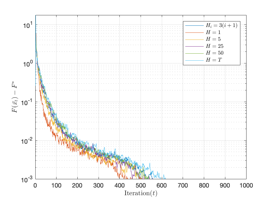
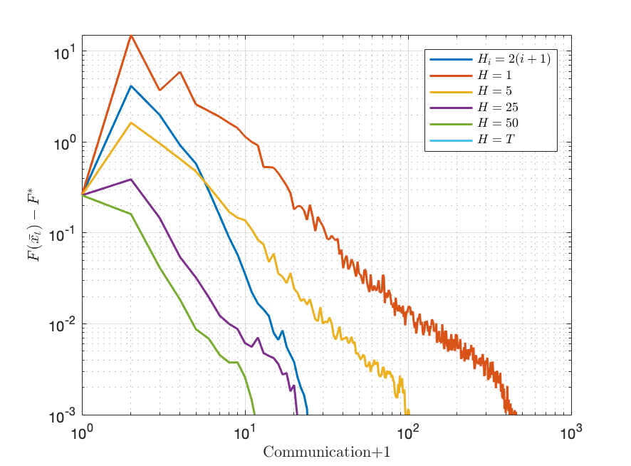
Figure 3(a) shows that all the communication strategies share similar behavior considering error over iterations. This may be due to the fact that for the noise variance the strong-growth condition (Assumption 2) is not satisfied with a significant coefficient . Figure 3(b) shows that when considering error over communications, our proposed strategy remains one of the most competitive.


To evaluate the impact of the number of workers and the communication network structure in Decentralized Local SGD, we generate two sets of communication graphs: various Erds-Rnyi graphs with different number of workers and the probability of connectivity , where is the average degree of nodes and with , indicating a sparse Erds-Rnyi graph, or , indicating a dense Erds-Rnyi graph; various path graphs with different number of workers. We use the local-degree weights to generate the mixing matrix.
We use Decentralized Local SGD (Algorithm 1) to minimize and set the communication strategy to be varying intervals with the number of communication rounds . We select iterations, and the step-size sequence with . We start each simulation from the initial point of and repeat each simulation times. The average of the results are reported in Figures 4(a) and 4(b).
Figures 4(a)(b) show similar patterns as Figures 2(a)(b), and further verify that while graph connectivity may not be the major impact factor of the convergence speed of Decentralized Local SGD, linear-speed up in the number of workers can be expected with only communication rounds.
