跳到论文正文
W Papers独立论文阅读器 arXiv:2011.03074 论文正文 计算阅读时间 · 0%
引用这篇论文根据当前论文元数据生成,正式投稿前建议核对。


Statistical analysis of Wasserstein GANs with applications to time series forecasting

Moritz Haas and Stefan Richter

Abstract

We provide statistical theory for conditional and unconditional Wasserstein generative adversarial networks (WGANs) in the framework of dependent observations. We prove upper bounds for the excess Bayes risk of the WGAN estimators with respect to a modified Wasserstein-type distance. Furthermore, we formalize and derive statements on the weak convergence of the estimators and use them to develop confidence intervals for new observations. The theory is applied to the special case of high-dimensional time series forecasting. We analyze the behavior of the estimators in simulations based on synthetic data and investigate a real data example with temperature data. The dependency of the data is quantified with absolutely regular β\beta-mixing coefficients.

1 Introduction

Generative adversarial networks (GANs) are a class of algorithms in machine learning for learning distributions in high-dimensional feature spaces. After the training process, they are able to generate new random fake observations mimicking the observations already seen. In applications, they have shown to provide surprisingly good results in image and speech generation as well as in inpainting tasks.

The training process is designed as follows: Iteratively, two neural networks compete against each other. While the first network (the generator) produces new random observations which imitate the original training samples, the second network (the critic or discriminator) judges their quality and tries to discriminate between true and generated observations. The assessment is performed with a specific distance of probability distributions. The original GAN was defined with a Kullback-Leibler-type divergence (so called Vanilla GANs, cf. [15]). In practical applications, GANs using the Wasserstein distance (so called WGANs, cf. [4], [16]) have become popular due to their training stability and the high quality of the generated observations. In contrast to other divergence measures, such as the Kullback-Leibler divergence or the total variation divergence, the Wasserstein distance metrizes weak convergence, which makes it sensible to differences of distributions on lower-dimensional submanifolds and with disjoint supports (cf. [4]). This property stabilizes the training procedure of WGANs remarkably.

Let d∈ℕd\in\mathbb{N} be the dimension of the feature space. WGANs learn a structured probability distribution ℙX\mathbb{P}^{X} from potentially high-dimensional training samples Xi∈ℝdX_{i}\in\mathbb{R}^{d}, i∈{1,…,n}i\in\{1,...,n\}. To do so, a latent space ℝdZ\mathbb{R}^{d_{Z}} with dimension dZ∈ℕd_{Z}\in\mathbb{N} and latent random variables Z1,…,Zn∈ℝdZZ_{1},...,Z_{n}\in\mathbb{R}^{d_{Z}} with a given “base distribution” ℙZ\mathbb{P}^{Z} are introduced. Then one tries to minimize the Wasserstein distance of the empirical measure of the training samples,

ℙ^nX:=1n​∑i=1nδXi\hat{\mathbb{P}}_{n}^{X}:=\frac{1}{n}\sum_{i=1}^{n}\delta_{X_{i}}

(here, δXi\delta_{X_{i}} denotes the point measure on XiX_{i}) and the empirical measure of modified latent variables,

ℙ^ng⁡(Z):=1n​∑j=1nδg⁡(Zj),\hat{\mathbb{P}}_{n}^{g(Z)}:=\frac{1}{n}\sum_{j=1}^{n}\delta_{g(Z_{j})},

with respect to the generator g:ℝdZ→ℝdXg:\mathbb{R}^{d_{Z}}\to\mathbb{R}^{d_{X}}. After the learning process, an estimator g^\hat{g} of gg can produce new observations g^​(Z)\hat{g}(Z) which approximately follow ℙX\mathbb{P}^{X} by sampling from the latent space Z∼ℙZZ\sim\mathbb{P}^{Z}.

The approach was generalized to conditional distributions ℙX|Y\mathbb{P}^{X|Y} in [21]. Let dY∈ℕd_{Y}\in\mathbb{N} be the dimension of the conditional feature space. If samples (Xi,Yi)∈ℝd+dY(X_{i},Y_{i})\in\mathbb{R}^{d+d_{Y}}, i∈{1,…,n}i\in\{1,...,n\} are observed, then the conditional WGAN approximately minimizes the Wasserstein distance between the empirical measure

ℙ^nX,Y:=1n​∑i=1nδXi,Yi\hat{\mathbb{P}}_{n}^{X,Y}:=\frac{1}{n}\sum_{i=1}^{n}\delta_{X_{i},Y_{i}}

and

ℙ^ng⁡(Z,Y),Y:=1n​∑i=1nδg⁡(Zi,Yi),Yi,\hat{\mathbb{P}}_{n}^{g(Z,Y),Y}:=\frac{1}{n}\sum_{i=1}^{n}\delta_{g(Z_{i},Y_{i}),Y_{i}},

where here the conditional generator is a function g:ℝdZ+dY→ℝdg:\mathbb{R}^{d_{Z}+d_{Y}}\to\mathbb{R}^{d} which also incorporates the values of YY during evaluation. In the same manner as before, approximate observations from ℙX|Y\mathbb{P}^{X|Y} can be obtained after the learning process (i.e. when an estimate g^\hat{g} of gg is available) by g^​(Z,Y)\hat{g}(Z,Y) with samples Z∼ℙZZ\sim\mathbb{P}^{Z} and given observations YY. In practice, conditional GANs (cGANs) introduce the information Y=yY=y to the generator in various stages of the architecture. cGANs are very popular for generating images given certain labels such as age, gender or glasses [2] and in image-to-image translation tasks (cf. [17, 20]), e.g. colorizing images or reconstructing higher resolution.

In both situations (unconditional and conditional), WGANs provide an approximation of the law of ℙX\mathbb{P}^{X} or ℙX|Y\mathbb{P}^{X|Y} via g^​(Z)\hat{g}(Z) or g^​(Y,Z)\hat{g}(Y,Z) and offer a powerful tool to obtain new samples even if the training data is high-dimensional. The reason is that under appropriate restrictions on the structure of gg and the dimension dZd_{Z} of the latent variables, the data g⁡(Z)g(Z) lies in a low-dimensional submanifold of ℝd\mathbb{R}^{d}.

The purpose of this paper is to provide a theoretical framework for conditional and unconditional WGANs and to prove convergence rates of the excess Bayes risk (with respect to a modified Wasserstein distance) in the context of time series XiX_{i}, i=1,…,ni=1,...,n. We formalize in which sense the learned generator function can be used to provide asymptotic confidence sets for XX. As an application, we will investigate conditional WGANs to provide confidence intervals for observations of high-dimensional time series. The use of WGANs and our corresponding theory is not limited to this example: For instance, one could think of new smoothed Bootstrap techniques.

Recent results from [6] and [7] already provided theoretical results for the excess Bayes risk of GANs and WGANs in the case of i.i.d. observations XiX_{i}. They used network classes fixed in nn for both discriminators and generators and therefore could not derive convergence rates for the whole excess Bayes risk. Furthermore, the minimized objective could not be used to derive (asymptotic) distributional properties of their corresponding estimators g^\hat{g}. With our results, we extend the theory of these publications in several ways:

  1. 1.

    We derive explicit statistical properties like characterization of weak convergence for the modified Wasserstein distance used in WGANs

  2. 2.

    We investigate the conditional WGAN, which is an important generalization for standard statistical applications as forecasting.

  3. 3.

    We allow the generator to be in a Hölder class and explicitly discuss upper bounds for the approximation error of g^\hat{g}. This yields explicit upper bounds on the whole excess Bayes risk and allows a discussion of the impact of structural assumptions on gg and how the curse of dimension can be avoided in practice.

  4. 4.

    We allow the observations XiX_{i}, i=1,…,ni=1,...,n and Yi,i=1,…,nY_{i},i=1,...,n to be dependent.

From a technical point of view, we measure dependence with absolutely regular β\beta-mixing coefficients. We use empirical process theory from [12] and [10] as well as refined Talagrand’s inequalities from [8] to provide large deviation inequalities of the excess Bayes risk.

The paper is organized as follows. In Section 2, we introduce the Wasserstein metric as well as the conditional and unconditional WGAN estimator based on neural networks. Section 3 covers the unconditional case. We firstly relate the introduced modified Wasserstein distance (a network based integral probability metric, cf. [22]) to the 1-Wasserstein distance. Then we provide convergence rates for the excess Bayes risk with respect to this distance under structural assumptions on the underlying data generating process and the neural networks used for estimation. In Section 4 we establish equivalent results for the conditional case. In Section 5, we transfer our results from Section 4 to high-dimensional time series forecasting. In Section 6, we provide simulation results of the conditional WGAN algorithm both for simulated data and real-world temperature data. A short conclusion is drawn in Section 7. All proofs are deferred without further reference to the Appendix.

We now summarize some notation used in this paper. (Ω,𝒜,ℙ)(\Omega,\mathcal{A},\mathds{P}) will denote a Borel probability space. For some vector x∈ℝdx\in\mathbb{R}^{d}, let |x|=(∑j=1d|xj|2)1/2|x|=(\sum_{j=1}^{d}|x_{j}|^{2})^{1/2} denote its Euclidean norm, |x|∞=maxi⁡|xi||x|_{\infty}=\max_{i}|x_{i}| and |x|0=∑i𝟏​(xi≠0)|x|_{0}=\sum_{i}\mathbf{1}(x_{i}\neq 0). For measurable functions f:T→ℝf:T\to\mathbb{R}, we write ‖f‖∞:=supx∈T|f⁡(x)|\|f\|_{\infty}:=\sup_{x\in T}|f(x)| whenever there is no ambiguity on the domain T⊂ℝrT\subset\mathbb{R}^{r}. For f:T→ℝd~f:T\to\mathbb{R}^{\tilde{d}}, we further denote ‖f‖∞:=maxj=1,…,d~⁡‖fj‖∞\|f\|_{\infty}:=\max_{j=1,...,\tilde{d}}\|f_{j}\|_{\infty} and the Lipschitz norm ‖f‖L:=supx≠y|f⁡(x)−f⁡(y)||x−y|\|f\|_{L}:=\sup_{x\not=y}\frac{|f(x)-f(y)|}{|x-y|} we denote the Lipschitz norm w.r.t. the Euclidean norm |⋅||\cdot|. Finally, we use the following multi-index calculus: For differentiable functions f:T→ℝf:T\to\mathbb{R} and α=(α1,…,αr)∈ℕ0r\alpha=(\alpha_{1},\dots,\alpha_{r})\in\mathds{N}_{0}^{r}, let |α|=∑i=1rαi|\alpha|=\sum_{i=1}^{r}\alpha_{i} and let ∂αf=∂1α1…​∂rαrf\partial^{\alpha}f=\partial^{\alpha_{1}}_{1}\dots\partial^{\alpha_{r}}_{r}f denote the rr-th partial derivative. Finally, for real-valued random variables WW and q>0q>0 we write ‖W‖q:=𝔼​[|W|q]1/q\|W\|_{q}:=\mathbb{E}[|W|^{q}]^{1/q}.

2 The Wasserstein GAN estimator

Throughout the paper, we consider XiX_{i}, i=1,…,ni=1,...,n to be a strictly stationary process taking values in [0,1]d[0,1]^{d}, where d∈ℕd\in\mathbb{N} is an arbitrary dimension. Here, we restrict ourselves to the unit cube [0,1]d[0,1]^{d} for convenience, our theory could easily be generalized to arbitrary compact Euclidean spaces. We start with an introduction of the typical approximations used in the Wasserstein GAN approach as well as the optimization problem we aim to discuss. Based on this notation, we then give a statistical formulation of the conditional Wasserstein GAN. To keep our assumptions concise, we define the set of functions f:T⊂ℝr→ℝf:T\subset\mathbb{R}^{r}\to\mathbb{R} with Hölder coefficient β≥1\beta\geq 1 via

Cβ​(T,K)\displaystyle C^{\beta}(T,K)
:⁣=\displaystyle:= {f:T→ℝ|∑α: 0≤|α|<β∥∂αf∥∞+∑α:|α|=β−1supx≠y|∂αf⁡(x)−∂αf⁡(y)||x−y|∞≤K},\displaystyle\big\{f:T\to\mathbb{R}\big|\,\sum_{\alpha:\,0\leq|\alpha|<\beta}\|\partial^{\alpha}f\|_{\infty}+\sum_{\alpha:\,|\alpha|=\beta-1}\sup_{x\neq y}\frac{|\partial^{\alpha}f(x)-\partial^{\alpha}f(y)|}{|x-y|_{\infty}}\leq K\big\},

where K>0K>0.

2.1 Simplification of the WGAN objective and model assumption

Let dZ∈ℕd_{Z}\in\mathbb{N} and ℙZ\mathbb{P}^{Z} a known distribution on [0,1]dZ[0,1]^{d_{Z}}. Let 𝒢⊂{g:ℝdZ→ℝd​ measurable}\mathcal{G}\subset\{g:\mathbb{R}^{d_{Z}}\to\mathbb{R}^{d}\text{ measurable}\} be a space of generators. In this paper, we will assume that 𝒢\mathcal{G} consists of smooth functions with a special structure (this is made precise in Definition 2.1). The objective of a WGAN is to approximate the underlying probability distribution ℙX\mathbb{P}^{X} by minimizing the 1-Wasserstein distance to ℙg⁡(Z)\mathbb{P}^{g(Z)} with respect to g∈𝒢g\in\mathcal{G}. By the Kantorovich-Rubinstein duality (cf. [30]), the 1-Wasserstein distance of two probability distributions ℙ1,ℙ2\mathbb{P}_{1},\mathbb{P}_{2} on ℝd\mathbb{R}^{d} can be written as

W1(ℙ1,ℙ2)=supf:ℝd→ℝ,‖f‖L≤1{∫fdℙ1−∫fdℙ2}.W_{1}(\mathbb{P}_{1},\mathbb{P}_{2})=\sup_{f:\mathbb{R}^{d}\to\mathbb{R},\|f\|_{L}\leq 1}\big\{\int f\,\text{d}\mathbb{P}_{1}-\int f\,\text{d}\mathbb{P}_{2}\big\}.

The original objective of the WGAN is to find a suitable g∈𝒢g\in\mathcal{G} which minimizes

W1(ℙX,ℙg⁡(Z))=supf:ℝd→ℝ,‖f‖L≤1{𝔼f(X)−𝔼f(g(Z))}.W_{1}(\mathds{P}^{X},\mathds{P}^{g(Z)})=\sup_{f:\mathbb{R}^{d}\to\mathbb{R},\|f\|_{L}\leq 1}\big\{\mathbb{E}f(X)-\mathbb{E}f(g(Z))\big\}. (2.1)

In practical applications, the set of critics f:ℝd→ℝf:\mathbb{R}^{d}\to\mathbb{R} is replaced by a certain set of neural networks ℛD⊂{f:ℝd→ℝ}\mathcal{R}_{D}\subset\{f:\mathbb{R}^{d}\to\mathbb{R}\}. This replacement makes the objective more tractable and also allows the graphical interpretation of competing networks. Similarly, for estimation, the set of possible generators 𝒢\mathcal{G} is replaced by a set of neural networks ℛG⊂{f:ℝdZ→ℝd}\mathcal{R}_{G}\subset\{f:\mathbb{R}^{d_{Z}}\to\mathbb{R}^{d}\}.

In the following, we therefore replace the theoretical objective (2.1) by

W1,n​(g):=supf∈ℛD,‖f‖L≤1{𝔼​f​(X)−𝔼​f​(g⁡(Z))}.W_{1,n}(g):=\sup_{f\in\mathcal{R}_{D},\|f\|_{L}\leq 1}\big\{\mathbb{E}f(X)-\mathbb{E}f(g(Z))\big\}. (2.2)

Note that W1,nW_{1,n} may depend on nn through the class ℛD\mathcal{R}_{D}. Due to the restriction on f∈ℛDf\in\mathcal{R}_{D}, one can not expect that W1,n​(g)=W1​(ℙX,ℙg⁡(Z))W_{1,n}(g)=W_{1}(\mathbb{P}^{X},\mathbb{P}^{g(Z)}). This raises the question which properties W1,n​(g)W_{1,n}(g) should preserve (and thus, how large and of which form ℛD\mathcal{R}_{D} should be) to make it a meaningful distance of the measures ℙX\mathbb{P}^{X} and ℙg⁡(Z)\mathbb{P}^{g(Z)}. Our basic aim is to preserve the property that W1,nW_{1,n} characterizes weak convergence in the sense that for any sequence gn∈ℛGg_{n}\in\mathcal{R}_{G},

W1,n​(gn)→0 implies gn​(Z)​→𝑑​X.W_{1,n}(g_{n})\to 0\quad\text{ implies }\quad g_{n}(Z)\overset{d}{\to}X.

The precise conditions on ℛD\mathcal{R}_{D} and its connections to the space ℛG\mathcal{R}_{G} of generators are given in Lemma 3.2 in Section 3.

In [24, Theorem 3] it was shown that the 1-Wasserstein distance between two measures in ℝd\mathbb{R}^{d} can, in general, not be estimated with a better rate than (nlog(n))−1/d(n\log(n))^{-1/d}. Even though W1,n​(g)W_{1,n}(g) is smaller than W1​(ℙX,ℙg⁡(Z))W_{1}(\mathbb{P}^{X},\mathbb{P}^{g(Z)}), one needs specific structural assumptions on the underlying distribution and the class of estimators to overcome the curse of dimension. Since we aim to approximate ℙX\mathbb{P}^{X} by ℙg⁡(Z)\mathbb{P}^{g(Z)}, it is clear that we expect some kind of “sparsity” of XX if dZ<dd_{Z}<d. If we expect ℙX\mathbb{P}^{X} to lie (approximately) in a dgd_{g}-dimensional submanifold (dg∈{1,…,d}d_{g}\in\{1,...,d\}) of ℝd\mathbb{R}^{d}, it seems reasonable to choose dZ=dgd_{Z}=d_{g}. To allow for a more flexible choice of dZd_{Z}, we introduce the following function class.

Definition 2.1 (Generator function class).

Let 𝒢⁡(dZ,dg,β,K)\mathcal{G}(d_{Z},d_{g},\beta,K) be the set of all measurable functions g:ℝdZ→ℝdg:\mathbb{R}^{d_{Z}}\to\mathbb{R}^{d} such that any component only depends on dgd_{g} arguments and lies in Cβ​([0,1]dZ,K)C^{\beta}([0,1]^{d_{Z}},K).

In principle, one can allow for much more complicated structures of the generator functions. Here we reduce ourselves to the above formulation for simplicity. An example of a more general class which has auto-encoder structure is introduced for the conditional case (cf. Definition 2.2) and could also be chosen here.
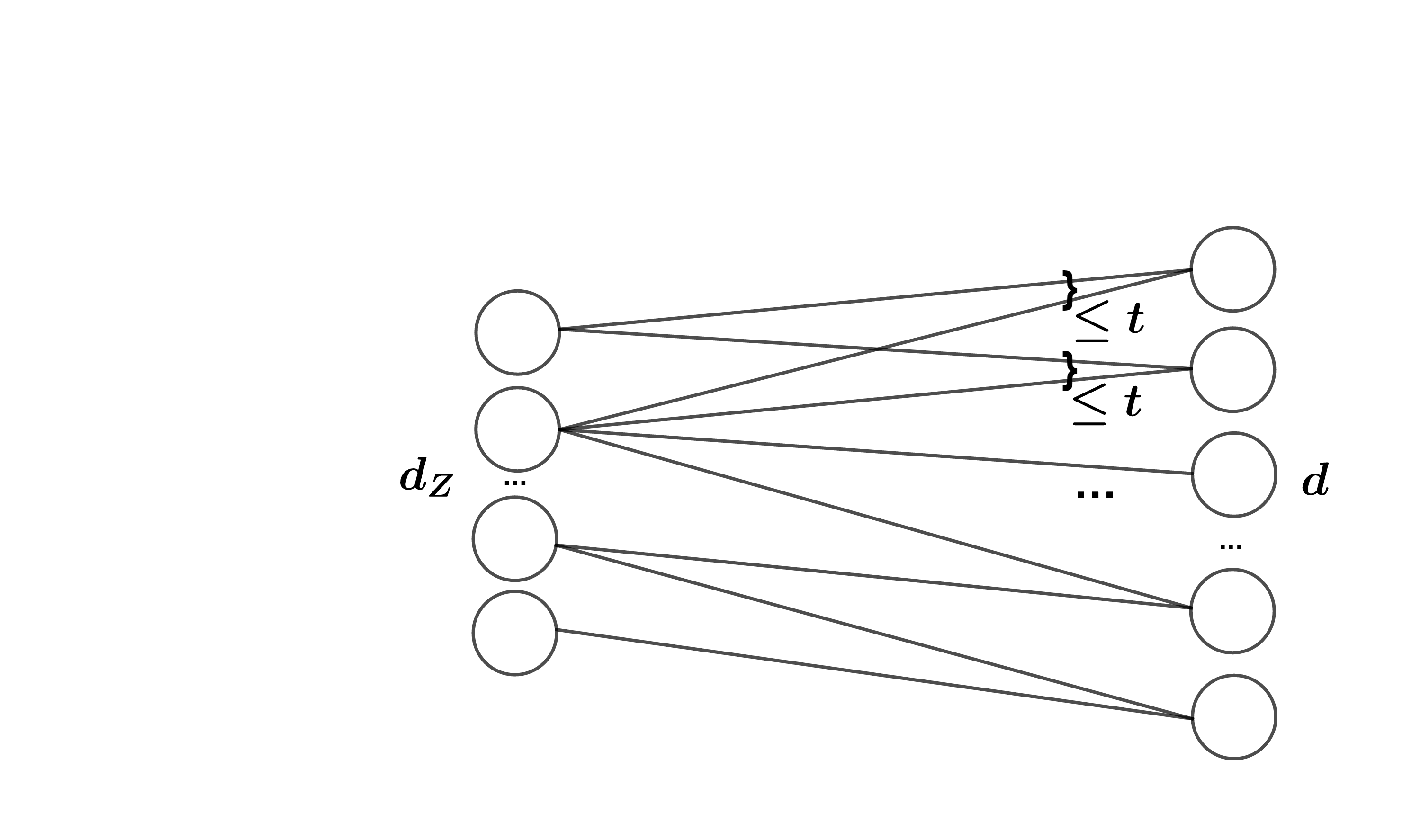
Refer to caption
Figure 1: Structure of the generating functions gg which are used to model the distribution of XX with g⁡(Z)g(Z).

2.2 ReLU neural networks

We now specify the classes ℛD\mathcal{R}_{D} and ℛG\mathcal{R}_{G} of neural networks in more detail. To do so, we use a theoretical formulation from [28]. For x∈ℝx\in\mathbb{R}, let σ⁡(x)=max⁡{x,0}\sigma(x)=\max\{x,0\} denote the rectified linear unit (ReLU) activation function. For v,x∈Rpv,x\in R^{p}, p∈ℕp\in\mathds{N}, define

σv​(x)=σ⁡(x−v),\sigma_{v}(x)=\sigma(x-v),

where σ⁡(⋅)\sigma(\cdot) is applied component-wise to the vector x−vx-v. Let L∈ℕL\in\mathbb{N} and p=(p0,…,pL+1)∈ℕL+2p=(p_{0},...,p_{L+1})\in\mathbb{N}^{L+2}. A neural network with network architecture (L,𝐩)(L,\mathbf{p}) is a function

h:ℝp0→ℝpL+1,h⁡(x)=W(L)​σv(L)​W(L−1)​…​W(1)​σv(1)​W(0)​x,h:\mathbb{R}^{p_{0}}\rightarrow\mathbb{R}^{p_{L+1}},\quad h(x)=W^{(L)}\sigma_{v^{(L)}}W^{(L-1)}\dots W^{(1)}\sigma_{v^{(1)}}W^{(0)}x, (2.3)

where W(l)∈ℝpl×pl+1W^{(l)}\in\mathbb{R}^{p_{l}\times p_{l+1}}, l=0,…,Ll=0,...,L are the weight matrices and v(l)∈ℝplv^{(l)}\in\mathbb{R}^{p_{l}}, l=1,…,Ll=1,...,L are the bias vectors associated to the network. Consequently, let

ℛ(L,𝐩)={h:ℝp0→ℝpL+1|g is of the form (2.3)},\displaystyle\mathcal{R}(L,\mathbf{p})=\Big\{h:\mathbb{R}^{p_{0}}\rightarrow\mathbb{R}^{p_{L+1}}\;|\;\text{$g$ is of the form (\ref{form_network})}\Big\},

be the class of deep ReLU networks with network architecture (L,𝐩)(L,\mathbf{p}). Training of neural networks typically is done with a stochastic gradient descent method and a random initialization of the weight matrices. It is observed in practice that only few parameters of the resulting networks are “active” in the sense that they contribute to the final function value. Accordingly, we introduce the set of sparse networks bounded by F>0F>0 by

ℛ(L,𝐩,s,F):={\displaystyle\mathcal{R}(L,\mathbf{p},s,F):=\Big\{ h∈ℛ⁡(L,𝐩)​|maxj=0,…,L⁡‖Wj‖∞∨|​vj|∞≤1,\displaystyle h\in\mathcal{R}(L,\mathbf{p})\;\Big|\;\max_{j=0,\dots,L}\|W_{j}\|_{\infty}\vee|v_{j}|_{\infty}\leq 1,
∑j=0L∥Wj∥0+|vj|0≤s and ∥|h|∞∥L∞​([0,1]p0)≤F}.\displaystyle\sum_{j=0}^{L}\|W_{j}\|_{0}+|v_{j}|_{0}\leq s\text{ and }\|\;|h|_{\infty}\|_{L^{\infty}([0,1]^{p_{0}})}\leq F\Big\}.

Since FF is fixed, we will abbreviate ℛ⁡(L,𝐩,s)=ℛ⁡(L,𝐩,s,F)\mathcal{R}(L,\mathbf{p},s)=\mathcal{R}(L,\mathbf{p},s,F) in the following.

2.3 The unconditional WGAN estimator

We use the theoretical formulation in (2.2) but replace the expectation 𝔼​f​(X)\mathbb{E}f(X) by its empirical counterpart 1n​∑i=1nf⁡(Xi)\frac{1}{n}\sum_{i=1}^{n}f(X_{i}). Furthermore, 𝔼​f​(g⁡(Z))\mathbb{E}f(g(Z)) is approximated by 1n​ℰ​∑j=1n​ℰf⁡(g⁡(Zi​j))\frac{1}{n\mathcal{E}}\sum_{j=1}^{n\mathcal{E}}f(g(Z_{ij})), where Zi,jZ_{i,j}, j=1,…,ℰj=1,...,\mathcal{E}, i=1,…,ni=1,...,n are i.i.d. realizations of ℙZ\mathbb{P}^{Z} (independent of XiX_{i}, i=1,…,ni=1,...,n) and ℰ∈ℕ\mathcal{E}\in\mathbb{N} is some parameter. We then obtain

g^n:=arg​ming∈ℛ⁡(Lg,𝐩g,sg)⁡W^1,n​(g)\hat{g}_{n}:=\argmin_{g\in\mathcal{R}(L_{g},\mathbf{p}_{g},s_{g})}\hat{W}_{1,n}(g) (2.4)

with

W^1,n​(g)\displaystyle\hat{W}_{1,n}(g) :⁣=\displaystyle:= supf∈ℛ⁡(Lf,𝐩f,sf),‖f‖L≤1{ℙ^nX​f−ℙ^n​ℰZ​(f∘g)}\displaystyle\sup_{f\in\mathcal{R}(L_{f},\mathbf{p}_{f},s_{f}),\|f\|_{L}\leq 1}\big\{\hat{\mathbb{P}}_{n}^{X}f-\hat{\mathbb{P}}_{n\mathcal{E}}^{Z}(f\circ g)\big\}
=\displaystyle= supf∈ℛ⁡(Lf,𝐩f,sf),‖f‖L≤11n​∑i=1n{f⁡(Xi)−1ℰ​∑j=1ℰf⁡(g⁡(Zi,j))}\displaystyle\sup_{f\in\mathcal{R}(L_{f},\mathbf{p}_{f},s_{f}),\|f\|_{L}\leq 1}\frac{1}{n}\sum_{i=1}^{n}\big\{f(X_{i})-\frac{1}{\mathcal{E}}\sum_{j=1}^{\mathcal{E}}f(g(Z_{i,j}))\big\}

where Lg,Lf∈ℕL_{g},L_{f}\in\mathbb{N} are the layer sizes, 𝐩g,𝐩f\mathbf{p}_{g},\mathbf{p}_{f} the corresponding width vectors and sg,sfs_{g},s_{f} the sparsity parameters.

Note that an optimizer g^n\hat{g}_{n} exists (cf. [7]), since W^1,n\hat{W}_{1,n} is Lipschitz continuous with respect to g∈ℛ⁡(Lg,𝐩g,sg)g\in\mathcal{R}(L_{g},\mathbf{p}_{g},s_{g}) and g∈ℛ⁡(Lg,𝐩g,sg)g\in\mathcal{R}(L_{g},\mathbf{p}_{g},s_{g}) is Lipschitz continuous with respect to its parameters W(l)W^{(l)}, v(l)v^{(l)}, which in turn are defined on a compact set. Similarly there exists an optimal critic network in ℛ⁡(Lf,𝐩f,sf)\mathcal{R}(L_{f},\mathbf{p}_{f},s_{f}) for any function g:[0,1]dZ→[0,1]dg:[0,1]^{d_{Z}}\to[0,1]^{d}.

The parameter ℰ\mathcal{E} is motivated by algorithms which are used in practice to find approximations of (2.4), cf. Section 6. These algorithms work iteratively. Each iteration which uses all training data is called epoch. The random variables ZiZ_{i}, i=1,…,ni=1,...,n are not sampled one time at the beginning but new samples are generated in each training epoch. Although in practice the generator only has access to a part of the data XiX_{i}, i=1,…,ni=1,...,n in each epoch, ℰ\mathcal{E} roughly grows proportional to the number of epochs. Thus one can imitate the knowledge coming from the additional realizations of ℙZ\mathbb{P}^{Z} and study its implications.

Appropriate choices for these parameters to guarantee upper bounds for the excess Bayes risk are formulated in Section 3.

2.4 The conditional WGAN estimator

Conditional GANs (cGANs), firstly introduced in [21], extend the task of learning to sample from a given distribution ℙX\mathbb{P}^{X} to learning to sample from conditional distributions PX|Y=yP^{X|Y=y}, y∈[0,1]dYy\in[0,1]^{d_{Y}}, where YY is another random variable in a space [0,1]dY[0,1]^{d_{Y}} encoding some information about XX. The idea is simply to learn the joint distribution ℙX,Y\mathbb{P}^{X,Y} with the same Wasserstein objective (2.1) with a generator that has access to YY. The formal legitimation is that if we find a function gc∗:[0,1]dZ+dY→ℝdg_{c}^{*}:[0,1]^{d_{Z}+d_{Y}}\to\mathbb{R}^{d} with ℙX,Y=ℙgc∗​(Z,Y),Y\mathbb{P}^{X,Y}=\mathbb{P}^{g_{c}^{*}(Z,Y),Y}, then the independency of Y,ZY,Z implies ℙX|Y=y=ℙgc∗​(Z,y)\mathbb{P}^{X|Y=y}=\mathbb{P}^{g_{c}^{*}(Z,y)}.

We introduce a more complex class 𝒢c​(dZ,dY,D,dg,β,K)\mathcal{G}^{c}(d_{Z},d_{Y},D,d_{g},\beta,K) of generators with encoder-decoder structure, cf. Figure 2, so that generators can depend on all components of the conditional information given by YY, even for large dimensions dYd_{Y}.

Definition 2.2 (Encoder-decoder structure).

Let 𝒢c​(dZ,dY,D,dg,β,K)\mathcal{G}^{c}(d_{Z},d_{Y},D,d_{g},\beta,K) be the set of all measurable functions g:ℝdZ+dY→ℝdg:\mathbb{R}^{d_{Z}+d_{Y}}\to\mathbb{R}^{d} which have the form

g=gd​e​c∘ge​n​c,1∘ge​n​c,0,g=g_{dec}\circ g_{enc,1}\circ g_{enc,0},

where

  • •

    ge​n​c,0:ℝdZ+dY→ℝDg_{enc,0}:\mathbb{R}^{d_{Z}+d_{Y}}\to\mathbb{R}^{D} such that any component only depends on dgd_{g} arguments and lies in Cβ​([0,1]dg,K)C^{\beta}([0,1]^{d_{g}},K),

  • •

    ge​n​c,1:ℝD→ℝdgg_{enc,1}:\mathbb{R}^{D}\to\mathbb{R}^{d_{g}} such that any component lies in Cβ~​([0,1]D,K)C^{\tilde{\beta}}([0,1]^{D},K), with some β~≥Ddg​β\tilde{\beta}\geq\frac{D}{d_{g}}\beta.

  • •

    gd​e​c:ℝdg→ℝdg_{dec}:\mathbb{R}^{d_{g}}\to\mathbb{R}^{d} such that any component lies in Cβ​([0,1]dg,K)C^{\beta}([0,1]^{d_{g}},K).

Refer to caption
Figure 2: Structure of the generating functions gg which are used to model the distribution of (X,Y)(X,Y) with (g⁡(Z,Y),Y)(g(Z,Y),Y).

The original objective now is to find a minimizer of

W1,nc​(g):=supf∈ℛ⁡(Lf,𝐩f,sf),‖f‖L≤1{𝔼​f​(X,Y)−𝔼​f​(g⁡(Z,Y),Y)}.W_{1,n}^{c}(g):=\sup_{f\in\mathcal{R}(L_{f},\mathbf{p}_{f},s_{f}),\|f\|_{L}\leq 1}\left\{\mathbb{E}f(X,Y)-\mathbb{E}f\big(g(Z,Y),\,Y\big)\right\}.

If (Xi,Yi)(X_{i},Y_{i}), i=1,…,ni=1,\dots,n are strictly stationary realizations of ℙ(X,Y)\mathbb{P}^{(X,Y)} and ZiZ_{i}, i=1,…,ni=1,...,n are i.i.d. realizations of ℙZ\mathbb{P}^{Z} independent of (Xi,Yi)(X_{i},Y_{i}), i=1,…,ni=1,...,n, we define

g^nc:=arg​ming∈ℛ⁡(Lg,𝐩g,sg)⁡W^1,nc​(g)\hat{g}_{n}^{c}:=\argmin_{g\in\mathcal{R}(L_{g},\mathbf{p}_{g},s_{g})}\hat{W}_{1,n}^{c}(g) (2.5)

with

W^1,nc​(g)\displaystyle\hat{W}_{1,n}^{c}(g) :⁣=\displaystyle:= supf∈ℛ⁡(Lf,𝐩f,sf),‖f‖L≤11n​∑i=1n{f⁡(Xi,Yi)−f⁡(g⁡(Zi,Yi),Yi)}\displaystyle\sup_{f\in\mathcal{R}(L_{f},\mathbf{p}_{f},s_{f}),\|f\|_{L}\leq 1}\frac{1}{n}\sum_{i=1}^{n}\big\{f(X_{i},Y_{i})-f(g(Z_{i},Y_{i}),Y_{i})\big\}

where Lg,Lf∈ℕL_{g},L_{f}\in\mathbb{N} are the layer sizes, 𝐩g,𝐩f\mathbf{p}_{g},\mathbf{p}_{f} the corresponding width vectors and sg,sfs_{g},s_{f} the sparsity parameters. Appropriate choices for these parameters to guarantee upper bounds for the excess Bayes risk are formulated in Section 4. Note that in contrast to the unconditional WGAN, we do not implement the additional realizations of ℙZ\mathbb{P}^{Z} which may occur in practical algorithms. The reason is that for the conditional WGAN, the observations YiY_{i} in the second summand in W^1,nc​(g)\hat{W}_{1,n}^{c}(g) restrict the use of additional knowledge from ZZ without rather technical assumptions on the structure of gg.

3 Theoretical results for the unconditional WGAN

The first part of this section is devoted to the properties of the modified distances W1,n​(g)W_{1,n}(g). We show connections between W1,n​(g)W_{1,n}(g) and distances which do not depend on nn and prove that under certain assumptions on the set of networks ℛD​(Lf,𝐩f,sf)\mathcal{R}_{D}(L_{f},\mathbf{p}_{f},s_{f}), W1,n​(g)W_{1,n}(g) characterizes weak convergence.

In the second part, we provide upper bounds and convergence rates for the excess Bayes risk

Rn​(g):=W1,n​(g)−infg∈𝒢⁡(dZ,dg,β,K)W1,n​(g)R_{n}(g):=W_{1,n}(g)-\inf_{g\in\mathcal{G}(d_{Z},d_{g},\beta,K)}W_{1,n}(g) (3.1)

for the unconditional WGAN estimator g^n\hat{g}_{n} under assumptions on the network structure. In the third part, we summarize the results to provide asymptotic confidence intervals.

3.1 Properties of the modified Wasserstein distance

We first investigate the connection of W1,n​(g)W_{1,n}(g) to

W1γ​(g):=supf∈Cγ​([0,1]d,K),‖f‖L≤1{𝔼​f​(X)−𝔼​f​(g⁡(Z))}.W_{1}^{\gamma}(g):=\sup_{f\in C^{\gamma}([0,1]^{d},K),\|f\|_{L}\leq 1}\big\{\mathbb{E}f(X)-\mathbb{E}f(g(Z))\big\}.

In opposite to W1,nW_{1,n}, the quantity W1γW_{1}^{\gamma} does not depend on nn and therefore can be seen as a more “stable” distance measure for ℙX\mathbb{P}^{X} towards ℙg⁡(Z)\mathbb{P}^{g(Z)}. Note that

W1γ​(g)\displaystyle W_{1}^{\gamma}(g) ≤\displaystyle\leq W1,n​(g)+2​supf∈Cγ​([0,1]d,K)inff~∈ℛ⁡(Lf,𝐩f,sf)‖f−f~‖∞.\displaystyle W_{1,n}(g)+2\sup_{f\in C^{\gamma}([0,1]^{d},K)}\inf_{\tilde{f}\in\mathcal{R}(L_{f},\mathbf{p}_{f},s_{f})}\|f-\tilde{f}\|_{\infty}.

Using approximation results for neural networks from [28] (cf. Theorem B.2 in the Appendix), one obtains the following result.

Lemma 3.1 (Lower bound on W1,nW_{1,n}).

Let an=n−2​γ2​γ+da_{n}=n^{-\frac{2\gamma}{2\gamma+d}}, and suppose that

  • •

    F≥1F\geq 1,

  • •

    Lf≥log2⁡(n)​log2⁡(4​d∨4​γ)L_{f}\geq\log_{2}(n)\log_{2}(4d\vee 4\gamma),

  • •

    mini=1,…,L⁡pf,i≳n​an\min_{i=1,...,L}p_{f,i}\gtrsim na_{n}

  • •

    sf≳log⁡(n)​n​ans_{f}\gtrsim\log(n)na_{n},

where the constants in the asymptotic expression above depend on γ,d\gamma,d. Then there exists some constants C>0,K∈(0,1)C>0,K\in(0,1) only depending on γ,d,F\gamma,d,F such that

supf∈Cγ​([0,1]d,K),‖f‖L≤1inff~∈ℛD​(Lf,𝐩f,sf)‖f−f~‖∞≤C​an1/2.\sup_{f\in C^{\gamma}([0,1]^{d},K),\|f\|_{L}\leq 1}\inf_{\tilde{f}\in\mathcal{R}_{D}(L_{f},\mathbf{p}_{f},s_{f})}\|f-\tilde{f}\|_{\infty}\leq Ca_{n}^{1/2}.

Especially, for any measurable g:ℝdZ→ℝdg:\mathbb{R}^{d_{Z}}\to\mathbb{R}^{d},

W1γ​(g)≤W1,n​(g)+C​an1/2.W_{1}^{\gamma}(g)\leq W_{1,n}(g)+Ca_{n}^{1/2}. (3.2)

The lemma shows that the convergence rate of W1,n​(g^n)W_{1,n}(\hat{g}_{n}) transfers to W1γ​(g^n)W^{\gamma}_{1}(\hat{g}_{n}) as long as an1/2≤W1,n​(g^n)a_{n}^{1/2}\leq W_{1,n}(\hat{g}_{n}). In fact, this imposes a lower bound on the Hölder exponent γ\gamma of functions considered with W1γW^{\gamma}_{1}.

In the case that ℙX=ℙg∗​(Z)\mathbb{P}^{X}=\mathbb{P}^{g^{*}(Z)} with some g∗∈𝒢⁡(dZ,dg,β,K)g^{*}\in\mathcal{G}(d_{Z},d_{g},\beta,K), the results for the excess Bayes risk (3.1) presented in the following Section 3.2 can be used to derive weak convergence. The reasoning is as follows: If Rn​(g^n)→0R_{n}(\hat{g}_{n})\to 0, then 𝔼​W1,n​(g^n)→0\mathbb{E}W_{1,n}(\hat{g}_{n})\to 0. Then the following lemma can be used.

Lemma 3.2 (Characterization of weak convergence).

Suppose that ℙX=ℙg∗​(Z)\mathbb{P}^{X}=\mathbb{P}^{g^{*}(Z)} for some g∗∈𝒢⁡(dZ,dg,β,K)g^{*}\in\mathcal{G}(d_{Z},d_{g},\beta,K) and let the assumptions of Lemma 3.1 hold with some γ≥1\gamma\geq 1. Let (g^n)n∈ℕ(\hat{g}_{n})_{n\in\mathbb{N}} be a sequence of random variables with 𝔼​W1,n​(g^n)→0\mathbb{E}W_{1,n}(\hat{g}_{n})\to 0. Then

g^n​(Z)​→𝑑​g∗​(Z)=X.\hat{g}_{n}(Z)\overset{d}{\to}g^{*}(Z)=X.

The lemma basically follows from Lemma 3.1 and the fact that Cγ​([0,1]d)C^{\gamma}([0,1]^{d}) forms a convergence-determining class.

Remark 3.3.

Lemma 3.2 implies weak convergence of ℙg^n​(Z)\mathbb{P}^{\hat{g}_{n}(Z)} towards ℙX\mathbb{P}^{X}, but it does not give any information about the speed of convergence. Nevertheless it seems reasonable that the speed depends on the upper bound in (3.2) which is given by the two summands W1,n​(g)W_{1,n}(g) and an1/2a_{n}^{1/2}. Therefore, one should choose γ≥1\gamma\geq 1 large enough such that an1/2≲W1,n​(g)a_{n}^{1/2}\lesssim W_{1,n}(g). This is done in Remark 3.5 below. On the other hand, for larger γ\gamma, W1γ​(g)W_{1}^{\gamma}(g) gives less information about the distance between ℙg⁡(Z)\mathbb{P}^{g(Z)} and ℙX\mathbb{P}^{X}. It is an open question how an optimal balance of γ\gamma should be chosen. A more detailed analysis of the approximation quality of the set of critic networks ℛD​(Lf,𝐩f,sf)\mathcal{R}_{D}(L_{f},\mathbf{p}_{f},s_{f}) could yield more insight. However, this would need sharp upper bounds on the Lipschitz constants of ℛ⁡(Lf,𝐩f,sf)\mathcal{R}(L_{f},\mathbf{p}_{f},s_{f}) and is a pure approximation problem, which is out of the scope of this paper.

3.2 Excess Bayes risk

To state the theoretical results on the excess Bayes risk Rn​(g^n)R_{n}(\hat{g}_{n}) in (3.1), we have to quantify the dependence structure of XiX_{i}, i=1,…,ni=1,\dots,n and YiY_{i}, i=1,…,ni=1,...,n. Basically, observations obtained at time steps which are far away from each other have to be “asymptotically independent”. There exists a large variety of weak and strong mixing conditions. We refer to [9] for a detailed summary of conditions and basic properties. Here, we use absolutely regular β\beta-mixing due to the well-established empirical process theory (cf. [12] and [10]).

The β\beta-mixing coefficient between two σ\sigma-algebras 𝒰,𝒱⊆𝒜\mathcal{U},\mathcal{V}\subseteq\mathcal{A} is defined by

β⁡(𝒰,𝒱):=12​sup∑(i,j)∈I×J|ℙ⁡(Ui∩Vj)−ℙ⁡(Ui)​ℙ​(Vj)|,\beta(\mathcal{U},\mathcal{V}):=\frac{1}{2}\sup\sum_{(i,j)\in I\times J}\big|\mathds{P}(U_{i}\cap V_{j})-\mathds{P}(U_{i})\mathds{P}(V_{j})\big|,

where the supremum is taken over all finite partitions (Ai)(A_{i}) and (Bj)(B_{j}) 𝒰\mathcal{U}- and 𝒱\mathcal{V}-measurable respectively. For a time series XiX_{i}, i=1,…,ni=1,...,n, one defines

βX​(0)=1,βX​(n):=β⁡(σ⁡(Xi,i≤0),σ⁡(Xi,i≥n)),n∈ℕ.\beta_{X}(0)=1,\quad\beta_{X}(n):=\beta\big(\sigma({X}_{i};\,i\leq 0),\sigma({X}_{i};\,i\geq n)\big),\quad n\in\mathds{N}.

Prominent examples of absolutely regular sequences are GARCH and ARMA as well as linear processes (cf. [14, 9, 11]).

We now present the theoretical result for the excess Bayes risk for the unconditional WGAN estimator g^n\hat{g}_{n}.

Theorem 3.4.

Let ϕn=(n​ℰ)−2​β2​β+dg\phi_{n}=(n\mathcal{E})^{-\frac{2\beta}{2\beta+d_{g}}}. Suppose that F≥K∨1F\geq K\vee 1, and

  • (i)

    log2⁡(n​ℰ)​log2⁡(4​dg∨4​β)≤Lg≲log⁡(n​ℰ)\log_{2}(n\mathcal{E})\log_{2}(4d_{g}\vee 4\beta)\leq L_{g}\lesssim\log(n\mathcal{E}),

  • (ii)

    m​i​ni=1,…,Lg​pg,i≳n​ℰ​ϕnmin_{i=1,...,L_{g}}p_{g,i}\gtrsim n\mathcal{E}\phi_{n},

  • (iii)

    sg≍n​ℰ​ϕn​log⁡(n​ℰ)s_{g}\asymp n\mathcal{E}\phi_{n}\log(n\mathcal{E})

  • (iv)

    Lf≤LgL_{f}\leq L_{g}, sf≤sgs_{f}\leq s_{g}.

Suppose that there exist constants κ>1,α>1\kappa>1,\alpha>1 such that for all k∈ℕk\in\mathbb{N}, βX​(k)≤κ⋅k−α\beta_{X}(k)\leq\kappa\cdot k^{-\alpha}. Then

𝔼​Rn​(g^n)≲(sf​Lf​log⁡(sf​Lf)n)1/2+ϕn1/2​log⁡(n​ℰ)3/2,\mathbb{E}R_{n}(\hat{g}_{n})\lesssim\Big(\frac{s_{f}L_{f}\log(s_{f}L_{f})}{n}\Big)^{1/2}+\phi_{n}^{1/2}\log(n\mathcal{E})^{3/2}, (3.3)

and with probability at least 1−4​n−1−2​(log⁡(n)n)α−121-4n^{-1}-2(\frac{\log(n)}{n})^{\frac{\alpha-1}{2}},

Rn​(g^n)≲(sf​Lf​log⁡(sf​Lf)n)1/2+ϕn1/2​log⁡(n​ℰ)3/2+(log⁡(n)n)1/2,R_{n}(\hat{g}_{n})\lesssim\Big(\frac{s_{f}L_{f}\log(s_{f}L_{f})}{n}\Big)^{1/2}+\phi_{n}^{1/2}\log(n\mathcal{E})^{3/2}+\Big(\frac{\log(n)}{n}\Big)^{1/2},

where the bounding constants may depend on characteristics of X1X_{1}, κ,α\kappa,\alpha and d,dZ,dg,β,K,Fd,d_{Z},d_{g},\beta,K,F.

Remark on dependency. Let us discuss this result in more detail. First note that we basically only need that βX​(k)\beta_{X}(k) is summable. The specific polynomial rate of the decay only enters the large deviation result, and is negligible if α≥3\alpha\geq 3. The statistical bounds are obtained by using empirical process theory for absolutely regular β\beta-mixing sequences and refined versions of Talagrand’s inequality for independent variables from [18].

Remark on critic networks. The rate in (3.3) decomposes into two terms, where the first term is determined by properties of the critic networks and the second term stems from generator networks. Regarding the first term, the only condition on the critic functions is given in (iv) which asks that the critic networks allow for less non-zero parameters and have less layers than the generator networks. The lack of conditions is clear since there is no a priori approximation task the critic networks have to fulfill in W1,nW_{1,n}. However, there is some interest in allowing for a large critic function class ℛ⁡(Lf,𝐩f,sf)\mathcal{R}(L_{f},\mathbf{p}_{f},s_{f}) due to the results from Lemma 3.1. This is discussed in more detail in Remark 3.5.

Remark on conditions. Assumptions (i)-(iii) stated in Theorem 3.4 are conditions on the network structure of the generator networks which are allowed (and needed) to grow with nn. Basically, the lower bounds on Lg,𝐩g,sgL_{g},\mathbf{p}_{g},s_{g} are used to bound the approximation error of finding an element g~∈ℛG​(Lg,𝐩g,sg)\tilde{g}\in\mathcal{R}_{G}(L_{g},\mathbf{p}_{g},s_{g}) which approximates g∈𝒢⁡(dZ,dg,β,K)g\in\mathcal{G}(d_{Z},d_{g},\beta,K) well, while the upper bounds control the estimation error.

(i),(iii) ask the generator networks to have approximately log2⁡(n​ℰ)\log_{2}(n\mathcal{E}) layers and allow for approximately

n​ℰ​ϕn​log⁡(n​ℰ)=(n​ℰ)dg2​β+dg​log⁡(n​ℰ)n\mathcal{E}\phi_{n}\log(n\mathcal{E})=(n\mathcal{E})^{\frac{d_{g}}{2\beta+d_{g}}}\log(n\mathcal{E})

non-zero parameters (that is, entries in weight matrices and bias vectors). (ii) asks the layers to have a certain minimal width. Letting the minimal width of all layers grow polynomially in nn seems rather unusual from a practical point of view. This is only due to the approximation technique adopted from [28] and can be improved.

Remark on convergence rate - dimensionality. In [19, Theorem 1] (cf. also [23]) it was shown that β\beta-Hölder smooth densities in the space ℝd\mathbb{R}^{d} can be estimated with a rate not faster than n−β+12​β+dn^{-\frac{\beta+1}{2\beta+d}} with respect to the Wasserstein distance. Note the additional β+1\beta+1 in the nominator instead of β\beta as it is the case, for instance, in standard nonparametric density estimation. Due to the additional structural assumptions, out method yields (up to a log factor) a convergence rate ϕn=n−β2​β+dg\phi_{n}=n^{-\frac{\beta}{2\beta+d_{g}}} with respect to the modified Wasserstein-distance W1,n​(g^n)W_{1,n}(\hat{g}_{n}). It does not depend on the underlying dimensionality dZd_{Z} of the generation space nor the dimension dd of the observation space but only on the reduced dimension dg≤dZd_{g}\leq d_{Z}. Even if dZd_{Z} is chosen large (as it may occur in practice), the generator network estimator g^n\hat{g}_{n} can adapt to the unknown number dgd_{g} of relevant arguments without suffering from a curse of dimension.

Remark on convergence rate - generator size. In practice, along with each sampled batch of data one batch of generated data Zi​1Z_{i1}, i=1,…,ni=1,...,n is produced, so that during the first epoch of training it holds that ℰ=1\mathcal{E}=1. In subsequent epochs, the data set of fixed size nn is reused, while the number of generated samples keeps growing. If we assume that the generator networks approximate the empirical optimizers at each step, the variable ℰ\mathcal{E} introduced in the estimator g^n\hat{g}_{n} can be roughly seen as the number of training epochs and indicates that more and more realizations of ℙZ\mathbb{P}^{Z} are available to train g^n\hat{g}_{n}. In principle, ℰ\mathcal{E} can be chosen arbitrarily large, therefore one can use arbitrarily large generator architectures as long as one generates enough samples during training. Then the performance saturates due to the limited data samples nn and the corresponding discriminator architecture (cf. (3.3)), but not due to the generator capacity. However, note that one cannot directly take ℰ\mathcal{E} as the number of epochs. The reason is that in each epoch, the generator only sees a part of the data XiX_{i}, i=1,…,ni=1,\dots,n (see Table 1).

Remark 3.5 (Selection of critic and generator).

If there exists g∗∈𝒢⁡(dZ,dg,β,K)g^{*}\in\mathcal{G}(d_{Z},d_{g},\beta,K) with ℙg∗​(Z)=ℙX\mathbb{P}^{g^{*}(Z)}=\mathbb{P}^{X}, then the results of Theorem 3.4, (3.3) and Lemma 3.1, (3.2) can be combined. In this case, one could ask for a suitable choice of γ≥1\gamma\geq 1 such that the rates coincide, that is, an=ϕna_{n}=\phi_{n}. This then also leads to more precise conditions on the discriminator network through Lemma 3.1. For simplicity, choose ℰ=1\mathcal{E}=1. We see that equality is obtained with

β2​β+dg=γ2​γ+d,\frac{\beta}{2\beta+d_{g}}=\frac{\gamma}{2\gamma+d},

which is fulfilled for γ=β​ddg\gamma=\beta\frac{d}{d_{g}}, and leads to

𝔼​W1γ​(g^n)≲ϕn1/2​log⁡(n)3/2.\mathbb{E}W^{\gamma}_{1}(\hat{g}_{n})\lesssim\phi_{n}^{1/2}\log(n)^{3/2}.

3.3 Asymptotic confidence intervals

Based on the weak convergence, one can provide asymptotic confidence sets for XX to a given level α\alpha. For simplicity, suppose that XX is one-dimensional. For N∈ℕN\in\mathbb{N}, let Zj∗,j=1,…,NZ_{j}^{*},j=1,...,N be i.i.d. samples of ℙZ\mathbb{P}^{Z}, independent of Xi,Zi​jX_{i},Z_{ij} used to calculate the WGAN estimator g^n\hat{g}_{n} from (2.4). Define the empirical distribution function

F^N,n(x):=1N∑j=1N𝟙{g^n(Zj∗)≤x}\hat{F}_{N,n}(x):=\frac{1}{N}\sum_{j=1}^{N}\mathbbm{1}_{\{\hat{g}_{n}(Z_{j}^{*})\leq x\}}

and let FXF_{X} denote the distribution function of XX. Then the following result holds.

Lemma 3.6.

Suppose that ℙX=ℙg∗​(Z)\mathbb{P}^{X}=\mathbb{P}^{g^{*}(Z)} for some g∗∈𝒢⁡(dZ,dg,β,K)g^{*}\in\mathcal{G}(d_{Z},d_{g},\beta,K) and that ℙX\mathbb{P}^{X} is continuous. Let the assumptions of Lemma 3.1 with some γ≥1\gamma\geq 1 and Theorem 3.4 hold. Then for any ρ>0\rho>0,

lim supn→∞lim supN→∞ℙ⁡(|F^N,n​(X)−FX​(X)|≥ρ)=0.\limsup_{n\to\infty}\limsup_{N\to\infty}\mathbb{P}(|\hat{F}_{N,n}(X)-F_{X}(X)|\geq\rho)=0.

By the probability integral transform, this shows that F^N,n​(X)\hat{F}_{N,n}(X) converges in probability to a uniform distribution on [0,1][0,1]. For fixed α∈(0,1)\alpha\in(0,1), this justifies that the interval

In,N:={x∈ℝ:F^N,n(x)∈(α2,1−α2]}I_{n,N}:=\Big\{x\in\mathbb{R}:\hat{F}_{N,n}(x)\in\left(\frac{\alpha}{2},1-\frac{\alpha}{2}\right]\Big\} (3.4)

which is built from the empirical α2\frac{\alpha}{2} and (1−α2)(1-\frac{\alpha}{2}) quantile curves of g^n​(Zj∗)\hat{g}_{n}(Z_{j}^{*}), j=1,…,Nj=1,...,N is an asymptotic (1−α)(1-\alpha)-confidence set for XX since

ℙ(X∈In,N)=ℙ(F^N,n(X)∈(α2,1−α2])≈ℙ(FX(X)∈(α2,1−α2])=1−α.\mathbb{P}(X\in I_{n,N})=\mathbb{P}\left(\hat{F}_{N,n}(X)\in\left(\frac{\alpha}{2},1-\frac{\alpha}{2}\right]\right)\approx\mathbb{P}\left(F_{X}(X)\in\left(\frac{\alpha}{2},1-\frac{\alpha}{2}\right]\right)=1-\alpha.

4 Theoretical results for the conditional WGAN

4.1 Results for the modified conditional Wasserstein distance

We now provide similar results as given in Lemma 3.1 and Lemma 3.2 for the conditional WGAN formulation.

In analogy, firstly define,

W1c,γ​(g):=supf∈Cγ​([0,1]d+dY,K),‖f‖L≤1{𝔼​f​(X,Y)−𝔼​f​(g⁡(Z,Y),Y)}.W_{1}^{c,\gamma}(g):=\sup_{f\in C^{\gamma}([0,1]^{d+d_{Y}},K),\|f\|_{L}\leq 1}\big\{\mathbb{E}f(X,Y)-\mathbb{E}f(g(Z,Y),Y)\big\}.

Since we use the same approximation result [28], the connection of W1,nc​(g)W^{c}_{1,n}(g) to W1c,γ​(g)W_{1}^{c,\gamma}(g) is essentially the same as in the unconditional case and we omit a proof.

Lemma 4.1.

Let an=n−2​γ2​γ+d+dYa_{n}=n^{-\frac{2\gamma}{2\gamma+d+d_{Y}}}, and suppose that

  • •

    F≥1F\geq 1,

  • •

    Lf≥log2⁡(n)​log2⁡(4​(d+dY)∨4​γ)L_{f}\geq\log_{2}(n)\log_{2}(4(d+d_{Y})\vee 4\gamma),

  • •

    mini=1,…,L⁡pf,i≳n​an\min_{i=1,...,L}p_{f,i}\gtrsim na_{n}

  • •

    sf≳log⁡(n)​n​ans_{f}\gtrsim\log(n)na_{n},

where the constants in the asymptotic expression above depend on γ,d,dY\gamma,d,d_{Y}. Then there exists some constants C>0,K∈(0,1)C>0,K\in(0,1) only depending on γ,d,dY,F\gamma,d,d_{Y},F such that

supf∈Cγ​([0,1]d+dY,K),‖f‖L≤1inff~∈ℛD​(Lf,𝐩f,sf)‖f−f~‖∞≤C​an1/2.\sup_{f\in C^{\gamma}([0,1]^{d+d_{Y}},K),\|f\|_{L}\leq 1}\inf_{\tilde{f}\in\mathcal{R}_{D}(L_{f},\mathbf{p}_{f},s_{f})}\|f-\tilde{f}\|_{\infty}\leq Ca_{n}^{1/2}.

Especially, for any measurable g:ℝdZ→ℝdg:\mathbb{R}^{d_{Z}}\to\mathbb{R}^{d},

W1c,γ​(g)≤W1,nc​(g)+C​an1/2.W_{1}^{c,\gamma}(g)\leq W^{c}_{1,n}(g)+Ca_{n}^{1/2}. (4.1)

In the case that ℙX,Y=ℙg∗​(Z,Y),Y\mathbb{P}^{X,Y}=\mathbb{P}^{g^{*}(Z,Y),Y} with some g∗∈𝒢c​(dZ,dY,D,dg,β,K)g^{*}\in\mathcal{G}^{c}(d_{Z},d_{Y},D,d_{g},\beta,K), the results for the excess Bayes risk (4.3) presented in the following Section 4.2 can be used to derive weak convergence with the help of the following lemma.

Lemma 4.2.

Suppose that ℙX,Y=ℙg∗​(Z,Y),Y\mathbb{P}^{X,Y}=\mathbb{P}^{g^{*}(Z,Y),Y} for some g∗∈𝒢c​(dZ,dY,D,dg,β,K)g^{*}\in\mathcal{G}^{c}(d_{Z},d_{Y},D,d_{g},\beta,K) and let the assumptions of Lemma 3.1 hold with some γ≥1\gamma\geq 1. Let (g^nc)n∈ℕ(\hat{g}^{c}_{n})_{n\in\mathbb{N}} be a sequence of random variables with 𝔼​W1,nc​(g^nc)→0\mathbb{E}W^{c}_{1,n}(\hat{g}_{n}^{c})\to 0. Then

g^nc​(Z,Y)​→𝑑​g∗​(Z,Y)=X.\hat{g}^{c}_{n}(Z,Y)\overset{d}{\to}g^{*}(Z,Y)=X. (4.2)

The lemma basically follows from 4.1 and the fact that Cγ​([0,1]d+dY)C^{\gamma}([0,1]^{d+d_{Y}}) forms a convergence-determining class. Remark 3.3 applies here as well. Moreover, from (4.2) one directly obtains the convergence of ℙg^nc​(Z,y)\mathbb{P}^{\hat{g}^{c}_{n}(Z,y)} towards the conditional distribution ℙX|Y=y\mathbb{P}^{X|Y=y}.

4.2 Excess Bayes risk

We now provide a result for the excess Bayes risk of the conditional WGAN,

Rnc​(g):=W1,nc​(g)−infg∈𝒢⁡(dZ,dY,D,dg,β,K)W1,nc​(g).R_{n}^{c}(g):=W_{1,n}^{c}(g)-\inf_{g\in\mathcal{G}(d_{Z},d_{Y},D,d_{g},\beta,K)}W_{1,n}^{c}(g). (4.3)
Theorem 4.3.

Let ϕn=n−2​β2​β+dg\phi_{n}=n^{-\frac{2\beta}{2\beta+d_{g}}} and β~≥Ddg​β\tilde{\beta}\geq\frac{D}{d_{g}}\beta. Suppose that F≥K∨1F\geq K\vee 1, and

  • (i)

    log2⁡(n)​(2​log2⁡(4​dg∨4​β)+log2⁡(4​D∨4​β~))≤Lg≲log⁡(n)\log_{2}(n)\big(2\log_{2}(4d_{g}\vee 4\beta)+\log_{2}(4D\vee 4\tilde{\beta})\big)\leq L_{g}\lesssim\log(n),

  • (ii)

    m​i​ni=1,…,Lg​pg,i≳n​ϕnmin_{i=1,...,L_{g}}p_{g,i}\gtrsim n\phi_{n},

  • (iii)

    sg≍n​ϕn​log⁡(n)s_{g}\asymp n\phi_{n}\log(n)

  • (iv)

    Lf≤LgL_{f}\leq L_{g}, sf≤sgs_{f}\leq s_{g}.

Suppose that there exist constants κ>1,α>1\kappa>1,\alpha>1 such that for all k∈ℕk\in\mathbb{N}, βX,Y​(k)≤κ⋅k−α\beta_{X,Y}(k)\leq\kappa\cdot k^{-\alpha}. Then

𝔼​Rnc​(g^nc)≲(sf​Lf​log⁡(sf​Lf)n)1/2+ϕn1/2​log⁡(n)3/2,\mathbb{E}R^{c}_{n}(\hat{g}^{c}_{n})\lesssim\Big(\frac{s_{f}L_{f}\log(s_{f}L_{f})}{n}\Big)^{1/2}+\phi_{n}^{1/2}\log(n)^{3/2}, (4.4)

and with probability at least 1−4​n−1−2​(log⁡(n)n)α−121-4n^{-1}-2(\frac{\log(n)}{n})^{\frac{\alpha-1}{2}},

Rnc​(g^nc)≲(sf​Lf​log⁡(sf​Lf)n)1/2+ϕn1/2​log⁡(n)3/2+(log⁡(n)n)1/2,R^{c}_{n}(\hat{g}^{c}_{n})\lesssim\Big(\frac{s_{f}L_{f}\log(s_{f}L_{f})}{n}\Big)^{1/2}+\phi_{n}^{1/2}\log(n)^{3/2}+\Big(\frac{\log(n)}{n}\Big)^{1/2},

where the bounding constants may depend on characteristics of (X1,Y1)(X_{1},Y_{1}) and κ,α,d,dZ,dY,D,dg,β,β~,K,F\kappa,\alpha,d,d_{Z},d_{Y},D,d_{g},\beta,\tilde{\beta},K,F.

All remarks for 3.4 apply here as well.

4.3 Asymptotic confidence intervals

For simplicity, suppose that XX is one-dimensional. For N∈ℕN\in\mathbb{N}, let Zj∗,j=1,…,NZ_{j}^{*},j=1,...,N be i.i.d. samples of ℙZ\mathbb{P}^{Z}, independent of Xi,Yi,ZiX_{i},Y_{i},Z_{i} used to calculate the WGAN estimator g^nc\hat{g}_{n}^{c} from (2.5). Define the empirical distribution function

F^N,nc(x|y):=1N∑j=1N𝟙{g^nc(Zj∗,y)≤x}\hat{F}_{N,n}^{c}(x|y):=\frac{1}{N}\sum_{j=1}^{N}\mathbbm{1}_{\{\hat{g}_{n}^{c}(Z_{j}^{*},y)\leq x\}}

and let FX​(x|y)=ℙ⁡(X≤x|Y=y)F_{X}(x|y)=\mathbb{P}(X\leq x|Y=y) denote the distribution function of XX conditional on Y=yY=y. The proof of the following result is similar to Lemma 4.2 and therefore omitted.

Lemma 4.4.

Suppose that ℙ(X,Y)=ℙ(g∗​(Z,Y),Y)\mathbb{P}^{(X,Y)}=\mathbb{P}^{(g^{*}(Z,Y),Y)} for some g∗∈𝒢⁡(dZ,dY,dg,D,β,K)g^{*}\in\mathcal{G}(d_{Z},d_{Y},d_{g},D,\beta,K) and that FX​(x|y)F_{X}(x|y) is continuous for ℙY\mathbb{P}^{Y}-a.e. yy. Let the assumptions of Lemma 4.1 with some γ≥1\gamma\geq 1 and Theorem 4.3 hold. Then for any ρ>0\rho>0 and for ℙY\mathbb{P}^{Y}-a.e. yy,

lim supn→∞lim supN→∞ℙ⁡(|F^N,n​(X|y)−FX​(X|y)|≥ρ|Y=y)=0.\limsup_{n\to\infty}\limsup_{N\to\infty}\mathbb{P}\big(\big|\hat{F}_{N,n}(X|y)-F_{X}(X|y)\big|\geq\rho\big|Y=y\big)=0.

As before in the case of the unconditional WGAN, we can now construct an asymptotic (1−α)(1-\alpha) confidence set for XX conditional on Y=yY=y. For fixed α∈(0,1)\alpha\in(0,1), let

In,N(y):={x∈ℝ:F^N,n(x|y)∈(α2,1−α2]}.I_{n,N}(y):=\Big\{x\in\mathbb{R}:\hat{F}_{N,n}(x|y)\in\Big(\frac{\alpha}{2},1-\frac{\alpha}{2}\Big]\Big\}. (4.5)

Then for large n,Nn,N, one has

ℙ⁡(X∈In,N​(y)|Y=y)\displaystyle\mathbb{P}(X\in I_{n,N}(y)|Y=y) =\displaystyle= ℙ(F^N,n(X|y)∈(α2,1−α2]|Y=y)\displaystyle\mathbb{P}(\hat{F}_{N,n}(X|y)\in\left(\frac{\alpha}{2},1-\frac{\alpha}{2}\right]|Y=y)
≈\displaystyle\approx ℙ(FX(X|y)∈(α2,1−α2]|Y=y)=1−α.\displaystyle\mathbb{P}(F_{X}(X|y)\in\left(\frac{\alpha}{2},1-\frac{\alpha}{2}\right]|Y=y)=1-\alpha.

5 High-dimensional time series forecasting

Earlier practical approaches of [26, 29] have shown that conditional WGANs can be used to determine distributional forecasts of time series. In this section we use our results to provide asymptotic confidence intervals.

Suppose that we have given a time series Ai∈ℝpA_{i}\in\mathbb{R}^{p}, i=−r+1,…,ni=-r+1,...,n with continuous distribution which is absolutely regular β\beta-mixing with coefficients βA​(k)\beta_{A}(k), k≥0k\geq 0. We are interested in forecasting a statistic

T⁡(Ai),T:ℝd→ℝ​ continuous,T(A_{i}),\quad\quad T:\mathbb{R}^{d}\to\mathbb{R}\text{ continuous},

conditional on the finite past

𝔸i−1:=(Ai−1,…,Ai−r)∈ℝp​r,\mathbb{A}_{i-1}:=(A_{i-1},...,A_{i-r})\in\mathbb{R}^{pr},

where r∈ℕr\in\mathbb{N} denotes the number of lags considered. Let us furthermore assume that there exists some β≥1,K>0\beta\geq 1,K>0, dg∈ℕd_{g}\in\mathbb{N} and g∗c∈𝒢c​(dZ,p​r,dg,β,K)g^{*c}\in\mathcal{G}^{c}(d_{Z},pr,d_{g},\beta,K) (cf. Definition 2.2) such that

ℙT⁡(Ar),𝔸r−1=ℙg∗​(Z,𝔸r−1),\mathbb{P}^{T(A_{r}),\mathbb{A}_{r-1}}=\mathbb{P}^{g^{*}(Z,\mathbb{A}_{r-1})},

that is, the distribution of T⁡(Ar)T(A_{r}) is obtained from Ar−1,…,A1A_{r-1},...,A_{1} and some random noise ZZ. Let g^nc\hat{g}_{n}^{c} denote the conditional WGAN estimator from (2.5), that is,

g^nc=arg​ming∈ℛ⁡(Lg,𝐩g,sg)⁡W^1,nc​(g)\hat{g}_{n}^{c}=\argmin_{g\in\mathcal{R}(L_{g},\mathbf{p}_{g},s_{g})}\hat{W}_{1,n}^{c}(g)

with

W^1,nc​(g):=supf∈ℛ⁡(Lf,𝐩f,sf),‖f‖L≤11n​∑i=1n{f⁡(T⁡(Ai),𝔸i−1)−f⁡(g⁡(Zi,𝔸i−1),𝔸i−1)}.\hat{W}_{1,n}^{c}(g):=\sup_{f\in\mathcal{R}(L_{f},\mathbf{p}_{f},s_{f}),\|f\|_{L}\leq 1}\frac{1}{n}\sum_{i=1}^{n}\big\{f(T(A_{i}),\mathbb{A}_{i-1})-f(g(Z_{i},\mathbb{A}_{i-1}),\mathbb{A}_{i-1})\big\}.

With the above definitions, (T⁡(Ai),𝔸i−1)(T(A_{i}),\mathbb{A}_{i-1}) is absolutely regular β\beta-mixing with coefficients β⁡(k)=βA​((k−r)∨0)\beta(k)=\beta_{A}((k-r)\vee 0). Then Theorem 4.3 implies:

Corollary 5.1.

Under the conditions (i)-(iv) of Theorem 4.3,

𝔼​W1,nc​(g^nc)≲(sf​Lf​log⁡(sf​Lf)n)1/2+n−β2​β+dg​log⁡(n)3/2.\mathbb{E}W_{1,n}^{c}(\hat{g}_{n}^{c})\lesssim\Big(\frac{s_{f}L_{f}\log(s_{f}L_{f})}{n}\Big)^{1/2}+n^{-\frac{\beta}{2\beta+d_{g}}}\log(n)^{3/2}.

We obtain confidence intervals for T⁡(Ai)T(A_{i}) given 𝔸i−1=𝕒\mathbb{A}_{i-1}=\mathbbm{a} as follows based on the results for conditional WGANs from Section 4.3. For N∈ℕN\in\mathbb{N}, let Z1∗,…,ZN∗Z_{1}^{*},...,Z_{N}^{*} denote i.i.d. realizations of ℙZ\mathbb{P}^{Z}. Define the empirical distribution function given 𝔸i−1=𝕒\mathbb{A}_{i-1}=\mathbbm{a},

F^N,n(t|𝕒):=1N∑j=1N𝟙{g^nc(Zj∗,𝕒)≤t}.\hat{F}_{N,n}(t|\mathbbm{a}):=\frac{1}{N}\sum_{j=1}^{N}\mathbbm{1}_{\{\hat{g}_{n}^{c}(Z_{j}^{*},\mathbbm{a})\leq t\}}.

Then for α∈(0,1)\alpha\in(0,1), the interval

IN,n(𝕒):={t∈ℝ:F^N,n(t|𝕒)∈(α2,1−α2]}I_{N,n}(\mathbbm{a}):=\Big\{t\in\mathbb{R}:\hat{F}_{N,n}(t|\mathbbm{a})\in\left(\frac{\alpha}{2},1-\frac{\alpha}{2}\right]\Big\}

is an asymptotic (1−α)(1-\alpha) confidence interval for T⁡(Ai)T(A_{i}) given 𝔸i−1=𝕒\mathbb{A}_{i-1}=\mathbbm{a}.

6 Simulation studies

In this section we study the behaviour of an approximation of the optimal estimators g^n\hat{g}_{n} from (2.4) and g^nc\hat{g}_{n}^{c} from (2.5) obtained by gradient descent methods. In all our experiments we use the WGAN-GP [16] algorithm with the adapted default values given in Table 1, if not stated otherwise.

WGAN-GP.
Require: β1\beta_{1}, β2\beta_{2}, learning rate α\alpha, penalty weight λ\lambda, batch size mm,
number of critic iterations per generator iteration ncriticn_{\text{critic}}.
0: Initialize critic parameters θcritic\theta_{\text{critic}} and generator parameters θgen\theta_{\text{gen}}.
1: while θgen\theta_{\text{gen}} has not converged:
2:    for t=0,…,ncritict=0,\dots,n_{\text{critic}}:
3:     Sample a batch {X(i)}i=1m∼ℙX\{X^{(i)}\}_{i=1}^{m}\sim\mathds{P}^{X} from the real data.
4:     Sample i.i.d. batches {Z(i)}i=1m∼ℙZ\{Z^{(i)}\}_{i=1}^{m}\sim\mathds{P}^{Z},   {U(i)}i=1m∼U⁡[0,1]\{U^{(i)}\}_{i=1}^{m}\sim U[0,1].
5:     Compute X~(i)=U(i)​X(i)+(1−U(i))​gθgen​(Z(i))\tilde{X}^{(i)}=U^{(i)}X^{(i)}+(1-U^{(i)})g_{\theta_{\text{gen}}}(Z^{(i)}).
6:     Gc←∇θcritic(1m​∑i=1mfθcritic​(X(i))−1m​∑i=1mfθcritic​(gθgen​(Z(i)))).G_{\text{c}}\leftarrow\nabla_{\theta_{\text{critic}}}\big(\frac{1}{m}\sum_{i=1}^{m}f_{\theta_{\text{critic}}}(X^{(i)})-\frac{1}{m}\sum_{i=1}^{m}f_{\theta_{\text{critic}}}(g_{\theta_{\text{gen}}}(Z^{(i)}))\big).
7:     Penc←λ⋅1m∑i=1m(||∇X~ifθcritic||2−1)2Pen_{\text{c}}\leftarrow\lambda\cdot\frac{1}{m}\sum_{i=1}^{m}\big(||\nabla_{\tilde{X}_{i}}f_{\theta_{\text{critic}}}||_{2}-1\big)^{2}.
8:     θcritic←θcritic+α⋅ADAM​(Gc+P​e​nc,θcritic,β1,β2).\theta_{\text{critic}}\leftarrow\theta_{\text{critic}}+\alpha\cdot\text{ADAM}(G_{c}+Pen_{\text{c}},\,\theta_{\text{critic}},\,\beta_{1},\,\beta_{2}).
9:    end for
10:    Sample an i.i.d. batch {Z(i)}i=1m∼ℙZ\{Z^{(i)}\}_{i=1}^{m}\sim\mathds{P}^{Z}.
11:    Ggen←−∇θgen1m∑i=1mfθcritic(gθgen(Z(i)))).G_{\text{gen}}\leftarrow-\nabla_{\theta_{\text{gen}}}\frac{1}{m}\sum_{i=1}^{m}f_{\theta_{\text{critic}}}(g_{\theta_{\text{gen}}}(Z^{(i)}))\big).
12:    θgen←θgen−α⋅ADAM​(Ggen,θgen,β1,β2).\theta_{\text{gen}}\leftarrow\theta_{\text{gen}}-\alpha\cdot\text{ADAM}(G_{\text{gen}},\,\theta_{\text{gen}},\,\beta_{1},\,\beta_{2}).
13: end while
Table 1: The gradient descent algorithm proposed in [16], with adapted default values α=0.0001\alpha=0.0001, λ=0.1\lambda=0.1, m=64m=64, ncritic=5n_{\text{critic}}=5, β1=0.5\beta_{1}=0.5, β2=0.9\beta_{2}=0.9 and ℙZ=U⁡[0,1]\mathds{P}^{Z}=U[0,1]. The critic tries to maximize the empirical Wasserstein distance, while the generator has the contrary objective. The penalty term in line 7 softly enforces the Lipschitz constraint on the critic. For the first 25 and every 100t​h100^{th} generator iterations, we train the critic for 100 iterations for each generator iteration to ensure critic convergence and meaningful gradients. We additionally apply 0.010.01 L2L_{2}-weight decay to both networks to softly enforce boundedness of the network parameters.

We now give some comments on the WGAN-GP algorithm. In opposite to the original WGAN algorithm from [4] (cf. [1, Theorem 1]), which uses crude weight clipping to guarantee a bounded Lipschitz constant of the critic networks, WGAN-GP realizes the Lipschitz constraint in the definition of W^1,n\hat{W}_{1,n} via a penalty term. Furthermore, the critic is learned from W^1,n\hat{W}_{1,n} using a gradient descent method. Although the critic network may not obey ‖f‖L≤1\|f\|_{L}\leq 1 by using a penalty term, the equation

L⋅sup‖f‖L≤1𝔼​f​(X)−𝔼​f​(g⁡(Z))=sup‖f‖L≤L𝔼​f​(X)−𝔼​f​(g⁡(Z)),L\cdot\sup_{\|f\|_{L}\leq 1}\mathbb{E}f(X)-\mathbb{E}f(g(Z))=\sup_{\|f\|_{L}\leq L}\mathbb{E}f(X)-\mathbb{E}f(g(Z)),

shows that it is enough to bound the Lipschitz constant of the critic by some (unknown) constant. WGAN-GP therefore recovers the distributional stability of the W1W_{1}-distance, induced by metrizing weak convergence (cf. also [3]). However, it should be noted that the new latent variables Zi​jZ_{ij} generated in each training epoch may slightly change the bound on the Lipschitz constant introduced by the penalty term.

For Vanilla GANs generator and discriminator training have to be carefully balanced, because a discriminator that classifies too well does not yield informative gradients (the so-called saturation phenomenon). For WGANs, in contrast, better critics yield better gradients. Hence one only has to train the critic “long enough”, which is a huge practical advantage. We can confirm stable training behaviour in all our experiments.

For the conditional setting, we simply replace all fθ​(X(i))f_{\theta}(X^{(i)}) by fθ​(X(i),Y(i))f_{\theta}(X^{(i)},Y^{(i)}) and all gθ​(Z(i))g_{\theta}(Z^{(i)}) by gθ​(Z(i),Y(i))g_{\theta}(Z^{(i)},Y^{(i)}) in Table 1.

In our simulation studies, we are particularly interested in how well g^n​(Z)\hat{g}_{n}(Z) or g^n​(Z,y)\hat{g}_{n}(Z,y) approximate the underlying true distribution of XX or XX given Y=yY=y, respectively. We measure the approximation quality in our simulation studies with

  • •

    the empirical optimal transport distance, from now on OT, computed with the Python package POT [13], between an equal amount of real samples XiX_{i} and generated samples g^n​(Zj)\hat{g}_{n}(Z_{j}) as an estimator for W1​(ℙX,ℙg^n​(Z))W_{1}(\mathbb{P}^{X},\mathbb{P}^{\hat{g}_{n}(Z)}) (XiX_{i} given Yi=yY_{i}=y and g^n​(Zj,y)\hat{g}_{n}(Z_{j},y) in the conditional case),

  • •

    empirical 95%95\%-confidence intervals (we use the abbreviation CI95) as discussed in Section 3.3, Section 4.3 and Section 5, where we compute the empirical 2.5%2.5\%- and 97.5%97.5\%-quantiles of a statistic evaluated on NN generated samples.

6.1 Synthetic data

Models: To analyze the performance of the WGAN estimator in the unconditional case, we use the following model: We generate data

Xi=g∗(Zi),i=1,…,nX_{i}=g^{*}(Z_{i}),\quad i=1,...,n (6.1)

via the transformation

g∗​(z)=(sin⁡(z1),sin⁡(z2)CLOSE,\displaystyle g^{*}(z)=\big(\sin(z_{1}),\sin(z_{2}), sin⁡(z3),exp⁡(z1),z22+2​z33,cos⁡(2​π​z1⋅z2⋅z3),\displaystyle\sin(z_{3}),\exp(z_{1}),z_{2}^{2}+2z_{3}^{3},\cos(2\pi z_{1}\cdot z_{2}\cdot z_{3}),
OPENz1⋅z2⋅z3,(z1+z2+z3)2,z1+z2+z3,2​x14−x23),\displaystyle z_{1}\cdot z_{2}\cdot z_{3},(z_{1}+z_{2}+z_{3})^{2},z_{1}+z_{2}+z_{3},2x_{1}^{4}-x_{2}^{3}\big),

where ZiZ_{i} are i.i.d. uniformly distributed on [0,1]3[0,1]^{3}. That is, d=10d=10 and dZ=3d_{Z}=3. Here, gg is designed to contain a variety of smooth functions but also similarities between some of the coordinates.

For the conditional WGAN estimator, we consider the following model: With d=10,dZ=7d=10,d_{Z}=7 and dY=3d_{Y}=3, we simulate

Xi=gc∗(Zi,Yi),i=1,…,n,X_{i}=g^{*}_{c}(Z_{i},Y_{i}),\quad i=1,...,n, (6.2)

where gc∗=g∗∘hg^{*}_{c}=g^{*}\circ h with

h⁡(z1,…,z7,y1,y2,y3):=(z1+z22+z33,z4⋅z5+z6⋅z7,sin⁡(y1)−y2⋅y3),h(z_{1},\dots,z_{7},y_{1},y_{2},y_{3}):=(z_{1}+z_{2}^{2}+z_{3}^{3},z_{4}\cdot z_{5}+z_{6}\cdot z_{7},\sin(y_{1})-y_{2}\cdot y_{3}),

and (Zi,Yi)(Z_{i},Y_{i}), i=1,…,ni=1,...,n are i.i.d. uniformly distributed on [0,1]10[0,1]^{10}. Here, gc∗g^{*}_{c} has a encoder-decoder structure according to Definition 2.2.

For simplicity, we consider independent observations Zi,YiZ_{i},Y_{i} in both situations (that is, no serial correlation along i=1,…,ni=1,...,n).

Results: We examine the convergence behaviour of WGANs for increasing sample size n→∞n\to\infty in Table 2. In the unconditional case, we construct confidence intervals for the statistic T⁡(X1)T(X_{1}), where T⁡(x)=∑j=110xjT(x)=\sum_{j=1}^{10}x_{j}, using N=1000N=1000 generated samples, by computing the empirical 2.5%2.5\%- and 97.5%97.5\%-quantiles of {T⁡(g^​(Zj))}j=1,…,N\{T(\hat{g}(Z_{j}))\}_{j=1,\dots,N} (as in (3.4)). In the conditional case, we approximate the statistic T⁡(X|Y=y)T(X|Y=y) for y=(0.5,0.5,0.5)y=(0.5,0.5,0.5), using N=1000N=1000 generated samples, by computing the empirical 2.5%2.5\%- and 97.5%97.5\%-quantiles of {T⁡(g^​(Zj,y))}j=1,…,N\{T(\hat{g}(Z_{j},y))\}_{j=1,\dots,N} (as in (4.5)). Note that the coverage of the constructed confidence intervals approaches 95%95\%, while the optimal transport distance decreases. According to our results, the network sizes should grow with nn, but we use a fixed architecture that performs well for all given nn to ensure comparability. Good coverage probabilities are already achieved for n=960n=960 or n=3200n=3200, respectively. This highlights the fact that the WGAN is capable of detecting the sparse structure in the models (6.1) and (6.2) and realizes a faster convergence rate as announced in 3.4 and 4.3.

Measured quantity Number of samples
64 320 960 3200 9600
CI95, unc. 47.92 (5.72) 52.26 (6.24) 96.16 (1.18) 94.50 (0.86) 94.56 (0.84)
OT, unc. 1.634 (0.077) 1.630 (0.102) 0.970 (0.130) 0.412 (0.029) 0.342 (0.026)
CI95, cond. 24.96 (3.13) 23.2 (1.67) 45.32 (7.27) 94.76 (1.93) 94.78 (0.97)
OT, cond. 7.181 (0.187) 6.720 (0.392) 7.670 (0.307) 1.967 (0.562) 1.297 (0.341)
Table 2: Shows the coverage probability (in %\%) of empirical 95%95\%-confidence intervals for the sum of all components T⁡(x)=∑j=110xjT(x)=\sum_{j=1}^{10}x_{j} and the empirical optimal transport distance, each computed over N=1000N=1000 new i.i.d. samples, after 700 epochs of training. We train each model 5 times with different i.i.d. data.The left number denotes the mean over all runs, while the number in parentheses denotes the empirical standard deviation. We use a discriminator with 5 hidden layers of size 128 and a generator with 3 hidden layers of size 32.

6.2 Real data application

Practical approaches for time series generation using conditional GANs have been conducted by [26] using conditional vanilla GANs and [29] using conditional WGANs. These works emphasize the potential of using generated data for data augmentation in other tasks, given small data sets (few shot learning).

For a real world simulation study we consider the mean temperatures Ai∈ℝdA_{i}\in\mathbb{R}^{d}, i=1,…,n=4779i=1,...,n=4779 of d=32d=32 German cities provided by the Deutscher Wetterdienst (German Metereological Service)11 1 https://opendata.dwd.de/climate_environment/CDC/observations_germany/climate/daily/kl/historical. Note that the chosen cities are spread throughout Germany, which can be seen in Figure 3.

Refer to caption
Figure 3: The authors of [25] collected weather data from the cities of Berlin, Braunschweig, Bremen, Chemnitz, Cottbus, Dresden, Erfurt, Frankfurt, Freiburg, Garmisch-Patenkirchen, Göttingen, Münster, Hamburg, Hannover, Kaiserslautern, Kempten, Köln, Konstanz, Leipzig, Lübeck, Magdeburg, Cölbe, Mühldorf, München, Nürnberg, Regensburg, Rosenheim, Rostock, Stuttgart, Würzburg, Emden and Mannheim.

In total we observe 4779 temperature values for each city over the period from 2006/07/01 to 2019/07/31. In the notation of Section 5, given the temperatures of several cities of the previous day Ai−1A_{i-1} (so using only one lag r=1r=1), we predict the temperature in Berlin T⁡(Ai)=Ai​1T(A_{i})=A_{i1} of each day, i.e. r=1r=1 and T⁡(x)=x1T(x)=x_{1}. The first day is not predicted. We use the first nt​r​a​i​n=4300n_{train}=4300 days for training and the remaining nt​e​s​t=478n_{test}=478 days from 2018/04/10 to 2019/07/31 for testing.
We train cWGANs with 4-dimensional standard normal noise and use Ai−1A_{i-1} as conditional information. We train 3 different models.

  1. (M1)

    The first model only predicts the temperature in Berlin and Ai−1A_{i-1} only consists of the temperatures in Berlin, Braunschweig and Bremen of the previous day.

  2. (M2)

    The second model only predicts the temperature in Berlin but Ai−1A_{i-1} consists of the temperatures in all 32 cities of the previous day.

  3. (M3)

    The third model predicts the temperatures in all 32 cities and Ai−1A_{i-1} consists of the temperatures in all 32 cities of the previous day. The quality of the confidence intervals is only assessed for 1 city, namely Berlin.

For all models we use the generators with 3 hidden layers with 10 neurons each and a discriminator with 5 hidden layers with 32 neurons each. shows the progression over 1000 epochs of training. Table 3 complements these illustrations with OT and CI95 values after 1000 epochs of training. The confidence intervals IN,n​(Ai−1)I_{N,n}(A_{i-1}) (cf. (4.5)) for T⁡(Ai)T(A_{i}) are constructed from N=1000N=1000 realizations of ℙZ\mathbb{P}^{Z} when ii belongs to the training set and from N=10000N=10000 realizations of ℙZ\mathbb{P}^{Z} when ii belongs to the test set.

The optimal transport distance is computed jointly over the Ai−1A_{i-1} and the predicted/real temperatures in Berlin and still has high variance as the dimension is 44 for (M1) and 3333 for (M2) and (M3). Since in the first model Ai−1A_{i-1} is only 3-dimensional, the optimal transport distance is only comparable between the second and third model.

Three to Berlin All to Berlin All to All
Test OT, 1000 epochs 1.39 2.38 2.37
Empirical 95%95\%-confidence, train 92.60% 91.14% 74.02%
Empirical 95%95\%-confidence, test 89.96% 89.54% 70.71%
Table 3: The first row computes the empirical optimal transport distance (OT) on the whole test set. Rows 2 and 3 show the respective proportion of T⁡(Ai)T(A_{i}) lying in the intervals IN,n​(Ai−1)I_{N,n}(A_{i-1}) between the empirical 2.5%2.5\%- and 97.5%97.5\%-quantiles, for the training and test set, respectively.

Note that in all scenarios, the generator firstly learns the predictions with overconfidence. For (M1), the training data lies much more densely in the Ai−1A_{i-1}-space. (M1) learns the distribution much faster, but eventually the (M2)-model achieves comparable performance. The most complex (M3)-model takes the longest to converge but already performs decently considering that it performs a 3232-dimensional prediction with the same small generator architecture. To have comparable results, we used 1000 training epochs for the estimators in Table 3. However, the quality of the estimators may still increase for more training epochs. For instance, after 2000 epochs of training, we achieve 2.35 OT and 86.19%86.19\% coverage on the test set for the temperature in the city Berlin in model (M3). Overall, the results are quite satisfying and motivate that the cWGAN estimator is able to find some sparse underlying structures in the data.

7 Conclusion

To our knowledge, this paper is the first where convergence rates for the excess Bayes risk of Wasserstein GANs and conditional Wasserstein GANs are derived under structural assumptions on the space of generators.

We have formalized the empirical WGAN objective with growing critic networks and have shown that this objective still metrizes weak convergence. Our results yield recommendations on the size of generator networks and unveil the potential use of conditional WGANs in high-dimensional time series forecasting, in particular the construction of confidence intervals. All our results hold for dependent data, where the dependence is measured with absolutely regular β\beta-mixing. Both our synthetic and real world simulations demonstrate good empirical coverage for confidence intervals in multidimensional applications.

Additionally, we have included a first approach to formalize the availability of a growing number of observations when training is performed with multiple epochs. The corresponding result justifies the use of very large generator networks without suffering from slow convergence rates. Our attempt could be explored in other contexts and extended to the conditional case. In future work, one could also try to study the convergence behaviour of local instead of global minimizers of the empirical WGAN objectives. Furthermore, it would be interesting to include the gradient penalty in the theoretical results and use other GAN losses or network architectures, such as the Groupsort activation function [1] for the critic. It would be interesting to refine the approximation results from [28] to gain more insight into the theoretical properties of our modified Wasserstein distance W1,nW_{1,n}.

References

  • [1] C. Anil, J. Lucas, and R. Grosse. Sorting out lipschitz function approximation, 2018.
  • [2] Grigory Antipov, Moez Baccouche, and Jean-Luc Dugelay. Face aging with conditional generative adversarial networks, 2017.
  • [3] M. Arjovsky and L. Bottou. Towards principled methods for training generative adversarial networks, 2017.
  • [4] M. Arjovsky, S. Chintala, and L. Bottou. Wasserstein gan, 2017.
  • [5] H. C. P. Berbee. Random walks with stationary increments and renewal theory. mathematisch centrum, amsterdam. Mathematical Centre Tracts, 112, 1979.
  • [6] G. Biau, B. Cadre, M. Sangnier, and U. Tanielian. Some theoretical properties of gans, 2018.
  • [7] Gérard Biau, Maxime Sangnier, and Ugo Tanielian. Some theoretical insights into wasserstein gans, 2020.
  • [8] Olivier Bousquet. A bennett concentration inequality and its application to suprema of empirical processes. Comptes Rendus Mathematique, 334(6):495 – 500, 2002.
  • [9] Richard C. Bradley. Basic properties of strong mixing conditions. a survey and some open questions. Probability Surveys, 2(0):107–144, 2005.
  • [10] S. Dedecker and S. Louhichi. Maximal inequalities and empirical central limit theorems. Empirical Process Techniques for Dependent Data, pages 137–159, 2002.
  • [11] P. Doukhan. Mixing: Properties and Examples. Lecture Notes in Statistics. Springer New York, 2012.
  • [12] P. Doukhan, P. Massart, and E. Rio. Invariance principles for absolutely regular empirical processes. Annales de l’I.H.P. Probabilités et statistiques, 31(2):393–427, 1995.
  • [13] R. Flamary and N. Courty. Pot python optimal transport library, 2017.
  • [14] Piotr Fryzlewicz and Suhasini Subba Rao. Mixing properties of arch and time-varying arch processes. Bernoulli, 17(1):320–346, Feb 2011.
  • [15] I. J. Goodfellow, J. Pouget-Abadie, M. Mirza, B. Xu, D. Warde-Farley, S. Ozair, A. Courville, and Y. Bengio. Generative adversarial networks, 2014.
  • [16] I. Gulrajani, F. Ahmed, M. Arjovsky, V. Dumoulin, and Aaron Courville. Improved training of wasserstein gans, 2017.
  • [17] P. Isola, J.-Y. Zhu, T. Zhou, and A. A. Efros. Image-to-image translation with conditional adversarial networks. 2017 IEEE Conference on Computer Vision and Pattern Recognition (CVPR 2017), 2017.
  • [18] T. Klein and E. Rio. Concentration around the mean for maxima of empirical processes. Ann. Probab., 33(3):1060–1077, 05 2005.
  • [19] T. Liang. On the minimax optimality of estimating the wasserstein metric, 2019.
  • [20] I. Malkiel, S. Ahn, V. Taviani, A. Menini, L. Wolf, and C. J. Hardy. Conditional wgans with adaptive gradient balancing for sparse mri reconstruction, 2019.
  • [21] M. Mirza and S. Osindero. Conditional generative adversarial nets, 2014.
  • [22] A. Müller. Integral probability metrics and their generating classes of functions. Advances in Applied Probability, 29(2):429–443, 1997.
  • [23] J. Niles-Weed and Q. Berthet. Minimax estimation of smooth densities in wasserstein distance, 2019.
  • [24] J. Niles-Weed and P. Rigollet. Estimation of wasserstein distances in the spiked transport model, 2019.
  • [25] Nathawut Phandoidaen and Stefan Richter. Forecasting time series with encoder-decoder neural networks, 2020.
  • [26] G. Ramponi, P. Protopapas, M. Brambilla, and R. Janssen. T-cgan: Conditional generative adversarial network for data augmentation in noisy time series with irregular sampling, 2019.
  • [27] Emmanuel Rio. Inequalities and limit theorems for weakly dependent sequences. Lecture, September 2013.
  • [28] J. Schmidt-Hieber. Nonparametric regression using deep neural networks with relu activation function, 2017.
  • [29] Kaleb E Smith and Anthony O Smith. Conditional gan for timeseries generation, 2020.
  • [30] C. Villani. Optimal transport – Old and new, volume 338, pages 43–113. 01 2008.

Appendix A Proofs of Section 3

Proof of Lemma 3.2.

By Lemma 3.1,

𝔼​W1γ​(g^n)≤𝔼​W1,n​(g^n)+C​ϕn→0.\mathbb{E}W_{1}^{\gamma}(\hat{g}_{n})\leq\mathbb{E}W_{1,n}(\hat{g}_{n})+C\phi_{n}\to 0.

Let f∈Cγ​([0,1]d,1)f\in C^{\gamma}([0,1]^{d},1) be arbitrary. By independence of ZZ and g^n​(⋅)\hat{g}_{n}(\cdot), it follows that 𝔼⁡[𝔼⁡[f⁡(g⁡(Z))]|g=g^n]=𝔼⁡[𝔼⁡[f⁡(g^n​(Z))|g^n]]=𝔼​f​(g^n​(Z))\mathbb{E}[\mathbb{E}[f(g(Z))]\big|_{g=\hat{g}_{n}}]=\mathbb{E}[\mathbb{E}[f(\hat{g}_{n}(Z))|\hat{g}_{n}]]=\mathbb{E}f(\hat{g}_{n}(Z)). Thus

|𝔼​f​(X)−𝔼​f​(g^n​(Z))|≤𝔼​W1γ​(g^n)→0.|\mathbb{E}f(X)-\mathbb{E}f(\hat{g}_{n}(Z))|\leq\mathbb{E}W_{1}^{\gamma}(\hat{g}_{n})\to 0. (A.1)

We now show weak convergence g^n​(Z)​→𝑑​X\hat{g}_{n}(Z)\overset{d}{\to}X. Let A⊂[0,1]dA\subset[0,1]^{d} be a closed set (and thus compact). Let ε>0\varepsilon>0. Define ρε,A​(x):=1−φ⁡(d⁡(x,A)ε)\rho_{\varepsilon,A}(x):=1-\varphi(\frac{d(x,A)}{\varepsilon}), where d⁡(x,A):=infy∈A‖x−y‖∞d(x,A):=\inf_{y\in A}\|x-y\|_{\infty} and φ:ℝ→[0,1]\varphi:\mathbb{R}\to[0,1] is an arbitrary infinitely differentiable function with φ⁡(x)=0\varphi(x)=0 for x≤0x\leq 0 and φ⁡(x)=1\varphi(x)=1 for x≥1x\geq 1, for instance one may define φ(x)=e−1/x⋅(e−1/x+e−1/(1−x))−1\varphi(x)=e^{-1/x}\cdot(e^{-1/x}+e^{-1/(1-x)})^{-1} for x∈[0,1]x\in[0,1].

Note that 𝟙A​(x)≤ρε,A​(x)\mathbbm{1}_{A}(x)\leq\rho_{\varepsilon,A}(x). Furthermore, for d⁡(ε)>0d(\varepsilon)>0 small enough, d⁡(ε)⋅ρε,A∈Cγ​([0,1]d,1)d(\varepsilon)\cdot\rho_{\varepsilon,A}\in C^{\gamma}([0,1]^{d},1). By these arguments and (A.1),

ℙ​(g^n​(Z)∈A)\displaystyle\mathbb{P}(\hat{g}_{n}(Z)\in A) ≤\displaystyle\leq 𝔼​ρε,A​(g^n​(Z))=d​(ε)−1​𝔼​[d⁡(ε)​ρε,A​(g^n​(Z))]\displaystyle\mathbb{E}\rho_{\varepsilon,A}(\hat{g}_{n}(Z))=d(\varepsilon)^{-1}\mathbb{E}[d(\varepsilon)\rho_{\varepsilon,A}(\hat{g}_{n}(Z))]
→\displaystyle\to d​(ε)−1​𝔼​[d⁡(ε)​ρε,A​(X)]=𝔼​ρε,A​(X).\displaystyle d(\varepsilon)^{-1}\mathbb{E}[d(\varepsilon)\rho_{\varepsilon,A}(X)]=\mathbb{E}\rho_{\varepsilon,A}(X).

We conclude that lim supn→∞ℙ⁡(g^n​(Z)∈A)≤𝔼​ρε,A​(X)\limsup_{n\to\infty}\mathbb{P}(\hat{g}_{n}(Z)\in A)\leq\mathbb{E}\rho_{\varepsilon,A}(X). Since ρε,A​(x)→𝟙A​(x)\rho_{\varepsilon,A}(x)\to\mathbbm{1}_{A}(x) for ε→0\varepsilon\to 0, the dominated convergence theorem implies lim supn→∞ℙ⁡(g^n​(Z)∈A)≤ℙ⁡(X∈A)\limsup_{n\to\infty}\mathbb{P}(\hat{g}_{n}(Z)\in A)\leq\mathbb{P}(X\in A). The result now follows from the portmanteau lemma for weak convergence. ∎

Proof of Lemma 3.6.

Fix x∈ℝx\in\mathbb{R}. By the law of large numbers (applied conditionally on g^n\hat{g}_{n}), we have that almost surely, for N→∞N\to\infty,

F^N,n​(x)→ℙ⁡(g^n​(Z)≤x|g^n).\hat{F}_{N,n}(x)\to\mathbb{P}(\hat{g}_{n}(Z)\leq x|\hat{g}_{n}). (A.2)

We now conduct a similar argumentation as in the proof of Lemma 3.2 based on the stochastic convergence W1γ​(g^n)​→𝑝​0W_{1}^{\gamma}(\hat{g}_{n})\overset{p}{\to}0. Let A⊂[0,1]A\subset[0,1] be a closed subset. Then

ℙ⁡(ℙ⁡(g^n​(Z)∈A|g^n)−ℙ⁡(X∈A)≥ρ)\displaystyle\mathbb{P}\big(\mathbb{P}(\hat{g}_{n}(Z)\in A|\hat{g}_{n})-\mathbb{P}(X\in A)\geq\rho\big)
≤\displaystyle\leq ℙ⁡(𝔼⁡[d⁡(ε)​ρε,A​(g^n​(Z))|g^n]−𝔼⁡[d⁡(ε)​ρε,A​(X)]≥ρ2​d​(ε))\displaystyle\mathbb{P}\big(\mathbb{E}[d(\varepsilon)\rho_{\varepsilon,A}(\hat{g}_{n}(Z))|\hat{g}_{n}]-\mathbb{E}[d(\varepsilon)\rho_{\varepsilon,A}(X)]\geq\frac{\rho}{2}d(\varepsilon)\big)
+ℙ⁡(𝔼​ρε,A​(X)−ℙ⁡(X∈A)≥ρ2).\displaystyle\quad\quad+\mathbb{P}(\mathbb{E}\rho_{\varepsilon,A}(X)-\mathbb{P}(X\in A)\geq\frac{\rho}{2}\big).

While the second summand is 0 for ε>0\varepsilon>0 small enough, the first summand tends to zero by W1γ​(g^n)​→𝑝​0W_{1}^{\gamma}(\hat{g}_{n})\overset{p}{\to}0. This shows that

limn→∞ℙ⁡(ℙ⁡(g^n​(Z)∈A|g^n)−ℙ⁡(X∈A)≥ρ)=0.\lim_{n\to\infty}\mathbb{P}\big(\mathbb{P}(\hat{g}_{n}(Z)\in A|\hat{g}_{n})-\mathbb{P}(X\in A)\geq\rho\big)=0.

Using typical proof strategies from the portemanteau lemma, we first see that for any open subset U⊂[0,1]U\subset[0,1], and any ρ>0\rho>0,

limn→∞ℙ⁡(ℙ⁡(g^n​(Z)∈U|g^n)−ℙ⁡(X∈U)≤−ρ)=0.\lim_{n\to\infty}\mathbb{P}\big(\mathbb{P}(\hat{g}_{n}(Z)\in U|\hat{g}_{n})-\mathbb{P}(X\in U)\leq-\rho\big)=0.

and for any x∈[0,1]x\in[0,1] which is a continuity point of FXF_{X} and any ρ>0\rho>0,

limn→∞ℙ⁡(|ℙ⁡(g^n​(Z)≤x|g^n)−FX​(x)|≥ρ)=0.\lim_{n\to\infty}\mathbb{P}\big(\big|\mathbb{P}(\hat{g}_{n}(Z)\leq x|\hat{g}_{n})-F_{X}(x)\big|\geq\rho\big)=0. (A.3)

From (A.2) and (A.3) we obtain that for ρ>0\rho>0 and any x∈ℝx\in\mathbb{R},

lim supn→∞lim supN→∞ℙ⁡(|F^N,n​(x)−FX​(x)|≥ρ)\displaystyle\limsup_{n\to\infty}\limsup_{N\to\infty}\mathbb{P}\big(\big|\hat{F}_{N,n}(x)-F_{X}(x)\big|\geq\rho\big)
≤\displaystyle\leq lim supN→∞ℙ⁡(|F^N,n​(x)−ℙ⁡(g^n​(Z)≤x|g^n)|≥ρ2)\displaystyle\limsup_{N\to\infty}\mathbb{P}\big(\big|\hat{F}_{N,n}(x)-\mathbb{P}(\hat{g}_{n}(Z)\leq x|\hat{g}_{n})\big|\geq\frac{\rho}{2}\big)
+lim supn→∞ℙ(|ℙ(g^n(Z)≤x|g^n)−FX(x)|≥ρ2)=0.\displaystyle\quad\quad+\limsup_{n\to\infty}\mathbb{P}\big(\big|\mathbb{P}(\hat{g}_{n}(Z)\leq x|\hat{g}_{n})-F_{X}(x)\big|\geq\frac{\rho}{2}\big)=0.

By continuity of FXF_{X}, standard decomposition arguments from the Polya theorem about uniform convergence of distribution functions provide

lim supn→∞lim supN→∞ℙ⁡(supx∈[0,1]|F^N,n​(x)−FX​(x)|≥ρ)=0.\limsup_{n\to\infty}\limsup_{N\to\infty}\mathbb{P}\big(\sup_{x\in[0,1]}\big|\hat{F}_{N,n}(x)-F_{X}(x)\big|\geq\rho\big)=0.

The result of the lemma now follows for plugging in x=Xx=X. ∎

Appendix B Error Decomposition

B.1 Unconditional WGAN: Basic inequality

We abbreviate 𝒢=𝒢⁡(dZ,dg,β,K)\mathcal{G}=\mathcal{G}(d_{Z},d_{g},\beta,K) and ℛG:=ℛ⁡(Lg,𝐩g,sg)\mathcal{R}_{G}:=\mathcal{R}(L_{g},\mathbf{p}_{g},s_{g}), ℛD=ℛ⁡(Lf,𝐩f,sf)\mathcal{R}_{D}=\mathcal{R}(L_{f},\mathbf{p}_{f},s_{f}).

Recall from (2.4) that

g^n=arg​ming∈ℛG⁡W^1,n​(g).\hat{g}_{n}=\argmin_{g\in\mathcal{R}_{G}}\hat{W}_{1,n}(g).
Proposition B.1 (WGAN: Basic inequality).

It holds that

W1,n​(g^n)−infg∈𝒢W1,n​(g)≤d⋅An+2⋅En,W_{1,n}(\hat{g}_{n})-\inf_{g\in\mathcal{G}}W_{1,n}(g)\leq\sqrt{d}\cdot A_{n}+2\cdot E_{n},

where

An\displaystyle A_{n} :⁣=\displaystyle:= supg∈𝒢infg~∈ℛG‖g−g~‖∞,\displaystyle\sup_{g\in\mathcal{G}}\inf_{\tilde{g}\in\mathcal{R}_{G}}\|g-\tilde{g}\|_{\infty}, (B.1)
En\displaystyle E_{n} :⁣=\displaystyle:= supf∈ℛD|(ℙ^nX−ℙX)​f|+supg∈ℛG,f∈ℛD|(ℙ^n​ℰZ−ℙZ)​(f∘g)|.\displaystyle\sup_{f\in\mathcal{R}_{D}}|(\hat{\mathbb{P}}_{n}^{X}-\mathbb{P}^{X})f|+\sup_{g\in\mathcal{R}_{G},f\in\mathcal{R}_{D}}|(\hat{\mathbb{P}}_{n\mathcal{E}}^{Z}-\mathbb{P}^{Z})(f\circ g)|. (B.2)
Proof of Proposition B.1.

First, we have

W1,n​(g^n)−infg∈𝒢W1,n​(g)≤en+an,W_{1,n}(\hat{g}_{n})-\inf_{g\in\mathcal{G}}W_{1,n}(g)\leq e_{n}+a_{n},

where

en:=W1,n​(g^n)−infg∈ℛGW1,n​(g)e_{n}:=W_{1,n}(\hat{g}_{n})-\inf_{g\in\mathcal{R}_{G}}W_{1,n}(g)

is the estimation error and

an:=infg∈ℛGW1,n​(g)−infg∈𝒢W1,n​(g)a_{n}:=\inf_{g\in\mathcal{R}_{G}}W_{1,n}(g)-\inf_{g\in\mathcal{G}}W_{1,n}(g)

is the approximation error. Note that AnA_{n} is upper bounded (not in absolute value!) as follows:

an≤supg∈𝒢infg~∈ℛG|W1,n​(g)−W1,n​(g~)|.a_{n}\leq\sup_{g\in\mathcal{G}}\inf_{\tilde{g}\in\mathcal{R}_{G}}|W_{1,n}(g)-W_{1,n}(\tilde{g})|. (B.3)

Since all functions ff in the supremum in W1,nW_{1,n} satisfy ‖f‖L≤1\|f\|_{L}\leq 1, we have

|W1,n​(g)−W1,n​(g~)|\displaystyle|W_{1,n}(g)-W_{1,n}(\tilde{g})|
≤\displaystyle\leq |supf∈ℛD,‖f‖L≤1{𝔼​f​(X)−𝔼​f​(g⁡(Z))}−supf∈ℛD,‖f‖L≤1{𝔼​f​(X)−𝔼​f​(g~​(Z))}|\displaystyle\big|\sup_{f\in\mathcal{R}_{D},\|f\|_{L}\leq 1}\big\{\mathbb{E}f(X)-\mathbb{E}f(g(Z))\big\}-\sup_{f\in\mathcal{R}_{D},\|f\|_{L}\leq 1}\{\mathbb{E}f(X)-\mathbb{E}f(\tilde{g}(Z))\big\}\big|
≤\displaystyle\leq supf∈ℛD,‖f‖L≤1𝔼​|f⁡(g⁡(Z))−f⁡(g~​(Z))|\displaystyle\sup_{f\in\mathcal{R}_{D},\|f\|_{L}\leq 1}\mathbb{E}|f(g(Z))-f(\tilde{g}(Z))|
≤\displaystyle\leq d​‖g−g~‖∞.\displaystyle\sqrt{d}\|g-\tilde{g}\|_{\infty}.

We conclude from (B.3) that

an≤d​infg∈ℛGsupg~∈𝒢‖g−g~‖∞.a_{n}\leq\sqrt{d}\inf_{g\in\mathcal{R}_{G}}\sup_{\tilde{g}\in\mathcal{G}}\|g-\tilde{g}\|_{\infty}.

We now investigate the estimation error EnE_{n}. Let ε>0\varepsilon>0. Then there exists g∗∈ℛGg^{*}\in\mathcal{R}_{G} with infg∈𝒢W1,n​(g)≤W1,n​(g∗)+ε\inf_{g\in\mathcal{G}}W_{1,n}(g)\leq W_{1,n}(g^{*})+\varepsilon. We obtain

en=W1,n​(g^n)−infg∈𝒢W1,n​(g)≤W1,n​(g^n)−W1,n​(g∗)+−ε.e_{n}=W_{1,n}(\hat{g}_{n})-\inf_{g\in\mathcal{G}}W_{1,n}(g)\leq W_{1,n}(\hat{g}_{n})-W_{1,n}(g^{*}){\color[rgb]{1,0,0}+}{\color[rgb]{0,1,0}-}\varepsilon. (B.4)

In order to bound W1,n​(g^n)−W1,n​(g∗)W_{1,n}(\hat{g}_{n})-W_{1,n}(g^{*}), note that by the minimization property of g^n\hat{g}_{n},

W1,n​(g^n)−W1,n​(g∗)\displaystyle W_{1,n}(\hat{g}_{n})-W_{1,n}(g^{*})
=\displaystyle= W^1,n​(g^n)−W^1,n​(g∗)\displaystyle\hat{W}_{1,n}(\hat{g}_{n})-\hat{W}_{1,n}(g^{*})
−({W^1,n​(g^m,n)−W1,n​(g^m,n)}−{W^1,n​(g∗)−W1,n​(g∗)})\displaystyle\quad\quad-\Big(\{\hat{W}_{1,n}(\hat{g}_{m,n})-W_{1,n}(\hat{g}_{m,n})\}-\{\hat{W}_{1,n}(g^{*})-W_{1,n}(g^{*})\}\Big)
≤\displaystyle\leq 2​supg∈ℛG|W^1,n​(g)−W1,n​(g)|.\displaystyle 2\sup_{g\in\mathcal{R}_{G}}\big|\hat{W}_{1,n}(g)-W_{1,n}(g)\big|.

Letting ε↓0\varepsilon\downarrow 0, we obtain from (B.4) that

en≤2​supg∈ℛG|W^1,n​(g)−W1,n​(g)|.e_{n}\leq 2\sup_{g\in\mathcal{R}_{G}}\big|\hat{W}_{1,n}(g)-W_{1,n}(g)\big|. (B.5)

Note that

supg∈ℛG|W^1,n​(g)−W1,n​(g)|\displaystyle\sup_{g\in\mathcal{R}_{G}}|\hat{W}_{1,n}(g)-W_{1,n}(g)|
≤\displaystyle\leq supg∈ℛG|supf∈ℛD{(ℙ^nX−ℙX)​f−(ℙ^n​ℰZ−ℙZ)​(f∘g)}|\displaystyle\sup_{g\in\mathcal{R}_{G}}\Big|\sup_{f\in\mathcal{R}_{D}}\big\{(\hat{\mathbb{P}}_{n}^{X}-\mathbb{P}^{X})f-(\hat{\mathbb{P}}_{n\mathcal{E}}^{Z}-\mathbb{P}^{Z})(f\circ g)\big\}\Big|
≤\displaystyle\leq supf∈ℛD|(ℙ^nX−ℙX)​f|+supg∈ℛG,f∈ℛD|(ℙ^n​ℰZ−ℙZ)​(f∘g)|\displaystyle\sup_{f\in\mathcal{R}_{D}}|(\hat{\mathbb{P}}_{n}^{X}-\mathbb{P}^{X})f|+\sup_{g\in\mathcal{R}_{G},f\in\mathcal{R}_{D}}|(\hat{\mathbb{P}}_{n\mathcal{E}}^{Z}-\mathbb{P}^{Z})(f\circ g)|

Insertion into (B.5) yields the assertion. ∎

B.2 Approximation error

To bound the approximation error AnA_{n}, we use the approximation theory from [28] and statements about the Lipschitz constant in [25].

Theorem B.2 ([28], Theorem 5 and [25], Theorem 9.14).

For all

h∈Cβ([0,1]r,K),k≥1andN≥(β+1)r∨(K+1)er,h\in C^{\beta}([0,1]^{r},K),\quad k\geq 1\quad\text{and}\quad N\geq(\beta+1)^{r}\vee(K+1)e^{r},

there exists a network

h~∈ℛ⁡(L,(r,6​(r+⌈β⌉)​N,…,6​(r+⌈β⌉)​N,1),s,∞)\tilde{h}\in\mathcal{R}\big(L,(r,6(r+\lceil\beta\rceil)N,\dots,6(r+\lceil\beta\rceil)N,1),s,\infty\big)

with

L=8+(k+5)​(1+⌈log2⁡(r∨β)⌉)ands≤141​(r+β+1)3+r​N​(k+6),L=8+(k+5)(1+\lceil\log_{2}(r\vee\beta)\rceil)\quad\text{and}\quad s\leq 141(r+\beta+1)^{3+r}N(k+6),

such that,

∥h−h~∥L∞​([0,1]r)≤(2K+1)(1+r2+β2)6rN2−k+K3βN−β/r.\|h-\tilde{h}\|_{L^{\infty}([0,1]^{r})}\leq(2K+1)(1+r^{2}+\beta^{2})6^{r}N2^{-k}+K3^{\beta}N^{-\beta/r}.

Furthermore, h~\tilde{h} satisfies for any x,y∈[0,1]rx,y\in[0,1]^{r} that

|h~​(x)−h~​(y)|≤Lip⁡(N,k)⋅|x−y|∞,|\tilde{h}(x)-\tilde{h}(y)|\leq\mathrm{Lip}(N,k)\cdot|x-y|_{\infty},

where

Lip⁡(N,k):=2​β​F​(K+1)​er​(24​r6​2r​N​2−k+3​r).\mathrm{Lip}(N,k):=2\beta F(K+1)e^{r}(24r^{6}2^{r}N2^{-k}+3r).
Lemma B.3.

Let β≥1\beta\geq 1, dg∈ℕ,ℰ∈ℕd_{g}\in\mathbb{N},\mathcal{E}\in\mathbb{N}. Let N≥(β+1)dg∨(K+1)​edgN\geq(\beta+1)^{d_{g}}\vee(K+1)e^{d_{g}}.
If ℛG=ℛ⁡(Lg,𝐩g,sg)\mathcal{R}_{G}=\mathcal{R}(L_{g},\mathbf{p}_{g},s_{g}) satisfies F≥K∨1F\geq K\vee 1 and

Lg≥log2(nℰ)log2(4dg∨4β),mini=1,…,Lgpi≳dNandsg≳dNlog2(nℰ),L_{g}\geq\log_{2}(n\mathcal{E})\log_{2}(4d_{g}\vee 4\beta),\quad\min_{i=1,...,L_{g}}p_{i}\gtrsim dN\quad\text{and}\quad s_{g}\gtrsim dN\log_{2}(n\mathcal{E}),

where the bounding constants only depend on β,dg\beta,d_{g}, then AnA_{n} from (B.1) satisfies that for nn large enough,

An≲Nn​ℰ+N−β/dg,A_{n}\lesssim\frac{N}{n\mathcal{E}}+N^{-\beta/d_{g}},

where the bounding constants only depend on β,dg\beta,d_{g} and KK.

Proof of Lemma B.3.

Given g∈𝒢g\in\mathcal{G}, we can write gi∈Cβ​([0,1]dg,K)g_{i}\in C^{\beta}([0,1]^{d_{g}},K), since each component function only depends on dgd_{g} arguments. Applying B.2 with k=⌈log2⁡(n​ℰ)⌉k=\lceil\log_{2}(n\mathcal{E})\rceil to each component function yields that there exists a g~\tilde{g} in the class

ℛ⁡(L,(dg,6​(dg+⌈β⌉)​N,…,6​(dg+⌈β⌉)​N,1),sg,∞),\mathcal{R}\left(L,(d_{g},6(d_{g}+\lceil\beta\rceil)N,\dots,6(d_{g}+\lceil\beta\rceil)N,1),s_{g},\infty\right),

such that ||gi−g~i||∞≲N2−k+N−β/dg||g_{i}-\tilde{g}_{i}||_{\infty}\lesssim N2^{-k}+N^{-\beta/d_{g}}, where L=k⁡⌈log2⁡(4​dg∨4​β)⌉,L=k\lceil\log_{2}(4d_{g}\vee 4\beta)\rceil, s≲N​ks\lesssim Nk and the bounding constants only depend on K,dg,βK,d_{g},\beta.
Thus a network computing all g~:=(g~i)i=1,…,d\tilde{g}:=(\tilde{g}_{i})_{i=1,\dots,d} in parallel lies in the class

ℛ⁡(L,(dg,6​d​(dg+⌈β⌉)​N,…,6​d​(dg+⌈β⌉)​N,d),d​s,∞),\mathcal{R}\left(L,(d_{g},6d(d_{g}+\lceil\beta\rceil)N,\dots,6d(d_{g}+\lceil\beta\rceil)N,d),ds,\infty\right),

and it holds that

||g−g~||∞≲N2−k+N−β/dg.\displaystyle||g-\tilde{g}||_{\infty}\lesssim N2^{-k}+N^{-\beta/d_{g}}. (B.6)

g~\tilde{g} may not satisfy ‖g~‖∞≤F\|\tilde{g}\|_{\infty}\leq F. However, g~∘:=(‖g‖∞‖g~‖∞∧1)​g~\tilde{g}^{\circ}:=(\frac{\|g\|_{\infty}}{\|\tilde{g}\|_{\infty}}\wedge 1)\tilde{g} still fulfills g~∘∈ℛ⁡(L,p,s)\tilde{g}^{\circ}\in\mathcal{R}(L,p,s) and ‖g~∘‖∞≤‖g‖∞≤K≤F\|\tilde{g}^{\circ}\|_{\infty}\leq\|g\|_{\infty}\leq K\leq F. Due to ‖g~∘−g‖∞≤2​‖g~−g‖∞\|\tilde{g}^{\circ}-g\|_{\infty}\leq 2\|\tilde{g}-g\|_{\infty}, (B.6) still holds for g~∘\tilde{g}^{\circ} with changed constants. ∎

B.3 Estimation error

To upper bound the entropy bracketing numbers of the neural network sets ℛ⁡(L,𝐩,s)\mathcal{R}(L,\mathbf{p},s), we use the following Lemma taken from [28].

For a class ℱ⊂{f:ℝr→ℝ​ measurable}\mathcal{F}\subset\{f:\mathbb{R}^{r}\to\mathbb{R}\text{ measurable}\} and some norm ∥⋅∥\|\cdot\| on ℱ\mathcal{F}, we denote by N[](ε,ℱ,∥⋅∥)N_{[]}(\varepsilon,\mathcal{F},\|\cdot\|) the number of ε\varepsilon-brackets which are needed to cover ℱ\mathcal{F}. Here, an ε\varepsilon-bracket [l,u][l,u] is a set [l,u]={f∈ℱ|∀x∈ℝr:l(x)≤f(x)≤u(x)}[l,u]=\{f\in\mathcal{F}|\forall x\in\mathbb{R}^{r}:l(x)\leq f(x)\leq u(x)\} such that ‖u−l‖≤ε\|u-l\|\leq\varepsilon.

The bracketing entropy integral of ℱ\mathcal{F} with respect to ∥⋅∥\|\cdot\| is denoted by

J[](δ,ℱ,∥⋅∥)=∫0δ1+logN[](ε,ℱ,∥⋅∥)dε.J_{[]}(\delta,\mathcal{F},\|\cdot\|)=\int_{0}^{\delta}\sqrt{1+\log N_{[]}(\varepsilon,\mathcal{F},\|\cdot\|)}\,\text{d}\varepsilon.

The covering numbers N(ε,ℱ,∥⋅∥)N(\varepsilon,\mathcal{F},\|\cdot\|) denote the least number of elements v1,…,vm∈ℱv_{1},...,v_{m}\in\mathcal{F} such that ℱ⊂⋃j=1m{y∈ℱ:‖y−vj‖<ε}\mathcal{F}\subset\bigcup_{j=1}^{m}\{y\in\mathcal{F}:\|y-v_{j}\|<\varepsilon\}. Accordingly, we define the covering entropy integral J(δ,ℱ,∥⋅∥)=∫0δ1+logN(ε,ℱ,∥⋅∥)dεJ(\delta,\mathcal{F},\|\cdot\|)=\int_{0}^{\delta}\sqrt{1+\log N(\varepsilon,\mathcal{F},\|\cdot\|)}\,\text{d}\varepsilon. We need both bracketing and covering numbers since the approximation results in [28] were defined in terms of covering numbers while the empirical process results of [10] are in terms of bracketing numbers. However, there is a simple connection via

N[](δ,ℱ,∥⋅∥)≤N(δ2,ℱ,∥⋅∥).N_{[]}(\delta,\mathcal{F},\|\cdot\|)\leq N(\frac{\delta}{2},\mathcal{F},\|\cdot\|). (B.7)

For mixing coefficients βX​(k)\beta_{X}(k), k∈ℕ0k\in\mathbb{N}_{0}, [12] defined the ‖f‖2,β\|f\|_{2,\beta}-norm as follows: Let βX−1\beta_{X}^{-1} be the cadlag inverse of βX​(t)=β⁡(⌊t⌋)\beta_{X}(t)=\beta(\lfloor t\rfloor) for t≥1t\geq 1 and βX​(t)=1\beta_{X}(t)=1 otherwise. Let QfQ_{f} be the inverse of the tail function t↦ℙ⁡(|f⁡(X1)|>t)t\mapsto\mathds{P}(|f(X_{1})|>t). Define

‖f‖2,β=(∫01βX−1​(u)​Qf​(u)2​𝑑u)1/2.\|f\|_{2,\beta}=\Big(\int_{0}^{1}\beta_{X}^{-1}(u)Q_{f}(u)^{2}du\Big)^{1/2}.

In [12, Lemma 1] it is stated that for B:=∑k=0∞βX​(k)B:=\sum_{k=0}^{\infty}\beta_{X}(k), one has

‖f‖2,β≤B1/2⋅‖f‖∞.\|f\|_{2,\beta}\leq B^{1/2}\cdot\|f\|_{\infty}. (B.8)
Lemma B.4 ([28], Lemma 5).

For all δ>0,\delta>0, it holds that

log(N(δ,ℛ(L,𝐩,s,∞),∥⋅∥∞))≤(s+1)log(2L+1δ(∏l=0L+1(pl+1))2).\log\Big(N\big(\delta,\mathcal{R}(L,\mathbf{p},s,\infty),\|\cdot\|_{\infty}\big)\Big)\leq(s+1)\log\Big(2\frac{L+1}{\delta}\big(\prod_{l=0}^{L+1}(p_{l}+1)\big)^{2}\Big).

In the following, we use the following abbreviation

γ⁡(L,𝐩,s):=2​(s+1)​log⁡(4​(L+1)​∏l=0L+1(pl+1)).\gamma(L,\mathbf{p},s):=2(s+1)\log\big(4(L+1)\prod_{l=0}^{L+1}(p_{l}+1)\big). (B.9)

The following lemma is the basic result we use to bound the estimation error both in expectation and with high probability. It makes use of maximal inequalities and large deviation bounds derived in Section C for mixing sequences.

Lemma B.5.

Suppose that there exist constants κ>1,α>1\kappa>1,\alpha>1 such that for all k∈ℕk\in\mathbb{N}, βX​(k)≤κ⋅k−α\beta_{X}(k)\leq\kappa\cdot k^{-\alpha}. Suppose that

γ⁡(L,𝐩,s)≤n.\gamma(L,\mathbf{p},s)\leq n.

Then there exists a constant C>0C>0 only depending on characteristics of (Xi)(X_{i}) and B,F,κ,αB,F,\kappa,\alpha such that

𝔼∗​supf∈ℛ⁡(L,𝐩,s)|(ℙ^nX−ℙX)​f|≤C⋅(γ⁡(L,𝐩,s)n)1/2.\mathds{E}^{*}\sup_{f\in\mathcal{R}(L,\mathbf{p},s)}|(\hat{\mathbb{P}}_{n}^{X}-\mathbb{P}^{X})f|\leq C\cdot\Big(\frac{\gamma(L,\mathbf{p},s)}{n}\Big)^{1/2}. (B.10)

Furthermore, with probability at least 1−2​n−1−(log⁡(n)n)α−121-2n^{-1}-(\frac{\log(n)}{n})^{\frac{\alpha-1}{2}} and a different constant C>0C>0 depending on the same quantities,

supf∈ℛ⁡(L,𝐩,s)|(ℙ^nX−ℙX)​f|≤C⋅[(γ⁡(L,𝐩,s)n)1/2+(log⁡(n)n)1/2].\sup_{f\in\mathcal{R}(L,\mathbf{p},s)}|(\hat{\mathbb{P}}_{n}^{X}-\mathbb{P}^{X})f|\leq C\cdot\Big[\Big(\frac{\gamma(L,\mathbf{p},s)}{n}\Big)^{1/2}+\Big(\frac{\log(n)}{n}\Big)^{1/2}\Big]. (B.11)
Proof of Lemma B.5.

We abbreviate ℛ=ℛ⁡(L,𝐩,s,F)\mathcal{R}=\mathcal{R}(L,\mathbf{p},s,F). Using B.4, we get for all δ>0\delta>0,

logN(δ,ℛ,∥⋅∥∞)≤γ(L,𝐩,s)−(s+1)log(δ).\log N(\delta,\mathcal{R},\|\cdot\|_{\infty})\leq\gamma(L,\mathbf{p},s)-(s+1)\log(\delta).

Using the simple bound a+b≤a+b\sqrt{a+b}\leq\sqrt{a}+\sqrt{b}, the bracketing integral is upper bounded by

J(δ,ℛ,∥⋅∥∞)\displaystyle J(\delta,\mathcal{R},\|\cdot\|_{\infty}) =∫0δ1+γ⁡(L,𝐩,s)−(s+1)​log⁡(ε)​𝑑ε\displaystyle=\int_{0}^{\delta}\sqrt{1+\gamma(L,\mathbf{p},s)-(s+1)\log(\varepsilon)}d\varepsilon
≤∫0δ(1+γ⁡(L,𝐩,s))​𝑑ε+s+1​∫01−log⁡(ε)​𝑑ε\displaystyle\leq\int_{0}^{\delta}\big(1+\sqrt{\gamma(L,\mathbf{p},s)}\big)d\varepsilon+\sqrt{s+1}\int_{0}^{1}\sqrt{-\log(\varepsilon)}d\varepsilon
=δ+γ⁡(L,𝐩,s)​δ+(s+1)​π2≤c⋅γ​(L,𝐩,s)1/2​(1+δ),\displaystyle=\delta+\sqrt{\gamma(L,\mathbf{p},s)}\delta+\frac{\sqrt{(s+1)\pi}}{2}\leq c\cdot\gamma(L,\mathbf{p},s)^{1/2}(1+\delta),

where c≥1c\geq 1 is some universal constant.

By Lemma C.1, we have with some constants K1,K2>0K_{1},K_{2}>0 only depending on characteristics of X1X_{1},

𝔼∗​supf∈ℛ|(ℙ^nX−ℙX)​f|≤rn,\mathbb{E}^{*}\sup_{f\in\mathcal{R}}\big|(\hat{\mathbb{P}}_{n}^{X}-\mathbb{P}^{X})f\big|\leq r_{n},

where

rn\displaystyle r_{n} :⁣=\displaystyle:= K1⋅n−1/2J[](F,ℛ,∥⋅∥∞)+K2F⋅(1∨N[](2BF,ℛ,∥⋅∥∞)n)αα+1\displaystyle K_{1}\cdot n^{-1/2}J_{[]}(F,\mathcal{R},\|\cdot\|_{\infty})+K_{2}F\cdot\Big(\frac{1\vee N_{[]}(2BF,\mathcal{R},\|\cdot\|_{\infty})}{n}\Big)^{\frac{\alpha}{\alpha+1}}
≤\displaystyle\leq K1⋅n−1/2J(F2,ℛ,∥⋅∥∞)+K2F⋅(1∨N(BF,ℛ,∥⋅∥∞)n)αα+1\displaystyle K_{1}\cdot n^{-1/2}J(\frac{F}{2},\mathcal{R},\|\cdot\|_{\infty})+K_{2}F\cdot\Big(\frac{1\vee N(BF,\mathcal{R},\|\cdot\|_{\infty})}{n}\Big)^{\frac{\alpha}{\alpha+1}}
≤\displaystyle\leq C⋅((γ⁡(L,𝐩,s)n)1/2+(γ⁡(L,𝐩,s)n)αα+1),\displaystyle C\cdot\Big(\big(\frac{\gamma(L,\mathbf{p},s)}{n}\big)^{1/2}+\big(\frac{\gamma(L,\mathbf{p},s)}{n}\big)^{\frac{\alpha}{\alpha+1}}\Big),

and C>0C>0 depends on F,B,K1,K2F,B,K_{1},K_{2}. Since γ⁡(L,𝐩,s)≤n\gamma(L,\mathbf{p},s)\leq n and α>1\alpha>1, the second summand is dominated by the first. This yields (B.10).

Note that ℛ⁡(L,𝐩,s,F)\mathcal{R}(L,\mathbf{p},s,F) is separable in {f:[0,1]d→ℝ meas.,∥f∥∞≤F}\{f:[0,1]^{d}\to\mathbb{R}\text{ meas.},\|f\|_{\infty}\leq F\}, therefore supf∈ℛ⁡(L,𝐩,s)|(ℙ^nX−ℙX)​f|\sup_{f\in\mathcal{R}(L,\mathbf{p},s)}\big|(\hat{\mathbb{P}}_{n}^{X}-\mathbb{P}^{X})f\big| is measurable and

ℙ⁡(supf∈ℛ⁡(L,𝐩,s)|(ℙ^nX−ℙX)​f|>x)≤supS⊂ℛ⁡(L,𝐩,s)​ countableℙ⁡(supf∈S|(ℙ^nX−ℙX)​f|>x).\mathbb{P}\Big(\sup_{f\in\mathcal{R}(L,\mathbf{p},s)}\Big|(\hat{\mathbb{P}}_{n}^{X}-\mathbb{P}^{X})f\Big|>x\Big)\leq\sup_{S\subset\mathcal{R}(L,\mathbf{p},s)\text{ countable}}\mathbb{P}\Big(\sup_{f\in S}\Big|(\hat{\mathbb{P}}_{n}^{X}-\mathbb{P}^{X})f\Big|>x\Big).

By Lemma C.5, there exists some constant C2>0C_{2}>0 depending on F,B,κ,αF,B,\kappa,\alpha such that

ℙ⁡(supf∈ℛ⁡(L,𝐩,s)|(ℙ^nX−ℙX)​f|≥C2⋅(rn+(xn)1/2+xn⋅z−1α+1))≤2​exp⁡(−x)+n​zx.\mathbb{P}\Big(\sup_{f\in\mathcal{R}(L,\mathbf{p},s)}\Big|(\hat{\mathbb{P}}_{n}^{X}-\mathbb{P}^{X})f\Big|\geq C_{2}\cdot\big(r_{n}+(\frac{x}{n})^{1/2}+\frac{x}{n}\cdot z^{-\frac{1}{\alpha+1}}\big)\Big)\leq 2\exp(-x)+\frac{nz}{x}.

With x=log⁡(n)x=\log(n) and z=(log⁡(n)n)α+12z=\big(\frac{\log(n)}{n}\big)^{\frac{\alpha+1}{2}}, we obtain

ℙ⁡(supf∈ℛ⁡(L,𝐩,s)|(ℙ^nX−ℙX)​f|≥C2⋅(rn+2​(log⁡(n)n)1/2))≤2n+(log⁡(n)n)α−12,\mathbb{P}\Big(\sup_{f\in\mathcal{R}(L,\mathbf{p},s)}\Big|(\hat{\mathbb{P}}_{n}^{X}-\mathbb{P}^{X})f\Big|\geq C_{2}\cdot\big(r_{n}+2(\frac{\log(n)}{n})^{1/2}\big)\Big)\leq\frac{2}{n}+\Big(\frac{\log(n)}{n}\Big)^{\frac{\alpha-1}{2}},

which yields (B.11). ∎

Lemma B.6 (Upper bound on the estimation error).

Suppose that there exist constants κ>1,α>1\kappa>1,\alpha>1 such that for all k∈ℕk\in\mathbb{N}, βX​(k)≤κ⋅k−α\beta_{X}(k)\leq\kappa\cdot k^{-\alpha}. Suppose that γ⁡(Lf,𝐩f,sf)≤n\gamma(L_{f},\mathbf{p}_{f},s_{f})\leq n and γ⁡(Lg∨Lf,𝐩g∨𝐩f,sg∨sf)≤n​ℰ\gamma(L_{g}\vee L_{f},\mathbf{p}_{g}\vee\mathbf{p}_{f},s_{g}\vee s_{f})\leq n\mathcal{E}. Then there exists some constant C>0C>0 only depending on characteristics of X1X_{1} and F,κ,αF,\kappa,\alpha such that

𝔼​En≤C⋅[(γ⁡(Lf,𝐩f,sf)n)1/2+(γ⁡(Lg∨Lf,𝐩g∨𝐩f,sg∨sf)n​ℰ)1/2].\mathbb{E}E_{n}\leq C\cdot\Big[\Big(\frac{\gamma(L_{f},\mathbf{p}_{f},s_{f})}{n}\Big)^{1/2}+\Big(\frac{\gamma(L_{g}\vee L_{f},\mathbf{p}_{g}\vee\mathbf{p}_{f},s_{g}\vee s_{f})}{n\mathcal{E}}\Big)^{1/2}\Big].

Furthermore, with probability at least 1−4​n−1−2​(log⁡(n)n)α−121-4n^{-1}-2(\frac{\log(n)}{n})^{\frac{\alpha-1}{2}},

En≤C⋅[(γ⁡(Lf,𝐩f,sf)n)1/2+(γ⁡(Lg∨Lf,𝐩g∨𝐩f,sg∨sf)n​ℰ)1/2+(log⁡(n)n)1/2].E_{n}\leq C\cdot\Big[\Big(\frac{\gamma(L_{f},\mathbf{p}_{f},s_{f})}{n}\Big)^{1/2}+\Big(\frac{\gamma(L_{g}\vee L_{f},\mathbf{p}_{g}\vee\mathbf{p}_{f},s_{g}\vee s_{f})}{n\mathcal{E}}\Big)^{1/2}+\Big(\frac{\log(n)}{n}\Big)^{1/2}\Big].
Proof of Lemma B.6.

With g∈ℛGg\in\mathcal{R}_{G}, f∈ℛDf\in\mathcal{R}_{D}, we have

f∘g∈ℛ:=ℛ⁡(Lg+Lf+1,(dz,pg​1,…,pg​Lg,d,pf​1,…,pf​Lf,1),sg+sf).f\circ g\in\mathcal{R}:=\mathcal{R}(L_{g}+L_{f}+1,(d_{z},p_{g1},\dots,p_{gL_{g}},d,p_{f1},\dots,p_{fL_{f}},1),s_{g}+s_{f}).

Note that there exists some universal constant c>0c>0 such that

γ⁡(Lg+Lf+1,(dz,pg​1,…,pg​Lg,d,pf​1,…,pf​Lf,1),sg+sf)\displaystyle\gamma(L_{g}+L_{f}+1,(d_{z},p_{g1},\dots,p_{gL_{g}},d,p_{f1},\dots,p_{fL_{f}},1),s_{g}+s_{f})
≤\displaystyle\leq c⋅γ⁡(Lf∨Lg,𝐩f∨𝐩g,sf∨sg),\displaystyle c\cdot\gamma(L_{f}\vee L_{g},\mathbf{p}_{f}\vee\mathbf{p}_{g},s_{f}\vee s_{g}),

where x∨yx\vee y of vectors x,yx,y is meant component-wise.

We now apply Lemma B.5 to both summands of EnE_{n}. The first summand reads

supf∈ℛD|(ℙ^nX−ℙX)​f|\sup_{f\in\mathcal{R}_{D}}\big|(\hat{\mathbb{P}}_{n}^{X}-\mathbb{P}^{X})f\big|

with β\beta-mixing XiX_{i}. The second summand of EnE_{n} is upper bounded by

suph∈ℛ|(ℙ^n​ℰZ−ℙZ)​h|\sup_{h\in\mathcal{R}}\big|(\hat{\mathbb{P}}_{n\mathcal{E}}^{Z}-\mathbb{P}^{Z})h\big|

with i.i.d. ZiZ_{i}, that is, β\beta-mixing coefficients βZ(k)=𝟙{k=0}\beta_{Z}(k)=\mathbbm{1}_{\{k=0\}} (k≥0k\geq 0). ∎

Proof of Theorem 3.4.

By Proposition B.1,

Rn​(g^n)≤d⋅An+2⋅En.R_{n}(\hat{g}_{n})\leq\sqrt{d}\cdot A_{n}+2\cdot E_{n}.

Under the given assumptions on Lf,𝐩f,sfL_{f},\mathbf{p}_{f},s_{f}, we conclude from (B.9) (cf. also Remark 1 in [28]) that

γ⁡(Lf,𝐩f,sf)\displaystyle\gamma(L_{f},\mathbf{p}_{f},s_{f})
≤\displaystyle\leq 2​(sf+1)​log⁡(2Lf+3​(Lf+1)​p0​pL+1​sfLf)≲sf​Lf​log⁡(sf​Lf).\displaystyle 2(s_{f}+1)\log\big(2^{L_{f}+3}(L_{f}+1)p_{0}p_{L+1}s_{f}^{L_{f}}\big)\lesssim s_{f}L_{f}\log(s_{f}L_{f}).

Under the given assumptions on Lg,𝐩g,sgL_{g},\mathbf{p}_{g},s_{g}, we conclude by Lemma B.3 for NN large enough that

An≲Nn​ℰ+N−β/dg.A_{n}\lesssim\frac{N}{n\mathcal{E}}+N^{-\beta/d_{g}}.

Thus by Lemma B.6,

𝔼​Rn​(g^n)\displaystyle\mathbb{E}R_{n}(\hat{g}_{n}) ≲\displaystyle\lesssim (sf​Lf​log⁡(sf​Lf)n)1/2+N−β/dg\displaystyle\Big(\frac{s_{f}L_{f}\log(s_{f}L_{f})}{n}\Big)^{1/2}+N^{-\beta/d_{g}}
+((sf∨sg)​(Lf∨Lg)​log⁡((sf∨sg)​(Lf∨Lg))n​ℰ)1/2.\displaystyle\quad\quad+\Big(\frac{(s_{f}\vee s_{g})(L_{f}\vee L_{g})\log((s_{f}\vee s_{g})(L_{f}\vee L_{g}))}{n\mathcal{E}}\Big)^{1/2}.

Choose N=⌈C1​n​ℰ​ϕn⌉N=\lceil C_{1}n\mathcal{E}\phi_{n}\rceil, where C1C_{1} is large enough such that N≥(β+1)dg∨(K+1)​edgN\geq(\beta+1)^{d_{g}}\vee(K+1)e^{d_{g}}, then

𝔼​Rn​(g^n)≲(sf​Lf​log⁡(sf​Lf)n)1/2+ϕn1/2​log⁡(n​ℰ)3/2.\mathbb{E}R_{n}(\hat{g}_{n})\lesssim\Big(\frac{s_{f}L_{f}\log(s_{f}L_{f})}{n}\Big)^{1/2}+\phi_{n}^{1/2}\log(n\mathcal{E})^{3/2}.

The large deviation statement is immediate from Lemma B.6. ∎

B.4 Adaptation to the conditional case

We follow the same procedure as in the unconditional case with slight adaptations. We abbreviate 𝒢c:=𝒢c​(dZ,dY,dg,β,K)\mathcal{G}^{c}:=\mathcal{G}^{c}(d_{Z},d_{Y},d_{g},\beta,K) and ℛG:=ℛ⁡(Lg,𝐩g,sg)\mathcal{R}_{G}:=\mathcal{R}(L_{g},\mathbf{p}_{g},s_{g}), ℛD=ℛ⁡(Lf,𝐩f,sf)\mathcal{R}_{D}=\mathcal{R}(L_{f},\mathbf{p}_{f},s_{f}) as before. Recall from (2.5) that

g^nc:=arg​ming∈ℛG⁡W^1,nc​(g).\hat{g}_{n}^{c}:=\argmin_{g\in\mathcal{R}_{G}}\hat{W}_{1,n}^{c}(g).
Proposition B.7 (cWGAN: Basic inequality).

It holds that

W1,nc​(g^nc)−infg∈𝒢cW1,nc​(g)≤d⋅Anc+2⋅Enc,W_{1,n}^{c}(\hat{g}_{n}^{c})-\inf_{g\in\mathcal{G}^{c}}W_{1,n}^{c}(g)\leq\sqrt{d}\cdot A^{c}_{n}+2\cdot E^{c}_{n},

where

Anc\displaystyle A^{c}_{n} :⁣=\displaystyle:= supg∈𝒢cinfg~∈ℛG‖g−g~‖∞,\displaystyle\sup_{g\in\mathcal{G}^{c}}\inf_{\tilde{g}\in\mathcal{R}_{G}}\|g-\tilde{g}\|_{\infty}, (B.12)
Enc\displaystyle E^{c}_{n} :⁣=\displaystyle:= supf∈ℛD|(ℙ^nX,Y−ℙX,Y)​f|\displaystyle\sup_{f\in\mathcal{R}_{D}}|(\hat{\mathbb{P}}_{n}^{X,Y}-\mathbb{P}^{X,Y})f|
+supg∈ℛG,f∈ℛD|1n∑i=1n{f(g(Zi,Yi),Yi)−𝔼f(g(Z1,Y1),Y1)}|.\displaystyle\quad\quad+\sup_{g\in\mathcal{R}_{G},f\in\mathcal{R}_{D}}\Big|\frac{1}{n}\sum_{i=1}^{n}\{f(g(Z_{i},Y_{i}),Y_{i})-\mathbb{E}f(g(Z_{1},Y_{1}),Y_{1})\}\Big|.
Proof of Proposition B.7.

Proceed as in the proof of B.1. Note that

|W1,nc​(g)−W1,nc​(g~)|\displaystyle|W^{c}_{1,n}(g)-W^{c}_{1,n}(\tilde{g})|
≤\displaystyle\leq supf∈ℛD,‖f‖L≤1𝔼​|f⁡(g⁡(Z,Y),Y)−f⁡(g~​(Z,Y),Y)|\displaystyle\sup_{f\in\mathcal{R}_{D},\|f\|_{L}\leq 1}\mathbb{E}|f(g(Z,Y),Y)-f(\tilde{g}(Z,Y),Y)|
≤\displaystyle\leq d​‖g−g~‖∞,\displaystyle\sqrt{d}\|g-\tilde{g}\|_{\infty},

stays the same. ∎

Lemma B.8.

Let β≥1\beta\geq 1, dg∈ℕd_{g}\in\mathbb{N}, β~≥Ddg​β\tilde{\beta}\geq\frac{D}{d_{g}}\beta. Suppose that for NN large enough,

  • •

    Lg≥log2⁡(n)​(2​log2⁡(4​dg∨4​β)+log2⁡(4​D∨4​β~)),L_{g}\geq\log_{2}(n)\left(2\log_{2}(4d_{g}\vee 4\beta)+\log_{2}(4D\vee 4\tilde{\beta})\right),

  • •

    mini=1,…,Lg⁡pi≳N,\min_{i=1,...,L_{g}}p_{i}\gtrsim N,

  • •

    sg≳N​log2⁡(n)s_{g}\gtrsim N\log_{2}(n),

then AncA^{c}_{n} from (B.12) satisfies

Acn≲Nn+N−β/dg,A^{c}_{n}\lesssim\frac{N}{n}+N^{-\beta/d_{g}}, (B.14)

Here, the bounding constants only depend on β~,β,dg,D,d\tilde{\beta},\beta,d_{g},D,d and KK.

Proof of Lemma B.8.

The proof basically follows from Theorem B.2 with k=⌈log2⁡(n)⌉k=\lceil\log_{2}(n)\rceil along the same lines as in the proof of Theorem 1 in [28]. Let g∈𝒢c=𝒢c​(dZ,dY,dg,β,K)g\in\mathcal{G}^{c}=\mathcal{G}^{c}(d_{Z},d_{Y},d_{g},\beta,K). For ease of notation, let

𝜷=(β0,β1,β2):=(β,β~,β),𝐭=(t0,t1,t2):=(dg,D,dg)\bm{\beta}=(\beta_{0},\beta_{1},\beta_{2}):=(\beta,\tilde{\beta},\beta),\quad\quad\mathbf{t}=(t_{0},t_{1},t_{2}):=(d_{g},D,d_{g})

and 𝐝=(d0,d1,d2,d3):=(dZ+dY,D,dg,d)\mathbf{d}=(d_{0},d_{1},d_{2},d_{3}):=(d_{Z}+d_{Y},D,d_{g},d). We furthermore abbreviate g0:=ge​n​c,0g_{0}:=g_{enc,0}, g1:=ge​n​c,1g_{1}:=g_{enc,1} and g2:=gd​e​cg_{2}:=g_{dec}.

First transform the component functions g0,g1g_{0},g_{1} as in [28, Proof of Theorem 1] to map to [0,1]d1[0,1]^{d_{1}} and [0,1]d2[0,1]^{d_{2}} respectively. Now by Theorem B.2, for i=0,1,2i=0,1,2 we find functions

g~i\displaystyle\tilde{g}_{i} ∈\displaystyle\in ℛ⁡(Li,(di,𝐩i,di+1),di+1​si),\displaystyle\mathcal{R}(L_{i},(d_{i},\mathbf{p}_{i},d_{i+1}),d_{i+1}s_{i}),

where

Li\displaystyle L_{i} =\displaystyle= 8+(k+5)​(1+log2⁡(ti∨βi)),\displaystyle 8+(k+5)(1+\log_{2}(t_{i}\vee\beta_{i})),
pi\displaystyle p_{i} =\displaystyle= (di,6​di+1​(ti+⌈βi⌉)​N,…,6​di+1​(ti+⌈βi⌉)​N,di+1)∈ℝLi+2,\displaystyle(d_{i},6d_{i+1}(t_{i}+\lceil\beta_{i}\rceil)N,\dots,6d_{i+1}(t_{i}+\lceil\beta_{i}\rceil)N,d_{i+1})\in\mathbb{R}^{L_{i}+2},
si\displaystyle s_{i} ≤\displaystyle\leq 141​(ti+βi+1)3+ti​N​(k+6)\displaystyle 141(t_{i}+\beta_{i}+1)^{3+t_{i}}N(k+6)

such that

‖gi−g~i‖∞\displaystyle\|g_{i}-\tilde{g}_{i}\|_{\infty} ≤\displaystyle\leq (2​K+1)​(1+ti2+βi2)​6ti​N​2−k+K​3βi​Nβiti.\displaystyle(2K+1)(1+t_{i}^{2}+\beta_{i}^{2})6^{t_{i}}N2^{-k}+K3^{\beta_{i}}N^{\frac{\beta_{i}}{t_{i}}}.

Apply 1−(1−g~i​j)+1-(1-\tilde{g}_{ij})_{+} for i∈{0,1}i\in\{0,1\} so that the network outputs lie in [0,1]di+1[0,1]^{d_{i+1}}. This does not increase the distance to gig_{i} and adds 4 non-zero parameters per output dimension and 2 layers. The composed network g~:=g~2∘σ⁡(g~1)∘σ⁡(g~0)\tilde{g}:=\tilde{g}_{2}\circ\sigma(\tilde{g}_{1})\circ\sigma(\tilde{g}_{0}) satisfies

g~∈ℛ⁡(L¯,p¯,s¯)\displaystyle\tilde{g}\in\mathcal{R}(\bar{L},\bar{p},\bar{s})

with

L¯\displaystyle\bar{L} :⁣=\displaystyle:= ∑i=02Li+6,\displaystyle\sum_{i=0}^{2}L_{i}+6,
p¯\displaystyle\bar{p} :⁣=\displaystyle:= (dZ+dY,p0,…,p0,D,p1,…,p1,dg,p2,…,p2,d),\displaystyle(d_{Z}+d_{Y},p_{0},\dots,p_{0},D,p_{1},\dots,p_{1},d_{g},p_{2},\dots,p_{2},d),
s¯\displaystyle\bar{s} :⁣=\displaystyle:= ∑i=02di+1​(si+4).\displaystyle\sum_{i=0}^{2}d_{i+1}(s_{i}+4).

and, in analogy to [28, Section 7.1, Lemma 3],

‖g~−g‖∞\displaystyle\|\tilde{g}-g\|_{\infty} ≤\displaystyle\leq C​maxi=0,1,2​{Nn+N−βiti}=C⁡{Nn+N−βdg}\displaystyle C\max_{i=0,1,2}\big\{\frac{N}{n}+N^{-\frac{\beta_{i}}{t_{i}}}\big\}=C\big\{\frac{N}{n}+N^{-\frac{\beta}{d_{g}}}\big\} (B.15)

for a constant CC that only depends on 𝜷,𝐝,K\bm{\beta},\mathbf{d},K. Up to now, g~\tilde{g} may not satisfy ‖g~‖∞≤F\|\tilde{g}\|_{\infty}\leq F. However, g~∘:=(‖g‖∞‖g~‖∞∧1)​g~\tilde{g}^{\circ}:=(\frac{\|g\|_{\infty}}{\|\tilde{g}\|_{\infty}}\wedge 1)\tilde{g} still fulfills g~∘∈ℛ⁡(L¯,p¯,s¯)\tilde{g}^{\circ}\in\mathcal{R}(\bar{L},\bar{p},\bar{s}) and ‖g~∘‖∞≤‖g‖∞≤K≤F\|\tilde{g}^{\circ}\|_{\infty}\leq\|g\|_{\infty}\leq K\leq F. Due to ‖g~∘−g‖∞≤2​‖g~−g‖∞\|\tilde{g}^{\circ}-g\|_{\infty}\leq 2\|\tilde{g}-g\|_{\infty}, (B.15) still holds for g~∘\tilde{g}^{\circ} with changed constants. ∎

We now provide an analogeous result for Lemma B.6 in the conditional case. If ZiZ_{i}, i∈ℤi\in\mathbb{Z} is a sequence of independent random variables and independent of (Xi,Yi)(X_{i},Y_{i}), i∈ℤi\in\mathbb{Z}, then β\beta-mixing of (Xi,Yi)(X_{i},Y_{i}) implies β\beta-mixing of (Yi,Zi)(Y_{i},Z_{i}) with the same coefficients. The basic change is that the supremum in the second summand in EncE_{n}^{c} from () runs over a different class of neural networks, namely

ℛf​g={h:[0,1]dZ+dY→ℝ,(z,y)↦f(g(z,y),y)|g∈ℛG,f∈ℛD,∥f∥L≤1}.\mathcal{R}_{fg}=\Big\{h:[0,1]^{d_{Z}+d_{Y}}\rightarrow\mathbb{R},\;(z,y)\mapsto f(g(z,y),y)\Big|\;g\in\mathcal{R}_{G},\;f\in\mathcal{R}_{D},\;\|f\|_{L}\leq 1\Big\}.

By adding dYd_{Y} neurons in each layer of gg, we can mimic the function (g⁡(z,y),y)(g(z,y),y). Thus

ℛf​g⊆ℛ~c=ℛ⁡(Lc​o​m​p,𝐩c​o​m​p,sc​o​m​p,∞),\mathcal{R}_{fg}\subseteq\tilde{\mathcal{R}}^{c}=\mathcal{R}(L_{comp},\mathbf{p}_{comp},s_{comp},\infty),

where

Lc​o​m​p\displaystyle L_{comp} =\displaystyle= Lf+Lg+1,\displaystyle L_{f}+L_{g}+1,
𝐩c​o​m​p\displaystyle\mathbf{p}_{comp} =\displaystyle= (dz+dY,pg,1+dY,…,pg,Lg+dY,d+dY,pf,1,…,pf,Lf,1),\displaystyle(d_{z}+d_{Y},p_{g,1}+d_{Y},\dots,p_{g,L_{g}}+d_{Y},d+d_{Y},p_{f,1},\dots,p_{f,L_{f}},1),
sc​o​m​p\displaystyle s_{comp} :⁣=\displaystyle:= sg+sf+(Lg+1)​dY.\displaystyle s_{g}+s_{f}+(L_{g}+1)d_{Y}.

As long as sg≥dY​Lgs_{g}\geq d_{Y}L_{g}, pg,i≥dYp_{g,i}\geq d_{Y} (i=1,…,Lgi=1,...,L_{g}), there exists a universal constant c>0c>0 such that

γ⁡(Lc​o​m​p,𝐩c​o​m​p,sc​o​m​p)≤c⋅γ⁡(Lf∨Lg,𝐩f∨𝐩g,sf∨sg),\gamma(L_{comp},\mathbf{p}_{comp},s_{comp})\leq c\cdot\gamma(L_{f}\vee L_{g},\mathbf{p}_{f}\vee\mathbf{p}_{g},s_{f}\vee s_{g}),

where x∨yx\vee y for vectors x,yx,y is meant component-wise. These remarks lead to the following result.

Lemma B.9 (Upper bound on the estimation error).

Suppose that there exist constants κ>1,α>1\kappa>1,\alpha>1 such that for all k∈ℕk\in\mathbb{N}, βX,Y​(k)≤κ⋅k−α\beta_{X,Y}(k)\leq\kappa\cdot k^{-\alpha}. Suppose that sg≥dY​Lgs_{g}\geq d_{Y}L_{g}, pg,i≥dYp_{g,i}\geq d_{Y} (i=1,…,Lgi=1,...,L_{g}) and γ⁡(Lg∨Lf,𝐩g∨𝐩f,sg∨sf)≤n\gamma(L_{g}\vee L_{f},\mathbf{p}_{g}\vee\mathbf{p}_{f},s_{g}\vee s_{f})\leq n. Then there exists some constant C>0C>0 only depending on characteristics of (X1,Y1)(X_{1},Y_{1}) and F,κ,αF,\kappa,\alpha such that

𝔼​Enc≤C⋅[(γ⁡(Lf,𝐩f,sf)n)1/2+(γ⁡(Lg∨Lf,𝐩g∨𝐩f,sg∨sf)n)1/2].\mathbb{E}E_{n}^{c}\leq C\cdot\Big[\Big(\frac{\gamma(L_{f},\mathbf{p}_{f},s_{f})}{n}\Big)^{1/2}+\Big(\frac{\gamma(L_{g}\vee L_{f},\mathbf{p}_{g}\vee\mathbf{p}_{f},s_{g}\vee s_{f})}{n}\Big)^{1/2}\Big].

Furthermore, with probability at least 1−4​n−1−2​(log⁡(n)n)α−121-4n^{-1}-2(\frac{\log(n)}{n})^{\frac{\alpha-1}{2}},

En≤C⋅[(γ⁡(Lf,𝐩f,sf)n)1/2+(γ⁡(Lg∨Lf,𝐩g∨𝐩f,sg∨sf)n)1/2+(log⁡(n)n)1/2].E_{n}\leq C\cdot\Big[\Big(\frac{\gamma(L_{f},\mathbf{p}_{f},s_{f})}{n}\Big)^{1/2}+\Big(\frac{\gamma(L_{g}\vee L_{f},\mathbf{p}_{g}\vee\mathbf{p}_{f},s_{g}\vee s_{f})}{n}\Big)^{1/2}+\Big(\frac{\log(n)}{n}\Big)^{1/2}\Big].
Proof of Theorem 4.3.

In order to bound the estimation error EncE_{n}^{c} proceed as in the proof of Theorem 3.4. By Proposition B.7,

Rnc​(g^nc)≤d⋅Anc+2⋅Enc.R_{n}^{c}(\hat{g}_{n}^{c})\leq\sqrt{d}\cdot A_{n}^{c}+2\cdot E_{n}^{c}.

Under the given assumptions on Lf,𝐩f,sfL_{f},\mathbf{p}_{f},s_{f}, we conclude from (B.9) that

γ⁡(Lf,𝐩f,sf)\displaystyle\gamma(L_{f},\mathbf{p}_{f},s_{f})
≤\displaystyle\leq (sf+1)​log⁡(22​Lf+6​(Lf+1)​p02​pL+12​sf2​Lf)≲sf​Lf​log⁡(sf​Lf).\displaystyle(s_{f}+1)\log\big(2^{2L_{f}+6}(L_{f}+1)p_{0}^{2}p_{L+1}^{2}s_{f}^{2L_{f}}\big)\lesssim s_{f}L_{f}\log(s_{f}L_{f}).

Under the given assumptions on Lg,𝐩g,sgL_{g},\mathbf{p}_{g},s_{g}, we conclude by Lemma B.8 for NN large enough that

An≲Nn+N−β/dg.A_{n}\lesssim\frac{N}{n}+N^{-\beta/d_{g}}.

Thus by Lemma B.9,

𝔼​Rnc​(g^nc)\displaystyle\mathbb{E}R_{n}^{c}(\hat{g}_{n}^{c}) ≲\displaystyle\lesssim (sf​Lf​log⁡(sf​Lf)n)1/2+N−β/dg\displaystyle\Big(\frac{s_{f}L_{f}\log(s_{f}L_{f})}{n}\Big)^{1/2}+N^{-\beta/d_{g}}
+((sf∨sg)​(Lf∨Lg)​log⁡((sf∨sg)​(Lf∨Lg))n)1/2.\displaystyle\quad\quad+\Big(\frac{(s_{f}\vee s_{g})(L_{f}\vee L_{g})\log((s_{f}\vee s_{g})(L_{f}\vee L_{g}))}{n}\Big)^{1/2}.

Choose N=⌈C1​n​ϕn⌉N=\lceil C_{1}n\phi_{n}\rceil, where C1C_{1} is large enough such that the conditions of Lemma B.8 are met. Then

𝔼​Rnc​(g^nc)≲(sf​Lf​log⁡(sf​Lf)n)1/2+ϕn1/2​log⁡(n)3/2.\mathbb{E}R_{n}^{c}(\hat{g}_{n}^{c})\lesssim\Big(\frac{s_{f}L_{f}\log(s_{f}L_{f})}{n}\Big)^{1/2}+\phi_{n}^{1/2}\log(n)^{3/2}.

∎

Appendix C Entropy bound and large deviation bounds for absolutely regular sequences

C.1 Entropy bounds

In this section, we develop the entropy bound under absolutely regular β\beta-mixing for deep sparse regularized ReLU networks ℛ=ℛ⁡(L,𝐩,s,F)\mathcal{R}=\mathcal{R}(L,\mathbf{p},s,F) in dependence on L,𝐩L,\mathbf{p} and ss. The basic theoretical ingredients consist of the empirical process theory invented in [12] and [10]. Recall the introduction of bracketing numbers and mixing coefficients from Section B.2.

Lemma C.1.

Let ℱ⊂{f:ℝr→ℝ​ measurable}\mathcal{F}\subset\{f:\mathbb{R}^{r}\to\mathbb{R}\text{ measurable}\} be any class of functions such that supf∈ℱ‖f‖∞≤F\sup_{f\in\mathcal{F}}\|f\|_{\infty}\leq F. Let

H:=1∨logN[](2BF,ℱ,∥⋅∥∞).H:=1\vee\log N_{[]}(2BF,\mathcal{F},\|\cdot\|_{\infty}).

Suppose that there exist constants κ>1,α>1\kappa>1,\alpha>1 such that for all k∈ℕk\in\mathbb{N}, βX​(k)≤κ⋅k−α\beta_{X}(k)\leq\kappa\cdot k^{-\alpha} and H≤nH\leq n.

Then there exist constants K1,K2>0K_{1},K_{2}>0 only depending on characteristics of (Xi)i∈ℤ(X_{i})_{i\in\mathbb{Z}} such that

𝔼∗​supf∈ℱ|(ℙ^nX−ℙX)​f|\displaystyle\mathbb{E}^{*}\sup_{f\in\mathcal{F}}|(\hat{\mathbb{P}}^{X}_{n}-\mathbb{P}^{X})f| (C.1)
≤\displaystyle\leq K1⋅n−1/2⋅J[](F,ℱ,∥⋅∥∞)+K2F⋅(Hn)αα+1=:rn,\displaystyle K_{1}\cdot n^{-1/2}\cdot J_{[]}(F,\mathcal{F},\|\cdot\|_{\infty})+K_{2}\,F\cdot\Big(\frac{H}{n}\Big)^{\frac{\alpha}{\alpha+1}}=:r_{n},

where 𝔼∗\mathbb{E}^{*} denotes the outer expectation.

Proof.

Let δ>0\delta>0 arbitrary. From [10] (Remark 3.7 and the procedure in section 4.3 therein) yield that for any class ℱ\mathcal{F} with supf∈ℱ‖f‖2,β≤δ\sup_{f\in\mathcal{F}}\|f\|_{2,\beta}\leq\delta, supf∈ℱ‖f‖∞≤F\sup_{f\in\mathcal{F}}\|f\|_{\infty}\leq F, we have with some constant K′>0K^{\prime}>0 only depending on characteristics of (Xi)i∈ℤ(X_{i})_{i\in\mathbb{Z}} that

𝔼∗supf∈ℱ|(ℙ^nX−ℙX)f|≤K′⋅n−1/2⋅J[](δ,ℱ,∥⋅∥2,β)+2F𝟙2​F>M⁡(n,δ)+2R(n,δ),\mathbb{E}^{*}\sup_{f\in\mathcal{F}}|(\hat{\mathbb{P}}^{X}_{n}-\mathbb{P}^{X})f|\leq K^{\prime}\cdot n^{-1/2}\cdot J_{[]}(\delta,\mathcal{F},\|\cdot\|_{2,\beta})+2F\mathbbm{1}_{2F>M(n,\delta)}+2\,R(n,\delta), (C.2)

where with q∗​(x):=min⁡{q∈ℕ:βX​(q)≤q​x}q^{*}(x):=\min\{q\in\mathds{N}:\;\beta_{X}(q)\leq qx\} and some universal constant c>0c>0,

R⁡(n,δ)\displaystyle R(n,\delta) :⁣=\displaystyle:= 2​c​F​H​(δ)⋅q∗​(Hn)n,\displaystyle 2cF\frac{H(\delta)\cdot q^{*}\Big(\frac{H}{n}\Big)}{n},
M⁡(n,δ)\displaystyle M(n,\delta) :⁣=\displaystyle:= 16​B1/2​δq∗​(H​(δ)/n)​nH⁡(δ),\displaystyle\frac{16B^{1/2}\delta}{q^{*}(H(\delta)/n)}\sqrt{\frac{n}{H(\delta)}},
H⁡(δ)\displaystyle H(\delta) :⁣=\displaystyle:= 1∨logN[](2B1/2δ,ℱ,∥⋅∥2,β).\displaystyle 1\vee\log N_{[]}(2B^{1/2}\delta,\mathcal{F},\|\cdot\|_{2,\beta}).

By (B.8), choosing δ=B1/2⋅F\delta=B^{1/2}\cdot F yields H⁡(δ)≤HH(\delta)\leq H and J[](δ,ℱ,∥⋅∥2,β)≤B1/2J[](F,ℱ,∥⋅∥∞)J_{[]}(\delta,\mathcal{F},\|\cdot\|_{2,\beta})\leq B^{1/2}J_{[]}(F,\mathcal{F},\|\cdot\|_{\infty}).

For x≤1x\leq 1, we have

q∗​(x)=min⁡{q∈ℕ:β⁡(q)≤q​x}\displaystyle q^{*}(x)=\min\{q\in\mathds{N}:\,\beta(q)\leq qx\} ≤min⁡{q∈ℕ:κ​q−α≤q​x}\displaystyle\leq\min\{q\in\mathds{N}:\kappa q^{-\alpha}\leq qx\}
=min⁡{q∈ℕ:κ​x−1≤qα+1}=⌈κ1α+1​x−1α+1⌉\displaystyle=\min\{q\in\mathds{N}:\kappa x^{-1}\leq q^{\alpha+1}\}=\lceil\kappa^{\frac{1}{\alpha+1}}x^{-\frac{1}{\alpha+1}}\rceil
≤2​κ1α+1​x−1α+1.\displaystyle\leq 2\kappa^{\frac{1}{\alpha+1}}x^{-\frac{1}{\alpha+1}}. (C.3)

Due to H≤nH\leq n, this implies

R⁡(n,δ)≤2​c​F⋅Hn⋅q∗​(Hn)≤4​c​F​κ1α+1​(Hn)αα+1.R(n,\delta)\leq 2cF\cdot\frac{H}{n}\cdot q^{*}\Big(\frac{H}{n}\Big)\leq 4cF\kappa^{\frac{1}{\alpha+1}}\Big(\frac{H}{n}\Big)^{\frac{\alpha}{\alpha+1}}. (C.4)

In the same way we get that

M⁡(n,δ)=16​B​F​[Hn⋅q∗​(Hn)]−1≥8​B​F​δ​κ−1α+1​(Hn)1α+1−12.M(n,\delta)=16BF\Big[\sqrt{\frac{H}{n}}\cdot q^{*}\Big(\frac{H}{n}\Big)\Big]^{-1}\geq 8BF\delta\kappa^{-\frac{1}{\alpha+1}}\Big(\frac{H}{n}\Big)^{\frac{1}{\alpha+1}-\frac{1}{2}}.

For any p>0p>0, we have

2​F​𝟙2​F>M⁡(n,δ)≤(2​F)1+p​M​(n,δ)−p≤(2​F)1+p⋅(8​B​F)−p​κpα+1​(Hn)−p⁡(α−1)2​(α+1).2F\mathbbm{1}_{2F>M(n,\delta)}\leq(2F)^{1+p}M(n,\delta)^{-p}\leq(2F)^{1+p}\cdot(8BF)^{-p}\kappa^{\frac{p}{\alpha+1}}\Big(\frac{H}{n}\Big)^{-\frac{p(\alpha-1)}{2(\alpha+1)}}.

Choosing p=2​αα−1p=\frac{2\alpha}{\alpha-1} yields

2​F​𝟙2​F>M⁡(n,δ)≤(2​F)1+p⋅(8​B​F)−p​κpα+1​(Hn)−αα+1.2F\mathbbm{1}_{2F>M(n,\delta)}\leq(2F)^{1+p}\cdot(8BF)^{-p}\kappa^{\frac{p}{\alpha+1}}\Big(\frac{H}{n}\Big)^{-\frac{\alpha}{\alpha+1}}. (C.5)

Insertion of (C.4) and (C.5) into (C.2) yields the result.

∎

C.2 Large deviation bounds

The essential techniques we use to derive large deviations bounds under absolutely regular β\beta-mixing are coupling (cf. [5, 10]), a Talagrand-type concentration inequality by [18] and a covariance bound by Rio [27]. For completeness, we cite the results our derivations are based on.

Lemma C.2 (Coupling lemma, [10]).

Let XX and YY be two random variables taking values in the Borel spaces 𝒳1\mathcal{X}_{1} and 𝒳2\mathcal{X}_{2} respectively, and let UU be a random variable with uniform distribution on [0,1][0,1], independent of (X,Y)(X,Y). There exists a random variable Y∗=h⁡(X,Y,U)Y^{*}=h(X,Y,U), where hh is a measurable function from 𝒳1×𝒳2×[0,1]\mathcal{X}_{1}\times\mathcal{X}_{2}\times[0,1] into 𝒳2\mathcal{X}_{2}, such that:

  1. 1.

    Y∗Y^{*} is independent of XX and has the same distribution as YY.

  2. 2.

    ℙ⁡(Y≠Y∗)=β⁡(σ⁡(X),σ⁡(Y)).\mathds{P}(Y\neq Y^{*})=\beta(\sigma(X),\sigma(Y)).

Theorem C.3 (Talagrand-type concentration inequality, [18], Theorem 1.1).

Assume the Wi,i∈ℕW_{i},i\in\mathbb{N} are independent random variables with values in ℝr\mathbb{R}^{r}. Let ℱ⊂{f:ℝr→ℝ​ meausurable}\mathcal{F}\subset\{f:\mathbb{R}^{r}\to\mathbb{R}\text{ meausurable}\} be a countable set of functions with 𝔼​f​(W1)=0\mathbb{E}f(W_{1})=0, supf∈ℱ‖f⁡(W1)‖22<∞\sup_{f\in\mathcal{F}}\|f(W_{1})\|_{2}^{2}<\infty and supf∈ℱ‖f‖∞≤1\sup_{f\in\mathcal{F}}\|f\|_{\infty}\leq 1. Define

Z=supf∈ℱ|∑i=1mf⁡(Wi)|.Z=\sup_{f\in\mathcal{F}}\Big|\sum_{i=1}^{m}f(W_{i})\Big|.

Let σ\sigma be a positive real number such that σ2≥supf∈ℱVar​‖f⁡(W1)‖22\sigma^{2}\geq\sup_{f\in\mathcal{F}}\mathrm{Var}\|f(W_{1})\|_{2}^{2}. Then for all x>0x>0, it holds that

ℙ⁡(Z≥𝔼​Z+(2​x​(m​σ2+2​𝔼​Z))1/2+x3)≤exp⁡(−x).\mathds{P}\left(Z\geq\mathbb{E}Z+\left(2x(m\sigma^{2}+2\mathds{E}Z)\right)^{1/2}+\frac{x}{3}\right)\leq\exp(-x).

The following lemma is a direct consequence of Corollary 1.4 and Remark 1.6 in [27].

Lemma C.4 (Variance bound for β\beta-mixing sequences).

Let (Xi)i∈ℕ(X_{i})_{i\in\mathds{N}} be a strictly stationary sequence of random variables with values in a Polish space 𝒳\mathcal{X}. Let q∈ℕq\in\mathds{N}. Then for any f:𝒳→ℝf:\mathcal{X}\to\mathbb{R} with ‖f‖2,β<∞\|f\|_{2,\beta}<\infty,

‖∑i=1qf⁡(Xi)‖22≤4​q​‖f‖2,β2.\Big\|\sum_{i=1}^{q}f(X_{i})\Big\|_{2}^{2}\leq 4q\|f\|^{2}_{2,\beta}.
Lemma C.5.

Let ℱ⊂{f:ℝr→ℝ​ measurable}\mathcal{F}\subset\{f:\mathbb{R}^{r}\to\mathbb{R}\text{ measurable}\} be any countable class of functions such that 𝔼​f​(Xi)=0\mathbb{E}f(X_{i})=0 for all f∈ℱf\in\mathcal{F} and supf∈ℱ‖f‖∞≤F\sup_{f\in\mathcal{F}}\|f\|_{\infty}\leq F.

Suppose that there exist constants κ>1,α>1\kappa>1,\alpha>1 such that for all k∈ℕk\in\mathbb{N}, βX​(k)≤κ⋅k−α\beta_{X}(k)\leq\kappa\cdot k^{-\alpha}. Define rnr_{n} as in (C.1).

Then for all x>0x>0 and q∈ℕq\in\mathbb{N},

ℙ⁡(supf∈ℱ|∑i=1nf⁡(Xi)|≥4​n​rn+8​B1/2​F​n1/2​x1/2+4​F​q​x)≤2​exp⁡(−x)+n​βX​(q)q​x.\mathbb{P}\Big(\sup_{f\in\mathcal{F}}\Big|\sum_{i=1}^{n}f(X_{i})\Big|\geq 4nr_{n}+8B^{1/2}Fn^{1/2}x^{1/2}+4Fqx\Big)\leq 2\exp(-x)+\frac{n\beta_{X}(q)}{qx}. (C.6)

Especially, for any z≤1z\leq 1,

ℙ⁡(supf∈ℱ|∑i=1nf⁡(Xi)|≥4​n​rn+8​B1/2​F​n1/2​x1/2+8​F​κ1α+1​z−1α+1​x)≤2​exp⁡(−x)+n​zx.\mathbb{P}\Big(\sup_{f\in\mathcal{F}}\Big|\sum_{i=1}^{n}f(X_{i})\Big|\geq 4nr_{n}+8B^{1/2}Fn^{1/2}x^{1/2}+8F\kappa^{\frac{1}{\alpha+1}}z^{-\frac{1}{\alpha+1}}x\Big)\leq 2\exp(-x)+\frac{nz}{x}. (C.7)
Proof of Lemma C.5.

Let q∈ℕq\in\mathds{N}. Starting from C.2 we construct by induction a sequence of random variables (Xi0)i>0(X_{i}^{0})_{i>0} such that:

  1. 1.

    For any i≥0i\geq 0, the random variable Ui0:=(Xi​q+10,…,Xi​q+q0)U_{i}^{0}:=(X^{0}_{iq+1},\dots,X^{0}_{iq+q}) has the same distribution as Ui:=(Xi​q+1,…,Xi​q+q)U_{i}:=(X_{iq+1},\dots,X_{iq+q}).

  2. 2.

    The sequence (U2​i0)i≥0(U_{2i}^{0})_{i\geq 0} is i.i.d. and so is (U2​i+10)i≥0(U^{0}_{2i+1})_{i\geq 0}.

  3. 3.

    For any i≥0i\geq 0, ℙ⁡(Ui≠Ui0)≤β⁡(q)\mathds{P}(U_{i}\neq U_{i}^{0})\leq\beta(q).

Define Wi​(f):=∑j=(i−1)​q+1i​q∧nf⁡(Xi0)W_{i}(f):=\sum_{j=(i-1)q+1}^{iq\wedge n}f(X_{i}^{0}). From the above coupling we obtain the following decomposition:

∑i=1nf⁡(Xi)=∑i=1,i​ odd⌈nq⌉Wi​(f)+∑i=1,i​ even⌈nq⌉Wi​(f)+∑i=1n{f⁡(Xi)−f⁡(Xi0)}.\sum_{i=1}^{n}f(X_{i})=\sum_{i=1,i\text{ odd}}^{\lceil\frac{n}{q}\rceil}W_{i}(f)+\sum_{i=1,i\text{ even}}^{\lceil\frac{n}{q}\rceil}W_{i}(f)+\sum_{i=1}^{n}\big\{f(X_{i})-f(X_{i}^{0})\big\}.

We conclude that

supf∈ℱ|∑i=1nf⁡(Xi)|≤F​q⋅(Z1+Z2)+A,\sup_{f\in\mathcal{F}}\Big|\sum_{i=1}^{n}f(X_{i})\Big|\leq Fq\cdot(Z_{1}+Z_{2})+A, (C.8)

where

Z1:=supf∈ℱ|∑i=1,i​ odd⌈nq⌉Wi​(f)F​q|,Z2:=supf∈ℱ|∑i=1,i​ even⌈nq⌉Wi​(f)F​q|,A:=F​∑i=1n𝟙Xi≠Xi0.Z_{1}:=\sup_{f\in\mathcal{F}}\Big|\sum_{i=1,i\text{ odd}}^{\lceil\frac{n}{q}\rceil}\frac{W_{i}(f)}{Fq}\Big|,\quad\quad Z_{2}:=\sup_{f\in\mathcal{F}}\Big|\sum_{i=1,i\text{ even}}^{\lceil\frac{n}{q}\rceil}\frac{W_{i}(f)}{Fq}\Big|,\quad\quad A:=F\sum_{i=1}^{n}\mathbbm{1}_{X_{i}\not=X_{i}^{0}}.

Note that W2​k​(f)W_{2k}(f), W2​k+1​(f)W_{2k+1}(f), k≥0k\geq 0 are independent by construction. Furthermore, supf∈ℱ|Yi​(f)F​q|≤1\sup_{f\in\mathcal{F}}|\frac{Y_{i}(f)}{Fq}|\leq 1 and by Lemma C.4 and (B.8),

‖Wi​(f)‖22≤4​q​‖f‖2,β2≤4​q​B​‖f‖∞2≤4​q​B​F2\|W_{i}(f)\|_{2}^{2}\leq 4q\|f\|_{2,\beta}^{2}\leq 4qB\|f\|_{\infty}^{2}\leq 4qBF^{2}

and thus ‖Wi​(f)F​q‖22≤4​Bq\|\frac{W_{i}(f)}{Fq}\|_{2}^{2}\leq\frac{4B}{q}. By Theorem C.3 applied with σ2=4​Bq\sigma^{2}=\frac{4B}{q}, we have

ℙ⁡(Z1≥𝔼​Z1+(2​x​(4​B​nq2+2​𝔼​Z1))1/2+x3)≤exp⁡(−x).\mathbb{P}\Big(Z_{1}\geq\mathbb{E}Z_{1}+(2x(\frac{4Bn}{q^{2}}+2\mathbb{E}Z_{1}))^{1/2}+\frac{x}{3}\Big)\leq\exp(-x).

Using the simple bound 2​a​b≤a2+b22ab\leq a^{2}+b^{2}, we have

(2​x​(4​B​nq2+2​𝔼​Z1))1/2≤(8​B​x​n)1/2q+2​(x​𝔼​Z1)1/2≤(8​B​x​n)1/2q+x+𝔼​Z1.(2x(\frac{4Bn}{q^{2}}+2\mathbb{E}Z_{1}))^{1/2}\leq\frac{(8Bxn)^{1/2}}{q}+2(x\mathbb{E}Z_{1})^{1/2}\leq\frac{(8Bxn)^{1/2}}{q}+x+\mathbb{E}Z_{1}.

This yields

ℙ⁡(Z1≥2​𝔼​Z1+(8​B​x​nq2)1/2+4​x3)≤exp⁡(−x).\mathbb{P}\Big(Z_{1}\geq 2\mathbb{E}Z_{1}+(\frac{8Bxn}{q^{2}})^{1/2}+\frac{4x}{3}\Big)\leq\exp(-x). (C.9)

Let I1:=⋃i=1,i odd⌈nq⌉{(i−1)​q+1,…,i​q∧n}I_{1}:=\bigcup_{i=1,\text{$i$ odd}}^{\lceil\frac{n}{q}\rceil}\{(i-1)q+1,...,iq\wedge n\}. Then Z1=1F​q​supf∈ℱ|∑i∈I1f⁡(Xi0)|Z_{1}=\frac{1}{Fq}\sup_{f\in\mathcal{F}}\big|\sum_{i\in I_{1}}f(X_{i}^{0})\big|. Note that by construction, Xi0X_{i}^{0} is still β\beta-mixing with coefficients upper bounded by βX\beta_{X}, and I1I_{1} has less than or equal nn summands. It is therefore easily seen that the upper bounds in [10] which were used in the proof of Lemma C.1 stay the same. We obtain from (C.1) that

F​q⋅𝔼​Z1≤n​rn.Fq\cdot\mathbb{E}Z_{1}\leq nr_{n}. (C.10)

Similar results as given in (C.9) and (C.10) also hold for Z2Z_{2}.

Finally, we have by Markov’s inequality that

ℙ⁡(A>x)≤‖A‖1x≤n​F​ℙ​(Xi≠Xi0)x≤n​F​βX​(q)x.\mathbb{P}(A>x)\leq\frac{\|A\|_{1}}{x}\leq\frac{nF\mathbb{P}(X_{i}\not=X_{i}^{0})}{x}\leq\frac{nF\beta_{X}(q)}{x}. (C.11)

Insertion of (C.9), (C.10) and (C.11) into (C.8) yields

ℙ⁡(supf∈ℱ|∑i=1nf⁡(Xi)|≥2⋅(2​n​rn+(8​B​F2​n​x)1/2+4​F​q​x3)+F​q​x)\displaystyle\mathbb{P}\Big(\sup_{f\in\mathcal{F}}\Big|\sum_{i=1}^{n}f(X_{i})\Big|\geq 2\cdot\big(2nr_{n}+(8BF^{2}nx)^{1/2}+\frac{4Fqx}{3}\big)+Fqx\Big)
≤\displaystyle\leq ℙ⁡(Z1≥2​𝔼​Z1+(8​B​x​nq2)1/2+4​x3)+ℙ⁡(Z2≥2​𝔼​Z2+(8​B​x​nq2)1/2+4​x3)\displaystyle\mathbb{P}(Z_{1}\geq 2\mathbb{E}Z_{1}+(\frac{8Bxn}{q^{2}})^{1/2}+\frac{4x}{3})+\mathbb{P}(Z_{2}\geq 2\mathbb{E}Z_{2}+(\frac{8Bxn}{q^{2}})^{1/2}+\frac{4x}{3})
+ℙ⁡(A≥F​q​x)\displaystyle\quad\quad+\mathbb{P}(A\geq Fqx)
≤\displaystyle\leq 2​exp⁡(−x)+n​βX​(q)q​x,\displaystyle 2\exp(-x)+\frac{n\beta_{X}(q)}{qx},

which concludes the proof of (C.6). (C.7) follows from the upper bound in (C.3) and the choice q=q∗​(z)q=q^{*}(z). ∎