Self-testing two-qubit maximally entangled states from generalized CHSH tests

Bell inequalities were proposed to show that the results of local incompatible measurements on subsystems prepared in a global quantum state can have stronger-than-classical correlations, so-called non-local correlations Bell1964. Self-testing aims to reconstruct the global state and the local measurements generating these non-local correlations (up to local isometries) in a device-independent way, i.e. without assumption on the functioning of devices used in the Bell test Montanaro2016; Supic2019.

A self-test of a two-qubit maximally entangled state $\phi^{+}_{AB}$ for example can be obtained from the simplest Bell inequality – the Clauser-Horne-Shimony-Holt (CHSH) inequality Clauser1969. The latter is tested in a bi-partite scenario in which Alice and Bob share a state $\rho_{AB}\in{\mathcal{H}}_{A}\otimes{\mathcal{H}}_{B}$ and perform one out of two binary measurements each. The measurement choice is labelled $A_{x},B_{y}$ where $x,y=0,1$ for Alice and Bob, respectively, with the results for each measurement choice $\pm 1.$ By repeating the experiment many times, the CHSH score is computed from

$$\beta=\langle A_{0}(B_{0}+B_{1})\rangle+\langle A_{1}(B_{0}-B_{1})\rangle\,,$$

(1)

where $\langle A_{x}B_{y}\rangle$ is the expectation values of results for the measurement choice $A_{x}$ and $B_{y}$ (the probability that the results are the same minus the probability that they are different). The CHSH inequality is obtained by noting that, for any locally causal theory, $\beta$ is upper bounded by $2$ – the local bound Brunner14. Hence, the observation of any score $\beta>2$ rules out the possibility to model the experiment in the framework of such theories. Furthermore, the sole knowledge of the CHSH score can be used to certify that the shared state $\rho_{AB}$ resembles $\phi^{+}_{AB}$ Popescu92; Braunstein92; Mayers2004. More precisely, when $\beta$ is sufficiently close to $2\sqrt{2}$, there exist local maps $\Lambda_{A}$ and $\Lambda_{B}$ that can be applied to $\rho_{AB}$ to extract a two-qubit state $\Lambda_{A}\otimes\Lambda_{B}[\rho_{AB}]$ having a fidelity with respect to $\phi^{+}_{AB}$ which exceeds $1/2$ Bardyn2009; Bancal15; Yang2014; Kaniewski2016.

Self-testing by the CHSH score is not only an elegant characterisation of bipartite sources, but has been shown to be a key ingredient for the device-independent certification of other quantum instruments, including quantum processing units Magniez2006; Sekatski2018 and generalised measurements Wagner2020. Its implementation is however not easy. Self-testing is simply not possible for CHSH scores smaller than $\beta\approx 2.05$ Valcarce2020 and a non-trivial fidelity with respect to two-qubit maximally entangled states can only be extracted for a CHSH score exceeding $\beta\gtrapprox 2.11$ Kaniewski2016. This explains why first experimental realisations Wang2018; Goh2019; Gomez2019 were not device-independent Orsucci2020 and only one self-testing realisation Bancal2021 has so far been reported. In order to popularize self-testing, it is natural to ask if the noise tolerance for the self-testing of $\phi^{+}_{AB}$ can be improved.

To achieve this goal, an approach consists in deriving self-tests from a more refined analysis of measurement statistics. Indeed, in order to evaluate the CHSH score experimentally, all four expectation values $\langle A_{x}B_{y}\rangle$ have to be collected. These values give more information than just the CHSH score, and can be used to generate all the self-testings of the singlet Wang2016. Note that first attempts for robust self-testing were based on the knowledge of these individual expectation values but none of them succeeded to provide non-trivial state fidelities with respect to two-qubit maximally entangled states if the CHSH score $\beta<2.37$ Bancal2015.

Here we focus on a family of Bell tests with a generalized CHSH score given by

$$\beta_{\theta}=\sqrt{2}(\cos(\theta)\underbrace{\langle A_{0}(B_{0}+B_{1})\rangle}_{X}+\sin(\theta)\underbrace{\langle A_{1}(B_{0}-B_{1})\rangle}_{Y}),$$

(2)

for some $\theta\in[0,\frac{\pi}{2}]$. The local bound is given by $\beta_{\theta}^{L}=2\sqrt{2}\max(\cos{\theta},\sin{\theta})$ Acin2012; Woodhead2020; Sekatski2020 and the Bell inequalities $\beta_{\theta}<\beta_{\theta}^{L}$ can be tested in a CHSH scenario, where two parties dispose of two binary measurements each. Note that the case $\theta=\pi/4$ reduces to the CHSH case. We show that this family of generalized CHSH tests can be used to self-test two-qubit maximally entangled states with a fidelity higher than with the CHSH score whenever $X\neq Y.$ In some cases, a non-trivial fidelity with respect to the two-qubit maximally entangled state can be extracted from a suitably chosen generalized CHSH test, even when the CHSH score $\beta$ is larger than, but arbitrarily close to, $2.$ We conclude with an explicit recipe to choose the test giving the highest fidelity in any experiments where the values of correlators $X$ and $Y$ are measured.

We stay with the scenario described in the introduction. Two protagonists, Alice and Bob, share an unknown state $\rho_{AB}\in{\mathcal{H}}_{A}\otimes{\mathcal{H}}_{B}$ with unknown local Hilbert space dimensions and perform one out of two binary measurements each, $A_{x}$ and $B_{y}$ with $x,y=0,1$ denoting the respective measurements of Alice and Bob. By repeating the experiment many times, Alice and Bob obtain the individual expectation values X and Y defined in Eq. (2). From these expectation values, they want to show that the state $\rho_{AB}$ resembles a maximally-entangled two-qubit state $\phi_{AB}^{+}.$ In the framework of self-testing, we express this resemblance by a notion of extractability or singlet fraction, defined by

$$\Xi[\rho_{AB}\!\rightarrow\phi^{+}_{AB}]=\max_{\Lambda_{A},\Lambda_{B}}F((\Lambda_{A}\otimes\Lambda_{B})[\rho_{AB}],\phi^{+}_{AB})\,.$$

(3)

The former function captures the maximal fidelity with the target state $\phi^{+}_{AB}$ for a given state $\rho_{AB}$ over all local completely positive trace preserving (CPTP) maps $\Lambda_{A}\otimes\Lambda_{B}$ Bardyn2009. The local maps $\Lambda_{A/B}:\mathcal{L}({\mathcal{H}}_{A/B})\rightarrow\mathcal{L}(C^{2})$ should be thought of as necessary operations to identify a degree of freedom of the whole system $\rho_{AB}$ that can be described by a two-qubit state. The fidelity is the square of the Uhlmann fidelity $F(\rho_{0},\rho_{1})=\left(\mathrm{tr}\left[\sqrt{\rho_{0}^{1/2}\rho_{1}\rho_{0}^{1/2}}\right]\right)^{2}$ which reduces to the overlap $F(\rho_{0},\rho_{1})=\mathrm{tr}\left[\rho_{0}\rho_{1}\right]$ whenever one of the two states $\rho_{0/1}$ is pure. We will simply denote the extractability of $\rho_{AB}$ by $\Xi[\rho_{AB}]$ in the rest of the manuscript as there will be no ambiguity to the reference state.

We are interested in bounding the extractability $\Xi[\rho_{AB}]$ as a function of observed quantities X and Y. Formally, this is accomplished by considering all possible quantum models $(\rho_{AB},A_{x},B_{y})$ satisfying $\mathrm{tr}\left(\rho_{AB}\left(A_{0}\left(B_{0}+B_{1}\right)\right)\right)\geq X$ and $\mathrm{tr}\left(\rho_{AB}\left(A_{0}\left(B_{0}-B_{1}\right)\right)\right)\geq Y.$ However, the set of correlator-pairs $(X,Y)$, for which the extractability is lower-bounded by a constant, is convex: two quantum models can be joined into a new model on which the extractability is bounded by the weighted sum of extractabilities associated to the individual models. It is thus equivalent to bound the extractability from linear constraints of $X$ and $Y$, i.e. from the Bell score $\beta_{\theta}$. Our aim is thus to solve the following optimization

	$\displaystyle{\mathcal{F}}=\min_{\rho_{AB},A_{x},B_{y}}\Xi[\rho_{AB}]$		(4)
	$\displaystyle\text{s.t.}\,\mathrm{tr}\left(\rho_{AB}\mathcal{B}_{\theta}\right)\geq\beta_{\theta},$

where

$$\mathcal{B}_{\theta}=\sqrt{2}(\cos(\theta)A_{0}(B_{0}+B_{1})+\sin(\theta)A_{1}(B_{0}-B_{1}))$$

(5)

is a Bell operator identified as the generalized CHSH operator. This is a hard optimization problem given that the dimensions of the Hilbert spaces supporting the initial states are unknown and that the set of product maps is non-convex. Before approaching the problem (4), we note that there exists a trivial strategy to achieve $\Xi[\rho_{AB}]=\frac{1}{2}$ for all state $\rho_{AB}$. Indeed, it is always possible for Alice and Bob to choose CPTP maps destroying the shared state and replacing it by a fixed state of their choice, resulting in a product state $\rho_{AB}=\rho_{A}\otimes\rho_{B}$. Alice and Bob can always chose a product state with a fidelity of $\frac{1}{2}$ with respect to a two-qubit maximally entangled state. We thus call this fidelity the trivial fidelity.

For the particular case of interest where two dichotomic measurements are used by each party, we can choose a basis according to Jordan’s lemma so that the local observables $A_{x}$ and $B_{y}$ are block diagonal with blocks of size $2\times 2$ represented by Pauli measurements

$\displaystyle\begin{split}A_{x}=\bigoplus_{i}A_{x}^{i}&=\bigoplus_{i}\cos{(a_{i})}\sigma_{h}+(-1)^{x}\sin{(a_{i})}\sigma_{m},\\ B_{y}=\bigoplus_{j}B_{y}^{j}&=\bigoplus_{j}\cos{(b_{j})}\sigma_{z}+(-1)^{y}\sin{(b_{j})}\sigma_{x}.\end{split}$

(6)

$\sigma_{h,m}=\frac{1}{\sqrt{2}}(\sigma_{z}\pm\sigma_{x})$ where $\sigma_{x}$ and $\sigma_{z}$ are the Pauli operators and $a_{i},b_{j}\in[0,\frac{\pi}{2}]$ are the angles between the local measurements in the blocks defined by the indexes $i$ and $j.$ Trivially, our family of Bell operators inherits the same block structure

$${\mathcal{B}}_{\theta}=\bigoplus_{ij}{\mathcal{B}}_{\theta}^{i,j}.$$

(7)

A priori, the state $\rho_{AB}$ does not have the same diagonal structure. However, Alice and Bob can locally perform a projection into their orthogonal blocks before choosing the extraction map. Let us call $p_{ij}$ the probability to get a successful projection into the blocks $i$ for Alice and $j$ for Bob, and $\rho_{AB}^{ij}$ the resulting state. At first sight, the extractability of $\rho_{AB}$ is larger than $\sum_{ij}p_{ij}\rho_{AB}^{ij}$, but because of the block diagonal structure of the measurements, the two states lead to the same score $\beta_{\theta}$ and hence have the same extractability. Without loss of generality, we can thus consider that $\rho_{AB}$ is of the form

$$\rho_{AB}=\sum_{ij}p_{ij}\rho_{AB}^{ij}$$

(8)

This means that the extraction maps can be constructed independently for each block

$$\Lambda_{A}^{i}:\mathcal{L}(C^{2})\rightarrow\mathcal{L}(C^{2}),\,\-\ \Lambda_{B}^{j}:\mathcal{L}(C^{2})\rightarrow\mathcal{L}(C^{2})$$

(9)

and that the extractability (3) reduces to a maximization over qubit maps

$$\Xi[\rho_{AB}]=\max_{\Lambda_{A}^{i},\Lambda_{B}^{j}}\sum_{ij}p_{ij}F((\Lambda_{A}^{i}\otimes\Lambda_{B}^{j})[\rho_{AB}^{ij}],\phi^{+}_{AB})\,.$$

(10)

If we fix the dependence of the extraction maps on the angles $a_{i}$ and $b_{j}$ and consider the case where they do not depend on the state, we can lower bound the extractability ${\mathcal{F}}$ given in Eq. (4) by first solving the following optimization

		$\displaystyle\mathcal{O}_{\min}(\beta_{\theta}^{\prime})$	$\displaystyle=\min_{a_{i},b_{j},\rho_{AB}^{\text{qubit}}}F(\Lambda_{A}^{i}\otimes\Lambda_{B}^{j}[\rho_{AB}^{\text{qubit}}],\phi_{AB}^{+})$		(11)
			$\displaystyle\text{s.t.}\quad\mathrm{tr}({\mathcal{B}}_{\theta}^{i,j}\rho_{AB}^{\text{qubit}})\geq\beta_{\theta}^{\prime}$

for all physical two-qubit states $\rho_{AB}^{\text{qubit}}$ and then taking the convex roof of $\mathcal{O}_{\min}(\beta_{\theta}^{\prime})$. The optimization over states for fixed measurement angles is a minimization of a linear objective function over a spectrahedron. Such problems can be efficiently solved using semi-definite programming. The minimization over angles between measurements can be done using a non-linear optimisation algorithm. The details for these optimisations are detailed in the Appendix. When considering self-testing from the CHSH operator $\mathcal{B}_{\theta=\frac{\pi}{4}},$ the result of this two-fold optimisation followed by a convex roof shows that a non-trivial fidelity can be obtained as long as $\beta\gtrapprox 2.11.$ This takes a clever choice of local maps that we present in the following section.

As stated in the previous section, local maps need to be fixed to bound the self-testing fidelity from the numerical optimization given in Eq. (11). A particularly relevant choice has been reported by Kaniewski in Ref. Kaniewski2017 for self-testing a maximally entangled two-qubit state from the CHSH operator. We quickly present the basic ideas leading to this choice of maps and, in the next section, show how to use the same line of thought to construct maps relevant for self-testing a maximally entangled two-qubit state from the generalized CHSH operator $\mathcal{B}_{\theta}.$

Consider the CHSH operator appearing in the constraint of Eq. (11) for the block characterized by the index $i$ and $j$ for Alice and Bob, respectively. If we forget these indices, the CHSH operator takes the following form

$${\mathcal{B}}_{\pi/4}=2\,\sum_{k,\ell=0,1}M_{k,\ell}(a,b)\,\widehat{\sigma}_{k}\otimes\overline{\sigma}_{\ell}$$

(12)

with $M_{k,\ell}(a,b)$ the elements of the matrix

$$M(a,b)=\left(\begin{array}[]{cc}\cos(a)\cos(b)&\cos(a)\sin(b)\\ \sin(a)\cos(b)&-\sin(a)\sin(b)\end{array}\right)$$

and $\{\widehat{\sigma}_{0},\widehat{\sigma}_{1}\}=\{\sigma_{h},\sigma_{m}\}$ and $\{\overline{\sigma}_{0},\overline{\sigma}_{1}\}=\{\sigma_{z},\sigma_{x}\}$. The eigenvalues $\lambda_{i}(a,b),$ $i={1,\dots,4}$ with $\lambda_{1}\geq\lambda_{2}\geq\lambda_{3}\geq\lambda_{4}$ of this single-block CHSH operator can be written in the decreasing order as

$$\begin{split}{\bm{\lambda}}(a,b)&=\text{Eig}^{\downarrow}({\mathcal{B}}_{\pi/4})\\ &=\left(\begin{array}[]{c}\sqrt{2}\sqrt{2+\cos\big(2(a-b)\big)-\cos\big(2(a+b)\big)}\\ \sqrt{2}\sqrt{2-\cos\big(2(a-b)\big)+\cos\big(2(a+b)\big)}\\ -\sqrt{2}\sqrt{2-\cos\big(2(a-b)\big)+\cos\big(2(a+b)\big)}\\ -\sqrt{2}\sqrt{2+\cos\big(2(a-b)\big)-\cos\big(2(a+b)\big)}\end{array}\right).\end{split}$$

We denote the corresponding eigenstates $\{\left|\psi_{i}(a,b)\right\rangle\}_{i=1,\dots,4}$. For fixed measurement angles, the Bell score $\beta^{\prime}_{\frac{\pi}{4}}$ of any two-qubit state $\rho_{AB}^{\text{qubit}}$ is therefore given by

$$\beta^{\prime}_{\frac{\pi}{4}}=\sum_{i=1}^{4}\lambda_{i}(a,b)\left\langle\psi_{i}(a,b)\right|\rho_{AB}^{\text{qubit}}\left|\psi_{i}(a,b)\right\rangle.$$

(13)

On one hand, the maximal eigenvalue satisfies $\lambda_{1}(a,b)\in[2,2\sqrt{2}]$, while $\lambda_{2}(a,b)\in[0,2].$ On the other hand, the two lowest eigenvalues $\lambda_{3}$ and $\lambda_{4}$ are negative, and the states with support on $\left|\psi_{3}(a,b)\right\rangle$ and $\left|\psi_{4}(a,b)\right\rangle$ thus lead to a relatively low CHSH score. We observed numerically that an appropriate design of local maps can be obtained by considering states supported on the two-dimensional subspace $\widehat{{\mathcal{H}}}_{\pi/4}(a,b)$ spanned by the first two eigenstates. These maps are obtained by considering various values of parameters $a$ and $b.$

The maximal CHSH score corresponding to $\lambda_{1}=2\sqrt{2}$ can only be attained for $a=b=\frac{\pi}{4}$ (in which case $\lambda_{2}=0$). The corresponding state $\left|\psi_{1}(\frac{\pi}{4},\frac{\pi}{4})\right\rangle$ is equal to the target state $\phi^{+}_{AB}$. Choosing the extraction maps $\Lambda_{A}(\frac{\pi}{4})\otimes\Lambda_{B}(\frac{\pi}{4})$ that leave the state $\phi^{+}_{AB}$ unchanged guarantees that $\mathcal{O}_{\min}(\beta_{\frac{\pi}{4}}^{\prime}=2\sqrt{2})=1.$ We thus set local maps for $(a,b)=(\frac{\pi}{4},\frac{\pi}{4})$ as the identity.

Let us now consider the values $a,b\in\{0,\frac{\pi}{4},\frac{\pi}{2}\}$, where the Bell operator takes the form

$\frac{1}{2}{\mathcal{B}}_{\pi/4}(a,b)$
	$0$	$\frac{\pi}{4}$	$\frac{\pi}{2}$
$0$	$\sigma_{h}\otimes\sigma_{z}$	$\sigma_{z}\otimes\sigma_{z}$	$\sigma_{m}\otimes\sigma_{z}$
$\frac{\pi}{4}$	$\sigma_{h}\otimes\sigma_{h}$		$\sigma_{m}\otimes\sigma_{m}$
$\frac{\pi}{2}$	$\sigma_{h}\otimes\sigma_{x}$	$\sigma_{x}\otimes\sigma_{x}$	$-\sigma_{m}\otimes\sigma_{x}$

When either $a=\frac{\pi}{4}$ or $b=\frac{\pi}{4},$ the CHSH operator takes the form ${\mathcal{B}}_{\pi/4}=2\,\sigma_{\bf n}\otimes\sigma_{\bf n}$ with the Bloch vector $\bf n$ in the X-Z plane. Consequently, the two maximal eigenvalues are degenerate, $\lambda_{1}=\lambda_{2}=2$, and the corresponding subspace is spanned by the states

$$\begin{split}\phi_{AB}^{+}=\frac{1}{4}(\mathbbl{1}\otimes\mathbbl{1}+\sigma_{\bf n}\otimes\sigma_{\bf n}+\sigma_{\bf n_{\perp}}\otimes\sigma_{\bf n_{\perp}}-\sigma_{y}\otimes\sigma_{y})\\ \phi_{AB}^{\perp}=\frac{1}{4}(\mathbbl{1}\otimes\mathbbl{1}+\sigma_{\bf n}\otimes\sigma_{\bf n}-\sigma_{\bf n_{\perp}}\otimes\sigma_{\bf n_{\perp}}+\sigma_{y}\otimes\sigma_{y})\end{split}$$

where ${\bf n_{\perp}}$ is the Bloch vector orthogonal to ${\bf n}$ in the Z-X plane. Hence, in order to attain a non-zero extraction fidelity at $\beta_{\frac{\pi}{4}}^{\prime}=2$, the maps have to deform the Bloch sphere associated to the two dimensional space. Let us keep in mind that for the angle $a=\frac{\pi}{4},$ the extraction map is given by the identity (and similarly for $b=\frac{\pi}{4}$). The other party thus has to select a map that increases the overlap between the state $\phi_{AB}^{\perp}$ and the target state $\phi^{+}_{AB}$ (they are manifestly orthogonal to start with). This can be done by choosing a dephasing map in the direction $\sigma_{\bf n},$ that is, for angles $0$ and $\frac{\pi}{2},$ the map changes $\rho$ into $\frac{1}{2}\left(\rho+\sigma_{\bf n}\,\rho\,\sigma_{\bf n}\right).$ Since any state in the subspace spanned by $\left|\phi_{AB}^{+}\right\rangle$ and $\left|\phi_{AB}^{\perp}\right\rangle$ can be expressed as

$$\rho_{AB}=\frac{1}{2}(\Sigma_{0}+{\bf r}\cdot{\bm{\Sigma}})$$

(14)

with a unit vectors $\bf r$, and the operators

$$\begin{split}\Sigma_{0}&=\frac{1}{2}(\mathbbl{1}\otimes\mathbbl{1}+\sigma_{\bf n}\otimes\sigma_{\bf n})\\ \Sigma_{1}&=\frac{1}{2}(\mathbbl{1}\otimes\sigma_{\bf n}+\sigma_{\bf n}\otimes\mathbbl{1})\\ \Sigma_{2}&=\frac{1}{2}(\sigma_{\bf n_{\perp}}\!\otimes\sigma_{\bf n_{\perp}}-\sigma_{y}\otimes\sigma_{y})\\ \Sigma_{3}&=-\frac{1}{2}(\sigma_{\bf n_{\perp}}\!\otimes\sigma_{y}+\sigma_{y}\otimes\sigma_{\bf n_{\perp}}),\end{split}$$

(15)

the map changing $\rho$ into $\frac{1}{2}\left(\rho+\sigma_{\bf n}\,\rho\,\sigma_{\bf n}\right)$ sends any state in the subspace of interest onto

$$\frac{1}{4}(\mathbbl{1}\otimes\mathbbl{1}+\sigma_{\bf n}\otimes\sigma_{\bf n})+\frac{x}{4}(\mathbbl{1}\otimes\sigma_{\bf n}+\sigma_{\bf n}\otimes\mathbbl{1})$$

(16)

with $|x|\leq 1.$ Such a state has a fidelity with the target state $\phi_{AB}^{+}$ equal to $1/2$.

It is interesting to consider what these maps do for the remaining points in the table above. It turns out that the situation is similar for all the remaining combinations of angles and can be illustrated by considering the example $(a,b)=(0,0)$ only. In this case, the maps on both Alice’s and Bob’s side are dephasing maps in the directions $\sigma_{h}$ and $\sigma_{z}$ respectively. Any state attaining $\beta=2$ is sent by these maps to states of the form given by Eq. (16), where $\sigma_{\bf n}$ is replaced by $\sigma_{h}$ for Alice and $\sigma_{z}$ for Bob. It is easy to see that the fidelity of such states with the target state is given by

$$F_{L}=\frac{2+\sqrt{2}}{8}\approx 0.43.$$

(17)

Remarkably, if we connect the points $(2,F_{L})$ and $(2\sqrt{2},1)$ in the $(\beta,F)$ plane, we see that it intersects the trivial fidelity line $F=1/2$ at precisely $\beta_{\frac{\pi}{4}}^{t}=\frac{2(8+7\sqrt{2})}{17}\approx 2.11$. We thus succeeded to identify the angles and states that tightly constrain the final extractability bound.

Finally, to get the extraction maps for all angles $a,b\in[0,\frac{\pi}{2}]$, one simply does an analytical continuation between $\Lambda_{A}(0)\longleftrightarrow\Lambda_{A}(\frac{\pi}{4})\longleftrightarrow\Lambda_{A}(\frac{\pi}{2})$ and similarly for $\Lambda_{B}$. In particular, we take the one proposed by Kaniewski Jed2016

$$\Lambda_{A}(a)=\left(\frac{1+g(a)}{2}\mathbbl{1}\rho\mathbbl{1}+\frac{1-g(a)}{2}\Gamma(a)\rho\,\Gamma(a)\right),$$

(18)

with the strength

$$g(a)=(1+\sqrt{2})(\cos{a}+\sin{a}-1)$$

(19)

and the dephasing direction

$$\Gamma(a)=\begin{cases}\sigma_{h},&\text{if}\ a\leq\frac{\pi}{4}\\ \sigma_{m},&\text{otherwise}.\end{cases}\\$$

(20)

Bob’s map is similar to the one of Alice, but with a dephasing in the direction

$$\Gamma(b)=\begin{cases}\sigma_{z},&\text{if}\ b\leq\frac{\pi}{4}\\ \sigma_{x},&\text{otherwise}.\end{cases}\\$$

(21)

Interestingly, numerical results suggest that the exact form of the function $g$ on intermediate angles is not important for the final bound found in Ref. Jed2016.

We now consider the eigenvalues of generalized Bell operators

$${\bm{\lambda}}^{(\theta)}(a,b)=\text{Eig}^{\downarrow}({\mathcal{B}}_{\theta}(a,b)).$$

(22)

The last two eigenvalues $\lambda_{4}^{(\theta)}=-\lambda_{1}^{(\theta)}$ and $\lambda_{3}^{(\theta)}=-\lambda_{2}^{(\theta)}$ are still negative, and as before, they are not considered in the construction of relevant maps. Hence, we can start by constructing extraction maps using reasoning analogous to the one presented in the previous section.

Since the maximal quantum value $\lambda_{1}^{(\theta)}(\frac{\pi}{4},\theta)=2\sqrt{2}$ of the Bell operator ${\mathcal{B}}_{\theta}(a,b)$ is attained for the setting choice $(a,b)=(\frac{\pi}{4},\theta),$ we choose maps satisfying $\Lambda_{A}(\frac{\pi}{4})=\Lambda_{B}(\theta)=\mathbbl{1}$, so that the target state is extracted when the Bell score is maximal.

We now consider the value of Bell operators ${\mathcal{B}}_{\theta}(a,b)$ on the frame $(a,b)\in\partial([0,\frac{\pi}{2}]\times[0,\frac{\pi}{2}])$. It is still given by products of Paulis, with the important difference that the prefactors now depend on the angle $b$ as shown in the following table

Here, $f(b)=\sqrt{1+\cos(2b)\cos(2\theta)}$ is a monotonic function ranging from $f(0)=\sqrt{2}\cos(\theta)$ to $f(\frac{\pi}{2})=\sqrt{2}\sin(\theta)$ and

$$\sigma^{(\pm)}(b)=\frac{\cos(b)\cos(\theta)\sigma_{z}\pm\sin(b)\sin(\theta)\sigma_{x}}{\sqrt{\cos^{2}(b)\cos^{2}(\theta)+\sin^{2}(b)\sin^{2}(\theta)}}.$$

(23)

As the Bell operator ${\mathcal{B}}_{\theta}(a,b)$ takes the same value as the CHSH operator ${\mathcal{B}}_{\frac{\pi}{4}}(a,b)$ for the extreme angles $a,b=0,\frac{\pi}{2},$ it is still relevant to align the dephasing direction of maps with the direction of the corresponding Pauli operators $\sigma_{h},\sigma_{m},\sigma_{z}$ or $\sigma_{x}$. We thus temporarily fix $\Lambda_{A(B)}$ to be of the same form as in Eq. (18). To fix the strength of the dephasing for intermediate angles, we again resort to an analytic continuation. For Alice, we pick the strength as in Eq. (19). For Bob, the situation is different as the continuation has to be done between the angles $0\longleftrightarrow\theta\longleftrightarrow\frac{\pi}{2}$ where the maps are fixed. Inspired by Ref. Wagner2020, we define a new function

$$\tilde{g}_{\theta}(b)=(1+\sqrt{2})(\cos(t(b,\theta))+\sin(t(b,\theta))-1)$$

(24)

where

	$\displaystyle t(b,\theta)$	$\displaystyle=\begin{cases}b,&\text{if}\ \theta=\frac{\pi}{4}\\ \gamma^{-1}\ln{\frac{b+\delta_{\theta}}{\delta_{\theta}}},&\text{otherwise}\end{cases}$		(25)
	$\displaystyle\gamma$	$\displaystyle=\frac{4}{\pi}\ln\left(\frac{\frac{\pi}{2}-\theta}{\theta}\right)\,,$		(26)
	$\displaystyle\delta_{\theta}$	$\displaystyle=\frac{\theta^{2}}{\frac{\pi}{2}-2\theta}\ .$		(27)

The function $\tilde{g}_{\theta}(b),$ i.e. the variation of the strength of dephasing, is plotted in Fig. 1 as a function of the angle $b$ for different choice of Bell operators ($\theta$).

On the frame, i.e. $(a,b)\in\partial([0,\frac{\pi}{2}]\times[0,\frac{\pi}{2}]),$ the maps we just defined transform the states associated to positive eigenvalues of the Bell operators in states of the form given in Eq. (16) with two different indexes for Alice and Bob. Specifically, $\sigma_{\mathbf{n}}\rightarrow\sigma_{A}(a)$ for Alice and $\sigma_{\mathbf{n}}\rightarrow\sigma_{B}(b)$ for Bob with

$$\begin{split}(\sigma_{A}(a),\sigma_{B}(b))=\begin{cases}(c_{a}\sigma_{h}+g(a)s_{a}\sigma_{m},\sigma_{z})&b=0,a\leq\frac{\pi}{4}\\ (g(a)c_{a}\sigma_{h}+s_{a}\sigma_{m},\sigma_{z})&b=0,a>\frac{\pi}{4}\\ (c_{a}\sigma_{h}-g(a)s_{a}\sigma_{m},\sigma_{x})&b=\frac{\pi}{2},a\leq\frac{\pi}{4}\\ (g(a)c_{a}\sigma_{h}-s_{a}\sigma_{m},\sigma_{x})&b=\frac{\pi}{2},a>\frac{\pi}{4}\\ (\sigma_{h},\frac{c_{b}c_{\theta}\sigma_{z}+\tilde{g}(b)s_{b}s_{\theta}\sigma_{x}}{\sqrt{(c_{b}c_{\theta})^{2}+(s_{b}s_{\theta}})^{2}})&a=0,b\leq\theta\\ (\sigma_{h},\frac{\tilde{g}_{\theta}(b)c_{b}c_{\theta}\sigma_{z}+s_{b}s_{\theta}\sigma_{x}}{\sqrt{(c_{b}c_{\theta})^{2}+(s_{b}s_{\theta}})^{2}})&a=0,b>\theta\\ (\sigma_{m},\frac{c_{b}c_{\theta}\sigma_{z}-\tilde{g}_{\theta}(b)s_{b}s_{\theta}\sigma_{x}}{\sqrt{(c_{b}c_{\theta})^{2}+(s_{b}s_{\theta}})^{2}})&a=\frac{\pi}{2},b\leq\theta\\ (\sigma_{m},\frac{\tilde{g}_{\theta}(b)c_{b}c_{\theta}\sigma_{z}-s_{b}s_{\theta}\sigma_{x}}{\sqrt{(c_{b}c_{\theta})^{2}+(s_{b}s_{\theta}})^{2}})&a=\frac{\pi}{2},b>\theta\\ \end{cases}\end{split}$$

The fidelity of these states with respect to the $\phi^{+}_{AB}$ is given by

$$F=\frac{1}{4}\big(1+\mathrm{tr}\,(\sigma_{A}(a)\sigma_{B}(b))\big).$$

(28)

We now aim at finding a better map than the one temporarily fixed for Alice. So far, we used a straightforward translation from the CHSH case. However, we can design a better extraction map for Alice, exploiting the asymmetry of generalized CHSH tests.

In order to do so, we focus on the upper and lower lines of the frame corresponding to Bob settings $b=0$ and $b=\pi/2$. We label $F^{\uparrow}(a)$ the fidelity corresponding to the upper line of the frame and $F^{\downarrow}(a)$ the one of the lower line. Using Eq. (28) to express these fidelities, we find that $F^{\uparrow}(a)=F^{\downarrow}(a)$ for all Alice’s measurement setting $a$. However, the generalized CHSH score of the state associated to positive eigenvalues of generalized Bell operators on the upper frame differs from such a score on the lower frame, as follows from the form of the function $f(b)$ in Tab. 1. Indeed, these scores reads

$$\begin{split}s^{\uparrow}=&\mathrm{tr}\,({\mathcal{B}}_{\theta}(a,0)(\cos(a)\sigma_{h}+\sin(a)\sigma_{m})\otimes\sigma_{z})=2\sqrt{2}\cos(\theta),\\ s^{\downarrow}=&\mathrm{tr}\,({\mathcal{B}}_{\theta}(a,\frac{\pi}{2})(\cos(a)\sigma_{h}-\sin(a)\sigma_{m})\otimes\sigma_{x})=2\sqrt{2}\sin(\theta),\end{split}$$

(29)

noting $s^{\uparrow}\geq s^{\downarrow}$ for all $a$, and for $\theta\in[0,\pi/4]$.

Since we are interested in the convex roof as a function of the generalized CHSH score (see Eq. (11)), an extraction map that yields the same fidelity for different Bell scores seems sub-optimal. Since the lower part of the frame results in a lower score, it is only the upper part which limits ${\mathcal{F}}$. In particular, a map on Alice’s side raising $F^{\uparrow}(a)$ could lead to a higher extractability. Since $F^{\uparrow}$ can be increased if $\sigma_{A}(a)$ gets closer to $\sigma_{B}(0)=\sigma_{z},$ we append a rotation by an angle $\omega$ around $\sigma_{y}$ to Alice’s extraction map. This will ultimately increase $F^{\uparrow}(a)$ at the price of lowering the fidelity $F^{\downarrow}(a)$, sending $\sigma_{A}(a)$ further away from $\sigma_{B}(\frac{\pi}{2})=\sigma_{x}$.

For some generalized CHSH tests with the parameter $\theta$ slightly lower that $\frac{\pi}{4},$ $s^{\downarrow}$ is small and plays essentially no role in limiting the final extractability. In that case, it is natural for Alice to try to increase $F^{\uparrow}(a)$ as much as possible, ideally up to $\frac{1}{2}.$ However, for some settings $a$, it appears that $F^{\uparrow}(a)$ can not reach $\frac{1}{2}$, even when optimising the angle $\omega$ of the rotation. To overcome this limitation, we also tweak the direction of the dephasing associated to the map $\Lambda_{A}$. Concretely we introduce a parametric dephasing direction $\Gamma(d)=\cos(d)\sigma_{h}-\sin(d)\sigma_{m}$ allowing $F^{\uparrow}(a)$ to take the value $\frac{1}{2}$ for any setting $a$. For simplicity, the strength of the dephasing is kept the same as before.

Lastly, we optimise the convex roof over the two parameters $\omega,d$, for a given setting $a$ and a given operator ${\mathcal{B}}_{\theta},$ that is, we choose $\omega,d$ such that

$$\text{argmin}_{\omega,d}\left(\max\left\{\frac{1-F_{\uparrow}(a)}{2\sqrt{2}-s^{\uparrow}},\frac{1-F_{\downarrow}(a)}{2\sqrt{2}-s^{\downarrow}}\right\}\right).$$

(30)

Finally, Alice’s map with the rotation around $\sigma_{y}$ and new dephasing direction $\Gamma(d)$ reads

$$\begin{split}\Lambda_{A}&(a)[\rho]=\\ &U_{a}(\omega)\left(\frac{1+g(a)}{2}\mathbbl{1}\rho\mathbbl{1}+\frac{1-g(a)}{2}\Gamma(d)\rho\Gamma(d)\right)U_{a}(\omega)^{\dagger}\end{split}$$

with

$$\omega,d=\text{argmin}_{\omega,d}\left(\max\left\{\frac{1-F_{\uparrow}(a)}{2\sqrt{2}-s^{\uparrow}},\frac{1-F_{\downarrow}(a)}{2\sqrt{2}-s^{\downarrow}}\right\}\right)$$

(31)

We first solve the two-qubit optimisation given in Eq. Eq. (11) using the extraction maps proposed in the previous section and then deduce a lower bound ${\mathcal{F}}$ on the extractability by taking the convex roof, as is detailed in the Appendix. The generalized CHSH score for which this lower bound reaches ${\mathcal{F}}=1/2$ is referred to as the trivial score, denoted $\beta_{\theta}^{t},$ that is, the trivial fidelity ${\mathcal{F}}=1/2$ is obtained for any violation satisfying $\beta_{\theta}\leq\beta_{\theta}^{t}$. For higher generalized CHSH scores, the bound increases linearly from $({\mathcal{F}},\beta_{\theta})=(1/2,\beta_{\theta}^{t})$ to $({\mathcal{F}},\beta_{\theta})=(1,2\sqrt{2}),$ that is

$${\mathcal{F}}_{\theta}(\beta_{\theta})=\begin{cases}1/2\quad&\text{if}\,\beta_{\theta}\leq\beta_{\theta}^{t},\\ \frac{1}{2}\left(1+\frac{\beta_{\theta}-\beta_{\theta}^{t}}{2\sqrt{2}-\beta_{\theta}^{t}}\right)\quad&\text{otherwise.}\end{cases}$$

(32)

The values of the minimum generalized CHSH scores $\beta_{\theta}^{t}$ needed to get a non trivial self-testing bound are shown in Fig. 2 as a function of $\theta$. The numerical values of $\beta_{\theta}^{t}$ can be found online on GitLab ¹¹ 1 https://gitlab.com/plut0n/GenereralizedCHSH.

The previous formula can be used to self-test a source expected to produce two-qubit maximally entangled states from generalized CHSH scores. This naturally rises the question of how to choose the generalized CHSH operator leading to the highest self-testing bound given an experiment in which values of $X$ and $Y$ are observed.

We consider the case where $X$ and $Y$ are given and clarify on the choice of the operator ${\mathcal{B}}_{\theta}$ leading to the highest self-testing fidelity.

Let us begin by discussing values of the pair $(X,Y)$ that are relevant for self-testing. First, we can assume $X,Y\geq 0$ without loss of generality since $X,Y\geq 0$ can always be obtained by relabelling the measurement outcomes of $A_{1},$ $B_{0}$ and $B_{1}.$ We can also assume that $X-Y\geq 0$ without loss of generality because in case $X-Y<0,$ we can relabel the inputs to switch $X$ and $Y$. The local bound of the CHSH operator $X+Y=2$ invites us to look at the region above the line connecting the deterministic local strategies $(X,Y)=(2,0)$ and $(X,Y)=(0,2),$ that is the region for which $X+Y\geq 2.$ Finally, the region achieved by quantum states and quantum measurements is bounded by $X^{2}+Y^{2}\leq 4,$ as shown in Ref. Acin2012; Sekatski2020. Hence, the values of the pair $(X,Y)$ that are relevant for self-testing can be reported in the positive quadrant with $X-Y\geq 0$, $X+Y\geq 2$, and $X^{2}+Y^{2}\leq 4.$

We discretize this relevant region by meshing it with squares of side $\delta$, i.e.

	$\displaystyle|X-X^{\prime}|\geq\delta,$	$\displaystyle\quad\forall X\neq X^{\prime},$		(33)
	$\displaystyle|Y-Y^{\prime}|\geq\delta,$	$\displaystyle\quad\forall Y\neq Y^{\prime}.$		(34)

Given a pair $(X,Y)$ on the mesh, we compute the values of generalized CHSH scores $\beta_{\theta}$ for 500 values of $\theta$ from Eq.  (2). Note that it is sufficient to consider values of $\theta\in[0,\pi/4]$, since we can recover all cases $\theta\in[\pi/4,\pi/2]$ by permuting $X$ and $Y$. For every value of $\theta$, we compute the lower bound on ${\mathcal{F}}$ using the optimization procedure described above. The maximum values of these bounds over $\theta$ is represented in Fig. 3 while the value of $\theta$ leading to the corresponding maximum is shown in Fig. 4. This gives a recipe for self-testing maximally entangled two-qubit states from generalized CHSH scores: from a pair $(X,Y),$ first deduce the most advantageous generalized CHSH operator from Fig. 4. Then run the optimization described before to conclude on the self-testing bound, whose value is given in Fig. 3.

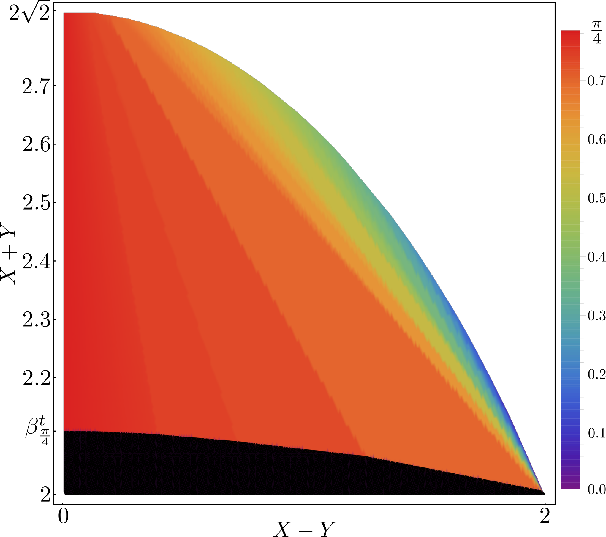
Self-testing of a maximally entangled two-qubit state from the CHSH score only depends on the value of $X+Y.$ Known bounds on ${\mathcal{F}}$ are reported as horizontal dashed lines in Fig. 3. We see from the figure self-testing based on the generalized CHSH scores outperforms CHSH for all pairs of values $(X,Y)$ where $X\neq Y$. In particular, self-testing based on generalized CHSH tests is possible even for CHSH scores below $\approx 2.05$ where no self-testing statement can be obtained from the CHSH score alone Valcarce2020. Note that, in extreme cases where $X<<Y$, self-testing is possible even for CHSH scores arbitrary close to (but strictly larger than) the local bound.

The most robust self-test of two-qubit maximally entangled states was obtained so far from the CHSH score $\beta=\langle A_{0}(B_{0}+B_{1})\rangle+\langle A_{1}(B_{0}-B_{1})\rangle.$ Despite several previous attempts, it was not clear how the knowledge of individual values $\langle A_{x}B_{y}\rangle$ can be used to improve the robustness of such a self-test. Here, we derive a self-testing strategy based on the knowledge of the two individual terms $X=\langle A_{0}(B_{0}+B_{1})\rangle$ and $Y=\langle A_{1}(B_{0}-B_{1})\rangle$ appearing in the CHSH score. We show in particular that such a strategy is equivalent to considering a family of generalized CHSH operators, and go on to present an explicit recipe for choosing the appropriate operator given observed values for the pair $(X,Y)$. We prove that using the available information of $X$ and $Y$ improves the bound on the fidelity with respect to CHSH for all pairs $(X,Y)$, except the one where $X=Y$. Furthermore, self-testing statements can be obtained for some pair $(X,Y)$ where the strategy based on the CHSH test fails. Our results facilitate the experimental implementation of any device-independent certification based on the self-test of maximally entangled two-qubit states.

We thank Jean-Daniel Bancal for fruitful discussions and comments. This work was supported by the Swiss National Science Foundation (SNSF) through the Grant PP00P2-179109 and the Region Ile-de-France in the framework of DIM SIRTEQ.

References

- (1) J. S. Bell, “On the einstein podolsky rosen paradox,” Physics Physique Fizika, vol. 1, pp. 195–200, Nov. 1964.
- (2) A. Montanaro and R. de Wolf Theory of Computing, vol. 1, no. 1, pp. 1–81, 2016.
- (3) I. Šupić and J. Bowles, “Self-testing of quantum systems: a review,” Quantum, vol. 4, p. 337, Sept. 2020.
- (4) J. F. Clauser, M. A. Horne, A. Shimony, and R. A. Holt, “Proposed experiment to test local hidden-variable theories,” Phys. Rev. Lett., vol. 23, pp. 880–884, Oct 1969.
- (5) N. Brunner, D. Cavalcanti, S. Pironio, V. Scarani, and S. Wehner, “Bell nonlocality,” Rev. Mod. Phys., vol. 86, pp. 419–478, Apr 2014.
- (6) S. Popescu and D. Rohrlich, “Which states violate bell’s inequality maximally?,” Physics Letters A, vol. 169, no. 6, pp. 411–414, 1992.
- (7) S. L. Braunstein, A. Mann, and M. Revzen, “Maximal violation of bell inequalities for mixed states,” Phys. Rev. Lett., vol. 68, pp. 3259–3261, Jun 1992.
- (8) D. Mayers and A. Yao, “Self testing quantum apparatus,” Quantum Info. Comput., vol. 4, pp. 273–286, July 2004.
- (9) C.-E. Bardyn, T. C. H. Liew, S. Massar, M. McKague, and V. Scarani, “Device-independent state estimation based on bell’s inequalities,” Physical Review A, vol. 80, dec 2009.
- (10) J.-D. Bancal, M. Navascués, V. Scarani, T. Vértesi, and T. H. Yang, “Physical characterization of quantum devices from nonlocal correlations,” Phys. Rev. A, vol. 91, p. 022115, Feb 2015.
- (11) T. H. Yang, T. Vértesi, J.-D. Bancal, V. Scarani, and M. Navascués, “Robust and versatile black-box certification of quantum devices,” Phys. Rev. Lett., vol. 113, p. 040401, Jul 2014.
- (12) J. Kaniewski, “Analytic and nearly optimal self-testing bounds for the clauser-horne-shimony-holt and mermin inequalities,” Physical Review Letters, vol. 117, Aug. 2016.
- (13) F. Magniez, D. Mayers, M. Mosca, and H. Ollivier, “Self-testing of quantum circuits,” in Automata, Languages and Programming (M. Bugliesi, B. Preneel, V. Sassone, and I. Wegener, eds.), (Berlin, Heidelberg), pp. 72–83, Springer Berlin Heidelberg, 2006.
- (14) P. Sekatski, J.-D. Bancal, S. Wagner, and N. Sangouard, “Certifying the building blocks of quantum computers from bell’s theorem,” Physical Review Letters, vol. 121, nov 2018.
- (15) S. Wagner, J.-D. Bancal, N. Sangouard, and P. Sekatski, “Device-independent characterization of quantum instruments,” Quantum, vol. 4, p. 243, Mar. 2020.
- (16) X. Valcarce, P. Sekatski, D. Orsucci, E. Oudot, J.-D. Bancal, and N. Sangouard, “What is the minimum CHSH score certifying that a state resembles the singlet?,” Quantum, vol. 4, p. 246, Mar. 2020.
- (17) J. Wang, S. Paesani, Y. Ding, R. Santagati, P. Skrzypczyk, A. Salavrakos, J. Tura, R. Augusiak, L. Mančinska, D. Bacco, D. Bonneau, J. W. Silverstone, Q. Gong, A. Acín, K. Rottwitt, L. K. Oxenløwe, J. L. O’Brien, A. Laing, and M. G. Thompson, “Multidimensional quantum entanglement with large-scale integrated optics,” Science, vol. 360, pp. 285–291, Mar. 2018.
- (18) K. T. Goh, C. Perumangatt, Z. X. Lee, A. Ling, and V. Scarani, “Experimental comparison of tomography and self-testing in certifying entanglement,” Phys. Rev. A, vol. 100, p. 022305, Aug 2019.
- (19) S. Gómez, A. Mattar, I. Machuca, E. S. Gómez, D. Cavalcanti, O. J. Farías, A. Acín, and G. Lima, “Experimental investigation of partially entangled states for device-independent randomness generation and self-testing protocols,” Phys. Rev. A, vol. 99, p. 032108, Mar 2019.
- (20) D. Orsucci, J.-D. Bancal, N. Sangouard, and P. Sekatski, “How post-selection affects device-independent claims under the fair sampling assumption,” Quantum, vol. 4, p. 238, Mar. 2020.
- (21) J.-D. Bancal, K. Redeker, P. Sekatski, W. Rosenfeld, and N. Sangouard, “Self-testing with finite statistics enabling the certification of a quantum network link,” Quantum, vol. 5, p. 401, Mar. 2021.
- (22) Y. Wang, X. Wu, and V. Scarani, “All the self-testings of the singlet for two binary measurements,” New Journal of Physics, vol. 18, p. 025021, Feb. 2016.
- (23) J.-D. Bancal, M. Navascués, V. Scarani, T. Vértesi, and T. H. Yang, “Physical characterization of quantum devices from nonlocal correlations,” Physical Review A, vol. 91, Feb 2015.
- (24) A. Acín, S. Massar, and S. Pironio, “Randomness versus nonlocality and entanglement,” Phys. Rev. Lett., vol. 108, p. 100402, Mar 2012.
- (25) E. Woodhead, A. Acín, and S. Pironio, “Device-independent quantum key distribution based on asymmetric chsh inequalities,” arXiv:2007.16146, 2020.
- (26) P. Sekatski, J. D. Bancal, X. Valcarce, E. Y. Z. Tan, R. Renner, and N. Sangouard, “Device-independent quantum key distribution from generalized chsh inequalities,” arXiv:2009.01784, 2020.
- (27) J. Kaniewski, “Self-testing of binary observables based on commutation,” Physical Review A, vol. 95, jun 2017.
- (28) J. Kaniewski, “Analytic and nearly optimal self-testing bounds for the clauser-horne-shimony-holt and mermin inequalities,” Phys. Rev. Lett., vol. 117, p. 070402, Aug 2016.
- (29) https://gitlab.com/plut0n/GenereralizedCHSH.
Appendix
A lower bound on the extractability can be obtained as the convex roof of the two-qubit optimisation defined in Eq. (11), over all generalized CHSH score . In this appendix, we give more details on how the optimization is performed.
For a given score , we minimize the fidelity with respect to over all two-qubit states and over all angles of measurement achieving a violation of at least Such an optimisation is formally expressed as