Canonical description of cosmological backreaction
Martin Bojowald** * e-mail address: bojowald@gravity.psu.edu and Ding Ding†† † e-mail address: dud79@psu.edu
Institute for Gravitation and the Cosmos,
The Pennsylvania State University,
104 Davey Lab, University Park, PA 16802, USA
Abstract
Canonical methods of quasiclassical dynamics make it possible to go beyond a strict background approximation for cosmological perturbations by including independent fields such as correlation degrees of freedom. New models are introduced and analyzed here for cosmological dynamics in the presence of quantum correlations between background and perturbations, as well as cross-correlations between different modes of a quantum field. Evolution equations for moments of a perturbation state reveal conditions required for inhomogeneity to build up out of an initial vacuum. A crucial role is played by quantum non-locality, formulated by canonical methods as an equivalent local theory with non-classical degrees of freedom given by moments of a quantum state.
1 Introduction
The backreaction problem in cosmology is concerned with the question of how an evolving or fluctuating quantum field in an expanding universe might affect the expansion rate of the background geometry on which it is defined. In the absence of a complete and consistent quantum theory of gravity or cosmology, the background is mainly treated as a classical system. The backreaction problem is therefore relevant not only for observational and conceptual questions in cosmology (see for instance [1, 2] for recent contributions), it also offers general lessons for the classical-quantum correspondence [3, 4, 5, 6, 7, 8, 9, 10, 11, 12, 13, 14, 15] and the validity of hybrid schemes in which only one part of an interacting system is quantum [16, 17, 18, 19]. In this paper, we apply recent advances in canonical descriptions of semiclassical expansions to a system that has been used recently as a cosmological model [20], to what turns out to be the leading semiclassical order of our systematic scheme.
We will use this systematic extension to construct new models for early-universe cosmology which may be interpreted as being of hybrid type. While we will not directly address the classical-to-quantum transition, we will be able to shed new light on the related homogeneity problem of inflationary structure formation [11], which states that it should be impossible for translation-invariant quantum evolution to generate inhomogeneity out of an initial homogeneous vacuum state. We will enter a crucial new ingredient into this discussion, given by quantum non-locality which is able to imply a gradual process of transfer of super-horizon inhomogeneity — suggested to occur generically according to the Belinskii–Khalatnikov–Lifshitz (BKL) scenario [21]) — down to smaller distance scales and eventually into the cosmological horizon. As an implication of quantum non-locality, this process may happen even in the quantization of a classical covariant theory. As we will observe for the first time in an application to quantum field theory, canonical moment methods give efficient access to spatial non-locality. (As has been known for some time, moment methods allow one to describe quantum non-locality in time by foregoing an adiabatic approximation of usual effective potentials.)
The classical Hamiltonian of the model used in [20] is given by
| (1) |
with two degrees of freedom and , where , and are positive constants. The degree of freedom remains completely classical in the original treatment and serves as a background which, while rolling down its linear potential , excites the oscillator given by via the interaction term . In [20], is quantized and its back-reaction effects on the roll-down rate of are studied. This dynamics could be considered a toy model representing the effects of particle creation on a classical background.
Here, we extend the model in a way that goes beyond a strict background treatment of . In the cosmological situation, the usual separation into background and perturbations exists only as an approximation of some inhomogeneous dynamics. Because both background and perturbation variables depend on the same fundamental degrees of freedom, given by the space-time metric and suitable matter fields, a separate quantization has a certain limited range of validity. Moreover, even classically the separation is not compatible with full general covariance but is maintained only by coordinate transformations that are small in the same sense in which inhomogeneity is considered a small perturbation on the background.
A complete treatment would have to be done within an elusive theory of quantum gravity, but while such a theory is still being constructed, some generic implications can be tested. In particular, if background and perturbations depend on the same fundamental fields, upon quantization there may well be correlations between them. Such correlations might even be required for general covariance to hold at the quantum level: Since a small coordinate change from to with an inhomogeneous , allowed at the perturbative level, maps a pure background variable such as the scale factor into an inhomogeneously perturbed quantity, , assuming vanishing quantum correlations between background and perturbations is likely too restrictive for a covariant quantum theory of the system.
The task then is to introduce correlation parameters between background and perturbations while maintaining a suitable level of tractability. We solve this problem here by utilizing a quasiclassical formulation of quantum dynamics [22, 23, 24, 25] which introduces (or derives) canonical variables for moments of a quantum state. (As we will also demonstrate, the constructions of [20] are equivalent to these quasiclassical methods.) Recent advances in [26, 27] have extended these methods from a single degree of freedom to a pair of coupled and possibly correlated degrees of freedom. This extension makes it possible to derive a systematic formulation of cosmological perturbations with background correlations.
In [28], a quantum-field version of the model of [20] was introduced and studied, concluding that it was not possible to solve the homogeneity problem. We describe and extend related models by applying systematic quasiclassical methods to a quantum field on a semiclassical background. Also here, we are able to introduce correlations between the field and the background. Importantly, we will also be able to reveal a new effect implied by the evolution of cross-correlations of different modes of a quantum field which can be used to address the homogeneity problem. In particular, we will observe that the usual assumption of an exactly homogeneous initial state is not always justified because super-Hubble inhomogeneity (as implied at early times by the BKL scenario) may trickle down to within the Hubble radius when quantum correlations are considered. We interpret this new effect as a consequence of quantum non-locality.
2 Canonical description of quantum dynamics
In order to facilitate the mathematical description of a quantum degree of freedom interacting with a classical variable, the construction presented in [20] uses a semiclassical approximation. Motivated by the well-known form of energy eigenstates of the harmonic oscillator, in particular of the Gaussian ground state, the authors observe that the first semiclassical correction of an oscillator can be described by doubling its degrees of freedom. That is, instead of a single variable , one may use a pair of degrees of freedom, and with momenta and , such that the quadratic potential is replaced by . The equations of motion are therefore given by
| (2) |
In addition, the angular momentum in the new -plane is constrained to be non-zero and equal to , restricting the allowed initial values. In particular, it is not possible for only one of the new variables to be non-zero, in which case we would have equivalence with the classical formulation.
In [20], this doubling of degrees of freedom of a semiclassical particle is obtained by including the variance as an independent degree of freedom, in addition to the expectation value of a basic variable such as (which vanishes in an energy eigenstate). The expectation value of in an uncorrelated Gaussian state with variance is given by
| (3) |
while the expectation value of (in any state) equals
| (4) |
The Gaussian expectation value of (1) in which only has been quantized is therefore
| (5) |
The contribution may be interpreted as a centrifugal potential of planar motion expressed in polar coordinates with radius , together with a spurious angle that does not appear in the potential of (5). Transforming to Cartesian coordinates implies the two degrees of freedom, and such that , with the condition that their angular momentum has to equal for in (5) to be the correct centrifugal potential. The harmonic potential is then turned into , which implies the equations of motion (2) for vanishing expectation value , as assumed in (2). To complete this construction, we also need a kinetic energy of the new variable or its Cartesian analogs and , which will be provided naturally by our more general treatment below.
For comparison, we briefly recall an alternative derivation of the equations of motion closer to the approach of [20]: The two degrees of freedom can be derived directly by introducing Heisenberg operators
| (6) | |||||
| (7) |
with the time-independent annihilation operator and a time-dependent complex function . Commutation relations then imply that
| (8) | |||||
| (9) |
where is the time-independent number operator. In the ground state, which we assume initially, where , we have
| (11) | |||||
| (12) |
valid at all times. Fluctuations therefore imply two dynamical real degrees of freedom. Moreover, the covariance (in the standard sense) equals
| (13) |
such that the uncertainty product
| (14) |
implies a constant in the Gaussian ground state. The specific angular momentum required by (5) is therefore closely related to the uncertainty relation.
We point out that the canonical formulation underlying this procedure has been known for some time, and has in fact been (re)discovered independently in various fields, including quantum field theory [22], quantum chaos [23] and quantum chemistry [24, 25]. Leading semiclassical corrections of a particle moving in one dimension with coordinate and momentum can be described by coupling the basic expectation values and to three additional variables, the quantum fuctuations and , as well as the covariance . It is useful to introduce a uniform notation that can easily be extended to higher moments, which we write, following [29, 30, 31], as
| (15) |
in completely symmetric, or Weyl ordering.
According to [29, 32], the expectation values and moments form a phase space equipped with a Poisson bracket defined by
| (16) |
and extended to moments by using the Leibniz rule. As a simple consequence, the Poisson bracket of basic expectation values equals the classical Poisson bracket, , and moments have zero Poisson brackets with basic expectation values. A closed-form expression exists for the bracket of two moments [29, 33], but it is rather complicated. In particular, it is not in canonical form.
For instance, for second-order moments, we have the brackets
| (17) |
With hindsight, the semiclassical formulation of [22, 23, 24, 25] can be interpreted as a mapping from the 3-dimensional Poisson manifold with brackets (17) to canonical, or Casimir–Darboux coordinates. Explicitly, defining the mapping from to by
| (18) |
or its inverse,
| (19) |
one can see that we have the canonical Poisson bracket , while .
These equations hold for all states. If we make the additional assumption that second-order moments provide a good approximation of quantum dynamics at least for some time, we may insert (19) in the expectation value of the harmonic Hamiltonian, taken in an arbitrary semiclassical state. We then obtain the effective Hamiltonian
| (20) |
still quantizing only . This Hamiltonian is equivalent to (5) if , the minimum value allowed by Heisenberg’s uncertainty relation. It is more general if is allowed to be greater than this value, in which case we are no longer restricted to Gaussian states. The derivation shows how the conserved quantity is related to the uncertainty relation as well as angular momentum in an effective description after transforming to Cartesian coordinates. Tranforming as the radial coordinate in an auxiliary plane (together with a spurious angle) to Cartesian coordinates on this plane, the centrifugal potential can be eliminated by doubling the fluctuation degree of freedom :
| (21) |
The kinetic energy of , or and , is automatically provided by (20). In general, angular momentum is bounded from below but not required to equal for generic states.
The effective Hamiltonian generates equations of motion for , and , as well as their momenta. Semiclassical aspects of quantum evolution can therefore be described by an enlarged phase space of classical type. Compared with the classical equations, solutions require additional initial values which partially encode properties of quantum states. The specification of an arbitrary state would require infinitely many parameters, for instance all moments required for the Hamburger problem that asks how a probability density can be reconstructed from all its moments. A semiclassical approximation replaces this infinite number with finitely many values, given by a minimum of three non-classical parameters , , and at leading semiclassical order.
A simple initial state, which may be Gaussian but would not be required to stay so in an interacting system, can be specified by the choice
| (22) |
The specific value chosen for mimics the ground state of a harmonic oscillator with frequency . We may leave the Casimir as a free parameter, which is restriced by the inequality but need not saturate it if the state is not required to be Gaussian. It would then be more difficult to find a specific wave function that belongs to these parameters, but semiclassical evolution based on the equations given here can be performed without problems. As shown in Fig. 1, the dynamics of the model applied in [20] to Gaussian states is indeed sensitive to the value of .

3 Correlations with the background
Having established the close relationship between [20] and canonical effective methods, we now use extensions of the latter to generalize the dynamics by including correlation degrees of freedom.
3.1 Motivation
In a traditional background treatment, the variable is treated completely classically, as in [20] and reviewed in the preceding section. However, if the system with Hamiltonian (1) is used as a toy model for particle production and backreaction in cosmology, the distinction between background degrees of freedom and perturbations is not as clear-cut because the model is then part of a generally covariant system subject to symmetries that act on matter fields as well as the space-time metric. A clear separation between background and perturbations as distinct degrees of freedom is usually available only in a fixed gauge, but not in a physical or gauge-invariant manner. For gauge-invariant properties, it is therefore of interest to go beyond a pure background treatment.
In particular, one commonly uses curvature perturbations or Mukhanov–Sasaki variables in order to put perturbative inhomogeneity into “gauge-invariant” form [34]. (In the present discussion, we may ignore the fact that these expressions are not fully gauge-invariant, but are so only with respect to a subset of all gauge transformations even in the linearized setting [35, 36].) These variables combine scalar modes of the metric with scalar fields. The former degrees of freedom form a single tensorial object together with the background metric, and therefore pure matter perturbations, distinct from the background, can be obtained only if a gauge is chosen in which the scalar modes of the metric vanish. In a gauge-invariant treatment, by contrast, it is not clear in which sense background and perturbations may be considered sufficiently independent to justify the assumption of vanishing correlations in a generic state upon quantization. (Thanks to general covariance, the quantum description of cosmological perturbations on an expanding background is not the same as quantum field theory on a curved background space-time, in which form it is often presented.)
In fact, the expressions for curvature perturbations in terms of metric and matter fields depend on the background scale fcator and the Hubble parameter. Background and perturbations are therefore not independent in a framework that somehow derives quantized perturbations from some fundamental, unperturbed quantum theory of gravity. Such a derivation would, of course, be challenging, but it suggests that background correlations should be relevant: Unless it can be shown that a quantum gravity could not possibly lead to quantum correlations between background and perturbations, it is not justified to assume that such correlations are absent or can be ignored. In this section, we derive a new theory of canonical effective equations with correlations, still applied to the toy Hamiltonian (1).
3.2 Canonical variables for second-order moments of two degrees of freedom
The technical task is then to generalize the simple mapping (19) to the moments of two classical degrees of freedom, with momentum and with momentum . To second order, each canonical pair has three individual moments, given by two fluctuations and a position-momentum covariance. These six individual moments are accompanied by four cross-covariances that contain one variable from each pair, such as . We therefore have a ten-dimensional Poisson manifold, which requires some work to put it into canonical form with Darboux coordinates and Casimir variables. This derivation has been completed only recently, in [26, 27], where explicit expressions for the ten second-order moments in terms of four pairs of Darboux coordinates — , , and — and two Casimir variables, and , have been provided.
The resulting expressions are rather complicated and, in contrast to (19), have momentum variances that cannot be put into a form suitable for canonical kinetic energies with constant coefficients. (A proof of this claim has been provided in [26].) Fortunately, as we will show here, they can be reduced in an approximate way that provides canonical kinetic energies and retains a single independent correlation parameter, .
We will quote here only the relevant moments. The new fluctuation parameters and as well as the correlation parameter are introduced by the equations
| (23) |
straightforwardly generalizing (19). Momentum variances also have a form similar to (19), given by
| (24) |
for the variance of . In contrast to (19), however, is not constant but rather depends on the canonical (Darboux) coordinates in the complicated form
| (25) |
where and are the two Casimir variables, and therefore conserved. A similar expression exists for .
This rather long expression has been derived in [27] from the conditions that the moments, expressed in canonical variables, (i) obey the required Poisson brackets and (ii) are represented in a one-to-one manner without loosing degrees of freedom in the canonical parameterization. This process, in particular the second condition, requires the inclusion of a canonical pair in (25) whose physical interpretation is not as clear as that of the fluctuation and correlation parameters , and together with their momenta.
A possible interpretation can be obtained from the fact that moments can be defined for any pure or mixed state. While the known meaning of , and as well as their momenta shows that they are free parameters even if one restricts oneself to pure states, there must be additional parameters in a parameterization of all states that determine how much they deviate from a pure state. The new canonical coordinates and , as well as , are candidates for such impurity parameters, a conjecture which has been tested with some success in a new canonical derivation of low-energy effective potentials given in [27].
3.3 Reduction of degrees of freedom
A minimal model that goes beyond the mapping for a single degree of freedom and retains a correlation parameter can be constructed as follows: We first assume that and are much smaller than and . The square root in (25) is then small, suppressing the dependence on via . The variable therefore need not be assumed small, and it may in fact grow because, according to the cross-term of the first square in , any effective Hamiltonian to which contributes in the kinetic energy, generates an equation of motion of the form where dots indicate terms independent of . It is therefore impossible for to be exactly zero if (a correlation parameter like ) is non-zero, while we need a non-zero in order to consistently ignore unless this variable is exactly zero. However, appears in a bounded function in (25) that is suppressed by a small square root if our assumption about and is satisfied, such that the dependence on can be ignored in this case. The interpretation of , and as impurity parameters suggests that our approximation should be valid whenever a state is close to being pure.
We then have the simplified expression
| (26) |
which, in a generalization of the momentum terms in (20), can be interpreted as (twice) the kinetic energy of a particle moving in three dimensions, expressed in spherical coordinates with a spurious degree of freedom . In contrast to the Cartesian version of (20), one of the angles, , now is physically meaningful. It is, in fact, the correlation parameter relevant for our present aims.
As shown by the last term in (26), the momentum of the spurious angle is constrained to equal the constant . If we include the second degree of freedom in the mapping, given by the background variable , it would have a similar kinetic energy with the same angle and its momentum . The two 3-dimensional systems would therefore be subject to constraints.
Here, we apply the 3-dimensional model only to the oscillating degree of freedom, , while the background degree of freedom is extended only by a fluctuation variable, , as in a mapping for a single degree of freedom. In this way, we are able to construct a minimal extension of the model by parameterizing the correlation variable, . For , we therefore have the kinetic contribution
| (27) |
as before, implying the contribution
| (28) |
to the effective potential in Cartesian coordinates, in the style of [20] but now applied also to the background.
For , we transform the kinetic energy implied by (26) to 3-dimensional Cartesian coordinates , such that
| (29) |
This variable contributes several terms to the effective potential:
| (30) |
where the last term comes from the correlation (23). The Hamiltonian is therefore
| (31) | |||||
For zero cross-correlations, we have and the Hamiltonian is reduced to a strict background model if we also set .
3.4 Diagonalization
The new effective Hamiltonian (31) can be interpreted as a system of four harmonic oscillators — , , and — with frequencies that depend on time through the background variable and its fluctuation parameter, . The term in (31) implies that and are not normal coordinates of the oscillator system.
We may attempt to (time-dependently) diagonalize this coupling between and the component of its fluctuation/correlation. In order for the diagonalization to be feasible, we assume that the typical time scale of evolution for and is much smaller than the time scale of and its fluctuations. We will then be able to treat the coefficients as approximately time-independent, allowing a straightforward diagonalization of the quadratic form.
Considering the entire Hamiltonian , the time scale for is of the order (noting that we set the mass to one and use natural units), while the time scale for is of the order , as will be confirmed in Fig. 5. Turning to and , we see that their time scales are roughly and which are typically very small because and grow large at late times. The hierarchy in time scales, along with the assumption , such that , justifies the following approximation.
We may rewrite the part of (31) as
| (32) |
where
| (33) |
Upon diagonalization we obtain the normal (angular) frequencies
| (34) | |||||
| (35) |
Since is the fluctuation of the classical degree of freedom, , we expect it to be much smaller than in magnitude. This result implies that the typical behavior of evolution of and can be described a fast, nearly harmonic oscillation with frequency , modulated by a slow oscillation with frequency . The introduction of the correlation parameter therefore gives rise to beat-like behavior, which is new and only present if we capture the effect of the background degree of freedom and its fluctuation using the 2-particle mapping.
The “normal coordinates” are given by
| (36) | |||||
| (37) |
where and are normalization constants. We see in Fig. 2 that the coefficients of and in the first line grow to be of similar magnitude but opposite signs, as a consequence of a decreasing such that the background degree of freedom is becoming more and more classical.

3.5 Dynamical implications
At the beginning of this section we showed that the semiclassical equations of motion for agree with those of [20], but only if as appropriate for a system in an initial vacuum state and only if a single degree of freedom, , is quantized. We can mimic the same initial conditon for the case where both degrees of freedom are quantized if we also impose , which we call the equivalence conditions. We also choose and other variables initially . The last two equalities for momenta are required by the interpretation of the Casimir variables identified with angular momentum.


Numerical similations with these conditions do not reveal any additional features as seen in Figs. 3 and 4. Therefore, the equivalence conditions turn the mapping for two degrees of freedom into a system equivalent with [20]. Even though we do introduce couplings of and to , the initial conditions and hence imply through out evolution, meaning that effectively couples only to , exactly as in the mapping for a single degree of freedom.


Interesting new effects are, however, obtained if the initial value of is not zero, such that we do not start in a vacuum state. Physically, it could be justified to use such initial values after a phase transition, where the inflaton field acquires a non-zero vacuum expectation value. For instance, using , Figs. 5 and 6 show that both and obtain new oscillatory features from the mapping for two degrees of freedom. In addition to fast oscillations, is also modulated by a slow-frequency oscillation. The -fluctuation, , also increases with time. Using (31), we can think of as a particle in a central-force problem, in which is subject to a central force that decreases with time due to the decrease of and . Since started off with a non-zero initial momentum due to the uncertainty relation, the particle (fluctuation) will eventually escape to a larger distance from the center.


The correlation of the two degrees of freedom is shown in Fig. 7. Two interesting features are the boundedness of in Fig. 8, and the upper bound of the background correlation between and for a given state in Fig. 7. The latter is explained by the interpretation of the correlation parameter as a spherical angle in an auxiliary space, implied by the appearance of (26) in the form of kinetic energy in spherical coordinates. The angular momentum in this auxiliary space is concerved and generically non-zero for a given initial state. For a non-zero value it is then impossible for the correlation angle to get arbitrarily close to the poles of the spherical system, such that keeps a certain distance from its general limiting values . This function equals the combination of moments plotted in Fig. 7, confirming the reduced upper bound for the given state implied by our initial values.
4 Field theory model
The formalism of [20] has also been applied to a quantum field back-reacting on a classical homogeneous background [37]. In this section, we will show how these methods are related to moments of a quantum field; see [38] for a general formulation of quantum fields by moments with a derivation of the Coleman–Weinberg potential [39]. The Coleman–Weinberg potential is conceptually related to the setting considered in [37] as it results from an expansion of a quantum field around a homogeneous background expectation value. The back-reaction equations of [37] can therefore be embedded in a canonical effective theory by a suitable extension of [38]. In particular, the equations correspond to a leading-order formulation of moment equations by canonical Darboux coordinates. In contrast to the previous section, however, a complete Darboux formulation of a quantum field is challenging because a single quantum field implies a multitude independent degrees of freedom, which are hard to describe by canonical variables for moments if all possible cross-correlations are included. Nevertheless, an embedding of [20] is feasible.
4.1 Modes on a compact homogeneous background
We consider a two-field model with a single spatial dimension, which will be reduced to a quantum field and a classical field . Both fields are scalar and real. Extending the interactions of (1), we introduce the classical action
| (38) |
with the mass of and a coupling constant that may be interpreted as providing a -dependent correction to the mass of . The field moves in a potential which, generically, may also include a mass term. As an extension of the preceding section, however, we will continue to assume that is linear in our numerical examples.
In the quantum-mechanical model of the previous section, back-reaction of on causes an exchange of energy: the quantum degree of freedom back-reacts on the classical one and saps its energy, causing to roll down more slowly on its linear potential. We expect similar transfer in energy in the field version, where the energy lost by the classical field excites particle production for the quantum field.
Using Legendre transformation we derive the Hamiltonian density
| (39) |
introducing
| (40) |
In order to facilitate an analysis of particle production, we should expand in Fourier modes with respect to a 1-dimensional, spatial wave number . The resulting system can then be interpreted as a background field, , coupled to a large number of oscillators with -dependent mass and frequency.
Fourier transforms of the basic canonical field are given by
| (41) | |||||
| (42) |
making time dependence implicit in this notation. The modes obey the reality conditions
| (43) |
Choosing opposite signs in the exponentials used to transform and , respectively, simplifies the canonical structure of modes. In particular, the calculation
| (44) |
implies that is canonically conjugate to .
Keeping the -Hamiltonian density unchanged, the Hamiltonian for Fourier modes is then given by
| (45) | |||||
with the non-local (in -space) contribution
| (46) |
In order to decouple different and obtain a local -Hamiltonian, we now assume that is homogeneous in , such that the -integration in results in a delta function that removes non-locality. Since depends on the background field according to (40), the background field is assumed to be spatially homogeneous from now on. It may, however, be time-dependent. With this assumption, the classical Hamiltonian
| (47) |
is local.
A final transformation introduces real fields in -space by splitting and into real and imaginary parts,
| (48) | |||||
| (49) |
Reality conditions imply that and are even functions while and are odd. Continuing the calculation in (44), we have
| (50) | |||||
The imaginary contribution vanishes because it integrates an odd function over the full real range of . The real contribution is even and can therefore be restricted to only positive , such that
| (51) |
If we restrict to positive , we therefore have the momenta and of and , respectively.
Our final expression for the classial Hamiltonian in terms of real modes is therefore
| (52) |
providing two harmonic oscillators per mode , each with a time-dependent frequency
| (53) |
that depends parameterically on the homogeneous background field . The -contribution to the Hamiltonian can directly be quantized to
| (54) |
Numerical simulations of our dynamics will be simpler if we replace the continuum of modes obtained so far with a discrete set by introducing periodic boundary conditions in space. We therefore assume that space is compactified to a circle with circumference . This finite size also makes the -Hamiltonian well-defined for a homogeneous . (The -Hamiltonian is described by a minisuperspace treatment, in which the averaging size would play an important role in quantum corrections if were quantized; see [40, 41]. Here, it is relevant for a consistent technical implementation of the background.) Our values of are then restricted to the discrete set
| (55) |
with a positive integer . The Hamiltonian for discrete modes can be derived by following the previous steps but replacing with , with , with .
We should also adjust the -Hamiltonian to its minisuperspace form. Starting with the original action (38) and introducing homogeneity such that , we see that the minisuperspace momentum is given by and depends on . The -Hamiltonian of the minisuperspace contribution therefore differs from (39) in that is replaced by . The Hamiltonian operator that combines a minisuperspace -contribution with a discrete set of -oscillators is then
| (56) |
Compared with a continuum of modes, we have to be careful with because the zero mode is real and therefore implies only one oscillator, .
4.2 Effective mode equations
As before, the Hamilton operator implies a quantum Hamiltonian evaluated in a generic state. We evaluate this Hamiltonian to second semiclassical order and, in a first step, ignore all cross-correlations. While this assumption constitutes a restriction on the class of states that can be studied with the model, we will show that it is self-consistent. The assumption relies on the condition that the -modes of are initially decoupled in terms of moments or cross-correlations, and remain so throughout evolution.
The modes are decoupled in our classical Hamiltonian. A sufficient condition for self-consistency of our assumption at the semiclassical level is then that all quadratic moments that involve different s remain zero if they vanish in an initial state. The relevant equations of motion are obtained from Poisson brackets, derived from (16), of the form where is a moments that appears in the quantum Hamiltonian .
For a second-order expansion of with an free of classical interactions between the modes, any is of the form of either or where each or refers to a single mode. In this case, we have
| (57) |
For a cross-covariance , we have . Therefore, any moment that may appear on the right-hand side of (57) with a non-zero coefficient is a cross-covariance. Analogous arguments hold for cross-covariances and of different modes. In general, therefore, calling the set of these mixed moments of -modes , Hamilton’s equations generated by using the Poisson bracket for moments are necessarily of the form for any , with moment-independent coefficients . Therefore, if all vanish initially, they remain zero at all times in this model.
Moments of the state, on which depends, can therefore self-consistently be expressed in canonical Darboux variables by using the same mapping (19) known for a single degree of freedom, but applied independently to each mode. This procedure leads to
| (58) | |||||
with canonical quantum degrees of freedom , , and such that
| (59) | |||||
| (60) |
All other variables in (58) are understood as expectation values of the basic mode, taken in the same state in which moments are computed.
Using canonical Poisson brackets for all variables in (58) except for the constant and , we derive second-order equations of motion
| (61) | |||||
| (62) | |||||
| (63) | |||||
| (64) |
In the first line, we have used the specific frequency (40).


Equations (61)–(64) are coupled and hard to solve analytically, but numerical solutions can be obtained for specific initial values. We assume a background potential in what follows and choose the moments of each -mode to correspond to the Gaussian ground state inititally, with frequency . In particular, for all . The initial value for that appears in the frequencies is assumed to vanish, as are all other dynamical variables.
Figures 9 and 10 show the background evolution and the magnitude of back-reaction, using a momentum cutoff of and the parameters , , . Except for the momentum cutoff, these parameters match the ones used in Figures 3–5 of [37]. Their momentum cutoff is while for us it is . There are also differences in the treatment of quantum fields, which explains why numerical evolutions in these two approaches do not align precisely in quantitative terms. In addition, [37] also considers non-linear potentials in detail, from which we refrain here in a first analysis. For smaller , it takes longer and longer for to turn around as a consequence of back-reaction. The longer phase of increasing makes it difficult to resolve the turn-around numerically for very small , but the general trend of a delayed turn-around is illustrated in Figure 11.
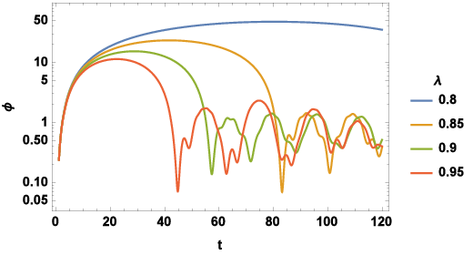
Nevertheless, our numerical results are qualitatively comparable with those of [37]. The models are not identical because we evolve mode equations on a compact space, while [37] considers a lattice approximation to evolve spatial fields. The homogeneity assumption on the background is shared by both approaches, except for a small excursion into inhomogeneous backgrounds at the end of [37]. The underlying equations are also identical because equation (2) of [37], given by
| (65) |
is equivalent to our mode equations for a homogeneous background. In particular, our mode equations correspond to the Klein–Gordon equation
| (66) |
with a source term for back-reaction. This equation is the same as equation (9) of [37] for a homogeneous .
4.3 Interactions and correlations with the background
The homogeneity problem in inflationary cosmology is concerned with the question of how it can be possible for inhomogeneity to develop out of an initial homogeneous vacuum state, subject to translation invariant dynamics that should not break this symmetry. (See for instance [3, 4, 11, 13, 14, 15].) Effective equations for moments of a quantum field or their canonical variables can be a powerful tool to determine conditions under which inhomogeneity may build up. Similar considerations show that quantum correlations with the background may be relevant in certain situations. Specific details of such back-reaction effects may also be relevant for observational questions in cosmological eras at later times [42, 43, 1, 2].
4.3.1 Inhomogeneity from a back-reacting vacuum
We assume that our initial state for quantum field and classical background is spatially homogeneous. Suitable conditions on initial moments are expressed in our notation as
| (67) | |||
| (68) | |||
| (69) |
where the sum excludes , or alternatively for all .
At this point it is important to note that choosing a specific initial state poses a condition on initial values for evolution, but it should not restrict the general dynamics of a background interacting with a quantum field. Therefore, in order to consider the possibility of background inhomogeneity being generated, the Hamiltonian should contain kinetic, potential, and interaction terms for a generic inhomogeneous background field , including its momentum in a canonical formulation. If we were to represent the background as a homogeneous minisuperspace model as in (56), background inhomogeneity would be excluded by fiat. In order to see how inhomogeneity may be generated, we should start with the more general Hamiltonian (54) with a field Hamiltonian density and study the evolution it generates starting with symmetric initial conditions (67) for a homogeneous initial state. The expectation value in a generic field state is a suitable effective Hamiltonian for this analysis. Here we encounter the important distinction between quantum field theory on a homogeneous background, which would be described by our minisuperspace background, and a more complete treatment of an interacting field and background.
A key contribution in this Hamiltonian that does not appear in the minisuperspace version is the interaction term
| (70) |
Using symmetric initial conditions, the momentum conjugate to evolves according to
| (71) | |||||
keeping only terms that have a chance of being non-zero. Given our initial conditions, the last integrand is initially non-zero if and only if , and therefore does not vanish. (Physically, cannot be perfectly homogeneous due to the uncertainty relation, such that .)
Even for an initially homogeneous , the coupling implies that the background field , seen as a harmonic oscillator, may have a position-dependent frequency . If the initial state is completely homogeneous, the frequency is homogeneous and no background inhomogeneity is generated, in accordance with the expectation based on translation-invariant dynamics. However, this condition on the initial state is rather strong because it imposes homogeneity in all of space at an initial time, potentially far beyond the Hubble radius that would be accessible by causality. This assumption is not consistent with the generic behavior of space-time expected near a spacelike singularity such as the big bang according to the Belinskii–Khalatnikov–Lifshitz (BKL) scenario [21].
There should therefore be a certain mode number at which strict homogeneity breaks down. On these scales, the background field oscillates differently at different places and cannot stay homogeneous. One might expect that such large-scale inhomogeneity far outside the Hubble radius may not be relevant, but we will now show that moment dynamics of the field implies that large-scale inhomogeneity eventually trickles down to smaller scales, at which the background inhomogeneity it generates will be relevant.
It is perhaps surprising that moment terms from a quantum field allow inhomogeneity to travel from large scales into a cosmological horizon. Our results show that this is indeed possible even in a quantization of a classically causal theory because we start with standard covariant action of a scalar field. In fact, as our derivation shows, inhomogeneity builds up on smaller scales through a gradual process of growing cross-correlations, rather than direct propagation that would be impossible in a causal theory.
A useful interpretation of the gradual process we derived is as an effect of quantum non-locality. Moment methods make it possible to formulate effective field theories without performing a derivative expansion. This feature has been know for some time in an application to quantum mechanics, such as in quantum chemistry [25] where they give access to non-adiabatic reaction dynamics. In [29, 32, 44], it was shown explicitly that a combination of moment methods with an adiabatic approximation yields results equivalent to the low-energy effective potential [45] or higher-derivative corrections. Similarly, in an application to scalar field theories, a combination of moment methods and an adiabatic approximation [38] allows one to rederive the Coleman–Weinberg potential [39]. In the present paper, however, we have applied moment methods to quantum field theories without using an adiabatic approximation.
Instead of higher-derivative corrections, our effective Hamiltonians implement quantum corrections through coupling terms to non-classical fields as new independent degrees of freedom, such as the modes and in canonical terms or directly in terms of moments. It is possible to interpret such an extended field theory as a local formulation of a non-local theory without extra degrees of freedom: If one were able to solve equations of motion for the new fields as functions of the classical fields and to insert them in the extended Hamiltonian, local terms would be replaced by integrals representing solutions of partial differential equations. It would be cumbersome to do so in practice, and it is in fact easier to analyze the local extended system. Nevertheless, the argument demonstrates that the build-up of inhomogeneity derived here is a consequence of quantum non-locality, a crucial new ingredient in early-universe cosmological models.
4.3.2 Field correlations
If inhomogeneity is included in the background Hamiltonian and its coupling terms, new interaction channels open up for oscillator moments that are not contained in models with a strictly homogeneous background. To simplify the discussion, we assume now that the background is homogeneous up to adding a single mode, . The interaction term then depends on the -modes through the terms and obtained directly from . The non-local expression (46) is then again local, but with additional interaction terms:
| (72) | |||||
There are therefore interactions between neighboring modes over distances and . Any interaction potential of the form with some constant implies evolving cross-correlations, which we express here directly in terms of moments without a canonical parameterization. A second-order effective Hamiltonian contains the moments . Since the variances cannot be zero as per uncertainty relations, the effective Hamiltonian implies non-zero time derivatives of moments of the form , using the Poisson bracket
| (73) |
Similarly, has a non-zero time derivative because
| (74) |
Once have evolved to non-zero values (assuming they start at zero for an uncorrelated initial state), the time derivatives of will be non-zero, using
| (75) |
and a contribution from the kinetic energy to the effective Hamiltonian.
The state therefore evolves to non-zero correlations at a -space distance . Then, we have non-zero time derivatives of because of a non-zero
| (76) |
where is again a term in the effective potential. Non-zero then imply non-zero time derivatives of through the kinetic terms of the effective Hamiltonian. Iteration shows that shorter-range correlations of increasing in develop over time, provided the background is not exactly homogeneous.
Turning now to evolution equations for moments of background modes of inhomogeneity, the middle term in (72), inserted in an effective Hamiltonian, shows that any momentum of a -mode, such that has developed a non-zero value, has a non-zero time derivative. Even if the initial was zero, therefore, background inhomogeneity develops in a large number of modes (all integer multiples of ) provided there was some initial inhomogeneity in just one mode, . If the wave length corresponding to the initial is super-Hubble, as suggested by the BKL scenario, correlations in and then inhomogeneity in trickles down to smaller wave lengths (larger ) that eventually enter the Hubble radius and become relevant for the history of our visible universe. These results provide a consistent picture of the generation of background inhomogeneity in cosmology. (We note that the situation in cosmology is different from quantum phase transitions in which structure may also form, as studied for instance in [46]. In the latter case, an infinite-volume limit is required for a mathematical description of the phase transition, and homogeneity of the pre-transition state may be assumed even in the limit. In cosmology, the BKL scenario prevents one from making the same assumption.)
4.3.3 Background correlations in quantum field theories
In addition to indirect effects of field correlations on the background dynamics as just discussed, a general quantum description of background and field modes may contain direct quantum correlations between the background and the field. Such correlations are also excluded by fiat in a strict background treatment, but they can be included in an extended model using our new methods. We briefly present here such models, but for now refrain from analyzing them.
The restricted second-order Hamiltonian (31) suggests an extension of the background-field model to multiple canonical fields for background and oscillators. Some of the new fields represent quantum degrees of freedom for fluctuations, as before, and others cross-correlations between background and oscillator fields. Promoting all variables in (31) to fields, we obtain the Hamiltonian density
| (77) | |||||
with five new fields, , , , and , and the same as before. The field describes background correlations.
For a homogeneous background , a mode expansion is still possible, resulting in local, decoupled Hamiltonians for the modes. The potential
| (78) | |||||
then implies three different frequencies,
| (79) |
for and
| (80) |
for as well as , and a rotation coefficient
| (81) |
between and . As before, beat-like effects are expected by mode mixing.
If the background is homogeneous, a single correlation field is sufficient to extend the model to background correlations. In addition, there may be correlations between different modes of the field , which at present is hard to describe in canonical quasiclassical form because a complete set of Casimir–Darboux for a quantum field remains unknown. Instead, one may construct a completely correlated background-field model by keeping the background correlation field in canonical quasiclassical form, while fully quantizing the field or its modes as before. In (77), , and as well as their momenta would then be replaced by a single field operator , while remains a single field of classical type. In this formulation, hybrid methods of classical-quantum dynamics, such as [16, 17, 18, 19], would find a useful place in cosmology.
5 Conclusions
We have significantly extended a back-reaction model considered in [20] in order to study implications of backreaction and the build-up of inhomogeneity in cosmological evolution. To this end, we first showed that the formalism of [20] is equivalent to a special case of non-adiabatic semiclassical approximations obtained from the dynamics of moments parameterizing an evolving state. The restricted nature of the formalism developed in [20] implies that there are key distinctions between the two approaches that provide different advantages, depending on what physical system is being studied.
The formalism of [20] is efficient in tackling quadratic Hamiltonians and Gaussian approximations. For anharmonic systems, its approximate equations of motion remain quite simple, but there is no self-consistent way to determine whether the approximation is reliable. This shortcoming is related to a lack of physical interpretation of the degrees of freedom, and , used in [20] to describe quantum variables. The derivation of how these variables appear in a Hamiltonian or in equations of motion requires a wave function , usually assumed Gaussian, but the reduction of infinitely many quantum degrees of freedom implicitly described by the functional dependence of to just two relevant ones is not systematic. In cases in which no suitable wave function is known, for instance in situations of particle creation that lead one away from a vacuum state, the predictability of the formalism remains unclear. No recipe for going beyond leading order (in some kind of loop expansion) has been developed.
Our embedding of the formalism of [20] in the systematic framework of canonical effective theory helps to make the approximations much more systematic. The quantum degrees of freedom are now physically interpreted as moments of a state, not just in Gaussian or near-Gaussian situations. There is a clear extension to higher orders of moments, mimicking the loop expansion of interacting theories. To low orders, as we have shown, explicit canonical realizations are available and can be used to extend the model of [20] to correlation degrees of freedom. As we have argued, these degrees of freedom are crucial for cosmological back-reaction in which no sharp physical separation between background and perturbations exists, owing to general covariance. Correlation degrees of freedom are then seen to give rise to new beat-like effects that may be relevant in particle production.
Extended models also show how background inhomogeneity may be generated out of a symmetric sub-horizon initial state, and what role may be played by various forms of quantum correlations. We recognized that the extension to moments as independent degrees of freedom can be interpreted as a local formulation of quantum non-locality, which in this form has not been considered before in early-universe models. By an explicit calculation of equations of motion for moments we showed that quantum non-locality implies a gradual build-up of inhomogeneity within a cosmological horizon, even if the initial sub-horizon state is completely homogeneous but inhomogeneity exists on much larger scales. This build-up of inhomogeneity is a consequence of quantum non-locality and does not violate causal propagation. The new effect is therefore able to solve the homogeneity problem of inflationary structure formation.
Acknowledgements
This work was supported in part by NSF grant PHY-1912168. We thank Mainak Mukhopadhyay and Tanmay Vachaspati for discussions and useful suggestions.
References
- [1] L. Perreault-Levasseur and E. McDonough, Backreaction and Stochastic Effects in Single Field Inflation, Phys. Rev. D 91 (2015) 063513, [arXiv:1409.7399]
- [2] C. Armendariz-Picón, On the Expected Backreaction During Preheating, JCAP 05 (2020) 035, [arXiv:2003.01542]
- [3] J. J. Halliwell, Correlations in the wave function of the Universe, Phys. Rev. D 36 (1987) 3626–3640
- [4] J. J. Halliwell, Decoherence in quantum cosmology, Phys. Rev. D 39 2912
- [5] D. Polarski and A. A. Starobinsky, Semiclassicality and Decoherence of Cosmological Perturbations, Class. Quant. Grav. 13 (1996) 377–392, [gr-qc/9504030]
- [6] J. Lesgourgues, D. Polarski, and A. A. Starobinsky, Quantum-to-classical Transition of Cosmological Perturbations for Non-vacuum Initial States, Nucl. Phys. B 497 (1997) 479–510, [gr-qc/9611019]
- [7] C. Kiefer, D. Polarski, and A. A. Starobinsky, Quantum-to-classical transition for fluctuations in the early Universe, Int. J. Mod. Phys. D 7 (1998) 455–462, [gr-qc/9802003]
- [8] C. Kiefer and D. Polarski, Emergence of classicality for primordial fluctuations: Concepts and analogies, Annalen Phys. 7 (1998) 137–158, [gr-qc/9805014]
- [9] A. O. Barvinsky, A. Yu. Kamenshchik, and C. Kiefer, Effective action and decoherence by fermions in quantum cosmology, Nucl. Phys. B 552 (1999) 420–444, [gr-qc/9901055]
- [10] A. O. Barvinsky, A. Yu. Kamenshchik, C. Kiefer, and I. V. Mishakov, Decoherence in quantum cosmology at the onset of inflation, Nucl. Phys. B 551 (1999) 374–396
- [11] A. Perez, H. Sahlmann, and D. Sudarsky, On the quantum origin of the seeds of cosmic structure, Class. Quantum Grav. 23 (2006) 2317–2354, [gr-qc/0508100]
- [12] C. Kiefer, I. Lohmar, D. Polarski, and A. A. Starobinsky, Pointer states for primordial fluctuations in inflationary cosmology, Class. Quantum Grav. 24 (2007) 1699–1718, [astro-ph/0610700]
- [13] A. De Unánue and D. Sudarsky, Phenomenological analysis of quantum collapse as source of the seeds of cosmic structure, Phys. Rev. D 78 (2008) 043510, [arXiv:0801.4702]
- [14] G. León and D. Sudarsky, The slow roll condition and the amplitude of the primordial spectrum of cosmic fluctuations: Contrasts and similarities of standard account and the “collapse scheme”, Class. Quant. Grav. 27 (2010) 225017, [arXiv:1003.5950]
- [15] J. Berjon, E. Okon, and D. Sudarsky, Debunking prevailing explanations for the emergence of classicality in cosmology, [arXiv:2009.09999]
- [16] E. C. G. Sudarshan, Interaction between classical and quantum systems and the measurement of quantum observables, Pramana 6 (1976) 117
- [17] R. Kapral, Progress in the theory of mixed quantum–classical dynamics, Ann. Rev. Phys. Chem. 57 (2006) 129–57
- [18] D. I. Bondar, F. Gay-Balmaz, and C. Tronci, Koopman wavefunctions and quantum–classical correlation dynamics, Proc. R. Soc. A 475 (2019) 20180879, [arXiv:1802.04787]
- [19] F. Gay-Balmaz and C. Tronci, Madelung transform and probability densities in hybrid classical-quantum dynamics, Nonlinearity 33 (2020) 5383, [arXiv:1907.06624]
- [20] T. Vachaspati and G. Zahariade, A Classical-Quantum Correspondence and Backreaction, Phys. Rev. D 98 (2018) 065002, [arXiv:1806.05196]
- [21] V. A. Belinskii, I. M. Khalatnikov, and E. M. Lifschitz, A general solution of the Einstein equations with a time singularity, Adv. Phys. 31 (1982) 639–667
- [22] R. Jackiw and A. Kerman, Time Dependent Variational Principle And The Effective Action, Phys. Lett. A 71 (1979) 158–162
- [23] R. A. Jalabert and H. M. Pastawski, Environment-independent decoherence rate in classically chaotic systems, Phys. Rev. Lett. 86 (2001) 2490–2493
- [24] F. Arickx, J. Broeckhove, W. Coene, and P. van Leuven, Gaussian Wave-packet Dynamics, Int. J. Quant. Chem.: Quant. Chem. Symp. 20 (1986) 471–481
- [25] O. Prezhdo, Quantized Hamiltonian Dynamics, Theor. Chem. Acc. 116 (2006) 206
- [26] B. Baytaş, M. Bojowald, and S. Crowe, Faithful realizations of semiclassical truncations, Ann. Phys. 420 (2020) 168247, [arXiv:1810.12127]
- [27] B. Baytaş, M. Bojowald, and S. Crowe, Effective potentials from canonical realizations of semiclassical truncations, Phys. Rev. A 99 (2019) 042114, [arXiv:1811.00505]
- [28] T. Vachaspati and G. Zahariade, Classical-Quantum Correspondence for Fields, JCAP 09 (2019) 015, [arXiv:1807.10282]
- [29] M. Bojowald and A. Skirzewski, Effective Equations of Motion for Quantum Systems, Rev. Math. Phys. 18 (2006) 713–745, [math-ph/0511043]
- [30] M. Bojowald and A. Tsobanjan, Effective constraints for relativistic quantum systems, Phys. Rev. D 80 (2009) 125008, [arXiv:0906.1772]
- [31] A. Tsobanjan, Semiclassical states on Lie algebras, J. Math. Phys. 56 (2015) 033501, [arXiv:1410.0704]
- [32] M. Bojowald and A. Skirzewski, Quantum Gravity and Higher Curvature Actions, Int. J. Geom. Meth. Mod. Phys. 4 (2007) 25–52, [hep-th/0606232], Proceedings of “Current Mathematical Topics in Gravitation and Cosmology” (42nd Karpacz Winter School of Theoretical Physics), Ed. Borowiec, A. and Francaviglia, M.
- [33] M. Bojowald, D. Brizuela, H. H. Hernandez, M. J. Koop, and H. A. Morales-Técotl, High-order quantum back-reaction and quantum cosmology with a positive cosmological constant, Phys. Rev. D 84 (2011) 043514, [arXiv:1011.3022]
- [34] V. F. Mukhanov, H. A. Feldman, and R. H. Brandenberger, Theory of cosmological perturbations, Phys. Rept. 215 (1992) 203–333
- [35] J. M. Stewart, Perturbations of Friedmann–Robertson–Walker cosmological models, Class. Quantum Grav. 7 (1990) 1169–1180
- [36] M. Bojowald, Non-covariance of the dressed-metric approach in loop quantum cosmology, Phys. Rev. D 102 (2020) 023532, [arXiv:2002.04986]
- [37] M. Mukhopadhyay and T. Vachaspati, Rolling with quantum fields, [arXiv:1907.03762]
- [38] M. Bojowald and S. Brahma, Canonical derivation of effective potentials (2014), [arXiv:1411.3636]
- [39] S. Coleman and E. Weinberg, Radiative corrections as the origin of spontaneous symmetry breaking, Phys. Rev. D 7 (1973) 1888–1910
- [40] M. Bojowald and S. Brahma, Minisuperspace models as infrared contributions, Phys. Rev. D 92 (2015) 065002, [arXiv:1509.00640]
- [41] M. Bojowald, The BKL scenario, infrared renormalization, and quantum cosmology, JCAP 01 (2019) 026, [arXiv:1810.00238]
- [42] R. H. Brandenberger, Back Reaction of Cosmological Perturbations and the Cosmological Constant Problem, [hep-th/0210165]
- [43] R. H. Brandenberger, L. L. Graef, G. Marozzi, and G. P. Vacca, Back-Reaction of Super-Hubble Cosmological Perturbations Beyond Perturbation Theory, Phys. Rev. D 98 (2018) 103523, [arXiv:1807.07494]
- [44] M. Bojowald, S. Brahma, and E. Nelson, Higher time derivatives in effective equations of canonical quantum systems, Phys. Rev. D 86 (2012) 105004, [arXiv:1208.1242]
- [45] F. Cametti, G. Jona-Lasinio, C. Presilla, and F. Toninelli, Comparison between quantum and classical dynamics in the effective action formalism, In Proceedings of the International School of Physics “Enrico Fermi”, Course CXLIII, pages 431–448, Amsterdam, 2000. IOS Press, [quant-ph/9910065]
- [46] M. Mukhopadhyay, T. Vachaspati, and G. Zahariade, Quantum Formation of Topological Defects, Phys. Rev. D 102 (2020) 116002, [arXiv:2009.11480]