Fast Solver for Quasi-Periodic 2D-Helmholtz Scattering in Layered MediaThanks: This work was partially funded by Fondecyt Regular 1171491 and by grants Conicyt-PFCHA/Doctorado Nacional/2017-21171791 and 2017-21171479.
Abstract
We present a fast spectral Galerkin scheme for the discretization of boundary integral equations arising from two-dimensional Helmholtz transmission problems in multi-layered periodic structures or gratings. Employing suitably parametrized Fourier basis and excluding Rayleigh-Wood anomalies, we rigorously establish the well-posedness of both continuous and discrete problems, and prove super-algebraic error convergence rates for the proposed scheme. Through several numerical examples, we confirm our findings and show performances competitive to those attained via Nyström methods.
1 Introduction
A vast number of scientific and engineering applications rely on harnessing acoustic and electromagnetic wave diffraction by periodic and/or multilayered domains. Current highly demanding operation conditions for such devices require solving thousands of specific settings for design optimization or the quantification of shape or parameter uncertainties in the relevant quantities of interest, challenging the scientific computing community to continuously develop ever more efficient, fast and robust solvers (cf. [8, 18, 31, 40, 39] and references therein). Assuming impinging time-harmonic plane waves, scattered and transmitted fields have been solved by a myriad of mathematical formulations and associated solution schemes. These range from volume variational formulations to various boundary integral representations and equations (cf. [2, 4, 9, 11, 21, 33]), pure or coupled implementations of finite and boundary element methods (cf. [3, 4, 22, 34, 40] or [36, Chapter 5]) and Nyström methods [15, 17, 19, 24, 30].
In this work, we build upon our theoretical review given in [5] and present a spectral Galerkin method for solving second-kind direct boundary integral equations (BIEs) for the Helmholtz transmission problem for two-dimensional, periodic multi-layered gratings with smooth interfaces. Contrary to the low-order local basis functions used in the standard boundary element method, spectral bases are composed of high-order polynomials whose support lie on the whole scatterer boundary or on large portions of it. Successfully employed on two- and three-dimensional scattering problems [26, 25, 23], the main advantage of a spectral discretization is the ability to converge at a super-algebraic rate whenever solutions are smooth enough. Hence, our proposed method can in practice compete with Nyström methods while simultaneously inheriting all of the theoretical aspects of classical Galerkin methods.
In two dimensions, spectral methods are closely related to the theory of periodic pseudo-differential operators [37], since the discretization through spectral elements can be interpreted as a truncation of the associated Fourier series where the action of the operators is well understood. We show that wave scattering by periodic domains is closely connected to the bounded domain case, making it possible to reuse almost all the pseudo-differential operator theory for our analysis. Key to our analysis are the results in [34, 41, 22] regarding the unique solvability and eigenvalues of the associated volume problem. From here, we deduce that our BIE is uniquely solvable except at a countable set of wavenumbers composed of Rayleigh-Wood frequencies—wavenumbers for which the sum defining the quasi-periodic Green’s function is not convergent—and of eigenvalues of the Helmholtz transmission problem. Mindless of the several remedies developed to tackle Rayleigh-Wood anomalies through BIEs [19, 13, 16, 14], we choose to avoid them as they are not captured by our previous analysis in [5].
Our discretization method employs a quasi-periodic basis so that techniques forcing the quasi-periodicity of the discrete solutions are not necessary (cf. [24, 46]). Instead, an accurate approximation of the quasi-periodic Green’s function is required in order to extract its Fourier coefficients through the fast Fourier transform (FFT). Moreover, we prove that the chosen discretization basis enjoys a super-algebraic convergence rate on the degrees of freedom, which we then confirm through numerical experiments. In [35], a similar quasi-periodic exponential basis was employed to approximate solutions of a volume integral formulation.
The article is structured as follows. Section 2 presents the notation used throughout as well as the required quasi-periodic Sobolev spaces setting following [5]. In Section 3 we state the Helmholtz transmission problem for a multi-layered grating and study its solvability. Section 4 is concerned with the properties of quasi-periodic boundary integral operators (BIOs) along with an existence and uniqueness result for our BIEs. Section 5 provides rigorous error convergence rates of the spectral method and briefly describes the numerical algorithm used to compute the matrix entries associated with each integral operator. Numerical results are discussed in Section 6, followed by concluding remarks on Section 7.
2 Notation and Functional Space Setting
2.1 General Notation
We denote the imaginary unit . Boldface symbols will denote vectorial quantities and will use greek and roman letters for data over boundaries and volume, respectively. Canonical vectors in are denoted respectively. Also, we make use of the symbols , and to avoid specifying constants irrelevant for the corresponding analysis.
Let be a given Banach space. We shall denote its norm as and its dual space by (set of antilinear functionals over ) with dual product denoted by . If is a Hilbert space, the inner product between two of its elements, and , is denoted as . Moreover, if is a Hilbert space over the complex field, the inner product will be understood in the anti-linear sense.
For an open domain , its boundary shall be denoted as . Moreover, for any such that , we introduce the closure of relative to as and the boundary of relative to as .
For , we denote by the set of scalar functions over with complex values and continuous derivatives up to order . refers to the space of functions with infinite continuous derivatives over . We shall also make use of the following subset of :
The space of -integrable functions (for ) with complex values over is denoted as .
We say that a one-dimensional Jordan curve is of class , for , if it may be parametrized by a function which has Lipschitz-continuous derivatives and a non-vanishing tangential vector. The first derivative of the parametrization is denoted as . Moreover, we say is of class if it is of class for every (we will also use the notation to refer to the same class).
Throughout the following sections, we will consider periodic geometries along with a fixed period of . Moreover, we say that a continuous function is a -quasi-periodic function if,
where the quasi-periodic shift is always assumed to be in . Finally, we define the canonic periodic cell on as .
2.2 Quasi-periodic Sobolev Spaces
We denote by the space of -quasi-periodic functions in that vanish for large , and denote by the space of -quasi-periodic distributions, which can be seen as the dual space of (cf. [5, Proposition 2.4]). For as before, we introduce the space of restrictions to of elements in . Moreover, for any open domain we define as the set of elements of with compact support on and as the space of elements of restricted to . In what follows, for all we define .
Proposition 2.1 (Proposition 2.6 in [5]).
Every can be represented as a Fourier series, i.e.
so that . On the other hand, every element can be identified with a formal Fourier series given by
where for all and .
Let . We define the -quasi-periodic Sobolev space of order on as follows,
wherein is the Fourier transform (in distributional sense [42, Section 2.4]) of , defined as in Proposition 2.1. Additionally, we introduce the common notation and note that, as in the standard case, is a Hilbert space [5, Proposition 2.8]. Furthermore, for an open proper subset of , we define as the Hilbert space of restrictions to of elements of (see [5, Section 2] and [32, Chapter 3.6]). Finally, local Sobolev spaces on are defined as
2.3 Quasi-periodic Sobolev Spaces on Boundaries and Traces
We begin by considering spaces of periodic functions over . As in [28, Definition 8.1], [37, Section 5.3], we define Sobolev spaces on of order as follows,
where are the Fourier coefficients of . Quasi-periodic spaces of order over are defined from straightforwardly, i.e.,
Both and are Hilbert spaces, as are their respective dual spaces, denoted respectively and (see [28, Theorem 8.10] and [5, Theorem 2.20]). Moreover, for , the inner product and norm of are given by:
wherein, for positive , we define
and the product is extended through duality to negative (cf. [5, Theorems 2.16 and 2.20]).
We continue by considering boundaries which are constructed as the single period of a periodic Jordan curve of class . Let be one of such curves and let be a parametrization of . Then, for any , we define the -quasi-periodic Sobolev space of order on as
We define as the completion of under the norm given by
Norms and inner products for these spaces are given through their respective pullbacks to and . Moreover, is identified with the dual space of [5, Theorem 2.26] where the duality is given by the extension of the following anti-liner form:
| (1) |
We also define the following space of smooth functions over ,
which is dense on for any . Finally, we introduce trace operators acting on quasi-periodic Sobolev spaces. Let be a proper open subset of such that , we define the following operators for :
that extend the notion of the restriction operator to quasi-periodic Sobolev spaces [5, Theorem 2.29]. In this context, and are, respectively, the interior and exterior Dirichlet traces. Analogously, for , we denote the interior and exterior Neumann traces on as
extending the normal derivative , where is—for both traces—the unitary normal exterior to . Moreover, introducing the subspace of elements of with integrable Laplacian,
the Neumann trace may be extended as
through integration by parts (cf. [5, Section 2]). All the previous results concerning trace operators follow analogously (with obvious modifications) for both local spaces—in the case that is unbounded—and if is the bounded space between two non-intersecting periodic curves and . Finally, we denote the following vector operators
as the interior, exterior and jump trace vectors on , respectively.
3 Helmholtz problem in periodic layered media
3.1 Geometric Setting
We seek to establish a boundary integral representation for scattered and transmitted acoustic or electromagnetic fields resulting from plane waves impinging a multi-layered grating. The domain is described by finite non-intersecting periodic surfaces —ordered downwards—separating periodic domains such that for it holds , and (see Figure 1). Moreover, while all domains are unbounded along —due to their periodicity—only two of them, namely and , are unbounded in the second spatial dimension (along ). The restrictions of the aforementioned domains and surfaces to the periodic cell are denoted by:
Additionally, we fix so that
holds. We will assume that the interfaces , are all Jordan curves of class . Furthermore, for each , the exterior and interior trace operators on are understood as
and the normal vector on is chosen to point towards .

3.2 Helmholtz transmission problem on periodic media
For a time-dependence for some frequency , let the grating described in the previous subsection be illuminated by an incident plane wave,
where . Furthermore, we denote .
For , the material filling each domain is assumed to be homogeneous and isotropic with refraction index –we assume – and wavenumber , where is the wave speed in . Throughout this section, we fix as the unique real in such that for some integer and, for all , we define
| (2) |
where as before . With these definitions, we can state our volume problem as follows.
Problem 3.1 (Helmholtz transmission problem).
We seek defined as
where , and for all , such that
| (3a) | ||||
| (3b) | ||||
| (3c) | ||||
| (3d) | ||||
Equation (3b) represents the continuity of Dirichlet and Neumann traces across each interface. This condition can be generalized to include different transmission coefficients without much effort. The last two conditions, namely (3c) and (3d), correspond to radiation conditions for and , also known as the Rayleigh-Bloch expansions (cf. [34] for a detailed discussion), where and are the corresponding Rayleigh coefficients.
Through an analogous analysis to that presented in [22, Section 3], one finds that—for a fixed choice of geometries and refraction indices —Problem 3.1 has a unique solution for all but a countable number of wavenumbers as all wavenumbers for depend on .
Assumption 3.2.
The wavenumber is such that Problem 3.1 has a unique solution.
4 Boundary integral equations
Following our previous work [5], we introduce the quasi-periodic Green’s function and recall some relevant properties. We then define the quasi-periodic single and double layer potentials and BIOs spanning from taking their respective traces on the periodic boundaries . To conclude this section, we present an integral representation for the fields and a proof of unisolvency for the corresponding BIE. As before, will denote the quasi-periodic shift, which is assumed to be in .
4.1 Quasi-Periodic Fundamental Solution
Consider a positive wavenumber , we recall the definition of the Rayleigh-Wood frequencies.
Definition 4.1.
We say is a Rayleigh-Wood frequency, if there is , such that
| (4) |
where is the previously fixed quasi-periodic shift.
These frequencies correspond to values where the quasi-periodic Green’s function can not be represented in a traditional manner. While a number of alternatives have been developed to circumvent this issue (e.g., [14, 16, 19]) their analysis is out of the scope of our current work. Hence, in what follows, we will work under the following assumption over the wavenumber .
Assumption 4.2.
The wavenumber is not a Rayleigh-Wood frequency for the given .
Under Assumption 4.2 we can define the -quasi-periodic Green’s function as (cf. [34, 29] and references therein)
| (5) |
for all , in such that for all , wherein is the fundamental solution for the Helmholtz equation with wavenumber , namely,
where denotes the zeroth-order first kind Hankel function. Moreover, the quasi-periodic Green’s function is a fundamental solution of the Helmholtz equation in the following sense:
for all and satisfies the radiation condition specified in the preceding section (cf. [34, Proposition 3.1]).
4.2 Layer Potentials and Boundary Integral Operators
On this section, we will assume a given boundary satisfying the following assumption.
Assumption 4.4.
Given , the interface is a Jordan curve of class .
Moreover, we denote by the part of below (see Figure 1). For we define the single and double layer potentials as
| (6) |
where denotes the interior (with respect to ) Neumann trace operator acting on functions with argument .
Lemma 4.5 (Theorems 4.7 and 4.10 in [5]).
We then define BIOs by taking traces of the layer potentials as follows
| (7) | ||||||
Moreover, due to the jump properties of the layer potentials [5, Lemma 4.11], the following relations hold:
| (8) | ||||||
Remark 4.6.
When considering interior and exterior traces acting on layer potentials, note that the normal vector on is to be fixed so that the only difference between exterior and interior traces is the direction from which we approach . Additionally, note that, having fixed the normal vector to , the choice of trace taken in the definition of is arbitrary and makes no difference.
Lemma 4.7 (Theorem 4.10 in [5]).
4.2.1 Compacteness Properties
Until this point, we have established continuity properties of the four BIOs defined in (7). However, the BIEs we consider in the coming section require the subtraction of two instances of the same BIO with different wavenumbers. This will require a number of results from pseudo-differential operator theory [37] as well as a version of the Rellich theorem on quasi-periodic Sobolev spaces on boundaries. After our analysis, we will see that the difference between any two of the operators in (7)—with different wavenumbers—will result in a compact operator.
Theorem 4.8 (Rellich Theorem for quasi-periodic Sobolev spaces).
Let , be real numbers such that and . Then, is compactly embedded in .
Proof.
Follows directly from the definition of the quasi-periodic spaces and the result for standard Sobolev spaces (see [28, Theorem 8.3]). ∎
Remark 4.9.
No smoothness assumptions are needed for the proof of the previous theorem. Thus, it can be extended to Lipchitz boundaries for any pair of real numbers , , and potentially less regular cases if we restrict , to be non-negative.
Theorem 4.10 (Theorem 6.1.1 in [37]).
Let be a bi-periodic function of class and be a periodic distribution in . Consider the following formal operator acting on a periodic smooth function :
| (9) |
where integration is to be understood as a duality pairing. Furthermore, let us assume the Fourier coefficients of to behave as
for some . Then, for any , in (9) may be continuously extended as an operator mapping from to , i.e.,
We also recall a classical result from Fourier analysis (c.f. [43]).
Lemma 4.11.
Let , be a periodic -class function such that its distributional derivative of order belongs to . Then, its Fourier coefficients are such that
In order to employ Theorem 4.10 we will need to express the quasi-periodic BIOs in a convenient way: with periodic functions as kernels. Let and be as in Assumptions 4.2 and 4.4, respectively. We begin by considering a periodic version of the fundamental solution in (5) and its derivatives on as
| (10) |
which may be expressed as
| (11) |
with
| (12) | |||
where is the zeroth-first kind Bessel function, and is a smooth function satisfying
and
Using known expansions of the Hankel functions (see [1, 9.1.12-9.1.13]) one can check that belongs to .
Before we proceed any further, it is necessary to introduce a second wavenumber. We will denote a wavenumber (not necessarily different from ) that also satisfies Assumption 4.2.
Proposition 4.12.
Let and satisfy Assumption 4.2, and let satisfy Assumption 4.4 with . Consider and the weakly singular BIOs on defined in (7) and where we have dropped the subscript for brevity. Both operators may be considered as pseudo-differential operators of order , whence
Moreover, the operator can be extended to
as a bounded linear operator for every .
Proof.
That (and ) may be extended as claimed follows directly from Theorem 4.10, the kernel representation (11) and the decay of the Fourier coefficients of in (12) (cf. [37, Example 5.6.1]). Take , we have that
as a Lebesgue integral. Moreover,
| (13) |
Employing Lemma 4.11, Theorem 4.10 and [1, Equation 9.1.13] we see that the second term of the right-hand side of (13) gives rise to a bounded operator from to for any . On the other hand, the first term in the right-hand side of (13) may be decomposed as
One can see (cf. [1, Equation 9.1.12]) that the term belongs to , whereas the term give rise to an operator of order . In fact, its Fourier transform is
where the last equality follows from [37, Example 5.6.1]. Finally, define
Then,
| (14) |
We may now bound the last term in (14) by Theorem 4.10:
The proof is completed by the density of in the corresponding Sobolev space. ∎
For the hyper-singular BIO, a similar result requires a technical lemma. To this end, let us define the tangential curl operator:
for any and where is a suitable (arbitrary) parametrization of .
Lemma 4.13.
Proof.
Notice that for , in , it holds that
where the border terms cancel each other out due to the quasi-periodicity of and . Hence, the result for quasi-periodic functions follows verbatim from the standard case (see, for instance, [42, Theorem 6.15]). ∎
Corollary 4.14.
Proof.
Let , in . By Lemma 4.13, we have that
Using Proposition 4.12, one obtains
Where the inequality for the second term of the right-hand side is obtained using that both are operators of order (this follow from Theorem 4.10 and [37, Example 5.6.1]. Then, since the operator is a first-order differential operator, it holds that
and the result follows by a duality argument and recalling the density of in our quasi-periodic Sobolev spaces. ∎
We now consider the Dirichlet traces of the double layer potential and its adjoint, defined in Section 4.2 as the principal value integrals,
for which we have dropped the index momentarily, and where the kernels are given by [13, Section 3]:
where denotes the unitary normal vector exterior to (recall ). These can be written as [1, Equation 9.1.11]
wherein
and
As in the proof of Proposition 4.12, we have that whence, arguing as in Proposition 4.12, we have the following result.
Proposition 4.15.
As in the case of the weakly and hyper-singular operator, we define:
Finally, we obtain our compactness result.
Proposition 4.16.
Proof.
The result is direct from the mapping properties shown and Theorem 4.8. ∎
Lastly, we require the compactness of the operator resulting form taking traces of the single and double layer operators acting on densities lying on a boundary over another -periodic curve, say , that does not intersect with . Let us denote by Dirichlet and Neumann traces over , respectively. Then, by an application of Lemma 4.11, Theorem 4.8 and Theorem 4.10, we obtain the following result.
Proposition 4.17.
Let satisfy Assumption 4.2. If and are -periodic -Jordan curves then the application of the following traces to the layer potentials:
are compact operators for any choice of , . The result holds regardless of the direction from which the traces are taken.
Remark 4.18.
For the main results in this section, we have assumed the interfaces to be of class . While this simplifies the analysis, we could obtain similar results with less stringent regularity requirements. Consider and satisfying Assumption 4.2 and as in Assumption 4.4 with , and the weakly-singular operator (where we have omitted the sub-index momentarily). The expression in (11) still holds for the kernel of , but and would be only of class , instead of arbitrarily smooth. Corollary 6.1.1 and Lemma 6.1.3 in [37] imply the same results of Propositions 4.12 and 4.16 for in a range limited by .
Remark 4.19.
As previously mentioned, we have limited ourselves to extend the classical mapping results of the boundary integral operators to the context of quasi-periodic spaces. For the classical result see, for example, [12, Theorem 2.1].
4.3 Boundary Integral Formulation
We recall the notation and geometry configuration introduced in Section 3, that is:
- 1.
denotes a plane incident wave with wavenumber , which is assumed to be quasi-periodic with shift .
- 2.
denotes a set of non-intersecting -Jordan curves, with , ordered downwards.
- 3.
denotes a set of open domains, ordered downwards with boundaries
- 4.
denotes a parameter set such that the wavenumber in is given by for .
Assumption 4.20.
For the given shift, , the wavenumber and the parameters are such that neither nor the wavenumbers are Rayleigh-Wood frequencies.
Following the notation of Problem 3.1, the scattered field—defined as the total field minus the incident field —is written as
Under Assumption 4.20, we make the following representation Ansatz for the scattered field:
where, for each , the boundary data and are assumed to belong to for some possibly different values of , i.e., may be different for each boundary datum. and are, respectively, the single and double layer potentials of wavenumber on .
As shorthand, in what follows, we denote, for each ,
where and are defined over . For , we define the Cartesian product spaces:
where all of these spaces are equipped with their natural graph inner products. For each let us define the following operators:
| (17) |
corresponding to self-interactions between the potentials defined over each with themselves. Analogously, for , , we define the following operators:
| (18) |
corresponding to interactions between potentials defined over with those defined over .
Proposition 4.21.
Proof.
With the above definitions and using the jump properties of the BIOs, it holds that
| (19) |
for each , where corresponds to the identity map over , with , . We now introduce the following operator matrix over ,
| (20) |
Imposing the boundary conditions of Problem 3.1 to leads to the following system of BIEs.
Problem 4.22.
In order to ensure the well-posedness of Problem 4.22, we introduce the following set of auxiliary problems.
Problem 4.23 (Auxiliary problems).
By the same analysis as that presented in [41, Section 3.4], each interface , , potentially adds a countable set of wavenumbers, , such that Problem 4.23 is unsolvable. This justifies the following Assumption (recall for all ).
Assumption 4.24.
Given , the wavenumber is such that the auxiliary Problem 4.23 has only one solution given by for all .
Assumption 4.24 will force us to discard yet more wavenumbers, but the set of wavenumbers neglected by Assumptions 3.2 and 4.24 is still countable.
Theorem 4.25.
Proof.
Note that the operator matrix may be written as
Then, by the Fredhom alternative, we need only show uniqueness of Problem 4.22, as the above tridiagonal block is compact by Proposition 4.21. The proof is very similar to that for the classical scattering problem of a bounded object in free space (cf. [20, Theorem 3.41]).
Let , with and , be such that . We define
and further define
which is well defined in each , but could potentially have non-zero jumps across each interface . Moreover, solves the Helmholtz equation with wavenumber in each and satisfies the appropriate radiation conditions at infinity [5, Section 4]. Hence, solves Problem 3.1, and Assumption 3.2 implies . We continue by defining the following auxiliary functions
It is clear from this definition that
Furthermore, each satisfies the appropriate radiation conditions at infinity. Using the jump relationships of BIOs (see [5, Lemma 4.11]), we have that
| (22) |
Since , we have that
from where it follows that solves Problem 4.23. Assumption 4.24 implies that , for all in . Finally, (22) implies as stated. ∎
Remark 4.26.
5 Spectral Galerkin Method
We now provide a numerical method to approximate solutions of Problem 4.22, along with its corresponding error estimates. We restrict ourselves to cases where the interfaces are -Jordan curves. By Theorem 4.25, the solution is of arbitrary smoothness, and a spectral method should converge at a super-algebraic rate (cf. [37, Chapter 9] and [25, 26]).
5.1 Discrete Spaces
Let us define a suitable family of finite dimensional subspaces of . From the definition of quasi-periodic Sobolev spaces, it is natural to consider the following finite dimensional functional spaces over
It is clear that for all and that is dense in for any . Denoting a parametrization of , we define
| (23) | |||
| (24) |
We can see that is the space spanned by finite Fourier basis parametrized on and that is constructed from the previous space by dividing the basis by the norm of the tangential vector of the corresponding interface. As before, it is clear that both and are dense subspaces of for . Finally, we define the Cartesian product of discrete spaces
whose infinite union on forms a dense subspace of for any pair , .
5.2 Discrete Problem
We now consider the Galerkin discretization of Problem 4.22 on the finite dimensional product space
Problem 5.1 (Discrete BIEs).
Since this is a second-kind BIE, we can deduce a quasi-optimality approximation result for the Galerkin discretization (cf. [38, Theorem 4.2.9]), i.e. there exists such that for all such that for all , it holds that
| (26) |
From (26) we see that, in order to establish error convergence rates for the discrete solution, we need to bound those of the best approximation. From the definition of our discrete and continuous spaces, the problem of bounding the best approximation on is equivalent to that of establishing bounds for the best approximation of an element of when approximated by elements of with . This issue was already addressed, for example, in [37, Theorem 8.2.1]. Specifically, for any pair , with and , there holds
| (27) |
Theorem 5.2.
Proof.
For any , we denote for all , so that
By definition of our continuous and discrete spaces together with (27), we see that for all , one deduces
where the unspecified constant depends only on . Hence,
Since the problem is well posed, we obtain
where the unspecified constant now also depends on the wavenumbers . ∎
Remark 5.3.
Theorem 5.2 states that the proposed spectral Galerkin method has a similar performance to the Nyström method, since if interfaces belong to then one obtains super-algebraic convergence (commonly observed with the Nyström method [46]). The super-algebraic convergence rate of the Nyström method for the transmission problem on a bounded object in two dimension was rigorously proved in [12]. Similar convergence results for quasi-periodic problems using the Nyström scheme are, to the best of our knowledge, not available.
Remark 5.4.
It follows from Remark 4.26 that we can obtain convergence of limited order if the interfaces are of class with .
5.3 Implementation
We continue with an overview of the procedure employed to compute the approximation . For a given and , such that , integrals
| (28) |
where and are smooth periodic and bi-periodic functions, respectively, can be computed to exponential accuracy through the FFT to construct trigonometric interpolations of the corresponding functions (cf. [37, Theorem 8.4.1]). Since the associated kernels correspond to smooth bi-periodic functions, the computation of the block matrices on (20) is performed in this way.
In terms of computational cost, the set of integrals involves evaluations of the function and one FFT aplication to a vector of length , whence the total computational cost is 11 1 This is the classical estimation of the computational cost for the FFT. arithmetic operations –plus function evaluations– to compute the integrals. For the set of integrals , we require evaluations of the function , and FFTs for vectors of length , yielding a cost of arithmetic operations (plus function evaluations).
On the other hand, the block matrices in (20) consist of differences of the self-interaction operators on for the four BIOs. While the difference of two operators is compact—the resulting kernel is smoother than that associated to a single evaluation of the same operator—the kernel is not arbitrarily smooth, even if the geometry is. Consequently, a deeper analysis is required before applying classical algorithms for the computation of Fourier transforms.
Let us consider, as an illustrative example, the weakly singular operator. We are required to compute integrals such as
where is as in (10). Decomposing as shown in (11), we obtain two integrals,
Since is smooth and periodic (see Section 4.2.1), may be computed via the FFT. To compute , we use the expansion (c.f. [25, Equation 12]):
Thus,
| (29) |
Since is smooth and periodic, each of the integrals of the right-hand side is easy to compute. Moreover, the terms in the series in (29) decay exponentially and the series may be truncated at the cost of a small approximation error. Furthermore, the sum in (29) may be understood as a discrete convolution, allowing it to be computed by multiplying the corresponding Fourier transforms (see [25] for details).
The computational cost of computing and is dominated by the latter set of integrals, since it involves evaluations of the quasi-periodic Green’s function, which is done following [13]. The evaluation cost of the quasi-periodic Green’s function corresponds to evaluations of the Hankel function, with is a truncation parameter for the series in (5)22 2 The value of has to be chosen depending of , but typically one can assume that it need not be greater than , for large enough to ensure convergence.. Meanwhile, the total cost for is proportional to .
For the operators and , a similar technique can be applied using (4.2.1). The integrals corresponding to the hyper-singular BIO are approximated by first using the integration-by-parts formula in Lemma 4.13, reducing it to two different integrals which are then approximated as those corresponding to the weakly-singular BIO.
Considering interfaces, degrees of freedom on each interface and proportional to the total cost of the matrix assembly process can be estimated as Hankel function evaluations and arithmetic operations. We point out that the cost could be reduced drastically by constructing an accurate algorithm to approximate the Hankel functions by pre-computing some values.
Remark 5.5.
We have restricted ourselves to the analysis of the semi-discrete case, that is, we do not take into consideration the error coming from the approximation of the integrals for the error bound in Theorem 5.2. However, it is not difficult to incorporate it. Assuming that the parametrizations correspond to Jordan curves of class and using the aliasing proprieties of the Fourier basis [44, Chapter 4] and Lemma 4.11 we have that the approximation error for the computation of the required integrals is , with being the number of degrees of freedom per interface and an arbitrarily large integer. Then, the fully discrete error can be obtained by an application of Strang’s lemma [38, Section 4.2.4], from where it follows that the behaviour of the fully discrete error, with respect to , is the same as in Theorem 5.2.
6 Numerical Examples
We now showcase computational experiments verifying the convergence estimates found in Theorem 5.2. The implementation of the aforementioned algorithms was carried through a C++ cpu-only library. All the experiments ran on a Intel I7-4770@3.4GHZ processor with 8 threads. The code was compiled with gcc 4.9.4, openmp and O2 flags on.
6.1 Code Validation
We begin by considering the simple case of a grating with two media separated by a single horizontal line segment acting as its layer. Hence, using the following expansion of the Green’s function [5, Proposition 4.2]:
it is possible to assemble the matrix analytically. The matrix is then composed of only block diagonal terms. Since the right-hand side only has two non-null components33 3 One for the Dirichlet trace of the incident wave and another for the Neumann trace., only the corresponding components for the solution are non-zero, yielding a closed form for the solution.
In order to test the implementation, we consider an artificial (harder) problem by including ghost domains, i.e., we add extra smooth (ghost) layers that separate domains with the same refraction index. Hence, the solution is the same as if these additional domains did not exist and has a closed form, as before. The results for different ghost layers are reported in Figure 2.


We also display the convergence behaviour of the method for interfaces with limited regularity by repeating the previous experiment (same incident field) with one ghost domain and an interface given by
where are real numbers that scale the interface, and is an odd integer that determines the smoothness degree of the interface. In particular, is in or, more precisely, with an integrable -th derivative. Results are reported in Figure 3.
For all experiments in this section, the frequency is chosen as and the incidence angle is radians.

6.2 Convergence results
We now consider a smooth geometry composed of the 12 layers and varying refraction indices. Two different scenarios for the choice of indices are employed, reported in Table 1 ( and for the first and second cases, respectively). We also consider three different wavenumbers for the incident wave, and . Convergence results in the energy norm for the solution of Problem 5.1 for the different cases of parameters and wavenumbers are reported in Figure 4, where exponential convergence is observed for all considered scenarios, as expected. All errors were computed with respect to an overkill solution, with approximately 50 more bases per interface than the last plotted point for each curve. The incidence angle is, again, radians.
| 1 | 2 | 3 | 4 | 5 | 6 | 7 | 8 | 9 | 10 | 11 | 12 | |
|---|---|---|---|---|---|---|---|---|---|---|---|---|
| 4.7 | 4.2 | 4.8 | 3.6 | 1.1 | 4.4 | 4.7 | 3.7 | 4.0 | 3.9 | 2.6 | 3.6 | |
| 4.7 | 8.4 | 4.8 | 7.2 | 1.1 | 8.8 | 4.7 | 7.4 | 4.0 | 7.8 | 2.6 | 7.2 |


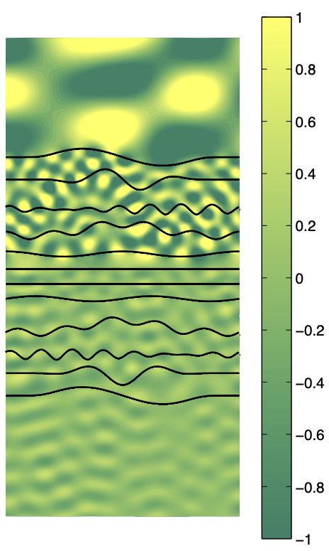
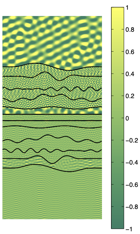
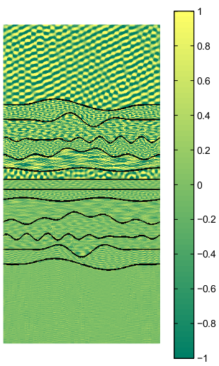
Finally, in Figure 5 we present an illustration of the total field corresponding to the refraction indices given in Table 1.
Remark 6.1.
Though establishing the relation between the parameters— and —and the number of basis elements required to attain a certain desired accuracy is not straightforward, our experiments suggest that should be chosen proportional to the maximum wavenumber .
7 Conclusions
We have proposed a fast spectral method for the efficient representation, through surface potentials based on the quasi-periodic Green’s function, for the solution of the Helmholtz equation with transmission boundary conditions on a periodic domain. Theorem 5.2, we obtained convergence estimates for the discrete approximation of the corresponding boundary data, and found that discrete solution converge at a super-algebraic rate to continuous solutions of the considered boundary integral equation. Though, we focused on the Helmholtz transmission problem, our approximation results and convergence estimates can be easily extended to other boundary integral equations on quasi-periodic Sobolev spaces whenever the formulation is well posed. We avoided Rayleigh-Wood anomalies from our analysis since the series in (5) fails to converge for said frequencies and, for the same reason, our previous results from [5] exclude them as well.
Though similar numerical results are known for the Nyström Method, theoretical results confirming the observed convergence rates are scarce [12], which is an advantage of Galerkin discretizations such as that presented in this article. Moreover, the convergence rate for the proposed discretization is equal to that expected of Nyström methods, so that it is numerically competitive with them while inheriting the theoretical benefits of a Galerkin discretization.
References
- [1] Abramowitz, M., and Stegun, I. A. Handbook of mathematical functions: with formulas, graphs, and mathematical tables, vol. 55. Courier Corporation, 1965.
- [2] Ammari, H. Scattering of waves by thin periodic layers at high frequencies using the on-surface radiation condition method. IMA journal of Applied Mathematics 60, 2 (1998), 199–214.
- [3] Ammari, H., and Bao, G. Coupling of finite element and boundary element methods for the scattering by periodic chiral structures. Journal of Computational Mathematics 26, 3 (March 2008), 261–283.
- [4] Ammari, H., and Nédélec, J.-C. Analysis of the diffraction from chiral gratings. In Mathematical modeling in optical science. SIAM, 2001, pp. 179–206.
- [5] Aylwin, R., Jerez-Hanckes, C., and Pinto, J. On the properties of quasi-periodic boundary integral operators for the helmholtz equation. Integral Equations and Operator Theory 92, 2 (2020), 17.
- [6] Aylwin, R., Silva-Oelker, G., Jerez-Hanckes, C., and Fay, P. Optimization methods for achieving high diffraction efficiency with perfect electric conducting gratings. J. Opt. Soc. Am. A 37, 8 (Aug 2020), 1316–1326.
- [7] Bao, G. Variational approximation of Maxwell’s equations in biperiodic structures. SIAM Journal on Applied Mathematics 57, 2 (1997), 364–381.
- [8] Bao, G. Recent mathematical studies in the modeling of optics and electromagnetics. Journal of Computational Mathematics 22, 2 (2004), 148–155.
- [9] Bao, G., and Dobson, D. C. On the scattering by a biperiodic structure. Proceedings of the American Mathematical Society 128, 9 (April 2000), 2715–2723.
- [10] Bao, G., Dobson, D. C., and Cox, J. A. Mathematical studies in rigorous grating theory. Journal of the Optical Society of America A 12, 5 (1995), 1029–1042.
- [11] Barnett, A., and Greengard, L. A new integral representation for quasi-periodic scattering problems in two dimensions. BIT Numerical mathematics 51, 1 (2011), 67–90.
- [12] Boubendir, Y., Dominguez, V., and Turc, C. High-order nyström discretizations for the solution of integral equation formulations of two-dimensional helmholtz transmission problems. IMA Journal of Numerical Analysis 36 (04 2014).
- [13] Bruno, O. P., and Delourme, B. Rapidly convergent two-dimensional quasi-periodic Green function throughout the spectrum—including Wood anomalies. Journal of Computational Physics 262 (2014), 262–290.
- [14] Bruno, O. P., and Fernandez-Lado, A. G. Rapidly convergent quasi-periodic Green functions for scattering by arrays of cylinders—including Wood anomalies. Proc. R. Soc. A 473, 2199 (2017), 20160802.
- [15] Bruno, O. P., and Haslam, M. C. Efficient high-order evaluation of scattering by periodic surfaces: deep gratings, high frequencies, and glancing incidences. JOSA A 26, 3 (2009), 658–668.
- [16] Bruno, O. P., Shipman, S. P., Turc, C., and Stephanos, V. Three-dimensional quasi-periodic shifted Green function throughout the spectrum, including Wood anomalies. Proc. R. Soc. A 473, 2207 (2017), 20170242.
- [17] Bruno, O. P., Shipman, S. P., Turc, C., and Venakides, S. Superalgebraically convergent smoothly windowed lattice sums for doubly periodic green functions in three-dimensional space. Proc. R. Soc. A 472, 2191 (2016), 20160255.
- [18] Chen, Y.-B., and Zhang, Z. Design of tungsten complex gratings for thermophotovoltaic radiators. Optics communications 269, 2 (2007), 411–417.
- [19] Cho, M. H., and Barnett, A. H. Robust fast direct integral equation solver for quasi-periodic scattering problems with a large number of layers. Optics Express 23, 2 (2015), 1775–1799.
- [20] Colton, D., and Kress, R. Integral Equation Methods in Scattering Theory. Society for Industrial and Applied Mathematics, Philadelphia, PA, 2013.
- [21] Dobson, D. C., and Friedman, A. The time-harmonic Maxwell equations in a doubly periodic structure. Journal of Mathematical Analysis and Applications 166, 2 (1992), 507–528.
- [22] Elschner, J., and Schmidt, G. Diffraction in periodic structures and optimal design of binary gratings. part i: direct problems and gradient formulas. Mathematical Methods in the Applied Sciences 21, 14 (1998), 1297–1342.
- [23] Graham, I. G., and Sloan, I. H. Fully discrete spectral boundary integral methods for Helmholtz problems on smooth closed surfaces in . Numerische Mathematik 92, 2 (2002), 289–323.
- [24] Greengard, L., Ho, K. L., and Lee, J.-Y. A fast direct solver for scattering from periodic structures with multiple material interfaces in two dimensions. Journal of Computational Physics 258 (2014), 738–751.
- [25] Hu, F. Q. A spectral boundary integral equation method for the 2d Helmholtz equation. Journal of Computational Physics 120, 2 (1995), 340 – 347.
- [26] Jerez-Hanckes, C., and Pinto, J. High-order Galerkin method for Helmholtz and Laplace problems on multiple open arcs. Tech. Rep. 2018-49, Seminar for Applied Mathematics, ETH Zürich, Switzerland, 2018.
- [27] Kirsch, A. Diffraction by periodic structures. In Inverse problems in mathematical physics. Springer, 1993, pp. 87–102.
- [28] Kress, R. Linear Integral Equations, third edition ed., vol. 82. Applied Mathematical Sciences, 2014.
- [29] Linton, C. M. The Green’s function for the two-dimensional Helmholtz equation in periodic domains. Journal of Engineering Mathematics 33, 4 (May 1998), 377–401.
- [30] Liu, Y., and Barnett, A. Efficient numerical solution of acoustic scattering from doubly-periodic arrays of axisymmetric objects. Journal of Computational Physics 324 (2016), 226–245.
- [31] Loewen, E. G., and Popov, E. Diffraction gratings and applications. CRC Press, 2018.
- [32] McLean, W. C. H. Strongly Elliptic Systems and Boundary Integral Equations. Cambridge University Press, 2000.
- [33] Nakata, Y., and Koshiba, M. Boundary-element analysis of plane-wave diffraction from groove-type dielectric and metallic gratings. JOSA A 7, 8 (1990), 1494–1502.
- [34] Nédélec, J. C., and Starling, F. Integral equation methods in a quasi-periodic diffraction problem for the time-harmonic Maxwell’s equations. SIAM Journal on Mathematical Analysis 22, 6 (November 1991), 1679–1701.
- [35] Nguyen, D. Spectral methods for direct and inverse scattering from periodic structures.
- [36] Popov, E. Gratings: theory and numeric applications. Popov, Institut Fresnel, 2012.
- [37] Saranen, J., and Vainikko, G. Periodic integral and pseudodifferential equations with numerical approximation. Springer Science & Business Media, 2013.
- [38] Sauter, S. A., and Schwab, C. Boundary Element Methods, vol. 39. Springer Series in Computational Mathematics, 2011.
- [39] Silva, G., Jerez-Hanckes, C., and Fay, P. High-temperature tungsten-hafnia optimized selective thermal emitters for thermophotovoltaic applications. Journal of Quantitative Spectroscopy & Radiative Transfer 231 (2019), 61–68.
- [40] Silva-Oelker, G., Aylwin, R., Jerez-Hanckes, C., and Fay, P. Quantifying the impact of random surface perturbations on reflective gratings. IEEE Transactions on Antennas and Propagation 66, 2 (2018), 838–847.
- [41] Starling, F., and Bonnet-Bendhia, A.-S. Guided waves by electromagnetic gratings and non-uniqueness examples for the diffraction problem. Mathematical Methods in the Applied Sciences 17 (April 1994), 305–338.
- [42] Steinbach, O. Numerical Approximation Methods for Elliptic Boundary Value Problems. Springer Science & Business Media, 2007.
- [43] Taibleson, M. Fourier coefficients of functions of bounded variation. In Proc. Amer. Math. Soc (1967), vol. 18.
- [44] Trefethen, L. N. Spectral Methods in MatLab. Society for Industrial and Applied Mathematics, USA, 2000.
- [45] Zhang, B., and Chandler-Wilde, S. N. A uniqueness result for scattering by infinite rough surfaces. SIAM Journal on Applied Mathematics 58, 6 (1998), 1774–1790.
- [46] Zhang, Y., and Gillman, A. A fast direct solver for two dimensional quasi-periodic multilayered medium scattering problems. arXiv preprint arXiv:1907.06223 (2019).