Excited-state quantum phase transitions in spinor Bose-Einstein condensates

August 11, 2026

Quantum phase transitions (QPTs) are sudden changes in the ground-state properties of a system. The ground-state energy and wave function behave non-analytically and the gap between the ground state and the first excited state closes when, at zero temperature, a control parameter is adiabatically varied across a critical value Sachdev 2011. The idea of QPTs has been extended in recent years to out-of-equilibrium quantum many-body systems Diehl et al. 2010; Heyl 2018. For example, a sudden shift of a parameter (quantum quench), can lead to dynamical QPTs, which are characterized by a non-analyticity of physical quantities as a function of time Heyl 2018. A direct generalization of QPTs beyond the ground state is given by excited-state quantum phase transitions (ESQPTs) Cejnar et al. 2006; Caprio et al. 2008; Cejnar et al. 2020. Their distinguishing signature is a closing gap at nonzero energies: excited states cluster at a critical energy, which leads to a singularity in the density of states (DOS). Typically, the critical energy is a continuous function of a control parameter. Thus, in contrast to ground-state QPTs, ESQPTs can be crossed both by varying a control parameter at constant energy and by varying the energy at fixed parameters.

ESQPTs have been theoretically studied in a large variety of many-body quantum systems Caprio et al. 2008; Stránský et al. 2014; Stránský et al. 2015, including the Lipkin-Meshkov-Glick (LMG) model Leyvraz and Heiss 2005, Dicke and Jaynes-Cummings models Pérez-Fernández et al. 2011; Brandes 2013, interacting boson models Cejnar et al. 2006; Caprio et al. 2008; Macek et al. 2019, molecular bending transitions Pérez-Bernal and Iachello 2008; Larese and Iachello 2011, and the quasi-energy spectrum of driven systems Bastidas et al. 2014. Experimentally, ESQPTs have been confirmed in microwave Dirac billiards Dietz et al. 2013 and in molecular spectroscopy Zobov et al. 2005; Winnewisser et al. 2005. Signatures of ESQPTs have been predicted in the many-body dynamics after a quench Pérez-Fernández et al. 2011; Santos and Pérez-Bernal 2015; Kloc et al. 2018 and in time-averaged expectation values Engelhardt et al. 2015. However, identifying order parameters that distinguish neighboring excited-state quantum phases from each other remains a challenge Cejnar et al. 2006; Caprio et al. 2008.

Spinor Bose-Einstein condensates (BECs) attract since several years a major interest as an exceptional tool for the study of many-body quantum dynamics Kawaguchi and Ueda 2012; Stamper-Kurn and Ueda 2013, including coherent spinor dynamics Chang et al. 2005, classical bifurcations Zibold et al. 2010, and the generation of highly-entangled many-body states Lücke et al. 2011; Gross et al. 2011; Luo et al. 2017; Pezzè et al. 2019. So far systematic investigations of critical behavior in such systems have focused on the ground-state QPTs Kawaguchi and Ueda 2012; Liu et al. 2009; Bookjans et al. 2011; Zhang and Duan 2013; Luo et al. 2017, though observations of diverging oscillation periods can be interpreted as signatures of ESQPTs Zhang et al. 2005; Zhao et al. 2014. Very recently, a study of the quench dynamics of a spinor BEC revealed a dynamical QPT, which has been related to a phase transition in the highest-energy level Tian et al. 2020.

In this Letter, we propose spinor BECs as a platform to explore ESQPTs in a paradigmatic class of models. We identify ESQPTs in a ferromagnetic spin-1 BEC, and show that the different excited-state quantum phases can be distinguished by the topology of classical phase-space trajectories. We use this to introduce an order parameter that is related to the dynamics of coherent states. This order parameter can be accessed by interferometry in existing experimental setups. Our work is, hence, an important step towards the characterization of excited-state quantum phases and towards the systematic exploration of ESQPTs with controllable many-body quantum systems.

Ground-state quantum phases.—We consider a ferromagnetic spin-$1$ BEC of $N$ atoms with three spin states $m=\pm 1,0$. We assume a tight enough external trapping of the BEC such that, to a good approximation, all spin states share a common spatial mode (single-mode approximation). The spin degrees of freedom are then well described by the Hamiltonian density Kawaguchi and Ueda 2012

where $\hat{a}_{m}^{\dagger}$ and $\hat{a}_{m}$ are the bosonic creation and annihilation operators for state $m$, $\hat{N}_{m}\equiv\hat{a}^{\dagger}_{m}\hat{a}_{m}$ with $\sum_{m}\hat{N}_{m}=N$, and $\hat{D}\equiv\hat{N}_{1}-\hat{N}_{-1}$ is the magnetization. The interaction strength $c$ depends on the spatial wave function and on the mass and scattering lengths of the atoms. A ferromagnetic BEC is characterized by $c<0$ Kawaguchi and Ueda 2012. The effective quadratic Zeeman shift $q$ incorporates microwave dressing and thus may be both positive and negative Zhao et al. 2014. The linear Zeeman effect has been eliminated by moving to a rotating frame. The Hamiltonian density (1) conserves $\hat{D}$ and the parity $\hat{I}=(-1)^{\hat{N}_{0}}$. In the eigenspace of $\hat{D}$ with eigenvalue $D=0$, $\hat{h}$ features three ground-state phases Kawaguchi and Ueda 2012; Luo et al. 2017 depending on the ratio $\xi\equiv\frac{q}{2|c|}$: the Twin-Fock (TF) phase for $\xi<-1$, the Polar (P) phase for $\xi>1$, and the Broken-Axisymmetry (BA) phase for $|\xi|<1$.

Excited-state quantum phases.—To reveal the excited-state phases, we study the mean-field limit Raggio and Werner 1989; Duffield and Werner 1992a; Duffield and Werner 1992b; app $N\to\infty$ of Model (1) for the case of zero magnetization. We introduce the coherent states $|\bm{\alpha},N\rangle\equiv\frac{1}{\sqrt{N!}}(\sum_{m}\alpha_{m}\hat{a}_{m}^{\dagger})^{N}|0\rangle$, where $\bm{\alpha}\equiv(\alpha_{1},\alpha_{0},\alpha_{-1})$, $\alpha_{m}\equiv\sqrt{n_{m}}\operatorname{e}^{i\phi_{m}}$, $n_{m}\geq 0$, $\phi_{m}\in[0,2\pi)$, and $\sum_{m}\!n_{m}=1$. The coherent states with $\langle\hat{D}\rangle=0$, i. e., $|\alpha_{1}|^{2}=|\alpha_{-1}|^{2}$, yield the classical Hamiltonian app

where $\phi\equiv\phi_{0}-(\phi_{1}+\phi_{-1})/2$. Note that parity conservation results in $h_{\mathrm{mf}}(\phi+\pi)=h_{\mathrm{mf}}(\phi)$. The mean-field dynamics is governed by the equations of motion Kawaguchi and Ueda 2012; Zhang et al. 2005; app

with $\tau\equiv|c|t/\hbar$. The mean-field limit of the DOS $\nu_{0}(\eta)$ in the $D=0$ subspace can be computed according to app

where $\mathcal{D}\bm{\alpha}\equiv\frac{1}{(2\pi)^{3}}\prod_{m}\!\operatorname{d}\!n_{m}\!\operatorname{d}\!\phi_{m}\,\delta\!\left(\sum_{m}\!n_{m}-1\right)$ and $\eta$ denotes the energy divided by $N|c|$. Below we employ Eqs. (3) and (4) to study the signatures of ESQPTs.

Extending the ground-state phase diagram to the entire energy spectrum, we identify three excited-state phases in the $\xi$-$\eta$-plane: the TF^′ phase for $\eta>-|\xi|$ and $\xi<0$, the P^′ phase for $\eta>-|\xi|$ and $\xi>0$, and the BA^′ phase for $\eta<-|\xi|$. The phases are indicated in Fig. 1a, where we have subtracted $\eta_{0}(\xi)=-\frac{1}{2}(\xi^{2}+1)$, which corresponds to the ground-state energy in the mean-field limit, from $\eta$. The excited-state phases are separated by ESQPTs at $\eta_{*}=-|\xi|$ with $0<|\xi|<1$. In the limit $|\xi|\to 0$, $\eta_{*}$ hits the maximum of $h_{\mathrm{mf}}/|c|$. As $|\xi|$ approaches $1$, the ESQPTs evolve into the known ground-state QPTs.

Signatures of ESQPTs.—As expected for ESQPTs Cejnar et al. 2006; Caprio et al. 2008, the DOS (4) diverges at $\eta_{*}(\xi)$. Fig. 1a displays the mean-field DOS as a function of $\xi$ and $\eta-\eta_{0}$. Furthermore, it shows that in a finite-size system the ESQPTs reveal themselves by a sequence of avoided crossings in the energy spectrum Cejnar et al. 2006. The divergence of the DOS is due to stationary points of $h_{\mathrm{mf}}$. At a stationary point, $\frac{\partial}{\partial\phi}h_{\mathrm{mf}}=\frac{\partial}{\partial n_{0}}h_{\mathrm{mf}}=0$ causes the integrand in Eq. (4) to become singular. There are three stationary points at each $0<|\xi|<1$: a saddle point at $\eta_{*}$ and two minima at $\eta_{0}$. The saddle point is located at $n_{0}=0$ for $\xi<0$ or at $n_{0}=1$ for $\xi>0$, and the minima are at $n_{0}=(\xi+1)/2$ and $\cos^{2}(\phi)=1$, see Fig. 1b. Note that these stationary points do not depend on the restriction to coherent states with $\langle\hat{D}\rangle=0$. However, the unrestricted DOS app remains finite at $\eta_{*}$.

The phase-space trajectories app of $h_{\mathrm{mf}}$ provide further signatures of the ESQPTs. The classical phase space is a sphere with $z$-axis $n_{0}$ and azimuthal angle $\phi$. Figure 1b shows exemplary trajectories for $\xi=0.5$. The trajectories reflect the symmetry $h_{\mathrm{mf}}(\phi+\pi)=h_{\mathrm{mf}}(\phi)$. Since $h_{\mathrm{mf}}(\xi,n_{0},\phi)=h_{\mathrm{mf}}(-\xi,1-n_{0},\phi)$, for $\xi<0$ the phase space would appear upside down. As in the LMG model Ribeiro et al. 2008, the sets of trajectories at fixed $\xi$ and $\eta$ (the energy hypersurfaces) change topology at $\eta_{*}(\xi)$—at the critical energy hypersurfaces called separatrices. For $\eta>\eta_{*}$, i. e., in the TF^′ and P^′ phases, there is only one trajectory per $\xi$ and $\eta$. By contrast, for $\eta<\eta_{*}$, i. e., in the BA^′ phase, the evolution can follow one of two disconnected trajectories. Each of these trajectories breaks the classical symmetry $h_{\mathrm{mf}}(\phi+\pi)=h_{\mathrm{mf}}(\phi)$. Note, however, that the corresponding quantum symmetry $I$ cannot be broken in the $D=0$ subspace, where all states belong to a single eigenspace of $I$.

Order parameter.—The solutions $n_{0}(t)$ and $\phi(t)$ of the classical equations of motion, Eq. (3), are periodic Kawaguchi and Ueda 2012; Zhang et al. 2005; app. In the TF^′ and P^′ phases, the phase-space trajectories encircle the $n_{0}$-axis (green curves in Fig. 1b)—clockwise in the TF^′ phase and counterclockwise in the P^′ phase. By contrast, the trajectories in the BA^′ phase do not enclose the $n_{0}$-axis (yellow curves). We define our order parameter $w$ as the winding number of the classical trajectories with respect to the $n_{0}$-axis, such that $w=-1$ in the TF^′, $w=1$ in the P^′, and $w=0$ in the BA^′ phase. We observe that $w$ can be expressed in a particularly simple form. Let us denote the period of $n_{0}(t)$ at fixed $\xi$ and $\eta$ by $T$. In the BA^′ phase, the periods of $\phi(t)$ and $n_{0}(t)$ coincide and, thus, $\phi(t+T)=\phi(t)$. In the TF^′ and P^′ phases, however, $\phi(t+T)=\phi(t)\pm\pi$. Hence,

In contrast to most observables that have been studied in the context of ESQPTs Heiss et al. 2005; Ribeiro et al. 2008; Brandes 2013; Caprio et al. 2008; Pérez-Fernández et al. 2011; Bastidas et al. 2014; Santos and Pérez-Bernal 2015; Kloc et al. 2018, $w$ is not merely singular at the phase transitions. It qualitatively distinguishes the entire excited-state phases by the dynamics of coherent states.

In the following, we present an interferometric scheme that extracts

and therefore distinguishes neighboring excited-state phases from each other: in the BA^′ phase $p=1$, while in the TF^′ and P^′ phases $p=-1$. To measure $p$, first, an initial point $(n_{0}(0),\phi(0))$ on a trajectory at the $\xi$ and $\eta$ of interest is selected. Then the corresponding coherent state with $\phi_{1}=\phi_{-1}$, $|\psi(0)\rangle$, is prepared at $q=2|c|\xi$. The state freely evolves for the time $T$. Next, the spin states $m=0$ and $m=\pm 1$ are coupled by the internal-state beamsplitter $\exp(-i\frac{\pi}{2}\hat{S}_{\theta_{0}})$ with $\hat{S}_{\theta}\equiv\frac{1}{2}(\operatorname{e}^{-i\theta}\hat{a}_{0}^{\dagger}\hat{g}+\operatorname{e}^{i\theta}\hat{g}^{\dagger}\hat{a}_{0})$, $\hat{g}\equiv(\hat{a}_{1}+\hat{a}_{-1})/\sqrt{2}$, and $\theta_{0}\equiv\pi/2-\phi(0)$. Finally, the expectation value of $\hat{N}_{0}/N$ is measured. In the mean-field limit, this yields app

where we have introduced the visibility $V=2\sqrt{1-n_{0}(0)}\sqrt{n_{0}(0)}$. As long as $n_{0}(0)\neq 0,1$, this unambiguously determines $p$.

Experimental realization.—We detail the measurement of $p$ for ⁸⁷Rb atoms in their hyperfine ground state Lücke et al. 2011; Luo et al. 2017. However, most of our discussion applies to any ferromagnetic spin-$1$ BEC. We assume that, initially, the condensate is in the state $\hat{a}_{0}^{\dagger N}|0\rangle/\sqrt{N!}$. Then a coherent state characterized by $n_{0}(0)$, $\phi(0)$, and $\phi_{1}=\phi_{-1}$ can be obtained by applying $\exp(-i\chi\hat{S}_{{\theta_{0}}})$ with $\cos^{2}(\chi/2)=n_{0}(0)$. Thus, both the state preparation and the beamsplitter are generated by $\hat{S}_{{\theta_{0}}}$ and can be implemented by a sequence of a phase shift $\exp(i({\theta_{0}}-\theta_{\mathrm{rf}})\hat{N}_{0})$, a radio-frequency pulse $\exp(-i\zeta\hat{S}_{\theta_{\mathrm{rf}}})$ ¹¹ 1 The phase $\theta_{\mathrm{rf}}$ is fundamentally fixed by the interaction of the atoms with the radio-frequency pulse. While we do not state its value, it may be both derived and measured. with $\zeta=\chi$ or $\zeta=\pi/2$, respectively, and another phase shift $\exp(-i({\theta_{0}}-\theta_{\mathrm{rf}})\hat{N}_{0})$. Since we aim at the expectation value in Eq. (7), the first step of the state preparation and the last one of the beamsplitter can be omitted. $N_{0}$ can be measured, e. g., by a magnetic-field gradient that spatially separates the different spin states and subsequent absorptive imaging.

Reliably distinguishing $p=\pm 1$ requires a large visibility $V$, which can be maximized by choosing $n_{0}(0)$ as close to $1/2$ as possible. The optimal $n_{0}(0)$, $n_{\mathrm{opt}}$, is app:

A corresponding $\phi(0)$, $\phi_{\mathrm{opt}}$, is obtained from

Figure 2a shows that the optimized visibility is large throughout the vast majority of the phase diagram.

The coherence time in typical BEC experiments is limited to few seconds. This constrains the accessible periods $T$. It is known Kawaguchi and Ueda 2012; Zhang et al. 2005; app that

where $K(k^{2})=\int_{0}^{\pi/2}\operatorname{d}\!\gamma\sqrt{1-k^{2}\sin^{2}\!\gamma}^{-1}$ is the complete elliptic integral of the first kind, $x=|\xi|\sqrt{1+\xi^{2}+2\eta}$, and $y=(x-\xi^{2}-\eta)/2$. $T$ diverges at the ESQPTs. Figure 2b displays $T$ for the typical interaction strength $|c|/\hbar=2\pi\times$4\text{\,}\mathrm{H}\mathrm{z}$$. Fortunately, $T$ exceeds a moderate value of, e. g., $0.3\text{\,}\mathrm{s}$ only in the immediate vicinity of the ESQPTs.

So far we have considered only the mean-field limit, $N\to\infty$. To study the impact of a finite system size, we simulate a measurement of $p$ for $N=100$ bosons by exact diagonalization of the Hamiltonian density (1), see Fig. 3. The jump discontinuities signaling the ESQPTs in the mean-field limit are, as expected, smoothed at finite $N$. However, the BA^′ phase can still be clearly distinguished from the TF^′ and P^′ phases. In typical experiments, $N$ is of the order of $10^{4}$ and, thus, a much better convergence to the mean-field limit can be expected.

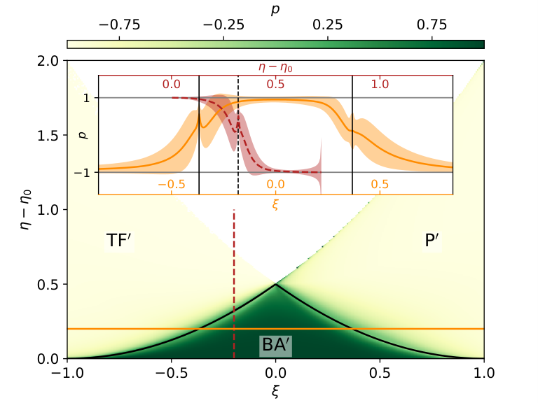
Conclusions.—Ferromagnetic spin-$1$ BECs exhibit ESQPTs, which, in the mean-field limit, show up as a diverging DOS and a change in the topology of phase-space trajectories. We characterize the mean-field dynamics by a winding number $w$ that distinguishes the excited-state quantum phases from each other and, thus, is an order parameter. Adjacent phases differ in $|w|$ and can be told apart by interferometrically monitoring the coherent many-body dynamics in present-day experiments. Note that the local order parameter $\hat{N}_{0}/N$ that characterizes the ground-state QPTs Zhang and Duan 2013; Luo et al. 2017 cannot be directly generalized to excited states. The topological order parameter $w$, instead, is defined for all energies apart from the very ground state, where the trajectories reduce to single points. Our results show that ESQPTs can be studied in well-controlled atomic quantum many-body systems, and that these studies are not limited to properties of the transition itself. We propose a feasible experiment for characterizing excited-state quantum phases. This represents an important step towards employing ESQPTs in quantum state engineering.

Finally, we remark that our findings apply to any of the numerous quantum systems with the same mean-field limit, including bosonic two-level pairing models at zero generalized angular momentum Caprio et al. 2008. Our theoretical treatment of ESQPTs complements previous studies for opposite interaction sign Caprio et al. 2008. Bosonic two-level pairing models comprise, e. g., the LMG model, the vibron model for molecules, and the interacting boson model for nuclei.

We thank Dmytro Bondarenko, Pavel Cejnar, Ignacio Cirac, and Reinhard Werner for valuable discussions. We acknowledge support by the Deutsche Forschungsgemeinschaft (DFG, German Research Foundation) under the SFB 1227 “DQ-mat”, project A02, and under Germany’s Excellence Strategy – EXC-2123 QuantumFrontiers – 390837967, and by the LabEx ENS-ICFP: ANR-10-LABX-0010/ANR-10-IDEX-0001-02 PSL*.

References

- Sachdev (2011) S. Sachdev, Quantum Phase Transitions, 2nd ed. (Cambridge University Press, 2011).
- Diehl et al. (2010) Sebastian Diehl, Andrea Tomadin, Andrea Micheli, Rosario Fazio, and Peter Zoller, “Dynamical phase transitions and instabilities in open atomic many-body systems,” Phys. Rev. Lett. 105, 015702 (2010).
- Heyl (2018) M. Heyl, “Dynamical quantum phase transitions: a review,” Rep. Prog. Phys. 81, 054001 (2018).
- Cejnar et al. (2006) P. Cejnar, M. Macek, S. Heinze, J. Jolie, and J. Dobeš, “Monodromy and excited-state quantum phase transitions in integrable systems: collective vibrations of nuclei,” J. of Phys. A 39, L515–L521 (2006).
- Caprio et al. (2008) M. A. Caprio, P. Cejnar, and F. Iachello, “Excited state quantum phase transitions in many-body systems,” Annals of Physics 323, 1106 – 1135 (2008).
- Cejnar et al. (2020) P. Cejnar, P. Stránský, M. Macek, and M. Kloc, “Excited-state quantum phase transitions,” arXiv:2011.01662 (2020).
- Stránský et al. (2014) P. Stránský, M. Macek, and P. Cejnar, “Excited-state quantum phase transitions in systems with two degrees of freedom: Level density, level dynamics, thermal properties,” Ann. Phys. 345, 73–97 (2014).
- Stránský et al. (2015) P. Stránský, M. Macek, A. Leviatan, and P. Cejnar, “Excited-state quantum phase transitions in systems with two degrees of freedom: II. finite-size effects,” Annals of Physics 356, 57 – 82 (2015).
- Leyvraz and Heiss (2005) F. Leyvraz and W. D. Heiss, “Large- scaling behavior of the lipkin-meshkov-glick model,” Phys. Rev. Lett. 95, 050402 (2005).
- Pérez-Fernández et al. (2011) P. Pérez-Fernández, P. Cejnar, J. M. Arias, J. Dukelsky, J. E. García-Ramos, and A. Relaño, “Quantum quench influenced by an excited-state phase transition,” Phys. Rev. A 83, 033802 (2011).
- Brandes (2013) T. Brandes, “Excited-state quantum phase transitions in dicke superradiance models,” Phys. Rev. E 88, 032133 (2013).
- Macek et al. (2019) M. Macek, P. Stránský, A. Leviatan, and P. Cejnar, “Excited-state quantum phase transitions in systems with two degrees of freedom. III. interacting boson systems,” Phys. Rev. C 99, 064323 (2019).
- Pérez-Bernal and Iachello (2008) F. Pérez-Bernal and F. Iachello, “Algebraic approach to two-dimensional systems: Shape phase transitions, monodromy, and thermodynamic quantities,” Phys. Rev. A 77, 032115 (2008).
- Larese and Iachello (2011) D. Larese and F. Iachello, “A study of quantum phase transitions and quantum monodromy in the bending motion of non-rigid molecules,” J. of Mol. Struct. 1006, 611–628 (2011).
- Bastidas et al. (2014) V. M. Bastidas, P. Pérez-Fernández, M. Vogl, and T. Brandes, “Quantum criticality and dynamical instability in the kicked-top model,” Phys. Rev. Lett. 112, 140408 (2014).
- Dietz et al. (2013) B. Dietz, F. Iachello, M. Miski-Oglu, N. Pietralla, A. Richter, L. von Smekal, and J. Wambach, “Lifshitz and excited-state quantum phase transitions in microwave dirac billiards,” Phys. Rev. B 88, 104101 (2013).
- Zobov et al. (2005) Nikolai F. Zobov, Sergei V. Shirin, Oleg L. Polyansky, Jonathan Tennyson, Pierre-François Coheur, Peter F. Bernath, Michel Carleer, and Reginald Colin, “Monodromy in the water molecule,” Chemical Physics Letters 414, 193 (2005).
- Winnewisser et al. (2005) Brenda P. Winnewisser, Manfred Winnewisser, Ivan R. Medvedev, Markus Behnke, Frank C. De Lucia, Stephen C. Ross, and Jacek Koput, “Experimental confirmation of quantum monodromy: The millimeter wave spectrum of cyanogen isothiocyanate ncncs,” Phys. Rev. Lett. 95, 243002 (2005).
- Santos and Pérez-Bernal (2015) L. F. Santos and F. Pérez-Bernal, “Structure of eigenstates and quench dynamics at an excited-state quantum phase transition,” Phys. Rev. A 92, 050101 (2015).
- Kloc et al. (2018) M. Kloc, P. Stránský, and P. Cejnar, “Quantum quench dynamics in dicke superradiance models,” Phys. Rev. A 98, 013836 (2018).
- Engelhardt et al. (2015) G. Engelhardt, V. M. Bastidas, W. Kopylov, and T. Brandes, “Excited-state quantum phase transitions and periodic dynamics,” Phys. Rev. A 91, 013631 (2015).
- Kawaguchi and Ueda (2012) Y. Kawaguchi and M. Ueda, “Spinor Bose–Einstein condensates,” Physics Reports 520, 253 – 381 (2012).
- Stamper-Kurn and Ueda (2013) Dan M. Stamper-Kurn and Masahito Ueda, “Spinor bose gases: Symmetries, magnetism, and quantum dynamics,” Rev. Mod. Phys. 85, 1191–1244 (2013).
- Chang et al. (2005) M.-S. Chang, Q. Qin, W. Zhang, L. You, and M. S. Chapman, “Coherent spinor dynamics in a spin-1 bose condensate,” Nat. Phys. 1, 111–116 (2005).
- Zibold et al. (2010) T. Zibold, E. Nicklas, C. Gross, and M. K. Oberthaler, “Classical bifurcation at the transition from rabi to josephson dynamics,” Phys. Rev. Lett. 105, 204101 (2010).
- Lücke et al. (2011) B. Lücke, M. Scherer, J. Kruse, L. Pezzé, F. Deuretzbacher, P. Hyllus, O. Topic, J. Peise, W. Ertmer, J. Arlt, L. Santos, A. Smerzi, and C. Klempt, “Twin matter waves for interferometry beyond the classical limit,” Science 334, 773–776 (2011).
- Gross et al. (2011) C. Gross, H. Strobel, E. Nicklas, T. Zibold, N. Bar-Gill, G. Kurizki, and M. K. Oberthaler, “Atomic homodyne detection of continuous-variable entangled twin-atom states,” Nature 480, 219–223 (2011).
- Luo et al. (2017) X.-Y. Luo, Y.-Q. Zou, L.-N. Wu, Q. Liu, M.-F. Han, M. K. Tey, and L. You, “Deterministic entanglement generation from driving through quantum phase transitions,” Science 355, 620–623 (2017).
- Pezzè et al. (2019) L. Pezzè, M. Gessner, P. Feldmann, C. Klempt, L. Santos, and A. Smerzi, “Heralded generation of macroscopic superposition states in a spinor Bose-Einstein condensate,” Phys. Rev. Lett. 123, 260403 (2019).
- Liu et al. (2009) Y. Liu, S. Jung, S. E. Maxwell, L. D. Turner, E. Tiesinga, and P. D. Lett, “Quantum phase transitions and continuous observation of spinor dynamics in an antiferromagnetic condensate,” Phys. Rev. Lett. 102, 125301 (2009).
- Bookjans et al. (2011) E. M. Bookjans, A. Vinit, and C. Raman, “Quantum phase transition in an antiferromagnetic spinor bose-einstein condensate,” Phys. Rev. Lett. 107, 195306 (2011).
- Zhang and Duan (2013) Z. Zhang and L.-M. Duan, “Generation of massive entanglement through an adiabatic quantum phase transition in a spinor condensate,” Phys. Rev. Lett. 111, 180401 (2013).
- Zhang et al. (2005) W. Zhang, D. L. Zhou, M.-S. Chang, M. S. Chapman, and L. You, “Coherent spin mixing dynamics in a spin-1 atomic condensate,” Phys. Rev. A 72, 013602 (2005).
- Zhao et al. (2014) L. Zhao, J. Jiang, T. Tang, M. Webb, and Y. Liu, “Dynamics in spinor condensates tuned by a microwave dressing field,” Phys. Rev. A 89, 023608 (2014).
- Tian et al. (2020) T. Tian, H.-X. Yang, L.-Y. Qiu, H.-Y. Liang, Y.-B. Yang, Y. Xu, and L.-M. Duan, “Observation of dynamical quantum phase transitions with correspondence in an excited state phase diagram,” Phys. Rev. Lett. 124, 043001 (2020).
- Raggio and Werner (1989) G. A. Raggio and R. F. Werner, “Quantum statistical mechanics of general mean field systems,” Helv. Phys. Acta 62, 980–1003 (1989).
- Duffield and Werner (1992a) N. G. Duffield and R. F. Werner, “Mean-field dynamical semigroups on -algebras,” Rev. Math. Phys. 4, 383–424 (1992a).
- Duffield and Werner (1992b) N. G. Duffield and R. F. Werner, “Classical Hamiltonian dynamics for quantum Hamiltonian mean-field limits,” in Stochastics and quantum mechanics, Proceedings of a conference held in Swansea, UK, 1986, edited by A. Truman and I. M. Davies (World Sci. Publishing, 1992) pp. 115–129.
- (39) See Appendix for details on the mean-field limit of bosonic systems in general and of ferromagnetic spin-1 BECs in particular.
- Ribeiro et al. (2008) P. Ribeiro, J. Vidal, and R. Mosseri, “Exact spectrum of the lipkin-meshkov-glick model in the thermodynamic limit and finite-size corrections,” Phys. Rev. E 78, 021106 (2008).
- Heiss et al. (2005) W. D. Heiss, F. G. Scholtz, and H. B. Geyer, “The large-N behaviour of the Lipkin model and exceptional points,” J. of Phys. A 38, 1843–1851 (2005).
- Loya (2017) P. Loya, Amazing and aesthetic aspects of analysis (Springer, New York, NY, 2017).
- Königsberger (2004) K. Königsberger, Analysis, 5th ed., Vol. 2 (Springer, Berlin, Heidelberg, 2004).
- Forster (2013) O. Forster, Analysis, 11th ed., Vol. 1 (Springer Spektrum, Wiesbaden, 2013).
- Feldmann et al. (2018) P. Feldmann, M. Gessner, M. Gabbrielli, C. Klempt, L. Santos, L. Pezzè, and A. Smerzi, “Interferometric sensitivity and entanglement by scanning through quantum phase transitions in spinor bose-einstein condensates,” Phys. Rev. A 97, 032339 (2018).