myctr
CAPTURE STEPS:
ROBUST WALKING FOR HUMANOID ROBOTS
Abstract
Stable bipedal walking is a key prerequisite for humanoid robots to reach their potential of being versatile helpers in our everyday environments. Bipedal walking is, however, a complex motion that requires the coordination of many degrees of freedom while it is also inherently unstable and sensitive to disturbances. The balance of a walking biped has to be constantly maintained. The most effective way of controlling balance are well timed and placed recovery steps—capture steps—that absorb the expense momentum gained from a push or a stumble. We present a bipedal gait generation framework that utilizes step timing and foot placement techniques in order to recover the balance of a biped even after strong disturbances. Our framework modifies the next footstep location instantly when responding to a disturbance and generates controllable omnidirectional walking using only very little sensing and computational power. We exploit the open-loop stability of a central pattern generated gait to fit a linear inverted pendulum model to the observed center of mass trajectory. Then, we use the fitted model to predict suitable footstep locations and timings in order to maintain balance while following a target walking velocity. Our experiments show qualitative and statistical evidence of one of the strongest push-recovery capabilities among humanoid robots to date.
keywords
Bipedal walking; Push recovery; Humanoid robots; Linear inverted pendulum model.- UML
- Unified Modeling Language
- CoM
- Center of Mass
- CoP
- Center of Pressure
- CPG
- Central Pattern Generator
- LIPM
- Linear Inverted Pendulum Model
- TDA
- Trunk Deviation Angle
- IMU
- Inertial Measurement Unit
- ZMP
- Zero Moment Point
1 Introduction
Bipedal walking is an energy efficient and versatile means of locomotion suitable for covering large distances in a wide variety of terrains. Its principle dynamics can be likened to an inverted pendulum that is constantly falling and requires active control in order to remain balanced—for example by stepping into the right place at the right time. Undoubtedly, it would be of great benefit if we were able to replicate a walking controller with human-like capabilities. Unfortunately, as easy as walking comes to us humans, the design of walking controllers for bipedal robots has proven to be rather challenging. The widespread state of the art covers basic walking on flat surfaces in the absence of disturbances. Push recovery, walking on rough terrain, and agile footstep control are active research topics. The dominant strategy to make a robot walk is to abstract from the complex body and to represent its centroidal momentum with the inverted pendulum model. In most cases, the mathematically tractable Linear Inverted Pendulum Model is used to deduce controllers that steer and balance the pendulum in a way that the ZMP—the assumed pivot point of the inverted pendulum—stays within the boundaries of preset footsteps that have been planned ahead. The trajectory of the point mass model is then transformed into a whole-body walking motion by tracking the pendulum motion with the pelvis, connecting the pendulum base locations with smooth swing foot trajectories in Cartesian space, and computing the resulting motor commands using inverse kinematics. This approach works, but has not yet achieved the versatility and robustness of the human gait.
The bipedal walk generation technique presented here differs from the state of the art in a number of aspects. Instead of designing a low-dimensional model and forcing a robot to follow its motion, we first craft a central pattern-generated (CPG) whole-body motion that can produce an open-loop stable gait. A low-dimensional inverted pendulum model is then fitted to match the observed center of mass trajectory of the open-loop motion. The fitted model can then be used to predict the state of balance at the end of the step, and to compute the location and the timing of a footstep that is expected to restore balance towards a stable limit cycle. Our approach augments the CPG gait with balance control by modifying timing and landing coordinates of footsteps in a non-intrusive way, leaving the execution of the stepping motions up to the underlying pattern generator. The result is a robust and controllable omnidirectional walk that does not derogate the natural dynamics by forcing the center of mass onto a plane—a consequence when a low-dimensional model is imposed on the robot as many other approaches do.
Our algorithm requires very little computational power and only basic sensory equipment. Inertial sensors in the torso are used to estimate its attitude, and joint position sensors are used to reconstruct the pose of the robot. No force or torque sensors are required. A precise robot model is not required either, as masses, torques, and forces are not involved in our computations. A rough kinematic model describing approximate link lengths suffices. We are also able to relax precision requirements on the actuation level. We operate our robot in a compliant setting with low-gain position-controlled actuators. Despite its low requirements, it achieves one of the strongest push recovery capabilities among humanoid robots to date.
2 Related Work
ZMP (ZMP) preview control [Kajita et al. 2003] is the most popular approach to bipedal walking. A number of pre-planned footsteps are used to define a future ZMP reference trajectory. A continuous CoM (CoM) trajectory that minimizes the ZMP tracking error, the jerk of the CoM, and the deviation from terminal conditions at the end of the preview horizon, is then generated by solving a quadratic program [Wieber 2006]. The optimization is computationally expensive, but can be performed in real time. In theory, once a smooth and stable model is computed, a robot closely following the motion of the model should be stable, too. By using the ZMP preview control scheme, high quality robots [Kajita et al. 2010, Ill-Woo Park et al. 2005] can walk on flat ground as long as disturbances are small. More advanced gait controllers from the ZMP preview family [Diedam et al. 2008, Morisawa et al. 2010, Stephens and Atkeson 2010] also consider foot placement in addition to ZMP control by including the footstep locations in the optimization process.
A sampling-based ZMP preview controller that includes adaptive foot-placement has been proposed by Urata et al. 2011. Instead of optimizing the CoM trajectory for a single ZMP reference, a fast sampling method is used to generate a whole set of lower quality ZMP/CoM trajectory pairs for three steps into the future. Triggered by a disturbance, the algorithm selects and executes the best available motion according to given optimization criteria. Resampling during execution of the motion plan is not possible. This method was demonstrated to produce push recovery capabilities on a real robot. Highly specialized hardware was used to meet the speed and precision requirements.
Another interesting planning approach was presented by Kamioka et al. 2019 where walking, running, and hopping are planned in parallel as alternative modes of locomotion. The best plan is selected according to stability and energy consumption criteria. Footstep locations and timing are computed by a gradient decent algorithm during walking.
The capture point [Pratt et al. 2006] is an appealing indicator of balance. It describes the location on the ground where a biped would need to step in order to come to a complete stop. Englsberger et al. 2011 proposed the use of a capture point trajectory as a reference input for gait generation, instead of the ZMP. The capture point approach is much simpler and faster to compute than ZMP preview control. A capture point based preview controller was demonstrated on Toro [Ott et al. 2010] and on the Atlas robot to produce a walk of the same quality as the classic ZMP preview controller.
A drawback of all of the aforementioned approaches is that the motion of a low-dimensional model is computed first, and then the robot is forced to follow its trajectory as closely as possible. This imposes precise position tracking requirements on the hardware in order to preserve the stability predicted by the model. Furthermore, a low-dimensional model strongly simplifies the walking motion by design. Following the model closely results in an unnatural, plane-restricted motion of the pelvis—typically with extensive use of bent knees.
The inverse approach of starting with the motion before balance originates from passive dynamic walking pioneered by McGeer 1990. His experiments proved that the passive dynamics of legs with freewheeling joints is sufficiently stable to walk down a shallow slope. With a minimal amount of actuation to restore lost energy, passive walking on level ground is also possible [Wisse and van Frankenhuyzen 2006, Anderson et al. 2005, Collins et al. 2001]. The graceful motions of these bipedal constructions strongly resemble the human walk and suggest that the core principle of biological gaits may also be passive dynamics with minimal control effort.
CPG walking adds actuation, but no control of balance. However, a small basin of attraction around the upright pose allows for controllable, open-loop stable walking. Interestingly, in the competitive environment of RoboCup, where humanoid robots play soccer, CPG walking is the dominant approach. Perhaps the most advanced RoboCup gait was presented for the Nao standard platform by Graf and Röfer 2012. Based on the solution of a system of linear pendulum equations, the timing and trajectory of the pendulum motion is adjusted online in order to land the swing foot as closely as possible to a desired step size.
The DARwIn-OP platform [Ha et al. 2013] comes with a fast and reliable walk that has been described by Yi et al. 2011. The core gait has a strong similarity with ZMP preview control. Future footstep locations are placed in a queue as reference. However, instead of the expensive CoM trajectory optimization that includes jerk minimization, the CoM trajectory is generated open-loop and in closed form using simple LIPM equations that do not limit the jerk.
By modeling virtual forces that keep the robot upright and pull it in the desired direction of locomotion, Pratt et al. 2001 created the Virtual Model Control approach. The virtual forces are mapped to torques of the actuators such that the same trunk motion is produced as the forces would. With this method, the two-dimensional robot Spring Flamingo showed a fluid and natural looking walk that was robust enough to reject small disturbances and to walk up and down on slopes.
The work presented here has its origins in [Missura and Behnke 2011], where first lateral stability was investigated with the conclusion that controling the step timing is effective at recovering the lateral oscillation after a push from the side. Then, the concept was extended to the sagittal direction in simulation [Missura and Behnke 2013b] and implemented on a real robot [Missura and Behnke 2015b]. Onboard learning of the sagittal step size has also been investigated [Missura and Behnke 2015a] to a degree where a robot was able to learn to absorb a strong push after only a few failed steps.
3 Capture Step Framework
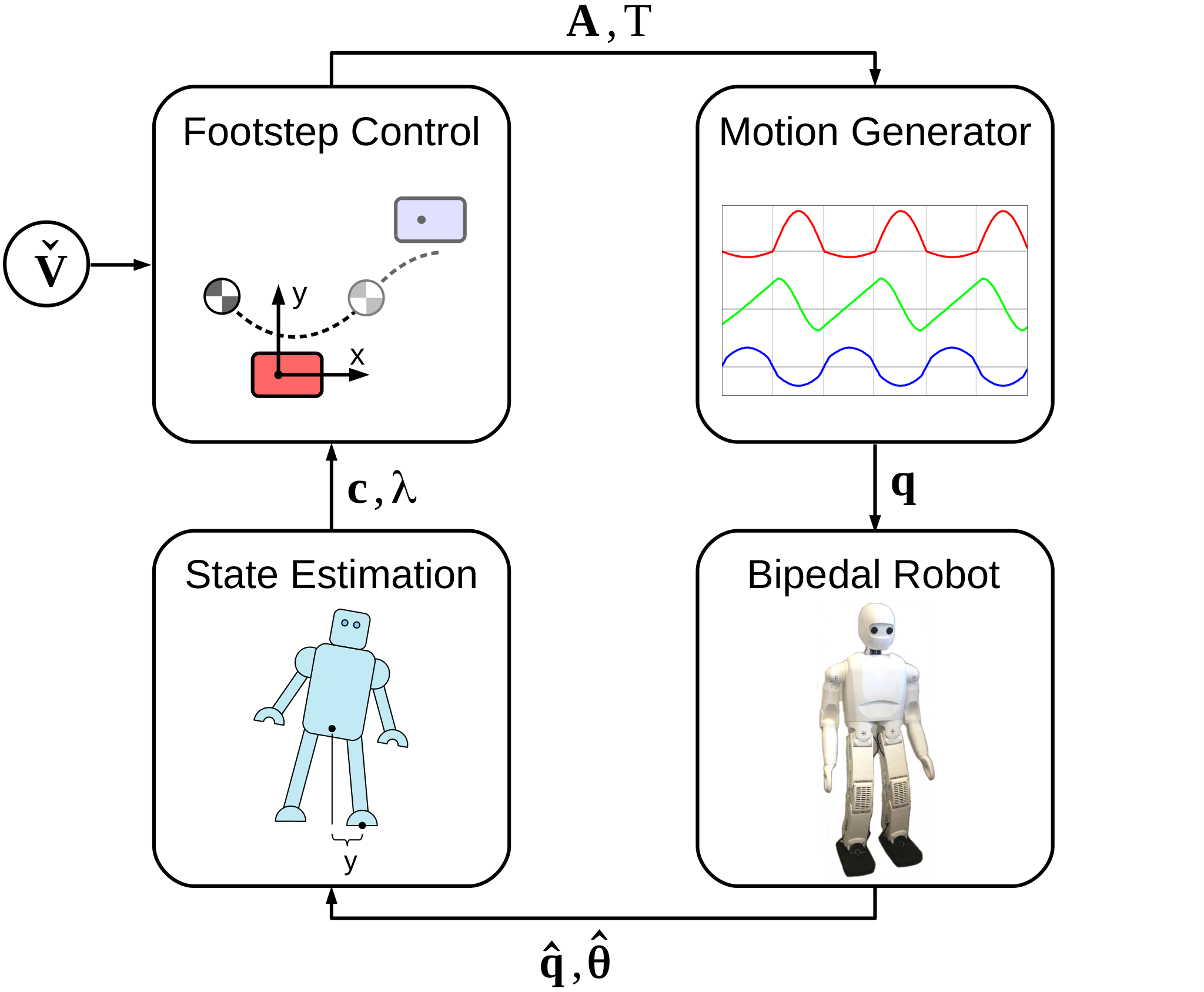
The bipedal gait generation method presented here is called Capture Step Framework. Figure 1 illustrates the components of the framework organized in the circular layout of a control loop. The robot itself is part of the loop. It receives motor targets from the control software and provides sensor data about its internal state. The three main software components are: State Estimation, Footstep Control, and Motion Generation.
The input into the control loop is a target velocity parameter that controls the sagittal, the lateral, and the rotational velocity of the gait. The target velocity determines the size of the steps the robot should produce. The framework attempts to realize the commanded velocity as good as it can, but it may deviate from it in order to maintain balance. Alternatively, it is possible to use a reference step size as input instead of the velocity in order to command the robot to follow a footstep plan [Missura 2016].
The Motion Generator is a CPG that generates whole-body stepping motions composed of superimposed leg-lifting and leg-swinging motion primitives. The motion primitives are parameterized in a way that the footstep location at the end of the step can be controlled by the swing amplitude parameter in the sagittal, lateral, and rotational directions. The timing of the steps is controlled by the step time parameter . In the end, the whole-body motion trajectory is conveniently expressed as a signal of joint angles that are passed on to the robot. The robot tracks the joint angles using PD-controlled servo motors.
Using the joint angles and the torso inclination as measured by the sensors of the robot, the State Estimation module reconstructs the tilted whole-body pose. From the reconstructed pose, the motion of a fixed point on the body frame is tracked and used as a low-dimensional representation of balance. The coordinates and velocities of this fixed point—hereafter referred to as the CoM (CoM) state —are determined in the sagittal (x, forward) and the lateral (y, sideward) directions with respect to the coordinate frame of the support foot with the sign . We assign -1 to the left foot and 1 to the right foot.
The CoM state vector , the sign of the support foot, and the desired velocity , are the inputs into the Footstep Control module, where a LIPM (LIPM) is used to compute the swing amplitude and the time of the next footstep in order to keep the center of mass balanced while obeying the desired velocity as closely as possible. The swing amplitude and the step time become the inputs of the Motion Generator module.
One iteration of the control software loop requires 0.12 ms to compute on a single 1.3 GHz core and thus can be operated with a high frequency. We are using an update frequency of 100 Hz.
In the following, we introduce the modules of the Capture Step Framework shown in Figure 1 in detail.
4 Motion Generator
The nonzero size of the support polygon of a humanoid robot allows for some passive stability that can be exploited to implement stable walking with an open-loop CPG. The NimbRo CPG gait was originally proposed by Behnke 2006 and extended by Missura and Behnke 2013a and Missura 2016. Using oscillating motion patterns for the legs and the arms, the CPG generates an omnidirectional gait that allows a humanoid robot to step in the sagittal, lateral, and rotational directions. The step sizes in all three directions, and the step timing, can be modified quickly and independently during walking, which gives rise to a relatively agile and controllable gait.
4.1 Abstract Kinematic Interface
The motion patterns of the CPG are embedded in the parameter space of a kinematic abstraction layer that we named Leg Interface. The Leg Interface exhibits three abstract parameters to control the pose of a leg—the leg extension , the leg angle , and the foot angle . The meaning of the parameters is illustrated in Figure 2. The leg extension allows the leg to be extended and retracted like a prismatic joint. The leg angle determines the rotation of the leg with respect to the trunk in the roll, pitch, and yaw directions. The foot angle parameter is used to determine the rotation of the foot with respect to the trunk. Formally, the Leg Interface is a function that encapsulates the mapping of the abstract parameters to joint angles for the hip joint, for the knee joint, and for the ankle joint using the equations
| (1) | ||||
| (2) | ||||
| (3) | ||||
| (4) | ||||
| (5) |
where is a rotation by the negative leg yaw. Note that the motion abstraction layer is essentially model free. Unlike for inverse kinematics, the actual sizes of the body segments do not need to be known.
The parameter space of the Leg Interface offers an intuitive way to encode motion components that a robot would naturally perform during walking. For example, lifting the leg at the beginning of the swing phase, and stretching it shortly before the heel strike, can be achieved using the leg extension parameter . Swinging the leg to the front and back is achieved by modulating the pitch angle parameter with an oscillating signal.
4.2 CPG Gait
The walking motion generated by the CPG can be subdivided into motion primitives that produce Leg Interface parameters. The final motion pattern is composed as the sum of the outputs of all motion primitives. The most important motion primitives for leg lifting and leg swinging are shown in Figure 3 and will be introduced shortly. For a complete list of all involved motion primitives, we refer to [Missura 2016].
The oscillation of the motion signal is driven by a motion phase . The motion phase is incremented in every iteration of the main control loop , where the increment is computed from the remaining motion phase
| (6) |
the commanded step time , and the main control loop iteration period s.
The amplitude of the leg lifting and leg swinging patterns is determined by the swing amplitude vector with parameters for the roll, pitch, and yaw directions. The swing amplitude and the step time are computed by the Footstep Control module that will be presented in detail in Section 6.
4.2.1 Leg Lifting
The leg lifting primitive is an alternating shortening of the legs. As shown in Figure 3 on the top, the leg lifting primitive activates the leg extension parameter with a sinusoidal function
| (7) |
that depends on the motion phase and the swing amplitude . Notably, the leg lifting primitive makes a distinction between a support phase—when the motion phase and the foot is on the ground—and a swing phase—when the motion phase and the foot is in the air. During the support phase, a small push is applied against the ground. During the swing phase, the foot is lifted up into the air and can be swung. The configuration parameters and describe the push height during the support phase and the step height during the swing phase, respectively. The configuration variables and intensify the push and the lift depending on the norm of the swing vector , i.e., the foot is lifted higher the faster the robot is walking. The support exchange is expected to occur at motion phases and .
The same function is used to generate the motion for both legs by computing for the right leg with and for the left leg with a phase shifted
| (8) |
4.2.2 Leg Swing
To swing the leg in any direction, we use the leg swing pattern shown on the bottom of Figure 3. The leg is swung forwards with a sinusoidal motion and pushed backwards with a linear motion during its support phase. The forward swing is not perfectly embedded into the motion phase. Swing phase configuration parameters and are used to delay the start of the swing and to rush the finish of the swing to happen earlier than the nominal support exchange at motion phase . Essentially, the shortened swing accounts for an implicit double support time where the weight of the robot shifts from one leg to the other.
To generate the leg swing pattern, we first compute a motion phase dependent unit swing oscillator
| (9) |
which incorporates the sinusoidal forward swing, the linear swing during the support phase, and the swing timing parameters and . Then, we use the swing vector to modulate the amplitude of the unit swing oscillator in the roll, pitch, and yaw directions, and compute the leg angle parameters with the equations
| (10) | ||||
| (11) | ||||
| (12) |
where denotes the sign of the leg (left or right) the pattern is generated for. The leg swing equations (10-12) differ in the three directions. In the pitch direction, the legs swing fully from front to back. The maximum swing amplitude for forward walking and backward walking is configured using the step size parameter . In the roll direction, however, the legs would collide. Therefore, leg roll angle offsets and are added proportionally to the roll and yaw swing amplitude and , causing the legs to spread out when walking in the lateral direction, and when the robot is turning. In the yaw direction, an amplitude-dependent yaw angle offset can be configured using the parameter . As with the leg lifting, the swing pattern is computed for both legs with the same function.
4.2.3 Arm Motion
The arm motion is generated in an analogous fashion. Similar to the Leg Interface, an Arm Interface provides an abstract actuator space where the length of the arm and the angle of the arm can be manipulated independently. The arms are swung with the same swing pattern as the legs, but antagonistically to the legs, i.e., the right arm swings forward when the left leg does, and the left arm swings forward when the right leg does. The role of the arm motion is to counteract the rotation about the vertical axis that would otherwise be induced by the inertia of the swinging leg.
4.3 CPG Gait Performance
The demonstration video11 1 https://youtu.be/HESyHEPNdd8 shows a number of different humanoid robots that this CPG walk has been used on. All of these robots walked well on a flat floor and demonstrated outstanding performance in RoboCup soccer games.
5 State Estimation
The State Estimation module (shown on the bottom left in Figure 1) reconstructs the tilted whole-body pose of the robot for the purpose of extracting the CoM state and the support leg sign . To this end, it uses a kinematic model and sensory information obtained from the robot. The obtained sensor values are the joint angles as measured by motor encoders, and the angle of the trunk as reported by the IMU.
5.1 Tilted Whole-Body Pose Reconstruction


The kinematic model we use for the pose reconstruction is illustrated in Figure 4. It is a generic humanoid kinematic chain that we use for different robots. The lengths of the links of the skeleton were not adjusted to the measurements of the specific robot we used in our experiments since the absolute values for the lengths do not matter, only their relation to each other.
For the pose reconstruction, the measured joint angles are applied to set the kinematic model in pose with a forward kinematics algorithm. Once in pose, the entire kinematic model is rotated around the center of the current support foot such that the trunk attitude equals the roll and pitch angles measured from the robot. We consciously neglected the fact that the robot would rotate about one of the edges of the support foot, and not about the center of the foot. This eliminates the need to determine the edge to rotate about, and disposes of a potential source of jitter at the cost of a negligible error.
5.2 Center of Mass State Estimation
Using the reconstructed pose, we extract the position of the center point in between the hip joints with respect to a footstep frame. The footstep frame is set to the ground projection of the new support foot in the moment of a detected support exchange. Support exchange detection is discussed in Section 5.3. The ground projected support frame is horizontally aligned with the floor, but preserves the yaw orientation of the new support foot. During the step, the footstep frame remains fixed until the next support exchange occurs. With respect to the footstep frame, we compute the coordinates of the ground projected center point between the hip joints and obtain the CoM state . The values of the derivatives and have to be determined by numerical differentiation and are hence prone to noise.
5.3 Support Foot Estimation
The support foot estimation is a continuous process that can be initialized with either the right or the left foot. If after the pose reconstruction outlined above the vertical coordinate of the swing foot has a value lower than the vertical coordinate of the support foot, the roles of the feet are switched and the sign of the support foot is set to either for the left foot, or for the right foot. In this moment, the support frame is relocated to the ground projection of the new support foot. In order to avoid erratic changes of the support foot sign when both feet are on the ground, after every change of the support role, we require the vertical distance between the feet to exceed mm before another support exchange is allowed to occur. Note that this support foot detection method is based on the assumption that the floor is horizontal and flat, and at least one foot touches the ground at all times. Based on these assumptions, support foot detection is possible without foot pressure or ankle torque sensors, but the method does not scale to non-planar surfaces.
5.4 Experimental Validation
Figure 5 shows CoM positions and velocities in the sagittal and lateral directions as estimated with the tilted kinematic pose reconstruction method during walking. Real robot data is shown in the top row, simulated data is shown in the bottom row. It is obvious that the velocity estimates are rather noisy, especially in the moment of the support exchange. The Capture Step controller includes a predictive filter presented in Section 6.3 for the smoothing of the CoM state. Most importantly, the CoM data of the real robot resembles the motion of the simulated pendulum in both the sagittal and the lateral directions.
6 Footstep Control
The Footstep Control module (shown on the top left in Figure 1) implements balance-preserving gait control functions using the CoM state and the support leg sign . The outputs of the Footstep Control are the swing amplitude and the step time —the remaining time until the next support exchange. In its core, the Footstep Control generates a reference trajectory for the CoM. The reference trajectory is the limit cycle that the CoM would follow under perfect conditions when executing stepping motions with the commanded velocity . The reference trajectory is gained by having the robot walk with the open-loop CPG gait and approximating the observed CoM trajectory with a parameterized LIPM. Robust and controllable walking performance is achieved by driving the CoM towards the reference trajectory by means of ZMP, step timing, and foot placement control strategies.
Input: Desired velocity
Command input
Input: CoM state ,
support foot From the State Estimation
Output: Step parameters
Swing amplitude and timing
The footstep control function is given in Algorithm 6.1. Three main computation steps can be identified within FootstepControl(, , ): ReferenceTrajectory(, ) computes a target state that represents the ideal CoM trajectory, PredictiveFilter(, ) smooths the CoM state input and overcomes latency by means of prediction, and BalanceControl(, , ) computes the ZMP , the swing amplitude , and the step time , which drive the CoM state towards the target state . Note that only the swing amplitude and the step timing are returned by FootstepControl(, , ) since the CPG does not need the ZMP for the generation of the stepping motion.
In the following, we first introduce the LIPM—the mathematical model that represents the principle dynamics of bipedal walking. After that, we discuss each step of Algorithm 6.1 in detail.
6.1 Linear Inverted Pendulum Model
6.1.1 One-dimensional Model
The LIPM (LIPM) was originally proposed by Kajita et al. 2001. It is a linearized version of an inverted pendulum and resembles a bipedal walker standing on one support leg, falling away from the pendulum base. Figure 6a illustrates a one-dimensional LIPM. The quantity of interest is the horizontal displacement of the CoM with respect to the pendulum base. The pendulum base, the pivot point of the pendulum, the ZMP, and the CoP (CoP) are all different names for the same concept.
The LIPM describes the motion of the CoM using the differential equation
| (13) |
for some constant . Typically, a value of is used where m/s2 is the gravitational constant and is the assumed constant height of the center of mass. The LIPM suffers from inaccuracies due to its oversimplicity and should be corrected [Martinez et al. 2018]. In our approach, we identify the value of experimentally to fit the LIPM as closely as possible to the observed behavior of an individual robot.
The simple LIPM differential equation (13) has a closed form solution. For an initial state , the location and the velocity of the future state at time are computed by
| (14) | ||||
| (15) |
The time when the CoM reaches a future location , or velocity , is given by
| (16) | ||||
| (17) |
where and . Unless the pendulum is disturbed by external forces, the orbital energy
| (18) |
remains constant along a trajectory.
6.1.2 Two-dimensional Model with ZMP
We model a two-dimensional CoM motion using two uncoupled LIPM equations
| (19) |
The dimension describes the sagittal motion and the dimension describes the lateral motion. Additionally, we extend this passive model with ZMP control as illustrated in Figure 6b. The origin of the coordinate frame is located underneath the ankle joint of the support foot. A small ZMP offset can relocate the pendulum base within the foot and influence the future motion of the CoM. If we assume that the ZMP offset remains constant, we can incorporate the ZMP offset into the equations (14) and (15) in a trivial manner and formulate a two-dimensional LIPM predictor function = LipmPredict(, , ) that predicts the future CoM state at time , given the current CoM state at time and the ZMP offset , with the equations
| (20) |
6.2 Reference Trajectory Generation
The gait generation cycle leans on the computation of a nominal trajectory that describes the ideal motion of the CoM. The shape of the nominal trajectory is determined by the desired walking velocity , the pendulum constant (Eq. 13), and configuration parameters named , , , and . It does not depend on the current state of the CoM.
Figure 7 illustrates the schematics of the nominal trajectory and the meaning of the parameters. In the sagittal direction, the point mass crosses the base of the pendulum once in every step. The parameter defines the displacement of the CoM with respect to the foot when walking forward with the maximum velocity . The CoM displacement is zero when the robot is walking in place and negative when the robot walks backwards.
In the lateral direction, the point mass oscillates between two supports and never crosses the base of the pendulum. The distance between the pivot point and the apex of the trajectory is denoted by . The lateral CoM velocity is zero in this point. The support exchange occurs when the lateral CoM location is within a range bounded by and . When walking in place, the support exchange occurs at distance . When walking with a non-zero lateral velocity, the walker first takes a long step with the leading leg and the support exchange occurs at a location up to the upper bound where the lateral walking velocity . The leading step is followed by a shorter trailing step where the support exchange always occurs at distance , independent of the size of the leading step. The values of the reference trajectory parameters , , , and , and the pendulum constant , can be determined using data collected from a robot walking with the open-loop CPG.
The pendulum base is assumed to stay stationary during a step, and to instantly relocate in the moment of the support exchange in a way that the position of the CoM at the end of the step is in the center between the old and the new pendulum bases. A double support phase is not included in our nominal trajectory model.
Assuming that in the ideal case the motion of the CoM follows the laws of the LIPM on a constant-energy orbit, a single state is sufficient to represent the nominal trajectory. We choose the nominal state to be the end-of-step CoM state, i.e., the CoM state in the moment of the next support exchange. The nominal lateral support exchange location is
| (21) |
We differentiate between the leading step case, where the lateral support exchange location is between and , and the trailing step case, where the lateral support exchange always occurs at distance . The sagittal support exchange location is trivially given by
| (22) |
The complete nominal support exchange state can now be computed as
| (23) |
(Eq. 16) is thereby the time it takes for the CoM to travel from the lateral apex to the lateral support exchange coordinate . The nominal state is expressed in coordinates relative to the current support foot. The computation of the nominal state using Eq. (23) is equivalent to the = ReferenceTrajectory() computation step in line 2 of the Footstep Control algorithm 6.1.
Along with the nominal support exchange state, we also compute the nominal step time , the time we expect a step to take in the ideal case. We set whenever a support exchange occurs, and decrement it by s in every iteration of the control loop.
6.3 Predictive Filter
In a real hardware environment, the sensor noise and the latency in the control loop can have a significantly derogating effect on the performance of the system. We use a Predictive Filter as shown in Figure 8 to remove noise from the CoM state estimate and to compensate for the latency by making a short-term prediction with the LIPM. The three building blocks of the filter are denoted , , and . The block is the CoM state computed from the raw sensor input by the State Estimation. The second building block named is a model state. In every iteration of the main control loop, the state is simulated using the LIPM by the time period s of one iteration of the control loop. The simulated state is then linearly interpolated with the state using a blending factor
| (24) |
In this manner, the - loop forms a noise filter that blends between an expected state according to the LIPM and a raw input state estimated from the sensor input. The block contains the state predicted by the latency s, again using the LIPM equations. It is the CoM state that is presented to the BalanceControl computation step of the Footstep Control algorithm 6.1. Effectively, the footstep controller does not compute the step parameters for the state that was last measured, but for the state the robot is estimated to be in by the time the motors execute the commands.
The blending factor is the product of two noise suppression functions and . The step noise suppression function
| (25) |
is zero for a short time after the support exchange, and rises smoothly as —the time since the last support exchange—increases with time. tunes the duration of the step noise suppression. The second function
| (26) |
suppresses blending when the and states are close. is a gain. This way, the gait controller has a tendency towards following an open-loop trajectory when the state of the system develops as expected and avoids the possibly destabilizing effects of sensor noise.
6.4 Balance Control
The next computation step of the Footstep Control algorithm 6.1 is the = BalanceControl() function in line 4. Given the nominal target state , the filtered and latency-compensated CoM state , and the sign of the support leg, the balance control function computes the ZMP offset , the swing amplitude , and the step time parameters that make the robot track the commanded velocity while maintaining balance.
The concept of the balance controller is illustrated in Figure 9. The balance controller computes a ZMP offset that steers the CoM towards the nominal location . Since the ZMP is physically bound to remain inside the support polygon, it has only limited effect and the nominal state is not guaranteed to be reached, but after the time for the support exchange is chosen, the balance controller predicts the achievable end-of-step state and uses it to compute the step coordinates expressed relative to . Finally, the swing amplitude is derived from the step coordinates . For the computation of the aforementioned quantities, the following formulae are derived from the LIPM.
6.4.1 Lateral Zero Moment Point Offset
By our design, the role of the lateral ZMP is to help maintaining the nominal frequency of the lateral CoM oscillation. We achieve this by computing the lateral ZMP such that it accelerates the CoM to reach the lateral support exchange location at the nominal step time . Using the current CoM state , the nominal support exchange location , and the nominal step time in Eq. (14), we set and solve for . We obtain
| (27) |
then has to be bounded to a reasonable range , for example the width of the foot. The target lateral velocity at the support exchange location is neglected, but a possible error in the lateral velocity at the support exchange location is corrected later on by the choice of the lateral step size.
6.4.2 Step Time
The next step parameter to compute is the step time . Motivated by the observed sensitivity of the lateral oscillation to disturbances as demonstrated in video22 2 https://youtu.be/l9uvBD9zmsw, we assume the lateral oscillation to be the main determinant of the step time. The best time for the support exchange is when the CoM reaches the nominal lateral support exchange location . In this position, the robot can be expected to be upright and to have sufficient lateral momentum to transfer its weight to the other leg. The ideal case is illustrated in Figure 10a. During a typical step, the CoM travels towards the support leg, changes direction at the apex, and eventually reaches the nominal support exchange location . Using the LIPM time-of-location equation (16) including the influence of the lateral ZMP , the time to reach is given by . There are, however, special cases that must be considered. Figure 10b shows the case, where a sagittal limit is reached before , beyond which an increase of the stride length would also compromise balance. The time to reach is given by . Figure 10c shows a case where the support exchange location is never reached. A strong disturbance can cause the CoM to never come across the support exchange coordinate. Situations where the support exchange location has been crossed in the past without a step having occurred also belong to this category. Case (c) can be detected when does not compute a positive value. In that case, if a positive time can be determined using the LIPM time-of-velocity equation (17) with a target velocity of zero, then an irregular lateral apex is still to be encountered in the future. The irregular apex is the closest point to the lateral support exchange location, and the time to reach this apex can be used as a sensible step time. Otherwise, we set the step time to zero and the balance controller recommends an immediate step, which drives the step motion generator at its maximum permitted frequency towards the next support transition. Finally, Figure 10d shows the critical case where the CoM is estimated to tip over the support foot, indicated by a positive lateral orbital energy (Eq. 18). In this case, we use a large constant step time of seconds to slow the stepping motion down and hope that the CoM will return after all. If the robot does tip over, a recovery step cannot reasonably be taken and the robot will fall.
All cases considered, the step time parameter is given by
| (28) |
The step parameters computed in the following depend on the step time T.
6.4.3 Sagittal Zero Moment Point Offset
In the sagittal direction, we compute the ZMP such that the sagittal support exchange location is reached at the step time . We compute the sagittal ZMP offset as
| (29) |
and bound it to the range . Note that in the sagittal direction, we aim for the CoM to arrive at the sagittal support exchange location at the predicted step time unlike in the lateral direction, where we aimed for the nominal step time .
6.4.4 Footstep Location
The choice of the next footstep coordinates has a strong influence on the future trajectory of the CoM. Our concept to determine a suitable footstep location is based on prediction. Given the current CoM state and the bounded ZMP offset computed in equations (27) and (29), we estimate the achievable end-of-step state = LipmPredict(, , ) (Eq. 20) that will be reached by the already chosen step time . After a disturbance, the achievable state can significantly deviate from the nominal state .
In the following, we compute the sagittal and lateral coordinates of the footstep expressed relative to the coordinates of the predicted end-of-step state . Due to their conceptually distinct behavior, we use different strategies for the sagittal and the lateral directions. In the sagittal direction, we simply use our step symmetry assumption where the CoM is in the center between the feet in the moment of the support exchange and set
| (30) |
The lateral step size is computed such that the CoM will pass the apex of the next step at a distance , i.e., the orbital energy (Eq. (18)) right after the support exchange should equal the constant energy level of the lateral step apex . Solving the equation for yields the lateral step size
| (31) |
where is the sign of the support leg prior to the step.
The conversion of the step size to the swing amplitude is straight forward.
| (32) | ||||
| (33) | ||||
| (34) |
The rotational swing amplitude is not considered to be relevant for balance and is simply passed through from the commanded rotational velocity.
The now complete step parameters are passed on to the Motion Generator module to command the robot to step to the computed location at the right time. The ZMP is not passed on to the Motion Generator. As the swing vector and the step time are implicit results of the computed ZMP offset, and the two quantities are physically linked, the execution of the commanded step should in theory place the ZMP roughly in the right location under the foot.
7 Experiments
To demonstrate the effectiveness of the introduced gait controller, we provide video material33 3 https://youtu.be/yOQql5eSjn8 where the controllability and the disturbance rejection capabilities of the robot can be seen. We also present a systematic evaluation of a large number of pushes that our robot NimbRo-OP2 was subjected to.
7.1 NimbRo-OP2 Robot

The NimbRo-OP2 robot [Ficht et al. 2017] that we used to validate our bipedal gait controller is an open-source hardware platform. The robot is 134.5 cm tall and weighs 17.5 kg. It has a 3D printed Polyamide exoskeleton and uses Robotis Dynamixel MX-106R servo motors as actuators. It features an Intel NUC PC with an Intel Core i7-7567U 3.5-4.0 GHz CPU and 4 GB RAM for onboard processing. The legs of the robot were constructed with a parallel kinematics structure as shown in Figure 11a. The parallel linkages in the thigh and in the shank mechanically force the knee joint to stay parallel to the trunk, and the foot plate to remain parallel to the knee joint. This construction lacks the ankle pitch degree of freedom, but provides additional passive stability. Using the walk described in this work, the NimbRo-OP2 robot won the RoboCup soccer competitions in 2019 where it used capture steps to maintain its balance during soccer games44 4 https://youtu.be/ITe-seb4PsA and excelled in the Technical Challenges55 5 https://youtu.be/4aVTt2iSry4.
The actuators support a compliant setting where the position controller can be configured with a low gain. This results in a relatively compliant actuator behavior with a soft feel at the cost of imprecise position tracking. Figure 11b shows the commanded (tx) and measured (rx) motion trajectories of the knee and hip joints in the right leg during walking. The latency and the deviations between the commanded and the received positions are quite evident, but also the automatic absorption of the floor impact can be seen.
7.2 Walking Push Recovery Experiment
In a push recovery experiment, we explored the effectiveness of the analytic capture step controller by subjecting the robot to a large number of pushes from the front, from the back, from the left, and from the right. The pushes were applied by hand with varying strength. We made sure to include strong enough pushes in each direction that were beyond the capabilities of the capture step controller in order to explore its limitations. In total, we applied 58 pushes while the robot was walking in open-loop mode without capture step control out of which the robot fell 22 times. Then we applied another 97 pushes to the robot with the capture step controller enabled and the robot fell 18 times. Note that the falls to number of pushes ratio is not a good indicator of stability as the strength of the pushes varied between the open-loop and the closed-loop sessions. Stronger pushes were applied to drive the active controller to its limits. It is rather an indicator for the fact that the experiments were performed in a range of disturbances that includes pushes strong enough to push the robot over.
Figure 12 shows an evaluation in the sagittal and the lateral phase spaces of the center of mass. We can observe stable regions where the robot would not fall even when walking with the open-loop motion generator, but these regions are much larger when the capture step controller is active. The existence of a stable region of the open-loop step generator is best explained by the non-zero size of the feet and the stiff ankle joint. Light pushes drive the center of mass away from the center position, but as long as the center of mass does not leave the edge of the foot, it has a good chance of returning to the gait limit cycle.


A photo strip of a selected push from the back is shown in Figure 13. The sagittal ZMP, the sagittal CoM position, and the swig amplitude during the recovery of this push are shown in Figure 14. The push happened in an unlucky moment shortly after the support exchange where the noise suppression ignores the sensor input for a short while. We can observe how the ZMP moves into the heel after the push to accelerate the robot forward and it remains there for two steps while the robot keeps accelerating, as shown by the rising step amplitude . The first step is not enough to capture the escaping CoM shown by the blue line. Only with the second step the robot manages to move the center of mass behind the foot. During the third step, the ZMP is in the toe and the robot decelerates. It takes a few more steps to settle the CoM close enough to zero where no more step size modification is needed.
7.3 Dynaped Videos
In earlier work, we evaluated the same capture step controller with our robot Dynaped [Missura and Behnke 2015b]. The video66 6 http://youtu.be/PoTBWV1mOlY shows reliable and controllable walking skills with strong disturbance rejection capabilities. Dynaped was not only disturbed by pushes during walking, but also by placing a hand under its feet, and by forcing collisions with a static obstacle. In the experiment shown in video77 7 http://youtu.be/GU53yomxrxE, we mounted smaller feet of human-like proportions on Dynaped, and after refitting the parameters, we reproduced omnidirectional walking capabilities of similar quality or even better than before. We also managed to produce a few quite extreme cases of push recovery, as shown towards the end of the video.
8 Conclusion
We introduced a new approach to robust bipedal walking with push recovery capabilities. The core concept of the gait controller is to use a CPG to generate open-loop stepping motions that can be controlled in terms of step size and timing. Using this control interface allows the implementation of a low-dimensional balance controller that is derived analytically with the help of a LIPM that was specifically fitted to the open-loop motion of the robot.
In spite of the imprecision and the latency caused by the compliant setting of the actuators, we are able to demonstrate robust and controllable omnidirectional walking on a real robot with strong push recovery capabilities. We are able to accomplish this without using a precise dynamic model of the robot, without detecting foot contact, and without means of measuring or enforcing the model-suggested location of the ZMP. We have substantiated this claim with systematic statistical experiments and video examples.
The architecture of the Capture Step Framework gives rise to potential beyond the concepts that have been explored so far. The manageable level of complexity leaves sufficient room to be extended with additional functionalities such as balance-restoring actions using the trunk or the arms. The separation of motion and balance should make machine learning tasks easier where either only the motion generator, or only the balance controller could be trained separately from each other. The reduced dimensionality of the learning tasks, and starting with a robot that can already walk, could help leveraging online learning algorithms to optimize the parameters of the motion patterns and to learn to control the balance of the robot. Existing methods [Felis and Mombaur 2013] are often impractical to be applied on a real robot due to the number of repetitions they require. The fast computation times of the presented controller could be leveraged to implement balance-aware footstep planning.
Acknowledgements
This work has been partially funded by grant BE 2556/13-1 of German Research Foundation (DFG). We thank Grzegorz Ficht for supporting the experiments with software for the NimbRo-OP2 robot.
References
- Anderson et al. [2005] S. O. Anderson, M. Wisse, C. G. Atkeson, J. K. Hodgins, G. J. Zeglin, and B. Moyer. Powered Bipeds Based on Passive Dynamic Principles. In Proc. of the IEEE/RAS Int. Conf. on Humanoid Robots (Humanoids), pages 110–116. IEEE, 2005.
- Behnke [2006] Sven Behnke. Online trajectory generation for omnidirectional biped walking. In Proc. of the IEEE Int. Conf. on Robotics and Automation (ICRA), pages 1597–1603. IEEE, 2006.
- Collins et al. [2001] Steven H. Collins, Martijn Wisse, and Andy Ruina. A Three-Dimensional Passive-Dynamic Walking Robot with Two Legs and Knees. International Journal of Robotics Research, pages 607–615, 2001.
- Diedam et al. [2008] H. Diedam, D. Dimitrov, P.-B. Wieber, K. Mombaur, and M. Diehl. Online Walking Gait Generation with Adaptive Foot Positioning Through Linear Model Predictive Control. In Proc. of the IEEE/RSJ Int. Conf. on Intelligent Robots & Systems (IROS), pages 1121–1126. IEEE, 2008. 10.1109/IROS.2008.4651055.
- Englsberger et al. [2011] J. Englsberger, C. Ott, M. A. Roa, A. Albu-Schäffer, and G. Hirzinger. Bipedal Walking Control Based on Capture Point Dynamics. In Proc. of the IEEE/RSJ Int. Conf. on Intelligent Robots & Systems (IROS), pages 4420–4427. IEEE, Sep. 2011. 10.1109/IROS.2011.6094435.
- Felis and Mombaur [2013] Martin Felis and Katja Mombaur. Modeling and optimization of human walking. In Modeling, Simulation and Optimization of Bipedal Walking, volume 18 of Cognitive Systems Monographs, pages 31–42. Springer Berlin Heidelberg, 2013. ISBN 978-3-642-36367-2.
- Ficht et al. [2017] Grzegorz Ficht, Philipp Allgeuer, Hafez Farazi, and Sven Behnke. Nimbro-op2: Grown-up 3d printed open humanoid platform for research. In Proc. of the 17th IEEE/RAS Int. Conf. on Humanoid Robotics (Humanoids), pages 669–675. IEEE, 2017. 10.1109/HUMANOIDS.2017.8246944.
- Graf and Röfer [2012] Colin Graf and Thomas Röfer. A Center of Mass Observing 3D-LIPM Gait for the RoboCup Standard Platform League Humanoid. In RoboCup 2011: Robot Soccer World Cup XV, pages 102–113, Berlin, Heidelberg, 2012. Springer Berlin Heidelberg. ISBN 978-3-642-32060-6.
- Ha et al. [2013] Inyong Ha, Yusuke Tamura, and Hajime Asama. Development of open platform humanoid robot darwin-op. Advanced Robotics, 27(3):223–232, 2013.
- Ill-Woo Park et al. [2005] Ill-Woo Park, Jung-Yup Kim, Jungho Lee, and Jun-Ho Oh. Mechanical design of humanoid robot platform khr-3 (kaist humanoid robot 3: Hubo). In Proc. of the IEEE-RAS International Conference on Humanoid Robots (Humanoids), 2005., pages 321–326. IEEE, Dec 2005. 10.1109/ICHR.2005.1573587.
- Kajita et al. [2001] S. Kajita, F. Kanehiro, K. Kaneko, K. Yokoi, and H. Hirukawa. The 3D linear inverted pendulum mode: a simple modeling for a bipedwalking pattern generation. In Proc. of the IEEE/RSJ Int. Conf. on Intelligent Robots & Systems (IROS), volume 1, pages 239–246 vol.1. IEEE, Oct 2001. 10.1109/IROS.2001.973365.
- Kajita et al. [2003] S. Kajita, F. Kanehiro, K. Kaneko, K. Fujiwara, K. Harada, and K. Yokoi. Biped Walking Pattern Generation by Using Preview Control of Zero-Moment Point. In Proc. of the IEEE Int. Conf. on Robotics and Automation (ICRA), volume 2, pages 1620 – 1626 vol.2. IEEE, 10 2003. ISBN 0-7803-7736-2. 10.1109/ROBOT.2003.1241826.
- Kajita et al. [2010] S. Kajita, M. Morisawa, K. Miura, S. Nakaoka, K. Harada, K. Kaneko, F. Kanehiro, and K. Yokoi. Biped Walking Stabilization Based on Linear Inverted Pendulum Tracking. In Proc. of the IEEE/RSJ Int. Conf. on Intelligent Robots & Systems (IROS), pages 4489 – 4496. IEEE, 11 2010. 10.1109/IROS.2010.5651082.
- Kamioka et al. [2019] Takumi Kamioka, Hiroyuki Kaneko, Mitsuhide Kuroda, Chiaki Tanaka, Shinya Shirokura, Masanori Takeda, and Takahide Yoshiike. Push recovery strategy of dynamic gait transition between walking, running and hopping. I. J. Humanoid Robotics, 16(3):1940001:1–1940001:25, 2019. 10.1142/S0219843619400012.
- Martinez et al. [2018] Santiago Martinez, Juan Miguel Garcia-Haro, Juan G. Victores, Alberto Jardon, and Carlos Balaguer. Experimental robot model adjustments based on force-torque sensor information. Sensors (Basel, Switzerland), 18, 03 2018. 10.3390/s18030836.
- McGeer [1990] Tad McGeer. Passive Dynamic Walking. International Journal of Robotics Research, 1990.
- Missura [2016] Marcell Missura. Analytic and Learned Footstep Control for Robust Bipedal Walking. PhD thesis, University of Bonn, 2016.
- Missura and Behnke [2011] Marcell Missura and Sven Behnke. Lateral capture steps for bipedal walking. In Proc. of the IEEE-RAS Int. Conf. on Humanoid Robots (Humanoids), pages 401–408. IEEE, 2011. 10.1109/Humanoids.2011.6100886.
- Missura and Behnke [2013a] Marcell Missura and Sven Behnke. Self-Stable Omnidirectional Walking with Compliant Joints. In Workshop on Humanoid Soccer Robots, Atlanta, USA, 2013a.
- Missura and Behnke [2013b] Marcell Missura and Sven Behnke. Omnidirectional Capture Steps for Bipedal Walking. In Proc. of the IEEE-RAS Int. Conf. on Humanoid Robots (Humanoids), pages 14–20. IEEE, Oct 2013b. 10.1109/HUMANOIDS.2013.7029949.
- Missura and Behnke [2015a] Marcell Missura and Sven Behnke. Gradient-driven online learning of bipedal push recovery. In Proc. of the IEEE/RSJ Int. Conf. on Intelligent Robots & Systems (IROS), pages 387–392. IEEE, 2015a. 10.1109/IROS.2015.7353402.
- Missura and Behnke [2015b] Marcell Missura and Sven Behnke. Balanced walking with capture steps. In RoboCup 2014: Robot World Cup XVIII, 18th Annual RoboCup International Symposium, João Pessoa, Brazil, July 15, pages 3–15. Springer, 2015b. 10.1007/978-3-319-18615-3_1.
- Morisawa et al. [2010] M. Morisawa, F. Kanehiro, K. Kaneko, N. Mansard, J. Sola, E. Yoshida, K. Yokoi, and J. Laumond. Combining suppression of the disturbance and reactive stepping for recovering balance. In Proc. of the 2010 IEEE/RSJ Int. Conf. on Intelligent Robots and Systems, pages 3150–3156. IEEE, Oct 2010. 10.1109/IROS.2010.5651595.
- Ott et al. [2010] Christian Ott, Christoph Baumgärtner, Johannes Mayr, Matthias Fuchs, Robert Burger, Dongheui Lee, Oliver Eiberger, Alin Albu-Schäffer, Markus Grebenstein, and Gerd Hirzinger. Development of a biped robot with torque controlled joints. In Proc. of the IEEE-RAS Int. Conf. on Humanoid Robots (Humanoids), pages 167–173. IEEE, 2010. ISBN 978-1-4244-8688-5. 10.1109/ICHR.2010.5686340.
- Pratt et al. [2001] Jerry Pratt, Chee-Meng Chew, Ann Torres, Peter Dilworth, and Gill Pratt. Virtual Model Control: An Intuitive Approach for Bipedal Locomotion. The International Journal of Robotics Research, 20(2):129–143, 2001.
- Pratt et al. [2006] Jerry E. Pratt, John Carff, Sergey V. Drakunov, and Ambarish Goswami. Capture point: A step toward humanoid push recovery. In Proc. of the IEEE-RAS Int. Conf. on Humanoid Robots (Humanoids), pages 200–207. IEEE, Dec. 2006. ISBN 1-4244-0200-X. 10.1109/ICHR.2006.321385.
- Stephens and Atkeson [2010] B. J. Stephens and C. G. Atkeson. Push Recovery by Stepping for Humanoid Robots with Force Controlled Joints. In Proc. of the IEEE-RAS Int. Conf. on Humanoid Robots (Humanoids), pages 52–59, Dec 2010. 10.1109/ICHR.2010.5686288.
- Urata et al. [2011] J. Urata, K. Nshiwaki, Y. Nakanishi, K. Okada, S. Kagami, and M. Inaba. Online decision of foot placement using singular lq preview regulation. In Proc. of the IEEE-RAS International Conference on Humanoid Robots (Humanoids), pages 13–18. IEEE, Oct 2011. 10.1109/Humanoids.2011.6100894.
- Wieber [2006] Pierre-Brice Wieber. Trajectory Free Linear Model Predictive Control for Stable Walking in the Presence of Strong Perturbations. In In Proc. of the IEEE-RAS Int. Conf. on Humanoid Robots (Humanoids), pages 137–142, Dec 2006. 10.1109/ICHR.2006.321375.
- Wisse and van Frankenhuyzen [2006] Martijn Wisse and Jan van Frankenhuyzen. Design and Construction of MIKE; a 2-D Autonomous Biped Based on Passive Dynamic Walking, pages 143–154. Springer Tokyo, 2006. ISBN 978-4-431-31381-6.
- Yi et al. [2011] S. Yi, B. Zhang, D. Hong, and D. D. Lee. Online learning of a full body push recovery controller for omnidirectional walking. In Proc. of the 2011 11th IEEE-RAS International Conference on Humanoid Robots (Humanoids), pages 1–6, Oct 2011. 10.1109/Humanoids.2011.6100896.
![[Uncaptioned image]](2011.02793v1/images/marcell.jpg)
Marcell Missura is a postdoc researcher and teaching assistant at the Humanoid Robots Lab of the University of Bonn in Germany. He obtained his PhD from the University of Bonn in computer science in 2016 for his work on bipedal walking with push recovery capabilities. Marcell has earned six world champion titles and three times the Louis Vuitton Best Humanoid Award in the international RoboCup competitions.
His research topics include motion planning in dynamic environments and robust bipedal walking for humanoid robots.
![[Uncaptioned image]](2011.02793v1/images/maren.jpeg)
Maren Bennewitz is professor for Computer Science at the University of Bonn, Germany, and head of the Humanoid Robots Lab. She received her Ph.D. in Computer Science from the University of Freiburg in 2004. Before she moved to Bonn in 2014, she was a Postdoc and assistant professor at the University of Freiburg. The focus of her research lies on robots acting in human environments. In the last few years, she has been developing several innovative solutions for robotic systems co-existing and
interacting with humans. Among them are techniques for efficient navigation with humanoid and wheeled robots as well as for reliably detecting and tracking humans from sensor data and analyzing their motions.
![[Uncaptioned image]](2011.02793v1/images/Sven_Behnke.jpg)
Sven Behnke is full professor for Autonomous Intelligent Systems at Rheinische Friedrich-Wilhelms-Universität Bonn. He received his M.S. degree in Computer Science in 1997 from Martin-Luther-University, Halle-Wittenberg, and his Ph.D. degree in 2002 from Freie Universität Berlin. In 2003, he worked as a postdoc at the International Computer Science Institute, Berkeley. From 2004 to 2008, he headed the Hu–
manoid Robots group at Albert-Ludwigs-Universität, Freiburg. His research interests include cognitive robotics, computer vision, and machine learning.