Learning from Forecast Errors:
A New Approach to Forecast Combinations

A search for the best forecast combination has been an important on-going research question in economics. Clemen, 1989 pointed out that combining forecasts is “practical, economical and useful. Many empirical tests have demonstrated the value of composite forecasting. We no longer need to justify that methodology”. However, as demonstrated by Diebold and Shin, 2019, there are still some unresolved issues. Despite the findings based on the theoretical grounds, equal-weighted forecasts have proved surprisingly difficult to beat. Many methodologies that seek for the best forecast combination use equal weights as a benchmark: for instance, Diebold and Shin, 2019 develop “partially egalitarian Lasso”.

The success of equal weights is partly due to the fact that the forecasters use the same set of public information to make forecasts, hence, they tend to make common mistakes. For example, in the European Central Bank’s Survey of Professional forecasters of Euro-area real GDP growth, the forecasters tend to jointly understate or overstate GDP growth. Therefore, we stipulate that the forecast errors include common and idiosyncratic components, which allows the forecast errors to move together due to the common error component. Our paper provides a simple framework to learn from analyzing forecast errors: we separate unique errors from the common errors to improve the accuracy of the combined forecast.

Dating back to Bates and Granger, 1969, the well-known expression for the optimal forecast combination weights requires an estimator of inverse covariance (precision) matrix. Graphical models are a powerful tool to estimate precision matrix directly, avoiding the step of obtaining an estimator of covariance matrix to be inverted. Prominent examples of graphical models include Graphical Lasso (Friedman et al., 2008) and nodewise regression (Meinshausen and Bühlmann, 2006). Despite using different strategies for estimating precision matrix, all graphical models assume that the latter is sparse: many entries of precision matrix are zero, which is a necessary condition to consistently estimate inverse covariance. Our paper demonstrates that such assumption contradicts the stylized fact that experts tend to make common mistakes and hence the forecast errors move together through common factors. We show that graphical models fail to recover entries of precision matrix under the factor structure.

This paper overcomes the aforementioned challenge and develops a new precision matrix estimator for the forecast errors under the approximate factor model with unobserved factors. We call our algorithm the Factor Graphical Model. We use a factor model to estimate an idiosyncratic component of the forecast errors, and then apply a Graphical model (Graphical Lasso or nodewise regression) for the estimation of the precision matrix of the idiosyncratic component.

There are a few papers that used graphical models in different contexts to estimate the covariance matrix of the idiosyncratic component when the factors are known and the loadings are assumed to be constant. Brownlees et al., 2018 estimate a sparse covariance matrix for high-frequency data and construct the realized network for financial data. Barigozzi et al., 2018 develop a power-law partial correlation network based on the Gaussian graphical models. Koike, 2020 uses the Weighted Graphical Lasso to estimate a sparse covariance matrix of the idiosyncratic component for a factor model with observable factors for high-frequency financial data.

Our paper makes several contributions. First, we allow the forecast errors to be highly correlated due to the common component which is motivated by the stylized fact that the forecasters tend to jointly understate or overstate the predicted series of interest. Second, we develop a high-dimensional precision matrix estimator which combines the benefits of the factor structure and sparsity of the precision matrix of the idiosyncratic component for the forecast combination under the approximate factor model. We prove consistency of forecast combination weights and the Mean Squared Forecast Error (MSFE) estimated using Factor Graphical models. Third, an empirical application to forecasting macroeconomic series in big data environment shows that incorporating the factor structure of the forecast errors into the graphical models improves the performance of a combined forecast over forecast combination using equal weights and graphical models without factors.

The paper is structured as follows: Section 2 reviews Graphical Lasso and nodewise regression. Section 3 studies the approximate factor models for the forecast combination. Section 4 introduces the Factor Graphical Models and discusses the choice of the tuning parameters. Section 5 contains theoretical results and Section 6 validates these results using simulations. Section 7 studies an empirical application for macroeconomic time-series. Section 8 concludes and Section 9 collects the proofs of the theorems.

Notation. For the convenience of the reader, we summarize the notation to be used throughout the paper. Let $\mathcal{S}_{p}$ denote the set of all $p\times p$ symmetric matrices. For any matrix ${\mathbf{C}}$, its $(i,j)$-th element is denoted as $c_{ij}$. Given a vector ${\mathbf{u}}\in\mathbb{R}^{d}$ and a parameter $a\in[1,\infty)$, let $\left\lVert{\mathbf{u}}\right\rVert_{a}$ denote $\ell_{a}$-norm. Given a matrix ${\mathbf{U}}\in\mathcal{S}_{p}$, let $\Lambda_{\text{max}}({\mathbf{U}})\equiv\Lambda_{1}({\mathbf{U}})\geq\Lambda_{2}({\mathbf{U}})\geq\ldots\geq\Lambda_{\text{min}}({\mathbf{U}})\equiv\Lambda_{p}({\mathbf{U}})$ be the eigenvalues of ${\mathbf{U}}$. Given a matrix ${\mathbf{U}}\in\mathbb{R}^{p\times p}$ and parameters $a,b\in[1,\infty)$, let ${\left|\kern-1.07639pt\left|\kern-1.07639pt\left|{\mathbf{U}}\right|\kern-1.07639pt\right|\kern-1.07639pt\right|}_{a,b}\equiv\max_{\left\lVert{\mathbf{y}}\right\rVert_{a}=1}\left\lVert{\mathbf{U}}{\mathbf{y}}\right\rVert_{b}$ denote the induced matrix-operator norm. The special cases are ${\left|\kern-1.07639pt\left|\kern-1.07639pt\left|{\mathbf{U}}\right|\kern-1.07639pt\right|\kern-1.07639pt\right|}_{1}\equiv\max_{1\leq j\leq p}\sum_{i=1}^{p}\left\lvert u_{i,j}\right\rvert$ for the $\ell_{1}/\ell_{1}$-operator norm; the operator norm ($\ell_{2}$-matrix norm) ${\left|\kern-1.07639pt\left|\kern-1.07639pt\left|{\mathbf{U}}\right|\kern-1.07639pt\right|\kern-1.07639pt\right|}_{2}^{2}\equiv\Lambda_{\text{max}}({\mathbf{U}}{\mathbf{U}}^{\prime})$ is equal to the maximal singular value of ${\mathbf{U}}$. Finally, $\left\lVert{\mathbf{U}}\right\rVert_{\infty}\equiv\max_{i,j}\left\lvert u_{i,j}\right\rvert$ denotes the element-wise maximum.

This section briefly reviews a class of models, called graphical models, that search for the estimator of the precision matrix. In graphical models, each vertex represents a random variable, and the graph visualizes the joint distribution of the entire set of random variables. Sparse graphs have a relatively small number of edges.

Suppose we have $p$ competing forecasts of the univariate series $y_{t}$, $t=1,\ldots,T$. Let ${\mathbf{e}}_{t}=(e_{1t},\ldots,e_{pt})^{\prime}\sim\mathcal{N}(\mathbf{0},{\bm{\Sigma}})$ be a $p\times 1$ vector of forecast errors. Assume they follow a Gaussian distribution. The precision matrix ${\bm{\Sigma}}^{-1}\equiv{\bm{\Theta}}$ contains information about partial covariances between the variables. For instance, if $\theta_{ij}$, which is the $ij$-th element of the precision matrix, is zero, then the variables $i$ and $j$ are conditionally independent, given the other variables.

Let ${\mathbf{W}}$ be the estimate of ${\bm{\Sigma}}$. Given a sample $\{{\mathbf{e}}_{t}\}_{t=1}^{T}$, let ${\mathbf{S}}=(1/T)\sum_{t=1}^{T}({\mathbf{e}}_{t})({\mathbf{e}}_{t})^{\prime}$ denote the sample covariance matrix, which can be used as a choice for ${\mathbf{W}}$. Also, let $\widehat{{\mathbf{D}}}^{2}\equiv\textup{diag}({\mathbf{W}})$. We can write down the Gaussian log-likelihood (up to constants) $l({\bm{\Theta}})=\log\det({\bm{\Theta}})-\text{trace}({\mathbf{W}}{\bm{\Theta}})$. When ${\mathbf{W}}={\mathbf{S}}$, the maximum likelihood estimator of ${\bm{\Theta}}$ is $\widehat{{\bm{\Theta}}}={\mathbf{S}}^{-1}$.

In the high-dimensional settings it is necessary to regularize the precision matrix, which means that some edges will be zero. In the following subsections we discuss two most widely used techniques to estimate sparse high-dimensional precision matrices.

The approximate factor models for the forecasts were first considered by Chan et al., 1999. They modeled a panel of ex-ante forecasts of a single time-series as a dynamic factor model and found out that the combined forecasts improved on individual ones when all forecasts have the same information set (up to difference in lags). This result emphasizes the benefit of forecast combination even when the individual forecasts are not based on different information and, therefore, do not broaden the information set used by any one forecaster.

In this paper, we are interested in finding the combination of forecasts which yields the best out-of-sample performance in terms of the mean-squared forecast error. We claim that the forecasters use the same set of public information to make forecasts and hence they tend to make common mistakes. Figure 1 illustrates this statement: it shows quarterly forecasts of Euro-area real GDP growth produced by the European Central Bank’s Survey of Professional Forecasters from 1999Q3 to 2019Q3. As described in Diebold and Shin, 2019, forecasts are solicited for one year ahead of the latest available outcome: e.g., the 2007Q1 survey asked the respondents to forecast the GDP growth over 2006Q3-2007Q3. As evidenced from Figure 1, forecasters tend to jointly understate or overstate GDP growth, meaning that their forecast errors include common and idiosyncratic parts. Therefore, we can model the tendency of the forecast errors to move together via factor decomposition.

Recall that we have $p$ competing forecasts of the univariate series $y_{t}$, $t=1,\ldots,T$ and ${\mathbf{e}}_{t}=(e_{1t},\ldots,e_{pt})^{\prime}\sim\mathcal{N}(\mathbf{0},{\bm{\Sigma}})$ is a $p\times 1$ vector of forecast errors. Assume that the generating process for the forecast errors follows a $q$-factor model:

where ${\mathbf{f}}_{t}=(f_{1t},\ldots,f_{qt})^{\prime}$ are the common factors of the forecast errors for $p$ models, ${\mathbf{B}}$ is a $p\times q$ matrix of factor loadings, and ${\bm{\varepsilon}}_{t}$ is the idiosyncratic component that cannot be explained by the common factors. Unobservable factors, ${\mathbf{f}}_{t}$, and loadings, ${\mathbf{B}}$, are usually estimated by the principal component analysis (PCA), studied in Connor and Korajczyk, 1988; Bai, 2003; Bai and Ng, 2002; Stock and Watson, 2002. Strict factor structure assumes that the idiosyncratic forecast error terms, ${\bm{\varepsilon}}_{t}$, are uncorrelated with each other, whereas approximate factor structure allows correlation of the idiosyncratic components (Chamberlain and Rothschild, 1983).

We use the following notations: $\mathbb{E}_{\,\!\!}\left[{\bm{\varepsilon}}_{t}{\bm{\varepsilon}}^{\prime}_{t}\right]={\bm{\Sigma}}_{\varepsilon}$, $\mathbb{E}_{\,\!\!}\left[{\mathbf{f}}_{t}{\mathbf{f}}^{\prime}_{t}\right]={\bm{\Sigma}}_{f}$, $\mathbb{E}_{\,\!\!}\left[{\mathbf{e}}_{t}{\mathbf{e}}^{\prime}_{t}\right]={\bm{\Sigma}}={\mathbf{B}}{\bm{\Sigma}}_{f}{\mathbf{B}}^{\prime}+{\bm{\Sigma}}_{\varepsilon}$, and $\mathbb{E}_{\,\!\!}\left[{\bm{\varepsilon}}_{t}|{\mathbf{f}}_{t}\right]=0$. Let ${\bm{\Theta}}={\bm{\Sigma}}^{-1}$, ${\bm{\Theta}}_{\varepsilon}={\bm{\Sigma}}_{\varepsilon}^{-1}$ and ${\bm{\Theta}}_{f}={\bm{\Sigma}}_{f}^{-1}$ be the precision matrices of forecast errors, idiosyncratic and common components respectively. The objective function to recover factors and loadings from (3.1) is:

where (3.3) is the assumption necessary for the unique identification of factors. Fixing the value of ${\mathbf{B}}$, we can project forecast errors ${\mathbf{e}}_{t}$ into the space spanned by ${\mathbf{B}}$: ${\mathbf{f}}_{t}=({\mathbf{B}}^{\prime}{\mathbf{B}})^{-1}{\mathbf{B}}^{\prime}{\mathbf{e}}_{t}={\mathbf{B}}^{\prime}{\mathbf{e}}_{t}$. When combined with (3.2), this yields a concentrated objective function for ${\mathbf{B}}$:

It is well-known (see Stock and Watson, 2002 among others) that $\widehat{{\mathbf{B}}}$ estimated from the first $q$ eigenvectors of $\frac{1}{T}\sum_{t=1}^{T}{\mathbf{e}}_{t}{\mathbf{e}}_{t}^{\prime}$ is the solution to (3.4). Given a sample of the estimated residuals $\{\widehat{{\bm{\varepsilon}}}_{t}={\mathbf{e}}_{t}-\widehat{{\mathbf{B}}}\widehat{{\mathbf{f}}_{t}}\}_{t=1}^{T}$ and the estimated factors $\{\widehat{{\mathbf{f}}}_{t}\}_{t=1}^{T}$, let $\widehat{{\bm{\Sigma}}}_{\varepsilon}=(1/T)\sum_{t=1}^{T}\widehat{{\bm{\varepsilon}}}_{t}\widehat{{\bm{\varepsilon}}}_{t}^{\prime}$ and $\widehat{{\bm{\Sigma}}}_{f}=(1/T)\sum_{t=1}^{T}\widehat{{\mathbf{f}}}_{t}\widehat{{\mathbf{f}}}_{t}^{\prime}$ be the sample counterparts of the covariance matrices.

Moving forward to the forecast combination exercise, suppose we have $p$ competing forecasts, $\widehat{{\mathbf{y}}}_{t}=(\hat{y}_{1,t},\ldots,\hat{y}_{p,t})^{\prime}$, of the variable $y_{t}$, $t=1,\ldots,T$. The forecast combination is defined as follows:

where ${\mathbf{w}}$ is a $p\times 1$ vector of weights. Define a measure of risk $\text{MSFE}({\mathbf{w}},{\bm{\Sigma}})={\mathbf{w}}^{\prime}{\bm{\Sigma}}{\mathbf{w}}$. As shown in Bates and Granger, 1969, the optimal forecast combination minimizes the variance of the combined forecast error:

where ${\bm{\iota}}_{p}$ is a $p\times 1$ vector of ones. The solution to (3.6) yields a $p\times 1$ vector of the optimal forecast combination weights:

If the true precision matrix is known, the equation (3.7) guarantees to yield the optimal forecast combination. In reality, one has to estimate ${\bm{\Theta}}$. Hence, the out-of-sample performance of the combined forecast is affected by the estimation error. As pointed out by Smith and Wallis, 2009, when the estimation uncertainty of the weights is taken into account, there is no guarantee that the “optimal” forecast combination will be better than the equal weights or even improve the individual forecasts. Define $a={\bm{\iota}}^{\prime}_{p}{\bm{\Theta}}{\bm{\iota}}_{p}/p$, and $\widehat{a}={\bm{\iota}}^{\prime}_{p}\widehat{{\bm{\Theta}}}{\bm{\iota}}_{p}/p$. We can write

and

Therefore, in order to control the estimation uncertainty in the MSFE and combination weights, one needs to obtain a consistent estimator of the precision matrix ${\bm{\Theta}}$. More details are discussed in Subsection 5.2 and Theorems 1 and 2.

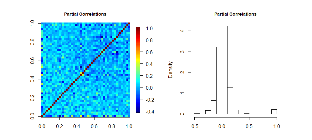
Since our interest is in constructing weights for the forecast combination, our goal is to estimate a precision matrix of the forecast errors. However, as pointed out by Koike, 2020, when common factors are present across the forecast errors, the precision matrix cannot be sparse because all pairs of the forecast errors are partially correlated given other forecast errors through the common factors. To illustrate this point, we generated forecast errors that follow (3.1) with $q=2$ and $\varepsilon_{t}\sim\mathcal{N}(\mathbf{0},{\bm{\Sigma}}_{\varepsilon})$, where $\sigma_{\varepsilon,ij}=0.4^{\left\lvert i-j\right\rvert}$ is the $i,j$-th element of ${\bm{\Sigma}}_{\varepsilon}$. The vector of factors ${\mathbf{f}}_{t}$ is drawn from $\mathcal{N}(\mathbf{0},{\mathbf{I}}_{q}/10)$, and the entries of the matrix of factor loadings for forecast error $j=1,\ldots,p$, ${\mathbf{b}}_{j}$, are drawn from $\mathcal{N}(\mathbf{0},{\mathbf{I}}_{q}/100)$. The full loading matrix is given by ${\mathbf{B}}=({\mathbf{b}}_{1},\ldots,{\mathbf{b}}_{p})^{\prime}$. Let $\widehat{q}$ denote the number of factors estimated by the PCA. We set $(T,p)=(1000,50)$ and plot the heatmap and histogram of population partial correlations of forecast errors ${\mathbf{e}}_{t}$, which are the entries of a precision matrix, in Figure 2. We now examine the performance of graphical models for estimating partial correlations under the factor structure. Figure 3 shows the partial correlations estimated by GLASSO that does not take into account factors: due to strict sparsity imposed by graphical models almost all partial correlations are shrunk to zero which degenerates the histogram in Figure 3. This means that strong sparsity assumption on ${\bm{\Theta}}$ imposed by classical graphical models (such as GLASSO and nodewise regression from Algorithms 1-2) is not realistic under the factor structure.

In order to avoid the aforementioned problem, instead of imposing sparsity assumption on the precision of forecast errors, ${\bm{\Theta}}$, we require sparsity of the precision matrix of the idiosyncratic errors, ${\bm{\Theta}}_{\varepsilon}$. The latter is obtained using the estimated residuals after removing the co-movements induced by the factors (see Barigozzi et al., 2018; Brownlees et al., 2018; Koike, 2020). Naturally, once we condition on the common components, it is sensible to assume that many remaining partial correlations of ${\bm{\varepsilon}}_{t}$ will be negligible and thus ${\bm{\Theta}}_{\varepsilon}$ is sparse.

We use the weighted Graphical Lasso and nodewise regression as shrinkage techniques to estimate the precision matrix of residuals. Once the precision of the low-rank component is obtained, we use the Sherman-Morrison-Woodbury formula to estimate the precision of forecast errors:

To obtain $\widehat{{\bm{\Theta}}}_{f}=\widehat{{\bm{\Sigma}}}_{f}^{-1}$, we use $\widehat{{\bm{\Sigma}}}_{f}=\frac{1}{T}\sum_{t=1}^{T}\widehat{{\mathbf{f}}}_{t}\widehat{{\mathbf{f}}}_{t}^{{}^{\prime}}$. To get $\widehat{{\bm{\Theta}}}_{\varepsilon}$, we develop two approaches: the first uses the weighted GLASSO Algorithm 1, with the initial estimate of the covariance matrix of the idiosyncratic errors calculated as $\widehat{{\bm{\Sigma}}}_{\varepsilon}=\frac{1}{T}\sum_{t=1}^{T}\widehat{{\bm{\varepsilon}}}_{t}\widehat{{\bm{\varepsilon}}}_{t}^{{}^{\prime}}$, where $\widehat{{\bm{\varepsilon}}}_{t}={\mathbf{e}}_{t}-\widehat{{\mathbf{B}}}\widehat{{\mathbf{f}}}_{t}$. The second uses nodewise regression and applies Algorithm 2 to $\widehat{{\bm{\varepsilon}}}_{t}$. Once we estimate $\widehat{{\bm{\Theta}}}_{f}$ and $\widehat{{\bm{\Theta}}}_{\varepsilon}$, we can get $\widehat{{\bm{\Theta}}}$ using a sample analogue of (4.1). We call the proposed procedures Factor Graphical Lasso and Factor nodewise regression and summarize them in Algorithm 3 and Algorithm 4 respectively.

Note that Algorithms 3 and 4 involve the tuning parameters $\lambda$ and $\lambda_{j}$, the procedure on how to choose the shrinkage intensity coefficients is described in more detail in Subsection 4.1 that describes how to choose the shrinkage intensity in practice, and Section 5 that establishes sparsity requirements that guarantee convergence of (4.2), (4.3), (4.4), and (4.5).

We can use $\widehat{{\bm{\Theta}}}$ to estimate the forecast combination weights $\widehat{{\mathbf{w}}}$

where $\widehat{{\bm{\Theta}}}$ is obtained from Algorithm 3 or Algorithm 4. Let us now revisit the motivating example at the beginning of this section: Figures 4-6 plot the heatmaps and the estimated partial correlations when precision matrix is computed using Factor GLASSO in Algorithm 3 with $\widehat{q}\in\{1,2,3\}$ statistical factors. The heatmaps and histograms closely resemble population counterparts in Figure 2, and the result is not very sensitive to over- or under-estimating the number of factors $\widehat{q}$. This demonstrates that using a combination of classical graphical models and factor structure via Factor Graphical Models in Algorithms 3-4 improves upon the performance of classical graphical models: our approach allows to extract the benefits of modeling common movements in forecast errors, captured by a factor model, and the benefits of using many competing forecasting models that give rise to a high-dimensional precision matrix, captured by a graphical model.

We first introduce some terminology and notations. Let $A\in\mathcal{S}_{p}$. Define the following set for $j=1,\ldots,p$:

where $d_{j}(A)$ is the number of edges adjacent to the vertex $j$ (i.e., the degree of vertex $j$), and $d(A)$ measures the maximum vertex degree. Define $S(A)\equiv\bigcup_{j=1}^{p}D_{j}(A)$ to be the overall off-diagonal sparsity pattern, and $s(A)\equiv\sum_{j=1}^{p}d_{j}(A)$ is the overall number of edges contained in the graph. Note that $\text{card}(S(A))\leq s(A)$: when $s(A)=p(p-1)/2$ this would give a fully connected graph.

For the nodewise regression in (4.4), denote $D_{j}\equiv\{k;\gamma_{j,k}\neq 0\}$ to be the active set for row ${\bm{\gamma}}_{j}$, and let $d_{j}\equiv\left\lvert D_{j}\right\rvert$. Define $\bar{d}\equiv\max_{1\leq j\leq p}d_{j}$.

We divide the simulation results into two subsections. In the first subsection we study the consistency of the Factor GLASSO and Factor MB for estimating precision matrix and the combination weights. In the second subsection we evaluate the out-of-sample forecasting performance of combined forecasts based on the Factor Graphical models from Algorithms 3-4 in terms of the mean-squared forecast error. We compare the performance of forecast combinations based on the factor models with equal-weighted (EW) forecast combination, forecast combinations using GLASSO and nodewise regression from Algorithms 1-2. Similarly to the literature on graphical models, all exercises use 100 Monte Carlo simulations.

References

- Bai, (2003) Bai, J. (2003). Inferential theory for factor models of large dimensions. Econometrica, 71(1):135–171.
- Bai and Ng, (2002) Bai, J. and Ng, S. (2002). Determining the number of factors in approximate factor models. Econometrica, 70(1):191–221.
- Barigozzi et al., (2018) Barigozzi, M., Brownlees, C., and Lugosi, G. (2018). Power-law partial correlation network models. Electronic Journal of Statistics, 12(2):2905–2929.
- Bates and Granger, (1969) Bates, J. M. and Granger, C. W. J. (1969). The combination of forecasts. Operations Research, 20(4):451–468.
- Brownlees et al., (2018) Brownlees, C., Nualart, E., and Sun, Y. (2018). Realized networks. Journal of Applied Econometrics, 33(7):986–1006.
- Cai et al., (2016) Cai, T. T., Liu, W., Zhou, H. H., et al. (2016). Estimating sparse precision matrix: Optimal rates of convergence and adaptive estimation. Annals of Statistics, 44(2):455–488.
- Callot et al., (2019) Callot, L., Caner, M., Önder, A. O., and Ulaşan, E. (2019). A nodewise regression approach to estimating large portfolios. Journal of Business & Economic Statistics, 0(0):1–12.
- Callot et al., (2017) Callot, L. A. F., Kock, A. B., and Medeiros, M. C. (2017). Modeling and forecasting large realized covariance matrices and portfolio choice. Journal of Applied Econometrics, 32(1):140–158.
- Chamberlain and Rothschild, (1983) Chamberlain, G. and Rothschild, M. (1983). Arbitrage, factor structure, and mean-variance analysis on large asset markets. Econometrica, 51(5):1281–1304.
- Chan et al., (1999) Chan, Y. L., Stock, J. H., and Watson, M. W. (1999). A dynamic factor model framework for forecast combination. Spanish Economic Review, 1(2):91–121.
- Chen and Chen, (2008) Chen, J. and Chen, Z. (2008). Extended bayesian information criteria for model selection with large model spaces. Biometrika, 95(3):759–771.
- Clemen, (1989) Clemen, R. T. (1989). Combining forecasts: A review and annotated bibliography. International Journal of Forecasting, 5(4):559–583.
- Connor and Korajczyk, (1988) Connor, G. and Korajczyk, R. A. (1988). Risk and return in an equilibrium APT: application of a new test methodology. Journal of Financial Economics, 21(2):255–289.
- Coulombe et al., (2020) Coulombe, P. G., Leroux, M., Stevanovic, D., and Surprenant, S. (2020). How is machine learning useful for macroeconomic forecasting? arXiv:2008.12477.
- Diebold and Shin, (2019) Diebold, F. and Shin, M. (2019). Machine learning for regularized survey forecast combination: Partially-egalitarian lasso and its derivatives. International Journal of Forecasting, 35(4):1679–1691.
- Fan et al., (2018) Fan, J., Liu, H., and Wang, W. (2018). Large covariance estimation through elliptical factor models. The Annals of Statistics, 46(4):1383–1414.
- Foygel and Drton, (2010) Foygel, R. and Drton, M. (2010). Extended bayesian information criteria for gaussian graphical models. In Proceedings of the 23rd International Conference on Neural Information Processing Systems - Volume 1, NIPS, pages 604–612, USA. Curran Associates Inc.
- Friedman et al., (2008) Friedman, J., Hastie, T., and Tibshirani, R. (2008). Sparse inverse covariance estimation with the Graphical Lasso. Biostatistics, 9(3):432–441.
- Hansen, (2008) Hansen, B. E. (2008). Least-squares forecast averaging. Journal of Econometrics, 146(2):342–350.
- Hautsch et al., (2012) Hautsch, N., Kyj, L. M., and Oomen, R. (2012). A blocking and regularization approach to high-dimensional realized covariance estimation. Journal of Applied Econometrics, 27(4):625–645.
- Janková and van de Geer, (2018) Janková, J. and van de Geer, S. (2018). Inference in high-dimensional graphical models. Handbook of Graphical Models, Chapter 14, pages 325–351. CRC Press.
- Koike, (2020) Koike, Y. (2020). De-biased graphical lasso for high-frequency data. Entropy, 22(4):456.
- Ledoit and Wolf, (2004) Ledoit, O. and Wolf, M. (2004). A well-conditioned estimator for large-dimensional covariance matrices. Journal of Multivariate Analysis, 88(2):365–411.
- Lee and Seregina, (2020) Lee, T.-H. and Seregina, E. (2020). Optimal portfolio using factor graphical lasso. arXiv:2011.00435.
- Liu et al., (2010) Liu, H., Roeder, K., and Wasserman, L. (2010). Stability approach to regularization selection (stars) for high dimensional graphical models. In Proceedings of the 23rd International Conference on Neural Information Processing Systems - Volume 2, NIPS’10, pages 1432–1440, USA. Curran Associates Inc.
- McCracken and Ng, (2016) McCracken, M. W. and Ng, S. (2016). FRED-MD: A monthly database for macroeconomic research. Journal of Business & Economic Statistics, 34(4):574–589.
- Meinshausen and Bühlmann, (2006) Meinshausen, N. and Bühlmann, P. (2006). High-dimensional graphs and variable selection with the Lasso. The Annals of Statistics, 34(3):1436–1462.
- Meinshausen and Bühlmann, (2010) Meinshausen, N. and Bühlmann, P. (2010). Stability selection. Journal of the Royal Statistical Society, Series B, 72:417–473.
- Seregina, (2020) Seregina, E. (2020). A basket half full: Sparse portfolios. arXiv preprint arXiv:2011.04278.
- Smith and Wallis, (2009) Smith, J. and Wallis, K. F. (2009). A simple explanation of the forecast combination puzzle. Oxford Bulletin of Economics and Statistics, 71(3):331–355.
- Stock and Watson, (2002) Stock, J. H. and Watson, M. W. (2002). Forecasting using principal components from a large number of predictors. Journal of the American Statistical Association, 97(460):1167–1179.
- van de Geer et al., (2014) van de Geer, S., Buhlmann, P., Ritov, Y., and Dezeure, R. (2014). On asymptotically optimal confidence regions and tests for high-dimensional models. The Annals of Statistics, 42(3):1166–1202.
- Zhao et al., (2012) Zhao, T., Liu, H., Roeder, K., Lafferty, J., and Wasserman, L. (2012). The HUGE package for high-dimensional undirected graph estimation in R. Journal of Machine Learning Research, 13(1):1059–1062.
- Zhu and Cribben, (2018) Zhu, Y. and Cribben, I. (2018). Sparse graphical models for functional connectivity networks: Best methods and the autocorrelation issue. Brain Connectivity, 8(3):139–165. PMID: 29634321.