Simulating Exceptional Non-Hermitian Metals with Single-Photon Interferometry
Abstract
We experimentally simulate in a photonic setting non-Hermitian (NH) metals characterized by the topological properties of their nodal band structures. Implementing nonunitary time evolution in reciprocal space followed by interferometric measurements, we probe the complex eigenenergies of the corresponding NH Bloch Hamiltonians, and study in detail the topology of their exceptional lines (ELs), the NH counterpart of nodal lines in Hermitian systems. We focus on two distinct types of NH metals: two-dimensional systems with symmetry-protected ELs, and three-dimensional systems possessing symmetry-independent topological ELs in the form of knots. While both types feature open Fermi surfaces, we experimentally observe their distinctions by analyzing the impact of symmetry-breaking perturbations on the topology of ELs.
Introduction.— Phases of quantum matter characterized by topologically robust nodal band structures, such as Weyl semimetals exhibiting remarkable transport properties Armitage et al. 2018, have been a major focus of both theoretical and experimental study for the past decade Armitage et al. 2018; Hasan and Kane 2010; Qi and Zhang 2011; Wehling et al. 2014; Ozawa et al. 2019; Bergholtz et al. 2021. Recently, it has become clear that non-Hermiticity, a common element in open, dissipative systems Bender and Boettcher 1998; Bender et al. 2002; Bender 2007; El-Ganainy et al. 2018, can qualitatively modify key features of band topology (see Ref. Bergholtz et al. 2021 for a review). This leads to a variety of fascinating phenomena, including the emergence of anomalous topological edge states Lee 2016; Xiao et al. 2017; Kunst et al. 2018; Xiong 2018; Yao and Wang 2018; Xiao et al. 2020a; Okuma et al. 2020; Zhang et al. 2021, and the presence of exceptional lines (ELs) Zhang et al. 2019, the non-Hermitian (NH) generalization of nodal lines along which the NH Hamiltonian is nondiagonalizable Xu et al. 2017; Molina and González 2018; Carlström and Bergholtz 2018; Budich et al. 2019; Carlström et al. 2019; Yang and Hu 2019; Wang et al. 2019a; Kawabata et al. 2019; Yang et al. 2020; Lee et al. 2020; Banerjee and Narayan 2020. In particular, at least two distinct classes of NH metals have been theoretically identified, one with ELs protected by NH symmetries that reduce the codimension of exceptional points (EPs) Budich et al. 2019; Yoshida et al. 2019, the other featuring nodal band structures and knotted ELs with intrinsic, symmetry-independent topology Carlström et al. 2019. These NH metals are in sharp contrast to their Hermitian, semimetal counterparts, where ELs and Fermi surfaces are reduced to isolated Weyl points and surface Fermi arcs, respectively Fang et al. 2016; Bi et al. 2017; Ezawa 2017; Türker and Moroz 2018; Zhou et al. 2018. While nodal band structures in both Hermitian and NH settings have seen a great surge of experimental interest recently Bzdušek et al. 2016; Yan et al. 2018; Song et al. 2019; Zhou et al. 2019; Xiao et al. 2020b; Chen et al. 2020, a systematic study of unconventional NH metals and their topological stability is still lacking.

In this work, we experimentally simulate and observe NH metals using single-photon interferometry (see Fig. 1 for an illustration of our setup), with a particular focus on the stability and topology of the ELs with respect to perturbations. Experimentally, this is achieved by implementing nonunitary time evolution for single photons that is governed by a corresponding NH Hamiltonian, and by performing interferometric measurements on the photons to extract the complex eigenenergies for each mode in reciprocal space. We simulate both NH metals featuring symmetry-protected ELs in two-dimensional (2D) systems and knotted ELs including a trefoil knot in three-dimensional (3D) systems, thus observing how EPs may form closed lines and even knots in momentum space.
More specifically, for symmetry-protected NH models in 2D, we show that the closed exceptional-line structures bound open Fermi volumes, and are robust against symmetry-preserving perturbations, while symmetry-breaking terms generically remove the ELs. This is in contrast to their 2D Hermitian analogs, where nodal points occur only at isolated momenta and do not give rise to bulk Fermi volumes. We further simulate 3D NH metals with both knotted and linked ELs that bound open Fermi surfaces representing the topological Seifert-surfaces of the corresponding knots Carlström et al. 2019. There, observing the robustness of the band-structure topology with respect to generic perturbations, we confirm the topological stability of nodal knots in NH systems. Our results thus experimentally establish the topological variety and stability of nodal structures in NH metals.
Theoretical framework.— We consider two-band NH metals, as described in reciprocal space by the NH Bloch Hamiltonian
| (1) |
where are the standard Pauli matrices, k is the lattice momentum for either a 2D or 3D lattice model, with the complex Bloch vector , where . With the eigenvalues of the NH Bloch Hamiltonian (1) given by , EPs occur whenever eigenvalues coalesce () at nonvanishing d, i.e., for nontrivial solutions to the equations and Miri and Alú 2019. Depending on the presence of NH symmetries as well as the spatial dimension of the system, the EPs can form closed ELs in the reciprocal space, with either symmetry-protected, or symmetry-independent topology. Specifically, ELs independent of symmetry occur in 3D, while suitable NH symmetries may reduce the codimension of EPs by one, thus stabilizing ELs in 2D systems. In both cases, ELs constitute boundaries for open Fermi volumes or surfaces, characterized by vanishing real parts of the energy gap, thus giving rise to symmetry-protected or intrinsic NH metals. Besides their topological stability, ELs in 3D may be topologically distinguished by forming different knots Carlström et al. 2019.
For the symmetry-protected NH metal, we consider a model on a 2D square lattice with unit lattice constant preserving the NH symmetry
| (2) |
By taking , the relation is satisfied automatically Budich et al. 2019. The ELs are therefore defined and tunable as closed contours in 2D momentum space that satisfy the single constraint . In particular, the parameter space is divided into regions with entirely real and entirely imaginary eigenspectrum, with ELs forming the boundary between the two.
By contrast, in three dimensions, the solutions of and each yield a closed 2D surface in 3D momentum space, and these two hyperplanes generically intersect at topologically stable closed lines in the parameter space, thus giving rise to NH metals with ELs that are robust against symmetry-breaking perturbations. These ELs with intrinsic topology can form knots or links in reciprocal space, and are thus fundamentally distinct from symmetry-protected ELs in 2D.
Experimental simulations.— We observe both symmetry-protected and intrinsic ELs by simulating the corresponding NH Bloch Hamiltonians in reciprocal space, and by measuring the complex eigenenergies using single-photon interferometry. While an arbitrary NH dynamic is difficult to implement experimentally due to the difficulty of achieving gain in quantum systems Weimann et al. 2017, especially with single photons, we circumvent this difficulty through a mapping
| (3) |
where is the identity matrix, and , with and the eigenvalue of Halmos 1950; Sparrow et al. 2018. It follows that and have the same eigenstates, while eigenenergies of are related to those of through .
As a general framework, we encode the basis states into the orthogonal polarization states of a single photon, and initialize the polarization state in , the eigenstates of of a given sector. We then send the photon through a beam splitter, after which the photon is in the state
| (4) |
where and denote the transmitted and reflected modes of the single photon, respectively. The nonunitary time evolution governed by is selectively enforced on the transmitted photon, leading to the state
| (5) |
from which is extracted through an interferometric measurement SM.
Symmetry-protected ELs.— We first simulate the following 2D NH Hamiltonian with symmetry-protected ELs
| (6) |
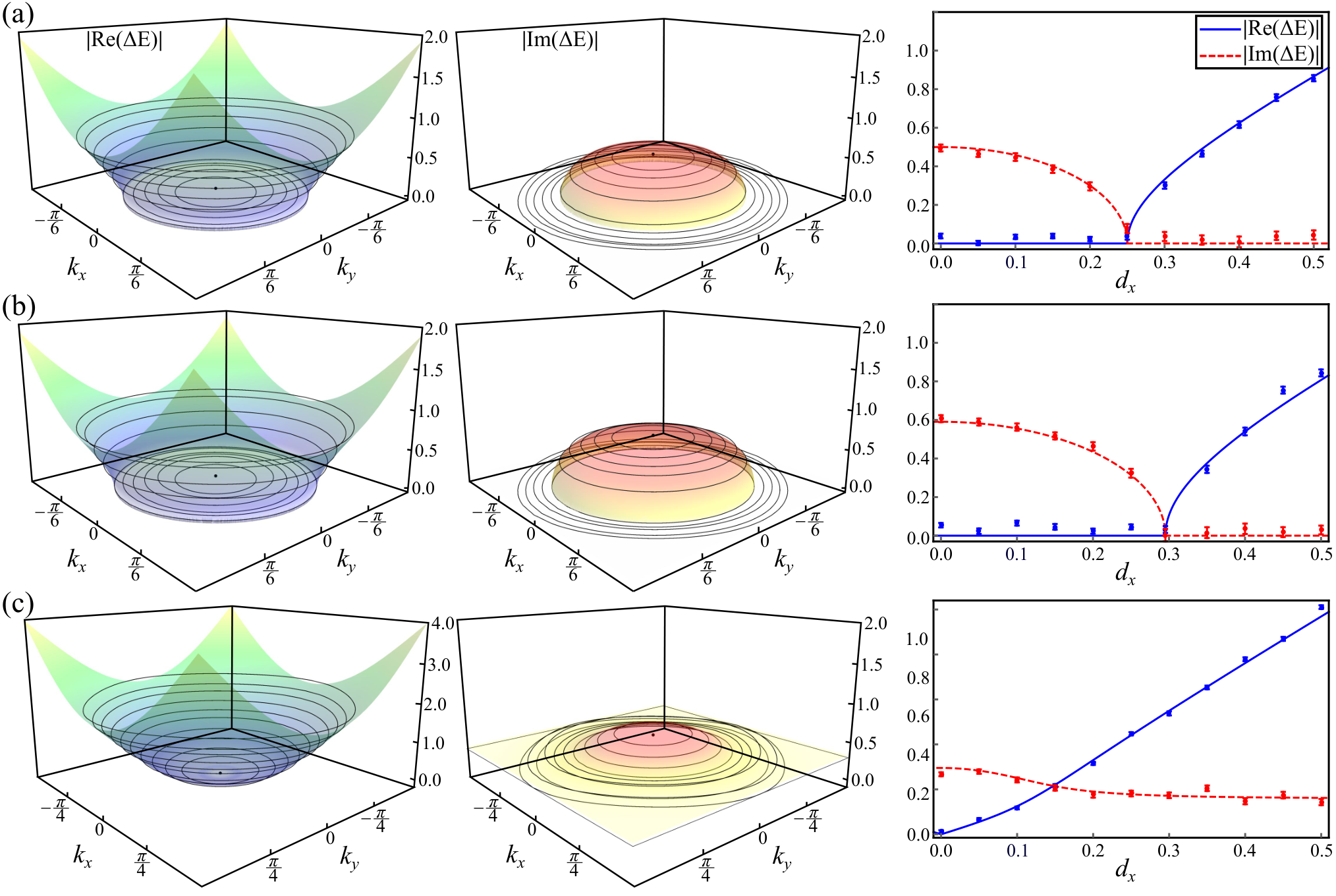
Note that satisfies the symmetry defined in Eq. (2). We sample different Bloch vectors , and measure the eigenenergies of both bands. Each sampled corresponds to a closed loop in the Brillouin zone that has the same eigenenergy. In Fig. 2(a), we show the real and imaginary components of the energy gap in momentum space, which agree well with theoretical predictions. Particularly, an exceptional ring exists at , by which the parameter space is divided into regions with either real or purely imaginary eigenenergies. It follows that the exceptional ring serves as a boundary for the open Fermi volume with , i.e., an open set with the same dimensionality as the bulk system. As a defining signature of symmetry protection, the topology of the exceptional ring is robust against symmetry-preserving perturbations. This is illustrated in Fig. 2(b), where the exceptional ring persists but is shifted in parameter space (now at ), upon the addition of a small perturbative term of the form . By contrast, when a symmetry-breaking perturbation of the form is added [see Fig. 2(c)], EPs disappear, in accordance with theoretical predictions. Generalizing this strategy, we are able to experimentally simulate the general class of NH models with symmetry-protected ELs SM.


Symmetry-independent knotted ELs.— We now turn to NH models with symmetry-independent ELs. Following Ref. Carlström et al. 2019, we construct models with intrinsic knotted or linked ELs in momentum space. This is achieved by taking
| (7) |
in Eq. (1), where are real and continuous scalar functions constrained by , with and . Here, is a constant with sufficiently large amplitude, which is fixed as for our work. By construction, if are coprime (both even) integers, a NH Hamiltonian with Bloch vectors satisfying Eq. (7) features ELs with knot (link) topology.
For our experiment, we adopt the construction
| (8) | ||||
to generate the functions and (such a construction is not unique though). First, we solve and using , and simulate the corresponding NH Hamiltonian with trefoil-knotted ELs [see Fig. 3(a)]. In Figs. 3(b) and 3(c), we show the measured and with fixed (b) and (c) as functions of and , which agree well with the corresponding theoretical values and reveal the underlying knotted topology of the ELs. In this case, the knotted ELs serve as the boundary for the topologically nontrivial open Fermi-Seifert surface defined by Carlström et al. 2019.
To investigate the robustness of ELs, we introduce a general, symmetry-breaking perturbation , where are chosen randomly. The experimental data shown in Figs. 3(d)–3(f) corresponds to the coefficients , , and . With the addition of perturbations, the knotted ELs still exist [see Figs. 3(d)–3(f)], while their shapes are slightly deformed compared to those without perturbations. These observations experimentally confirm and exemplify the robustness of knotted ELs to generic perturbations.
As a second case of NH model with intrinsic ELs, we adopt the same construction (8), but with . The resulting NH Hamiltonian features ELs with a link geometry [see Fig. 4(a)]. The experimentally measured and with are shown in Figs. 4(b) and 4(c). Similar to the knotted ELs, the linked topology here is also found to be robust to generic perturbations.
Conclusion.— By simulating and observing two different classes of NH metals, our present experimental study corroborates the topological robustness of ELs that occur in a rich variety of nodal NH band structures. While our findings hopefully inspire the investigation of exotic NH metals also in other physical platforms, we note that our present experimental scheme may readily be extended to multiband models and systems with other symmetries, thus offering a versatile toolbox for the systematic experimental study of nodal phases in both Hermitian and non-Hermitian settings. Furthermore, our configuration enables the investigation of dynamical properties of NH metals, where the presence of open Fermi volumes or open Fermi surfaces may give rise to so far unexplored phenomena.
Acknowledgements.
We acknowledge fruitful discussions with Emil J. Bergholtz. This work has been supported by the Natural Science Foundation of China (Grants No. 12025401, No. 11974331, and No. U1930402). L. X. acknowledges support from the project funded by China Postdoctoral Science Foundation (Grant No. 2020M680006). W. Y. acknowledges support from the National Key Research and Development Program of China (Grants No. 2016YFA0301700 and No. 2017YFA0304100). J. C. B. acknowledges financial support from the German Research Foundation (DFG) through the Collaborative Research Centre SFB 1143 (project ID 247310070) and the Cluster of Excellence ct.qmat (EXC 2147, project ID 390858490).References
- Armitage et al. (2018) N. P. Armitage, E. J. Mele, and A. Vishwanath, “Weyl and Dirac semimetals in three-dimensional solids,” Rev. Mod. Phys. 90, 015001 (2018).
- Hasan and Kane (2010) M. Z. Hasan and C. L. Kane, “Topological insulators,” Rev. Mod. Phys. 82, 3045 (2010).
- Qi and Zhang (2011) X.-L. Qi and S.-C. Zhang, “Topological insulators and superconductors,” Rev. Mod. Phys. 83, 1057 (2011).
- Wehling et al. (2014) T. O. Wehling, A. M. Black-Schaffer, and A. V. Balatsky, “Dirac materials,” Adv. Phys. 63, 1–76 (2014).
- Ozawa et al. (2019) T. Ozawa, H. M. Price, A. Amo, N. Goldman, M. Hafezi, L. Lu, M. C. Rechtsman, D. Schuster, J. Simon, O. Zilberberg, and I. Carusotto, “Topological photonics,” Rev. Mod. Phys. 91, 015006 (2019).
- Bergholtz et al. (2021) E. J. Bergholtz, J. C. Budich, and F. K. Kunst, “Exceptional topology of non-Hermitian systems,” Rev. Mod. Phys. 93, 015005 (2021).
- Bender and Boettcher (1998) C. M. Bender and S. Boettcher, “Real spectra in non-Hermitian Hamiltonians having symmetry,” Phys. Rev. Lett. 80, 5243 (1998).
- Bender et al. (2002) C. M. Bender, D. C. Brody, and H. F. Jones, “Complex extension of quantum mechanics,” Phys. Rev. Lett. 89, 270401 (2002).
- Bender (2007) C. M. Bender, “Making sense of non-Hermitian Hamiltonians,” Rep. Prog. Phys. 70, 947 (2007).
- El-Ganainy et al. (2018) R. El-Ganainy, K. G. Makris, M. Khajavikhan, Z. H. Musslimani, S. Rotter, and D. N. Christodoulides, “Non-Hermitian physics and symmetry,” Nat. Phys. 14, 11–19 (2018).
- Lee (2016) T. E. Lee, “Anomalous edge state in a non-Hermitian lattice,” Phys. Rev. Lett. 116, 133903 (2016).
- Xiao et al. (2017) L. Xiao, X. Zhan, Z. H. Bian, K. K. Wang, X. Zhang, X. P. Wang, J. Li, K. Mochizuki, D. Kim, N. Kawakami, W. Yi, H. Obuse, B. C. Sanders, and P. Xue, “Observation of topological edge states in parity–time-symmetric quantum walks,” Nat. Phys. 13, 1117–1123 (2017).
- Kunst et al. (2018) F. K. Kunst, E. Edvardsson, J. C. Budich, and E. J. Bergholtz, “Biorthogonal bulk-boundary correspondence in non-Hermitian systems,” Phys. Rev. Lett. 121, 026808 (2018).
- Xiong (2018) Y. Xiong, “Why does bulk boundary correspondence fail in some non-Hermitian topological models,” J. Phys. Commun. 2, 035043 (2018).
- Yao and Wang (2018) S. Yao and Z. Wang, “Edge states and topological invariants of non-Hermitian systems,” Phys. Rev. Lett. 121, 086803 (2018).
- Xiao et al. (2020a) L. Xiao, T. Deng, K. Wang, G. Zhu, Z. Wang, W. Yi, and P. Xue, “Non-Hermitian bulk-boundary correspondence in quantum dynamics,” Nat. Phys. 16, 761–766 (2020a).
- Okuma et al. (2020) N. Okuma, K. Kawabata, K. Shiozaki, and M. Sato, “Topological origin of non-Hermitian skin effects,” Phys. Rev. Lett. 124, 086801 (2020).
- Zhang et al. (2021) X. Zhang, G. J. Li, Y. H. Liu, T. Tai, R. Thomale, and C. H. Lee, “Tidal surface states as fingerprints of non-Hermitian nodal knot metals,” Commun. Phys. 4, 47 (2021).
- Zhang et al. (2019) X. Zhang, K. Ding, X. Zhou, J. Xu, and D. Jin, “Experimental observation of an exceptional surface in synthetic dimensions with magnon polaritons,” Phys. Rev. Lett. 123, 237202 (2019).
- Xu et al. (2017) Y. Xu, S.-T. Wang, and L.-M. Duan, “Weyl exceptional rings in a three-dimensional dissipative cold atomic gas,” Phys. Rev. Lett. 118, 045701 (2017).
- Molina and González (2018) R. A. Molina and J. González, “Surface and 3D quantum Hall effects from engineering of exceptional points in nodal-line semimetals,” Phys. Rev. Lett. 120, 146601 (2018).
- Carlström and Bergholtz (2018) J. Carlström and E. J. Bergholtz, “Exceptional links and twisted Fermi ribbons in non-Hermitian systems,” Phys. Rev. A 98, 042114 (2018).
- Budich et al. (2019) J. C. Budich, J. Carlström, F. K. Kunst, and E. J. Bergholtz, “Symmetry-protected nodal phases in non-Hermitian systems,” Phys. Rev. B 99, 041406(R) (2019).
- Carlström et al. (2019) J. Carlström, M. Stålhammar, J. C. Budich, and E. J. Bergholtz, “Knotted non-Hermitian metals,” Phys. Rev. B 99, 161115(R) (2019).
- Yang and Hu (2019) Z. Yang and J. Hu, “Non-Hermitian Hopf-link exceptional line semimetals,” Phys. Rev. B 99, 081102(R) (2019).
- Wang et al. (2019a) H. Wang, J. Ruan, and H. Zhang, “Non-Hermitian nodal-line semimetals with an anomalous bulk-boundary correspondence,” Phys. Rev. B 99, 075130 (2019a).
- Kawabata et al. (2019) K. Kawabata, T. Bessho, and M. Sato, “Classification of exceptional points and non-Hermitian topological semimetals,” Phys. Rev. Lett. 123, 066405 (2019).
- Yang et al. (2020) Z. Yang, C.-K. Chiu, C. Fang, and J. Hu, “Jones polynomial and knot transitions in Hermitian and non-Hermitian topological semimetals,” Phys. Rev. Lett. 124, 186402 (2020).
- Lee et al. (2020) C. H. Lee, A. Sutrisno, T. Hofmann, T. Helbig, Y. Liu, Y. S. Ang, L. K. Ang, X. Zhang, M. Greiter, and R. Thomale, “Imaging nodal knots in momentum space through topolectrical circuits,” Nat. Commun. 11, 4385 (2020).
- Banerjee and Narayan (2020) A. Banerjee and A. Narayan, “Non-Hermitian semi-Dirac semi-metals,” arXiv:2001.11188 (2020).
- Yoshida et al. (2019) T. Yoshida, R. Peters, N. Kawakami, and Y. Hatsugai, “Symmetry-protected exceptional rings in two-dimensional correlated systems with chiral symmetry,” Phys. Rev. B 99, 121101(R) (2019).
- Fang et al. (2016) C. Fang, H. Weng, X. Dai, and Z. Fang, “Topological nodal line semimetals,” Chin. Phys. B 25, 117106 (2016).
- Bi et al. (2017) R. Bi, Z. Yan, L. Lu, and Z. Wang, “Nodal-knot semimetals,” Phys. Rev. B 96, 201305(R) (2017).
- Ezawa (2017) M. Ezawa, “Topological semimetals carrying arbitrary Hopf numbers: Fermi surface topologies of a Hopf link, Solomon’s knot, trefoil knot, and other linked nodal varieties,” Phys. Rev. B 96, 041202(R) (2017).
- Türker and Moroz (2018) O. Türker and S. Moroz, “Weyl nodal surfaces,” Phys. Rev. B 97, 075120 (2018).
- Zhou et al. (2018) H. Zhou, C. Peng, Y. Yoon, C. W. Hsu, K. A. Nelson, L. Fu, J. D. Joannopoulos, M. Soljaǔiú, and B. Zhen, “Observation of bulk Fermi arc and polarization half charge from paired exceptional points,” Science 359, 1009–1012 (2018).
- Bzdušek et al. (2016) T. Bzdušek, Q. S. Wu, A. Rüegg, M. Sigrist, and A. A. Soluyanov, “Nodal-chain metals,” Nature 538, 75–78 (2016).
- Yan et al. (2018) Q. Yan, R. Liu, Z. Yan, B. Liu, H. Chen, Z. Wang, and L. Lu, “Experimental discovery of nodal chains,” Nat. Phys. 14, 461–464 (2018).
- Song et al. (2019) B. Song, C. He, S. Niu, L. Zhang, Z. Ren, X.-J. Liu, and G.-B. Jo, “Observation of nodal-line semimetal with ultracold fermions in an optical lattice,” Nat. Phys. 15, 911–916 (2019).
- Zhou et al. (2019) H. Zhou, J. Y. Lee, S. Liu, and B. Zhen, “Exceptional surfaces in -symmetric non-Hermitian photonic systems,” Optica 6, 190–193 (2019).
- Xiao et al. (2020b) M. Xiao, L. Ye, C. Qiu, H. He, Z. Liu, and S. Fan, “Experimental demonstration of acoustic semimetal with topologically charged nodal surface,” Sci. Adv. 6, eaav2360 (2020b).
- Chen et al. (2020) M. Chen, C. Li, G. Palumbo, Y.-Q. Zhu, N. Goldman, and P. Cappellaro, “Experimental characterization of the 4D tensor monopole and topological nodal rings,” arXiv: 2008.00596 (2020).
- Miri and Alú (2019) M.-A. Miri and A. Alú, “Exceptional points in optics and photonics,” Science 363, eaar7709 (2019).
- Weimann et al. (2017) S. Weimann, M. Kremer, Y. Plotnik, Y. Lumer, S. Nolte, K. G. Makris, M. Segev, M. C. Rechtsman, and A. Szameit, “Topologically protected bound states in photonic parity–time-symmetric crystals,” Nat. Mater. 16, 433–438 (2017).
- Halmos (1950) P. R. Halmos, “Normal dilations and extensions of operators,” Summ. Bras. Math. 2, 125 (1950).
- Sparrow et al. (2018) C. Sparrow, E. Martin-Lopez, N. Maraviglia, A. Neville, C. Harrold, J. Carolan, Y. N. Joglekar, T. Hashimoto, N. Matsuda, J. L. O’Brien, D. P. Tew, and A. Laing, “Simulating the vibrational quantum dynamics of molecules using photonics,” Nature 557, 660–667 (2018).
- (47) See Supplemental Material at [URL will be inserted by publisher] for experimental details, alternative model with symmetry-protected exceptional lines, further information of intrinsic exceptional lines and robustness of exceptional lines against perturbation, which includes Refs. Xiao et al. 2019; Wang et al. 2019b; Wang et al. 2018; Gilchrist et al. 2005; Jamiolkowski 1972.
- Xiao et al. (2019) L. Xiao, K. K. Wang, X. Zhan, Z. H. Bian, K. Kawabata, M. Ueda, W. Yi, and P. Xue, “Observation of critical phenomena in parity–time-symmetric quantum dynamics,” Phys. Rev. Lett. 123, 230401 (2019).
- Wang et al. (2019b) K. K. Wang, X. Qiu, L. Xiao, X. Zhan, Z. H. Bian, W. Yi, and P. Xue, “Simulating dynamic quantum phase transitions in photonic quantum walks,” Phys. Rev. Lett. 122, 020501 (2019b).
- Wang et al. (2018) K. K. Wang, X. P. Wang, X. Zhan, Z. H. Bian, J. Li, B. C. Sanders, and P. Xue, “Entanglement-enhanced quantum metrology in a noisy environment,” Phys. Rev. A 97, 042112 (2018).
- Gilchrist et al. (2005) A. Gilchrist, N. K. Langford, and M. A. Nielsen, “Distance measures to compare real and ideal quantum processes,” Phys. Rev. A 71, 062310 (2005).
- Jamiolkowski (1972) A. Jamiolkowski, “Linear transformations which preserve trace and positive semidefiniteness of operators,” Rep. Math. Phys. 3, 275 (1972).
Appendix A SUPPLEMENTAL MATERIAL FOR “SIMULATING EXCEPTIONAL NON-HERMITIAN METALS WITH SINGLE-PHOTON INTERFEROMETRY”
A.1 Experimental detection
A qubit is encoded in the polarization of a single photon , generated by the standard spontaneous parametric down-conversion, and projected into the eigenstate of with a polarizing beam splitter (PBS), a half-wave plate (HWP) and a quarter-wave plate (QWP).
Following the beam splitter (BS), the photon state is given by
| (S1) |
where and denote the transmission and reflection modes of the single photons, respectively. To measure the complex phase shift under , we perform the nonunitary operation on the polarization state of the photons in the transmission mode and keep that in the reflected mode unchanged, i.e., , where is the identity operator. The nonunitary operation can be realized by an interferometric network involving beam displacers (BDs) and wave plates.
As illustrated in Fig. 1 of the main text, in our experiment we decompose according to Xiao et al. 2019, where an arbitrary rotation of () is realized by two QWPs and a HWP. Two BDs and two HWPs with setting angles and are used to realize the polarization-dependent loss operator , where is determined by the loss parameter of .
The state then evolves according to
| (S2) |
We then perform interferometric measurements Wang et al. 2019b: a HWP at is applied on the polarizations of the photons in the transmitted mode. After passing through a polarizing beam splitter (PBS), the state evolves into
| (S3) |
under the assumption that . Here () denotes the transmitted (reflected) mode following the second PBS in the path of the -mode photons. We perform projective measurements with the bases on the polarizations of the photons in either of the transmitted () or reflected () mode. The outputs are recorded in coincidence with trigger photons. The coincidences are denoted as , which satisfy the following relations
| (S4) |
where corresponds to the number of photons in mode. We then obtain through
| (S5) |
when the polarization of photons in the mode is measured. Similarly, when the polarization of the photons in the mode is measured, we have
| (S6) |
where is an integer. From the relation , one can also obtain the eigenenergies of .
Here we give a concrete example of our experimental process. For a 2D non-Hermitian Hamiltonian with symmetry-protected exceptional lines in Eq. (6) of the main text, with Bloch vector . The corresponding nonunitary evolution with unit time is then . Instead, in our experiment we realize the passive nonunitary operation governed by the effective Hamiltonian with . The heralded single photons are prepared in the state via a HWP at and a QWP at as the operators of HWPs and QWPs are and , respectively. The passive nonunitary operation is decomposed as , where , , and . To implement it, all the QWPs are set as and the HWPs are set at , and (from left to right, Fig. 1 in the main text), respectively.
To verify the accuracy of the nonunitary operation in our experiment, we adopt a quantity that characterizes the distance between the implemented and the target operations. In general, an operation in a quantum system can be expressed in the operator-sum representation as a positive-definite process matrix which relates the output state with the input state , through
| (S7) |
where are the elements of the process matrix , corresponds to the standard Pauli matrix in general dimensions, and stands for the quantum process. We then define a distance , with
| (S8) |
where and are, respectively, the measured process matrix via process tomography Wang et al. 2018 and its theoretical predictions. The distance varies between and , which can be used to quantify the match between the measured process matrix and its theoretical prediction Gilchrist et al. 2005, with indicating a perfect match and indicating a complete mismatch. For our experiments, we obtain , indicating an excellent match.
Alternatively, we may define the distance based on the Jamiolkowski isomorphism of a quantum process Jamiolkowski 1972
| (S9) |
where is the maximally entangled state of the system and a -dimensional ancilla ( is the dimension of the system), and is the computational basis. The distance between the measured and ideal processes can be quantified using the trace distance
| (S10) |
where and are, respectively, the state obtained via the process tomography and its theoretical prediction. It has been shown that serves as the upper bound on the distance between the measured and ideal joint probability distributions during a sampling computation Gilchrist et al. 2005. For our experiments, we obtain , again indicating an excellent match.
A.2 Alternative model with symmetry-protected exceptional lines

As a complement to in the main text, we consider an alternative 2D model with symmetry-protected exceptional lines
| (S11) |
where . Note that also satisfies the symmetry in Eq. (2) (in the main text) with . In Figs. S1(a) and (b), we choose , satisfying the condition . We then sample sectors in the Brillouin zone (dots in Fig. S1), with , , and , . By observing the behavior of and (see Fig. S2), we are able to infer the locations of exceptional points, which form a pair of closed loops in the momentum space, consistent with theoretical predictions. The closed exceptional lines form the boundary for open 2D Fermi surfaces.
Similarly, in Figs. S1(c) and (d) [see also Fig. S3], we choose , satisfying . We then sample the Brillouin zone: , , and , . The inner exceptional line in this case collapses into a single exceptional point. Further increase in [see Figs. S1(e) and (f); see also Fig. S4] leads to the splitting of the outer exceptional line into four Fermi pockets. Finally, for sufficiently large [see Figs. S1(g) and (h); see also Fig. S5], all four exceptional lines collapse to four exceptional points. We have checked that the existence of exceptional lines or exceptional points are also robust against symmetry-preserving perturbations.
A.3 Further information of intrinsic exceptional lines

In Figs. S6 and S7, we provide cross-sectional view for experimental data points in Figs. 3 and 4 of the main text. Crucially, whereas eigenenergie can be significantly affected by perturbations, the topology of exceptional lines are unchanged.


A.4 Robustness of exceptional lines against perturbation
We now present a quantitative analysis regarding the robustness of exceptional lines against perturbation. First, we consider the case of symmetry-protected exceptional lines, under the non-Hermitian Hamiltonian in Eq. (6) of the main text. For , the exceptional lines are robust against a small symmetry-preserving perturbation of the form when is satisfied. The exceptional lines disappear for . Under the symmetry-preserving perturbations of and , the exceptional lines disappear for and , respectively. In our experiment, we choose , and , corresponding to the red, blue and green symbols in Fig. S8(a). As illustrated in Figs. S8(b-d), the exceptional lines disappear in accordance with theoretical predictions.
The second case we consider is the symmetry-independent knotted exceptional lines. Under a small perturbation with the form (, ), the knotted exceptional lines are still robust. However, with sufficiently large , the knotted exceptional lines disappear. We choose the exceptional point with and vary . The knotted exceptional lines disappear for , and , respectively. In our experiment, we choose , and , the knotted exceptional lines disappear in accordance with theoretical predictions as shown in Fig. S9.
Similarly, the symmetry-independent, linked exceptional lines are robust against small perturbation, but disappear when the strength of the perturbation increases, i.e., , and . In our experiment, we choose , and , the linked exceptional lines disappear in accordance with theoretical predictions as shown in Fig. S10.