On the Relevance-Complexity Region of Scalable Information BottleneckThanks: Thanks: The work of M. Kobayashi was supported by DFG.Thanks: 

In statistical (supervised) learning models, one seeks to strike a right balance between accuracy and generalization capability. Many existing machine learning algorithms generally fail to do so; or else only at the expense of large amounts of algorithmic components and hyperparameters that are heavily tuned heuristically for a given task (and, even so, generally fall short of generalizing to other tasks). The Information Bottleneck (IB) method [1], which is essentially a remote source coding problem under logarithmic loss fidelity measure, attempts to do so by finding a suitable tradeoff between algorithm’s robustness, measured by compression complexity, and accuracy or relevance, measured by the allowed average logarithmic loss (see e.g.  [2, 3]). More specifically, for a target (label) variable $X$ and an observed variable $Y$, the IB finds a description $U$ that is maximally informative about $X$ while being minimally informative about $Y$, where informativeness is measured via Shannon’s mutual information.

We study a variation of the IB problem, called scalable information bottleneck, where the encoder outputs $T\geq 2$ descriptions with increasingly richer features. This is motivated primarily by application scenarios in which a varying level of accuracy is required depending on the allowed and/or required level of complexity. The model is illustrated in Fig. 1 for the case of $T=2$. As an example, one may think about the simple scenario of making inference about a moving object on the road. A decision maker which receives only coarse information about the object would have to merely identify its type (e.g., car, bicycle, bus), while one that receives also refinement information would have to infer more accurate description, such as color, speed, and so on.

While a single-letter characterization of the optimal relevance-complexity region of this model can be found easily by specializing the result of [4, Theorem 1] to the case of logarithmic loss measure, we here establish explicit (analytic) characterizations of the relevance-complexity region for two examples, i.e. memoryless Gaussian and memoryless binary sources. Then, we derive a Blahut-Arimoto type algorithm that allows us to compute (an approximation of) the region for general discrete sources. Finally, we illustrate the usefulness of our results through an application example in the pattern classification problem.

The relevance-complexity tradeoff has been studied in various setups, including the distributed inference [5, 6], multivariate [7] and multi-layer [8] scenarios. Although multivariate IB [7] considers a more general setup, the coding method as well as the achievable relevance-complexity region have not been investigated. Notice that our model is conceptually different from the multi-layer IB [8] that considers non-identical hidden variables (sources) and the input of a given layer as the output of the previous layer.

Throughout this paper, we use the following notation. Upper and lower case letters are used to denote random variables and their realizations, e.g., $X$ and $x$, respectively while calligraphic letters, e.g., $\mathcal{X}$, denote sets. $X^{n}$ denotes $(X_{1},X_{2},\dots,X_{n})$ and $[K]=\{1,\dots,K\}$. We use $\mathcal{P(X)}$ to denote the set discrete probability distributions on $\mathcal{X}$. $H(X)$ denotes the entropy of a discrete random variable $X\in{\cal X}$ while $h(X)$ denotes the differential entropy of a continuous random variable. $h_{2}(p)\stackrel{{\scriptstyle\Delta}}{{=}}-p\log_{2}p-(1-p)\log_{2}(1-p)$ for $p\in[0,1/2]$ denotes the binary entropy function.

Let $(X^{n},Y^{n})\in{\cal X}^{n}\times{\cal Y}^{n}$ be a sequence of $n$ i.i.d. discrete random variables corresponding to the source and observation. An $\left(n,R_{1},\dots,R_{T}\right)$ successive refinement code for the $T$-scalable information bottleneck consists of

• •

  Encoding function $\phi_{t}^{(n)}:{\cal Y}^{n}\mapsto{\cal R}_{t}$ for $t=1,\dots,T$, where ${\cal R}_{t}=\left\{1,\dots,2^{nR_{t}}\right\}$.

• •

  Decoding function $\psi_{t}^{(n)}:{\cal R}_{1}\times\dots\times{\cal R}_{t}\mapsto\hat{{\cal X}}_{t}^{n}$, for $t=1,\dots,T$.

The decoder wishes to reconstruct the source in a scalable fashion, i.e. for $t=1,\dots,T$,

where $d(x,\hat{x})$ is a distortion function. In particular, we focus on the logarithmic distortion measure, given by $d_{\rm log}(x,\hat{x})=-\log(\hat{x}(x))$, where $\hat{x}(x)\in{\cal P}({\cal X})$ denotes the probability distribution (mass function) evaluated at $x\in{\cal X}$. We say that the rate-distortion tuples $(R_{1},\dots,R_{T},D_{1},\dots,D_{T})$ are achievable if there exists an $(n,R_{1},\dots,R_{T})$ $T$-scalable successive refinement code satisfying (1) for an arbitrarily large $n$. By letting $\Delta_{t}$ denote the relevance of stage-$t$ defined as $\Delta_{t}\stackrel{{\scriptstyle\Delta}}{{=}}H(X)-D_{t}$, the relevance-complexity region is defined as the minimum complexity (rate) tuple $(R_{1},\dots,R_{T})$ such that the relevance constraints $(\Delta_{1},\dots,\Delta_{T})$ are satisfied.

This section characterizes the relevance-complexity region of the $T$-scalable information bottleneck problem described in the previous section.

The rest of the section is dedicated to the converse proof as the achievability builds on the hierarchical random codes and successive decoding as described in [4].

In this Section, we propose a modified Blahut-Arimoto (BA) (see e.g. [11] algorithm which computes the region by iterating over a set of self-consistent equations when the source distribution is known or can be estimated with high accuracy. From the relevance-complexity region of (3), we wish to minimize the sum complexity under the individual relevance constraints.

We define the corresponding Lagrangian function as

where $\lambda(y)$ is the normalization term. By simple algebra, we readily obtain

where

and ${\cal T}_{\overline{l}}=[T]\setminus\{l\}$. Finally, our modified Blahut-Arimoto algorithm is summarized in Algorithm 1.

We conclude the paper by providing an application of the proposed scalable IB in the context of pattern classification. Consider the problem of classification in the proposed stucture shown in Fig. 1. In this problem, the role of the decoder is to guess the unknown class $X\in\mathcal{X}^{C}$, for the number of $C$ classes, on the basis of encoder outputs $U_{1},\dots,U_{T}$. Let $Q_{U^{T}|Y}$ be the encoder and $Q_{\hat{X}_{t}|U^{t}}$ be the soft-decoder output of stage $t\in[T]$. The pair of encoder and decoder induces a classifier at stage $t\in[T]$

where (a) follows because we have $Y-\!\!\!\!\minuso\!\!\!\!-U^{t}-\!\!\!\!\minuso\!\!\!\!-\hat{X}_{t}$. Following similar steps as [12, Section IV. C], we can show that the probability of classification error at stage $t$ of the $T$-scalable classiffer is given by

where (a) and (c) follows from Jensen’s inequality; (b) follows from (VI). By minimizing the average logarithmic loss in (VI), we obtain a tight lower bound on classification error probability. The minimum average logarithmic loss over all choices of decoders $Q_{\hat{X}_{t}|U^{t}}$ for any $t\in[T]$ and the encoder $Q_{U^{T}|Y}$ with rate no greater than $R_{t}$ bits per-sample in stage $t$ respectively, is $D_{t}^{*}=\inf\{D_{t}:(R_{1},\dots,R_{T},D_{1},\dots,D_{T})\in\mathcal{R}\}$, where $\mathcal{R}$ is the region stated in Theorem 1 and $t\in[T]$. Thus, we have

where the last equality follows from $\Delta_{t}^{*}=H(X)-D_{t}^{*}$, $t\in[T]$.

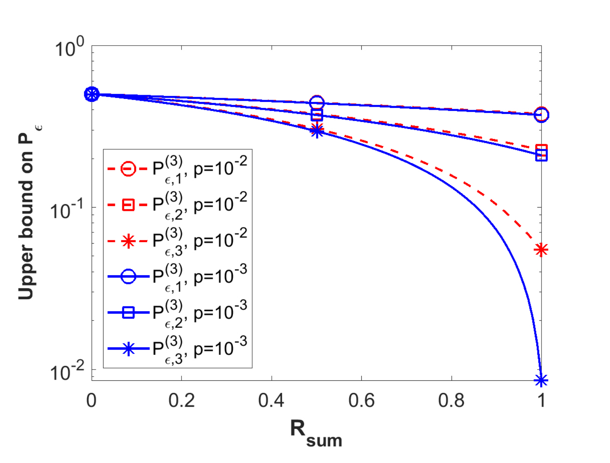
In Fig. 4, we evaluate the upper bound of the binary classification error probability for the case of $T=3$ and symmetric rate $R_{1}=R_{2}=R_{3}=R$, by combining (6) and (38). We can see that as the observation gets closer to the source (small $p$) the error probability smoothly decreases.

References

• [1] N. Tishby, F. C. Pereira, and W. Bialek, “The information bottleneck method,” in Proc. of the 37th Annu. Allerton Conf. Commun., Control and Comput. ACM, 1999.
• [2] A. Zaidi, I. Estella-Aguerri, and S. Shamai, “On the information bottleneck problems: Models, connections, applications and information theoretic views,” Entropy, vol. 22, no. 2, pp. 151, 2020.
• [3] Z. Goldfeld and Y. Polyanskiy, “The Information Bottleneck Problem and Its Applications in Machine Learning,” IEEE J. Sel. Topics Inf. Theory, 2020.
• [4] C. Tian and S. N. Diggavi, “On multistage successive refinement for Wyner–Ziv source coding with degraded side informations,” IEEE Trans. Inf. Theory, vol. 53, no. 8, pp. 2946–2960, 2007.
• [5] I. Estella-Aguerri and A. Zaidi, “Distributed information bottleneck method for discrete and Gaussian sources,” in International Zurich Seminar on Information and Communication (IZS 2018). Proceedings. ETH Zurich, 2018, pp. 35–39.
• [6] I. Estella-Aguerri and A. Zaidi, “Distributed Variational Representation Learning,” IEEE Transactions on Pattern Analysis and Machine Intelligence, 2019.
• [7] N. Friedman, O. Mosenzon, N. Slonim, and N. Tishby, “Multivariate information bottleneck,” Proc. Seventeenth Conf. on Uncertainty in Artificial Intelligence (UAI), 2001., 2001.
• [8] Q. Yang, P. Piantanida, and D. Gündüz, “The multi-layer information bottleneck problem,” in Proc. IEEE Inf. Theory Workshop (ITW). IEEE, 2017, pp. 404–408.
• [9] T. A. Courtade and T. Weissman, “Multiterminal source coding under logarithmic loss,” IEEE Trans. Inf. Theory, vol. 60, no. 1, pp. 740–761, 2013.
• [10] A. El Gamal and Y.-H. Kim, Network Information Theory, Cambridge University Press, 2011.
• [11] R. Blahut, “Computation of channel capacity and rate-distortion functions,” IEEE Trans. Inf. Theory, vol. 18, no. 4, pp. 460–473, 1972.
• [12] Y. Uğur, I. E. Aguerri, and A. Zaidi, “Vector Gaussian CEO Problem Under Logarithmic Loss and Applications,” IEEE Trans. Inf. Theory, vol. 66, no. 7, pp. 4183–4202, 2020.