跳到论文正文
W Papers独立论文阅读器 arXiv:2011.01338 论文正文 计算阅读时间 · 0%
引用这篇论文根据当前论文元数据生成,正式投稿前建议核对。


License: arXiv.org perpetual non-exclusive license
arXiv:2011.01338v2 [math.NA] 05 Nov 2020

The effect of quadrature rules on finite element solutions of Maxwell variational problems. Consistency estimates on meshes with straight and curved elements.Thanks: This work was supported in part by Fondecyt Regular 1171491 and doctoral grant Conicyt-PFCHA 2017-21171791.

Rubén Aylwin Affiliation: Department of Electrical Engineering, Pontificia Universidad Católica de Chile, Santiago, Chile.    Carlos Jerez-Hanckes Affiliation: Faculty of Engineering and Sciences, Universidad Adolfo Ibáñez, Santiago, Chile.
Abstract

We study the effects of numerical quadrature rules on error convergence rates when solving Maxwell-type variational problems via the curl-conforming or edge finite element method. A complete a priori error analysis for the case of bounded polygonal and curved domains with non-homogeneous coefficients is provided. We detail sufficient conditions with respect to mesh refinement and precision for the quadrature rules so as to guarantee convergence rates following that of exact numerical integration. On curved domains, we isolate the error contribution to numerical quadrature rules.

1 Introduction

We provide a complete error analysis on the effects of numerical integration when approximating Maxwell solutions via finite elements (FEs). Specifically, we consider a range of problems set in bounded domains with perfectly conducting boundary conditions (PEC). Through our analysis, we find conditions for quadrature rules to guarantee orders of convergence with respect to the mesh-size of the error associated with numerical approximation of exact integration.

Strang-type lemmas for have been long available for different types of problems: elliptic [5, 10, 11, 12]; non-linear elliptic [1]; fourth-order elliptic problems [6]; and, eigenvalue problems [3, 4, 28]. However, and to our knowledge, similar results for Maxwell-type variational formulations are unavailable, thus motivating the present work.

Our main results are Theorems 3.15 and 4.13, in Sections 3 and 4, respectively. The latter presents an estimate for the error convergence rate between fully discrete and continuous solutions on polygonal domains, specifying sufficient conditions on quadrature rules to ensure the same convergence rate one would obtain with exact integration. The former drops the assumption that the domain be polygonal and gives conditions on quadrature rules to ensure a desired convergence rate of the error terms that spawn from considering numerical integration. As is to be expected, conditions on quadrature rules will depend on the polynomial degree of FE approximation spaces and the degree of precision used to mesh the domain when not polygonal. Smoothness of parameters and of the continuous solution will only limit the maximum possible convergence rate.

In [2], we showed error estimates for fully discrete solutions of a Maxwell-type problem with inhomogeneous coefficients on a tetrahedral and quasi-uniform sequence of affine meshes, which was of importance in the uncertainty quantification (UQ) setting there considered. Our present results can be regarded as a generalization of Theorem 3.19 in [2] to account for inhomogeneous and/or anisotropic materials as well as for the implementation of meshes with curved elements (cf. [23, Sec. 8.3] and references therein). As in [2], a key tool throughout our analysis on affine meshes—with straight tetrahedrons as elements—will be the quasi-interpolation operators developed in [16]. These operators require very low smoothness: no greater than L1L^{1} from the interpolated function, whereas the canonical interpolation operator requires a minimum smoothness (cf. [15, 16, 23]). Coupling these results with standard estimates for the error convergence of FE solutions allow us to present a complete analysis of the convergence of fully discrete solutions of Maxwell equations on polyhedral domains.

We shall not consider an analogous result on curved meshes as their use proves advantageous only when the solution has some minimum smoothness. As interpolation on curved elements lies beyond the scope of this work, we refer to [6, 11, 20, 22] and references therein as examples of strategies when dealing with curved boundaries. Incidentally, we will mainly use the strategy presented in [11] to estimate the perturbations generated by the introduction of quadrature rules. Hence, we shall isolate the impact of numerical integration on the error convergence rate of fully discrete solutions and seek to find convergence rates for those specific contributing terms.

The structure of the article is as follows. In Section 2 we set notation to be used throughout, introduce Maxwell equations and fix the general structure of the variational problems considered. Sections 3 and 4 concern themselves with the analysis of the convergence rates of fully discrete solutions, i.e., when considering numerical integration of the previously introduced problems on polygonal domains and on domains with curved boundaries, respectively. Numerical examples are presented in Section 5 and are followed by concluding remarks in Section 6.

2 General definitions and Maxwell variational problems

We start by setting the notation used in the following sections, and continue by introducing the general form of the variational problems analysed.

2.1 Notation

For d=1,2,3d=1,2,3 we consider Ω⊂ℝd\Omega\subset{\mathbb{R}}^{d} an open and bounded Lipschitz domain. For m∈ℕm\in{\mathbb{N}}, 𝒞m​(Ω)\mathcal{C}^{m}(\Omega) denotes the set of real valued functions with mm-continuous derivatives on Ω\Omega. For kk and q∈ℕq\in{\mathbb{N}}, ℙk​(Ω,ℂq)\mathbb{P}_{k}(\Omega;{\mathbb{C}}^{q}) denotes the space of functions from Ω\Omega to ℂq{\mathbb{C}}^{q} with polynomials of degree less than or equal to kk in their qq components and ℙ~k​(Ω,ℂq)\widetilde{\mathbb{P}}_{k}(\Omega;{\mathbb{C}}^{q}) denotes the space of elements of ℙk​(Ω,ℂq)\mathbb{P}_{k}(\Omega;{\mathbb{C}}^{q}) of degree exactly kk in their qq components.

Let p≥1p\geq 1 and s∈ℝs\in{\mathbb{R}}, then Lp​(Ω)L^{p}(\Omega) and Wp,s​(Ω)W^{p,s}(\Omega) denote the class of pp-integrable functions on Ω\Omega with values in ℂ{\mathbb{C}} and the standard Sobolev spaces, respectively. If p=2p=2, we use the standard notation Hs​(Ω):=W2,s​(Ω)H^{s}(\Omega):=W^{2,s}(\Omega). Boldface symbols will be used to differentiate general scalar valued function spaces from their vector valued counterparts.

Norms and seminorms over a general Banach space YY are indicated by subscript (‖⋅‖Y\left\lVert\cdot\right\rVert_{Y} and |⋅|Y\left|\cdot\right|_{Y}). We make an exception for Hs​(Ω)H^{s}(\Omega), whose norm and seminorm will be written as ‖⋅‖s,Ω\left\lVert\cdot\right\rVert_{s,\Omega} and |⋅|s,Ω\left|\cdot\right|_{s,\Omega}. The dual of the Banach space YY is denoted Y′Y^{\prime}.

For a Hilbert space XX (real or complex) its inner product is denoted as (⋅,⋅)X\left(\cdot,\cdot\right)_{X}, while duality products are denoted by ⟨⋅,⋅⟩X′×X\langle\cdot,\cdot\rangle_{X^{\prime}\times X}. The same exception is made for Sobolev spaces as in the case of norms and seminorms. Both duality and inner products are understood in the sesqulinear sense.

2.2 Functional spaces

We shall require the following functional space of vector valued functions with integrable curl and divergence:

𝑯⁡(𝐜𝐮𝐫𝐥,Ω):={𝐔∈𝑳2​(Ω):𝐜𝐮𝐫𝐥⁡𝐔∈𝑳2​(Ω)},\displaystyle\bm{H}(\operatorname{\mathbf{curl}};\Omega):=\left\{\mathbf{U}\in\bm{L}^{2}(\Omega)\ :\ \operatorname{\mathbf{curl}}\mathbf{U}\in\bm{L}^{2}(\Omega)\right\},
𝑯⁡(div,Ω):={𝐔∈𝑳2​(Ω):div⁡𝐔∈𝑳2​(Ω)},\displaystyle\bm{H}(\operatorname{div};\Omega):=\left\{\mathbf{U}\in\bm{L}^{2}(\Omega)\ :\ \operatorname{div}\mathbf{U}\in\bm{L}^{2}(\Omega)\right\},

which are Hilbert spaces when paired with the following inner products

(𝐔,𝐕)𝑯⁡(𝐜𝐮𝐫𝐥,Ω):=(𝐔,𝐕)0,Ω+(𝐜𝐮𝐫𝐥⁡𝐔,𝐜𝐮𝐫𝐥⁡𝐕)0,Ω,\displaystyle\left(\mathbf{U},\mathbf{V}\right)_{\bm{H}(\operatorname{\mathbf{curl}};\Omega)}:=\left(\mathbf{U},\mathbf{V}\right)_{{0},{\Omega}}+\left(\operatorname{\mathbf{curl}}\mathbf{U},\operatorname{\mathbf{curl}}\mathbf{V}\right)_{{0},{\Omega}},
(𝐔,𝐕)𝑯⁡(div,Ω):=(𝐔,𝐕)0,Ω+(div⁡𝐔,div⁡𝐕)0,Ω.\displaystyle\left(\mathbf{U},\mathbf{V}\right)_{\bm{H}(\operatorname{div};\Omega)}:=\left(\mathbf{U},\mathbf{V}\right)_{{0},{\Omega}}+\left(\operatorname{div}\mathbf{U},\operatorname{div}\mathbf{V}\right)_{{0},{\Omega}}.

For s>0s>0, we introduce the following extension to 𝑯⁡(𝐜𝐮𝐫𝐥,Ω)\bm{H}(\operatorname{\mathbf{curl}};\Omega) of functions in 𝑯s​(Ω)\bm{H}^{s}(\Omega) with curl in 𝑯s​(Ω)\bm{H}^{s}(\Omega) [23, Sec. 3.5.3]:

𝑯s​(𝐜𝐮𝐫𝐥,Ω):={𝐔∈𝑯s​(Ω):𝐜𝐮𝐫𝐥⁡𝐔∈𝑯s​(Ω)}\displaystyle\bm{H}^{s}(\operatorname{\mathbf{curl}};\Omega):=\left\{\mathbf{U}\in\bm{H}^{s}(\Omega)\ :\ \operatorname{\mathbf{curl}}\mathbf{U}\in\bm{H}^{s}(\Omega)\right\}

with norm

‖𝐔‖𝑯s​(𝐜𝐮𝐫𝐥,Ω):=(‖𝐜𝐮𝐫𝐥⁡𝐔‖s,Ω2+‖𝐔‖s,Ω2)12.\displaystyle\left\lVert\mathbf{U}\right\rVert_{\bm{H}^{s}(\operatorname{\mathbf{curl}};\Omega)}:=\left(\left\lVert\operatorname{\mathbf{curl}}\mathbf{U}\right\rVert_{s,\Omega}^{2}+\left\lVert\mathbf{U}\right\rVert_{s,\Omega}^{2}\right)^{\frac{1}{2}}.

We also introduce the following subspace of 𝑯⁡(𝐜𝐮𝐫𝐥,Ω)\bm{H}(\operatorname{\mathbf{curl}};\Omega),

𝑯⁡(𝐜𝐮𝐫𝐥⁡𝐜𝐮𝐫𝐥,Ω):={𝐔∈𝑯⁡(𝐜𝐮𝐫𝐥,Ω):𝐜𝐮𝐫𝐥⁡𝐜𝐮𝐫𝐥⁡𝐔∈𝑳2​(Ω)}\displaystyle\bm{H}(\operatorname{\mathbf{curl}}\operatorname{\mathbf{curl}};\Omega):=\left\{\mathbf{U}\in\bm{H}(\operatorname{\mathbf{curl}};\Omega)\ :\ \operatorname{\mathbf{curl}}\operatorname{\mathbf{curl}}\mathbf{U}\in\bm{L}^{2}(\Omega)\right\}

and following trace spaces [7, 9, 23]:

𝑯div−12(∂Ω):={𝐔∈𝑯−12(∂Ω):𝐔⋅𝐧=0,div∂Ω𝐔∈H−12(∂Ω)},\displaystyle\bm{H}^{-\frac{1}{2}}_{\operatorname{div}}(\partial\Omega):=\{\mathbf{U}\in\bm{H}^{-\frac{1}{2}}(\partial\Omega):\mathbf{U}\cdot\mathbf{n}=0,\;\operatorname{div}_{\partial\Omega}\mathbf{U}\in H^{-\frac{1}{2}}(\partial\Omega)\},
𝑯curl−12(∂Ω):={𝐔∈𝑯−12(∂Ω):𝐔⋅𝐧=0,curl∂Ω𝐔∈H−12(∂Ω)}\displaystyle\bm{H}^{-\frac{1}{2}}_{\operatorname{curl}}(\partial\Omega):=\{\mathbf{U}\in\bm{H}^{-\frac{1}{2}}(\partial\Omega):\mathbf{U}\cdot\mathbf{n}=0,\;\operatorname{curl}_{\partial\Omega}\mathbf{U}\in H^{-\frac{1}{2}}(\partial\Omega)\}

where 𝐧\mathbf{n} is the outward normal vector from Ω\Omega, div∂Ω\operatorname{div}_{\partial\Omega} is the surface divergence operator and curl∂Ω\operatorname{curl}_{\partial\Omega} is the surface scalar curl operator, respectively (cf. [7, 9]). Also, by [8, Thm. 2] note that

𝑯curl−12​(∂Ω)=(𝑯div−12​(∂Ω))′.\bm{H}^{-\frac{1}{2}}_{\operatorname{curl}}(\partial\Omega)=\left(\bm{H}^{-\frac{1}{2}}_{\operatorname{div}}(\partial\Omega)\right)^{\prime}.
Definition 2.1.

Let 𝐔∈𝓒∞​(Ω¯)\mathbf{U}\in\bm{\mathcal{C}}^{\infty}(\overline{\Omega}), then

γD​𝐔:=𝐧×(𝐔×𝐧)|∂Ω,γD×​𝐔:=(𝐧×𝐔)|∂Ω,\displaystyle\gamma_{\mathrm{D}}\mathbf{U}:=\left.\mathbf{n}\times(\mathbf{U}\times\mathbf{n})\right|_{{\partial\Omega}},\quad\gamma_{\mathrm{D}}^{\times}\mathbf{U}:=\left.(\mathbf{n}\times\mathbf{U})\right|_{{\partial\Omega}},
γ𝐧​𝐔:=(𝐧⋅𝐔)|∂Ω,andγN​𝐔:=(𝐧×𝐜𝐮𝐫𝐥⁡𝐔)|∂Ω\displaystyle\gamma_{\mathbf{n}}\mathbf{U}:=\left.(\mathbf{n}\cdot\mathbf{U})\right|_{{\partial\Omega}},\quad\mbox{and}\quad\gamma_{\mathrm{N}}\mathbf{U}:=\left.(\mathbf{n}\times\operatorname{\mathbf{curl}}\mathbf{U})\right|_{{\partial\Omega}}\;

are the Dirichlet trace, flipped Dirichlet trace, normal trace and Neumann trace, respectively.

The Dirichlet trace operators in Definition 2.1 can be extended to linear and continuous operators from 𝑯⁡(𝐜𝐮𝐫𝐥,Ω)\bm{H}(\operatorname{\mathbf{curl}};\Omega) to 𝑯−12​(∂Ω)\bm{H}^{-\frac{1}{2}}({\partial\Omega}) [23, Thms. 3.29 and 3.31]. Specifically, one sees that

Im⁡(γD)=𝑯curl−12​(∂Ω),Im⁡(γD×)=𝑯div−12​(∂Ω)\displaystyle\mathrm{Im}(\gamma_{\mathrm{D}})=\bm{H}^{-\frac{1}{2}}_{\operatorname{curl}}({\partial\Omega}),\qquad\mathrm{Im}(\gamma_{\mathrm{D}}^{\times})=\bm{H}^{-\frac{1}{2}}_{\operatorname{div}}(\partial\Omega)

allowing us to endow this spaces with the corresponding graph norms given by the trace operators. Similarly, the normal trace operator can be extended to a linear and continuous operator [23, Thm. 3.24]:

γ𝐧:𝑯⁡(div,Ω)→𝑯−12​(∂Ω)\displaystyle\gamma_{\mathbf{n}}:\bm{H}(\operatorname{div};\Omega)\rightarrow\bm{H}^{-\frac{1}{2}}({\partial\Omega})

while the Neumann trace may be extended as [7, Thm. 3.2]

γN:𝑯⁡(𝐜𝐮𝐫𝐥⁡𝐜𝐮𝐫𝐥,Ω)→𝑯div−12​(∂Ω).\displaystyle\gamma_{N}:\bm{H}(\operatorname{\mathbf{curl}}\operatorname{\mathbf{curl}};\Omega)\rightarrow\bm{H}^{-\frac{1}{2}}_{\operatorname{div}}(\partial\Omega).

With the trace operators γD×\gamma_{\mathrm{D}}^{\times} and γ𝐧\gamma_{\mathbf{n}}, we define

𝑯0​(𝐜𝐮𝐫𝐥,Ω):={𝐔∈𝑯⁡(𝐜𝐮𝐫𝐥,Ω):γD×​𝐔=𝟎​on​∂Ω},\displaystyle\bm{H}_{0}(\operatorname{\mathbf{curl}};\Omega):=\{\mathbf{U}\in\bm{H}(\operatorname{\mathbf{curl}};\Omega)\ :\ \gamma_{\mathrm{D}}^{\times}\mathbf{U}={\bm{0}}\;\mbox{on}\;\partial\Omega\}\;, (2.1)
𝑯0​(div,Ω):={𝐔∈𝑯⁡(div,Ω):γ𝐧​𝐔=𝟎​on​∂Ω}.\displaystyle\bm{H}_{0}(\operatorname{div};\Omega):=\{\mathbf{U}\in\bm{H}(\operatorname{div};\Omega)\ :\ \gamma_{\mathbf{n}}\mathbf{U}={\bm{0}}\;\mbox{on}\;\partial\Omega\}. (2.2)

By continuity of γD×\gamma_{\mathrm{D}}^{\times}, 𝑯0​(𝐜𝐮𝐫𝐥,Ω)\bm{H}_{0}(\operatorname{\mathbf{curl}};\Omega) is a closed subspace of 𝑯⁡(𝐜𝐮𝐫𝐥,Ω)\bm{H}(\operatorname{\mathbf{curl}};\Omega) (analogously, 𝑯0​(div,Ω)\bm{H}_{0}(\operatorname{div};\Omega) is a closed subspace of 𝑯⁡(div,Ω)\bm{H}(\operatorname{div};\Omega)). Finally, for 𝐔\mathbf{U} and 𝐕∈𝑯⁡(𝐜𝐮𝐫𝐥,Ω)\mathbf{V}\in\bm{H}(\operatorname{\mathbf{curl}},\Omega) there holds [7, Eq. (27)]:

(𝐔,𝐜𝐮𝐫𝐥⁡𝐕)Ω−(𝐜𝐮𝐫𝐥⁡𝐔,𝐕)Ω=−⟨γD×​𝐔,γD​𝐕⟩∂Ω(\mathbf{U},\operatorname{\mathbf{curl}}\mathbf{V})_{\Omega}-(\operatorname{\mathbf{curl}}\mathbf{U},\mathbf{V})_{\Omega}=-\langle\gamma_{\mathrm{D}}^{\times}\mathbf{U},\gamma_{\mathrm{D}}\mathbf{V}\rangle_{\partial\Omega}\; (2.3)

where ⟨⋅,⋅⟩∂Ω\langle\cdot,\cdot\rangle_{\partial\Omega} denotes the duality between 𝑯div−12​(∂Ω)\bm{H}_{\mathrm{div}}^{-\frac{1}{2}}(\partial\Omega) and 𝑯curl−12​(∂Ω)\bm{H}^{-\frac{1}{2}}_{\operatorname{curl}}(\partial\Omega).

2.3 Maxwell Equations

We consider an open bounded Lipschitz domain D⊂ℝ3\mathrm{D}\subset{\mathbb{R}}^{3} with boundary Γ=∂D\Gamma=\partial\mathrm{D} as well as a time-harmonic dependence eı​ω​te^{\imath\omega t} with circular frequency ω>0\omega>0. We write 𝐄\mathbf{E} and 𝐇\mathbf{H} for the complex-valued electric and magnetic fields, respectively. Harmonic Maxwell equations on D\mathrm{D} read

𝐜𝐮𝐫𝐥⁡𝐄+ı​ω​μ​𝐇=𝟎,ı​ω​ε​𝐄−𝐜𝐮𝐫𝐥⁡𝐇=𝐉,\displaystyle\begin{aligned} \operatorname{\mathbf{curl}}\mathbf{E}+\imath\omega\mu\mathbf{H}&={\bm{0}},\\ \imath\omega{\varepsilon}\mathbf{E}-\operatorname{\mathbf{curl}}\mathbf{H}&=\mathbf{J},\end{aligned} (2.4)

where μ\mu and ε{\varepsilon} are assumed to be symmetric matrix-valued functions with coefficients in L∞​(D){L}^{\infty}(\mathrm{D}), and 𝐉\mathbf{J} is an imposed current, usually—but not necessarily—compactly supported in D\mathrm{D}.

Assumption 2.2 (Basic assumptions on the parameters).

Both μ\mu and ϵ\epsilon are symmetric complex-matrix valued functions with coefficients in L∞​(D){L}^{\infty}(\mathrm{D}). Furthermore, μ\mu has a pointwise inverse, denoted μ−1\mu^{-1}, almost everywhere on D\mathrm{D}.

The Maxwell system (2.4) is commonly reduced to a second order partial differential equation by removing either 𝐄\mathbf{E} or 𝐇\mathbf{H}. We consider the following reduction:

𝐜𝐮𝐫𝐥⁡μ−1​𝐜𝐮𝐫𝐥⁡𝐄−ω2​ε​𝐄=−ı​ω​𝐉.\displaystyle\operatorname{\mathbf{curl}}\mu^{-1}\operatorname{\mathbf{curl}}\mathbf{E}-\omega^{2}{\varepsilon}\mathbf{E}=-\imath\omega\mathbf{J}. (2.5)

The system is completed by imposing PEC boundary conditions on the surface Γ\Gamma

γD×​𝐄=0.\displaystyle\gamma_{\mathrm{D}}^{\times}\mathbf{E}=0. (2.6)

2.4 Variational formulation

We proceed as in [2] and introduce the sesquilinear and antilinear forms associated to equations (2.5) and (2.6), defined for 𝐔\mathbf{U} and 𝐕∈𝑯0​(𝐜𝐮𝐫𝐥,D)\mathbf{V}\in\bm{H}_{0}(\operatorname{\mathbf{curl}};\mathrm{D})

Φ⁡(𝐔,𝐕)\displaystyle\Phi(\mathbf{U},\mathbf{V}) :=∫Dμ−1​𝐜𝐮𝐫𝐥⁡𝐔⋅𝐜𝐮𝐫𝐥⁡𝐕¯−ω2​ϵ​𝐔⋅𝐕¯​d⁡𝐱,\displaystyle:=\int_{\mathrm{D}}\mu^{-1}\operatorname{\mathbf{curl}}\mathbf{U}\cdot\operatorname{\mathbf{curl}}\overline{\mathbf{V}}-\omega^{2}\epsilon\mathbf{U}\cdot\overline{\mathbf{V}}\operatorname{d}\!\mathbf{x}, (2.7)
𝐅⁡(𝐕)\displaystyle\mathbf{F}(\mathbf{V}) :=−ıω∫D𝐉⋅𝐕¯d𝐱,\displaystyle:=-\imath\omega\int_{\mathrm{D}}\mathbf{J}\cdot\overline{\mathbf{V}}\operatorname{d}\!\mathbf{x}, (2.8)

both continuous on 𝑯0​(𝐜𝐮𝐫𝐥,D)\bm{H}_{0}(\operatorname{\mathbf{curl}};\mathrm{D}).

Problem 2.3 (Continuous variational problem).

Find 𝐄∈𝐇0​(𝐜𝐮𝐫𝐥,D)\mathbf{E}\in\bm{H}_{0}(\operatorname{\mathbf{curl}};\mathrm{D}) such that

Φ⁡(𝐄,𝐕)=𝐅⁡(𝐕),\displaystyle\Phi(\mathbf{E},\mathbf{V})=\mathbf{F}(\mathbf{V}),

for all 𝐕∈𝐇0​(𝐜𝐮𝐫𝐥,D)\mathbf{V}\in\bm{H}_{0}(\operatorname{\mathbf{curl}};\mathrm{D}).

Since we are only interested in the effect of numerical integration when discretizing Problem 2.3, we assume the sesquilinear form in 2.7 satisfies all necessary conditions for there to be a unique solution of Problem 2.3 that depends continually on the data.

Assumption 2.4 (Wellposedness).

We assume the sesquilinear form Φ\Phi in (2.7) to satisfy the following conditions:

sup𝐔∈𝑯0​(𝐜𝐮𝐫𝐥,D)∖{𝟎}|Φ⁡(𝐔,𝐕)|>0∀𝐕∈𝑯0​(𝐜𝐮𝐫𝐥,D)∖{𝟎},\displaystyle\sup_{\mathbf{U}\in\bm{H}_{0}(\operatorname{\mathbf{curl}};\mathrm{D})\setminus\{{\bm{0}}\}}\left|\Phi(\mathbf{U},\mathbf{V})\right|>0\quad\forall\;\mathbf{V}\in\bm{H}_{0}(\operatorname{\mathbf{curl}};\mathrm{D})\setminus\{{\bm{0}}\},
inf𝐔∈𝑯0​(𝐜𝐮𝐫𝐥,D)∖{𝟎}(sup𝐕∈𝑯0​(𝐜𝐮𝐫𝐥,D)∖{𝟎}|Φ⁡(𝐔,𝐕)|‖𝐔‖𝑯⁡(𝐜𝐮𝐫𝐥,D)​‖𝐕‖𝑯⁡(𝐜𝐮𝐫𝐥,D))≥C>0.\displaystyle\inf_{\mathbf{U}\in\bm{H}_{0}(\operatorname{\mathbf{curl}};\mathrm{D})\setminus\{{\bm{0}}\}}\left(\sup_{\mathbf{V}\in\bm{H}_{0}(\operatorname{\mathbf{curl}};\mathrm{D})\setminus\{{\bm{0}}\}}\frac{\left|\Phi(\mathbf{U},\mathbf{V})\right|}{\left\lVert\mathbf{U}\right\rVert_{\bm{H}(\operatorname{\mathbf{curl}};\mathrm{D})}\left\lVert\mathbf{V}\right\rVert_{\bm{H}(\operatorname{\mathbf{curl}};\mathrm{D})}}\right)\geq C>0.

By Assumption 2.4 and the continuity of Φ\Phi and 𝐅\mathbf{F} in (2.7) and (2.8), there exists a unique solution 𝐄∈𝑯0​(𝐜𝐮𝐫𝐥,D)\mathbf{E}\in\bm{H}_{0}(\operatorname{\mathbf{curl}};\mathrm{D}) for Problem 2.3. For examples of variational problems with a structure analogous to that of Φ\Phi in (2.7) we refer to [17], where two different problems concerning Maxwell equations are found to be coercive—i.e. |Φ⁡(𝐔,𝐔)|/‖𝐔‖𝑯⁡(𝐜𝐮𝐫𝐥,D)2≥α>0\left|\Phi(\mathbf{U},\mathbf{U})\right|/\left\lVert\mathbf{U}\right\rVert_{\bm{H}(\operatorname{\mathbf{curl}};\mathrm{D})}^{2}\geq\alpha>0 for all 𝐔∈𝑯0​(𝐜𝐮𝐫𝐥,D)\mathbf{U}\in\bm{H}_{0}(\operatorname{\mathbf{curl}};\mathrm{D})—[24, Chap. 4.7] and references therein (incidentally, the problem analysed in [2] in the context of UQ is one of the problems in [17]).

3 Finite Elements and Consistency Error Estimates for Polyhedral Domains

In what follows, we concern ourselves with discretizations of Problem 2.3. We shall construct a sequence of meshes {τh}h>0\{\tau_{h}\}_{h>0}, from which we construct discrete subspaces of 𝑯0​(𝐜𝐮𝐫𝐥,D)\bm{H}_{0}(\operatorname{\mathbf{curl}};\mathrm{D}) in order to approximate the solution of Problem 2.3. We begin our analysis by assuming D\mathrm{D} to be polyhedral, so that meshes τh\tau_{h} constructed from tetrahedrons cover D\mathrm{D} exactly. We shall extend our analysis to curved domains and consider non-affine meshes on the following section.

Assumption 3.1 (Polyhedral domain).

The open domain Ω\Omega is polyhedral.

3.1 Finite elements

Let {τhi}i∈ℕ\{\tau_{h_{i}}\}_{i\in{\mathbb{N}}} be a sequence of quasi-uniform meshes constructed from disjoint, matching tetrahedrons—K∈τhK\in\tau_{h} for each mesh τh\tau_{h} in the sequence—that cover Ω\Omega exactly, where the subindex h>0h>0 refers to the mesh-size of each mesh in the sequence and where hi→0h_{i}\rightarrow 0 as i∈ℕi\in{\mathbb{N}} grows to infinity.

Assumption 3.2 (Assumptions on the sequence of meshes).

The meshes in the sequence {τhi}i∈ℕ\{\tau_{h_{i}}\}_{i\in{\mathbb{N}}} are affine, quasi-uniform and cover Ω\Omega exactly.

Definition 3.3 (Reference element).

We define K˘\breve{K} as the tetrahedron with vertices 𝟎{\bm{0}}, 𝐞1\bm{e}_{1}, 𝐞2\bm{e}_{2} and 𝐞3\bm{e}_{3}; and refer to it as the reference element.

Definition 3.4.

For any i∈ℕi\in{\mathbb{N}} and each K∈τhiK\in\tau_{h_{i}} we define TK:K˘↦KT_{K}:\breve{K}\mapsto K as affine, bijective mappings from the reference tetrahedron to arbitrary K∈τhiK\in\tau_{h_{i}}. We denote the Jacobians of these mappings as 𝕁K\mathbb{J}_{K}.

The elements from the mesh, i.e. K∈τhK\in\tau_{h}, may be considered as constructed from the reference tetrahedron K˘\breve{K} through the mappings TKT_{K} introduced in Definition 3.4.

Definition 3.5 (Finite elements).

We will consider finite elements as triples (K,PK,ΣK)(K,P_{K},\Sigma_{K}), with K∈τhK\in\tau_{h}, PKP_{K} a space of functions over KK (usually polynomials) and ΣK:={σiK}i=1nΣ,nΣ∈ℕ\Sigma_{K}:=\{\sigma^{K}_{i}\}_{i=1}^{n_{\Sigma}},\ n_{\Sigma}\in{\mathbb{N}} a set of linear functionals acting on PKP_{K} (cf. [23]).

Let k∈ℕk\in{\mathbb{N}}. Since we are considering only Maxwell equations, we will only work with the finite element (K,𝑷Kc,ΣKc)({K},{\bm{P}}^{c}_{K},{\Sigma}^{c}_{K}) as defined in [23, Chapter 5] and corresponding to curl-conforming elements,

𝑷Kc\displaystyle{\bm{P}}^{c}_{K} :=ℙk−1​(K,ℝ3)⊕{𝒑∈ℙ~k​(K,ℝ3):𝐱⋅𝒑=0}.\displaystyle:=\mathbb{P}_{k-1}(K;\mathbb{R}^{3})\oplus\{\bm{p}\in\widetilde{\mathbb{P}}_{k}(K,\mathbb{R}^{3})\ :\mathbf{x}\cdot{\bm{p}}=0\}.

For completeness, we also introduce the function spaces for grad-, div and L2L^{2}-conforming finite elements:

PKg:=ℙk​(K,ℂ),𝑷Kd:=ℙk−1​(K,ℂ3)⊕{𝐱​p:p∈ℙ~k−1​(K,ℂ)},PKb:=ℙk−1​(K,ℂ).\displaystyle{P}^{g}_{K}:=\mathbb{P}_{k}({K};{\mathbb{C}}),\quad{\bm{P}}^{d}_{K}:=\mathbb{P}_{k-1}(K;{\mathbb{C}}^{3})\oplus\{\mathbf{x}p\ :\ p\in\widetilde{\mathbb{P}}_{k-1}(K,{\mathbb{C}})\},\quad{P}^{b}_{K}:=\mathbb{P}_{k-1}({K};{\mathbb{C}}).

We refer to [23, Chapter 5] for the definition of the degrees of freedom ΣKg\Sigma^{g}_{K}, ΣKc\Sigma^{c}_{K} and ΣKd\Sigma^{d}_{K}, corresponding to the spaces PKgP^{g}_{K}, 𝑷Kc\bm{P}^{c}_{K} and 𝑷Kd\bm{P}^{d}_{K} respectively.

From here onwards, let k∈ℕk\in{\mathbb{N}} be fixed as the polynomial degree of our approximation spaces and let τh\tau_{h} be an arbitrary mesh in the sequence {τhi}i∈ℕ\{\tau_{h_{i}}\}_{i\in{\mathbb{N}}}, where the subindex hh represents the size of the mesh, as before. Discrete spaces on τh\tau_{h} are constructed as follows

Pg​(τh):=\displaystyle P^{g}(\tau_{h}):= {vh∈H1​(Ω):vh|K∈PKg},\displaystyle\left\{v_{h}\in{H}^{1}(\Omega)\ :\ v_{h}|_{K}\in P^{g}_{K}\right\},
𝑷c​(τh):=\displaystyle\bm{P}^{c}(\tau_{h}):= {𝐕h∈𝑯(𝐜𝐮𝐫𝐥;Ω):𝐕h|K∈𝑷Kc∀K∈τh},\displaystyle\left\{\mathbf{V}_{h}\in\bm{H}(\operatorname{\mathbf{curl}};\Omega)\ :\ \mathbf{V}_{h}|_{K}\in{\bm{P}}^{c}_{K}\quad\forall\;K\in\tau_{h}\right\},
𝑷d​(τh):=\displaystyle\bm{P}^{d}(\tau_{h}):= {𝐕h∈𝑯(div;Ω):𝐕h|K∈𝑷Kd∀K∈τh},\displaystyle\left\{\mathbf{V}_{h}\in\bm{H}(\operatorname{div};\Omega)\ :\ \mathbf{V}_{h}|_{K}\in{\bm{P}}^{d}_{K}\quad\forall\;K\in\tau_{h}\right\},
Pb​(τh):=\displaystyle P^{b}(\tau_{h}):= {vh∈L2(Ω):vh|K∈PKb∀K∈τh}.\displaystyle\left\{v_{h}\in{L}^{2}(\Omega)\ :\ v_{h}|_{K}\in{P}^{b}_{K}\quad\forall\;K\in\tau_{h}\right\}.

Homogeneous essential boundary conditions are accounted for by imposing the conditions at the boundary:

P0g​(τh)\displaystyle P^{g}_{0}(\tau_{h}) :=Pg​(τh)∩H01​(Ω),\displaystyle:=P^{g}(\tau_{h})\cap{H}_{0}^{1}(\Omega),
𝑷0c​(τh)\displaystyle\bm{P}^{c}_{0}(\tau_{h}) :=𝑷c​(τh)∩𝑯0​(𝐜𝐮𝐫𝐥,Ω),\displaystyle:=\bm{P}^{c}(\tau_{h})\cap\bm{H}_{0}(\operatorname{\mathbf{curl}};\Omega),
𝑷0d​(τh)\displaystyle\bm{P}^{d}_{0}(\tau_{h}) :=𝑷d​(τh)∩𝑯0​(div,Ω).\displaystyle:=\bm{P}^{d}(\tau_{h})\cap\bm{H}_{0}(\operatorname{div};\Omega).

We introduce, for every K∈τhK\in\tau_{h} the following pullbacks to the reference element K˘\breve{K}:

ψgK(v):=v∘TK,ψcK(𝐕):=𝕁K⊤(𝐕∘TK),ψdK(𝐕):=det(𝕁K)𝕁K−1(𝐕∘TK),ψbK(v):=det(𝕁K)(v∘TK),\displaystyle\begin{gathered}\psi^{g}_{K}(v):=v\circ T_{K},\quad\psi^{c}_{K}(\mathbf{V}):=\mathbb{J}_{K}^{\top}(\mathbf{V}\circ T_{K}),\\ \psi^{d}_{K}(\mathbf{V}):=\det(\mathbb{J}_{K})\mathbb{J}_{K}^{-1}(\mathbf{V}\circ T_{K}),\quad\psi^{b}_{K}(v):=\det(\mathbb{J}_{K})(v\circ T_{K}),\end{gathered}

where v∈Lp​(K)v\in{L}^{p}(K) and 𝐕∈𝑳p​(K)\mathbf{V}\in\bm{L}^{p}(K), p≥1p\geq 1. We continue by stating some useful properties of the pullbacks in (3.1) and refer to [15] for their proofs. First, the mappings in (3.1) commute with the differential operators, i.e.

∇ψKg​(v)=ψKc​(∇v),𝐜𝐮𝐫𝐥⁡ψKc​(𝐕)=ψKd​(𝐜𝐮𝐫𝐥⁡𝐕),div⁡ψKd​(𝐕)=ψKb​(div⁡𝐕),\displaystyle\nabla\psi^{g}_{K}(v)=\psi^{c}_{K}(\nabla v),\quad\operatorname{\mathbf{curl}}\psi^{c}_{K}(\mathbf{V})=\psi^{d}_{K}(\operatorname{\mathbf{curl}}\mathbf{V}),\quad\operatorname{div}\psi^{d}_{K}(\mathbf{V})=\psi^{b}_{K}(\operatorname{div}\mathbf{V}),

for all K∈τhK\in\tau_{h}, for all functions vv with well defined gradient, and 𝐕\mathbf{V} with well defined curl or divergence, respectively. Furthermore, the finite element spaces for functions with well defined gradient, curl and divergence are invariant with respect to their respective pullback to K˘\breve{K} so that, for all K∈τhK\in\tau_{h} and j∈{g,c,d,b}j\in\{g,c,d,b\}, it holds

ψKj:PKj→PK˘j,(ψKj)−1:PK˘j→PKj.\displaystyle\psi_{K}^{j}:P^{j}_{K}\rightarrow P^{j}_{\breve{K}},\qquad(\psi_{K}^{j})^{-1}:P^{j}_{\breve{K}}\rightarrow P^{j}_{K}.

Under Assumption 3.2, there exist uniform positive constants c♯c^{\sharp} and c♭c^{\flat} such that:

|det(𝕁K)|=|K|​|K˘|−1,‖𝕁K‖ℝ3×3≤c♯​h,‖𝕁K−1‖ℝ3×3≤c♭​h−1.\displaystyle\left|\det(\mathbb{J}_{K})\right|=\left|K\right|\left|\breve{K}\right|^{-1},\qquad\left\lVert\mathbb{J}_{K}\right\rVert_{\mathbb{R}^{3\times 3}}\leq c^{\sharp}h,\qquad\left\lVert\mathbb{J}_{K}^{-1}\right\rVert_{\mathbb{R}^{3\times 3}}\leq c^{\flat}h^{-1}. (3.3)

As in [16, 17], we continue by summarizing the linear mappings defined in (3.1) as

ψK​(v)=𝔸K​(v∘TK),or ψK​(𝐕)=𝔸K​(𝐕∘TK),\displaystyle\psi_{K}(v)=\mathbb{A}_{K}(v\circ T_{K}),\quad\mbox{or }\quad\psi_{K}(\mathbf{V})=\mathbb{A}_{K}(\mathbf{V}\circ T_{K}), (3.4)

to avoid repeating the properties (3.5) and (3.6), where 𝔸K=1\mathbb{A}_{K}=1, 𝕁K⊤\mathbb{J}^{\top}_{K}, det(𝕁K)​𝕁K−1\det(\mathbb{J}_{K})\mathbb{J}^{-1}_{K} or det(𝕁K)\det(\mathbb{J}_{K}) and q=1q=1 or 33 depending on the choice of 𝔸K\mathbb{A}_{K}. Then, for all K∈τhK\in\tau_{h}, p≥1p\geq 1 and l∈ℕ0l\in{\mathbb{N}}_{0} the mappings in (3.1) satisfy

|ψK|ℒ⁡(Wl,p​(K),Wl,p​(K˘))≤c​‖𝔸K‖ℝq×q​‖𝕁K‖ℝ3×3l​|det(𝕁K)|−1p,\displaystyle\left|\psi_{K}\right|_{\mathcal{L}(W^{l,p}(K);W^{l,p}(\breve{K}))}\leq c\left\lVert\mathbb{A}_{K}\right\rVert_{\mathbb{R}^{q\times q}}\left\lVert\mathbb{J}_{K}\right\rVert_{\mathbb{R}^{3\times 3}}^{l}\left|\det(\mathbb{J}_{K})\right|^{-\frac{1}{p}}, (3.5)
|ψK−1|ℒ⁡(Wl,p​(K˘),Wl,p​(K))≤c​‖𝔸K−1‖ℝq×q​‖𝕁K−1‖ℝ3×3l​|det(𝕁K)|1p.\displaystyle\left|\psi_{K}^{-1}\right|_{\mathcal{L}(W^{l,p}(\breve{K});W^{l,p}({K}))}\leq c\left\lVert\mathbb{A}_{K}^{-1}\right\rVert_{\mathbb{R}^{q\times q}}\left\lVert\mathbb{J}_{K}^{-1}\right\rVert_{\mathbb{R}^{3\times 3}}^{l}\left|\det(\mathbb{J}_{K})\right|^{\frac{1}{p}}. (3.6)

We continue by stating some Lemmas that will be required during the proof of the main result of this section.

Lemma 3.6 (Lemma 1.138 in [15]).

Let K∈τhK\in\tau_{h} and mm, l∈ℕ0l\in{\mathbb{N}}_{0} such that m≤lm\leq l. Then, under Assumption 3.2, for ϕ\phi in either PKgP^{g}_{K}, 𝐏Kc\bm{P}^{c}_{K}, 𝐏Kd\bm{P}^{d}_{K} or PKb{P}^{b}_{K},

‖ϕ‖Wl,p​(K,ℝq)≤c​hm−l​‖ϕ‖Wm,p​(K,ℝq),\displaystyle\left\lVert\phi\right\rVert_{W^{l,p}(K;{\mathbb{R}}^{q})}\leq ch^{m-l}\left\lVert\phi\right\rVert_{W^{m,p}(K;{\mathbb{R}}^{q})},

for a positive constant cc independent of KK and the mesh τh\tau_{h} and q=1q=1 or 33 depending on the finite element.

Lemma 3.7 (Quasi-interpolation operator [16]).

Let K∈τhK\in\tau_{h}. For each one of the function spaces 𝐏c​(K)\bm{P}^{c}(K) and 𝐏d​(K)\bm{P}^{d}(K) there exists a quasi-interpolation operator, denoted ℐK#,c\mathcal{I}_{K}^{\#,c} and ℐK#,d\mathcal{I}_{K}^{\#,d} respectively, and a positive constant c>0c>0 independent of KK and hh such that for all 𝐕∈𝐖m,p​(K)\mathbf{V}\in\bm{W}^{m,p}(K), ℐK#,c​(𝐕)∈𝐏c​(K)\mathcal{I}_{K}^{\#,c}(\mathbf{V})\in\bm{P}^{c}(K), ℐK#,d​(𝐕)∈𝐏d​(K)\mathcal{I}_{K}^{\#,d}(\mathbf{V})\in\bm{P}^{d}(K),

|𝐕−ℐK#,c​(𝐕)|𝑾m,p​(K)≤c​hKr−m​|𝐕|𝑾r,p​(K),\displaystyle\left|\mathbf{V}-\mathcal{I}_{K}^{\#,c}(\mathbf{V})\right|_{\bm{W}^{m,p}(K)}\leq ch_{K}^{r-m}\left|\mathbf{V}\right|_{\bm{W}^{r,p}(K)},
|𝐕−ℐK#,d​(𝐕)|𝑾m,p​(K)≤c​hKr−m​|𝐕|𝑾r,p​(K),\displaystyle\left|\mathbf{V}-\mathcal{I}_{K}^{\#,d}(\mathbf{V})\right|_{\bm{W}^{m,p}(K)}\leq ch_{K}^{r-m}\left|\mathbf{V}\right|_{\bm{W}^{r,p}(K)},

for all m∈ℕm\in{\mathbb{N}}, r∈ℝr\in{\mathbb{R}} and p∈ℝp\in{\mathbb{R}} with p≥1p\geq 1 and m≤r≤km\leq r\leq k, where hKh_{K} is the diameter of KK. Furthermore, 𝐏c​(K)\bm{P}^{c}(K) and 𝐏d​(K)\bm{P}^{d}(K) are invariant with respect to their corresponding quasi-interpolation operators.

Lemma 3.8 (Lemma 3.5 in [2]).

Let K∈τhK\in\tau_{h} and ℐK#\mathcal{I}^{\#}_{K} denote either ℐK#,c\mathcal{I}^{\#,c}_{K} or ℐK#,d\mathcal{I}^{\#,d}_{K}. Then there exists a constant c>0c>0 independent of KK and hh such that

‖ℐK#​(𝐕)‖𝑾m,p​(K)\displaystyle\left\lVert\mathcal{I}^{\#}_{K}(\mathbf{V})\right\rVert_{\bm{W}^{m,p}(K)} ≤c​‖𝐕‖𝑾m,p​(K),\displaystyle\leq c\left\lVert\mathbf{V}\right\rVert_{\bm{W}^{m,p}(K)}, (3.7)
‖ℐK#​(𝐕)‖𝑾m,p​(K)\displaystyle\left\lVert\mathcal{I}^{\#}_{K}(\mathbf{V})\right\rVert_{\bm{W}^{m,p}(K)} ≤c​h−1​‖𝐕‖𝑾m−1,p​(K),\displaystyle\leq ch^{-1}\left\lVert\mathbf{V}\right\rVert_{\bm{W}^{m-1,p}(K)}, (3.8)

for all m∈ℕm\in{\mathbb{N}} with m≤km\leq k and p∈[1,∞]p\in[1,\infty]. Furthermore, for r∈ℝr\in{\mathbb{R}} such that r≤kr\leq k it holds

‖ℐK#​(𝐕)‖𝑯⌈r⌉​(K)≤c​hr−⌈r⌉​‖𝐕‖𝑯r​(K).\displaystyle\left\lVert\mathcal{I}^{\#}_{K}(\mathbf{V})\right\rVert_{\bm{H}^{\lceil r\rceil}(K)}\leq ch^{r-\lceil r\rceil}\left\lVert\mathbf{V}\right\rVert_{\bm{H}^{r}(K)}. (3.9)
Proof.

The estimates in (3.7) and (3.8) are consequence of the error estimate in Lemma 3.7, while (3.9) follows from both (3.7) and (3.8) by an application of real interpolation between Sobolev spaces (cf. [27, Lemma 22.3]). ∎

3.2 Discrete variational problem

With the previous definitions of curl-conforming discrete spaces at hand, we can now state the discrete version of Problem 2.3.

Problem 3.9 (Discrete variational problem on affine meshes).

Find 𝐄h∈𝐏0c​(τh)\mathbf{E}_{h}\in\bm{P}^{c}_{0}(\tau_{h}) such that

Φ⁡(𝐄h,𝐕h)=𝐅⁡(𝐕h),\displaystyle\Phi(\mathbf{E}_{h},\mathbf{V}_{h})=\mathbf{F}(\mathbf{V}_{h}),

for all 𝐕h∈𝐏0c​(τh)\mathbf{V}_{h}\in\bm{P}^{c}_{0}(\tau_{h}).

As with Assumption 2.4, we assume our framework to be such that a unique discrete solution 𝐄h∈𝑷0c​(τh)\mathbf{E}_{h}\in\bm{P}^{c}_{0}(\tau_{h}) exists for all meshes τh∈{τhi}i∈ℕ\tau_{h}\in\{\tau_{h_{i}}\}_{i\in{\mathbb{N}}}.

Assumption 3.10 (Wellposedness on 𝑷0c​(τh)\bm{P}^{c}_{0}(\tau_{h})).

We assume the sesquilinear form Φ\Phi in (2.7) to satisfy the following:

sup𝐔h∈𝑷0c​(τh)∖{𝟎}|Φ⁡(𝐔h,𝐕h)|>α>0∀𝐕h∈𝑷0c​(τh)∖{𝟎},\displaystyle\sup_{\mathbf{U}_{h}\in\bm{P}^{c}_{0}(\tau_{h})\setminus\{{\bm{0}}\}}\left|\Phi(\mathbf{U}_{h},\mathbf{V}_{h})\right|>\alpha>0\quad\forall\;\mathbf{V}_{h}\in\bm{P}^{c}_{0}(\tau_{h})\setminus\{{\bm{0}}\},
inf𝐔h∈𝑷0c​(τh)∖{𝟎}(sup𝐕h∈𝑷0c​(τh)∖{𝟎}|Φ⁡(𝐔h,𝐕h)|‖𝐔h‖𝑯⁡(𝐜𝐮𝐫𝐥,D)​‖𝐕h‖𝑯⁡(𝐜𝐮𝐫𝐥,D))≥C>0,\displaystyle\inf_{\mathbf{U}_{h}\in\bm{P}^{c}_{0}(\tau_{h})\setminus\{{\bm{0}}\}}\left(\sup_{\mathbf{V}_{h}\in\bm{P}^{c}_{0}(\tau_{h})\setminus\{{\bm{0}}\}}\frac{\left|\Phi(\mathbf{U}_{h},\mathbf{V}_{h})\right|}{\left\lVert\mathbf{U}_{h}\right\rVert_{\bm{H}(\operatorname{\mathbf{curl}};\mathrm{D})}\left\lVert\mathbf{V}_{h}\right\rVert_{\bm{H}(\operatorname{\mathbf{curl}};\mathrm{D})}}\right)\geq C>0,

on all meshes τh∈{τhi}i∈ℕ\tau_{h}\in\{\tau_{h_{i}}\}_{i\in{\mathbb{N}}}.

From Assumptions 2.4 and 3.10, the continuity of the sesquilinear and antilinear forms in (2.7) and (2.8) and the fact that 𝑷0c​(τh)⊂𝑯0​(𝐜𝐮𝐫𝐥,D)\bm{P}^{c}_{0}(\tau_{h})\subset\bm{H}_{0}(\operatorname{\mathbf{curl}};\mathrm{D}) we see that both Problem 2.3 and 3.9 have unique solutions 𝐄∈𝑯0​(𝐜𝐮𝐫𝐥,D)\mathbf{E}\in\bm{H}_{0}(\operatorname{\mathbf{curl}};\mathrm{D}) and 𝐄h∈𝑷0c​(τh)\mathbf{E}_{h}\in\bm{P}^{c}_{0}(\tau_{h}), respectively. Furthermore, if 𝐄hi∈𝑷0c​(τhi)\mathbf{E}_{h_{i}}\in\bm{P}^{c}_{0}(\tau_{h_{i}}) solves Problem 3.9 on 𝑷0c​(τhi)\bm{P}^{c}_{0}(\tau_{h_{i}}) then

‖𝐄−𝐄hi‖𝑯⁡(𝐜𝐮𝐫𝐥,D)≤C​inf𝐔hi∈𝑷0c​(τhi)‖𝐄−𝐔hi‖𝑯⁡(𝐜𝐮𝐫𝐥,D),\displaystyle\left\lVert\mathbf{E}-\mathbf{E}_{h_{i}}\right\rVert_{\bm{H}(\operatorname{\mathbf{curl}};\mathrm{D})}\leq C\inf_{\mathbf{U}_{h_{i}}\in\bm{P}^{c}_{0}(\tau_{h_{i}})}\left\lVert\mathbf{E}-\mathbf{U}_{h_{i}}\right\rVert_{\bm{H}(\operatorname{\mathbf{curl}};\mathrm{D})},

for some C>0C>0 independent of the mesh-size.

3.3 Numerical integration and main results

We now introduce quadrature rules for the numerical computation of the terms for the linear system associated with Problem 3.9.

Definition 3.11.

For L∈ℕL\in{\mathbb{N}}, we define QK˘Q_{\breve{K}}, a quadrature rule over K˘{\breve{K}}, as a linear functional acting on ϕ∈𝒞⁡(K˘)\phi\in\mathcal{C}({\breve{K}}) in the following way:

QK˘​(ϕ):=∑l=1Lw˘l​ϕ​(𝒃˘l),\displaystyle Q_{\breve{K}}(\phi):=\sum_{l=1}^{L}\breve{w}_{l}\phi(\breve{\bm{b}}_{l}),

where {w˘l}l=1L⊂ℝ\{\breve{w}_{l}\}_{l=1}^{L}\subset{\mathbb{R}} is a set of quadrature weights and {𝐛˘l}l=1L⊂K˘\{\breve{\bm{b}}_{l}\}_{l=1}^{L}\subset{\breve{K}} is a set of quadrature points.

Quadratures over arbitrary elements K∈τhK\in\tau_{h} are built from those in Definition 3.11, for ϕ∈𝒞⁡(K)\phi\in\mathcal{C}(K), as follows

QK​(ϕ):=∑l=1Lwl,K​ϕ​(𝒃l,K)withwl,K:=|det(𝕁K)|​w˘land𝒃l,K:=TK​(𝒃˘l),\displaystyle Q_{K}(\phi):=\sum_{l=1}^{L}w_{l,K}\phi(\bm{b}_{l,K})\quad\text{with}\quad w_{l,K}:=\left|\det{(\mathbb{J}_{K})}\right|\breve{w}_{l}\quad\mbox{and}\quad{\bm{b}}_{l,K}:=T_{K}(\breve{\bm{b}}_{l}), (3.10)

for TKT_{K} and 𝕁K\mathbb{J}_{K} as in Definition 3.4.

Definition 3.12 (Numeric sesquilinear and antilinear form).

Let QK˘1Q_{\breve{K}}^{1}, QK˘2Q_{\breve{K}}^{2} and QK˘3Q_{\breve{K}}^{3} be three distinct quadrature rules as in Definition 3.11. We denote by Φ~h​(⋅,⋅)\widetilde{\Phi}_{h}({\cdot},{\cdot}) and 𝐅~h​(⋅)\widetilde{\mathbf{F}}_{h}(\cdot) the perturbed, discrete, sesquilinear and antilinear forms over fields in 𝐏c​(τh)\bm{P}^{c}(\tau_{h}), where exact integration is replaced by numerical integration:

Φ~h(𝐔h,𝐕h):=∑K∈τhQK1(μ−1𝐜𝐮𝐫𝐥𝐔h⋅𝐜𝐮𝐫𝐥𝐕h¯)+QK2(−ω2ϵ𝐔h⋅𝐕h¯),\displaystyle\widetilde{\Phi}_{h}({\mathbf{U}_{h}},{\mathbf{V}_{h}}):=\sum_{K\in\tau_{h}}Q_{K}^{1}(\mu^{-1}\operatorname{\mathbf{curl}}\mathbf{U}_{h}\cdot\operatorname{\mathbf{curl}}\overline{\mathbf{V}_{h}})+Q_{K}^{2}(-\omega^{2}\epsilon\mathbf{U}_{h}\cdot\overline{\mathbf{V}_{h}}),
𝐅~h(𝐕h):=∑K∈τhQK3(−ıω𝐉⋅𝐕h¯),\displaystyle\widetilde{\mathbf{F}}_{h}({\mathbf{V}_{h}}):=\sum_{K\in\tau_{h}}Q_{K}^{3}(-\imath\omega\mathbf{J}\cdot\overline{\mathbf{V}_{h}}),

where, for i=1,2,3i=1,2,3, QKiQ_{K}^{i} is built from QK˘iQ_{\breve{K}}^{i} as in (3.10).

Problem 3.13 (Discrete numerical problem).

Find 𝐄~h∈𝐏0c​(τh)\widetilde{\mathbf{E}}_{h}\in\bm{P}^{c}_{0}(\tau_{h}) such that,

Φ~​(𝐄~h,𝐕h)=𝐅~​(𝐕h),\displaystyle\widetilde{\Phi}(\widetilde{\mathbf{E}}_{h},{\mathbf{V}}_{h})=\widetilde{\mathbf{F}}({\mathbf{V}}_{h}),

for all 𝐕h∈𝐏0c​(τh){\mathbf{V}}_{h}\in\bm{P}^{c}_{0}(\tau_{h}).

Our objective is to obtain estimates for the error convergence rates of the solution of Problem 3.13 with respect to the solution of Problem 2.3. As such, Strang’s lemma (cf. [25, Sect. 4.2.4]) will be key throughout our analysis on this and the following section.

Lemma 3.14 (Strang’s Lemma. Theorem 4.2.11 in [25]).

Let Φ\Phi in (2.7) satisfy Assumptions 2.4 and 3.10 and let 𝐄\mathbf{E} and 𝐄hi\mathbf{E}_{h_{i}} be the solutions of Problems 2.3 and 3.9. If the sequence of sesquiliear forms {Φ~hi}i∈ℕ\{\widetilde{\Phi}_{h_{i}}\}_{i\in{\mathbb{N}}} given by Definition 3.12 satisfies:

|Φ⁡(𝐔hi,𝐕hi)−Φ~hi​(𝐔hi,𝐕hi)|≤c​hir​‖𝐔hi‖𝑯r​(𝐜𝐮𝐫𝐥,D)​‖𝐕hi‖𝑯⁡(𝐜𝐮𝐫𝐥,D),∀𝐔hi,𝐕hi∈𝑷0c​(τhi),\displaystyle\left|\Phi(\mathbf{U}_{h_{i}},\mathbf{V}_{h_{i}})-\widetilde{\Phi}_{h_{i}}(\mathbf{U}_{h_{i}},\mathbf{V}_{h_{i}})\right|\leq ch_{i}^{r}\left\lVert\mathbf{U}_{h_{i}}\right\rVert_{\bm{H}^{r}(\operatorname{\mathbf{curl}};\mathrm{D})}\left\lVert\mathbf{V}_{h_{i}}\right\rVert_{\bm{H}(\operatorname{\mathbf{curl}};\mathrm{D})},\quad\forall\mathbf{U}_{h_{i}},\mathbf{V}_{h_{i}}\in\bm{P}^{c}_{0}(\tau_{h_{i}}),

for a fixed and positive constant cc independent of the mesh-size, then there is some ℓ∈ℕ\ell\in{\mathbb{N}} such that for all the meshes in the sequence {τhi}i∈ℕ,i>ℓ\{\tau_{h_{i}}\}_{i\in{\mathbb{N}},\ i>\ell} there exists a unique solution to Problem 3.13, 𝐄~hi∈𝐏0c​(τhi)\widetilde{\mathbf{E}}_{h_{i}}\in\bm{P}^{c}_{0}(\tau_{h_{i}}) and

‖𝐄−𝐄~hi‖𝑯⁡(𝐜𝐮𝐫𝐥,D)\displaystyle\left\lVert\mathbf{E}-\widetilde{\mathbf{E}}_{h_{i}}\right\rVert_{\bm{H}(\operatorname{\mathbf{curl}};\mathrm{D})}
≤CS​(‖𝐄−𝐄hi‖𝑯⁡(𝐜𝐮𝐫𝐥,D)+CLOSE\displaystyle\leq C_{S}\Bigg(\left\lVert\mathbf{E}-\mathbf{E}_{h_{i}}\right\rVert_{\bm{H}(\operatorname{\mathbf{curl}};\mathrm{D})}+ sup𝐕hi∈𝑷0c​(τhi)∖{𝟎}|Φ⁡(𝐄hi,𝐕hi)−Φ~hi​(𝐄hi,𝐕hi)|‖𝐕hi‖𝑯⁡(𝐜𝐮𝐫𝐥,D)\displaystyle\sup_{\mathbf{V}_{h_{i}}\in\bm{P}^{c}_{0}(\tau_{h_{i}})\setminus\{{\bm{0}}\}}\frac{|{\Phi(\mathbf{E}_{h_{i}},\mathbf{V}_{h_{i}})-\widetilde{\Phi}_{h_{i}}(\mathbf{E}_{h_{i}},\mathbf{V}_{h_{i}})}|}{\left\lVert\mathbf{V}_{h_{i}}\right\rVert_{\bm{H}(\operatorname{\mathbf{curl}};\mathrm{D})}}
+sup𝐕hi∈𝑷0c​(τhi)∖{𝟎}|𝐅⁡(𝐕hi)−𝐅~hi​(𝐕hi)|‖𝐕hi‖𝑯⁡(𝐜𝐮𝐫𝐥,D))\displaystyle\qquad\qquad+\sup_{\mathbf{V}_{h_{i}}\in\bm{P}^{c}_{0}(\tau_{h_{i}})\setminus\{{\bm{0}}\}}\frac{|{\mathbf{F}(\mathbf{V}_{h_{i}})-\widetilde{\mathbf{F}}_{{h_{i}}}(\mathbf{V}_{h_{i}})}|}{\left\lVert\mathbf{V}_{h_{i}}\right\rVert_{\bm{H}(\operatorname{\mathbf{curl}};\mathrm{D})}}\Bigg)

for a fixed positive constant CSC_{S}, independent of the mesh-size.

We are now ready to state the main result of this section which will be proven presented later on.

Theorem 3.15 (Error estimate in affine meshes. Main result of Section 3).

Let 𝐄\mathbf{E} be the unique solution to Problem 2.3 and suppose the following of 𝐄\mathbf{E} and the data of Problem 2.3:

𝐄∈𝑯r(𝐜𝐮𝐫𝐥;D),𝐉∈𝑾⌈r⌉,q(D),andϵi,j,(μ−1)i,j∈W⌈r⌉,∞(D),∀i,j∈{1,2,3}\displaystyle\mathbf{E}\in\bm{H}^{r}(\operatorname{\mathbf{curl}};\mathrm{D}),\quad\mathbf{J}\in\bm{W}^{\lceil r\rceil,q}(\mathrm{D}),\quad\mbox{and}\quad\epsilon_{i,j},\;(\mu^{-1})_{i,j}\in W^{\lceil r\rceil,\infty}(\mathrm{D}),\quad\forall\;i,\;j\in\{1,2,3\}

for some positive r∈ℝr\in{\mathbb{R}} and q∈ℝq\in{\mathbb{R}} such that

r≤k,q>2andq≥⌈r⌉3.r\leq k,\quad q>2\quad\mbox{and}\quad q\geq\frac{\lceil r\rceil}{3}.

Then, if quadrature rules used to build Φ~\widetilde{\Phi} and 𝐅~\widetilde{\mathbf{F}} are such that:

  • •

    QK˘1Q^{1}_{{\breve{K}}} is exact for polynomials of degree k+⌈r⌉−2k+\lceil r\rceil-2,

  • •

    QK˘2Q^{2}_{{\breve{K}}} is exact for polynomials of degree k+⌈r⌉−1k+\lceil r\rceil-1 and

  • •

    QK˘3Q^{3}_{{\breve{K}}} is exact for polynomials of degree k+⌈r⌉−1k+\lceil r\rceil-1,

there exists some ℓ∈ℕ\ell\in{\mathbb{N}} such that for all i>ℓi>\ell there exists a unique solution 𝐄~hi∈𝐏0c​(τhi)\widetilde{\mathbf{E}}_{h_{i}}\in\bm{P}^{c}_{0}(\tau_{h_{i}}) to Problem 3.13 and the solutions satisfy

‖𝐄−𝐄~hi‖𝑯⁡(𝐜𝐮𝐫𝐥,D)≤C1​hir​‖𝐄‖𝑯r​(𝐜𝐮𝐫𝐥,D)+C2​hi⌈r⌉,\displaystyle\left\lVert\mathbf{E}-\widetilde{\mathbf{E}}_{h_{i}}\right\rVert_{\bm{H}(\operatorname{\mathbf{curl}};\mathrm{D})}\leq C_{1}h_{i}^{r}\left\lVert\mathbf{E}\right\rVert_{\bm{H}^{r}(\operatorname{\mathbf{curl}};\mathrm{D})}+C_{2}h_{i}^{\lceil r\rceil},

where the positive constants C1C_{1} and C2C_{2} are independent of the mesh-size, but depend on the parameters of Problem 2.3 (μ\mu, ϵ\epsilon, ω\omega, 𝐉\mathbf{J} and D\mathrm{D}).

3.4 Consistency error estimates and proof of Theorem 3.15

We now find error estimates for the quadrature approximation given in Definition 3.11 of integrals defining the sesquilinear and antilinear forms in (2.7) and (2.8), respectively.

We begin by stating the Bramble-Hilbert lemma (cf. [12, Theorem 4.1.3]), which shall be required to give error estimates to the approximation of exact integration by numerical quadrature.

Lemma 3.16 (Bramble-Hilbert).

Let q∈ℕq\in{\mathbb{N}} and 𝒪\mathcal{O} be an open subset of ℝq{\mathbb{R}}^{q} with a Lipschitz-continuous boundary. For some integer k≥0k\geq 0 and p∈[1,∞]p\in[1,\infty], let 𝐟\bm{f} be a continuous linear form on 𝐖k+1,p​(𝒪)\bm{W}^{k+1,p}(\mathcal{O}) with the property that

𝒇⁡(𝒒)=0∀𝒒∈ℙk​(𝒪,ℂ3).\displaystyle\bm{f}(\bm{q})=0\quad\forall\;\bm{q}\in\mathbb{P}_{k}(\mathcal{O};{\mathbb{C}}^{3}).

Then, there exists a constant C𝒪C_{\mathcal{O}}, depending on the domain such that for all 𝐕∈𝐖k+1,p​(𝒪)\mathbf{V}\in\bm{W}^{k+1,p}(\mathcal{O}),

|𝒇⁡(𝐕)|≤C𝒪​‖𝒇‖(𝑾k+1,p​(𝒪))′​|𝐕|𝑾k+1,p​(𝒪).\displaystyle\left|\bm{f}(\mathbf{V})\right|\leq C_{\mathcal{O}}\left\lVert\bm{f}\right\rVert_{(\bm{W}^{k+1,p}(\mathcal{O}))^{\prime}}\left|\mathbf{V}\right|_{\bm{W}^{k+1,p}(\mathcal{O})}.

The following Lemmas provide local error estimates for the quadrature rules over arbitrary tetrahedrons K∈τhK\in\tau_{h}. Their proofs are analogous to those in [12, Chapter 4] for grad-conforming finite elements.

Lemma 3.17.

Let K∈τhK\in\tau_{h}, m∈ℕm\in{\mathbb{N}} and 𝐌=(Mi,j)i,j=13\mathbf{M}=(M_{i,j})_{i,j=1}^{3}, with 𝐌⁡(𝐱)∈ℂ3×3\mathbf{M}(\mathbf{x})\in{\mathbb{C}}^{3\times 3}, be such that Mi,j∈Wm,∞​(K)M_{i,j}\in W^{m,\infty}(K) for all i,j∈{1,2,3}i,j\in\{1,2,3\}. If QK˘Q_{\breve{K}} is a quadrature rule as in Definition 3.11 such that it is exact for polynomials of degree k+m−1{k+m-1}, then the local quadrature error (for QKQ_{K} as in (3.10))

ℰK​(𝐌𝐔h⋅𝐕h):=∫K𝐌𝐔h⋅𝐕h​d⁡𝐱−QK​(𝐌𝐔h⋅𝐕h),\mathcal{E}_{K}(\mathbf{M}\mathbf{U}_{h}\cdot\mathbf{V}_{h}):=\int_{K}\mathbf{M}\mathbf{U}_{h}\cdot\mathbf{V}_{h}\operatorname{d}\!\mathbf{x}-Q_{K}\left(\mathbf{M}\mathbf{U}_{h}\cdot\mathbf{V}_{h}\right),

is such that for all 𝐔h\mathbf{U}_{h}, 𝐕h∈ℙk​(K,ℂ3)\mathbf{V}_{h}\in\mathbb{P}_{k}({K};{\mathbb{C}}^{3})

|ℰK​(𝐌𝐔h⋅𝐕h)|≤C​C𝐌​hm​‖𝐔h‖m,K​‖𝐕h‖0,K,\displaystyle\left|\mathcal{E}_{K}(\mathbf{M}\mathbf{U}_{h}\cdot\mathbf{V}_{h})\right|\leq CC_{\mathbf{M}}h^{m}\left\lVert\mathbf{U}_{h}\right\rVert_{m,K}\left\lVert\mathbf{V}_{h}\right\rVert_{0,K}, (3.11)

for a positive constant CC independent of hh, KK and 𝐌\mathbf{M} and

C𝐌:=∑i,j=13‖Mi,j‖Wm,∞​(K).C_{\mathbf{M}}:=\sum_{i,j=1}^{3}\left\lVert M_{i,j}\right\rVert_{W^{m,\infty}(K)}.
Proof.

Let ϕ∈𝑾m,∞​(K˘)\bm{\phi}\in\bm{W}^{m,\infty}(\breve{K}) and 𝐕h∈ℙk​(K˘,ℂ3)\mathbf{V}_{h}\in\mathbb{P}_{k}(\breve{K};{\mathbb{C}}^{3}), then,

|ℰK˘​(ϕ⋅𝐕)|\displaystyle\left|\mathcal{E}_{\breve{K}}(\bm{\phi}\cdot\mathbf{V})\right| ≤Cℰ​‖ϕ⋅𝐕h‖L∞​(K˘)≤Cℰ​‖ϕ‖𝑳∞​(K˘)​‖𝐕h‖𝑳∞​(K˘)≤Cℰ​‖ϕ‖𝑾m,∞​(K˘)​‖𝐕h‖0,K˘,\displaystyle\leq C_{\mathcal{E}}\left\lVert\bm{\phi}\cdot\mathbf{V}_{h}\right\rVert_{L^{\infty}(\breve{K})}\leq C_{\mathcal{E}}\left\lVert\bm{\phi}\right\rVert_{\bm{L}^{\infty}(\breve{K})}\left\lVert\mathbf{V}_{h}\right\rVert_{\bm{L}^{\infty}(\breve{K})}\leq C_{\mathcal{E}}\left\lVert\bm{\phi}\right\rVert_{\bm{W}^{m,\infty}(\breve{K})}\left\lVert\mathbf{V}_{h}\right\rVert_{0,\breve{K}},

for some positive CℰC_{\mathcal{E}}—depending only on K˘\breve{K}—where the last inequality follows from norm equivalence over ℙk​(K,ℂ3)\mathbb{P}_{k}(K;{\mathbb{C}}^{3}). For a fixed 𝐕h∈ℙk​(K,ℂ3)\mathbf{V}_{h}\in\mathbb{P}_{k}(K;{\mathbb{C}}^{3}) the form ℰK˘​(ϕ⋅𝐕h)\mathcal{E}_{\breve{K}}(\bm{\phi}\cdot\mathbf{V}_{h}) is linear and bounded on ϕ∈𝑾m,∞​(K˘)\bm{\phi}\in\bm{W}^{m,\infty}(\breve{K}) and satisfies ℰK˘​(ϕ⋅𝐕h)=0\mathcal{E}_{\breve{K}}(\bm{\phi}\cdot\mathbf{V}_{h})=0 for all ϕ∈ℙm−1​(K˘,ℂ3)\bm{\phi}\in\mathbb{P}_{m-1}(\breve{K};{\mathbb{C}}^{3}). By the Bramble-Hilbert Lemma (Lemma 3.16) there exists a positive constant CK˘C_{\breve{K}} such that

|ℰK˘​(ϕ⋅𝐕h)|≤CK˘​|ϕ|𝑾m,∞​(K˘)​‖𝐕h‖0,K˘.\displaystyle\left|\mathcal{E}_{\breve{K}}(\bm{\phi}\cdot\mathbf{V}_{h})\right|\leq C_{\breve{K}}\left|\bm{\phi}\right|_{\bm{W}^{m,\infty}(\breve{K})}\left\lVert\mathbf{V}_{h}\right\rVert_{0,\breve{K}}.

Then, for any K∈τhK\in\tau_{h} and 𝐔h\mathbf{U}_{h}, 𝐕h∈ℙk​(K,ℂ3)\mathbf{V}_{h}\in\mathbb{P}_{k}(K;{\mathbb{C}}^{3}),

|ℰK​(𝐌𝐔h⋅𝐕h)|≤CK˘​|det(𝕁K)|​|(𝐌𝐔h)∘TK|Wm,∞​(K˘)​‖𝐕h∘TK‖0,K˘.\displaystyle\left|\mathcal{E}_{K}(\mathbf{M}\mathbf{U}_{h}\cdot\mathbf{V}_{h})\right|\leq C_{\breve{K}}\left|\det{(\mathbb{J}_{K})}\right|\left|(\mathbf{M}\mathbf{U}_{h})\circ T_{K}\right|_{W^{m,\infty}(\breve{K})}\left\lVert\mathbf{V}_{h}\circ T_{K}\right\rVert_{0,\breve{K}}.

We begin by bounding |(𝐌𝐔h)∘TK|Wm,∞​(K˘)\left|(\mathbf{M}\mathbf{U}_{h})\circ T_{K}\right|_{W^{m,\infty}(\breve{K})}.

|(𝐌𝐔h)∘TK|Wm,∞​(K˘)\displaystyle\left|(\mathbf{M}\mathbf{U}_{h})\circ T_{K}\right|_{W^{m,\infty}(\breve{K})} ≤c​∑i=13|∑j=13(Mi,j∘TK)​(𝐔h,j∘TK)|Wm,∞​(K˘),\displaystyle\leq c\sum_{i=1}^{3}\left|\sum_{j=1}^{3}(M_{i,j}\circ T_{K})({\mathbf{U}}_{h,j}\circ T_{K})\right|_{W^{m,\infty}(\breve{K})},
≤c​∑i,j=13|(Mi,j∘TK)​(𝐔h,j∘TK)|Wm,∞​(K˘),\displaystyle\leq c\sum_{i,j=1}^{3}\left|(M_{i,j}\circ T_{K})({\mathbf{U}}_{h,j}\circ T_{K})\right|_{W^{m,\infty}(\breve{K})},
≤c​∑i,j=13∑n=0m|ψKg​(Mi,j)|Wm−n,∞​(K˘)​|ψKg​(𝐔h,j)|Wn,∞​(K˘),\displaystyle\leq c\sum_{i,j=1}^{3}\sum_{n=0}^{m}\left|\psi^{g}_{K}(M_{i,j})\right|_{W^{m-n,\infty}(\breve{K})}\left|\psi^{g}_{K}({\mathbf{U}}_{h,j})\right|_{W^{n,\infty}(\breve{K})},
≤c​∑i,j=13∑n=0m|ψKg​(Mi,j)|Wm−n,∞​(K˘)​|ψKg​(𝐔h,j)|n,K˘,\displaystyle\leq c\sum_{i,j=1}^{3}\sum_{n=0}^{m}\left|\psi^{g}_{K}(M_{i,j})\right|_{W^{m-n,\infty}(\breve{K})}\left|\psi^{g}_{K}({\mathbf{U}}_{h,j})\right|_{n,\breve{K}}, (3.12)
≤c​‖𝕁K‖3×3m​|det(𝕁K)|−12​∑i,j=13∑n=0m|Mi,j|Wm−n,∞​(K)​|𝐔h,j|n,K,\displaystyle\leq c\left\lVert\mathbb{J}_{K}\right\rVert_{3\times 3}^{m}\left|\det{(\mathbb{J}_{K})}\right|^{-\frac{1}{2}}\sum_{i,j=1}^{3}\sum_{n=0}^{m}\left|M_{i,j}\right|_{W^{m-n,\infty}({K})}\left|{\mathbf{U}}_{h,j}\right|_{n,{K}}, (3.13)
≤c​‖𝕁K‖3×3m​|det(𝕁K)|−12​‖𝐔h‖m,K​∑i,j=13‖Mi,j‖Wm,∞​(K),\displaystyle\leq c\left\lVert\mathbb{J}_{K}\right\rVert_{3\times 3}^{m}\left|\det{(\mathbb{J}_{K})}\right|^{-\frac{1}{2}}\left\lVert\mathbf{U}_{h}\right\rVert_{m,{K}}\sum_{i,j=1}^{3}\left\lVert M_{i,j}\right\rVert_{W^{m,\infty}(K)}, (3.14)

where the positive constant cc is independent of KK and may change at each step, (3.12) employs the equivalence of norms in spaces of finite dimension and (3.13) is a consequence of (3.5). A similar bound for ‖𝐕h∘TK‖0,K˘\left\lVert\mathbf{V}_{h}\circ T_{K}\right\rVert_{0,\breve{K}} may be obtained analogously:

‖𝐕h∘TK‖0,K˘≤c​|det(𝕁K)|−12​‖𝐕h‖0,K,\displaystyle\left\lVert\mathbf{V}_{h}\circ T_{K}\right\rVert_{0,\breve{K}}\leq c\left|\det{(\mathbb{J}_{K})}\right|^{-\frac{1}{2}}\left\lVert\mathbf{V}_{h}\right\rVert_{0,K}, (3.15)

for a positive constant cc as before. Then,

|ℰK​(𝐌𝐔h⋅𝐕h)|\displaystyle\left|\mathcal{E}_{K}(\mathbf{M}\mathbf{U}_{h}\cdot\mathbf{V}_{h})\right| ≤CK˘​|det(𝕁K)|​|(𝐌𝐔h)∘TK|Wm,∞​(K˘)​‖𝐕h∘TK‖0,K˘\displaystyle\leq C_{\breve{K}}\left|\det{(\mathbb{J}_{K})}\right|\left|(\mathbf{M}\mathbf{U}_{h})\circ T_{K}\right|_{W^{m,\infty}(\breve{K})}\left\lVert\mathbf{V}_{h}\circ T_{K}\right\rVert_{0,\breve{K}}
≤CK˘​C𝐌​c​‖𝕁K‖3×3m​‖𝐔h‖m,K​‖𝐕h‖0,K≤C​C𝐌​hm​‖𝐔h‖m,K​‖𝐕h‖0,K,\displaystyle\leq C_{\breve{K}}C_{\mathbf{M}}c\left\lVert\mathbb{J}_{K}\right\rVert_{3\times 3}^{m}\left\lVert\mathbf{U}_{h}\right\rVert_{m,K}\left\lVert\mathbf{V}_{h}\right\rVert_{0,{K}}\leq CC_{\mathbf{M}}h^{m}\left\lVert\mathbf{U}_{h}\right\rVert_{m,K}\left\lVert\mathbf{V}_{h}\right\rVert_{0,{K}},

where cc is a positive constant independent of KK and MM and CC follows from combining cc and CK˘C_{\breve{K}}. ∎

Lemma 3.18.

Let K∈τhK\in\tau_{h}, m∈ℕm\in{\mathbb{N}} and q∈ℝq\in{\mathbb{R}} such that

q≥2andq>3m,\displaystyle q\geq 2\quad\mbox{and}\quad q>\frac{3}{m}, (3.16)

and QK˘Q_{\breve{K}} be a quadrature rule as in Definition 3.11 such that it is exact on polynomials of degree k+m−1{k+m-1}. Then, if 𝐉∈𝐖m,q​(K)\mathbf{J}\in\bm{W}^{m,q}(K), the local quadrature error ℰK​(𝐉⋅𝐕h)\mathcal{E}_{K}(\mathbf{J}\cdot\mathbf{V}_{h}) (as defined in Lemma 3.17) is such that for all 𝐕h∈𝐏k​(K,ℂ3)\mathbf{V}_{h}\in\mathbf{P}_{k}({K};{\mathbb{C}}^{3})

|ℰK​(𝐉⋅𝐕h)|≤C​hm​|K|12−1q​‖𝐉‖𝑾m,q​(K)​‖𝐕h‖0,K,\displaystyle\left|\mathcal{E}_{K}(\mathbf{J}\cdot\mathbf{V}_{h})\right|\leq Ch^{m}\left|K\right|^{\frac{1}{2}-\frac{1}{q}}\left\lVert\mathbf{J}\right\rVert_{\bm{W}^{m,q}(K)}\left\lVert\mathbf{V}_{h}\right\rVert_{0,K},

for a positive constant CC independent of hh and KK.

Proof.

The proof is exactly as that of Lemma 3.17 upon realizing that, thanks to (3.16), it holds

‖𝐉∘TK‖𝑳∞​(K˘)≤c​‖𝐉∘TK‖𝑾m,q​(K)\displaystyle\left\lVert\mathbf{J}\circ T_{K}\right\rVert_{\bm{L}^{\infty}({\breve{K}})}\leq c\left\lVert\mathbf{J}\circ T_{K}\right\rVert_{\bm{W}^{m,q}(K)}

for some positive cc independent of KK and the meshsize (cf. [26, Thm. 2.5] or [23, Thm. 3.6]). ∎

With the previous estimates at hand, we can now prove the following Theorems providing the necessary conditions for us to employ Strang’s Lemma (Lemma 3.14) in the proof of Theorem 3.15.

Theorem 3.19 (Consistency error for the sesquilinear form).

Recall k∈ℕk\in{\mathbb{N}} as the polynomial degree of our approximation spaces. Let m∈ℕm\in{\mathbb{N}} and assume the following of the quadrature rules defining Φ~hi\widetilde{\Phi}_{h_{i}} in Definition 3.12:

  • •

    The quadrature rule QK˘1Q^{1}_{{\breve{K}}} is exact for polynomials of degree k+m−2k+m-2.

  • •

    The quadrature rule QK˘2Q^{2}_{{\breve{K}}} is exact for polynomials of degree k+m−1k+m-1.

Then, under Assumptions 3.1 and 3.2 and if the coefficients of μ−1\mu^{-1} and ϵ\epsilon belong to Wm,∞​(D)W^{m,\infty}(\mathrm{D}),

|Φ⁡(𝐔hi,𝐕hi)−Φ~hi​(𝐔hi,𝐕hi)|\displaystyle\left|\Phi(\mathbf{U}_{h_{i}},\mathbf{V}_{h_{i}})-\widetilde{\Phi}_{h_{i}}(\mathbf{U}_{h_{i}},\mathbf{V}_{h_{i}})\right|
≤CΦ​him​∑K∈τhi(Cμ−1​‖𝐜𝐮𝐫𝐥⁡𝐔hi‖m,K​‖𝐜𝐮𝐫𝐥⁡𝐕hi‖0,K+ω2​Cϵ​‖𝐔hi‖m,K​‖𝐕hi‖0,K)\displaystyle\leq C_{\Phi}{h_{i}}^{m}\sum_{K\in\tau_{h_{i}}}\left(C_{\mu^{-1}}\left\lVert\operatorname{\mathbf{curl}}\mathbf{U}_{h_{i}}\right\rVert_{m,K}\left\lVert\operatorname{\mathbf{curl}}\mathbf{V}_{h_{i}}\right\rVert_{0,K}+\omega^{2}C_{\epsilon}\left\lVert\mathbf{U}_{h_{i}}\right\rVert_{m,K}\left\lVert\mathbf{V}_{h_{i}}\right\rVert_{0,K}\right)

for all 𝐔hi\mathbf{U}_{h_{i}}, 𝐕hi∈𝐏0c​(τhi)\mathbf{V}_{h_{i}}\in\bm{P}_{0}^{c}(\tau_{h_{i}}), where Cμ−1C_{\mu^{-1}} and CϵC_{\epsilon} are positive constants depending on μ−1\mu^{-1} and ϵ\epsilon, and CΦC_{\Phi} is a positive constant independent of the mesh sizes {hi}i∈ℕ\{h_{i}\}_{i\in{\mathbb{N}}}.

Proof.

The result comes from noticing that, for all 𝐔h\mathbf{U}_{h} and 𝐕h∈𝑷0c​(τh)\mathbf{V}_{h}\in\bm{P}^{c}_{0}(\tau_{h}) and all K∈τhK\in\tau_{h},

𝐕h|K∈ℙk(K;ℂ3),𝐜𝐮𝐫𝐥𝐕h|K∈ℙk−1(K;ℂ3),and\displaystyle\mathbf{V}_{h}|_{K}\in\mathbb{P}_{k}(K;{\mathbb{C}}^{3}),\quad\operatorname{\mathbf{curl}}\mathbf{V}_{h}|_{K}\in\mathbb{P}_{k-1}(K;{\mathbb{C}}^{3}),\quad\mbox{and}
|Φ⁡(𝐔h,𝐕h)−Φ~h​(𝐔h,𝐕h)|≤∑K∈τh|ℰK​(μ−1​𝐜𝐮𝐫𝐥⁡𝐔h⋅𝐜𝐮𝐫𝐥⁡𝐕h)|+ω2​|ℰK​(ϵ​𝐔h⋅𝐕h)|,\displaystyle\left|\Phi(\mathbf{U}_{h},\mathbf{V}_{h})-\widetilde{\Phi}_{h}(\mathbf{U}_{h},\mathbf{V}_{h})\right|\leq\sum_{K\in\tau_{h}}\left|\mathcal{E}_{K}(\mu^{-1}\operatorname{\mathbf{curl}}\mathbf{U}_{h}\cdot\operatorname{\mathbf{curl}}\mathbf{V}_{h})\right|+\omega^{2}\left|\mathcal{E}_{K}(\epsilon\mathbf{U}_{h}\cdot\mathbf{V}_{h})\right|,

where ℰK​(⋅,⋅)\mathcal{E}_{K}(\cdot,\cdot) is as in Lemma 3.17 and

Cμ−1:=∑i,j=13‖(μ−1)i,j‖Wm,∞​(D)andCϵ:=∑i,j=13‖ϵi,j‖Wm,∞​(D).\displaystyle C_{\mu^{-1}}:=\sum_{i,j=1}^{3}\left\lVert(\mu^{-1})_{i,j}\right\rVert_{W^{m,\infty}(D)}\quad\mbox{and}\quad C_{\epsilon}:=\sum_{i,j=1}^{3}\left\lVert\epsilon_{i,j}\right\rVert_{W^{m,\infty}(D)}.

∎

Theorem 3.20 (Consistency error for the antilinear form).

Recall k∈ℕk\in{\mathbb{N}} as the polynomial degree of our approximation spaces. Let m∈ℕm\in{\mathbb{N}} and assume the quadrature rule QK˘3Q^{3}_{\breve{K}} from Definition 3.12 is exact for polynomials of degree k+m−1k+m-1. Then, under Assumptions 3.1 and 3.2 and if 𝐉\mathbf{J} is such that 𝐉∈𝐖m,q​(D)\mathbf{J}\in\bm{W}^{m,q}(D) for some q∈ℝq\in{\mathbb{R}} such that q>3mq>\frac{3}{m} and q≥2q\geq 2, then

|𝐅⁡(𝐕hi)−𝐅~​(𝐕hi)|≤C𝐅​ω​him​|D|12−1q​‖𝐉‖𝑾m,q​(D)​‖𝐕hi‖0,D\displaystyle\left|\mathbf{F}(\mathbf{V}_{h_{i}})-\widetilde{\mathbf{F}}(\mathbf{V}_{h_{i}})\right|\leq C_{\mathbf{F}}\omega{h_{i}}^{m}\left|\mathrm{D}\right|^{\frac{1}{2}-\frac{1}{q}}\left\lVert\mathbf{J}\right\rVert_{\bm{W}^{m,q}(\mathrm{D})}\left\lVert\mathbf{V}_{h_{i}}\right\rVert_{0,\mathrm{D}}

for all 𝐕hi∈𝐏0c​(τhi)\mathbf{V}_{h_{i}}\in\bm{P}_{0}^{c}(\tau_{h_{i}}), for a positive constant C𝐅C_{\mathbf{F}} independent of the mesh sizes {hi}i∈ℕ\{h_{i}\}_{i\in{\mathbb{N}}}.

Proof.

The result follows analogously from that of Theorem 3.19 and Hölder’s inequality. ∎

We are now ready to present a proof for the main result of this section.

Proof of Theorem 3.15.

From our assumptions and Theorem 3.19 we can employ Strang’s Lemma (Lemma 3.14), since

|Φ⁡(𝐔hi,𝐕hi)−Φ~hi​(𝐔hi,𝐕hi)|\displaystyle\left|\Phi(\mathbf{U}_{h_{i}},\mathbf{V}_{h_{i}})-\widetilde{\Phi}_{h_{i}}(\mathbf{U}_{h_{i}},\mathbf{V}_{h_{i}})\right|
≤CΦ​hi⌈r⌉​∑K∈τhi(Cμ−1​‖𝐜𝐮𝐫𝐥⁡𝐔hi‖⌈r⌉,K​‖𝐜𝐮𝐫𝐥⁡𝐕hi‖0,K+Cϵ​‖𝐔hi‖⌈r⌉,K​‖𝐕hi‖0,K)\displaystyle\leq C_{{\Phi}}{h_{i}}^{\lceil r\rceil}\sum_{K\in\tau_{h_{i}}}\left(C_{\mu^{-1}}\left\lVert\operatorname{\mathbf{curl}}\mathbf{U}_{h_{i}}\right\rVert_{{\lceil r\rceil},K}\left\lVert\operatorname{\mathbf{curl}}\mathbf{V}_{h_{i}}\right\rVert_{0,K}+C_{\epsilon}\left\lVert\mathbf{U}_{h_{i}}\right\rVert_{{\lceil r\rceil},K}\left\lVert\mathbf{V}_{h_{i}}\right\rVert_{0,K}\right)
≤CΦ​(Cμ−1+Cϵ)​hi⌈r⌉​(‖𝐜𝐮𝐫𝐥⁡𝐔hi‖⌈r⌉,D​‖𝐜𝐮𝐫𝐥⁡𝐕hi‖0,D+‖𝐔hi‖⌈r⌉,D​‖𝐕hi‖0,D)\displaystyle\leq C_{{\Phi}}(C_{\mu^{-1}}+C_{\epsilon}){h_{i}}^{\lceil r\rceil}\left(\left\lVert\operatorname{\mathbf{curl}}\mathbf{U}_{h_{i}}\right\rVert_{{\lceil r\rceil},\mathrm{D}}\left\lVert\operatorname{\mathbf{curl}}\mathbf{V}_{h_{i}}\right\rVert_{0,\mathrm{D}}+\left\lVert\mathbf{U}_{h_{i}}\right\rVert_{{\lceil r\rceil},\mathrm{D}}\left\lVert\mathbf{V}_{h_{i}}\right\rVert_{0,\mathrm{D}}\right)
≤CΦ​(Cμ−1+Cϵ)​hi⌈r⌉​‖𝐔hi‖𝑯⌈r⌉​(𝐜𝐮𝐫𝐥,D)​‖𝐕hi‖𝑯⁡(𝐜𝐮𝐫𝐥,D).\displaystyle\leq C_{{\Phi}}(C_{\mu^{-1}}+C_{\epsilon}){h_{i}}^{\lceil r\rceil}\left\lVert\mathbf{U}_{h_{i}}\right\rVert_{\bm{H}^{{\lceil r\rceil}}(\operatorname{\mathbf{curl}};\mathrm{D})}\left\lVert\mathbf{V}_{h_{i}}\right\rVert_{\bm{H}(\operatorname{\mathbf{curl}};\mathrm{D})}.

Hence, there is some ℓ∈ℕ\ell\in{\mathbb{N}} so that for all i∈ℕi\in{\mathbb{N}} with i≥ℓi\geq\ell there exists a unique solution to Problem 3.13 𝐄~hi∈𝑷0c​(τhi)\widetilde{\mathbf{E}}_{h_{i}}\in\bm{P}^{c}_{0}(\tau_{h_{i}}) that satisfies

‖𝐄−𝐄~hi‖𝑯⁡(𝐜𝐮𝐫𝐥,D)≤CS​(‖𝐄−𝐄hi‖𝑯⁡(𝐜𝐮𝐫𝐥,D)+sup𝐕hi∈𝑷0c​(τhi)|Φ⁡(𝐄hi,𝐕hi)−Φ~hi​(𝐄hi,𝐕hi)|‖𝐕hi‖𝑯⁡(𝐜𝐮𝐫𝐥,D)CLOSE\displaystyle\left\lVert\mathbf{E}-\widetilde{\mathbf{E}}_{h_{i}}\right\rVert_{\bm{H}(\operatorname{\mathbf{curl}};D)}\leq C_{S}\Bigg(\left\lVert\mathbf{E}-\mathbf{E}_{h_{i}}\right\rVert_{\bm{H}(\operatorname{\mathbf{curl}};\mathrm{D})}+\sup_{\mathbf{V}_{h_{i}}\in\bm{P}^{c}_{0}(\tau_{h_{i}})}\frac{|{\Phi(\mathbf{E}_{h_{i}},\mathbf{V}_{h_{i}})-\widetilde{\Phi}_{h_{i}}(\mathbf{E}_{h_{i}},\mathbf{V}_{h_{i}})}|}{\left\lVert\mathbf{V}_{h_{i}}\right\rVert_{\bm{H}(\operatorname{\mathbf{curl}};\mathrm{D})}}
OPEN+C𝐅​ω​hi⌈r⌉​|D|12−1q​‖𝐉‖𝑾⌈r⌉,q​(D)),\displaystyle+C_{\mathbf{F}}\omega h_{i}^{\lceil r\rceil}\left|\mathrm{D}\right|^{\frac{1}{2}-\frac{1}{q}}\left\lVert\mathbf{J}\right\rVert_{\bm{W}^{\lceil r\rceil,q}(\mathrm{D})}\Bigg),

where CSC_{S} follows from Strang’s Lemma, C𝐅C_{\mathbf{F}} follows from Theorem 3.20 and 𝐄hi∈𝑷0c​(τhi)\mathbf{E}_{h_{i}}\in\bm{P}^{c}_{0}(\tau_{h_{i}}) is the unique discrete solution to Problem 3.9. From [17, Thm. 3.3] we see that

‖𝐄−𝐄hi‖𝑯⁡(𝐜𝐮𝐫𝐥,D)≤c​hir​‖𝐄‖𝑯r​(𝐜𝐮𝐫𝐥,D),\displaystyle\left\lVert\mathbf{E}-\mathbf{E}_{h_{i}}\right\rVert_{\bm{H}(\operatorname{\mathbf{curl}};\mathrm{D})}\leq c\;h_{i}^{r}\left\lVert\mathbf{E}\right\rVert_{\bm{H}^{r}(\operatorname{\mathbf{curl}};\mathrm{D})},

for some positive constant c>0c>0 independent of the mesh-size. We continue by bounding the error between Φ\Phi and Φ~hi\widetilde{\Phi}_{h_{i}}, first noticing that for any 𝐕hi∈𝑷0c​(τhi)\mathbf{V}_{h_{i}}\in\bm{P}^{c}_{0}(\tau_{h_{i}}), there holds

|Φ⁡(𝐄hi,𝐕hi)−Φ~hi​(𝐄hi,𝐕hi)|\displaystyle|{\Phi(\mathbf{E}_{h_{i}},\mathbf{V}_{h_{i}})-\widetilde{\Phi}_{h_{i}}(\mathbf{E}_{h_{i}},\mathbf{V}_{h_{i}})}|
≤CΦ​hi⌈r⌉​∑K∈τhi(Cμ−1​‖𝐜𝐮𝐫𝐥⁡𝐄hi‖⌈r⌉,K​‖𝐜𝐮𝐫𝐥⁡𝐕hi‖0,K+ω2​Cϵ​‖𝐄hi‖⌈r⌉,K​‖𝐕hi‖0,K).\displaystyle\leq C_{{\Phi}}h^{\lceil r\rceil}_{i}\sum_{K\in\tau_{h_{i}}}\left(C_{\mu^{-1}}\left\lVert\operatorname{\mathbf{curl}}\mathbf{E}_{h_{i}}\right\rVert_{{\lceil r\rceil},K}\left\lVert\operatorname{\mathbf{curl}}\mathbf{V}_{h_{i}}\right\rVert_{0,K}+\omega^{2}C_{\epsilon}\left\lVert\mathbf{E}_{h_{i}}\right\rVert_{{\lceil r\rceil},K}\left\lVert\mathbf{V}_{h_{i}}\right\rVert_{0,K}\right).

For arbitrary K∈τhiK\in\tau_{h_{i}} and sequentially employing Lemmas 3.7, 3.8 and 3.6, it holds

‖𝐄hi‖⌈r⌉,K\displaystyle\left\lVert\mathbf{E}_{h_{i}}\right\rVert_{\lceil r\rceil,K} ≤‖𝐄hi−ℐK#,c​(𝐄)‖⌈r⌉,K+‖ℐK#,c​(𝐄)‖⌈r⌉,K\displaystyle\leq\left\lVert\mathbf{E}_{h_{i}}-\mathcal{I}^{\#,c}_{K}(\mathbf{E})\right\rVert_{\lceil r\rceil,K}+\left\lVert\mathcal{I}^{\#,c}_{K}(\mathbf{E})\right\rVert_{\lceil r\rceil,K}
≤‖ℐK#,c​(𝐄hi−𝐄)‖⌈r⌉,K+c1​hir−⌈r⌉​‖𝐄‖r,K\displaystyle\leq\left\lVert\mathcal{I}^{\#,c}_{K}(\mathbf{E}_{h_{i}}-\mathbf{E})\right\rVert_{\lceil r\rceil,K}+c_{1}h_{i}^{r-\lceil r\rceil}\left\lVert\mathbf{E}\right\rVert_{r,K}
≤c2​hi−⌈r⌉​‖ℐK#,c​(𝐄hi−𝐄)‖0,K+c1​hir−⌈r⌉​‖𝐄‖r,K\displaystyle\leq c_{2}h_{i}^{-\lceil r\rceil}\left\lVert\mathcal{I}^{\#,c}_{K}(\mathbf{E}_{h_{i}}-\mathbf{E})\right\rVert_{0,K}+c_{1}h_{i}^{r-\lceil r\rceil}\left\lVert\mathbf{E}\right\rVert_{r,K}
≤c2​hi−⌈r⌉​‖(𝐄hi−𝐄)‖0,K+c1​hir−⌈r⌉​‖𝐄‖r,K,\displaystyle\leq c_{2}h_{i}^{-\lceil r\rceil}\left\lVert(\mathbf{E}_{h_{i}}-\mathbf{E})\right\rVert_{0,K}+c_{1}h_{i}^{r-\lceil r\rceil}\left\lVert\mathbf{E}\right\rVert_{r,K},
≤c⁡(hi−⌈r⌉​‖(𝐄hi−𝐄)‖0,K+hir−⌈r⌉​‖𝐄‖r,K),\displaystyle\leq c\left(h_{i}^{-\lceil r\rceil}\left\lVert(\mathbf{E}_{h_{i}}-\mathbf{E})\right\rVert_{0,K}+h_{i}^{r-\lceil r\rceil}\left\lVert\mathbf{E}\right\rVert_{r,K}\right),

where c=c1+c2c=c_{1}+c_{2} and the positive constants c1c_{1} and c2c_{2} come from the previously referenced Lemmas and are independent of both the mesh-size and r≤kr\leq k. Analogously and since 𝐜𝐮𝐫𝐥⁡𝐄hi∈𝑷d​(τhi)\operatorname{\mathbf{curl}}\mathbf{E}_{h_{i}}\in\bm{P}^{d}(\tau_{h_{i}}) [23, Lemma 5.40], we have

‖𝐜𝐮𝐫𝐥⁡𝐄hi‖⌈r⌉,K≤c⁡(hi−⌈r⌉​‖𝐜𝐮𝐫𝐥⁡(𝐄hi−𝐄)‖0,K+hir−⌈r⌉​‖𝐜𝐮𝐫𝐥⁡𝐄‖r,K),\displaystyle\left\lVert\operatorname{\mathbf{curl}}\mathbf{E}_{h_{i}}\right\rVert_{\lceil r\rceil,K}\leq c\left(h_{i}^{-\lceil r\rceil}\left\lVert\operatorname{\mathbf{curl}}(\mathbf{E}_{h_{i}}-\mathbf{E})\right\rVert_{0,K}+h_{i}^{r-\lceil r\rceil}\left\lVert\operatorname{\mathbf{curl}}\mathbf{E}\right\rVert_{r,K}\right),

for some positive cc independent of hh and rr. Therefore,

|Φ⁡(𝐄hi,𝐕hi)−Φ~hi​(𝐄hi,𝐕hi)|\displaystyle|{\Phi(\mathbf{E}_{h_{i}},\mathbf{V}_{h_{i}})-\widetilde{\Phi}_{h_{i}}(\mathbf{E}_{h_{i}},\mathbf{V}_{h_{i}})}|
≤CΦ​(Cμ−1+ω2​Cϵ)​hi⌈r⌉​∑K∈τhi(‖𝐜𝐮𝐫𝐥⁡𝐄hi‖⌈r⌉,K​‖𝐜𝐮𝐫𝐥⁡𝐕hi‖0,K+‖𝐄hi‖⌈r⌉,K​‖𝐕hi‖0,K)\displaystyle\leq C_{{\Phi}}(C_{\mu^{-1}}+\omega^{2}C_{\epsilon}){h_{i}}^{\lceil r\rceil}\sum_{K\in\tau_{h_{i}}}\left(\left\lVert\operatorname{\mathbf{curl}}\mathbf{E}_{h_{i}}\right\rVert_{{\lceil r\rceil},K}\left\lVert\operatorname{\mathbf{curl}}\mathbf{V}_{h_{i}}\right\rVert_{0,K}+\left\lVert\mathbf{E}_{h_{i}}\right\rVert_{{\lceil r\rceil},K}\left\lVert\mathbf{V}_{h_{i}}\right\rVert_{0,K}\right)
≤CΦ​(Cμ−1+ω2​Cϵ)​c​hir​∑K∈τhi(‖𝐜𝐮𝐫𝐥⁡𝐄‖⌈r⌉,K​‖𝐜𝐮𝐫𝐥⁡𝐕hi‖0,K+‖𝐄‖⌈r⌉,K​‖𝐕hi‖0,K)\displaystyle\leq C_{{\Phi}}(C_{\mu^{-1}}+\omega^{2}C_{\epsilon})c\;{h_{i}}^{r}\sum_{K\in\tau_{h_{i}}}\left(\left\lVert\operatorname{\mathbf{curl}}\mathbf{E}\right\rVert_{{\lceil r\rceil},K}\left\lVert\operatorname{\mathbf{curl}}\mathbf{V}_{h_{i}}\right\rVert_{0,K}+\left\lVert\mathbf{E}\right\rVert_{{\lceil r\rceil},K}\left\lVert\mathbf{V}_{h_{i}}\right\rVert_{0,K}\right)
+CΦ(Cμ−1+ω2Cϵ)c∑K∈τhi(‖𝐜𝐮𝐫𝐥(𝐄−𝐄hi)‖0,K‖𝐜𝐮𝐫𝐥𝐕hi‖0,K+‖𝐄−𝐄hi‖0,K‖𝐕hi‖0,K)\displaystyle+C_{{\Phi}}(C_{\mu^{-1}}+\omega^{2}C_{\epsilon})c\sum_{K\in\tau_{h_{i}}}\left(\left\lVert\operatorname{\mathbf{curl}}(\mathbf{E}-\mathbf{E}_{h_{i}})\right\rVert_{0,K}\left\lVert\operatorname{\mathbf{curl}}\mathbf{V}_{h_{i}}\right\rVert_{0,K}+\left\lVert\mathbf{E}-\mathbf{E}_{h_{i}}\right\rVert_{0,K}\left\lVert\mathbf{V}_{h_{i}}\right\rVert_{0,K}\right)
≤CΦ​(Cμ−1+ω2​Cϵ)​c​hir​‖𝐄‖𝑯r​(𝐜𝐮𝐫𝐥,D)​‖𝐕hi‖𝑯⁡(𝐜𝐮𝐫𝐥,D),\displaystyle\leq C_{{\Phi}}(C_{\mu^{-1}}+\omega^{2}C_{\epsilon})c\;{h_{i}}^{r}\left\lVert\mathbf{E}\right\rVert_{\bm{H}^{r}(\operatorname{\mathbf{curl}};\mathrm{D})}\left\lVert\mathbf{V}_{h_{i}}\right\rVert_{\bm{H}(\operatorname{\mathbf{curl}};\mathrm{D})},

where the last inequality follows from [17, Thm. 3.3] and the positive constant cc, independent of hh and rr, may vary at each step. Finally,

‖𝐄−𝐄~hi‖𝑯⁡(𝐜𝐮𝐫𝐥,D)≤CS​(c​hir​‖𝐄‖𝑯r​(𝐜𝐮𝐫𝐥,D)+CΦ​(Cμ−1+ω2​Cϵ)​c​hir​‖𝐄‖𝑯r​(𝐜𝐮𝐫𝐥,D)CLOSE\displaystyle\left\lVert\mathbf{E}-\widetilde{\mathbf{E}}_{h_{i}}\right\rVert_{\bm{H}(\operatorname{\mathbf{curl}};D)}\leq C_{S}\left(c\;{h_{i}}^{r}\left\lVert\mathbf{E}\right\rVert_{\bm{H}^{r}(\operatorname{\mathbf{curl}};\mathrm{D})}+C_{{\Phi}}(C_{\mu^{-1}}+\omega^{2}C_{\epsilon})c\;{h_{i}}^{r}\left\lVert\mathbf{E}\right\rVert_{\bm{H}^{r}(\operatorname{\mathbf{curl}};\mathrm{D})}\right.
OPEN+C𝐅​ω​hi⌈r⌉​|D|12−1q​‖𝐉‖𝑾⌈r⌉,q​(D))\displaystyle+\left.C_{\mathbf{F}}\omega{h_{i}}^{\lceil r\rceil}\left|\mathrm{D}\right|^{\frac{1}{2}-\frac{1}{q}}\left\lVert\mathbf{J}\right\rVert_{\bm{W}^{\lceil r\rceil,q}(\mathrm{D})}\right)

as stated. ∎

4 Finite Elements and Consistency Error Estimates for Smooth Curved Domains

We now drop the requirement that D\mathrm{D} be polyhedral (Assumption 3.1). As a direct consequence of this, it will prove impractical to generate meshes that cover D\mathrm{D} exactly and we shall instead consider a sequence of meshes that approximate D\mathrm{D} as the mesh-size hh decreases.

Assumption 4.1.

The bounded domain D\mathrm{D} is of class 𝒞𝔐\mathcal{C}^{\mathfrak{M}} for some 𝔐∈ℕ{\mathfrak{M}}\in{\mathbb{N}}.

4.1 Finite elements

We begin by introducing a sequence of polyhedral meshes constructed from disjoint, matching tetrahedrons that approximate D\mathrm{D}, {τhi}i∈ℕ\{\tau_{h_{i}}\}_{i\in{\mathbb{N}}}. As in [20, 22] and [15, Section 1.3.2], we will require some assumptions from {τhi}i∈ℕ\{\tau_{h_{i}}\}_{i\in{\mathbb{N}}}.

Assumption 4.2 (Assumptions on the polyhedral meshes.).

{τhi}i∈ℕ\{\tau_{h_{i}}\}_{i\in{\mathbb{N}}} is a sequence of affine and quasi uniform meshes. The nodes of its boundary are located in Γ\Gamma and the polyhedral domain generated by each mesh, denoted Dhipoly\mathrm{D}^{\text{poly}}_{h_{i}} (with boundary Γhipoly\Gamma^{\text{poly}}_{h_{i}}), approximates D\mathrm{D} so that

limi→∞dist⁡(D,Dhipoly)=0.\lim_{i\rightarrow\infty}\mathrm{dist}(\mathrm{D},\mathrm{D}^{\text{poly}}_{h_{i}})=0.

As in the previous Section, the elements of the meshes {τhi}i∈ℕ\{\tau_{h_{i}}\}_{i\in{\mathbb{N}}} may be constructed through affine transformations as in Definition 3.4. We continue by introducing curved meshes that approximate D\mathrm{D}, which shall be constructed from the polyhedral meshes {τhi}i∈ℕ\{\tau_{h_{i}}\}_{i\in{\mathbb{N}}}.

Definition 4.3 (Approximated meshes).

For each polyhedral mesh τh∈{τhi}i∈ℕ\tau_{h}\in\{\tau_{h_{i}}\}_{i\in{\mathbb{N}}}, we consider τ~h\widetilde{\tau}_{h} to be the approximated mesh, which shares its nodes with τh\tau_{h}, but is composed of curved tetrahedrons that cover a domain Dh\mathrm{D}_{h} (that approximates D\mathrm{D}) exactly. For a given K∈τhK\in\tau_{h} we refer to the element of τ~h\widetilde{\tau}_{h} that shares its nodes with KK as K~\widetilde{K} and consider the bijective mappings TK~:K˘↦K~T_{\widetilde{K}}:\breve{K}\mapsto\widetilde{K} to be polynomial.

Henceforth, let τh\tau_{h} and τ~h\widetilde{\tau}_{h} be an arbitrary meshes in {τhi}i∈ℕ\{\tau_{h_{i}}\}_{i\in{\mathbb{N}}} and {τ~hi}i∈ℕ\{\widetilde{\tau}_{h_{i}}\}_{i\in{\mathbb{N}}}, respectively.

All numerical computations are to be done on the approximated meshes {τ~hi}i∈ℕ\{\widetilde{\tau}_{h_{i}}\}_{i\in{\mathbb{N}}}. As such, we shall require numerical approximations of Φ\Phi and 𝐅\mathbf{F} on the approximated meshes. Also notice that Dh∖D\mathrm{D}_{h}\setminus\mathrm{D} need not be empty, so we will also require to assume μ−1\mu^{-1}, ϵ\epsilon and 𝐉\mathbf{J} to be well defined outside of D\mathrm{D}.

Assumption 4.4.

There exists a bounded domain DH⊂ℝ3\mathrm{D}^{H}\subset{\mathbb{R}}^{3} of class C∞C^{\infty}, hold-all domain, such that

D⊂DHandDhi⊂DH∀i∈ℕ.\displaystyle\mathrm{D}\subset\mathrm{D}^{H}\quad\mbox{and}\quad\mathrm{D}_{h_{i}}\subset\mathrm{D}^{H}\quad\forall\;i\in{\mathbb{N}}.

Moreover, μ−1\mu^{-1}, ϵ\epsilon and 𝐉\mathbf{J} belong to 𝒞0​(DH)\mathcal{C}^{0}(\mathrm{D}_{H}).

Assumption 4.5 (Assumptions on the approximated and exact elements).

Let 𝔎∈ℕ\mathfrak{K}\in{\mathbb{N}} with 𝔎<𝔐\mathfrak{K}<\mathfrak{M} from Assumption 4.1. The family of approximate meshes {τ~hi}i∈ℕ\{\widetilde{\tau}_{h_{i}}\}_{i\in{\mathbb{N}}} is assumed to be 𝔎\mathfrak{K}-regular, i.e. the mappings TK~{T}_{\widetilde{K}}, K~∈τ~h\widetilde{K}\in\widetilde{\tau}_{h}, are 𝒞𝔎+1\mathcal{C}^{\mathfrak{K}+1}-diffeomorphisms that belong to ℙ𝔎​(K˘,K~)\mathbb{P}_{\mathfrak{K}}({\breve{K}};\widetilde{K}). Also, the following bounds for derivatives of these transformations hold for all K~∈τ~h\widetilde{K}\in\widetilde{\tau}_{h}

sup𝐱∈K˘‖Dn​TK~​(𝐱)‖≤Cn​hnandsup𝐱∈K˘‖Dn​(TK~−1)​(𝐱)‖≤C−n​h−n∀n∈{1,…,𝔎+1},\displaystyle\sup_{\mathbf{x}\in\breve{K}}\left\lVert D^{n}{T}_{\widetilde{K}}(\mathbf{x})\right\rVert\leq C_{n}h^{n}\quad\mbox{and}\quad\sup_{\mathbf{x}\in\breve{K}}\left\lVert D^{n}\left({T}_{\widetilde{K}}^{-1}\right)(\mathbf{x})\right\rVert\leq C_{-n}h^{-n}\quad\forall\;n\in\{1,\ldots,\mathfrak{K}+1\},

where CnC_{n} and C−nC_{-n} are positive constants independent from the mesh-size for all integers n≤𝔎+1n\leq\mathfrak{K}+1, Dn​TKD^{n}{T}_{K} is the Frechet derivative of order nn of TKT_{K} and ‖Dn​T~K​(𝐱)‖\|{D^{n}\widetilde{T}_{K}(\mathbf{x})}\| is the appropriate induced norm, with functional spaces omitted for the sake of brevity. Furthermore, we assume

det𝕁K~​(𝐱)>0,\det\mathbb{J}_{\widetilde{K}}(\mathbf{x})>0,

for all 𝐱∈K˘\mathbf{x}\in{\breve{K}} and that there exists some positive θ∈ℝ\theta\in{\mathbb{R}}, independent of the mesh-size, such that for all K~∈τ~h\widetilde{K}\in\widetilde{\tau}_{h}

1θ≤det𝕁K~​(𝐱)det𝕁K~​(𝐲)≤θ∀𝐱,𝐲∈K˘.\displaystyle\frac{1}{\theta}\leq{\frac{\det\mathbb{J}_{\widetilde{K}}(\mathbf{x})}{\det\mathbb{J}_{\widetilde{K}}(\mathbf{y})}}\leq\theta\quad\forall\;\mathbf{x}\;,\mathbf{y}\in{\breve{K}}.

In Assumption 4.5, 𝔎\mathfrak{K} represents the degree of the polynomial approximation of D\mathrm{D}. We expect the rate with which the sequence of domains {Dhi}i∈ℕ\{\mathrm{D}_{h_{i}}\}_{i\in{\mathbb{N}}} converges to D\mathrm{D} to be dependent on 𝔎\mathfrak{K}, so that larger 𝔎\mathfrak{K} will imply faster convergence, e.g.

dist⁡(D,Dhi)≤C𝔎​hif⁡(𝔎),\displaystyle\mathrm{dist}(\mathrm{D},\mathrm{D}_{h_{i}})\leq C_{\mathfrak{K}}h_{i}^{f(\mathfrak{K})},

for some strictly increasing positive function f:ℕ→ℝf:{\mathbb{N}}\to{\mathbb{R}} and a positive constant C𝔎C_{\mathfrak{K}} that may depend on 𝔎\mathfrak{K}. Furthermore, notice that for any curved tetrahedron K~\widetilde{K} and any 𝐲∈K˘\mathbf{y}\in{\breve{K}}

|K~|=∫K~1​d⁡𝐱=∫K˘det𝕁K~​(𝐱)​d⁡𝐱.\displaystyle\left|\widetilde{K}\right|=\int_{\widetilde{K}}1\operatorname{d}\!\mathbf{x}=\int_{{\breve{K}}}\det{\mathbb{J}_{\widetilde{K}}(\mathbf{x})}\operatorname{d}\!\mathbf{x}. (4.1)
Lemma 4.6.

Under Assumption 4.5 and for any 𝐲∈K˘\mathbf{y}\in{\breve{K}}, it holds

1θ≤|K~||K˘|​det𝕁K~​(𝐲)≤θ.\displaystyle\frac{1}{\theta}\leq\frac{\left|\widetilde{K}\right|}{\left|{\breve{K}}\right|\det\mathbb{J}_{\widetilde{K}}(\mathbf{y})}\leq\theta.
Proof.

Notice that for any 𝐲∈K˘\mathbf{y}\in{\breve{K}}

∫K˘det𝕁K~​(𝐱)​d⁡𝐱=det𝕁K~​(𝐲)​∫K˘det𝕁K~​(𝐱)det𝕁K~​(𝐲)​d⁡𝐱.\displaystyle\int_{{\breve{K}}}\det{\mathbb{J}_{\widetilde{K}}(\mathbf{x})}\operatorname{d}\!\mathbf{x}=\det{\mathbb{J}_{\widetilde{K}}(\mathbf{y})}\int_{{\breve{K}}}\frac{\det{\mathbb{J}_{\widetilde{K}}(\mathbf{x})}}{\det{\mathbb{J}_{\widetilde{K}}(\mathbf{y})}}\operatorname{d}\!\mathbf{x}.

The proof then follows from our assumed bounds for det𝕁K~​(𝐱)det𝕁K~​(𝐲)\dfrac{\det{\mathbb{J}_{\widetilde{K}}(\mathbf{x})}}{\det{\mathbb{J}_{\widetilde{K}}(\mathbf{y})}} and (4.1). ∎

As before, we consider finite elements on curved tetrahedrons K~∈τ~h\widetilde{K}\in\widetilde{\tau}_{h} as triples
(K~,PK~,ΣK~)(\widetilde{K},P_{\widetilde{K}},\Sigma_{\widetilde{K}}), so that Definition 3.5 remains valid on curved tetrahedrons. We define the curl-conforming element on a curved tetrahedron K~\widetilde{K} as

𝑷K~c\displaystyle{\bm{P}}^{c}_{\widetilde{K}} :={𝒑:𝕁K~⊤​(𝒑∘TK~)∈𝑷K˘c}.\displaystyle:=\{{\bm{p}}\;:\;\mathbb{J}_{\widetilde{K}}^{\top}(\bm{p}\circ{T}_{\widetilde{K}})\in\bm{P}^{c}_{\breve{K}}\}.

The function spaces for grad- and div-conforming finite elements are defined in a similar manner

PK~g:={p:p∘TK~∈PK˘g},𝑷K~d:={𝒑:det(𝕁K~)​𝕁K~−1​(𝒑∘TK~)∈𝑷K˘d}.\displaystyle{P}^{g}_{\widetilde{K}}:=\{p\;:\;p\circ{T}_{\widetilde{K}}\in P^{g}_{\breve{K}}\},\qquad{\bm{P}}^{d}_{\widetilde{K}}:=\{\bm{p}\;:\;\det(\mathbb{J}_{\widetilde{K}})\mathbb{J}^{-1}_{\widetilde{K}}(\bm{p}\circ{T}_{\widetilde{K}})\in\bm{P}^{d}_{\breve{K}}\}.

Discrete spaces on curved meshes are then defined as in the previous section

Pg(τ~h):={vh∈H1(D):vh|K~∈PK~g∀K~∈τ~h},P0g(τ~h):=Pg(τ~h)∩H01(D),\displaystyle P^{g}(\widetilde{\tau}_{h}):=\left\{v_{h}\in{H}^{1}(\mathrm{D})\ :\ v_{h}|_{\widetilde{K}}\in P^{g}_{\widetilde{K}}\quad\forall\;\widetilde{K}\in\widetilde{\tau}_{h}\right\},\;P^{g}_{0}(\widetilde{\tau}_{h}):=P^{g}(\widetilde{\tau}_{h})\cap{H}_{0}^{1}(\mathrm{D}),
𝑷c(τ~h):={𝐕h∈𝑯(𝐜𝐮𝐫𝐥;D):𝐕h|K~∈𝑷K~c∀K~∈τ~h},𝑷0c(τ~h):=𝑷c(τ~h)∩𝑯0(𝐜𝐮𝐫𝐥;D),\displaystyle\bm{P}^{c}(\widetilde{\tau}_{h}):=\left\{\mathbf{V}_{h}\in\bm{H}(\operatorname{\mathbf{curl}};\mathrm{D})\ :\ \mathbf{V}_{h}|_{\widetilde{K}}\in{\bm{P}}^{c}_{\widetilde{K}}\quad\forall\;\widetilde{K}\in\widetilde{\tau}_{h}\right\},\;\bm{P}^{c}_{0}(\widetilde{\tau}_{h}):=\bm{P}^{c}(\widetilde{\tau}_{h})\cap\bm{H}_{0}(\operatorname{\mathbf{curl}};\mathrm{D}),
𝑷d(τ~h):={𝐕h∈𝑯(div;D):𝐕h|K~∈𝑷K~d∀K~∈τ~h},𝑷0d(τ~h):=𝑷d(τ~h)∩𝑯0(div;D),\displaystyle\bm{P}^{d}(\widetilde{\tau}_{h}):=\left\{\mathbf{V}_{h}\in\bm{H}(\operatorname{div};\mathrm{D})\ :\ \mathbf{V}_{h}|_{\widetilde{K}}\in{\bm{P}}^{d}_{\widetilde{K}}\quad\forall\;\widetilde{K}\in\widetilde{\tau}_{h}\right\},\;\bm{P}^{d}_{0}(\widetilde{\tau}_{h}):=\bm{P}^{d}(\widetilde{\tau}_{h})\cap\bm{H}_{0}(\operatorname{div};\mathrm{D}),
Pb(τ~h):={vh∈L2(D):vh|K~∈PK~b∀K~∈τ~h}.\displaystyle P^{b}(\widetilde{\tau}_{h}):=\left\{v_{h}\in{L}^{2}(\mathrm{D})\ :\ v_{h}|_{\widetilde{K}}\in{P}^{b}_{\widetilde{K}}\quad\forall\;\widetilde{K}\in\widetilde{\tau}_{h}\right\}.

Pullbacks from functions defined on curved tetrahedrons and triangles are defined analogously as those in (3.1). We continue by stating a property analogous to that in (3.6) in the context of curved meshes.

Lemma 4.7 (Lemma 1 in [11]).

Let p∈ℝp\in{\mathbb{R}} and l∈ℕ0l\in{\mathbb{N}}_{0} be such that p≥1p\geq 1 and l≤𝔎+1l\leq\mathfrak{K}+1. Then, for a given u˘∈Ws,q​(K˘)\breve{u}\in W^{s,q}(\breve{K}) and a curved tetrahedron K~∈τ~h\widetilde{K}\in\widetilde{\tau}_{h}, the function uu defined as

u:=ψK~g−1​(u˘)=u˘∘TK~−1\displaystyle u:={\psi^{g}_{\widetilde{K}}}^{-1}(\breve{u})=\breve{u}\circ T_{\widetilde{K}}^{-1}

belongs to Wl,p​(K~)W^{l,p}(\widetilde{K}) and

|u˘|Wl,p​(K˘)≤C​inf𝐱∈K˘|det𝕁K~​(𝐱)|−1p​hl​‖u‖Wl,p​(K~),\displaystyle\left|\breve{u}\right|_{W^{l,p}(\breve{K})}\leq C\inf_{\mathbf{x}\in\breve{K}}\left|\det\mathbb{J}_{\widetilde{K}}(\mathbf{x})\right|^{-\frac{1}{p}}h^{l}\left\lVert u\right\rVert_{W^{l,p}(\widetilde{K})},

for a positive constant CC independent of K~\widetilde{K} and the mesh-size.

4.2 Discrete variational problem

We continue by introducing appropriate modifications of the sesquilinear and antilinear forms considered in the previous sections. In particular, for each i∈ℕi\in{\mathbb{N}} and all 𝐔\mathbf{U}, 𝐕∈𝑯⁡(𝐜𝐮𝐫𝐥,Dhi)\mathbf{V}\in\bm{H}(\operatorname{\mathbf{curl}};\mathrm{D}_{h_{i}}), we shall consider

Φhi​(𝐔,𝐕)\displaystyle\Phi_{h_{i}}(\mathbf{U},\mathbf{V}) :=∫Dhiμ−1​𝐜𝐮𝐫𝐥⁡𝐔⋅𝐜𝐮𝐫𝐥⁡𝐕¯−ω2​ϵ​𝐔⋅𝐕¯​d⁡𝐱,\displaystyle:=\int_{\mathrm{D}_{h_{i}}}\mu^{-1}\operatorname{\mathbf{curl}}\mathbf{U}\cdot\operatorname{\mathbf{curl}}\overline{\mathbf{V}}-\omega^{2}\epsilon\mathbf{U}\cdot\overline{\mathbf{V}}\operatorname{d}\!\mathbf{x}, (4.2)
𝐅hi​(𝐕)\displaystyle\mathbf{F}_{h_{i}}(\mathbf{V}) :=−ıω∫Dhi𝐉⋅𝐕¯d𝐱.\displaystyle:=-\imath\omega\int_{\mathrm{D}_{h_{i}}}\mathbf{J}\cdot\overline{\mathbf{V}}\operatorname{d}\!\mathbf{x}. (4.3)
Problem 4.8 (Discrete variational problem on curved meshes).

Find 𝐄h∈𝐏0c​(τ~h)\mathbf{E}_{h}\in\bm{P}^{c}_{0}(\widetilde{\tau}_{h}) such that

Φh​(𝐄h,𝐕h)=𝐅h​(𝐕h),\displaystyle\Phi_{h}(\mathbf{E}_{h},\mathbf{V}_{h})=\mathbf{F}_{h}(\mathbf{V}_{h}),

for all 𝐕h∈𝐏0c​(τ~h)\mathbf{V}_{h}\in\bm{P}^{c}_{0}(\widetilde{\tau}_{h}).

As with Assumptions 2.4 and 3.10, we assume our framework to be such that a unique discrete solution 𝐄h∈𝑷0c​(τ~h)\mathbf{E}_{h}\in\bm{P}^{c}_{0}(\widetilde{\tau}_{h}) exists for all meshes in {τ~hi}i∈ℕ\{\widetilde{\tau}_{h_{i}}\}_{i\in{\mathbb{N}}}.

Assumption 4.9 (Wellposedness on 𝑷0c​(τ~h)\bm{P}^{c}_{0}(\widetilde{\tau}_{h})).

We assume the sesquilinear forms {Φhi}i∈ℕ\{\Phi_{h_{i}}\}_{i\in{\mathbb{N}}} in (4.2) to satisfy the following:

sup𝐔hi∈𝑷0c​(τ~hi)∖{𝟎}|Φhi​(𝐔hi,𝐕hi)|>α>0∀𝐕hi∈𝑷0c​(τ~hi)∖{𝟎},\displaystyle\sup_{\mathbf{U}_{h_{i}}\in\bm{P}^{c}_{0}(\widetilde{\tau}_{h_{i}})\setminus\{{\bm{0}}\}}\left|\Phi_{h_{i}}(\mathbf{U}_{h_{i}},\mathbf{V}_{h_{i}})\right|>\alpha>0\quad\forall\;\mathbf{V}_{h_{i}}\in\bm{P}^{c}_{0}(\widetilde{\tau}_{h_{i}})\setminus\{{\bm{0}}\},
inf𝐔hi∈𝑷0c​(τ~hi)∖{𝟎}(sup𝐕hi∈𝑷0c​(τhi)∖{𝟎}|Φhi​(𝐔hi,𝐕hi)|‖𝐔hi‖𝑯⁡(𝐜𝐮𝐫𝐥,Dhi)​‖𝐕hi‖𝑯⁡(𝐜𝐮𝐫𝐥,Dhi))≥C>0,\displaystyle\inf_{\mathbf{U}_{h_{i}}\in\bm{P}^{c}_{0}(\widetilde{\tau}_{h_{i}})\setminus\{{\bm{0}}\}}\left(\sup_{\mathbf{V}_{h_{i}}\in\bm{P}^{c}_{0}(\tau_{h_{i}})\setminus\{{\bm{0}}\}}\frac{\left|\Phi_{h_{i}}(\mathbf{U}_{h_{i}},\mathbf{V}_{h_{i}})\right|}{\left\lVert\mathbf{U}_{h_{i}}\right\rVert_{\bm{H}(\operatorname{\mathbf{curl}};\mathrm{D}_{h_{i}})}\left\lVert\mathbf{V}_{h_{i}}\right\rVert_{\bm{H}(\operatorname{\mathbf{curl}};\mathrm{D}_{h_{i}})}}\right)\geq C>0,

for all i∈ℕi\in{\mathbb{N}}.

4.3 Numerical integration

We follow as in the previous section and consider numerical computation of the integrals in Problem 3.9. We recall the definition of our quadrature rule over K˘{\breve{K}} in Definition 3.11 and introduce numerical integration on curved elements K~∈τ~h\widetilde{K}\in\widetilde{\tau}_{h} as

QK~​(ϕ):=∑l=1Lwl,K~​ϕ​(𝒃l,K~)wherewl,K~:=|det𝕁K~​(𝒃˘l)|​w˘land𝒃l,K~:=TK~​(𝒃˘l).\displaystyle Q_{\widetilde{K}}(\phi):=\sum_{l=1}^{L}w_{l,\widetilde{K}}\phi(\bm{b}_{l,\widetilde{K}})\quad\text{where}\quad w_{l,\widetilde{K}}:=\left|\det{\mathbb{J}_{\widetilde{K}}(\breve{\bm{b}}_{l})}\right|\breve{w}_{l}\quad\mbox{and}\quad{\bm{b}}_{l,\widetilde{K}}:=T_{\widetilde{K}}(\breve{\bm{b}}_{l}). (4.4)
Definition 4.10 (Numeric sesquilinear and antilinear form).

Let QK˘1Q_{\breve{K}}^{1}, QK˘2Q_{\breve{K}}^{2} and QK˘3Q_{\breve{K}}^{3} be three distinct quadrature rules as in Definition 3.11. For each τh~∈{τ~hi}i∈ℕ\widetilde{\tau_{h}}\in\{\widetilde{\tau}_{h_{i}}\}_{i\in{\mathbb{N}}}, we denote by Φ~h​(⋅,⋅)\widetilde{\Phi}_{h}({\cdot},{\cdot}) and 𝐅~h​(⋅)\widetilde{\mathbf{F}}_{h}(\cdot) the perturbed, discrete, sesquilinear and antilinear forms over fields in 𝐏c​(τ~h)\bm{P}^{c}(\widetilde{\tau}_{h}), where exact integration is replaced by numerical integration

Φ~h(𝐔h,𝐕h):=∑K~∈τ~hQK~1(μ−1𝐜𝐮𝐫𝐥𝐔h⋅𝐜𝐮𝐫𝐥𝐕h¯)+QK~2(−ω2ϵ𝐔h⋅𝐕h¯),\displaystyle\widetilde{\Phi}_{h}({\mathbf{U}_{h}},{\mathbf{V}_{h}}):=\sum_{\widetilde{K}\in\widetilde{\tau}_{h}}Q_{\widetilde{K}}^{1}(\mu^{-1}\operatorname{\mathbf{curl}}\mathbf{U}_{h}\cdot\operatorname{\mathbf{curl}}\overline{\mathbf{V}_{h}})+Q_{\widetilde{K}}^{2}(-\omega^{2}\epsilon\mathbf{U}_{h}\cdot\overline{\mathbf{V}_{h}}),
𝐅~h(𝐕h):=∑K~∈τhQK~3(−ıω𝐉⋅𝐕h¯),\displaystyle\widetilde{\mathbf{F}}_{h}({\mathbf{V}_{h}}):=\sum_{\widetilde{K}\in\tau_{h}}Q_{\widetilde{K}}^{3}(-\imath\omega\mathbf{J}\cdot\overline{\mathbf{V}_{h}}),

where, for i=1,2,3i=1,2,3, QK~iQ_{\widetilde{K}}^{i} is built from QK˘iQ_{\breve{K}}^{i} as in (4.4).

Problem 4.11 (Discrete numerical problem on curved meshes).

Find 𝐄~h∈𝐏0c​(τ~h)\widetilde{\mathbf{E}}_{h}\in\bm{P}^{c}_{0}(\widetilde{\tau}_{h}) such that,

Φ~h​(𝐄~h,𝐕h)=𝐅~h​(𝐕h),\displaystyle\widetilde{\Phi}_{h}(\widetilde{\mathbf{E}}_{h},{\mathbf{V}}_{h})=\widetilde{\mathbf{F}}_{h}({\mathbf{V}}_{h}),

for all 𝐕h∈𝐏0c​(τh){\mathbf{V}}_{h}\in\bm{P}^{c}_{0}(\tau_{h}).

Let 𝐄\mathbf{E}, 𝐄h\mathbf{E}_{h} and 𝐄~h\widetilde{\mathbf{E}}_{h} be the respective solutions of Problems 2.3, 4.8 and 4.11. Our current objective is to study the differences between the convergence rates of 𝐄h\mathbf{E}_{h} and 𝐄~h\widetilde{\mathbf{E}}_{h} to (an appropriate extension to the hold all DH\mathrm{D}^{H} of) 𝐄\mathbf{E}. The following modification of Strang’s Lemma (Lemma 3.14) will prove useful. Its proof comes from small variations of that in [25, Thm. 4.2.11], so we omit it for brevity. We shall emulate [13] and consider a sequence of mappings {𝒥hi}i∈ℕ\{\mathcal{J}_{h_{i}}\}_{i\in{\mathbb{N}}} such that for all i∈ℕi\in{\mathbb{N}}

𝒥hi:𝑯⁡(𝐜𝐮𝐫𝐥,D)↦𝑯⁡(𝐜𝐮𝐫𝐥,Dhi).\displaystyle\mathcal{J}_{h_{i}}:\bm{H}(\operatorname{\mathbf{curl}};\mathrm{D})\mapsto\bm{H}(\operatorname{\mathbf{curl}};\mathrm{D}_{h_{i}}). (4.5)

These mappings need not be linear, but it is assumed 𝒥h​𝐄\mathcal{J}_{h}\mathbf{E} possesses some information on 𝐄\mathbf{E}, so that the computation of

‖𝒥hi​(𝐄)−𝐄~hi‖𝑯⁡(𝐜𝐮𝐫𝐥,Dhi)\displaystyle\left\lVert\mathcal{J}_{h_{i}}(\mathbf{E})-\widetilde{\mathbf{E}}_{h_{i}}\right\rVert_{\bm{H}(\operatorname{\mathbf{curl}};\mathrm{D}_{h_{i}})} (4.6)

is in some way meaningful [13, Rmk. 9]. Indeed, the estimates in [11] may be interpreted for the specific choice of 𝒥hi​𝐄\mathcal{J}_{h_{i}}\mathbf{E} as an extension to DH\mathrm{D}^{H} of 𝐄\mathbf{E} for all i∈ℕi\in{\mathbb{N}}. Notice that in [13], the authors assume

𝒥hi:𝑯⁡(𝐜𝐮𝐫𝐥,D)↦𝑷0c​(τ~hi),\displaystyle\mathcal{J}_{h_{i}}:\bm{H}(\operatorname{\mathbf{curl}};\mathrm{D})\mapsto\bm{P}^{c}_{0}(\widetilde{\tau}_{h_{i}}),

which they require to estimate (4.6).

Lemma 4.12.

(Modified Strang’s lemma) Let Φ\Phi in (2.7) satisfy Assumption 2.4 and 3.10 and let 𝐄\mathbf{E} and 𝐄hi\mathbf{E}_{h_{i}} be the solutions to Problems 2.3 and 4.8. If the sequence of sesquiliear forms {Φ~hi}i∈ℕ\{\widetilde{\Phi}_{h_{i}}\}_{i\in{\mathbb{N}}} given by Definition 4.10 satisfies, for all 𝐔hi,𝐕hi∈𝐏0c​(τ~hi)\mathbf{U}_{h_{i}},\;\mathbf{V}_{h_{i}}\in\bm{P}^{c}_{0}(\widetilde{\tau}_{h_{i}}),

|Φhi​(𝐔hi,𝐕hi)−Φ~hi​(𝐔hi,𝐕hi)|≤c​him​‖𝐔hi‖𝑯m​(𝐜𝐮𝐫𝐥,Dhi)​‖𝐕hi‖𝑯⁡(𝐜𝐮𝐫𝐥,Dhi),\displaystyle\left|\Phi_{h_{i}}(\mathbf{U}_{h_{i}},\mathbf{V}_{h_{i}})-\widetilde{\Phi}_{h_{i}}(\mathbf{U}_{h_{i}},\mathbf{V}_{h_{i}})\right|\leq c\;h_{i}^{m}\left\lVert\mathbf{U}_{h_{i}}\right\rVert_{\bm{H}^{m}(\operatorname{\mathbf{curl}};\mathrm{D}_{h_{i}})}\left\lVert\mathbf{V}_{h_{i}}\right\rVert_{\bm{H}(\operatorname{\mathbf{curl}};\mathrm{D}_{h_{i}})},

for m∈ℕm\in{\mathbb{N}} and a fixed and positive constant cc independent of the mesh-size, then there is some ℓ∈ℕ\ell\in{\mathbb{N}} such that for all the meshes in the sequence {τ~hi}i∈ℕ,i>ℓ\{\widetilde{\tau}_{h_{i}}\}_{i\in{\mathbb{N}},\ i>\ell} there exists a unique solution to Problem 4.11, 𝐄~hi∈𝐏0c​(τ~hi)\widetilde{\mathbf{E}}_{h_{i}}\in\bm{P}^{c}_{0}(\widetilde{\tau}_{h_{i}}) and

‖𝒥hi​(𝐄)−𝐄~hi‖𝑯⁡(𝐜𝐮𝐫𝐥,Dhi)≤CS​(‖𝒥hi​(𝐄)−𝐄hi‖𝑯⁡(𝐜𝐮𝐫𝐥,Dhi)+CLOSEsup𝐕hi∈𝑷0c​(τhi)∖{𝟎}|Φhi​(𝐄hi,𝐕hi)−Φ~hi​(𝐄hi,𝐕hi)|‖𝐕hi‖𝑯⁡(𝐜𝐮𝐫𝐥,Dhi)+sup𝐕hi∈𝑷0c​(τhi)∖{𝟎}|𝐅hi​(𝐕hi)−𝐅~hi​(𝐕hi)|‖𝐕hi‖𝑯⁡(𝐜𝐮𝐫𝐥,Dhi)),\displaystyle\begin{aligned} &\left\lVert\mathcal{J}_{h_{i}}(\mathbf{E})-\widetilde{\mathbf{E}}_{h_{i}}\right\rVert_{\bm{H}(\operatorname{\mathbf{curl}};\mathrm{D}_{h_{i}})}&&\\ &\leq C_{S}\Bigg(\left\lVert\mathcal{J}_{h_{i}}(\mathbf{E})-\mathbf{E}_{h_{i}}\right\rVert_{\bm{H}(\operatorname{\mathbf{curl}};\mathrm{D}_{h_{i}})}+&&\sup_{\mathbf{V}_{h_{i}}\in\bm{P}^{c}_{0}(\tau_{h_{i}})\setminus\{{\bm{0}}\}}\frac{|{\Phi_{h_{i}}(\mathbf{E}_{h_{i}},\mathbf{V}_{h_{i}})-\widetilde{\Phi}_{h_{i}}(\mathbf{E}_{h_{i}},\mathbf{V}_{h_{i}})}|}{\left\lVert\mathbf{V}_{h_{i}}\right\rVert_{\bm{H}(\operatorname{\mathbf{curl}};\mathrm{D}_{h_{i}})}}\\ &&&\qquad+\sup_{\mathbf{V}_{h_{i}}\in\bm{P}^{c}_{0}(\tau_{h_{i}})\setminus\{{\bm{0}}\}}\frac{|{\mathbf{F}_{h_{i}}(\mathbf{V}_{h_{i}})-\widetilde{\mathbf{F}}_{{h_{i}}}(\mathbf{V}_{h_{i}})}|}{\left\lVert\mathbf{V}_{h_{i}}\right\rVert_{\bm{H}(\operatorname{\mathbf{curl}};\mathrm{D}_{h_{i}})}}\Bigg),\end{aligned} (4.7)

for a fixed positive constant CSC_{S}, independent of the mesh-size, and where the sequence of mappings {𝒥hi}i∈ℕ\{\mathcal{J}_{h_{i}}\}_{i\in{\mathbb{N}}} is such that (4.5) holds.

We will focus on providing estimates for the last two terms in the right hand side of (4.7). The error induced by the approximation of D\mathrm{D} by Dhi\mathrm{D}_{h_{i}} (i.e. the first term in (4.7)) lies beyond the scope of this article. We continue by stating the main result of this section.

Theorem 4.13 (Error estimate in affine meshes. Main result of Section 4).

Let 𝐄\mathbf{E} be the unique solution to Problem 2.3 and suppose the following of the data of Problem 2.3:

𝐉∈𝑾m,q​(DH),andϵi,j,(μ−1)i,j∈Wm,∞​(DH)∀i,j∈{1,2,3}\displaystyle\mathbf{J}\in\bm{W}^{m,q}(\mathrm{D}^{H}),\quad\mbox{and}\quad\epsilon_{i,j},\;(\mu^{-1})_{i,j}\in W^{m,\infty}(\mathrm{D}^{H})\quad\forall\;i,\;j\in\{1,2,3\}

for some positive m∈ℕm\in{\mathbb{N}} and q∈ℝq\in{\mathbb{R}} such that

m>1,q>2andq≥m3.m>1,\quad q>2\quad\mbox{and}\quad q\geq\frac{m}{3}.

Then, if the quadrature rules used to build {Φ~hi}i∈ℕ\{\widetilde{\Phi}_{h_{i}}\}_{i\in{\mathbb{N}}} and {𝐅~hi}i∈ℕ\{\widetilde{\mathbf{F}}_{h_{i}}\}_{i\in{\mathbb{N}}} in Definition 4.10 are such that:

  • •

    QK˘1Q^{1}_{{\breve{K}}} is exact for polynomials of degree k+𝔎+m−3k+\mathfrak{K}+m-3,

  • •

    QK˘2Q^{2}_{{\breve{K}}} is exact for polynomials of degree k+2​𝔎+m−3k+2\mathfrak{K}+m-3 and

  • •

    QK˘3Q^{3}_{{\breve{K}}} is exact for polynomials of degree k+2​𝔎+m−3k+2\mathfrak{K}+m-3,

there exists some ℓ∈ℕ\ell\in{\mathbb{N}} such that for all i>ℓi>\ell there exists a unique solution 𝐄~hi∈𝐏0c​(τhi)\widetilde{\mathbf{E}}_{h_{i}}\in\bm{P}^{c}_{0}(\tau_{h_{i}}) to Problem 3.13 and the solutions satisfy

‖𝒥hi​(𝐄)−𝐄~hi‖𝑯⁡(𝐜𝐮𝐫𝐥,Dhi)\displaystyle\left\lVert\mathcal{J}_{h_{i}}(\mathbf{E})-\widetilde{\mathbf{E}}_{h_{i}}\right\rVert_{\bm{H}(\operatorname{\mathbf{curl}};\mathrm{D}_{h_{i}})}
≤CS​(‖𝒥hi​(𝐄)−𝐄hi‖𝑯⁡(𝐜𝐮𝐫𝐥,Dhi)+C1​hm​‖𝐄hi‖𝑯m​(𝐜𝐮𝐫𝐥,Dhi)+C2​hm),\displaystyle\leq C_{S}\Bigg(\left\lVert\mathcal{J}_{h_{i}}(\mathbf{E})-\mathbf{E}_{h_{i}}\right\rVert_{\bm{H}(\operatorname{\mathbf{curl}};\mathrm{D}_{h_{i}})}+C_{1}h^{m}\left\lVert\mathbf{E}_{h_{i}}\right\rVert_{\bm{H}^{m}(\operatorname{\mathbf{curl}};\mathrm{D}_{h_{i}})}+C_{2}h^{m}\Bigg),

where the positive constants C1C_{1} and C2C_{2} are independent of the mesh-size, but depend on the parameters of Problem 2.3 (μ\mu, ϵ\epsilon, ω\omega, 𝐉\mathbf{J} and D\mathrm{D}).

4.4 Consistency error estimates and proof of Theorem 4.13

As in Section 3, we shall find error estimates for the integrals over curved tetrahedrons K~∈τ~h\widetilde{K}\in\widetilde{\tau}_{h}. The most notorious difference in the proofs for the following estimates and those presented in the previous section are due to the fact that, if 𝐔h∈𝑷K~c\mathbf{U}_{h}\in\bm{P}^{c}_{\widetilde{K}} for some curved tetrahedron K~\widetilde{K}, then 𝐔h∘TK~\mathbf{U}_{h}\circ T_{\widetilde{K}} is, in general, not a polynomial, so we can not apply the Bramble-Hilbert Lemma as easily as before. We will see, however, that in our case 𝐔h∘TK~det𝕁K~\mathbf{U}_{h}\circ T_{\widetilde{K}}\det\mathbb{J}_{\widetilde{K}} will be a polynomial of a certain degree (higher than kk) which will allow us to proceed as before.

Lemma 4.14.

Let K~∈τ~h\widetilde{K}\in\widetilde{\tau}_{h}, q≥1q\geq 1, q′=qq−1q^{\prime}=\frac{q}{q-1}, m∈ℕm\in{\mathbb{N}} with m>3qm>\frac{3}{q} and 𝐌⁡(𝐱)∈ℂ3×3\mathbf{M}(\mathbf{x})\in{\mathbb{C}}^{3\times 3}, with 𝐌=(Mi,j)i,j=13\mathbf{M}=(M_{i,j})_{i,j=1}^{3}, such that Mi,j∈Wm,∞​(K~)M_{i,j}\in W^{m,\infty}(\widetilde{K}) for all ii, j∈{1,2,3}j\in\{1,2,3\}. If QK˘Q_{\breve{K}} is a quadrature as in Definition 3.11 which is exact for polynomials of degree k+2​𝔎+m−3{k+2\mathfrak{K}+m-3} then, for all 𝐔h\mathbf{U}_{h}, 𝐕h∈𝐏K~c\mathbf{V}_{h}\in\bm{P}^{c}_{\widetilde{K}}, the quadrature error

ℰK~​(𝐌𝐔h⋅𝐕h):=∫K~𝐌𝐔h⋅𝐕h​d⁡𝐱−QK~​(𝐌𝐔h⋅𝐕h),\mathcal{E}_{\widetilde{K}}(\mathbf{M}\mathbf{U}_{h}\cdot\mathbf{V}_{h}):=\int_{\widetilde{K}}\mathbf{M}\mathbf{U}_{h}\cdot\mathbf{V}_{h}\operatorname{d}\!\mathbf{x}-Q_{\widetilde{K}}\left(\mathbf{M}\mathbf{U}_{h}\cdot\mathbf{V}_{h}\right),

is such that

|ℰK~​(𝐌𝐔h⋅𝐕h)|≤C​C𝐌​hm​‖𝐔h‖𝑾m,q​(K~)​‖𝐕h‖𝑳q′​(K~),\displaystyle\left|\mathcal{E}_{\widetilde{K}}(\mathbf{M}\mathbf{U}_{h}\cdot\mathbf{V}_{h})\right|\leq CC_{\mathbf{M}}h^{m}\left\lVert\mathbf{U}_{h}\right\rVert_{\bm{W}^{m,q}(\widetilde{K})}\left\lVert\mathbf{V}_{h}\right\rVert_{\bm{L}^{q^{\prime}}(\widetilde{K})},

where

C𝐌:=∑i,j=13‖Mi,j‖Wm,∞​(K~),C_{\mathbf{M}}:=\sum_{i,j=1}^{3}\left\lVert M_{i,j}\right\rVert_{W^{m,\infty}(\widetilde{K})},

and CC is a positive constant independent of hh, KK and 𝐌\mathbf{M}.

Proof.

Let ϕ∈𝑾m,∞​(K˘)\bm{\phi}\in\bm{W}^{m,\infty}(\breve{K}) and 𝐕h∈ℙk+2​(𝔎−1)​(K˘,ℂ3)\mathbf{V}_{h}\in\mathbb{P}_{k+2(\mathfrak{K}-1)}(\breve{K};{\mathbb{C}}^{3}). Then,

|ℰK˘​(ϕ⋅𝐕h)|\displaystyle\left|\mathcal{E}_{\breve{K}}(\bm{\phi}\cdot\mathbf{V}_{h})\right| ≤Cℰ​‖ϕ⋅𝐕h‖L∞​(K˘)\displaystyle\leq C_{\mathcal{E}}\left\lVert\bm{\phi}\cdot\mathbf{V}_{h}\right\rVert_{L^{\infty}(\breve{K})}
≤Cℰ​‖ϕ‖𝑳∞​(K˘)​‖𝐕h‖𝑳∞​(K˘)\displaystyle\leq C_{\mathcal{E}}\left\lVert\bm{\phi}\right\rVert_{\bm{L}^{\infty}(\breve{K})}\left\lVert\mathbf{V}_{h}\right\rVert_{\bm{L}^{\infty}(\breve{K})}
≤Cℰ​‖ϕ‖𝑾m,q​(K˘)​‖𝐕h‖𝑳q′​(K˘),\displaystyle\leq C_{\mathcal{E}}\left\lVert\bm{\phi}\right\rVert_{\bm{W}^{m,q}(\breve{K})}\left\lVert\mathbf{V}_{h}\right\rVert_{\bm{L}^{q^{\prime}}(\breve{K})},

for some positive CℰC_{\mathcal{E}}—depending only on K˘\breve{K}—and 1q+1q′=1\frac{1}{q}+\frac{1}{q^{\prime}}=1. Also, since the error is zero for all ϕ∈ℙm−1​(K˘,ℂ)\bm{\phi}\in\mathbb{P}_{m-1}(\breve{K};{\mathbb{C}}) we have, by the Bramble-Hilbert Lemma (Lemma 3.16)

|ℰK˘​(ϕ⋅𝐕h)|\displaystyle\left|\mathcal{E}_{\breve{K}}(\bm{\phi}\cdot\mathbf{V}_{h})\right| ≤CK˘​|ϕ|𝑾m,q​(K˘)​‖𝐕h‖𝑳q′​(K˘)∀ϕ∈𝑾m,q​(K˘),\displaystyle\leq C_{\breve{K}}\left|\bm{\phi}\right|_{\bm{W}^{m,q}(\breve{K})}\left\lVert\mathbf{V}_{h}\right\rVert_{\bm{L}^{q^{\prime}}(\breve{K})}\quad\forall\;\bm{\phi}\in\bm{W}^{m,q}(\breve{K}), (4.8)

for some positive constant CK˘C_{\breve{K}} depending only on K˘\breve{K} and CℰC_{\mathcal{E}}. Notice that

∫K~𝐌𝐔h⋅𝐕hd𝐱=∫K˘(𝐌∘TK~)(𝐔h∘TK~)⋅(𝐕h∘TK~)det𝕁K~d𝐱,\displaystyle\int_{\widetilde{K}}\mathbf{M}\mathbf{U}_{h}\cdot\mathbf{V}_{h}\operatorname{d}\!\mathbf{x}=\int_{\breve{K}}(\mathbf{M}\circ{T}_{\widetilde{K}})(\mathbf{U}_{h}\circ T_{\widetilde{K}})\cdot(\mathbf{V}_{h}\circ T_{\widetilde{K}})\det{\mathbb{J}_{\widetilde{K}}}\operatorname{d}\!\mathbf{x},
QK~(𝐌𝐔h⋅𝐕h)=QK˘((𝐌∘TK~)(𝐔h∘TK~)⋅(𝐕h∘TK~)det𝕁K~).\displaystyle Q_{\widetilde{K}}\left(\mathbf{M}\mathbf{U}_{h}\cdot\mathbf{V}_{h}\right)=Q_{\breve{K}}\left((\mathbf{M}\circ{T}_{\widetilde{K}})(\mathbf{U}_{h}\circ T_{\widetilde{K}})\cdot(\mathbf{V}_{h}\circ T_{\widetilde{K}})\det{\mathbb{J}_{\widetilde{K}}}\right).

Hence, we need only find a bound for

ℰK˘((𝐌∘TK~)(𝐔h∘TK~)⋅(𝐕h∘TK~)det𝕁K~).\displaystyle\mathcal{E}_{\breve{K}}\left((\mathbf{M}\circ{T}_{\widetilde{K}})(\mathbf{U}_{h}\circ{T}_{\widetilde{K}})\cdot(\mathbf{V}_{h}\circ{T}_{\widetilde{K}})\det{\mathbb{J}_{\widetilde{K}}}\right).

From the last equation we see that we require (𝐕h∘TK~)​det𝕁K~(\mathbf{V}_{h}\circ{T}_{\widetilde{K}})\det{\mathbb{J}_{\widetilde{K}}} to be a polynomial. Indeed,

𝐕h∘TK~det𝕁K~=det𝕁K~⊤𝕁K~−⁣⊤(𝕁K~⊤(𝐕h∘TK~))=Co(𝕁K~)(𝕁K~⊤(𝐕h∘TK~))∈ℙk+2​(𝔎−1),\displaystyle\mathbf{V}_{h}\circ{T}_{\widetilde{K}}\det{\mathbb{J}_{\widetilde{K}}}=\det{\mathbb{J}^{\top}_{\widetilde{K}}}\mathbb{J}_{\widetilde{K}}^{-\top}\left(\mathbb{J}_{\widetilde{K}}^{\top}(\mathbf{V}_{h}\circ{T}_{\widetilde{K}})\right)=\text{Co}(\mathbb{J}_{\widetilde{K}})\left(\mathbb{J}_{\widetilde{K}}^{\top}(\mathbf{V}_{h}\circ{T}_{\widetilde{K}})\right)\in\mathbb{P}_{k+2(\mathfrak{K}-1)}, (4.9)

where Co​(𝕁K~)\text{Co}(\mathbb{J}_{\widetilde{K}}) is the pointwise cofactor matrix of 𝕁K~\mathbb{J}_{\widetilde{K}}. Then, from (4.8) and (4.9) we get

ℰK˘((𝐌∘TK~)(𝐔h∘TK~)⋅(𝐕h∘TK~)det𝕁K~)\displaystyle\mathcal{E}_{\breve{K}}\left((\mathbf{M}\circ{T}_{\widetilde{K}})(\mathbf{U}_{h}\circ{T}_{\widetilde{K}})\cdot(\mathbf{V}_{h}\circ{T}_{\widetilde{K}})\det{\mathbb{J}_{\widetilde{K}}}\right)
≤CK˘​‖det𝕁K~‖L∞​(K˘)​|(𝐌𝐔h)∘TK~|Wm,q​(K˘)​‖𝐕h∘TK~‖𝑳q′​(K˘).\displaystyle\leq C_{\breve{K}}\left\lVert\det{{\mathbb{J}}_{\widetilde{K}}}\right\rVert_{{L}^{\infty}(\breve{K})}\left|(\mathbf{M}\mathbf{U}_{h})\circ T_{\widetilde{K}}\right|_{W^{m,q}({\breve{K}})}\left\lVert\mathbf{V}_{h}\circ T_{\widetilde{K}}\right\rVert_{\bm{L}^{q^{\prime}}(\breve{K})}. (4.10)

We continue by bounding each term in (4.10), beginning with the 𝑳q′​(K˘)\bm{L}^{q^{\prime}}(\breve{K}) norm of 𝐕h∘TK~\mathbf{V}_{h}\circ T_{\widetilde{K}}, which is easily bounded through a change of variables

‖𝐕h∘TK~‖𝑳q′​(K˘)≤‖𝐕h‖𝑳q′​(K~)​1inf𝐱∈K˘|det𝕁K~|1q′.\displaystyle\left\lVert\mathbf{V}_{h}\circ T_{\widetilde{K}}\right\rVert_{\bm{L}^{q^{\prime}}(\breve{K})}\leq\left\lVert\mathbf{V}_{h}\right\rVert_{\bm{L}^{q^{\prime}}(\widetilde{K})}\frac{1}{\inf_{\mathbf{x}\in\breve{K}}\left|\det{\mathbb{J}_{\widetilde{K}}}\right|^{\frac{1}{q^{\prime}}}}.

To bound |(𝐌𝐔h)∘TK~|Wm,q​(K˘)\left|(\mathbf{M}\mathbf{U}_{h})\circ T_{\widetilde{K}}\right|_{W^{m,q}({\breve{K}})}, we proceed as in Lemma 3.17 and employ the bound in Lemma 4.7,

|(𝐌𝐔h)∘TK~|Wm,q​(K˘)\displaystyle\left|(\mathbf{M}\mathbf{U}_{h})\circ T_{\widetilde{K}}\right|_{W^{m,q}({\breve{K}})} ≤c​∑i,j=13∑n=0m|Mi,j∘TK~|Wm−n,∞​(K˘)​|𝐔h,j∘TK˘|Wn,q​(K˘)\displaystyle\leq c\sum_{i,j=1}^{3}\sum_{n=0}^{m}\left|M_{i,j}\circ T_{\widetilde{K}}\right|_{W^{m-n,\infty}(\breve{K})}\left|\mathbf{U}_{h,j}\circ T_{\breve{K}}\right|_{W^{n,q}(\breve{K})}
≤c​∑i,j=13∑n=0mhm−n​|Mi,j|Wm−n,∞​(K~)​1inf𝐱∈K˘|det𝕁K~|1q​hn​|𝐔h,j|Wn,q​(K~),\displaystyle\leq c\sum_{i,j=1}^{3}\sum_{n=0}^{m}h^{m-n}\left|M_{i,j}\right|_{W^{m-n,\infty}(\widetilde{K})}\frac{1}{\inf_{\mathbf{x}\in\breve{K}}\left|\det{\mathbb{J}_{\widetilde{K}}}\right|^{\frac{1}{q}}}h^{n}\left|\mathbf{U}_{h,j}\right|_{W^{n,q}(\widetilde{K})},

where the positive constant cc is independent of K~\widetilde{K} and the mesh-size and may change from line to line. Then, combining our computed bounds, (4.10) and Assumption 4.5

|ℰK~​(𝐌𝐔h⋅𝐕h)|≤C​θ​C𝐌​hm​‖𝐔h‖𝑾m,q​(K~)​‖𝐕h‖𝑳q′​(K~),\displaystyle\left|\mathcal{E}_{\widetilde{K}}(\mathbf{M}\mathbf{U}_{h}\cdot\mathbf{V}_{h})\right|\leq C\theta C_{\mathbf{M}}h^{m}\left\lVert\mathbf{U}_{h}\right\rVert_{\bm{W}^{m,q}(\widetilde{K})}\left\lVert\mathbf{V}_{h}\right\rVert_{\bm{L}^{q^{\prime}}(\widetilde{K})},

for some positive CC, independent of K~\widetilde{K} and the mesh-size. ∎

Notice that if m=1m=1 in Lemma 4.14, we are unable to extract 𝑳2\bm{L}^{2}-norms of 𝐔h\mathbf{U}_{h} and 𝐕h\mathbf{V}_{h}, hence our requirement that m>1m>1 in Theorem 4.13. Also, observe the differences between the previous proof and that of Lemma 3.17. Not only do we require stronger conditions from our quadrature rules, we are also unable to bound |𝐔h∘TK~|𝑾n,q​(K˘)\left|\mathbf{U}_{h}\circ T_{\widetilde{K}}\right|_{\bm{W}^{n,q}({\breve{K}})} as before, owing to the fact that 𝐔h∘TK~\mathbf{U}_{h}\circ T_{\widetilde{K}} fails to be a polynomial (this is also the reason why we require to introduce qq and q′q^{\prime}).

Lemma 4.15.

Let K~∈τ~h\widetilde{K}\in\widetilde{\tau}_{h}, q≥1q\geq 1, q′=qq−1q^{\prime}=\frac{q}{q-1}, m∈ℕm\in{\mathbb{N}} with m>3qm>\frac{3}{q} and 𝐌⁡(𝐱)∈ℂ3×3\mathbf{M}(\mathbf{x})\in{\mathbb{C}}^{3\times 3}, with 𝐌=(Mi,j)i,j=13\mathbf{M}=(M_{i,j})_{i,j=1}^{3}, such that Mi,j∈Wm,∞​(K~)M_{i,j}\in W^{m,\infty}(\widetilde{K}) for all ii, j∈{1,2,3}j\in\{1,2,3\}. If QK˘Q_{\breve{K}} is a quadrature rule as in Definition 3.11 such that it is exact for polynomials of degree k+𝔎+m−3{k+\mathfrak{K}+m-3}, then, for all 𝐔h\mathbf{U}_{h}, 𝐕h∈𝐏K~c\mathbf{V}_{h}\in\bm{P}^{c}_{\widetilde{K}}, the quadrature error

ℰK~​(𝐌​𝐜𝐮𝐫𝐥​𝐔h⋅𝐜𝐮𝐫𝐥⁡𝐕h):=∫K~𝐌​𝐜𝐮𝐫𝐥​𝐔h⋅𝐜𝐮𝐫𝐥⁡𝐕h​d​𝐱−QK~​(𝐌​𝐜𝐮𝐫𝐥​𝐔h⋅𝐜𝐮𝐫𝐥⁡𝐕h),\mathcal{E}_{\widetilde{K}}(\mathbf{M}\operatorname{\mathbf{curl}}\mathbf{U}_{h}\cdot\operatorname{\mathbf{curl}}\mathbf{V}_{h}):=\int_{\widetilde{K}}\mathbf{M}\operatorname{\mathbf{curl}}\mathbf{U}_{h}\cdot\operatorname{\mathbf{curl}}\mathbf{V}_{h}\operatorname{d}\!\mathbf{x}-Q_{\widetilde{K}}\left(\mathbf{M}\operatorname{\mathbf{curl}}\mathbf{U}_{h}\cdot\operatorname{\mathbf{curl}}\mathbf{V}_{h}\right),

with QK~Q_{\widetilde{K}} as in 4.4, is such that

|ℰK~​(𝐌​𝐜𝐮𝐫𝐥⁡𝐔h⋅𝐜𝐮𝐫𝐥⁡𝐕h)|≤C​θ​C𝐌​hm​‖𝐜𝐮𝐫𝐥⁡𝐔h‖𝑾m,q​(K~)​‖𝐜𝐮𝐫𝐥⁡𝐕h‖𝑳q′​(K~),\displaystyle\left|\mathcal{E}_{\widetilde{K}}(\mathbf{M}\operatorname{\mathbf{curl}}\mathbf{U}_{h}\cdot\operatorname{\mathbf{curl}}\mathbf{V}_{h})\right|\leq C\theta C_{\mathbf{M}}h^{m}\left\lVert\operatorname{\mathbf{curl}}\mathbf{U}_{h}\right\rVert_{\bm{W}^{m,q}(\widetilde{K})}\left\lVert\operatorname{\mathbf{curl}}\mathbf{V}_{h}\right\rVert_{\bm{L}^{q^{\prime}}(\widetilde{K})},

where

C𝐌:=∑i,j=13‖Mi,j‖Wm,∞​(K~),C_{\mathbf{M}}:=\sum_{i,j=1}^{3}\left\lVert M_{i,j}\right\rVert_{W^{m,\infty}(\widetilde{K})},

and CC is a positive constant independent of hh, KK and 𝐌\mathbf{M}.

Proof.

We begin by noticing that for 𝐕∈𝑯⁡(𝐜𝐮𝐫𝐥,K~)\mathbf{V}\in\bm{H}(\operatorname{\mathbf{curl}};\widetilde{K}) [21, Lem. 2.2]

𝐜𝐮𝐫𝐥⁡(𝕁K~⊤​(𝐕∘TK~))=det𝕁K~​𝕁K~−1​(𝐜𝐮𝐫𝐥⁡𝐕)∘TK~,\displaystyle\operatorname{\mathbf{curl}}\left(\mathbb{J}_{\widetilde{K}}^{\top}(\mathbf{V}\circ T_{\widetilde{K}})\right)=\det{\mathbb{J}_{\widetilde{K}}}\mathbb{J}_{\widetilde{K}}^{-1}(\operatorname{\mathbf{curl}}\mathbf{V})\circ T_{\widetilde{K}},

hence

det𝕁K~​(𝐜𝐮𝐫𝐥⁡𝐕)∘TK~=𝕁K~​𝐜𝐮𝐫𝐥⁡(𝕁K~⊤​(𝐕∘TK~))∈ℙk+𝔎−2​(K˘,ℂ).\displaystyle\det{\mathbb{J}_{\widetilde{K}}}(\operatorname{\mathbf{curl}}\mathbf{V})\circ T_{\widetilde{K}}=\mathbb{J}_{\widetilde{K}}\operatorname{\mathbf{curl}}\left(\mathbb{J}_{\widetilde{K}}^{\top}(\mathbf{V}\circ T_{\widetilde{K}})\right)\in\mathbb{P}_{k+\mathfrak{K}-2}(\breve{K};{\mathbb{C}}).

The proof proceeds as that for Lemma 4.14. ∎

Lemma 4.16.

Let K~∈τ~h\widetilde{K}\in\widetilde{\tau}_{h}, m∈ℕm\in{\mathbb{N}} and q∈ℝq\in{\mathbb{R}} such that

q≥2andq>3m,\displaystyle q\geq 2\quad\mbox{and}\quad q>\frac{3}{m}, (4.11)

and QK˘Q_{\breve{K}} be a quadrature rule as in Definition 3.11 such that it is exact on polynomials of degree k+2​𝔎+m−3{k+2\mathfrak{K}+m-3}. Then, if 𝐉∈𝐖m,q​(K~)\mathbf{J}\in\bm{W}^{m,q}(\widetilde{K}), the local quadrature error ℰK~​(𝐉⋅𝐕h)\mathcal{E}_{\widetilde{K}}(\mathbf{J}\cdot\mathbf{V}_{h}) (as defined in Lemma 4.14) is such that for all 𝐕h∈𝐏K~c\mathbf{V}_{h}\in\bm{P}^{c}_{\widetilde{K}}

|ℰK~​(𝐉⋅𝐕h)|≤C​hm​|K~|12−1q​‖𝐉‖𝑾m,q​(K~)​‖𝐕h‖0,K~,\displaystyle\left|\mathcal{E}_{\widetilde{K}}(\mathbf{J}\cdot\mathbf{V}_{h})\right|\leq Ch^{m}\left|\widetilde{K}\right|^{\frac{1}{2}-\frac{1}{q}}\left\lVert\mathbf{J}\right\rVert_{\bm{W}^{m,q}(\widetilde{K})}\left\lVert\mathbf{V}_{h}\right\rVert_{0,\widetilde{K}},

for a positive constant CC independent of K~\widetilde{K}, 𝐉\mathbf{J} and the mesh-size.

Proof.

We pick up from an analogous expression as that in (4.8), noticing that by similar arguments we get

|ℰK˘​(ϕ⋅𝐕h)|\displaystyle\left|\mathcal{E}_{\breve{K}}(\bm{\phi}\cdot\mathbf{V}_{h})\right| ≤CK˘​|ϕ|𝑾m,q​(K˘)​‖𝐕h‖0,K˘∀ϕ∈𝑾m,q​(K˘),𝐕h∈𝑷K~c.\displaystyle\leq C_{\breve{K}}\left|\bm{\phi}\right|_{\bm{W}^{m,q}(\breve{K})}\left\lVert\mathbf{V}_{h}\right\rVert_{0,{\breve{K}}}\quad\forall\;\bm{\phi}\in\bm{W}^{m,q}(\breve{K}),\;\mathbf{V}_{h}\in\bm{P}^{c}_{\widetilde{K}}.

Then, from our assumptions and Lemmas 4.6 and 4.7

ℰK~​(𝐉⋅𝐕h)\displaystyle\mathcal{E}_{\widetilde{K}}\left(\mathbf{J}\cdot\mathbf{V}_{h}\right) =ℰK˘(𝐉∘TK~⋅𝐕h∘TK~det𝕁K~)\displaystyle=\mathcal{E}_{{\breve{K}}}\left(\mathbf{J}\circ T_{\widetilde{K}}\cdot\mathbf{V}_{h}\circ T_{\widetilde{K}}\det\mathbb{J}_{\widetilde{K}}\right)
≤CK˘​‖det𝕁K~‖L∞​(K˘)​|𝐉∘TK~|Wm,q​(K˘)​‖𝐕h∘TK~‖0,K˘\displaystyle\leq C_{\breve{K}}\left\lVert\det{{\mathbb{J}}_{\widetilde{K}}}\right\rVert_{{L}^{\infty}(\breve{K})}\left|\mathbf{J}\circ T_{\widetilde{K}}\right|_{W^{m,q}({\breve{K}})}\left\lVert\mathbf{V}_{h}\circ T_{\widetilde{K}}\right\rVert_{0,{\breve{K}}}
≤c​‖det𝕁K~‖L∞​(K˘)​hm​1inf𝐱∈K˘|det𝕁K~|1q​‖𝐉‖Wm,q​(K~)​1inf𝐱∈K˘|det𝕁K~|12​‖𝐕h‖0,K~\displaystyle\leq c\left\lVert\det{{\mathbb{J}}_{\widetilde{K}}}\right\rVert_{{L}^{\infty}(\breve{K})}h^{m}\frac{1}{\inf_{\mathbf{x}\in\breve{K}}\left|\det{\mathbb{J}_{\widetilde{K}}}\right|^{\frac{1}{q}}}\left\lVert\mathbf{J}\right\rVert_{W^{m,q}({\widetilde{K}})}\frac{1}{\inf_{\mathbf{x}\in\breve{K}}\left|\det{\mathbb{J}_{\widetilde{K}}}\right|^{\frac{1}{2}}}\left\lVert\mathbf{V}_{h}\right\rVert_{0,{\widetilde{K}}}
≤c​θ​|K~|12−1q​|K˘|1q−12​hm​‖𝐉‖Wm,q​(K~)​‖𝐕h‖0,K~,\displaystyle\leq c\;\theta{\left|\widetilde{K}\right|^{\frac{1}{2}-\frac{1}{q}}}{\left|{\breve{K}}\right|^{\frac{1}{q}-\frac{1}{2}}}\;h^{m}\left\lVert\mathbf{J}\right\rVert_{W^{m,q}({\widetilde{K}})}\left\lVert\mathbf{V}_{h}\right\rVert_{0,{\widetilde{K}}},

for a positive constant cc independent of the mesh-size and KK, which may change from line to line. ∎

As before, the computed estimates will enable us to prove, based in our assumptions, consistency error estimates for the respective sesquilinear and antilinear forms considered in this section. The proofs of the following two Theorems (yielding said consistency estimates) are analogous to the proofs of Theorems 3.19 and 3.20 and are thus omitted.

Theorem 4.17 (Consistency error for the sesquilinear forms {Φ~hi}i∈ℕ\{\widetilde{\Phi}_{h_{i}}\}_{i\in{\mathbb{N}}}).

Recall k∈ℕk\in{\mathbb{N}} as the polynomial degree of our approximation spaces. Let m∈ℕm\in{\mathbb{N}} and assume the following of the quadrature rules defining the sesquilinear forms in {Φ~hi}i∈ℕ\{\widetilde{\Phi}_{h_{i}}\}_{i\in{\mathbb{N}}} in Definition 4.10:

  • •

    The quadrature rule QK˘1Q^{1}_{{\breve{K}}} is exact for polynomials of degree k+𝔎+m−3k+\mathfrak{K}+m-3.

  • •

    The quadrature rule QK˘2Q^{2}_{{\breve{K}}} is exact for polynomials of degree k+2​𝔎+m−3k+2\mathfrak{K}+m-3.

Then, under Assumptions 3.1 and 3.2 and if the coefficients of μ−1\mu^{-1} and ϵ\epsilon belong to Wm,∞​(DH)W^{m,\infty}(\mathrm{D}^{H}) and for Φhi\Phi_{h_{i}} as in (4.2),

|Φhi​(𝐔hi,𝐕hi)−Φ~hi​(𝐔hi,𝐕hi)|\displaystyle\left|\Phi_{h_{i}}(\mathbf{U}_{h_{i}},\mathbf{V}_{h_{i}})-\widetilde{\Phi}_{h_{i}}(\mathbf{U}_{h_{i}},\mathbf{V}_{h_{i}})\right|
≤CΦ​him​∑K~∈τhiCμ−1​‖𝐜𝐮𝐫𝐥⁡𝐔hi‖𝑾m,q​(K~)​‖𝐜𝐮𝐫𝐥⁡𝐕hi‖𝑳q′​(K~)+ω2​Cϵ​‖𝐔hi‖𝑾m,q​(K~)​‖𝐕hi‖𝑳q′​(K~)\displaystyle\leq C_{\Phi}h_{i}^{m}\sum_{\widetilde{K}\in\tau_{h_{i}}}C_{\mu^{-1}}\left\lVert\operatorname{\mathbf{curl}}\mathbf{U}_{h_{i}}\right\rVert_{\bm{W}^{m,q}(\widetilde{K})}\left\lVert\operatorname{\mathbf{curl}}\mathbf{V}_{h_{i}}\right\rVert_{\bm{L}^{q^{\prime}}(\widetilde{K})}+\omega^{2}C_{\epsilon}\left\lVert\mathbf{U}_{h_{i}}\right\rVert_{\bm{W}^{m,q}(\widetilde{K})}\left\lVert\mathbf{V}_{h_{i}}\right\rVert_{\bm{L}^{q^{\prime}}(\widetilde{K})}

for all 𝐔hi\mathbf{U}_{h_{i}}, 𝐕hi∈𝐏0c​(τhi)\mathbf{V}_{h_{i}}\in\bm{P}_{0}^{c}(\tau_{h_{i}}), where qq and q′∈ℝq^{\prime}\in{\mathbb{R}} are such that q>1q>1, q′=qq−1q^{\prime}=\frac{q}{q-1} and q>3mq>\frac{3}{m}, Cμ−1C_{\mu^{-1}} and CϵC_{\epsilon} are positive constants depending on μ−1\mu^{-1} and ϵ\epsilon, and CΦC_{\Phi} is a positive constant independent of the mesh sizes {hi}i∈ℕ\{h_{i}\}_{i\in{\mathbb{N}}}.

Theorem 4.18 (Consistency error for the antilinear forms {𝑭~hi}i∈ℕ\{\widetilde{\bm{F}}_{h_{i}}\}_{i\in{\mathbb{N}}}).

Recall k∈ℕk\in{\mathbb{N}} as the polynomial degree of our approximation spaces. Let m∈ℕm\in{\mathbb{N}} and assume the quadrature rule QK˘3Q^{3}_{\breve{K}} from Definition 3.12 is exact for polynomials of degree k+2​𝔎+m−3{k+2\mathfrak{K}+m-3}. Then, under Assumptions 3.1 and 3.2 and if 𝐉\mathbf{J} is such that 𝐉∈𝐖m,q​(D)\mathbf{J}\in\bm{W}^{m,q}(D) for q>3mq>\frac{3}{m} and q≥2q\geq 2, then

|𝐅hi​(𝐕hi)−𝐅~hi​(𝐕hi)|≤\displaystyle\left|\mathbf{F}_{h_{i}}(\mathbf{V}_{h_{i}})-\widetilde{\mathbf{F}}_{h_{i}}(\mathbf{V}_{h_{i}})\right|\leq C𝐅​ω​him​|Dhi|12−1q​‖𝐉‖𝑾m,q​(Dhi)​‖𝐕hi‖0,Dhi\displaystyle C_{\mathbf{F}}\omega{h_{i}}^{m}\left|\mathrm{D}_{h_{i}}\right|^{\frac{1}{2}-\frac{1}{q}}\left\lVert\mathbf{J}\right\rVert_{\bm{W}^{m,q}(\mathrm{D}_{h_{i}})}\left\lVert\mathbf{V}_{h_{i}}\right\rVert_{0,{\mathrm{D}_{h_{i}}}}

for all 𝐕hi∈𝐏0c​(τhi)\mathbf{V}_{h_{i}}\in\bm{P}_{0}^{c}(\tau_{h_{i}}), for a positive constant C𝐅C_{\mathbf{F}} independent of the mesh-size.

Proof of Theorem 4.13.

Our main result follows by combining Theorems 4.17 and 4.18 with Lemma 4.12. ∎

5 Numerical Examples

We test our main results on a number of simple numerical examples. In order to isolate the effects that quadrature rules have on the observed rates of convergence in Theorems 3.15 and 4.13, we focus only on the case of a polygonal domain, namely the cube D:=[−1,1]3⊂ℝ3\mathrm{D}:=[-1,1]^{3}\subset{\mathbb{R}}^{3}, and consider a coercive problem with the following sesquilinear and antilinear forms:

Φ⁡(𝐔,𝐕)\displaystyle\Phi(\mathbf{U},\mathbf{V}) :=∫D(μ0​𝖨)−1​𝐜𝐮𝐫𝐥⁡𝐔⋅𝐜𝐮𝐫𝐥⁡𝐕¯−ω2​(ϵ0​𝖨)​𝐔⋅𝐕¯​d⁡𝐱,\displaystyle:=\int_{\mathrm{D}}{(\mu_{0}\mathsf{I})}^{-1}\operatorname{\mathbf{curl}}\mathbf{U}\cdot\operatorname{\mathbf{curl}}\overline{\mathbf{V}}-\omega^{2}(\epsilon_{0}\mathsf{I})\mathbf{U}\cdot\overline{\mathbf{V}}\operatorname{d}\!\mathbf{x}, (5.1)
𝐅⁡(𝐕)\displaystyle\mathbf{F}(\mathbf{V}) :=−ıω∫D𝐉⋅𝐕¯d𝐱,\displaystyle:=-\imath\omega\int_{\mathrm{D}}\mathbf{J}\cdot\overline{\mathbf{V}}\operatorname{d}\!\mathbf{x}, (5.2)

where 𝖨∈ℝ3×3\mathsf{I}\in{\mathbb{R}}^{3\times 3} is the identity matrix, ω=1\omega=1, μ0\mu_{0} and ϵ0\epsilon_{0} are strictly positive and negative scalars, respetively, 𝐉\mathbf{J} is given by

𝐉⁡(𝐱)=ıω​μ0−1​(4−2​x22−x32)​[1,0,0]⊤−ω​ϵ0​(x22−1)​(x32−1)​[1,0,0]⊤∈𝑾1,q​(D)∀q>2,\displaystyle\mathbf{J}(\mathbf{x})=\frac{\imath}{\omega}\mu_{0}^{-1}(4-2x_{2}^{2}-x_{3}^{2})[1,0,0]^{\top}-\omega\epsilon_{0}(x_{2}^{2}-1)(x_{3}^{2}-1)[1,0,0]^{\top}\in\bm{W}^{1,q}(\mathrm{D})\quad\forall q>2, (5.3)

and the solution 𝐄\mathbf{E} to Problem 2.3 is given by

𝐄⁡(𝐱)=(x22−1)​(x32−1)​[1,0,0]⊤∈𝑯0​(𝐜𝐮𝐫𝐥,D)∩𝑯2​(𝐜𝐮𝐫𝐥,D).\displaystyle\mathbf{E}(\mathbf{x})=(x_{2}^{2}-1)(x_{3}^{2}-1)[1,0,0]^{\top}\in\bm{H}_{0}(\operatorname{\mathbf{curl}};\mathrm{D})\cap\bm{H}^{2}(\operatorname{\mathbf{curl}};\mathrm{D}). (5.4)

Experiments were carried out using GETDP [14] (version 3.3.0) and modifications to its source code corresponding to unimplemented quadrature rules. The points and weights of the quadrature rules available in GETDP may be examined in the file Gauss_Tetrahedron.h of the source code. We also used GMSH [19] to generate the required meshes of the domain D\mathrm{D}.

5.1 Convergence estimate for first order finite elements (k=1k=1)

We consider first order curl-conforming finite elements and set the parameters in (5.1), (5.2) and (5.3) to μ0=10\mu_{0}=10 and ϵ0=−10\epsilon_{0}=-10. We construct two numerical variations for both the sesquilinear and antilinear forms, given by

Φ~h,0​(𝐔h,𝐕h)\displaystyle\widetilde{\Phi}_{h,0}({\mathbf{U}_{h}},{\mathbf{V}_{h}}) :=∑K∈τhQK1((μ0𝖨)−1𝐜𝐮𝐫𝐥𝐔h⋅𝐜𝐮𝐫𝐥𝐕h¯)+QK1(−ω2(ϵ0𝖨)𝐔h⋅𝐕h¯),\displaystyle:=\sum_{K\in\tau_{h}}Q_{K}^{1}({(\mu_{0}\mathsf{I})}^{-1}\operatorname{\mathbf{curl}}\mathbf{U}_{h}\cdot\operatorname{\mathbf{curl}}\overline{\mathbf{V}_{h}})+Q_{K}^{1}(-\omega^{2}{(\epsilon_{0}\mathsf{I})}\mathbf{U}_{h}\cdot\overline{\mathbf{V}_{h}}),
Φ~h,1​(𝐔h,𝐕h)\displaystyle\widetilde{\Phi}_{h,1}({\mathbf{U}_{h}},{\mathbf{V}_{h}}) :=∑K∈τhQK1((μ0𝖨)−1𝐜𝐮𝐫𝐥𝐔h⋅𝐜𝐮𝐫𝐥𝐕h¯)+QK2(−ω2(ϵ0𝖨)𝐔h⋅𝐕h¯),\displaystyle:=\sum_{K\in\tau_{h}}Q_{K}^{1}({(\mu_{0}\mathsf{I})}^{-1}\operatorname{\mathbf{curl}}\mathbf{U}_{h}\cdot\operatorname{\mathbf{curl}}\overline{\mathbf{V}_{h}})+Q_{K}^{2}(-\omega^{2}{(\epsilon_{0}\mathsf{I})}\mathbf{U}_{h}\cdot\overline{\mathbf{V}_{h}}),
𝐅~h,0​(𝐕h)\displaystyle\widetilde{\mathbf{F}}_{h,0}({\mathbf{V}_{h}}) :=∑K∈τhQK3(−ıω𝐉⋅𝐕h¯),\displaystyle:=\sum_{K\in\tau_{h}}Q_{K}^{3}(-\imath\omega\mathbf{J}\cdot\overline{\mathbf{V}_{h}}),
𝐅~h,1​(𝐕h)\displaystyle\widetilde{\mathbf{F}}_{h,1}({\mathbf{V}_{h}}) :=∑K∈τhQK2(−ıω𝐉⋅𝐕h¯),\displaystyle:=\sum_{K\in\tau_{h}}Q_{K}^{2}(-\imath\omega\mathbf{J}\cdot\overline{\mathbf{V}_{h}}),

where QK˘1Q_{\breve{K}}^{1} and QK˘3Q_{\breve{K}}^{3} are one-point quadrature rules with arbitrarily different chosen quadrature points in K˘\breve{K} –exact on polynomials of degree zero– and QK˘2Q_{\breve{K}}^{2} is a one-point Gaussian quadrature rule –exact on polynomials of degree one–. Quadratures QK1Q^{1}_{K}, QK2Q^{2}_{K} and QK3Q^{3}_{K}, for K∈τhK\in\tau_{h}, are then built from QK˘1Q^{1}_{\breve{K}}, QK˘2Q^{2}_{\breve{K}} and QK˘3Q^{3}_{\breve{K}} as indicated in (3.10). Hence, Φ~h,1\widetilde{\Phi}_{h,1} and 𝐅~h,1\widetilde{\mathbf{F}}_{h,1} satisfy the requirements of Theorem 3.15 (with r=1r=1) while Φ~h,0\widetilde{\Phi}_{h,0} and 𝐅~h,0\widetilde{\mathbf{F}}_{h,0} do not. Figure 1 displays the convergence in the 𝑯⁡(𝐜𝐮𝐫𝐥,D)\bm{H}(\operatorname{\mathbf{curl}};\mathrm{D})-norm of the solution to Problem 3.13 corresponding to the different numerical implementations of the sesquilinear and antilinear forms. Nine meshes with 168, 228, 1,242, 2,810, 9,188, 38,782, 119,134, 500,300 and 1,265,246 degrees of freedom were employed.
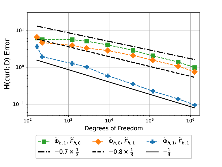
Refer to caption
Figure 1: Error convergence in the 𝑯⁡(𝐜𝐮𝐫𝐥,D)\bm{H}(\operatorname{\mathbf{curl}};\mathrm{D})–norm for the solutions of Problem 3.13 to 𝐄\mathbf{E} –given in (5.4)– depending on the implemented numerical variations of the sesquilinear and antilinear forms, indicated by the legend. The implementation considering Φ~h,e\widetilde{\Phi}_{h,\text{e}} and F~h,e\widetilde{F}_{h,\text{e}} attains a rate of convergence of −13-\frac{1}{3} with respect to the number of degrees of freedom, as predicted by Theorem 3.15. On the other hand, implementations with at least one term not satisfying the conditions of Theorem 3.15 suffer from a degenerated rate between −0.7×13-0.7\times\frac{1}{3} and −0.8×13-0.8\times\frac{1}{3}, but convergence is still observed.

5.2 Convergence estimate for second order finite elements (k=2k=2)

We extend our previous experiment to second order curl-conforming finite elements. Again, we consider μ0=10\mu_{0}=10 and ϵ0=−10\epsilon_{0}=-10, and construct three numerical variations for the sesquilinear form:

Φ~h,0​(𝐔h,𝐕h)\displaystyle\widetilde{\Phi}_{h,0}({\mathbf{U}_{h}},{\mathbf{V}_{h}}) :=∑K∈τhQK1((μ0𝖨)−1𝐜𝐮𝐫𝐥𝐔h⋅𝐜𝐮𝐫𝐥𝐕h¯)+QK1(−ω2(ϵ0𝖨)𝐔h⋅𝐕h¯),\displaystyle:=\sum_{K\in\tau_{h}}Q_{K}^{1}({(\mu_{0}\mathsf{I})}^{-1}\operatorname{\mathbf{curl}}\mathbf{U}_{h}\cdot\operatorname{\mathbf{curl}}\overline{\mathbf{V}_{h}})+Q_{K}^{1}(-\omega^{2}{(\epsilon_{0}\mathsf{I})}\mathbf{U}_{h}\cdot\overline{\mathbf{V}_{h}}),
Φ~h,1​(𝐔h,𝐕h)\displaystyle\widetilde{\Phi}_{h,1}({\mathbf{U}_{h}},{\mathbf{V}_{h}}) :=∑K∈τhQK1((μ0𝖨)−1𝐜𝐮𝐫𝐥𝐔h⋅𝐜𝐮𝐫𝐥𝐕h¯)+QK2(−ω2(ϵ0𝖨)𝐔h⋅𝐕h¯),\displaystyle:=\sum_{K\in\tau_{h}}Q_{K}^{1}({(\mu_{0}\mathsf{I})}^{-1}\operatorname{\mathbf{curl}}\mathbf{U}_{h}\cdot\operatorname{\mathbf{curl}}\overline{\mathbf{V}_{h}})+Q_{K}^{2}(-\omega^{2}{(\epsilon_{0}\mathsf{I})}\mathbf{U}_{h}\cdot\overline{\mathbf{V}_{h}}),
Φ~h,2​(𝐔h,𝐕h)\displaystyle\widetilde{\Phi}_{h,2}({\mathbf{U}_{h}},{\mathbf{V}_{h}}) :=∑K∈τhQK2((μ0𝖨)−1𝐜𝐮𝐫𝐥𝐔h⋅𝐜𝐮𝐫𝐥𝐕h¯)+QK2(−ω2(ϵ0𝖨)𝐔h⋅𝐕h¯),\displaystyle:=\sum_{K\in\tau_{h}}Q_{K}^{2}({(\mu_{0}\mathsf{I})}^{-1}\operatorname{\mathbf{curl}}\mathbf{U}_{h}\cdot\operatorname{\mathbf{curl}}\overline{\mathbf{V}_{h}})+Q_{K}^{2}(-\omega^{2}{(\epsilon_{0}\mathsf{I})}\mathbf{U}_{h}\cdot\overline{\mathbf{V}_{h}}),

where QK˘1Q_{\breve{K}}^{1} is a 2×2×22\times 2\times 2 tensorized Gauss-Legendre quadrature rule –exact on polynomials of degree two on K˘\breve{K}– and QK˘2Q_{\breve{K}}^{2} is a five point Gaussian quadrature rule –exact on polynomials of degree three–. Hence, Φ~h,1\widetilde{\Phi}_{h,1} and Φ~h,2\widetilde{\Phi}_{h,2} satisfy the requirements of Theorem 3.15 with r=1r=1 and 22, respectively. The right-hand side is implemented with a 15 point Gaussian quadrature and is left undisturbed throughout the experiments in this section. Figure 2 displays the convergence of the solution to Problem 3.13 corresponding to the different numerical implementations of the sesquilinear form. 8 meshes with 1,184, 1,688, 7,936, 1,7492, 54,480, 223,652, 674,676 and 2,454,312 degrees of freedom were employed.
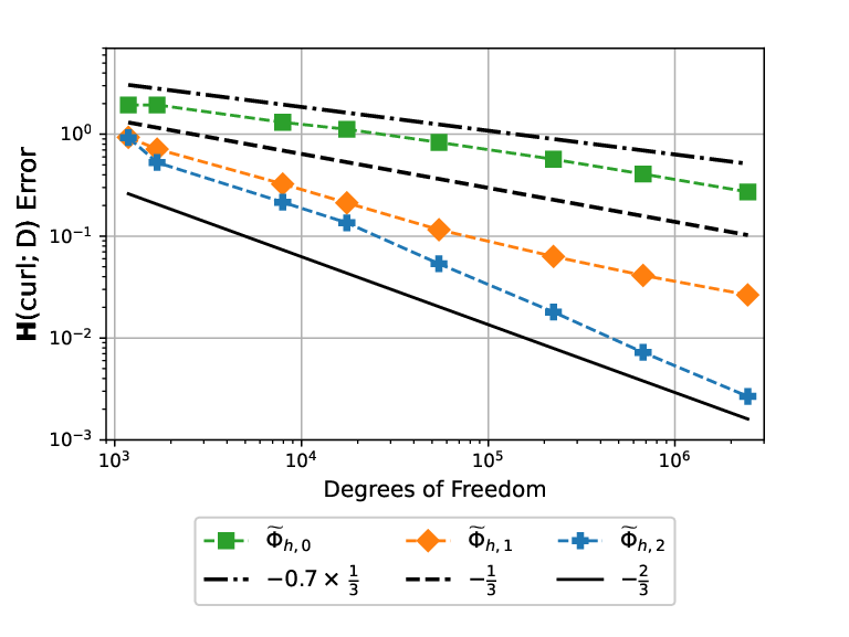
Refer to caption
Figure 2: Error convergence in the 𝑯⁡(𝐜𝐮𝐫𝐥,D)\bm{H}(\operatorname{\mathbf{curl}};\mathrm{D})-norm for the solutions of Problem 3.13 to 𝐄\mathbf{E} –given in (5.4)– depending on the implemented numerical variations of the sesquilinear and antilinear forms, indicated by the legend. The implementation considering Φ~h,2\widetilde{\Phi}_{h,2} and Φ~h,1\widetilde{\Phi}_{h,1} attain their predicted rates of convergence of −23-\frac{2}{3} and −13-\frac{1}{3}, respectively. The implementation considering Φ~h,0\widetilde{\Phi}_{h,0} suffers from a degenerated rate close to −0.7×13-0.7\times\frac{1}{3}, though convergence is still observed.
Remark 5.1.

GETDP does not include an implementation of the second order curl-conforming finite elements defined in Section 3.1. However, an implementation of the second order Webb basis functions [18, 29, 30] is available. Since they are contained in ℙ2​(K˘)\mathbb{P}_{2}(\breve{K}), the consistency estimates in Theorems 3.19 and 3.20 remain valid, so our numerical examples are still meaningful when using this alternative basis.

5.3 Effect of quadrature precision on preasymptotic convergence

We investigate the effect that quadrature precision has on ℓ∈ℕ\ell\in{\mathbb{N}} in Theorem 3.15, i.e., the duration of the preasymptotic regime before convergence is observed at the predicted rate. We consider μ0=10\mu_{0}=10 (as before) and ϵ0=−10−9​sin⁡(m​π​x3)\epsilon_{0}=-10-9\sin(m\pi x_{3}) for two cases m=10m=10 and 2020. The solution to Problem 2.3 is still given by (5.4). We construct our numerical variations for the sesquilinear form as follows

Φ~h,n​(𝐔h,𝐕h)\displaystyle\widetilde{\Phi}_{h,n}({\mathbf{U}_{h}},{\mathbf{V}_{h}}) :=∑K∈τhQK1((μ0𝖨)−1𝐜𝐮𝐫𝐥𝐔h⋅𝐜𝐮𝐫𝐥𝐕h¯)+QK,n2(−ω2(ϵ0𝖨)𝐔h⋅𝐕h¯),\displaystyle:=\sum_{K\in\tau_{h}}Q_{K}^{1}({(\mu_{0}\mathsf{I})}^{-1}\operatorname{\mathbf{curl}}\mathbf{U}_{h}\cdot\operatorname{\mathbf{curl}}\overline{\mathbf{V}_{h}})+Q_{K,n}^{2}(-\omega^{2}{(\epsilon_{0}\mathsf{I})}\mathbf{U}_{h}\cdot\overline{\mathbf{V}_{h}}),

where QK˘1Q_{\breve{K}}^{1} is as before and QK˘,n2Q_{\breve{K},n}^{2} is a Gaussian quadrature over K˘\breve{K} with n=1n=1, 44 and 1515 points. The right-hand side is implemented with a 29 point Gaussian quadrature. Figure 3 displays the convergence of the solution of Problem 3.13 depending on the number of quadrature points used in the implementation of the sesquilinear form. The employed meshes were as in Section 5.1.

Refer to caption
(a) ϵ0=−10−9​sin⁡(10​π​x3)\epsilon_{0}=-10-9\sin(10\pi x_{3})
Refer to caption
(b) ϵ0=−10−9​sin⁡(20​π​x3)\epsilon_{0}=-10-9\sin(20\pi x_{3})
Figure 3: Error convergence in the 𝑯⁡(𝐜𝐮𝐫𝐥,D)\bm{H}(\operatorname{\mathbf{curl}};\mathrm{D})-norm for solutions of Problem 3.13 to 𝐄\mathbf{E} –given in (5.4)– for the two cases of ϵ0\epsilon_{0} and depending on the implemented numerical variations of the sesquilinear form. In both cases, we observe a marked preasymptotic regime when only one quadrature point is implemented, where no convergence is observed before reaching ≈104\approx 10^{4} degrees of freedom and the mesh is able to resolve the oscillatory term in ϵ0\epsilon_{0}. Improving the quadrature rule to 4 points quickly corrects this issue on the case in Figure 3a, though a preasymptotic regime is still observed on the case displayed in Figure 3b, which is improved on by a further increase in precision to 15 quadrature points.

6 Concluding Remarks

Our two main results (Theorems 3.15 and 4.13) yield sufficient conditions to ensure convergence rates for the errors induced by quadrature rules used when solving Maxwell Equations via the FE method with inhomogeneous coefficients and on meshes with curved elements (tetrahedrons). Interestingly, Theorem 3.15 confirm the presumptions of P. Monk in the penultimate paragraph of Section 8.3 in [23], where it is stated that quadrature rules exact on polynomials of degree 2​k−12k-1 are expected to yield convergence rates of order hkh^{k}.

Unlike our result in Section 3, Theorem 4.13 analyses only the quadrature effect in implementation and does not present convergence estimates for the fully discrete solution to the real solution. The result does, however, set aside the issue of numerical integration, so that only the variational crime of the approximation of the real domain is left to be analysed. Notice as well, that choosing 𝔎=1\mathfrak{K}=1 in Section 4 yields the same conditions for the quadrature rules in our two main results, which is of course to be expected.

Numerical examples in Section 5 not only confirm our results, but also display the necessity of the conditions of Theorems 3.15 and 4.13, since implementations that do not satisfy said conditions attain lower convergence rates than implementations that do.

Lastly, though we consider the smoothness of our parameters ϵ\epsilon, μ\mu and 𝐉\mathbf{J} to be global—belonging to some Sobolev space on the whole domain—one could quite easily accommodate our results to consider parameters with piecewise smoothness on a finite set of sub-domains of D\mathrm{D}, by requesting that the two dimensional surfaces across which they fail to posses the required degree of smoothness, does not cross any element of the mesh. In other words, that each of the sub-domains is meshed so that the parameters are smooth on all elements of the mesh. An analogous consideration holds if the domain D\mathrm{D} fails to posses a certain degree of smoothness at a finite number of points on its boundary.

References

  • [1] Assyr Abdulle and Gilles Vilmart. A priori error estimates for finite element methods with numerical quadrature for nonmonotone nonlinear elliptic problems. Numerische Mathematik, 121(3):397–431, 2012.
  • [2] R. Aylwin, C. Jerez-Hanckes, C. Schwab, and J. Zech. Domain uncertainty quantification in computational electromagnetics. Technical Report 2019-04, Seminar for Applied Mathematics, ETH Zürich, Switzerland, 2019.
  • [3] Uday Banerjee. A note on the effect of numerical quadrature in finite element eigenvalue approximation. Numerische Mathematik, 61(1):145–152, 1992.
  • [4] Uday Banerjee and John E Osborn. Estimation of the effect of numerical integration in finite element eigenvalue approximation. Numerische Mathematik, 56(8):735–762, 1989.
  • [5] Uday Banerjee and Manil Suri. The effect of numerical quadrature in the p-version of the finite element method. Mathematics of computation, 59(199):1–20, 1992.
  • [6] Pulin K Bhattacharyya and Neela Nataraj. On the combined effect of boundary approximation and numerical integration on mixed finite element solution of 4th order elliptic problems with variable coefficients. ESAIM: Mathematical Modelling and Numerical Analysis, 33(4):807–836, 1999.
  • [7] A. Buffa, M. Costabel, and D. Sheen. On traces for 𝐇⁡(𝐜𝐮𝐫𝐥,Ω){\bf H}({\bf curl},\Omega) in Lipschitz domains. J. Math. Anal. Appl., 276(2):845–867, 2002.
  • [8] Annalisa Buffa and Ralf Hiptmair. Galerkin boundary element methods for electromagnetic scattering. In Topics in computational wave propagation, volume 31 of Lect. Notes Comput. Sci. Eng., pages 83–124. Springer, Berlin, 2003.
  • [9] Annalisa Buffa, Ralf Hiptmair, Tobias von Petersdorff, and Christoph Schwab. Boundary element methods for Maxwell transmission problems in Lipschitz domains. Numer. Math., 95(3):459–485, 2003.
  • [10] Philippe G Ciarlet. Basic error estimates for elliptic problems. 1991.
  • [11] Philippe G Ciarlet and P-A Raviart. The combined effect of curved boundaries and numerical integration in isoparametric finite element methods. In The mathematical foundations of the finite element method with applications to partial differential equations, pages 409–474. Elsevier, 1972.
  • [12] Phillipe G. Ciarlet. The finite element method for elliptic problems. Society for Industrial and Applied Mathematics, 2002.
  • [13] Daniele A Di Pietro and Jérôme Droniou. A third strang lemma and an aubin–nitsche trick for schemes in fully discrete formulation. Calcolo, 55(3):40, 2018.
  • [14] P. Dular and C. Geuzaine. GetDP reference manual: the documentation for GetDP, a general environment for the treatment of discrete problems. http://getdp.info.
  • [15] Alexandre Ern and Jean-Luc Guermond. Theory and practice of finite elements, volume 159. Springer Science & Business Media, 2004.
  • [16] Alexandre Ern and Jean-Luc Guermond. Finite element quasi-interpolation and best approximation. Mathematical Modelling and Numerical Analysis, 51(4):1367–1385, 2017.
  • [17] Alexandre Ern and Jean-Luc Guermond. Analysis of the edge finite element approximation of the maxwell equations with low regularity solutions. Computers & Mathematics with Applications, 75(3):918–932, 2018.
  • [18] Christophe Geuzaine, B Meys, Patrick Dular, and Willy Legros. Convergence of high order curl-conforming finite elements [for em field calculations]. IEEE transactions on magnetics, 35(3):1442–1445, 1999.
  • [19] Christophe Geuzaine and Jean-François Remacle. Gmsh: A 3-d finite element mesh generator with built-in pre-and post-processing facilities. International journal for numerical methods in engineering, 79(11):1309–1331, 2009.
  • [20] Erwin Hernández and Rodolfo Rodríguez. Finite element approximation of spectral problems with neumann boundary conditions on curved domains. Mathematics of computation, 72(243):1099–1115, 2003.
  • [21] Carlos Jerez-Hanckes, Christoph Schwab, and Jakob Zech. Electromagnetic wave scattering by random surfaces: Shape holomorphy. Mathematical Models and Methods in Applied Sciences, 27(12):2229–2259, 2017.
  • [22] Mo Lenoir. Optimal isoparametric finite elements and error estimates for domains involving curved boundaries. SIAM Journal on Numerical Analysis, 23(3):562–580, 1986.
  • [23] Peter Monk. Finite element methods for Maxwell’s equations. Oxford University Press, 2003.
  • [24] Peter Monk. Finite element methods for Maxwell’s equations. Numerical Mathematics and Scientific Computation. Oxford University Press, New York, 2003.
  • [25] Stefan A. Sauter and Christoph Schwab. Boundary element methods, volume 39 of Springer Series in Computational Mathematics. Springer-Verlag, Berlin, 2011. Translated and expanded from the 2004 German original.
  • [26] Olaf Steinbach. Numerical Approximation Methods for Elliptic Boundary Value Problems. Springer Science & Business Media, 2007.
  • [27] Luc Tartar. An introduction to Sobolev spaces and interpolation spaces, volume 3. Springer Science & Business Media, 2007.
  • [28] Michèle Vanmaele and Alexander Ženíšek. The combined effect of numerical integration and approximation of the boundary in the finite element method for eigenvalue problems. Numerische Mathematik, 71(2):253–273, 1995.
  • [29] Jon P Webb. Hierarchal vector basis functions of arbitrary order for triangular and tetrahedral finite elements. IEEE Transactions on antennas and propagation, 47(8):1244–1253, 1999.
  • [30] JP Webb and B Forgahani. Hierarchal scalar and vector tetrahedra. IEEE Transactions on Magnetics, 29(2):1495–1498, 1993.