marginparsep has been altered.
topmargin has been altered.
marginparwidth has been altered.
marginparpush has been altered.
The page layout violates the ICML style.
Please do not change the page layout, or include packages like geometry, savetrees, or fullpage, which change it for you.
We’re not able to reliably undo arbitrary changes to the style. Please remove the offending package(s), or layout-changing commands and try again.
IOS: Inter-Operator Scheduler for CNN Acceleration
Yaoyao Ding* 1 2 Ligeng Zhu 3 Zhihao Jia 4 Gennady Pekhimenko 1 2 Song Han 3
Proceedings of the MLSys Conference, San Jose, CA, USA, 2021. Copyright 2021 by the author(s).
Abstract
To accelerate CNN inference, existing deep learning frameworks focus on optimizing intra-operator parallelization. However, a single operator can no longer fully utilize the available parallelism given the rapid advances in high-performance hardware, resulting in a large gap between the peak performance and the real performance. This performance gap is more severe under smaller batch sizes. In this work, we extensively study the parallelism between operators and propose Inter-Operator Scheduler (IOS) to automatically schedule multiple operators’ parallel execution through a novel dynamic programming algorithm. IOS consistently outperforms state-of-the-art libraries (e.g., TensorRT) by to on modern CNN benchmarks. The code to reproduce each experiment is available at: https://github.com/mit-han-lab/inter-operator-scheduler.
1 Introduction
Convolutional neural networks (CNNs) have achieved state-of-the-art performance across many tasks, including computer vision Krizhevsky et al. 2012; He et al. 2016, machine translation Sutskever et al. 2014; Devlin et al. 2018, and game playing Mnih et al. 2013; Silver et al. 2016. The success comes at the cost of growing computational requirements. The high demand for computation makes efficient inference more critical in real deployment Han et al. 2015; Chen et al. 2018; Jia et al. 2019a.
A common practice to improve inference efficiency is parallelization. Deep learning frameworks such as Tensorflow Abadi et al. 2016 and Pytorch Paszke et al. 2017 exploit intra-operator parallelism, which parallelizes arithmetic operations within a single CNN operator (e.g., convolution).
However, due to the rapid advances in high-performance hardware, intra-operator parallelism is no longer sufficient to obtain efficient resource utilization. As shown in Figure 1, the peak FP32 performance of a GPU has increased from 5.8 TFLOPs/s in 2013 to 15.7 TFLOPs/s in 2018 (shown in red). NVIDIA Tesla A100 even reaches a peak FP32 performance of 19.5 TFLOPs/s.
Meanwhile, there is a recent trend in CNN design to replace a single branch of convolutions with multiple branches of convolutions, which is advantageous due to increased model capacity under a fixed computation budget Szegedy et al. 2016; Zoph et al. 2018; Xie et al. 2019. As a result, the number of convolutions grows while the computation FLOPs in each convolution becomes smaller. For example, the average floating-point operations (FLOPs) per convolution has decreased from 2330 MFLOPs/kernel in VGG to 82 MFLOPs/kernel in NASNet. This exacerbates the device’s under-utilization problem.

To address this problem, recent work explores inter-operator parallelism by executing multiple CNN operators in parallel guided by different heuristics Tang et al. 2018; Jia et al. 2019b; Ma et al. 2020. For example, MetaFlow Jia et al. 2019b fuses multiple operators matching a specific pattern into a larger operator to increase operator granularity. Tang et al. Tang et al. 2018 proposes a greedy strategy that directly executes all available CNN operators on CPU to maximize resource utilization. These approaches apply different heuristics to optimize local parallelization across a few CNN operators; however, such techniques do not lead to a globally optimal schedule for the entire CNN architecture. For example, given an input CNN (Figure 2 (1)), a greedy schedule (Figure 2 (2)) would perform convolutions [a], [c], and [d] in parallel, and run convolution [b] in a subsequent stage upon the completion of the previous stage.
This greedy schedule is sub-optimal for two reasons. First, a greedy schedule eagerly puts more operators in the early stages (as soon as they are available for execution) and fewer operators in subsequent stages, resulting in low utilization in later stages. Second, executing too many operators on the device concurrently may lead to resource contention problem that hurts the performance. For example, as shown in Figure 2, the greedy schedule (2) suffers from resource contention problem in the first stage and low-utilization problem in the second stage, comparing to our proposed schedule (3).
Obtaining an optimized schedule to parallelize a CNN model is a challenging task. On the one hand, the number of schedules grows exponentially with the number of operators, making it infeasible to evaluate all possible schedules exhaustively. For example, a network with operators can have number of feasible schedules. On the other hand, an optimal schedule also depends on hardware specifications and inference settings (e.g., batch size). A high-end GPU (e.g., Tesla V100) can efficiently execute a schedule with many operators in parallel, while a low-end GPU (e.g., Tesla K80) might suffer from resource contention using the same schedule. A large batch size naturally offers more intra-operator parallelism, while a small batch size has a stronger need for inter-operator parallelization. Therefore, given a diverse set of CNN architectures, hardware, and inference settings, it is hard to devise an efficient schedule manually for all scenarios.
To address this challenge, we propose IOS, an inter-operator scheduler that accelerates CNN inference by combining intra- and inter-operator parallelism. We observe that different schedules share common sub-schedules; thus, IOS adopts a dynamic programming technique to explore the schedule space and finds a highly optimized schedule under low search cost. We evaluate IOS on modern CNN models, including Inception-V3 Szegedy et al. 2016, RandWire Xie et al. 2019, NasNet-A Zoph et al. 2018, and SqueezeNet Iandola et al. 2016. IOS consistently outperforms the sequential schedule and greedy schedule. IOS achieves to inference speedup compared to existing deep learning libraries (e.g., TensorRT). Furthermore, IOS demonstrates the necessity of customizing the scheduling policy for different hardware and inference configurations. IOS can achieve up to inference speedup by customizing the scheduling recipe compared to itself with no customization.
Our contributions are summarized as follows:
- •
We point out a major bottleneck for efficient CNN inference: existing intra-operator parallelism cannot saturate modern hardware’s high parallelism, especially for recent multi-branch CNN models. Inter-operator parallelism is crucial.
- •
We propose a novel dynamic programming algorithm to find a highly optimized schedule for inter-operator parallelization. This technique is platform-agnostic and can serve as a general technique for popular frameworks such as TensorFlow Abadi et al. 2015 and TVM Chen et al. 2018.
- •
We apply IOS to various hardware and inference settings and show that the different configurations require different schedules. We can automatically customize the scheduling policy for different hardware and inference configurations. The specialized schedules consistently outperform existing deep learning libraries with to measured speedup in inference.
2 Background and Related Work
CNN Design. Several lightweight design primitives have been recently introduced to improve the efficiency of CNNs. Examples include SequeezeNet Iandola et al. 2016, MobileNet Sandler et al. 2018 and ShuffletNet Zhang et al. 2018. However, such design patterns cannot fully utilize the hardware. Hardware under-utilization becomes more severe as accelerators are getting more powerful (shown in Figure 1). On the other hand, multi-branch CNNs become a trend in model architecture design, including both manually designed networks Szegedy et al. 2015; Iandola et al. 2016; Szegedy et al. 2016 and the networks discovered by neural architecture search Cai et al. 2018; Zoph et al. 2018. With a fixed computation budget, multi-branch CNNs use more small convolution primitives, which further amplifies the resource under-utilization problem on modern hardware.
Intra-operator Parallelism. Current deep learning frameworks (e.g., TensorFlow and PyTorch) generally focus on intra-operator parallelism, which executes arithmetic operations within a single operator in parallel (e.g., tiled matrix multiplication). Tensorflow and PyTorch are built upon vendor-provided libraries (e.g., cuDNN), a set of DNN compute primitives heavily optimized by vendor engineers to achieve near-peak machine performance. However, these DNN operators are executed sequentially on a hardware device. The degree of parallelism within an operator is limited; thus, intra-operator parallelism cannot provide sufficient parallelizable computation to feed powerful hardware devices. As a result, the hardware is often under-utilized using these frameworks.
Different from manual performance tuning, Auto-Halide Mullapudi et al. 2016, TVM Chen et al. 2018 and Ansor Zheng et al. 2020 exploit intra-parallelism through automatically learning efficient schedule for individual DNN kernels. This automation saves a large amount of engineering effort and can generate more efficient DNN kernels than the manually designed counterparts. However, still, all these libraries only focus on intra-operator parallelism but do not exploit inter-operator parallelism.
Inter-Operator Scheduling. Recent work has explored inter-operator scheduling. Tang et al. Tang et al. 2018 proposes a greedy heuristic approach, Graphi, that executes all available CNN operators whenever possible to saturate CPU’s computation capability. The greedy strategy does not holistically optimize the computation graph’s performance, hence yields unbalanced and sub-optimal schedules. RammerMa et al. 2020 optimizes the execution of DNN workloads by holistically exploiting parallelism through inter- and intra- operator co-scheduling, enabling a richer scheduling space for executing a DNN model. IOS focuses on the inter-operator scheduling and leaves the intra-operator scheduling to the hardware. NimbleKwon et al. 2020 is a DNN engine that supports parallel execution of DNN operators on GPU and minimizes the scheduling overhead using ahead-of-time (AOT) scheduling. The scheduling algorithm used in Nimble does not consider the latency of each operator, while IOS is a profile-based scheduler.
Graph transformation. MetaFlow Jia et al. 2019b performs functional-preserving graph transformations to optimize DNN architectures. Merging operators with the same input enables more parallelism (a larger operator compared to two small sequential operators) and reduces accesses to GPU memories. TASO Jia et al. 2019a further introduces an automated generation of substitution rules and it explores more mathematically equivalent DNN architectures of the input one comparing to MetaFlow. MetaFlow and TASO consider the whole computation graph and search for highly optimized substitution strategies. However, the inter-oprator parallelism utilized by MetaFlow and TASO is still limited as only the same type of operators can be merged.
To address the large schedule space problem, IOS utilizes dynamic programming to take advantage of the common sub-schedules among different schedules. Also, IOS supports concurrent execution of different types of operators, addressing the limitation of MetaFlow and TASO.
3 Problem Definition
This section defines the schedule in IOS and formulates the problem.
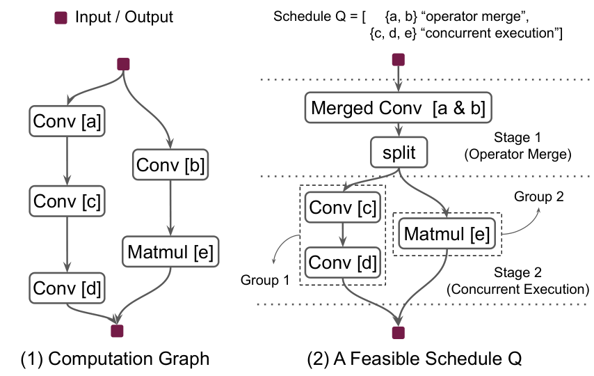
Computation Graph. A CNN is defined by a computation graph , where is the set of operators, and is the edge set representing dependencies. A computation graph is a directed acyclic graph (DAG). Each operator in the graph represents an operator such as convolution and matrix multiplication. Each edge is a tensor that is an output of operator , and an input of operator . Figure 3 (1) shows the computation graph of a simple CNN.
Stage. To take advantage of inter-operator parallelism in a CNN architecture, its computation graph is partitioned into multiple stages. Stages are executed sequentially and the operators in the same stage are executed according to a certain parallelization strategy (see below). Figure 3 (2) shows a possible schedule that partitions the input graph into two stages, where the first stage contains operator a and b, and the second stage contains operator c, d, and e. The parallelization strategy is discussed below.
Parallelization Strategy. Each stage adopts one of the following two parallelization strategies: operator merge and concurrent execution. ISO considers both of them and automatically picks the more efficient one for each stage. The choice depends on operator types, input tensor shapes, and the hardware device to perform CNN computations.
To be eligible for operator merge, the operators’ type must be the same while the hyperparameters can be different. For example, two convolutions with the same stride but different kernel sizes can be merged. The smaller kernel will be padded with zeros to fit the large kernel, so we can stack their kernels together. In Figure 3 (1), if Conv[a] has 128 3x3 kernels while Conv[b] has 256 3x3 kernels, we can stack their kernels together and replace Conv[a] and [b] by a Merged Conv[a&b] with 384 3x3 kernels. Besides increasing parallelism, it also reduces the memory accesses to the input tensor from twice to only once. A split operator is required to partition the merged convolution’s output to recover the original outputs of Conv[a] and Conv[b].
Under concurrent execution, the operators in the stage are partitioned into disjoint groups. More specifically, if two operators are connected by an edge, they are partitioned into the same group. Different groups within the same stage are executed concurrently, while the operators within the same group are executed sequentially. IOS considers simultaneous executions of operators with different types. In the second stage of Figure 3 (2), the three operators are partitioned into two groups. The first group contains operators Conv[c] and Conv[d] while the second group contains operator Matmul[e]. The two groups are executed concurrently while Conv[c] and Conv[d] are executed sequentially in their group.
Schedule. We define a schedule of a computation graph as where is the set of operators in the th stage and is the corresponding parallelization strategy, either “concurrent execution” or “operator merge”. For example, the schedule for Figure 3 (2) is: , . The schedule executes the network from the first stage to the last stage sequentially. may contain only one operator if it is the best choice (e.g., a very large operator that saturates the entire GPU).
Problem Formulation. Let be a cost function defined on a computation graph and schedule . We aim to find a schedule to minimize the cost function for a given computation graph , i.e., . In this work, the cost function is defined as the latency of running following schedule .
4 Methods
This section introduces our Inter-Operator Scheduler (IOS) in three parts. Section 4.1 elaborates the IOS design in details. Section 4.2 analyzes the time complexity of IOS. Finally, Section 4.3 introduces the pruning optimizations to reduce the search time of IOS.
4.1 Inter-Operator Scheduler (IOS)
To find an optimized schedule for a CNN architecture, we first partition its computation graph into and , where all edges between and start from and end in . Such is called an ending of , as illustrated in Figure 4. There can be many endings of . The last stage’s operators in ’s optimal schedule must be an ending of . We can enumerate the ending of and convert the original problem to a sub-problem that finds the optimal schedule for . The whole graph can be scheduled by applying the partition recursively.
Let be the latency of an optimal schedule for . Let be the latency of stage where is the better parallelization strategy for among the two possible ones. We formalize this idea as follows,
where is an ending of , and . Finally, is the latency of an optimal schedule for the entire computation graph . To construct the optimal schedule we found, we record the corresponding that minimizes the latency for each (i.e., ) in .
With this general idea, we implement IOS in three functions InterOperatorScheduler (L3-12), Scheduler (L13-22) and GenerateStage (L23-33), as shown in Algorithm 1. InterOperatorScheduler takes a computation graph as an input and returns the optimal schedule found by IOS. Scheduler is a recursive function implementing the dynamic programming algorithm to find the optimal schedule for a subset of operators in . GenerateStage chooses a better parallelization strategy for given operators .
InterOperatorScheduler (L3-12) is the entry function. It takes a computation graph as an input and returns an optimized schedule . This function calls Scheduler with operators as an argument (L5). After calling Scheduler, the global variable stores the latency of an optimal schedule for , while stores the last stage in the corresponding optimal schedule. Once is obtained, we can construct the schedule found by IOS (L6-11). We start with an empty list as the initial state of our schedule (L6) and let be all the operators in . We inquire about the last stage of by and put it at the head of the current schedule . We repeat this process by letting to get the remaining operators’ schedule in all previous stages (L8-11). indicates that we have discovered an optimized schedule for .
Scheduler (L13-22) is the core part of our algorithm. It implements the dynamic programming algorithm recursivly, taking a subset of as the state. It takes a set of operators as an input and returns the minimal latency for among all schedules. Because Scheduler may be called multiple times with the same argument , for repeated calls, we cache the previous results to avoid redundant computations (L14-15). To find an optimal schedule for , we enumerate its last stage operators and reduce the problem into a sub-problem for (L16-21). We use GenerateStage to choose a better parallelization strategy for and get the latency (L17). is the minimal latency for when taking as the last stage’s operators (L18). We enumerate all possible endings of and record the minimal latency and the corresponding last stage in and , respectively (L19-21).
GenerateStage (L23-33) chooses a better parallelization strategy from “concurrent execution” and “operator merge” for a given stage . It returns the parallelization strategy and the corresponding latency. It directly measures the latencies of both parallelization strategies on the hardware. The “concurrent execution” strategy partitions into multiple disjoint operator groups: . Operators in different groups are executed concurrently while operators in the same group are executed sequentially. For the “operator merge” strategy, if all the operators in can be merged into a single operator (L26), we merge them and measure the latency of the merged operator (L27). Otherwise, we set to infinity to force ourselves to choose the “concurrent execution” strategy.
Figure 5 demonstrates how IOS discovers an optimized strategy for an input graph with three operators a, b, and c. Figure 5 (2) shows the dynamic programming process, the Scheduler in Algorithm 1. For simplicity, we only consider the concurrent execution parallelization strategy. There are six states (the operators to be scheduled, ) in the process. We start with all the operators in the computation graph as state (L5). For each state , Scheduler enumerates the ending of . The latency of contains two parts: latency of as a stage and the latency of . While the result of is measured on the device directly (), the optimal latency of is obtained via solving the sub-problem recursively. to shows the computation path. Note that IOS memorizes the results for each calculated state to avoid redundant computations. Thus, step visits state , and IOS gets its latency directly (L15) because it has been previously visited by step . Scheduler stores the latency () and last stage () in its optimal schedule. We can construct the best schedule for the whole computation graph using , as shown in Figure 5 (3). An optimal schedule found by IOS is shown in (4). Both stages take “concurrent execution” as the parallelization strategy.
4.2 Time Complexity of IOS
In this subsection, we analyze the time complexity of IOS. We take set operations (L18, L24) and latency measurement operations (L25, L27) as atom operations to make the analysis clear. To analyze the time complexity of IOS, we count the number of executions of L17-21, since they dominate the whole algorithm’s execution. This number equals the number of edges (i.e., transitions) in Figure 5 (2). Furthermore, it is equivalent to count the number of pairs , where is a state and is an ending of . Here we define the width of a directed acyclic graph and provide the time complexity of Algorithm 1.
Definition 1 (Width of a DAG).
We call the width of a directed acyclic graph if we can find at most operators in such that there is no path connecting any two of them.
Theorem (Time Complexity of IOS).
The time complexity of Inter-Operator Scheduler (IOS) is , which can be relaxed to , where is the number of operators in the computation graph and is its width.
In fact, there are computation graphs that can reach this bound, so we can not improve it without other restrictions on the schedule space. Proof can be found in Appendix A.
| Model | # | #Schedules | |||
|---|---|---|---|---|---|
| Inception V3 | |||||
| Randwire | |||||
| NasNet | |||||
| SqueezeNet |
Modern convolution neural networks usually construct the network by stacking multiple blocks, making it possible to optimize each block separately. In this case, and refers to the number of operators within a block and the block width, rather than the full network. We list the information of the largest block for each network benchmark in Table 1.
The total number of feasible schedules is exponential to the number of operators (e.g., up to for Randwire Xie et al. 2019). Such a huge number makes it prohibitive to manually design or enumerate the schedules. However, by reusing the results of common sub-schedules in the schedule finding process, IOS finds the optimal schedule within hours for each network with no pruning strategy used. The time complexity of IOS is only exponential to the width of the computation graph, which is usually very small and acceptable (e.g., in all benchmarked networks).
4.3 Reduce the Search Time by Schedule Pruning
It is difficult for a dynamic programming algorithm to stop early, because it gets the best result at the very end. To reduce the search time, IOS introduces schedule pruning to reduce the exploration space by restricting the max number of groups and the max number of operators within a group. We define the pruning strategy as a boolean function of and . We only enumerate the ending of that satisfies the pruning strategy , that is, (L16 of Algorithm 1). The pruning strategy consists of two parameters and : if and only if ending has at most groups and each group has at most operators.
After applying the pruning strategy , the time complexity is reduced from to . Of course, there is a trade-off between the search cost and the quality of the discovered schedule. We evaluate this trade-off in Section 7.1.
5 Implementation Setup
IOS is a framework-agnostic algorithm and can be implemented in popular frameworks. We implement the dynamic programming scheduling algorithm in Python and the execution engine in C++. The latency of a stage is directly measured in the execution engine to guide the scheduling. The execution engine is based on vendor-provided library cuDNN Chetlur et al. 2014 and supports operators’ parallel execution. To concurrently execute multiple groups of operators, IOS puts different groups into different CUDA streams. Kernels in different CUDA streams will be executed in parallel if there are enough computation resources. Throughout the experiments, we use cuDNN 7.6.5, cuda 10.2, NVIDIA driver 450.51.05, and adopt TensorRT 7.0.0.11 and TVM 0.7 as baseline libraries.
| Networks | #Blocks | #Operators | Operator Type |
|---|---|---|---|
| Inception V3 | Conv-Relu | ||
| Randwire | Relu-SepConv | ||
| NasNet | Relu-SepConv | ||
| SqueezeNet | Conv-Relu |
We benchmark four modern CNNs in the experiment: Inception V3 Szegedy et al. 2016, RandWire Xie et al. 2019, NasNet-A Zoph et al. 2018 and SqueezeNet Iandola et al. 2016. Table 2 shows the number of blocks, the number of operators, and the main operator type for each network. IOS supports the user-defined schedule unit. In this experiment, we take the operator type shown in the table, besides other operators such as Concat, as the basic schedule unit. Some models (e.g., ResNet He et al. 2016) might have limited inter-operator parallelization opportunities. For example, for ResNet-50 and ResNet-34, we can only achieve 2% to 5% speedup by paralleling the downsample convolutions. We do not consider it as our benchmarked model in the rest of the evaluation.
We conduct each experiment times and report the average performance. We adopt the schedule pruning strategy with and and conduct each experiment on NVIDIA Tesla V100 unless otherwise stated. Please refer to Appendix B for the experiments on other device. The IOS optimization cost for Inception V3 and SqueezeNet is less than minute and the IOS optimization cost for Randwire and NasNet is within minutes.
6 Experiments
6.1 Comparison of Different Schedules
We first compare the inference performance among different schedules with batch size one. We compare five schedules: sequential schedule, greedy schedule, IOS-Merge schedule, IOS-Parallel schedule, and IOS-Both schedule. The sequential schedule executes the operator one-by-one according to certain topological ordering. The greedy schedule puts all the operators that can be executed currently in one stage, and repeats this process until all operators have been scheduled. IOS-Merge, IOS-Parallel, and IOS-Both schedules use the proposed approach to find the schedule but take different parallelization strategies. IOS-Merge only takes the “operator merge” strategy. IOS-Parallel only takes the “concurrent execution” strategy. IOS-Both considers both parallelization strategies. All schedules are executed on IOS execute engine for a fair comparison.
Figure 7 shows that IOS-Both outperforms all the other four schedules. The greedy schedule gets good results on RandWire and NasNet. However, it degrades the performance of SqueezeNet because of the overhead of synchronization. Because we can not merge “Relu-SepConv” operators in RandWire and NasNet, IOS-Merge gets the same schedule as Sequential, and IOS-Both gets the same schedule as IOS-Parallel. IOS-Both considers two parallelization strategies and outperforms all the other four schedules. In later experiments, “IOS” refers to “IOS-Both” by default.
6.2 Comparison of cuDNN-based Frameworks
For popular frameworks, there are two ways to exploit the intra-operator parallelism. Frameworks such as Tensorflow Abadi et al. 2015, TASO Jia et al. 2019a, and TensorRT NVIDIA use the vendor-provided library cuDNN. Frameworks such as TVM Chen et al. 2018 and Ansor Zheng et al. 2020 search the tensor program schedule for each kernel. TVM also supports to call external libraries such as cuDNN to implement some kernels (e.g., convolution). In this subsection, we compare the performance of cuDNN-based frameworks with batch size one. Larger batch size is studied in the ablation study section.
There are five baselines: Tensorflow, Tensorflow-XLA, TASO, TVM-cuDNN, and TensorRT. Tensorflow-XLA is the tensorflow framework with XLA optimization turning on. TVM-cuDNN is the TVM framework that compiles a convolution neural network with cuDNN library, which would use the convolution kernel provided by cuDNN to execute convolutions. All other operators such as addition and concatenation would use their own kernels. For fair comparison, we only compare cuDNN-based libraries here. The comparison between TVM-AutoTune and IOS can be found in the ablation study section. Figure 7 shows that IOS consistently outperforms all five baseline frameworks on four benchmark CNNs. IOS can achieve to speedup comparing to the state of the art library TASO, TVM-cuDNN, and TensorRT.
6.3 More Active Warps Improve Utilization
Model operators are mapped to GPU kernels to execute. A kernel invokes a collection of threads that are grouped into multiple thread blocks.11 1 We adopt the terminology used by NVIDIA. Thread blocks are distributed to stream multiprocessors (SMs). Each thread block on a SM is further partitioned into multiple warps. A warp, as a basic execution unit, contains a fixed number of threads (e.g., 32 for NVIDIA GPU) to execute in a Single Instruction Multiple Thread (SIMT) fashion.
A warp is considered active from the time it is scheduled on an SM until it completes the last instruction. SM can hide the warps stall caused by memory accesses through fast context switching: at every cycle, each warp scheduler will pick an eligible warp and issue instructions. If no eligible warp is available for a warp scheduler, the computation resources are underutilized. Increasing the number of active warps is an effective approach to increase the likelihood of having eligible warps to execute at each cycle. Thus, it is crucial to increase the number of active warps. Figure 8 shows the number of active warps on the whole GPU throughout the repeated execution of both the IOS and the Sequential schedule, sampled using NVIDIA’s CUPTI profiling toolset every 2.1 ms. IOS schedule achieves more active warps on average compared to the Sequential schedule. This explains the reason for IOS overall performance speedup.
7 Ablation Study
7.1 Schedule Pruning Reduces Search Time
To explore the trade-off between optimized latency and optimization cost (i.e. search time), we experiment Inception V3 and NasNet with pruning strategy parameters and . As shown in Figure 9, when and get smaller, the optimization cost decreases at the cost of larger network latency. This is because smaller and restrict the schedules that IOS explores, thus reduce the optimization cost and increase schedule latency. By setting and , IOS still achieves and speedup for Inception V3 and NasNet, comparing to sequential schedule. Meanwhile, the optimization cost for each network is within seconds and minutes, respectively.
7.2 Specialized Scheduling is Beneficial
![[Uncaptioned image]](2011.01302v2/experiments_specialization_tables.png)
Different workloads (e.g. network with different batch sizes) have different computation features; thus it is necessary to specialize the schedule for different workloads. We optimize Inception V3 with batch size 1, 32 and 128. Then we execute the network with these schedules on batch size 1, 32 and 128 separately. In Table 3 (1), the numbers in a row represents the latency executed with the same batch size but using schedules optimized for different batch sizes. The specialized schedule for each batch size achieved the best result. To explore the specialization for devices, we also optimize the network on both NVIDIA Tesla K80 and V100 with batch size one. Table 3 (2) shows that the specialized schedule for each device also achieved better results.

IOS discovers different schedules for different batch sizes. For example, Figure 10 shows the schedule of the last block of Inception V3 optimized for batch size 1 and 32, respectively. There are two stages in the schedule (1), which is optimized for batch size 1 while there are four stages in the schedule (2), which is optimized for batch size 32. The schedule (1) is 28% faster than the schedule (2) on batch size 1, while the schedule (2) is 8% faster than (1) on batch size 32. There are two differences between them. The first one is that convolution f and g in the schedule (2) are merged into a single convolution. This is because activation (the output tensor of an operator) is the memory bottleneck at large batch size. It is more crucial to reduce memory access, even at the cost of larger computation cost. Merging can reduce the memory access, because the merged kernel only access the output of convolution c once, instead of twice in the schedule (1). However, because the kernel size of f and g are 3x1 and 1x3, respectively, their kernel size would be expanded to 3x3 by padding zeros, which increases the amount of computation. Another difference between the schedule (1) and (2) is that the schedule (2) has more stages than the schedule (1). We found a similar phenomenon for large batch sizes because of resource contention. When multiple operators are executed on the device, there is a conflict over access to the shared resources such as the last-level cache, making the concurrent execution degrades the performance. This gets more severe for larger batch sizes because the demand for shared resources gets larger.
7.3 Consistent Improvement for Different Batch Sizes

In real-world applications, we need to handle different batch sizes for inference. For example, for real-time applications on edge devices, we usually use a batch size of one to reduce latency. In contrast, in cloud settings, the larger batch size is preferred to increase throughput. Changing the workload requires different inter-operator parallelization schedules. We optimize Inception V3 with the batch sizes of 1, 16, 32, 64, 128, and compare the throughput. Figure 11 shows that the throughput increases with the batch size. When the batch size is larger than 128, the performance saturates, and the throughput does not increase significantly anymore. The throughput of IOS outperforms all the baselines consistently on all batch sizes. Even though a larger batch size provides more data parallelism, we can still utilize inter-operator parallelism to further improve the throughput.
7.4 Intra- and Inter-Operator Parallelism
TVM exploits the intra-operator parallelism by searching the schedule for each kernel on a specific device. IOS focuses on inter-operator parallelism and leaves the exploitation of intra-operator parallelism to cuDNN library. Although intra- and inter-operator parallelism is orthogonal and can be combined, we compare TVM and IOS here to give some insight into each parallelism’s benefit. As shown in Figure 12, TVM takes GPU hours while IOS only takes GPU hours to optimize the four networks. IOS outperforms TVM on Inception V3 and SqueezeNet. This is because only utilizing intra-parallelism can not provide enough parallelism for the powerful computing device. Meanwhile, TVM outperforms IOS on Randwire and NasNet, because TVM finds more efficient kernels for separable convolutions, which occupy the majority of operators in Randwire and NasNet. We believe the combination of TVM and IOS would boost the performance further and leave this for future work.
8 Conclusion
With the increasing computational capacity, the sequential execution of CNNs no longer provides sufficient parallelization opportunities to fully utilize all the computation resources. We propose IOS that combines intra- and inter-operator parallelism and adapt dynamic programming to find an efficient schedule that better utilizes the hardware. Experiments show that IOS can improve the GPU utilization and speedup modern CNN inference from to compared to the state-of-the-art libraries (e.g., TensorRT).
Acknowledgements
We want to thank Xiaodan (Serina) Tan for NVIDIA GPU-related issues and constructive discussion. This project was supported by the Canada Foundation for Innovation JELF grant, NSERC Discovery grant, AWS Machine Learning Research Award, Facebook Faculty Research Award, MIT-IBM Watson AI Lab, MIT Data Science and AI Lab (DSAIL), NVIDIA, and NSF CAREER Award #1943349.
References
- Abadi et al. (2015) Abadi, M., Agarwal, A., Barham, P., Brevdo, E., Chen, Z., Citro, C., Corrado, G. S., Davis, A., Dean, J., Devin, M., Ghemawat, S., Goodfellow, I., Harp, A., Irving, G., Isard, M., Jia, Y., Jozefowicz, R., Kaiser, L., Kudlur, M., Levenberg, J., Mané, D., Monga, R., Moore, S., Murray, D., Olah, C., Schuster, M., Shlens, J., Steiner, B., Sutskever, I., Talwar, K., Tucker, P., Vanhoucke, V., Vasudevan, V., Viégas, F., Vinyals, O., Warden, P., Wattenberg, M., Wicke, M., Yu, Y., and Zheng, X. TensorFlow: Large-scale machine learning on heterogeneous systems, 2015. URL http://tensorflow.org/. Software available from tensorflow.org.
- Abadi et al. (2016) Abadi, M., Barham, P., Chen, J., Chen, Z., Davis, A., Dean, J., Devin, M., Ghemawat, S., Irving, G., Isard, M., et al. Tensorflow: A system for large-scale machine learning. In 12th USENIX Symposium on Operating Systems Design and Implementation (OSDI 16), pp. 265–283, 2016.
- Cai et al. (2018) Cai, H., Yang, J., Zhang, W., Han, S., and Yu, Y. Path-level network transformation for efficient architecture search. In ICML, 2018.
- Chen et al. (2018) Chen, T., Moreau, T., Jiang, Z., Zheng, L., Yan, E., Shen, H., Cowan, M., Wang, L., Hu, Y., Ceze, L., et al. TVM: An automated end-to-end optimizing compiler for deep learning. In 13th USENIX Symposium on Operating Systems Design and Implementation (OSDI 18), pp. 578–594, 2018.
- Chetlur et al. (2014) Chetlur, S., Woolley, C., Vandermersch, P., Cohen, J., Tran, J., Catanzaro, B., and Shelhamer, E. cudnn: Efficient primitives for deep learning. arXiv preprint arXiv:1410.0759, 2014.
- Devlin et al. (2018) Devlin, J., Chang, M., Lee, K., and Toutanova, K. BERT: pre-training of deep bidirectional transformers for language understanding. CoRR, abs/1810.04805, 2018. URL http://arxiv.org/abs/1810.04805.
- Dilworth (1950) Dilworth, R. P. A decomposition theorem for partially ordered sets. Annals of Mathematics, 51(1):161–166, 1950. ISSN 0003486X. URL http://www.jstor.org/stable/1969503.
- Han et al. (2015) Han, S., Mao, H., and Dally, W. J. Deep compression: Compressing deep neural networks with pruning, trained quantization and huffman coding. arXiv preprint arXiv:1510.00149, 2015.
- He et al. (2016) He, K., Zhang, X., Ren, S., and Sun, J. Deep residual learning for image recognition. In Proceedings of the IEEE conference on computer vision and pattern recognition, pp. 770–778, 2016.
- Iandola et al. (2016) Iandola, F. N., Han, S., Moskewicz, M. W., Ashraf, K., Dally, W. J., and Keutzer, K. Squeezenet: Alexnet-level accuracy with 50x fewer parameters and 0.5 mb model size. arXiv preprint arXiv:1602.07360, 2016.
- Jia et al. (2019a) Jia, Z., Padon, O., Thomas, J., Warszawski, T., Zaharia, M., and Aiken, A. Taso: Optimizing deep learning computation with automatic generation of graph substitutions. In Proceedings of the 27th ACM Symposium on Operating Systems Principles, SOSP ’19, pp. 47–62, New York, NY, USA, 2019a. Association for Computing Machinery. ISBN 9781450368735. doi: 10.1145/3341301.3359630. URL https://doi.org/10.1145/3341301.3359630.
- Jia et al. (2019b) Jia, Z., Thomas, J., Warszawski, T., Gao, M., Zaharia, M., and Aiken, A. Optimizing dnn computation with relaxed graph substitutions. In Talwalkar, A., Smith, V., and Zaharia, M. (eds.), Proceedings of Machine Learning and Systems, volume 1, pp. 27–39. 2019b.
- Krizhevsky et al. (2012) Krizhevsky, A., Sutskever, I., and Hinton, G. E. Imagenet classification with deep convolutional neural networks. In Advances in neural information processing systems, pp. 1097–1105, 2012.
- Kwon et al. (2020) Kwon, W., Yu, G.-I., Jeong, E., and Chun, B.-G. Nimble: Lightweight and parallel gpu task scheduling for deep learning. In Larochelle, H., Ranzato, M., Hadsell, R., Balcan, M. F., and Lin, H. (eds.), Advances in Neural Information Processing Systems, volume 33, pp. 8343–8354. Curran Associates, Inc., 2020. URL https://proceedings.neurips.cc/paper/2020/file/5f0ad4db43d8723d18169b2e4817a160-Paper.pdf.
- Ma et al. (2020) Ma, L., Xie, Z., Yang, Z., Xue, J., Miao, Y., Cui, W., Hu, W., Yang, F., Zhang, L., and Zhou, L. Rammer: Enabling holistic deep learning compiler optimizations with rtasks. In 14th USENIX Symposium on Operating Systems Design and Implementation (OSDI 20), pp. 881–897. USENIX Association, November 2020. ISBN 978-1-939133-19-9. URL https://www.usenix.org/conference/osdi20/presentation/ma.
- Mnih et al. (2013) Mnih, V., Kavukcuoglu, K., Silver, D., Graves, A., Antonoglou, I., Wierstra, D., and Riedmiller, M. Playing atari with deep reinforcement learning. arXiv preprint arXiv:1312.5602, 2013.
- Mullapudi et al. (2016) Mullapudi, R. T., Adams, A., Sharlet, D., Ragan-Kelley, J., and Fatahalian, K. Automatically scheduling halide image processing pipelines. ACM Transactions on Graphics (TOG), 35(4):1–11, 2016.
- (18) NVIDIA. Nvidia tensorrt: Programmable inference accelerator. URL https://developer.nvidia.com/tensorrt.
- Paszke et al. (2017) Paszke, A., Gross, S., Chintala, S., Chanan, G., Yang, E., DeVito, Z., Lin, Z., Desmaison, A., Antiga, L., and Lerer, A. Automatic differentiation in pytorch. In NIPS-W, 2017.
- Sandler et al. (2018) Sandler, M., Howard, A., Zhu, M., Zhmoginov, A., and Chen, L.-C. Mobilenetv2: Inverted residuals and linear bottlenecks. In Proceedings of the IEEE Conference on Computer Vision and Pattern Recognition, pp. 4510–4520, 2018.
- Silver et al. (2016) Silver, D., Huang, A., Maddison, C. J., Guez, A., Sifre, L., Van Den Driessche, G., Schrittwieser, J., Antonoglou, I., Panneershelvam, V., Lanctot, M., et al. Mastering the game of go with deep neural networks and tree search. nature, 529(7587):484, 2016.
- Sutskever et al. (2014) Sutskever, I., Vinyals, O., and Le, Q. V. Sequence to sequence learning with neural networks. In Advances in neural information processing systems, pp. 3104–3112, 2014.
- Szegedy et al. (2015) Szegedy, C., Liu, W., Jia, Y., Sermanet, P., Reed, S., Anguelov, D., Erhan, D., Vanhoucke, V., and Rabinovich, A. Going deeper with convolutions. In Proceedings of the IEEE conference on computer vision and pattern recognition, pp. 1–9, 2015.
- Szegedy et al. (2016) Szegedy, C., Vanhoucke, V., Ioffe, S., Shlens, J., and Wojna, Z. Rethinking the inception architecture for computer vision. In Proceedings of the IEEE conference on computer vision and pattern recognition, pp. 2818–2826, 2016.
- Tang et al. (2018) Tang, L., Wang, Y., Willke, T. L., and Li, K. Scheduling computation graphs of deep learning models on manycore cpus. arXiv preprint arXiv:1807.09667, 2018.
- Xie et al. (2019) Xie, S., Kirillov, A., Girshick, R., and He, K. Exploring randomly wired neural networks for image recognition. arXiv preprint arXiv:1904.01569, 2019.
- Zhang et al. (2018) Zhang, X., Zhou, X., Lin, M., and Sun, J. Shufflenet: An extremely efficient convolutional neural network for mobile devices. In Proceedings of the IEEE Conference on Computer Vision and Pattern Recognition, pp. 6848–6856, 2018.
- Zheng et al. (2020) Zheng, L., Jia, C., Sun, M., Wu, Z., Yu, C. H., Haj-Ali, A., Wang, Y., Yang, J., Zhuo, D., Sen, K., Gonzalez, J. E., and Stoica, I. Ansor: Generating high-performance tensor programs for deep learning. In 14th USENIX Symposium on Operating Systems Design and Implementation (OSDI 20), Banff, Alberta, November 2020. USENIX Association. URL https://www.usenix.org/conference/osdi20/presentation/zheng.
- Zoph et al. (2018) Zoph, B., Vasudevan, V., Shlens, J., and Le, Q. V. Learning transferable architectures for scalable image recognition. In Proceedings of the IEEE conference on computer vision and pattern recognition, pp. 8697–8710, 2018.
Appendix A Proof of Time Complexity
In this section of appendix, we prove the time complexity bound given in Section 4.2. In Section A.1, we give some preliminary definitions and theorems used in our proof. In Section A.2, we prove the time complexity of inter-operator scheduler (IOS).
A.1 Preliminary Definitions and Theorems
In this subsection, we give the definition of chain and anti-chain, Dilworth’s theorem Dilworth 1950, and a corollary, which is used in our proof later.
Definition 2 (Chain and antichain).
A chain is a subset of a partially ordered set such that any two distinct elements in the subset are comparable. An antichain is a subset such that any two distinct elements in the subset are incomparable.
Definition 3 (Chain decomposition of partial order set).
A chain decomposition of a partial order set is a partition of the elements of the ordered set into disjoint chains.
Theorem (Dilworth’s Theorem).
In any finite partially ordered set, the largest antichain has the same size as the smallest chain decomposition.
We apply the Dilworth’s theorem to a directed acyclic graph and can get the following corollary.
Corollary 1.
Let be a directed acyclic graph and be the width of . We can decompose into sets such that any two vertices in the same set can be connected by a path in .
Proof.
Let be the partial order derived from by transitive closure. Then that two elements in are comparable in is equivalent to that there is a path between them in . Thus, the width of equals the size of largest antichain of . We apply the Dilworth’s Theorem to and can get a decomposition of into chains in : . Because is a chain in , any two elements in are comparable, which means there is a path bridge them in . ∎
A.2 Time Complexity of Inter-Operator Scheduler
In this subsection, we will prove the time complexity of IOS stated in Section 4.2. Then we will show that the upper bound can be reached by some computation graph.
Lemma 1.
If ends and ends , then also ends ( ends means that is an ending of ).
Proof.
We prove it by contradiction. If does not end , there must exist such that and . Then we have or . If , we can get the contradiction that is not an ending of because . If , we can also get the contradiction that is not an ending of because . ∎
Lemma 2.
Let be a possible argument of Scheduler, we have ends .
Proof.
Lemma 3.
Let be a subset of and any two operators in are bridged by a path. Let be the size of . Then
Proof.
Because any two operators in is bridged by a path in , operators in are ordered sequentially. Because ends , there are only possible sets of because must be a prefix in the sequential ordered operators, including empty set. is a suffix of , including empty set. Then there are possible pairs of . ∎
Theorem.
The time complexity of inter-operator scheduler is , which can be relaxed to , where is the number of operators in the computation graph and is its width.
Proof.
We only need to count the number of pairs of that can reach L17 of Algorithm 1 because L17-21 dominates the execution time of the scheduler, where is a subset of that is taken as the argument of Scheduler and is an ending of . By Lemma 2, ends . By Corollary 1, we can decompose into disjoint partitions and any two operators in the same partition can be bridged by a path in . We can build a one-to-one mapping that maps pair to -dimension tuple based on the partition. Then we only need to count the number of valid tuples to get the number of valid pairs. By Lemma 3, the possible number of pairs is . Then an upper bound of the tuples is . It is an upper bound but not the exact number because currently we only consider the dependency inside each partition and ignored the dependency between different partitions. So the upper bound of the number of pairs of is . It can be relaxed to because and it is maximized when are equal. For simplicity, it can be further relaxed to . ∎
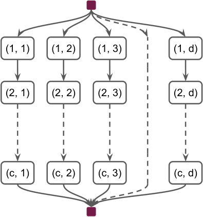
The computation graph shown in Figure 13 is an example to demonstrate that the time complexity of can be reached.
In this example, there are independent paths and each path has operators. Because the paths are independent with each other and there is no edge between two different paths, we can get the upper bound by the analysis in above time complexity proof.
Appendix B Speedup on NVIDIA RTX 2080Ti
In addition to results on NVIDIA Tesla V100 (Volta architecture), we also conduct experiments on NVIDIA RTX 2080Ti (Turing architecture) to show that our optimization is generally effective across different GPU architectures. We use the same models and baselines for comparisons as in Section 6.1 and Section 6.2.
Figure 14 shows that IOS with two parallelization strategies (i.e., IOS-Both) outperforms all other schedules. In particular, IOS-Both achieves to speedup comparing to the sequential schedule. Figrue 15 shows that IOS outperforms all other cuDNN-based frameworks22 2 TASO runs out of GPU memory on NVIDIA 2080Ti for RandWire and NasNet. on Inception V3, RandWire, and NasNet. IOS achieves comparable performance with TASO and TensorRT on SquuezeNet. These results align with the results on V100.
Appendix C Block-wise Speedup
To explore the speedup for different blocks, we compare the performance of each block of Inception-V3 Szegedy et al. 2016 between sequential and IOS schedule (Figure 16). IOS consistently runs faster than the sequential schedule. The speedup for the individual block is up to 2.3, and the end-to-end speedup is 1.6. More speedup is achieved for back blocks because the width gets larger and more inter-parallelism is possible.