Success-or-Draw: A Strategy Allowing Repeat-Until-Success in Quantum Computation

Introduction – Quantum algorithms are an inevitable element for exploiting the potential of quantum computation nielsenchuang; wilde; watrous. In many quantum algorithms, a unitary operation characterizing the problem and its related quantum operations, such as its inverse operation, are used as subroutines. Quantum supermaps describe such relationships between quantum operations, and are used for analyzing higher-order transformations between quantum operations comb1; comb2; comb3. In spite of their concrete formalism, many “useful” supermaps, such as cloning unitary operations unitary_cloning, inverting unitary operations unitary_inversion1; unitary_inversion2; refocusing; storage_retrieval; one_shot_entropy, controlling unitary operations controllization, unitary learning unitary_learning; storage_retrieval, are not physically implementable in an exact and deterministic manner. In order to perform such supermaps, two types of relaxation are usually considered: the approximate transformation and the probabilistic transformation. In addition to these relaxations, adding certain resources is also considered, especially by allowing multiple calls of an input quantum operation. In the quantum circuit implementation, multiple calls are achievable by using the corresponding quantum circuit multiple times. With the assumption of multiple calls, the strategy to approximate supermaps has an advantage because it is always possible to perform process tomography process_tomography to obtain a classical description of the input quantum operation, calculate the output quantum operation of the supermap, and implement the output quantum operation according to the classical description. On the other hand, it is not known in general whether we can perform a supermap probabilistically but exactly, even if an arbitrary but finite number of calls are allowed.

Quantum process tomography process_tomography allows a universal and approximate implementation of quantum supermaps, but the figure of merit, usually the average fidelity $F$, is expected to scale as $1-1/poly(N)$ given $N$ calls of the input operation. The probabilistic strategy, on the other hand, can achieve a success probability converges to one exponentially, if it is possible to perform independent trials such as in a repeat-until-success protocol. That is, if we can perform a probabilistic supermap with probability $p$ using “a unit of resources” such as one quantum operations, we can perform this probabilistic supermap with probability $1-(1-p)^{N}$ using $N$ units of resources. However, the resources required to perform a supermap are not only the input quantum operations, the input state which the output quantum operation of the supermap is applied on, should also be counted as a resource. In quantum mechanics, transformations usually disturb quantum states wolf; information_disturbance, and the input state of a probabilistic supermap is usually changed regardless of success or failure, that is, the input state is lost after a trial of a supermap. Also, the cloning of a quantum state is forbidden by the no-cloning theorem nocloning. Thus, it is not possible to simply perform independent trials. On the other hand, while allowing multiple copies of an input state may help in certain tasks ncopy, it is difficult to realize in many cases. For such reason, we consider probabilistic supermaps under the following assumption, which is also a well-studied scenario in many previous researches unitary_cloning; unitary_inversion1; unitary_inversion2; refocusing; storage_retrieval; controllization; unitary_learning; storage_retrieval; pbt1; pbt2; unitary_conjugate: multiple calls of an input quantum operation are allowed, and only a single use of an input state is available.

In this paper, we propose a structure of probabilistic supermap called “success-or-draw” structure as Fig. 1a shows. In a usual probabilistic supermap, the input state is lost when it fails because an unknown quantum operation, which is the output quantum operation of the probabilistic supermap on failure, is applied on the input state, such as in the universal programmable quantum processor by port-based teleportation pbt1; pbt2 and the probabilistic store and retrieve of unitary operations storage_retrieval. This fact together with the impossibility to clone the quantum state makes another trial to be not possible. However, while it is not possible to clone the quantum state, it is not known if it is possible to “keep” the quantum state when a probabilistic supermap fails. Thus, we propose a probabilistic supermap which “keeps” the quantum state on failure, or we call it a draw as we are able to perform another trial when it happens as Fig. 1b shows. To summarize, a success-or-draw supermap has the following structure: when it is success, the target quantum operation is obtained; when it is draw, the identity operation is obtained; and the probability of success and draw sum up to one.

Is it always possible to find a success-or-draw supermap for a given task? In Refs. unitary_inversion1; unitary_inversion2, the probabilistic unitary inversion, which is a supermap transforming a unitary operation into its inverse, has been analyzed in the multiple calls scenario, and it is shown that the success-or-draw structure can be achieved by a construction of the quantum circuit. In this paper, we show that the success-or-draw structure can be achieved for a larger class of supermaps by using a certain number of copies of an input quantum operation. Precisely, if there exists a probabilistic supermap transforming a single $d$-dimensional unitary operation into an arbitrary completely positive and trace-preserving (CPTP) map, then it is possible to construct a success-or-draw supermap with $d$ copies of the input unitary operation. In particular, if a supermap is completely CP preserving (CCPP), a condition corresponding to complete positivity (CP) of quantum operations, it is probabilistically implementable comb3. Even if a supermap is not probabilistically implementable, in case that the supermap is linear, its approximated version, e.g., the structural physical approximation spa1; spa2, is probabilistically implementable. Thus, this result applies to all linear supermaps on unitary operations if an approximation is also considered.

This result indicates that if there exists a probabilistic supermap transforming a unitary operation into a CPTP map, then the success probability of this supermap can approach one exponentially by allowing multiple calls of the input unitary operation. Moreover, the corresponding physical realization is given by repetitive trials of a single block of probabilistic supermap as shown in Fig. 1b, and the cost for building the corresponding quantum circuit does not increase with the number of calls.

Success-or-Draw Supermap – We first review the basics of supermaps. A supermap that is using the input quantum operations in a fixed order is known as a quantum comb, and is the one that can be implemented in the usual quantum circuit model. In Refs. comb1; comb2, a formulation of a quantum comb is presented. In order to avoid confusion, we denote quantum operations with a tilde and supermaps with a double tilde. For example, given a unitary operator $U$, we denote the corresponding unitary operation by $\widetilde{\mbox{$\mathcal{U}$}}$. A deterministic comb is described by a CCPP supermap with a set of linear constraints. A probabilistic comb, consists of a success part and a failure part, can be described with two supermaps, say ${\mathchoice{\widetilde{\hbox{$\displaystyle\widetilde{\mbox{$\mathcal{S}$}}$}}}{\widetilde{\hbox{$\textstyle\widetilde{\mbox{$\mathcal{S}$}}$}}}{\widetilde{\hbox{$\scriptstyle\widetilde{\mbox{$\mathcal{S}$}}$}}}{\widetilde{\hbox{$\scriptscriptstyle\widetilde{\mbox{$\mathcal{S}$}}$}}}}$ and ${\mathchoice{\widetilde{\hbox{$\displaystyle\widetilde{\mbox{$\mathcal{F}$}}$}}}{\widetilde{\hbox{$\textstyle\widetilde{\mbox{$\mathcal{F}$}}$}}}{\widetilde{\hbox{$\scriptstyle\widetilde{\mbox{$\mathcal{F}$}}$}}}{\widetilde{\hbox{$\scriptscriptstyle\widetilde{\mbox{$\mathcal{F}$}}$}}}}$ respectively, which sum up to a deterministic comb.

Consider the probabilistic supermap transforming unitary operations $\{\widetilde{\mbox{$\mathcal{U}$}}\}$ into CPTP maps $\{f(\widetilde{\mbox{$\mathcal{U}$}})\}$. In the usual setting of a probabilistic supermap, this problem is formulated by the constraints

For the success-or-draw supermap, the action on failure is also determined, and extra constraints on ${\mathchoice{\widetilde{\hbox{$\displaystyle\widetilde{\mbox{$\mathcal{F}$}}$}}}{\widetilde{\hbox{$\textstyle\widetilde{\mbox{$\mathcal{F}$}}$}}}{\widetilde{\hbox{$\scriptstyle\widetilde{\mbox{$\mathcal{F}$}}$}}}{\widetilde{\hbox{$\scriptscriptstyle\widetilde{\mbox{$\mathcal{F}$}}$}}}}$ are required. For the convenience for the following discussions, we also assume that we have $K$ calls to the input unitary operation $\widetilde{\mbox{$\mathcal{U}$}}$. Since any unitary operation is transformed into the identity operation on failure, the corresponding constraints are given by

where $\widetilde{\mbox{$id$}}$ denotes the identity operation, indicating that the input state does not change on failure. Here we use ${\mathchoice{\widetilde{\hbox{$\displaystyle\widetilde{\mbox{$\mathcal{N}$}}$}}}{\widetilde{\hbox{$\textstyle\widetilde{\mbox{$\mathcal{N}$}}$}}}{\widetilde{\hbox{$\scriptstyle\widetilde{\mbox{$\mathcal{N}$}}$}}}{\widetilde{\hbox{$\scriptscriptstyle\widetilde{\mbox{$\mathcal{N}$}}$}}}}$ instead of ${\mathchoice{\widetilde{\hbox{$\displaystyle\widetilde{\mbox{$\mathcal{F}$}}$}}}{\widetilde{\hbox{$\textstyle\widetilde{\mbox{$\mathcal{F}$}}$}}}{\widetilde{\hbox{$\scriptstyle\widetilde{\mbox{$\mathcal{F}$}}$}}}{\widetilde{\hbox{$\scriptscriptstyle\widetilde{\mbox{$\mathcal{F}$}}$}}}}$ to denote that it corresponds to draw instead of failure, and this condition is also known as the neutralization condition introduced in Ref. controllization.

Main Result – Theorem 1 is the main result on the realizability of success-or-draw supermap. A pictorial interpretation of Theorem 1 is given by Fig. 2.

The proof of Theorem 1 is given in Appendix sm, which includes Ref. ggm_basis. The proof is constructive. We present a construction of the combs ${\mathchoice{\widetilde{\hbox{$\displaystyle\widetilde{\mbox{$\mathcal{S}$}}$}}}{\widetilde{\hbox{$\textstyle\widetilde{\mbox{$\mathcal{S}$}}$}}}{\widetilde{\hbox{$\scriptstyle\widetilde{\mbox{$\mathcal{S}$}}$}}}{\widetilde{\hbox{$\scriptscriptstyle\widetilde{\mbox{$\mathcal{S}$}}$}}}}$ and ${\mathchoice{\widetilde{\hbox{$\displaystyle\widetilde{\mbox{$\mathcal{N}$}}$}}}{\widetilde{\hbox{$\textstyle\widetilde{\mbox{$\mathcal{N}$}}$}}}{\widetilde{\hbox{$\scriptstyle\widetilde{\mbox{$\mathcal{N}$}}$}}}{\widetilde{\hbox{$\scriptscriptstyle\widetilde{\mbox{$\mathcal{N}$}}$}}}}$ from the comb ${\mathchoice{\widetilde{\hbox{$\displaystyle\widetilde{\mbox{$\mathcal{S}$}}$}}}{\widetilde{\hbox{$\textstyle\widetilde{\mbox{$\mathcal{S}$}}$}}}{\widetilde{\hbox{$\scriptstyle\widetilde{\mbox{$\mathcal{S}$}}$}}}{\widetilde{\hbox{$\scriptscriptstyle\widetilde{\mbox{$\mathcal{S}$}}$}}}}_{t}$, more precisely, we show a construction of $S$ and $N$, the Choi operators jamiolkowski; choi; comb1; comb2 of ${\mathchoice{\widetilde{\hbox{$\displaystyle\widetilde{\mbox{$\mathcal{S}$}}$}}}{\widetilde{\hbox{$\textstyle\widetilde{\mbox{$\mathcal{S}$}}$}}}{\widetilde{\hbox{$\scriptstyle\widetilde{\mbox{$\mathcal{S}$}}$}}}{\widetilde{\hbox{$\scriptscriptstyle\widetilde{\mbox{$\mathcal{S}$}}$}}}}$ and ${\mathchoice{\widetilde{\hbox{$\displaystyle\widetilde{\mbox{$\mathcal{N}$}}$}}}{\widetilde{\hbox{$\textstyle\widetilde{\mbox{$\mathcal{N}$}}$}}}{\widetilde{\hbox{$\scriptstyle\widetilde{\mbox{$\mathcal{N}$}}$}}}{\widetilde{\hbox{$\scriptscriptstyle\widetilde{\mbox{$\mathcal{N}$}}$}}}}$, from $S_{t}$, the Choi operator of ${\mathchoice{\widetilde{\hbox{$\displaystyle\widetilde{\mbox{$\mathcal{S}$}}$}}}{\widetilde{\hbox{$\textstyle\widetilde{\mbox{$\mathcal{S}$}}$}}}{\widetilde{\hbox{$\scriptstyle\widetilde{\mbox{$\mathcal{S}$}}$}}}{\widetilde{\hbox{$\scriptscriptstyle\widetilde{\mbox{$\mathcal{S}$}}$}}}}_{t}$. The requirements for the combs are given by Eqs. (4)-(7), which need to be satisfied simultaneously.

While we only require that $S+N$ is a deterministic comb, that is, the input operations are used in a sequential way, the construction shown in the proof (Eq. (S43) of Appendix sm) satisfies an extra condition

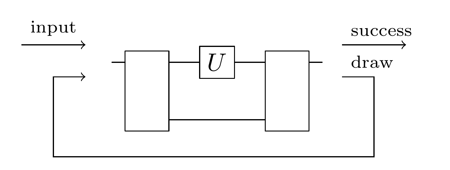
where ${\mathcal{O}}_{0},\ldots,{\mathcal{O}}_{d}$ are the Hilbert spaces as shown in Fig. 2. This condition shows that the comb can be decomposed into two blocks as the quantum circuit shown in Fig. 3: the first block uses only a single unitary operation, while the second block uses the remaining $d-1$ unitary operations in parallel. Such a structure indicates that while the number of calls increases with $d$, the depth of this comb is constant as two. Note that we can assume this structure if we only consider non-zero success probability, and in general, adding this assumption would decrease the success probability.

When the indefinite causal order indefinite1; indefinite2; indefinite3; indefinite_purification is considered, the construction can be replaced by a simpler one by exploiting the symmetry as Remark 2, and a higher success probability can be achieved in general.

Unitary Inversion – In this section, we analyze the probabilistic unitary inversion as a success-or-draw supermap. We only consider the two-dimensional case $d=2$ here. The optimal success probability can be obtained by the following SDP

where $S$ and $N$ denote the Choi operators of the combs corresponding to success and draw, $J_{\Lambda}$ denotes the Choi operator of a quantum operation $\Lambda$, and $\{U_{i}\}$ is a finite set of unitary operators that the corresponding Choi operators form a basis of the linear span of $\mathrm{span}\{J_{U}^{\otimes k}\}$ (see Refs. unitary_inversion1; unitary_inversion2).

For $K=2$, Theorem 1 indicates that the optimal success probability is positive as $p>0$. In fact, a numerical solution to this SDP shows that the optimal success probability is $p=1/3$. This problem is also considered in Ref. unitary_inversion1, where an explicit quantum circuit with the success-or-draw structure was presented, which success probability is $1/4$.

For comparison, we briefly state the protocol presented in Ref. unitary_inversion1. The protocol is similar to the teleportation protocol, which generates the state $\sigma_{x}^{i}\sigma_{z}^{j}|{\psi}\rangle$ before correction, where $|{\psi}\rangle$ is the initial state and $(i,j)=(0,0),(0,1),(1,0),(1,1)$ is the outcome of the Bell measurement. For the two-dimensional unitary inversion protocol presented in Ref. unitary_inversion1, we can obtain $U^{-1}\sigma_{x}^{i}\sigma_{z}^{j}|{\psi}\rangle$ with a single use of $U$ by a small modification to the teleportation or gate teleportation protocol. This protocol successfully achieves unitary inversion when $(i,j)=(0,0)$. When it fails, on the other hand, we can obtain the state $\sigma_{x}^{i}\sigma_{z}^{j}|{\psi}\rangle$ by an extra use of $U$, and the input state $|{\psi}\rangle$ can be recovered by applying $(\sigma_{x}^{i}\sigma_{z}^{j})^{-1}$, which achieves the neutralization supermap.

One difference between the optimal success-or-draw protocol we obtained and the protocol presented in Ref. unitary_inversion1 is that the latter is not only a success-or-draw protocol, but it has another feature: it can be regarded as a success-or-resetting protocol. The latter protocol uses a single copy of a unitary operation to obtain its inverse, and when it fails, it results in a state that is “resettable” to be the input state by another unitary operation. Such a success-or-resetting protocol may have an advantage as we can choose whether to continue the protocol by resetting after we know if it succeeded.

For $K=1$, we also prove that the optimal success probability is $p=0$, which means it is not possible to have a success-or-draw protocol. This result gives an explicit example that a success-or-draw protocol is not available. The proof is given in Appendix sm.

Discussions – We have introduced a new structure for probabilistic supermap which we name success-or-draw structure. A probabilistic supermap with the success-or-draw structure can amplify its success probability by more calls of the input quantum operation in a sequential manner, which scales exponentially to one in the number of calls. A mathematical formulation for the success-or-draw supermap was presented. We considered the case where the input quantum operation is a unitary operation, and we proved that any probabilistic supermap transforming unitary operations into CPTP maps can become a success-or-draw supermap by adding the number of copies of the unitary operation.

We then analyzed the problem of the two-dimensional unitary inversion. When two copies of an input unitary operation are allowed, Theorem 1 guarantees the existence of a non-trivial solution to this problem, and we also obtained the optimal solution numerically using SDP. A success-or-draw protocol for this problem was also presented previously in Ref. unitary_inversion1, and our numerical calculation shows that a higher success probability can be achieved if we only require the success-or-draw structure. We also proved that a success-or-draw protocol does not exist with a single copy of an input unitary operation.

Our result shows an advantage of probabilistic supermap, as it allows a success probability exponentially close to one in the sequential case. The number of calls is also undetermined for a success-or-draw protocol, and an average number of calls may become a suitable measure in practice. We also hope that the success-or-draw structure helps in a simpler physical implementation of supermaps.