Ridge regression with adaptive additive rectangles and other piecewise functional templates

Edoardo Belli Email: edoardo.belli@polimi.it Affiliation: MOX - Modeling and Scientific Computing, Department of Mathematics, Politecnico di Milano, Italy Simone Vantini Email: simone.vantini@polimi.it Affiliation: MOX - Modeling and Scientific Computing, Department of Mathematics, Politecnico di Milano, Italy

Abstract

We propose an $L_{2}$ -based penalization algorithm for functional linear regression models, where the coefficient function is shrunk towards a data-driven shape template $\gamma$ , which is constrained to belong to a class of piecewise functions by restricting its basis expansion. In particular, we focus on the case where $\gamma$ can be expressed as a sum of $q$ rectangles that are adaptively positioned with respect to the regression error. As the problem of finding the optimal knot placement of a piecewise function is nonconvex, the proposed parametrization allows to reduce the number of variables in the global optimization scheme, resulting in a fitting algorithm that alternates between approximating a suitable template and solving a convex ridge-like problem. The predictive power and interpretability of our method is shown on multiple simulations and two real world case studies.

1 Introduction

As the the dimensionality of data sets kept increasing in the last decades, it is no surprise that variable selection in linear models is still a major topic of discussion between statistical and machine learning researchers. The main objective of these methods is to reduce prediction error by decreasing the variance of the predictions, at the expense of an increase in bias, while at the same time allowing for an interpretable model by discarding and/or shrinking the least relevant variables. Arguably the most intuitive approach is best subset selection, where between the $p$ variables, we retain only the subset of size $k<p$ that minimizes the error. Despite that, the combinatorial nature of these techniques is prone to higher variability and computational cost if compared to the shrinkage approach (Hastie et al. 2009), which is usually based on a penalized least squares formulation. The fact that ridge regression (Hoerl and Kennard 1970) uniformly shrinks all the regression coefficients often leads to nonsparse solutions that do not have a clear interpretation, even when the prediction error is low. By penalizing the $\ell_{1}$ norm of the coefficients’ vector, the lasso (Tibshirani 1996) can be seen as a convex relaxation of best subset selection, and is able to produce sparse models often without sacrificing the predictive performance. There is a vast literature that encompasses multiple aspects of these types of methods, including nonconvex penalties like the SCAD (Fan and Li 2001) and MCP (Zhao et al. 2010), refer to Hastie et al. 2015 for an extensive view on sparsity in multivariate linear models.

In the context of functional data analysis (FDA) (Ramsay and Silverman 2005; Ferraty and Vieu 2006), the concept of sparsity has multiple connotations (James 2011) and here we will refer to the sparsity of the regression function $\beta$ , which selects the subsets of the domain where the predictors have no effect on the response. From the theoretical point of view, the scalar on function linear model is ill-posed and there is the need to introduce some form of regularization as an identifiability constraint. The the two main approaches involve either restricting the number of basis functions for the expansion of $\beta$ , like in the case of designer bases and functional principal components (Cai and Hall 2006), or fixing a rich enough basis while applying a suitable penalization on $\beta$ , usually an $L_{2}$ penalty on its $m$ -th derivative to impose smoothness (Cardot et al. 2003; Cardot et al. 2007; Crambes et al. 2009; Yuan and Cai 2010) as well as sparsity inducing ones like the group SCAD (Matsui and Konishi 2011). Hybrid approaches have also been proposed, where the number of basis functions is adaptively chosen while an additional penalty is included (Marx and Eilers 1999; Lee and Park 2012), or sparsity is imposed on the $m$ -th derivatives of $\beta$ (James et al. 2009). In this work we will adopt the penalization approach and in particular we express $\beta$ as a finite expansion on a simple grid basis with $p$ dense and equispaced knots on the input data:

\beta(t)=\sum_{j=1}^{p}\beta_{j}b_{j}(t)\hskip 42.67912ptb_{j}(t)=\begin{cases}1&\hskip 2.84544pt\text{if}\hskip 5.69046pt\frac{j-1}{p}<t\leq\frac{j}{p}\\ 0&\hskip 2.84544pt\text{otherwise}\end{cases}

which is a common choice that allows to use any multivariate method to compute the coefficients $\beta_{j}$ of the expansion and consequently recover $\beta$ . While at glance this may seem a very constrained setting, as the functional covariates could have been sampled on different grids with noise and missing values, a standard practice is to estimate the true functions individually by means of interpolation or smoothing, which are then evaluated on the same dense and equispaced grid to obtain the actual discrete data set. This estimation process is adequate when the raw data has been collected with high resolution techniques, as in chemometrics, environmental or electrical engineering applications. If however the raw data contains few and exceptionally sparse observations over $t$ , as in the case of longitudinal studies, the previous estimation approach fails as there is not enough information to recover the single function individually. A solution to this problem is to use functional principal components with mixed effects (Brumback and Rice 1998; James et al. 2000) or local smoothing (Yao et al. 2005) in order to jointly leverage the information of the full raw data set for the estimation of each functional covariate.

In this work, we are interested in those penalization approaches that beyond pure sparsity, allow to impose some degree of structure to the regression coefficients/function, like joint sparsity and smoothness as in the case of the elastic net (Zou and Hastie 2005) and other $\ell_{1}/\ell_{2}$ combined approaches (Hebiri and van de Geer 2011), imposing an order between the coefficients (Tibshirani and Suo 2016) and especially the fused lasso (Tibshirani et al. 2005), which allows to recover a piecewise constant regression function. Although not in the scope of our investigation, starting from the group lasso (Yuan and Lin 2006), multiple works have dealt with the assumption of a known grouping structure between the covariates, including sparsity and competing variables within the groups (Simon et al. 2013; Breheny 2015; Zhou et al. 2010; Campbell and Allen 2017), overlapping groups (Zhao et al. 2009; Jacob et al. 2009) and supervised clustering-based groups (She 2010). In principle, our method could be used as a preprocessing step to estimate such grouping structure. It is also worth to note that other non penalty-based approaches force $\beta$ to be convex by selecting the maximum between $K$ hyperplanes, where each hyperplane is obtained by fitting a linear model using only a subset of the observations (Magnani and Boyd 2009; Hannah and Dunson 2013).

From a practical standpoint, the type of penalty can be seen as an hyperparameter that has to be selected, either by cross-validation or by domain knowledge, and the availability of different options allows researchers and engineers to tackle a multitude of $p>>N$ scenarios. However, current methods are not flawless, as in the case of the lasso where the number of non-zero coefficients that can be recovered is at most $N$ , which can be a limiting factor and may exclude important variables, especially in the presence of highly collinear functional data, where the irrepresentable condition is often violated and selection consistency is not guaranteed (Meinshausen and Bühlmann 2006; Zhao and Yu 2006). Therefore, the design of new penalties is still an open problem, and our proposal aims to add further modeling flexibility to the user, by allowing a parsimonious and yet adaptive formulation of the shape $\gamma$ that we want to impose on $\beta$ , by expressing $\gamma$ as a finite sum of a few user-defined piecewise basis functions like a rectangular pulse. In particular, our method is based on the nonzero centered $L_{2}$ penalty (Swindel 1976; Price et al. 2015; van Wieringen 2019; Bilgrau et al. 2020) and uses a global optimization scheme in order to adaptively find a suitable and possibly sparse shape template that will be the target of the shrinkage, with the objective to reduce bias.

The article is organized as follows: in Section 2 we explain our method together with the optimization details, Section 3 contains multiple simulation studies and two real world applications, with concluding remarks in Section 4.

2 Adaptive additive piecewise functional templates

Let $\mathcal{D}=\{(x_{i},y_{i})\}_{i=1}^{N}$ be the training set with random i.i.d. functions $x_{i}\in L^{2}(I)$ and responses $y_{i}\in\mathbb{R}$ , we study the scalar on function regression model:

y_{i}=\beta_{0}+\int_{I}x_{i}(t)\beta(t)dt+\epsilon_{i}

(1)

where $\beta_{0}\in\mathbb{R}$ is the intercept and $\epsilon_{i}\sim\mathcal{N}(0,\sigma^{2})$ random i.i.d. errors. Without loss of generality, we will assume that the regressors have been standardized and that $I=[-1,1]$ . For a given template function $\gamma:[-1,1]\rightarrow\mathbb{R}$ , we estimate the linear model by solving the following problem:

\underset{\mathchoice{\raisebox{-1.67998pt}{\resizebox{1265808}{393216}{\hbox{\raisebox{1.3611pt}{$\displaystyle\beta_{0},\beta$}}}}}{\raisebox{-1.67998pt}{\resizebox{1265808}{393216}{\hbox{\raisebox{1.3611pt}{$\textstyle\beta_{0},\beta$}}}}}{\raisebox{-1.68pt}{\resizebox{1215662}{393216}{\hbox{\raisebox{0.95277pt}{$\scriptstyle\beta_{0},\beta$}}}}}{\raisebox{-2.59201pt}{\resizebox{1382797}{393216}{\hbox{\raisebox{1.05pt}{$\scriptscriptstyle\beta_{0},\beta$}}}}}}{\mathchoice{\raisebox{0.0pt}{\resizebox{1267876}{458752}{\hbox{\raisebox{0.0pt}{$\displaystyle min$}}}}}{\raisebox{0.0pt}{\resizebox{1267876}{458752}{\hbox{\raisebox{0.0pt}{$\textstyle min$}}}}}{\raisebox{0.0pt}{\resizebox{1472617}{458752}{\hbox{\raisebox{0.0pt}{$\scriptstyle min$}}}}}{\raisebox{0.0pt}{\resizebox{1818849}{458752}{\hbox{\raisebox{0.0pt}{$\scriptscriptstyle min$}}}}}}\>\>\>\sum_{i=1}^{N}\left[y_{i}-\beta_{0}-\int_{I}x_{i}(t)\beta(t)dt\right]^{2}+\lambda\int_{I}\big[\beta(t)-\gamma(t)\big]^{2}dt

(2)

which is an $L_{2}$ -penalized least squares with $\beta$ shrunk towards $\gamma$ instead of zero, and $\lambda>0$ the hyperparameter that controls the amount of shrinkage. While the template function $\gamma$ can be directly provided by the user, in this work we propose an adaptive global optimization approach for the choice of $\gamma$ , which we restrict to belong to the following class of functions $\Gamma$ :

\Gamma=\left\{\gamma\!:[-1,1]\rightarrow\mathbb{R}\;\Bigg|\;\gamma(t)=\sum_{j=1}^{q}A_{j}g_{j}\left(t,t_{0j},T_{j}\right)\right\}

		$\displaystyle q\in\mathbb{N}^{+}$
		$\displaystyle A_{j}\in\mathbb{R}$
		$\displaystyle t_{0j}\in[-1,1]$
		$\displaystyle T_{j}\in(0,2]$

where each of the $g_{j}\left(t_{0j},T_{j}\right):[-1,1]\rightarrow\mathbb{R}$ can be an arbitrary but known piecewise function such that the knots that define the intervals depend on $t_{0j}$ and $T_{j}$ . This means that $\gamma$ can be expressed as a finite expansion with piecewise basis functions that are chosen adaptively. In fact, $g_{j}$ could be any user-defined function parametrized by $t_{0j}$ and $T_{j}$ , but we will focus on the case where $g_{j}=g_{i}$ for $j\neq i$ , dropping the subscript for ease of notation, with $g$ being a rectangular function:

g\left(t,t_{0},T\right)=\begin{cases}1&\>\text{if}\>\left|\frac{t-t_{0}}{T}\right|\leq\frac{1}{2}\\ 0&\>\text{otherwise}\end{cases}\hskip 28.45274pt\includegraphics[valign,width,trim,clip]{figs/rect_example.pdf}

The choice of the rectangular shape allows correlated parts of the domain to be equally included in the model and has a straightforward interpretation. While this template based approach could appear to be too rigid, expressing $\gamma$ as a sum of $q$ adaptively positioned rectangles seems to provide the flexibility needed to avoid sacrificing prediction error, maintaining at the same time a sound regularization effect. Moreover, once the expansion of $\gamma$ is optimized, the impact on $\beta$ is further controlled by selecting $\lambda$ by cross-validation, as the regression function is not expanded with respect to the same restricted basis, but instead uses the rich enough grid basis. This is an important aspect of our method, as optimizing $\gamma$ is equivalent to the problem of selecting the optimal number and position of the knots in free-knot splines, which is known to be nonconvex (de Boor 1973) even for univariate functions. Multiple heuristics have been proposed to tackle this problem, including nonlinear optimization (Jupp 1978; Lindstrom 1999), using the lasso to determine the knots (Osborne et al. 1998) or fixing a large number of equidistant knots while penalizing the squared finite differences of the coefficients of adjacent B-splines (Eilers and Marx 1996). Many successful approaches are built on algorithmic stepwise addition/removal of knots (Friedman and Silverman 1989; Breiman 1991; Friedman 1991), with locally adaptive splines (Mammen and van de Geer 1997) that are based on total variation penalization on derivatives and enjoy optimal rates of convergence in bounded variation function classes, also for linear splines that saturate (are constant) outside the data range (Boyd et al. 2018). The stepwise addition approach has also been used in FDA for the estimation of the mean and the covariance function of a set of curves (Gervini 2006). In the case of trend filtering (Kim et al. 2009) the positions of the knots are adaptively chosen by specifying a suitable discrete difference operator of some order and solving a generalized lasso problem. In fact, for first order differences/constant trend, this reduces to the fused lasso with univariate inputs and pure fusion penalty. Moreover, the trend filtering estimate in the constant or piecewise-linear case is shown to be equal to the adaptive spline estimate (Tibshirani 2014). Our approach is instead based on derivative-free optimization, which has already been used to select the knot vector for B-splines (Pittman 2002), for density-based approximation of univariate piecewise linear functions (Pittman and Murthy 2000) and in supervised dimensionality reduction for classification problems with a functional regressor (Tian and James 2013), where the basis for the expansion of the input functions is chosen between a set of simple shapes, through a stochastic search algorithmic procedure that exploits the class membership. Altough in a different context, this last work is similar in spirit to ours, as it leverages both interpretable shapes and derivative-free optimization to select them. In particular, both approaches avoid working at the full knot level and allow to define any number of black-box basis shapes, but we provide a different parametrization for the shapes and a different algorithm for the optimization. As previously mentioned, while the types of basis $g_{j}$ could be considered as hyperparameters, we will focus on rectangular shapes only. The number of basis functions $q$ is fixed before the optimization but is instead selected by cross-validation, usually between $Q=\{1,2,3\}$ to aid interpretability, as higher values of $q$ would lead to a less restricted $\gamma$ , while at the same time increasing the computational cost. This results in a total of $3q$ variables in the global optimization problem, which are $A_{j}$ , $t_{0j}$ and $T_{j}$ for $j$ = $1,\dots,q$ . In fact, we will show that the variables $A_{j}$ that control the heights of the rectangles can be optimized in closed form, further reducing the number of variables to $2q$ , where for the $j$ -th rectangle, $t_{0j}$ controls the horizontal shift with respect to the origin and $T_{j}$ determines the support.

2.1 Fitting algorithm

In order to fit the model, we propose a two step iterative algorithm that is based both on global optimization and $L_{2}$ -penalized least squares. The iterative part of the algorithm aims to mitigate the fact that the heuristic steps could provide inadequate values for $\gamma$ , allowing for some degree of correction.

Given the number of shapes $q$ , which is fixed a priori and chosen with grid search, let $A$ = $\left(A_{1},\dots,A_{q}\right)^{\top}$ , $t_{0}$ = $\left(t_{01},\dots,t_{0q}\right)^{\top}$ and $T$ = $\left(T_{1},\dots,T_{q}\right)^{\top}$ , the first step consists in solving the following problem:

\underset{\mathchoice{\raisebox{-1.70729pt}{\resizebox{2058724}{393216}{\hbox{\raisebox{1.3611pt}{$\displaystyle A,t_{0},T$}}}}}{\raisebox{-1.70729pt}{\resizebox{2058724}{393216}{\hbox{\raisebox{1.3611pt}{$\textstyle A,t_{0},T$}}}}}{\raisebox{-1.7073pt}{\resizebox{1960266}{393216}{\hbox{\raisebox{0.95277pt}{$\scriptstyle A,t_{0},T$}}}}}{\raisebox{-2.63416pt}{\resizebox{2194265}{393216}{\hbox{\raisebox{1.05pt}{$\scriptscriptstyle A,t_{0},T$}}}}}}{\mathchoice{\raisebox{0.0pt}{\resizebox{1267876}{458752}{\hbox{\raisebox{0.0pt}{$\displaystyle min$}}}}}{\raisebox{0.0pt}{\resizebox{1267876}{458752}{\hbox{\raisebox{0.0pt}{$\textstyle min$}}}}}{\raisebox{0.0pt}{\resizebox{1472617}{458752}{\hbox{\raisebox{0.0pt}{$\scriptstyle min$}}}}}{\raisebox{0.0pt}{\resizebox{1818849}{458752}{\hbox{\raisebox{0.0pt}{$\scriptscriptstyle min$}}}}}}\>\>\>\sum_{i=1}^{N}\left[y_{i}-\bar{y}-\int_{I}x_{i}(t)\sum_{j=1}^{q}A_{j}g\left(t,t_{0j},T_{j}\right)dt\right]^{2}

(3)

where $\bar{y}=N^{-1}\sum_{i=1}^{N}y_{i}$ and $N$ is the size of the training set. This is a least squares formulation in which the regressor function is hard-constrained to belong to $\Gamma$ . The objective function of Problem 3 is nonconvex but marginally convex in $A$ , therefore we approximate the solution with a heuristic approach that will be described in the next subsection. The resulting shape template $\gamma^{init}$ is now recovered from $\left(A^{*},t_{0}^{*},T^{*}\right)$ and Problem 2 is solved with $\gamma=\gamma^{init}$ and a given $\lambda$ , obtaining $\tilde{\beta}$ . With the intention of improving on the current solution $\tilde{\beta}$ , which depends on the initial approximation of $\gamma$ , we can iterate the process by reshaping $\gamma$ towards $\tilde{\beta}$ , through the following problem:

\underset{\mathchoice{\raisebox{-1.70729pt}{\resizebox{2058724}{393216}{\hbox{\raisebox{1.3611pt}{$\displaystyle A,t_{0},T$}}}}}{\raisebox{-1.70729pt}{\resizebox{2058724}{393216}{\hbox{\raisebox{1.3611pt}{$\textstyle A,t_{0},T$}}}}}{\raisebox{-1.7073pt}{\resizebox{1960266}{393216}{\hbox{\raisebox{0.95277pt}{$\scriptstyle A,t_{0},T$}}}}}{\raisebox{-2.63416pt}{\resizebox{2194265}{393216}{\hbox{\raisebox{1.05pt}{$\scriptscriptstyle A,t_{0},T$}}}}}}{\mathchoice{\raisebox{0.0pt}{\resizebox{1267876}{458752}{\hbox{\raisebox{0.0pt}{$\displaystyle min$}}}}}{\raisebox{0.0pt}{\resizebox{1267876}{458752}{\hbox{\raisebox{0.0pt}{$\textstyle min$}}}}}{\raisebox{0.0pt}{\resizebox{1472617}{458752}{\hbox{\raisebox{0.0pt}{$\scriptstyle min$}}}}}{\raisebox{0.0pt}{\resizebox{1818849}{458752}{\hbox{\raisebox{0.0pt}{$\scriptscriptstyle min$}}}}}}\sum_{i=1}^{N}\left[y_{i}-\bar{y}-\int_{I}x_{i}(t)\sum_{j=1}^{q}A_{j}g\left(t,t_{0j},T_{j}\right)dt\right]^{2}+\lambda\int_{I}\Big[\tilde{\beta}(t)-\sum_{j=1}^{q}A_{j}g\left(t,t_{0j},T_{j}\right)\Big]^{2}dt

(4)

where $\tilde{\beta}$ is fixed from the previous step. As in the case of Problem 3, the objective function of Problem 4 is also nonconvex but marginally convex in $A$ , and the optimization details will also be discussed in the next subsection. Once the new shape template $\gamma$ is recovered, we can solve again Problem 2 (with the same $\lambda$ ) to obtain a refined $\tilde{\beta}$ . These last two steps can be repeated for any number of iterations, with a small reduction of the training loss as the termination condition, and/or a maximum number of iterations. While it is clear that there is no guarantee to find a good shape template, if $\gamma$ is not suitable for the regression task at hand, the chosen $\lambda$ will be small so as to avoid shrinking $\beta$ towards a shape that would result in a poor fit, as $\lambda$ is selected with grid search after the initialization step, regardless of the number of iterations that we run. Beyond visual inspection of $\tilde{\beta}$ , this allows to use the resulting value of $\lambda$ as a further indicator of the reasonableness of the shape $\gamma$ for the current problem. To summarize, let $Q$ be the maximum number of shapes from which $q$ is to be selected and let $M$ be the length of the grid of values from which $\lambda$ is selected, we fit the linear regression model by running Algorithm 1 on the data set $\mathcal{D}$ , obtaining the fitted values $\tilde{\beta}^{*}$ and $\tilde{\beta_{0}}^{*}$ .

Algorithm 1 Ridge Regression with Adaptive Additive Functional Templates

1: for

q=1,\dots,Q

2: Solve Problem 3 with

x_{i}\in\mathcal{D}

3: end for

\rightarrow

\gamma^{init}_{1},\dots,\gamma^{init}_{Q}

5: K-fold split

\mathcal{D}

\mathcal{D}_{k-train}

and

\mathcal{D}_{k-val}

6: for

q=1,\dots,Q

7: for

m=1,\dots,M

8: Solve Problem 2 with

\gamma

\gamma^{init}_{q}

\lambda

\lambda_{m}

x_{i}\in\mathcal{D}_{k-train}

\rightarrow

\tilde{\beta}_{qm}

\tilde{\beta_{0}}_{qm}

10: while Error on

\mathcal{D}_{k-train}

decreases do

11: Solve Problem 4 with

\tilde{\beta}

\tilde{\beta}_{qm}

12:

\rightarrow

\gamma_{qm}

13: Solve Problem 2 with with

\gamma

\gamma_{qm}

\lambda

\lambda_{m}

x_{i}\in\mathcal{D}_{k-train}

14:

\rightarrow

\tilde{\beta}_{qm}

\tilde{\beta_{0}}_{qm}

15: end while

16: Test

\tilde{\beta}_{qm}

\tilde{\beta_{0}}_{qm}

\mathcal{D}_{k-val}

17: end for

18: end for

19:

\rightarrow

q^{*}

m^{*}

20: Refit on the full training set

\mathcal{D}

21: Solve Problem 2 with

\gamma

\gamma^{init}_{q^{*}}

\lambda

\lambda_{m^{*}}

x_{i}\in\mathcal{D}

22:

\rightarrow

\tilde{\beta}^{*}

\tilde{\beta_{0}}^{*}

23: while Error on

\mathcal{D}

decreases do

24: Solve Problem 4 with

\tilde{\beta}

\tilde{\beta}^{*}

25:

\rightarrow

\gamma^{*}

26: Solve Problem 2 with with

\gamma

\gamma^{*}

\lambda

\lambda_{m^{*}}

x_{i}\in\mathcal{D}

27:

\rightarrow

\tilde{\beta}^{*}

\tilde{\beta_{0}}^{*}

28: end while

29: return

\tilde{\beta}^{*}

\tilde{\beta_{0}}^{*}

2.2 Optimization and computational details

Finding the global optimum of a nonconvex function is in general NP-hard and multiple approaches have been proposed to compute approximate solutions in different contexts. When the objective function is of real variables, smooth, and cheap to evaluate, derivative-based methods can leverage gradients to find local minima. A more general approach, which is also suitable for combinatorial problems, is the derivative-free one, where black-box evaluations of the objective function are used in conjunction with different stochastic selection and/or sampling schemes. In practice, the two approaches are often implemented jointly, where derivative-free techniques are used for an initial search of the solution space and identification of prospect points, followed by local gradient-based optimization (Locatelli and Schoen 2016). Another distinction that is often made is the one between single point methods, where a single solution is refined during the iterations, and population-based methods, where the selection schemes rely on a pool of candidate solutions. In this work we propose a hybrid approach based on differential evolution (DE) (Storn and Price 1997) with a closed form solution for a subset of the variables. DE is a derivative-free population-based algorithm that generates new points by perturbation of existing solutions, which is suitable for problems with real variables. In particular, at each iteration three distinct points with indexes $i,j,k$ are randomly selected from the population, and a new candidate is computed by adding to point $k$ the scaled difference between points $i$ and $j$ . There are multiple variants of this base scheme, and for an in depth analysis refer to Price et al. 2005. The choice of DE was motivated by its success in multiple areas, including clustering (Paterlini and Krink 2006) and global plus local search (Locatelli et al. 2014).

Regarding our method, we already mentioned that the objectives in Problem 3 and 4 are nonconvex, as they try to optimize the knot placement of a piecewise function. Restricting $\gamma$ in $\Gamma$ reduces the number of variables to $A_{j}$ , $t_{0j}$ and $T_{j}$ for $j$ = $1,\dots,q$ , instead of directly optimizing the full knot vector, which is often high dimensional. Recall the following simplified definitions of marginal convexity and marginally optimum coordinate:

Definition 2.1 (Marginal convexity).

A function of two variables $J(x,y):\mathbb{R}^{p}\times\mathbb{R}^{q}\rightarrow\mathbb{R}$ is marginally convex in $x\in\mathbb{R}^{p}$ if $\>\forall y\in\mathbb{R}^{q}$ , the function $J_{y}(x):\mathbb{R}^{p}\rightarrow\mathbb{R}$ is convex.

Definition 2.2 (Marginally optimum coordinate).

We say that $\tilde{x}\in\mathbb{R}^{p}$ is marginally optimal with respect to $\tilde{y}\in\mathbb{R}^{q}$ if $\>\forall x\in\mathbb{R}^{p}$ , $J(\tilde{x},\tilde{y})\leq J(x,\tilde{y})$ .

The property of marginal convexity lays the foundation for the alternating minimization principle, which is often used in nonconvex optimization problems where the objective function is marginally convex with respect to the single variables, but not jointly convex with respect to all variables (Jain and Kar 2017). Unfortunately our setting is quite different, as the objective functions of Problem 3 and 4 are not marginally convex in $t_{0}$ and $T$ but only in $A$ . In fact, the variables $A_{j}$ for $j$ = $1,\dots,q$ do not control the position of the knots, but only the height of the $q$ shape templates $g_{j}$ , and in particular both problems are quadratic in $A$ , allowing us to optimize $T$ and $t_{0}$ with DE while recovering the marginally optimal $A$ in closed form, as shown in A.1 and A.2. From the asymptotical standpoint, running Algorithm 1 involves solving Problem 2 and computing the marginally optimal $A$ , which can both be done in $O(p^{3})$ . In practice however, it is arduous to provide a formal analysis, as the total cost is vastly dominated by the global optimization part, which overall depends on the total number of DE iterations. In particular, while the initialization of $\gamma$ is done only $Q$ times, Problem 4 is instead solved multiple times to select the optimal values for $\lambda$ and $q$ . For this reason, we allocate the major part of the DE computational budget to the initalization of $\gamma$ , as the following alternating iterations depend on a suitable initial value. Finally, it is worth to note that all the for loops in Algorithm 1 can be executed in parallel, as the problems are separable with respect to $q$ and $\lambda$ . As for the implementation, our global optimization scheme heavily relies on the Nevergrad library by Facebook Research (Rapin and Teytaud 2018).

3 Applications

In this section we show the performance of our proposed method (AATR as adaptive additive template ridge) in multiple simulation studies and two real world applications. We compare AATR with other functional linear models with known penalties like the lasso, fused lasso, ridge, roughness penalty, elastic net, elastic SCAD, elastic MCP, and we also include the minimum norm least squares solution (mnlstsq) as a reference. Besides AATR and the roughness penalized model, for which we provide our own code, all the other implementations are from scikit-learn (Pedregosa et al. 2011) except for the fused lasso which is available in the CRAN package genlasso (Arnold and Tibshirani 2020) and the elastic SCAD and elastic MCP that are available in the CRAN package ncvreg (Breheny 2020).

3.1 Simulation studies

The objective of the simulations is to show the behaviour of our method in different scenarios, where the true coefficient function $\beta$ is either a mixture of $q$ = $1/2/3$ rectangles or a smooth shape that in principle is not compatible with a rectangle-based penalization, resulting in four different shapes tested. All the simulations share the same base model for the input data, which is a cubic B-spline with 40 inner knots equispaced between $[-2,2]$ , while the spline coefficients are sampled from a multivariate normal for each of the $N$ observations. In particular, we repeat the analysis with two different settings, one with independent spline coefficients, and the other with highly dependent ones, for a total of eight configurations. Once the coefficients are generated and the functional model is determined for the single experiment, the regressors $x_{i}$ are obtained by evaluating the functions in $p$ = $200$ equispaced points in $[-1,1]$ , while the responses $y_{i}$ are computed according to Equation 1 with $\beta_{0}$ = $0$ and $\epsilon_{i}\sim\mathcal{N}(0,1)$ . The sample size is fixed at $N$ = $100$ for all the experiments. Figures 1, 2 and 3 portray the input curves and the fitted coefficient functions for the configurations with $q$ = $1$ , while Figures 4, 5 and 6 show the case $q$ = $2$ , Figures 7, 8 and 9 show the case $q$ = $3$ and finally Figures 10, 11 and 12 illustrate the smooth scenario. The results for all the simulations are presented together in Table 1, which reports the mean regression error on the test set obtained by 3-fold cross-validation of the $N$ samples. The hyperparameters are selected with grid search by 3-fold cross-validation on the current split. It is worth noting that for a given configuration, the method with the lowest error is not always the one that is closer to recovering the correct shape, and overall the fused lasso and AATR are the ones that are able to better approximate the true pattern. While the $L_{1}$ norm allows the fused lasso to find nonsmooth coefficient functions, with the fusion penalty in particular that imposes the piecewise constant behaviour, AATR achieves similar results by smooth $L_{2}$ shrinkage towards a nonsmooth shape. This is clear by looking at Figure 3 for instance, where AATR recovers a shape that is a rectified version of the one resulting from the roughness penalized model or the ridge, keeping a smooth behaviour in the artifacts outside of the rectangular part, where instead the fused lasso produces the same artifacts, but in a piecewise constant fashion. A similar argument can be held for the case in which the true $\beta$ is smooth and not sparse, where as expected the roughness penalty performs best. Moreover, similarly to the ”elastic” methods that are able to produce both smooth and sparse solutions, AATR will produce sparse solutions only if the shape $\gamma$ itself is sparse. On the downside, the main limitation of AATR is its high reliance on the heuristic approximation of $\gamma$ , for both the initialization and the subsequent iterations. While finding a suitable initial value can drastically reduce the number of alternating iterations, often to a single one as we empirically observed in our experiments, it is also true that the number of variables in the global optimization problem grows (linearly) with the number of basis $q$ , making our approach viable only for small values of $q$ .

Refer to caption — (a) $x_{i}$ - independent

(a) lasso

(b) elastic net

(d) elastic MCP

(e) roughness

(f) ridge

(g) AATR

(h) fused lasso

Figure 2: Independent spline coefficients: fitted coefficient functions

\tilde{\beta}

by penalty type

(a) lasso

(b) elastic net

(d) elastic MCP

(e) roughness

(f) ridge

(g) AATR

(h) fused lasso

Figure 3: Highly dependent spline coefficients: fitted coefficient functions

\tilde{\beta}

by penalty type

(a) lasso

(b) elastic net

(d) elastic MCP

(e) roughness

(f) ridge

(g) AATR

(h) fused lasso

Figure 5: Independent spline coefficients: fitted coefficient functions

\tilde{\beta}

by penalty type

(a) lasso

(b) elastic net

(d) elastic MCP

(e) roughness

(f) ridge

(g) AATR

(h) fused lasso

Figure 6: Highly dependent spline coefficients: fitted coefficient functions

\tilde{\beta}

by penalty type

(a) lasso

(b) elastic net

(d) elastic MCP

(e) roughness

(f) ridge

(g) AATR

(h) fused lasso

Figure 8: Independent spline coefficients: fitted coefficient functions

\tilde{\beta}

by penalty type

(a) lasso

(b) elastic net

(d) elastic MCP

(e) roughness

(f) ridge

(g) AATR

(h) fused lasso

Figure 9: Highly dependent spline coefficients: fitted coefficient functions

\tilde{\beta}

by penalty type

(a) lasso

(b) elastic net

(d) elastic MCP

(e) roughness

(f) ridge

(g) AATR

(h) fused lasso

Figure 11: Independent spline coefficients: fitted coefficient functions

\tilde{\beta}

by penalty type

(a) lasso

(b) elastic net

(d) elastic MCP

(e) roughness

(f) ridge

(g) AATR

(h) fused lasso

Figure 12: Highly dependent spline coefficients: fitted coefficient functions

\tilde{\beta}

by penalty type

Table 1: Regression results for all the simulations: mean-square error

	independent spline coefficients				dependent spline coefficients
	$q$ =1	$q$ =2	$q$ =3	smooth	$q$ =1	$q$ =2	$q$ =3	smooth
mnlstsq	$1.857\,\pm\,.81$	$1.833\,\pm\,.78$	$1.567\,\pm\,.54$	$1.848\,\pm\,.80$	$1.483\,\pm\,.62$	$1.483\,\pm\,.62$	$1.483\,\pm\,.62$	$1.483\,\pm\,.62$
ridge	$1.343\,\pm\,.45$	$1.309\,\pm\,.38$	$1.338\,\pm\,.46$	$1.308\,\pm\,.34$	$1.063\,\pm\,.11$	$1.132\,\pm\,.20$	$1.141\,\pm\,.23$	$1.083\,\pm\,.17$
roughness	$1.235\,\pm\,.35$	$1.399\,\pm\,.21$	$1.335\,\pm\,.27$	$1.183\,\pm\,.33$	$1.036\,\pm\,.03$	$1.145\,\pm\,.14$	$1.115\,\pm\,.16$	$0.948\,\pm\,.01$
lasso	$0.999\,\pm\,.31$	$1.225\,\pm\,.49$	$1.435\,\pm\,.50$	$1.307\,\pm\,.36$	$1.029\,\pm\,.02$	$1.093\,\pm\,.16$	$1.196\,\pm\,.18$	$1.140\,\pm\,.21$
elastic net	$0.999\,\pm\,.31$	$1.222\,\pm\,.49$	$1.327\,\pm\,.48$	$1.244\,\pm\,.30$	$1.028\,\pm\,.02$	$1.087\,\pm\,.15$	$1.119\,\pm\,.11$	$1.070\,\pm\,.14$
elastic SCAD	$1.317\,\pm\,.14$	$2.867\,\pm\,.72$	$4.678\,\pm\,1.4$	$6.598\,\pm\,1.4$	$2.552\,\pm\,.59$	$7.938\,\pm\,.38$	$15.51\,\pm\,3.8$	$5.295\,\pm\,1.1$
elastic MCP	$1.282\,\pm\,.51$	$1.993\,\pm\,.67$	$3.721\,\pm\,1.3$	$3.662\,\pm\,1.2$	$1.923\,\pm\,.43$	$5.957\,\pm\,.42$	$14.27\,\pm\,3.4$	$5.634\,\pm\,1.7$
fused lasso	$0.967\,\pm\,.28$	$1.041\,\pm\,.19$	$1.278\,\pm\,.23$	$1.275\,\pm\,.33$	$1.017\,\pm\,.05$	$0.940\,\pm\,.04$	$1.048\,\pm\,.08$	$1.040\,\pm\,.05$
AATR	$1.019\,\pm\,.24$	$1.052\,\pm\,.29$	$1.253\,\pm\,.28$	$1.344\,\pm\,.43$	$0.975\,\pm\,.05$	$0.960\,\pm\,.08$	$1.012\,\pm\,.01$	$1.011\,\pm\,.06$

3.2 Solar radiation

The first real world application that we present belongs to the renewable energy/smart grid field, and is about predicting the mean daily solar radiation by looking at the daily temperature curves. The full data set is available on kaggle at https://www.kaggle.com/dronio/SolarEnergy and was originally provided by NASA through the Space Apps challenge. As the raw measurements are irregularly sampled during the day, with roughly one measurement every five minutes, we estimate the underlying daily temperature functions by using penalized free-knot cubic splines (Dierckx 1993), which are then evaluated on an equispaced grid of length $p$ = $300$ , while the raw solar radiation measurements are instead averaged over the day. The sample size is $N$ = $39$ days and is obtained after removing some outliers that had constant temperature values over most of the day. The daily temperature profiles are shown with the fitted coefficient functions in Figure 13, where all methods seem to highlight some type of contrast between the temperature during the afternoon and the evening hours. Figure 14 depicts the behaviour of $\beta$ in Problem 2 for increasing values of $\lambda$ , where as expected, higher values of $\lambda$ shrink $\beta$ towards the current $\gamma$ , while Figure 15 instead shows the progression of the different shapes $\gamma$ resulting from Problem 4 with $\lambda$ and $q$ fixed, where the algorithm stops after one iteration, as the initial value obtained from Problem 3 is already the one with the lowest train error. Table 2 reports the mean regression error on the test set obtained by 5-fold cross-validation, with nested grid search by 3-fold cross-validation on the current split for hyperparameter selection.

Figure 15: Solar radiation: initial

\gamma

resulting from Problem 3 and subsequent values obtained by solving Problem 4

Table 2: Solar radiation: regression results, mean-square error

mnlstsq	$3701\,\pm\,1987$
ridge	$1445\,\pm\,625$
roughness	$1521\,\pm\,389$
lasso	$1626\,\pm\,670$
elastic net	$1513\,\pm\,568$
elastic SCAD	$1383\,\pm\,578$
elastic MCP	$1378\,\pm\,567$
fused lasso	$1326\,\pm\,383$
AATR	$958\,\pm\,231$

3.3 London bike sharing

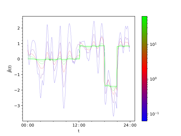
The second real world application is about one of London’s bike sharing systems, and the full dataset is also available on kaggle at https://www.kaggle.com/hmavrodiev/london-bike-sharing-dataset. We focus on predicting the average daily (log) count of bikes by looking at the daily (feels like) temperature curves. The data is measured every hour and therefore each day has at most 24 points. As the sample size of the original dataset is large, we select only the weekend days where all the measurements are available, which results in $N$ = $195$ days. Note that weekend and midweek days typically have very distinct renting patterns and therefore it makes sense to separate the data for this kind of analysis. The underlying temperature functions are estimated by cubic interpolating B-splines, which are then evaluated on the same equispaced grid of length $p$ = $200$ . As in the previous case study, the daily temperature profiles are shown with the scaled coefficient functions in Figure 16, while Figure 17 illustrates the behaviour of $\beta$ in Problem 2 for increasing values of $\lambda$ , and Figure 18 depicts the progression of $\gamma$ with $\lambda$ and $q$ fixed. The results are also obtained by 5-fold cross-validation with the same grid search scheme for hyperparameter selection and are reported in Table 3. It is worth to note that the two best performing methods, AATR and the roughness penalized model, are the ones that also show a coherent behaviour in their respective coefficient functions, despite the obvious difference in smoothness.

Figure 18: London bike sharing: initial

\gamma

resulting from Problem 3 and subsequent values obtained by solving Problem 4

Table 3: London bike sharing: regression results, mean-square error

mnlstsq	$.0931\,\pm\,.0397$
ridge	$.0506\,\pm\,.0213$
roughness	$.0488\,\pm\,.0194$
lasso	$.0523\,\pm\,.0236$
elastic net	$.0514\,\pm\,.0218$
elastic SCAD	$.0543\,\pm\,.0222$
elastic MCP	$.0529\,\pm\,.0228$
fused lasso	$.0496\,\pm\,.0207$
AATR	$.0486\,\pm\,.0187$

4 Conclusions

Shrinkage methods are widely used in high dimensional linear models in order to induce sparsity and perform variable selection between the the many regressors. In this work we proposed an $L_{2}$ -based penalization algorithm for scalar on function linear regression models, where the coefficient function is shrunk towards a data-driven shape template $\gamma$ . In particular, we focused on the case where $\gamma$ is the sum of $q$ rectangles, which results in a sparse and nonsmooth piecewise defined shape that is interpretable and well suited in the presence of dense and highly correlated variables. Finding the optimal knot placement of a piecewise function is a nonconvex problem, and to mitigate the computational burden, we proposed a parametrization that does not rely directly on the knot vector, reducing the number of variables in the global optimization problem, with the variables that control the height of the rectangles that are obtained in closed form. Our algorithm alternates between solving a convex $L_{2}$ -based problem and finding an appropriate shape $\gamma$ with a differential evolution scheme, which is the main factor in determining the computational cost. While a sparse and nonsmooth $\beta$ is usually enforced through an $L_{1}$ -based penalty, we suggest that if the shape $\gamma$ has those properties, the $L_{2}$ norm is also able to recover an adequate solution, as shown in multiple simulations and two real world case studies.

Acknowledgments

Edoardo Belli was financially supported by the ABB-Politecnico di Milano Joint Research Center through the PhD scholarship ”Development and prototyping of distributed control systems for electric networks based on advanced statistical models for the analysis of complex data”.

Appendix A

A.1.

Let $q\in\mathbb{N}^{+}$ . For any fixed $t_{0}$ = $\left(t_{01},\dots,t_{0q}\right)^{\top}\in[0,1]^{q}$ and $T$ = $\left(T_{1},\dots,T_{q}\right)^{\top}\in(0,2]^{q}$ , consider the objective function of Problem 3 as a function of $A$ = $\left(A_{1},\dots,A_{q}\right)^{\top}\in\mathbb{R}^{q}$ :

	$\displaystyle J(A)$	$\displaystyle=\sum_{i=1}^{N}\left[y_{i}-\bar{y}-\int_{I}x_{i}(t)\sum_{j=1}^{q}A_{j}g\left(t,t_{0j},T_{j}\right)dt\right]^{2}$
		$\displaystyle=\sum_{i=1}^{N}\left[(y_{i}-\bar{y})^{2}+\left(\sum_{j=1}^{q}A_{j}\int_{I}x_{i}(t)g\left(t,t_{0j},T_{j}\right)dt\right)^{2}-2(y_{i}-\bar{y})\sum_{j=1}^{q}A_{j}\int_{I}x_{i}(t)g\left(t,t_{0j},T_{j}\right)dt\right]$

let $S_{i}=\left(\begin{array}[]{c}\int_{I}x_{i}(t)g\left(t,t_{01},T_{1}\right)dt\\ \vdots\\ \int_{I}x_{i}(t)g\left(t,t_{0q},T_{q}\right)dt\\ \end{array}\right)\in\mathbb{R}^{q}\>$ for $i=1,\dots,N$ , then:

J(A)=\sum_{i=1}^{N}\left[(y_{i}-\bar{y})^{2}+A^{\top}S_{i}S_{i}^{\top}A-2(y_{i}-\bar{y})A^{\top}S_{i}\right]

differentiating with respect to $A$ and setting the first derivative to zero results in:

\frac{\partial J}{\partial A}=\sum_{i=1}^{N}\left[2S_{i}S_{i}^{\top}A-2(y_{i}-\bar{y})S_{i}\right]=0

let $\mathbf{\Sigma}_{SS}$ = $\sum_{i=1}^{N}S_{i}S_{i}^{\top}\in\mathbb{R}^{q\times q}\>$ , $\>\mathbf{\Sigma}_{yS}$ = $\sum_{i=1}^{N}(y_{i}-\bar{y})S_{i}\in\mathbb{R}^{q}$ , we finally obtain:

	$\displaystyle\mathbf{\Sigma}_{SS}A$	$\displaystyle=\mathbf{\Sigma}_{yS}$
	$\displaystyle A$	$\displaystyle=\mathbf{\Sigma}_{SS}^{\dagger}\mathbf{\Sigma}_{yS}$

A.2.

Let $q\in\mathbb{N}^{+}$ , $\lambda\in\mathbb{R}^{+}$ and $\tilde{\beta}$ the solution of Problem 2 from the previous step. For any fixed $t_{0}$ = $\left(t_{01},\dots,t_{0q}\right)^{\top}\in[0,1]^{q}$ and $T$ = $\left(T_{1},\dots,T_{q}\right)^{\top}\in(0,2]^{q}$ , consider the objective function of Problem 4 as a function of $A$ = $\left(A_{1},\dots,A_{q}\right)^{\top}\in\mathbb{R}^{q}$ :

	$\displaystyle J(A)$	$\displaystyle=\sum_{i=1}^{N}\left[y_{i}-\bar{y}-\int_{I}x_{i}(t)\sum_{j=1}^{q}A_{j}g\left(t,t_{0j},T_{j}\right)dt\right]^{2}+\lambda\int_{I}\Big[\tilde{\beta}(t)-\sum_{j=1}^{q}A_{j}g\left(t,t_{0j},T_{j}\right)\Big]^{2}dt$
		$\displaystyle=\sum_{i=1}^{N}\left[(y_{i}-\bar{y})^{2}+\left(\sum_{j=1}^{q}A_{j}\int_{I}x_{i}(t)g\left(t,t_{0j},T_{j}\right)dt\right)^{2}-2(y_{i}-\bar{y})\sum_{j=1}^{q}A_{j}\int_{I}x_{i}(t)g\left(t,t_{0j},T_{j}\right)dt\right]$
		$\displaystyle+\lambda\int_{I}\Big[\tilde{\beta}^{\,2}(t)+\left(\sum_{j=1}^{q}A_{j}g\left(t,t_{0j},T_{j}\right)\right)^{2}-2\tilde{\beta}(t)\sum_{j=1}^{q}A_{j}g\left(t,t_{0j},T_{j}\right)\Big]dt$

let $S_{i}=\left(\begin{array}[]{c}\int_{I}x_{i}(t)g\left(t,t_{01},T_{1}\right)dt\\ \vdots\\ \int_{I}x_{i}(t)g\left(t,t_{0q},T_{q}\right)dt\\ \end{array}\right)\in\mathbb{R}^{q}\>$ for $i=1,\dots,N$

let $\,G\!\!:\![-1,1]\rightarrow\mathbb{R}^{q}\>$ such that $\,G(t)=\left(\begin{array}[]{c}g\left(t,t_{01},T_{1}\right)\\ \vdots\\ g\left(t,t_{0q},T_{q}\right)\\ \end{array}\right)$ , then:

	$\displaystyle J(A)$	$\displaystyle=\sum_{i=1}^{N}\left[(y_{i}-\bar{y})^{2}+A^{\top}S_{i}S_{i}^{\top}A-2(y_{i}-\bar{y})A^{\top}S_{i}\right]$
		$\displaystyle+\lambda\int_{I}\Big[\tilde{\beta}^{\,2}(t)+A^{\top}G(t){G(t)}^{\top}A-2\tilde{\beta}(t)A^{\top}G(t)\Big]dt$

differentiating with respect to $A$ and setting the first derivative to zero results in:

\frac{\partial J}{\partial A}=\sum_{i=1}^{N}\left[2S_{i}S_{i}^{\top}A-2(y_{i}-\bar{y})S_{i}\right]+\lambda\int_{I}\Big[2G(t){G(t)}^{\top}A-2\tilde{\beta}(t)G(t)\Big]dt=0

let $\mathbf{\Sigma}_{SS}$ = $\sum_{i=1}^{N}S_{i}S_{i}^{\top}\in\mathbb{R}^{q\times q}\>$ , $\>\mathbf{\Sigma}_{yS}$ = $\sum_{i=1}^{N}(y_{i}-\bar{y})S_{i}\in\mathbb{R}^{q}$ , $\mathbf{\Sigma}_{GG}$ = $\int_{I}G(t){G(t)}^{\top}dt\in\mathbb{R}^{q\times q}\>$ , $\>\mathbf{\Sigma}_{\beta G}$ = $\int_{I}\tilde{\beta}(t)G(t)dt\in\mathbb{R}^{q}$ , we finally obtain:

	$\displaystyle\left[\mathbf{\Sigma}_{SS}+\lambda\mathbf{\Sigma}_{GG}\right]A$	$\displaystyle=\mathbf{\Sigma}_{yS}+\lambda\mathbf{\Sigma}_{\beta G}$
	$\displaystyle A$	$\displaystyle=\left[\mathbf{\Sigma}_{SS}+\lambda\mathbf{\Sigma}_{GG}\right]^{\dagger}\left[\mathbf{\Sigma}_{yS}+\lambda\mathbf{\Sigma}_{\beta G}\right]$

References

Arnold and Tibshirani (2020) Arnold, T.B., Tibshirani, R.J., 2020. genlasso: Path algorithm for generalized lasso problems. https://CRAN.R-project.org/package=genlasso. R package version 1.6.
Bilgrau et al. (2020) Bilgrau, A.E., Peeters, C.F., Eriksen, P.S., Boegsted, M., van Wieringen, W.N., 2020. Targeted fused ridge estimation of inverse covariance matrices from multiple high-dimensional data classes. Journal of Machine Learning Research 26, 1–52.
de Boor (1973) de Boor, C., 1973. Good approximation by splines with variable knots. Spline Functions and Approximation Theory 1, 57–72.
Boyd et al. (2018) Boyd, N., Hastie, T., Boyd, S., Recht, B., Jordan, M.I., 2018. Saturating splines and feature selection. Journal of Machine Learning Research 18, 1–32.
Breheny (2015) Breheny, P., 2015. The group exponential lasso for bi‐level variable selection. Biometrics 71, 731–740.
Breheny (2020) Breheny, P., 2020. ncvreg: Regularization paths for scad and mcp penalized regression models. https://CRAN.R-project.org/package=ncvreg. R package version 3.12.0.
Breiman (1991) Breiman, L., 1991. The II method for estimating multivariate functions from noisy data. Technometrics 33, 125–143.
Brumback and Rice (1998) Brumback, B.A., Rice, J.A., 1998. Smoothing spline models for the analysis of nested and crossed samples of curves. Journal of the American Statistical Association 93, 961–976.
Cai and Hall (2006) Cai, T.T., Hall, P., 2006. Prediction in functional linear regression. The Annals of Statistics 34, 2159–2179.
Campbell and Allen (2017) Campbell, F., Allen, G.I., 2017. Within group variable selection through the exclusive lasso. Electronic Journal of Statistics 11, 4220–4257.
Cardot et al. (2007) Cardot, H., Crambes, C., Kneip, A., Sarda, P., 2007. Smoothing splines estimators in functional linear regression with errors-in-variables. Computational Statistics & Data Analysis 51, 4832–4848.
Cardot et al. (2003) Cardot, H., Ferraty, F., Sarda, P., 2003. Spline estimators for the functional linear model. Statistica Sinica 13, 571–591.
Crambes et al. (2009) Crambes, C., Kneip, A., Sarda, P., 2009. Smoothing splines estimators for functional linear regression. The Annals of Statistics 37, 35–72.
Dierckx (1993) Dierckx, P., 1993. Curve and Surface Fitting with Splines. Oxford University Press, New York, NY, USA.
Eilers and Marx (1996) Eilers, P.H., Marx, B.D., 1996. Flexible smoothing with B-splines and penalties. Statistical Science 11, 89–121.
Fan and Li (2001) Fan, J., Li, R., 2001. Variable selection via nonconcave penalized likelihood and its oracle properties. Journal of the American Statistical Association 96, 1348–1360.
Ferraty and Vieu (2006) Ferraty, F., Vieu, P., 2006. Nonparametric Functional Data Analysis: Theory and Practice. Springer, New York, NY, USA.
Friedman (1991) Friedman, J.H., 1991. Multivariate adaptive regression splines. The Annals of Statistics 19, 1–141.
Friedman and Silverman (1989) Friedman, J.H., Silverman, B.W., 1989. Flexible parsimonious smoothing and additive modeling. Technometrics 31, 3–21.
Gervini (2006) Gervini, D., 2006. Free-knot spline smoothing for functional data. Journal of the Royal Statistical Society. Series B (Statistical Methodology) 68, 671–687.
Hannah and Dunson (2013) Hannah, L.A., Dunson, D.B., 2013. Multivariate convex regression with adaptive partitioning. Journal of Machine Learning Research 14, 3261–3294.
Hastie et al. (2009) Hastie, T., Tibshirani, R., Friedman, J., 2009. The Elements of Statistical Learning. Springer, New York, NY, USA.
Hastie et al. (2015) Hastie, T., Tibshirani, R., Wainwright, M., 2015. Statistical Learning with Sparsity: The Lasso and Generalizations. CRC press, New York, NY, USA.
Hebiri and van de Geer (2011) Hebiri, M., van de Geer, S., 2011. The smooth-lasso and other $\ell_{1}$ + $\ell_{2}$ -penalized methods. Electronic Journal of Statistics 5, 1184–1226.
Hoerl and Kennard (1970) Hoerl, A.E., Kennard, R.W., 1970. Ridge regression: Biased estimation for nonorthogonal problems. Technometrics 12, 55–67.
Jacob et al. (2009) Jacob, L., Obozinski, G., Vert, J.P., 2009. Group lasso with overlap and graph lasso, in: International Conference on Machine Learning, pp. 433–440.
Jain and Kar (2017) Jain, P., Kar, P., 2017. Non-convex optimization for machine learning. Foundations and Trends® in Machine Learning 10, 142--363.
James (2011) James, G., 2011. Sparseness and functional data analysis, in: Ferraty, F., Romain, Y. (Eds.), The Oxford Handbook of Functional Data Analysis. Oxford University Press, New York, pp. 298–323.
James et al. (2000) James, G.M., Hastie, T.J., Sugar, C.A., 2000. Principal component models for sparse functional data. Biometrika 87, 587–602.
James et al. (2009) James, G.M., Wang, J., Zhu, J., 2009. Functional linear regression that’s interpretable. The Annals of Statistics 37, 2083–2108.
Jupp (1978) Jupp, D.L.B., 1978. Approximation to data by splines with free knots. SIAM Journal on Numerical Analysis 15, 328–343.
Kim et al. (2009) Kim, S.J., Koh, K., Boyd, S., Gorinevsky, D., 2009. $\ell_{1}$ trend filtering. SIAM Review 51, 339–360.
Lee and Park (2012) Lee, E.R., Park, B.U., 2012. Sparse estimation in functional linear regression. Journal of Multivariate Analysis 105, 1–17.
Lindstrom (1999) Lindstrom, M.J., 1999. Penalized estimation of free-knot splines. Journal of Computational and Graphical Statistics 8, 333–352.
Locatelli et al. (2014) Locatelli, M., Maischberger, M., Schoen, F., 2014. Differential evolution methods based on local searches. Computers & Operations Research 43, 169–180.
Locatelli and Schoen (2016) Locatelli, M., Schoen, F., 2016. Global optimization based on local searches. Annals of Operations Research 240, 251–270.
Magnani and Boyd (2009) Magnani, A., Boyd, S.P., 2009. Convex piecewise-linear fitting. Optimization and Engineering 10, 1–17.
Mammen and van de Geer (1997) Mammen, E., van de Geer, S., 1997. Locally adaptive regression splines. The Annals of Statistics 25, 387–413.
Marx and Eilers (1999) Marx, B.D., Eilers, P.H., 1999. Generalized linear regression on sampled signals and curves: A P-spline approach. Technometrics 41, 1–13.
Matsui and Konishi (2011) Matsui, H., Konishi, S., 2011. Variable selection for functional regression models via the ${L}_{1}$ regularization. Journal of Multivariate Analysis 55, 3304–3310.
Meinshausen and Bühlmann (2006) Meinshausen, N., Bühlmann, P., 2006. High-dimensional graphs and variable selection with the lasso. The Annals of Statistics 34, 1436–1462.
Osborne et al. (1998) Osborne, M.R., Presnell, B., Turlach, B.A., 1998. Knot selection for regression splines via the lasso. Computing Science and Statistics 30, 44–49.
Paterlini and Krink (2006) Paterlini, S., Krink, T., 2006. Differential evolution and particle swarm optimisation in partitional clustering. Computational Statistics & Data Analysis 50, 1220–1247.
Pedregosa et al. (2011) Pedregosa, F., Varoquaux, G., Gramfort, A., Michel, V., Thirion, B., Grisel, O., Blondel, M., Prettenhofer, P., Weiss, R., Dubourg, V., Vanderplas, J., Passos, A., Cournapeau, D., Brucher, M., Perrot, M., Duchesnay, É., 2011. Scikit-learn: Machine learning in python. Journal of Machine Learning Research 12, 2825–2830.
Pittman (2002) Pittman, J., 2002. Adaptive splines and genetic algorithms. Journal of Computational and Graphical Statistics 11, 615–638.
Pittman and Murthy (2000) Pittman, J., Murthy, C., 2000. Fitting optimal piecewise linear functions using genetic algorithms. IEEE transactions on pattern analysis and machine intelligence 22, 701–718.
Price et al. (2015) Price, B.S., Geyer, C.J., Rothman, A.J., 2015. Ridge fusion in statistical learning. Journal of Computational and Graphical Statistics 24, 439–454.
Price et al. (2005) Price, K., Storn, R.M., Lampinen, J.A., 2005. Differential evolution: a practical approach to global optimization. Springer, Berlin, Germany.
Ramsay and Silverman (2005) Ramsay, J.O., Silverman, B.W., 2005. Functional Data Analysis. Springer, New York, NY, USA.
Rapin and Teytaud (2018) Rapin, J., Teytaud, O., 2018. Nevergrad - a gradient-free optimization platform. https://GitHub.com/FacebookResearch/Nevergrad.
She (2010) She, Y., 2010. Sparse regression with exact clustering. Electronic Journal of Statistics 4, 1055–1096.
Simon et al. (2013) Simon, N., Friedman, J., Hastie, T., Tibshirani, R., 2013. A sparse-group lasso. Journal of Computational and Graphical Statistics 22, 231–245.
Storn and Price (1997) Storn, R., Price, K., 1997. Differential evolution — a simple and efficient heuristic for global optimization over continuous spaces. Journal of Global Optimization 11, 341–359.
Swindel (1976) Swindel, B.F., 1976. Good ridge estimators based on prior information. Communications in Statistics - Theory and Methods 5, 1065–1075.
Tian and James (2013) Tian, T.S., James, G.M., 2013. Interpretable dimension reduction for classifying functional data. Computational Statistics & Data Analysis 57, 282–296.
Tibshirani (1996) Tibshirani, R., 1996. Regression shrinkage and selection via the lasso. Journal of the Royal Statistical Society. Series B (Statistical Methodology) 58, 267–288.
Tibshirani et al. (2005) Tibshirani, R., Saunders, M., Rosset, S., Zhu, J., Knight, K., 2005. Sparsity and smoothness via the fused lasso. Journal of the Royal Statistical Society. Series B (Statistical Methodology) 67, 91–108.
Tibshirani and Suo (2016) Tibshirani, R., Suo, X., 2016. An ordered lasso and sparse time-lagged regression. Technometrics 58, 415–423.
Tibshirani (2014) Tibshirani, R.J., 2014. Adaptive piecewise polynomial estimation via trend filtering. The Annals of Statistics 42, 285–323.
van Wieringen (2019) van Wieringen, W.N., 2019. The generalized ridge estimator of the inverse covariance matrix. Journal of Computational and Graphical Statistics 28, 932–942.
Yao et al. (2005) Yao, F., Müller, H., Wang, J., 2005. Functional data analysis for sparse longitudinal data. Journal of the American Statistical Association 100, 577–590.
Yuan and Cai (2010) Yuan, M., Cai, T.T., 2010. A reproducing kernel Hilbert space approach to functional linear regression. The Annals of Statistics 38, 3412–3444.
Yuan and Lin (2006) Yuan, M., Lin, Y., 2006. Model selection and estimation in regression with grouped variables. Journal of the Royal Statistical Society. Series B (Statistical Methodology) 68, 49–67.
Zhao et al. (2009) Zhao, P., Rocha, G., Yu, B., 2009. The composite absolute penalties family for grouped and hierarchical variable selection. The Annals of Statistics 37, 3468–3497.
Zhao et al. (2010) Zhao, P., Rocha, G., Yu, B., 2010. Nearly unbiased variable selection under minimax concave penalty. The Annals of Statistics 38, 894–942.
Zhao and Yu (2006) Zhao, P., Yu, B., 2006. On model selection consistency of lasso. Journal of Machine Learning Research 7, 2541–2563.
Zhou et al. (2010) Zhou, Y., Jin, R., Hoi, S.C., 2010. Exclusive lasso for multi-task feature selection, in: International Conference on Artificial Intelligence and Statistics, pp. 988–995.
Zou and Hastie (2005) Zou, H., Hastie, T., 2005. Regularization and variable selection via the elastic net. Journal of the Royal Statistical Society. Series B (Statistical Methodology) 67, 301–320.